Problem Set 3: Fault parameters and moment tensors

GEOS 626: Applied Seismology, Carl Tape

Assigned: February 5, 2018 — Due: February 12, 2018

Last compiled: March 28, 2018

Overview

The purpose of this problem set is to obtain a geometrical understanding of the relationshipbetween fault parameters and seismic moment tensors. The fundamental tool is rotation in 3D,which is described by a rotation matrix.

• Several concepts from the math homework are useful here. See also Appendix A of Stein

and Wysession (2003).

• Background reading: Section 4.2–4.4 of Stein and Wysession (2003); Ch. 9 of Shearer

(2009)

• Spherical coordinates. You will need to familiarize yourself with spherical coordinates.We will use the standard physics convention for radial coordinate r (or ρ), polar angle θ,and azimuthal angle φ.

• All rotations are right-handed. Stick your thumb on your right hand in the directionof the rotation axes, point your fingers toward the vector being rotated, then curling yourfingers inward gives the positive rotation direction.

• Eigenvalue space of moment tensors. A “moment tensor” M is a 3×3 symmetric tensor(6 distinct entries) that is a point-source representation for a source of seismic waves. Thiscould be an earthquake or something more exotic, like a nuclear explosion, a dike openingnear a volcanic magma chamber, or a calving glacier. “Double couple” moment tensorsrepresent a small subset of all moment tensors, as depicted in Figure 2. Double couples aredefined such that both the trace and the determinant of M are zero:

tr(M) = λ1 + λ2 + λ3 = 0

det(M) = λ1λ2λ3 = 0

where λk are the eigenvalues of M. This means that the eigenvalues are λ1 = λ, λ2 = 0,and λ3 = −λ, where λ = M0 is the scalar seismic moment (note 1).

• Nomenclature clarification. The terms “focal mechanism” or “fault-plane solution”refers to a “double couple” representation of the moment tensor. It is best to think of“focal mechanisms” or “double couples” or “fault-plane solutions” as a special type ofmoment tensor.

• Beachball coloring convention. In seismology the double couple moment tensor is de-picted as a beachball with four quadrants. The two quadrants associated with λ1 > 0 areshaded, and the two quadrants associated with λ3 < 0 are white (Shearer , 2009, p. 257)(Stein and Wysession, 2003, p. 224). Warning: the nomenclature in the literature is con-fusing (e.g., the tension axis is in the compressional quadrant).

1The scalar seismic moment is obtained from the moment tensor by

M0 = 1√

2‖M‖ = 1

√

2‖Λ‖ = 1

√

2

q

λ2

1+ λ2

2+ λ2

3. (1)

1

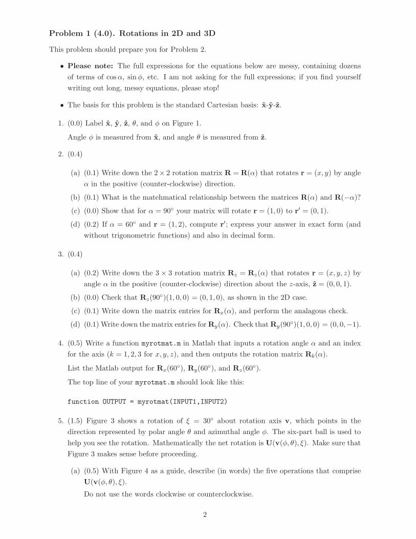
Problem 1 (4.0). Rotations in 2D and 3D

This problem should prepare you for Problem 2.

• Please note: The full expressions for the equations below are messy, containing dozens

of terms of cos α, sin φ, etc. I am not asking for the full expressions; if you find yourself

writing out long, messy equations, please stop!

• The basis for this problem is the standard Cartesian basis: x-y-z.

1. (0.0) Label x, y, z, θ, and φ on Figure 1.

Angle φ is measured from x, and angle θ is measured from z.

2. (0.4)

(a) (0.1) Write down the 2× 2 rotation matrix R = R(α) that rotates r = (x, y) by angle

α in the positive (counter-clockwise) direction.

(b) (0.1) What is the matehmatical relationship between the matrices R(α) and R(−α)?

(c) (0.0) Show that for α = 90◦ your matrix will rotate r = (1, 0) to r′ = (0, 1).

(d) (0.2) If α = 60◦ and r = (1, 2), compute r′; express your answer in exact form (and

without trigonometric functions) and also in decimal form.

3. (0.4)

(a) (0.2) Write down the 3 × 3 rotation matrix Rz = Rz(α) that rotates r = (x, y, z) by

angle α in the positive (counter-clockwise) direction about the z-axis, z = (0, 0, 1).

(b) (0.0) Check that Rz(90◦)(1, 0, 0) = (0, 1, 0), as shown in the 2D case.

(c) (0.1) Write down the matrix entries for Rx(α), and perform the analagous check.

(d) (0.1) Write down the matrix entries for Ry(α). Check that Ry(90◦)(1, 0, 0) = (0, 0,−1).

4. (0.5) Write a function myrotmat.m in Matlab that inputs a rotation angle α and an index

for the axis (k = 1, 2, 3 for x, y, z), and then outputs the rotation matrix Rk(α).

List the Matlab output for Rx(60◦), Ry(60

◦), and Rz(60◦).

The top line of your myrotmat.m should look like this:

function OUTPUT = myrotmat(INPUT1,INPUT2)

5. (1.5) Figure 3 shows a rotation of ξ = 30◦ about rotation axis v, which points in the

direction represented by polar angle θ and azimuthal angle φ. The six-part ball is used to

help you see the rotation. Mathematically the net rotation is U(v(φ, θ), ξ). Make sure that

Figure 3 makes sense before proceeding.

(a) (0.5) With Figure 4 as a guide, describe (in words) the five operations that comprise

U(v(φ, θ), ξ).

Do not use the words clockwise or counterclockwise.

2

(b) (1.0) Derive an expression for the matrix U(v(φ, θ), ξ) that rotates a vector r about

the (Cartesian) input vector v by angle ξ; this expression will be in terms of the matrix

functions Rx(α), Ry(α), Rz(α), where α is the rotation angle about the x-axis, y-axis,

or z-axis. (No numbers or terms like cos α should appear in your answer.)

6. (0.8) Write a new function myrotmat_gen.m that represents U(v, ξ); note that this function

will call your myrotmat.m function. WARNING: If you use the arctangent function, be sure

to use atan2(y,x), not atan(y/x).

(a) (0.2) Using myrotmat_gen.m, compute U(v, ξ) for input values of v = (2, 1, 2) and

ξ = 30◦. List U in decimal form.

(b) (0.1) Numerically check that U(−v,−ξ) gives the same result, and explain why this

is the case.

(c) (0.1) Numerically check that U(v, ξ)v = v, and explain why this is the case.

(d) (0.2) Numerically check that U is orthogonal and also a (right-handed) rotation matrix.

(e) (0.2) Apply the rotation to the point r0 = (2, 2, 1).

• List the rotated point r in decimal form.

• Check that the lengths of both vectors are equal (‖r‖ = ‖r0‖).• Check that the angle between v and r0 is the same as the angle between v and r.

In Problem 2, you will need to use an accurate version of myrotmat_gen.m. You can check

your function with the following output:

rotation axis is v = (2.000, 1.000, 2.000)

u = (0.667, 0.333, 0.667)

polar angle theta = 48.190 deg (0.841 rad)

azimuthal angle phi = 26.565 deg (0.464 rad)

R1 =

0.8944 0.4472 0

-0.4472 0.8944 0

0 0 1.0000

R2 =

0.6667 0 -0.7454

0 1.0000 0

0.7454 0 0.6667

R3 =

0.8660 -0.5000 0

0.5000 0.8660 0

0 0 1.0000

R4 =

0.6667 0 0.7454

0 1.0000 0

-0.7454 0 0.6667

R5 =

0.8944 -0.4472 0

0.4472 0.8944 0

3

0 0 1.0000

U =

0.9256 -0.3036 0.2262

0.3631 0.8809 -0.3036

-0.1071 0.3631 0.9256

If you get these results, then you did it! If not, then ask me for this function

to use in Problem 2. (But you will lose 1.0 point for this request.)

7. (0.4) Using the function globefun3.m, plot your rotation axis v, the initial point r0, and

the rotated point r, all within the same figure. Pencil in an arrow from r0 to r.

Note that globefun3.m inputs latitude (= 90 − θ) and longitude (= φ).

Problem 2 (4.0). From fault parameters to moment tensors, Part I

• Figure 5 shows the basics of the problem: given measurements of the angles strike, dip,

and slip, compute the 3 × 3 symmetric moment tensor. Study Figure 5 carefully before

proceeding.

• The calculation of the moment tensor requires a choice of a orthonormal basis for expressing

vectors and tensors; we will choose the Global Centroid Moment Tensor (GCMT) convention

of up-south-east, denoted as r-θ-φ.

You should not use any notation such as x, y, or z throughout this problem.

• You will utilize the function U(v, ξ) (myrotmat_gen.m) that you obtained in Problem 1.

(You should have checked that your function gets the results in Problem 1-5; otherwise get

a version of myrotmat_gen.m from me.)

• The dip is denoted by θ. (In Problem 1, θ was a generic polar angle.)

1. (0.5)

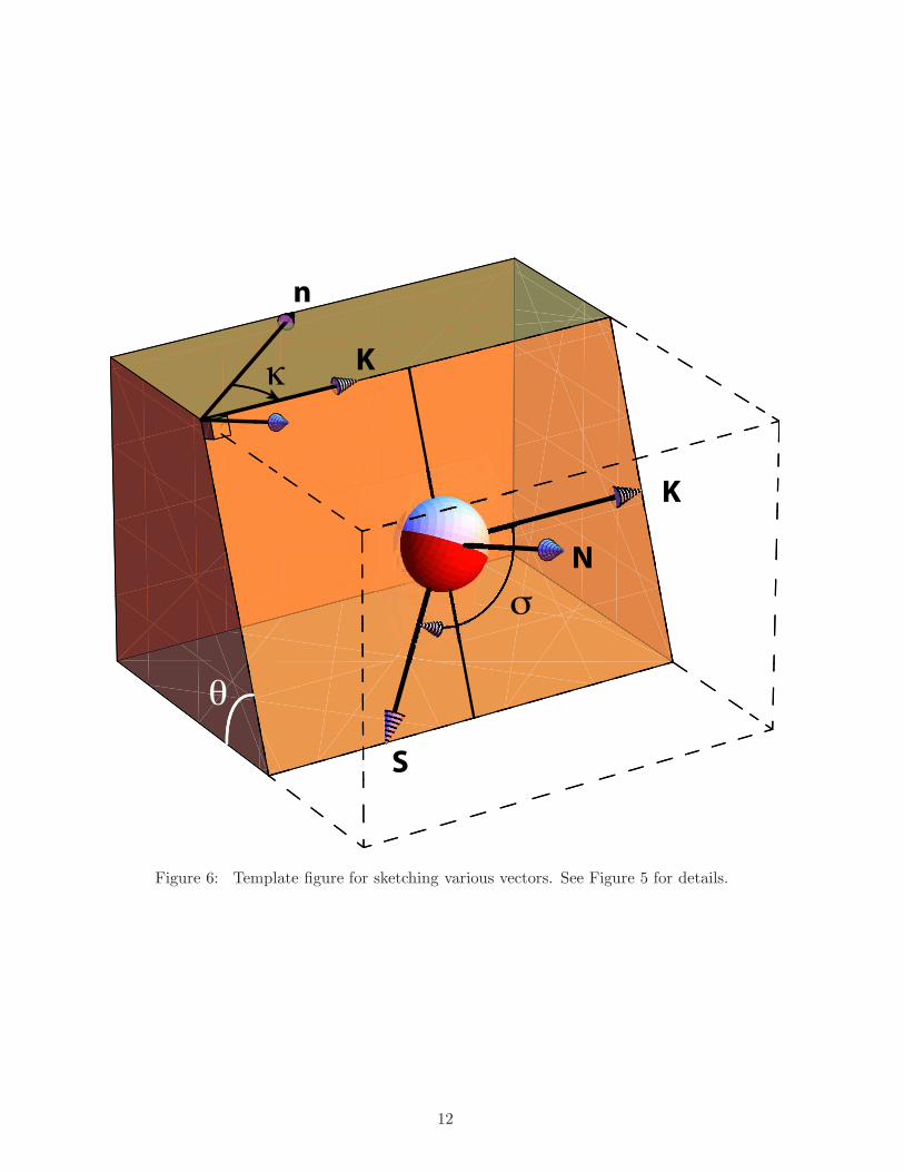
(a) (0.2) Sketch your basis vectors on Figure 6. “Your basis” is r (up), θ (south), φ (east).

(b) (0.3) The coordinates of the west vector are (0, 0,−1) in your basis.

What are the coordinates of the following vectors in your basis:

• the north vector n

• the zenith vector (“up”)

• the nadir vector (“down”)

2. (1.5) See Figure 5. In Problem 1, you used the expression

r = U(v, ξ)r0 (2)

Here you want to write similar abstract expressions for K, N, S. (What are v, ξ, and r0

for each case?) Please also describe each expression in words.

(a) the strike vector K

4

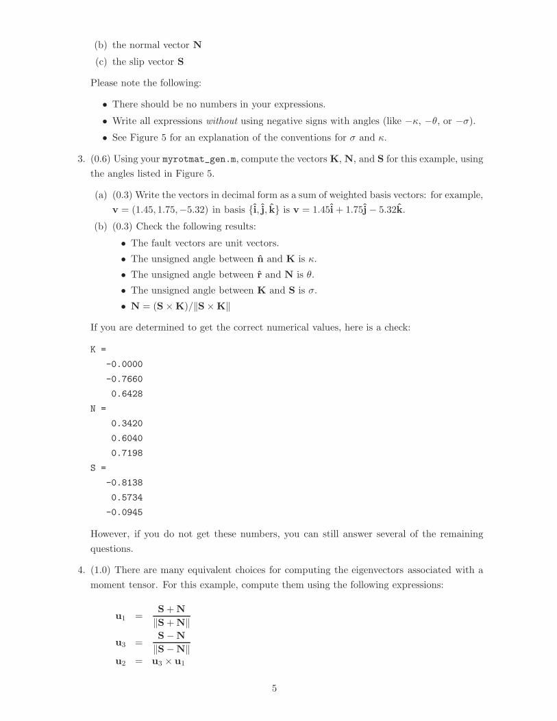
(b) the normal vector N

(c) the slip vector S

Please note the following:

• There should be no numbers in your expressions.

• Write all expressions without using negative signs with angles (like −κ, −θ, or −σ).

• See Figure 5 for an explanation of the conventions for σ and κ.

3. (0.6) Using your myrotmat_gen.m, compute the vectors K, N, and S for this example, using

the angles listed in Figure 5.

(a) (0.3) Write the vectors in decimal form as a sum of weighted basis vectors: for example,

v = (1.45, 1.75,−5.32) in basis {i, j, k} is v = 1.45i + 1.75j − 5.32k.

(b) (0.3) Check the following results:

• The fault vectors are unit vectors.

• The unsigned angle between n and K is κ.

• The unsigned angle between r and N is θ.

• The unsigned angle between K and S is σ.

• N = (S × K)/‖S × K‖

If you are determined to get the correct numerical values, here is a check:

K =

-0.0000

-0.7660

0.6428

N =

0.3420

0.6040

0.7198

S =

-0.8138

0.5734

-0.0945

However, if you do not get these numbers, you can still answer several of the remaining

questions.

4. (1.0) There are many equivalent choices for computing the eigenvectors associated with a

moment tensor. For this example, compute them using the following expressions:

u1 =S + N

‖S + N‖

u3 =S −N

‖S −N‖u2 = u3 × u1

5

The columns of U are u1, u2, and u3.

(a) (0.1) List U.

(b) (0.1) Check that U is an orthogonal matrix.

(c) (0.1) Compute the determinant to check that the basis is also a rotation matrix.

(d) (0.1) Check that u2 is in the fault plane and 90◦ from the slip vector.

(e) (0.6) Draw three points on the beachball in Figure 6 that correspond to where the

axes {u1,u2,u3} pierce the beachball. If needed, explain in words what directions the

axes point.

5. (0.0) What are the (unsorted) eigenvalues of any double-couple moment tensor?

6. (0.3) Our convention for (eigen)basis U is tied to eigenvalues ordered as λ1 = 1, λ2 = 0,

λ3 = −1. Thus, our “base” diagonal moment tensor is M′ with diagonal (1, 0,−1).

(a) Write the equation for M, obtained from M′ via transformation by U.

Hint: Think eigen-decomposition.

(b) List M in numerical form.

Problem 3 (2.0). From fault parameters to moment tensors, Part II

1. (0.6) From Problem 2, you obtained the moment tensor M for the fault in Figure 5.

(a) (0.2) Check that the following operations are true for this example:

Mu1 = λ1 u1 = u1 (3)

Mu2 = λ2 u2 = 0 (4)

Mu3 = λ3 u3 = −u3 (5)

MS = N (6)

MN = S (7)

(b) (0.4) What is the physical meaning of each of these operations? (Be careful: The

“beachball” pattern is representative of the P-wave motion only.)

2. (0.5) Compute the transformation matrix P that will convert the coordinates of vectors

and tensors from the up-south-east basis to the north-east-down basis of Aki and Richards

(2002).

(a) (0.2) Compute P using Eq. 1 of Section A.5.1 of Stein and Wysession (2003).

(b) (0.2) Transform the fault vectors K, N, S using K′ = PK, etc.

Sketch K′, N′, and S′ in Figure 6.

(c) (0.1) Transform M to M′ using M′ = PMPT ; list the values of moment matrix M ′.

3. (1.0) Go to www.globalcmt.org/CMTsearch.html and enter the following search parame-

ters:

6

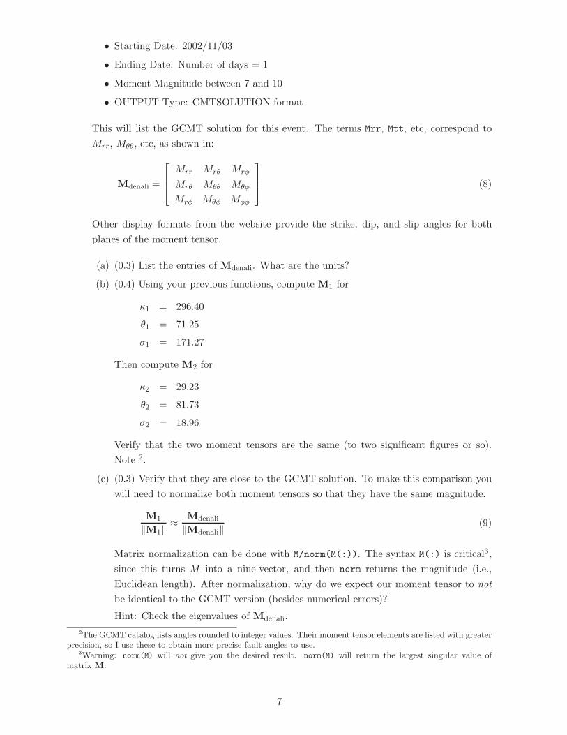
• Starting Date: 2002/11/03

• Ending Date: Number of days = 1

• Moment Magnitude between 7 and 10

• OUTPUT Type: CMTSOLUTION format

This will list the GCMT solution for this event. The terms Mrr, Mtt, etc, correspond to

Mrr, Mθθ, etc, as shown in:

Mdenali =

Mrr Mrθ Mrφ

Mrθ Mθθ Mθφ

Mrφ Mθφ Mφφ

(8)

Other display formats from the website provide the strike, dip, and slip angles for both

planes of the moment tensor.

(a) (0.3) List the entries of Mdenali. What are the units?

(b) (0.4) Using your previous functions, compute M1 for

κ1 = 296.40

θ1 = 71.25

σ1 = 171.27

Then compute M2 for

κ2 = 29.23

θ2 = 81.73

σ2 = 18.96

Verify that the two moment tensors are the same (to two significant figures or so).

Note 2.

(c) (0.3) Verify that they are close to the GCMT solution. To make this comparison you

will need to normalize both moment tensors so that they have the same magnitude.

M1

‖M1‖≈ Mdenali

‖Mdenali‖(9)

Matrix normalization can be done with M/norm(M(:)). The syntax M(:) is critical3,

since this turns M into a nine-vector, and then norm returns the magnitude (i.e.,

Euclidean length). After normalization, why do we expect our moment tensor to not

be identical to the GCMT version (besides numerical errors)?

Hint: Check the eigenvalues of Mdenali.

2The GCMT catalog lists angles rounded to integer values. Their moment tensor elements are listed with greaterprecision, so I use these to obtain more precise fault angles to use.

3Warning: norm(M) will not give you the desired result. norm(M) will return the largest singular value ofmatrix M.

7

Problem

Approximately how much time outside of class and lab time did you spend on this problem set?

Feel free to suggest improvements here.

References

Aki, K., and P. G. Richards (2002), Quantitative Seismology, 2 ed., University Science Books,

San Francisco, Calif., USA, 2009 corrected printing.

Shearer, P. M. (2009), Introduction to Seismology, 2 ed., Cambridge U. Press, Cambridge, UK.

Stein, S., and M. Wysession (2003), An Introduction to Seismology, Earthquakes, and Earth

Structure, Blackwell, Malden, Mass., USA.

−1

0

1−1 −0.5 0 0.5 1

−1

−0.8

−0.6

−0.4

−0.2

0

0.2

0.4

0.6

0.8

1

x

y

z

Figure 1: A point on the sphere: φ = 40◦ (azimuthal angle), θ = 30◦ (polar angle).

8

λ3

p1

p2

λ2

λ1

DC

CLVD

CLVD

ISO

p3

Figure 2: Eigenvalue space for moment tensors; the three axes correspond to the eigenvalues.The purple plane is the deviatoric plane λ1 + λ2 + λ3 = 0. The brown planes are the coordinateplanes λ1 = 0, λ2 = 0, and λ3 = 0. ISO is the (1, 1, 1) direction; DC is the (1,−1, 0) direction.The principal axes of the moment tensor are denoted by p1, p2, and p3. The space of doublecouples represents all solutions that are deviatoric (purple plane) and have one eigenvalue thatis zero (brown planes).

x

y

z

v

x

y

z

v

U

Figure 3: The basic idea of the rotation in Problem 1. Operation U(v, ξ) will take a point onthe beachball and rotate it by ξ about v. Here ξ = 30◦; to see this, note that the ∆φ incrementbetween longitude lines is 15◦; the ∆θ increment between latitude lines is 15◦.

9

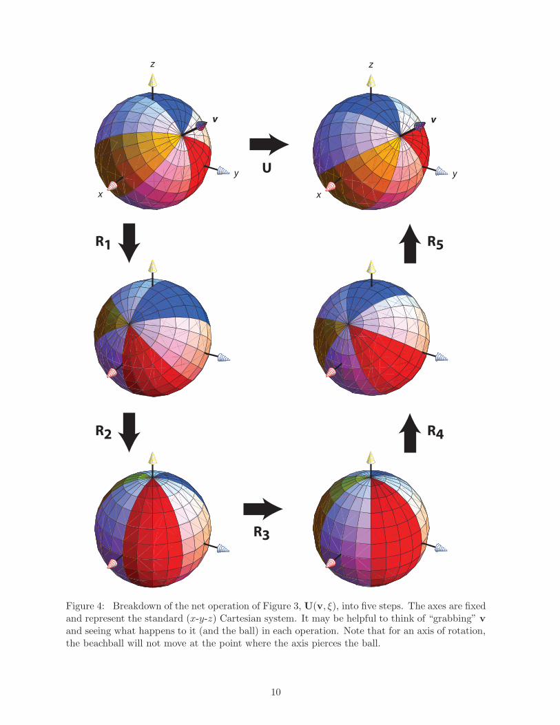
x

y

z

v

x

y

z

v

R1

R2

R3

U

R4

R5

Figure 4: Breakdown of the net operation of Figure 3, U(v, ξ), into five steps. The axes are fixedand represent the standard (x-y-z) Cartesian system. It may be helpful to think of “grabbing” vand seeing what happens to it (and the ball) in each operation. Note that for an axis of rotation,the beachball will not move at the point where the axis pierces the ball.

10

Map View Map View

K

K

n n

nn

K

K

KK

N

N N

NN

N N

S S

SS

K K

κ κ

κκ

θ θ

σ σ

κ = 40ο, θ = 70ο, σ = −120ο

Figure 5: Diagram showing notation for vectors and angles for Problem 2. n is the north vector,N is the fault normal vector, K is the strike vector, and S is the slip vector. The strike angleis κ = 40◦, the dip angle is θ = 70◦, and the slip angle is σ = −120◦. The slip angle is the(signed) angle between the strike vector and the slip vector. The sign of σ is determined fromthe direction of N: rotate K to S along the shortest angle; if that rotation is counterclockwise,with N determining “up,” then the angle is positive. (In other words, if K×S is in the directionof N, then σ > 0; otherwise σ < 0.) Another way of explaining it is that you rotate K to Sclockwise (looking down N); the resultant angle is between 0◦ and 360◦. By convention, the angleis “wrapped” to the interval [−180◦, 180◦], similar to the choice in longitude conventions. In thisexample σ = 240◦ = −120◦. Note that the fault vectors N and S always “sandwich” the coloredquadrant of the beachball, which contains T = u1 at its center. T is the T -axis, which is theeigenvector associated with positive eigenvalue, λ1. This can be remembered from the fact thatT = (N + S)/

√2.

11

n

K

K

N

S

κ

θ

σ

Figure 6: Template figure for sketching various vectors. See Figure 5 for details.

12