Problems in Physics wi th Many Scales of Length

Physical systems as varied as magnets and fluids are ahke J'n having

fluctuations in structure over a vast range of sizes. A novel method

called the renormahzation group has been invented to explain them

One of the more conspicuous prop­erties of nature is the great di­versity of size or length scales in

the str ucture of the world. An ocean, for example, has c urrents that persist for tho usands of kilometers and has tides of global extent; i t also has waves that range in s ize from less than a centimeter to several meters; at m uch finer resolu­tion seawater must be regarded as an aggregate of molec ules whose charac­teristic scale of length is roughly 1 0-8 centimeter. From the smallest structure to the largest is a span of some 1 7 or­ders of magnitude.

In general , events distinguished by a great d isparity in size have little influ­ence on one another; they do not com­m unicate, and so the phenomena asso­c iated with each scale can be treated independently. The interaction of two adjacent water molec ules is much the same whether the molecules are in the Pacific Ocean or in a teapot. What is eq ually important, an ocean wave can be described quite acc urately as a dis­turbance of a continuous fluid, ignoring ent irely the molec ular structure of the liquid . The success of almost all practi­cal theories in physics depends on isolat­ing some limited range of length scales. If it were necessary in the eq uations of hydrodynamics to spec ify the motion of every water molecule, a theory of ocean waves would be far beyond the means of 20th-cent ury science.

A class of phenomena does ex' ist, however, where events at many scales of length make contr ibutions of equal im­portance. An example is the behavior of water when it is heated to boil ing under a press ure of 2 1 7 atmospheres. At that pressure water does not boil until the temperat ure reaches 647 degrees Kel­vin. This combination of pressure and temperature defines the cr itical point of water, where the distinction between liq­uid and gas disappears; at higher pres­sures there is only a single, undifferenti­ated fluid phase, and water cannot be made to boil no matter how much the

158

by Kenneth G. Wilson

temperature is raised. Near the criti­cal point water develops fluctuations in density at all possible scales. The fluctu­ations take the form of drops of l iquid thoroughly interspersed with b u bbles of gas, and there are both drops and b u b­bles of all sizes from single molecules up to the volume of the specimen. Precisely at the critical point the scale of the larg­est fl uctuations becomes infinite, but the smaller fluctuations are in no way di­minished . Any theory that describes wa­ter near its critical point must take into account the entire spectrum of length scales.

M ul tiple scales of length complicate many of the outstanding problems in theoretical physics and in certain other fields of study. Exact solutions have been found for only a few of these prob­lems, and for some others even the best­known approximations are unsatisfac­tory. In the past decade a new method called the renormalization group has been introduced for dealing with prob­lems that have m ultiple scales of length . I t has by no means made the problems easy, but some that have resisted all oth­er approaches may yield to this one.

The renormalization group is not a descriptive theory of nature but a gener­al method for constr uct ing theories. It can be applied not only to a fluid at the critical point but also to a ferromagnetic material at the temperature where spon­taneous magnetization first sets in, or to a mixture of l iquids at the temperat ure where they become fully miscible, or to

an alloy at the temperat ure where two kinds of metal atoms take on an orderly d istr ibution. Other problems that have a su itable form include turbulent flow, the onset of superconductivity and of su­perfluid ity, the conformation of poly­mers and the binding together of the e le ­mentary particles called quarks. A re ­markable hypothesis that seems to be confirmed by work with the renormali­zation group is that some of these phe­nomena, which superficially seem quite distinct, are identical at a deeper lev­el. For example, the critical behavior of fluids, ferromagnets, liquid mixtures and alloys can all be described by a sin­gle theory.

The most convenient context in which to discuss the operation of the renor­

malization group is a ferromagnet, or permanent magnet. Ferromagnetic ma­terials have a critical point called the C urie point or the Curie temperature, after P ierre Curie, who studied the ther­modynamics of ferromagnets at about the turn of the century. For iron the Curie temperat ure is \,044 degrees K. At higher temperatures iron has no spontaneous magnetization. As the iron is cooled the magnetization remains zero until the Curie temperature is reached, and then the material abruptly becomes magnetized. If the temperature is reduced further, the strength of the magnetization increases smoothly .

Several properties of ferromagnets besides the magnet izat ion behave oddly

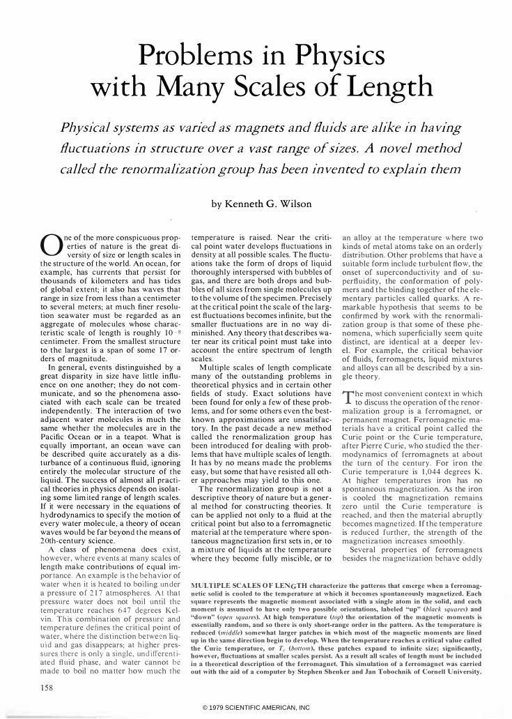
MULTIPLE SCALES OF LENGTH characterize the patterns that emerge when a ferromag­netic solid is cooled to the temperature at which it becomes spontaneously magnetized. Each square represents the magnetic moment associated with a single atom in the solid, and each moment is assumed to have only two possible orientations, labeled "up" (black sqllares) and "down" (opell sqllares). At high temperature (top) the orientation of the magnetic moments is essentially random, and so there is only short-range order in the pattern. As the temperature is reduced (middle) somewhat larger patches in which most of the magnetic moments are lined np in the same direction begin to develop. When the temperature reaches a critical value called the Curie temperature, or Tc (bottom), these patches expand to infinite size; significantly, however, fluctuations at smaller scales persist. As a result all scales of length must be included in a theoretical description of the ferromagnet. This simulation of a ferromagnet was carried out with the aid of a computer by Stephen Shenker and Jan Toboch.nik of Cornell University.

© 1979 SCIENTIFIC AMERICAN, INC

159

© 1979 SCIENTIFIC AMERICAN, INC

near the C ur ie point. Another property of interest is the magnetic susceptibility, or the change in magnetization induced by a small applied field. Well above the C urie point the susceptibility is small beca use the iron cannot retain any mag­netization; well below the C urie temper­ature the susceptibility is small again be­ca use the material is already magnetized and a weak applied field cannot change the state of the system very much. At temperatures close to 1 ,044 degrees, however, the susceptibil ity rises to a sharp peak, and at the C urie point itself the susceptibility becomes infinite.

The ultimate source of ferromagnet­ism is the quantum-mechanical spinning of electrons. Because each electron ro­tates it has a small magnetic dipole mo­ment; in other words, it acts as a magnet with one north pole and one south pole. How the spin of the e lectron gives rise to the magnetic moment will not concern me here. It is sufficient to note that both the spin and the magnetic moment can be represented by a vector, or arrow,

t " f\

M = +4 M = +2 ]'IP = .273" P = .037

1 "

which defines the direction of the elec­tron's magnetic field.

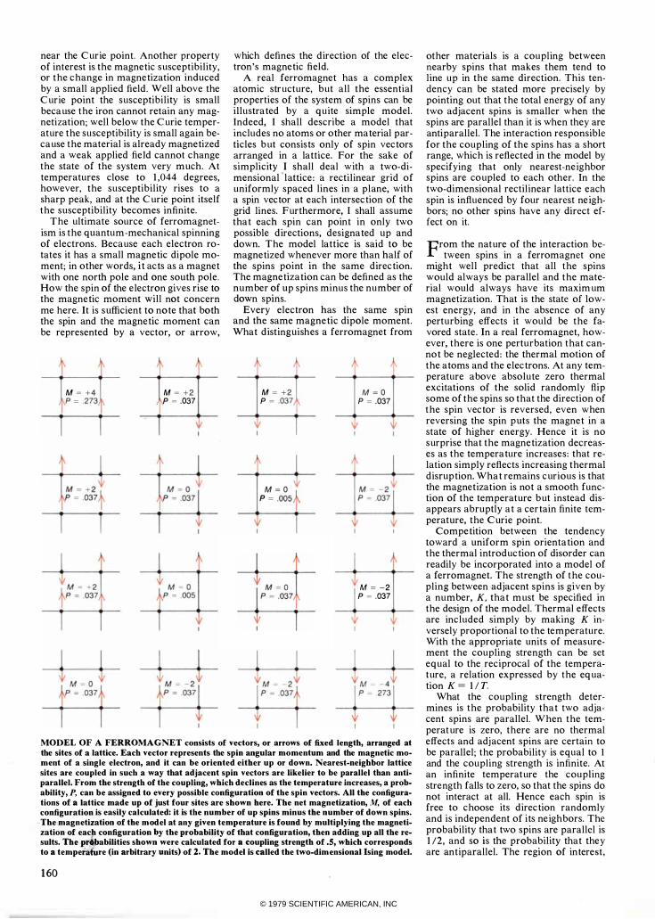
A real ferromagnet has a complex atomic str ucture, but all the essential properties of the system of spins can be il lustrated by a quite simple model. Indeed, I shall describe a model that includes no atoms or other material par­ticles b ut consists only of spin vectors arranged in a lattice. For the sake of simplicity I shall deal with a two-di­mensional'lattice : a recti linear grid of uniformly spaced lines in a plane, with a spin vector at each intersection of the grid lines. Furthermore, I shall assume that each spin can point in only two possible directions, designated up and down. The model lattice is said to be magnetized whenever more than half of the spins point in the same direction. The magnetization can be defined as the number of up spins minus the number of down spins.

Every electron has the same spin and the same magnetic dipole moment. What d ist inguishes a ferromagnet from

I f\

M = +2 P = .037"

M =0 P = .005+

B +4-

f\

"

M =0 P = .037

M =-2 P = .037

LJ MODEL OF A FERROMAGNET consists of vectors, or arrows of fixed length, arranged at the sites of a lattice. Each vector represents the spin angular momentum and the magnetic mo­ment of a single electron, and it can be oriented either up or down. Nearest-neighbor lattice sites are coupled in such a way that adjacent spin vectors are likelier to be parallel than anti­parallel. From the strength of the coupling, which declines as the temperature increases, a prob­ability, P, can be assigned to every possible configuration of the spin vectors. All the configura­tions of a lattice made up of just four sites are shown here. The net magnetization, M, of each configuration is easily calculated: it is the number of up spins minus the number of down spins.

··The magnetization of the model at any given temperature is found by multiplying the magneti-zation of. each configuration by the probability of that configuration, then adding up all the re­sults. The p!'�J1abilities shown were calculated for a coupling strength of .5, which corresponds to a temperature (in arbitrary units) of 2. The model is called the two-dim ensional Ising model.

160

other materials is a coupling between nearby spins that makes them tend to l ine up in the same direction. This ten­dency can be stated more precisely by pointing out that the total energy of any two adjacent spins is smaller when the spins are parallel than it is when they are anti parallel. The interaction responsible for the coupling of the spins has a short range, which is reflected in the model by specifying that only nearest-ne ighbor spins are co upled to each other. In the two-dimensional rectil inear lattice each spin is influenced by four nearest ne igh­bors; no other spins have any direct ef­fect on it.

From the nature of the interaction be­tween spins in a ferromagnet one

might well predict that all the spins would always be parallel and the mate­rial would always have its maxim um magnetization. That is the state of low­est energy, and in the absence of any perturbing effects it would be the fa­vored state . In a real ferromagnet, how­ever, there is one perturbation that can­not be neglected: the thermal motion of the atoms and the electrons. At any tem­perature above absolute zero thermal excitations of the solid randomly flip some of the spins so that the direction of the spin vector is reversed, even when reversing the spin puts the magnet in a state of higher energy. Hence it is no surprise that the magnetization decreas­es as the temperature increases: that re­lation simply reflects increasing thermal disruption. What remains c urious is that the magnetization is not a smooth func­tion of the temperature b ut instead dis­appears abruptly at a certain finite tem­perature, the Curie point.

Competition between the tendency toward a uniform spin orientation and the thermal introduction of disorder can readily be incorporated into a model of a ferromagnet. The strength of the cou­pling between·adjacent spins is given by a number, K. that m ust be specified in the design of the model. Thermal effects are included simply by making K in­versely proportional to the temperature. With the appropriate units of measure­ment the coupling strength can be set equal to the reciprocal of the tempera­t ure, a relation expressed by the eq ua­tion K = 1 IT.

What the coupling strength deter­mines is the probability that two adja­cent spins are parallel. When the tem­perat ure is zero, there are no thermal effects and adjacent spins are certain to be parallel; the probability is equal to I and the coupling strength is infinite. At an infinite temperat ure the coupling strength falls to zero, so that the spins do not interact at all. Hence each spin is free to choose its d irection randomly and is independent of its ne ighbors. The probability that two spins are parallel is 1 /2, and so is the probability that they are anti parallel. The region of interest,

© 1979 SCIENTIFIC AMERICAN, INC

of co urse, lies between these extremes of temperature, where the probabil ity of the adjacent spins' lining up m ust always have a val ue between 1!2 and 1 .

Suppose there is a large two-dimen­sional lattice of spins and that some

one spin in it is artificially held fixed in the up orientation. What is the effect on the other spins? The effect on the spins at the four adjacent lattice sites is easy to imagine: since they are d irectly coupled to the fixed spin, they will have a greater-than-even probability of point­ing up. The extent to which the probabil­ity is biased depends on the value of K, which is determined in turn by the tem­perature.

More d istant spins have no direct in­teraction with the fixed spin, but none­theless the infl uence of the fixed spin does not end with the immediate neigh­bors. Because the nearest-neighbor spins tend to point up more often than down they create a similar bias in their own nearest neighbors. In this way the d is­t urbance can propagate over a large area of the lattice. The range of influ­ence of a single fixed spin can be mea­sured by observing the orientation of many spins that are all at the same large d istance from the fixed one. If re­versing the orientation of the fixed spin from up to down increases the number of down spins in the d istant population, then the spins are said to be correlated. The maximum d istance over which such a correlation can be detected is called the correlation length. Regions separat­ed by a distance greater than the correla­tion length are essentially independent.

In a lattice at very high temperature the correlation length is close to zero. The distribution of spins is nearly ran­dom, and so the average number of up and down spins must be equal; in other words, the magnetization is zero. As the temperature falls (and the coupling strength increases) correlations over larger d istances begin to appear . They take the form of spin fluctuations, or patches of a few spins each that mostly point in the same d irection. Over any large area the magnetization is still zero, but the structure of the lattice is m uch d ifferent from what it was near infinite temperature.

As the temperature approaches the C urie point the correlation length grows rapidly. The basic interactions of the model have not changed; they still con­nect only adjacent lattice sites, but long­range order has emerged from the short­range forces. What is most significant in the growth of the correlation length is that as the maxim um size of the spin fluctuations increases, the smaller fl uc­tuations are not suppressed; they merely become a finer structure superimposed on the larger one. The largest fluctua­tions are not areas of uniform spin align­ment; they include many smaller fl uctu­ations and can be d istinguished only be-

z o � N i= w z CJ

I I I I I I I 1 l� I::J � Ia: l� I� I� IiI IG 1

>­I­:::::; CD ti: w o (fJ ::J (fJ

:Ii TEMPERATURE -7 (fJ O l-----------"------f---------------! 0 ::J o w Z � Z o 0.. (fJ

z 3: o a

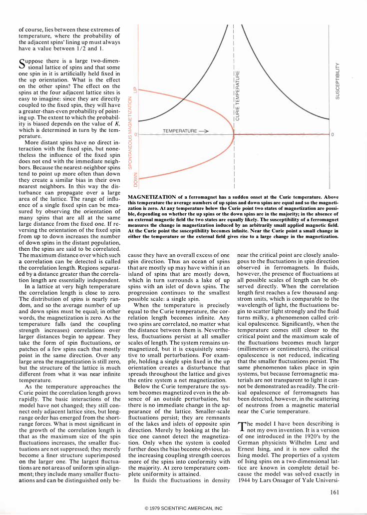
MAGNETIZATION of a ferromagnet has a sudden onset at the Curie temperature. Above this temperature the average numbers of up spins and down spins are equal and so the magn eti­zation is zero. At any temperature below the Curie point two states of magnetization are possi­ble, depending on whether the up spins or the down spins are in the majority; in the absence of an external magnetic field the two states are equally likely. The susceptibility of a ferromagn et measures the change in magnetization induced by an arbitrarily small applied magnetic field. At the Curie point the susceptibility becom es infinite. Near the Curie point a small change in either the temperature or tbe external field gives rise to a large change in the magn etization.

cause they have an overall excess of one spin d irection. Thus an ocean of spins that are mostly up may have within it an island of spins that are mostly down, which in turn s urrounds a lake of up spins with an islet of down spins. The progression continues to the smallest possible scale : a single spin.

When the temperature is precisely equal to the C urie temperature, the cor­relation length becomes infinite. Any two spins are correlated, no matter what the d istance between them is. Neverthe­less, fl uctuations persist at all smaller scales of length. The system remains un­magnetized, but it is exquisitely sensi­tive to small perturbations. For exam­ple, holding a single spin fixed in the up orientation creates a disturbance that spreads throughout the lattice and gives the entire system a net magnetization.

Below the C urie temperature the sys­tem becomes magnetized even in the ab­sence of an outside perturbation, but there is no immediate change in the ap­pearance of the lattice. Smaller-scale fl uctuations persist; they are remnants of the lakes and islets of opposite spin d irection. Merely by looking at the lat­tice one cannot detect the magnetiza­tion. Only when the system is cooled further does the bias become obvious, as the increasing coupling strength coerces more of the spins into conformity with tpe majority. At zero temperature com­plete uniformity is attained .

In fluids the fluctuations in density

near the critical point are closely analo­gous to the fluctuations in spin d irection observed in ferromagnets. In fl uids, however, the presence of fluctuations at all possible scales of length can be ob­served directly. When the correlation length first reaches a few thousand ang­strom units, which is comparable to the wavelength of light, the fluctuations be­gin to scatter l ight strongly and the fl uid turns milky, a phenomenon called crit­ical opalescence. Significantly, when the temperature comes still closer to the critical point and the maximum scale of the fluctuations becomes m uch larger (millimeters or centimeters), the critical opalescence is not reduced, indicating that the smaller fluctuations persist. The same phenomenon takes place in spin systems, but because ferromagnetic ma­terials are not transparent to l ight it can­not be demonstrated as readily. The crit­ical opalescence of ferromagnets has been detected, however, in the scattering of neutrons from a magnetic material near the C urie temperature .

The model I have been describing is not my own invention. It is a version

of one introduced in the 1920's by the German physicists Wilhelm Lenz and Ernest Ising, and it is now called the Ising model. The properties of a system of Ising spins on a two-dimensional lat­tice are known in complete detail be­cause the model was solved exactly in 1944 by Lars Onsager of Yale Universi-

161

© 1979 SCIENTIFIC AMERICAN, INC

As your introduction to

The Library of Science Choose either

this $67.50 Classic for only $3.95 A saving of 94% Edited by' Douglas M. Considine. Nearly 200 experts have contributed to this thoroughly revised and greatly expanded fifth edition of the most authoritative single-volume source of scientific knowledge ever assembled. Enormous 91f4" x 12" volume contains 2.2 million words, 2382 pages, 2500 photographs, drawings and charts, and 500 tables. 7200 articles cover mathematics, from information sciences to physics and chemistry . .. . . . an amazing book ... for both the general and scientific reader. " -The New York Times

any other 3 books for only $3.95 if you will join now for a trial period and agree to take 3 more books-at handsome d iscounts-over the next 12 months.

(values to $75.00) (Publishers' Prices shown)

162

54995. THE ILLUS­

T RATED ENCY­

CLOPEDIA OF .\R·

CH AEOLOG Y. Glyn Daniel. $17.95

44905. THE ENCY­CLOPEDIA OF HOW IT'S MADE. $14.95

55000. T HE ILLUS·

T RATED ENCY·

C L O P EDIA O F

ASTRONOMY A ND

SPACE. $16.95

74300-2. ROME AND HER EMPIRE. Barry

Cunliffe. A magnifi­cently illustrated volume t h a t m ake s t h e history of one of the world's greatest civiliza­t i o n s c o m e a l i v e . Counts as 2 of your 3 books. $50.00

communication and con� with .

.. Extraterrestrial Life , 'an RJdpaIh .. .�' it..

..., ... :"I'

74771. MES SA GES FROM THE STA RS!

T HE RUNAWA Y

UNIVERSE. A report on the efforts of scien­tists to locate traces of interstellar communica­tion. Plus. the gripping and dramatic story of the birth and death of the cosmos from the Big Bang to titanic future holocaust. The 2 coulll as one book. $19.95

63340-2. MYSTERIES OF THE PAST . Cap­tivating investigation of prehistory and great rid­dles. Outsized. Sumptu­ously illustrated. COli/liS as 2 of your 3 books.

$34.95

© 1979 SCIENTIFIC AMERICAN, INC

3 47 40. ATLAS O F MAN . C o v e r s 400 gro u p s of p eo p l e s , tribes, and nations. 120 color photographs, 350 maps and line illus­trations. Covers geog­raphy, land use, culture, climate, religion, much more. $2 5.00

4 65 80 ·2 . T H E EVOLVING CONTI· N ENTS . Br i a n F. Windley. An integrated global overview of the geosciences. Counts as 2 of y o u r 3 b o o k s .

$34.95

8057 0. ST E L LAR A T M OSPHER ES . Dimitri Mihalas. An au­thoritative report on the stellar envelope, modes of energy transport in this atmosphere, rates of star mass loss, and much

$24.95

4883 0: FRACTALS, FORM , C HAN C E

AND DIMENSION . Benoit B. Mandelbrot. A brilliant geometrical investigation into the fragmented and irregular pat t e rn s of na­ture. $17.50

422 85. DIRECTIONS r i IN PHYSICS. Pau l , A.M. Dirac. One of the ! gre a te s t t h eore tical I ii physicists of the twen- i ! tieth century presents his :,',1" views on cosmological t h eo r i e s , q u a n t u m ,1 t h e o r y , q u a n t u m mechanics and quantum electrodynamics.

$1 2.95

662 75-2 . THE ORI­GIN OF THE SOLAR SYSTEM. Edited by S. F. Dermott. A compila­tion of the views of 28 leading astronomers, as­trbp h y s i c i s t s , c o s ­mologists and mathema­ticians covering theories of stellar formation. Counts as 2 of your 3 books. $39.00

Tt4E ANIU.YSIS OF INFOffMATION SYSTEMS ;""..\----

,'_" .,', "'.," ,w¥

� ........... ",." ,

81403. SUN, MOON, AND STAN D I N G STONES. John Edw in Wood. I ncludes the latest findings from resear­chers in archaeology, as­tronomy, climatology, a n d p h ys i c s. il l u s­trated. $14.95

39746·2 . CO MPAN· ION TO CONCRETE MA THE MATI C S . Volumes I and II. Z. A.

Me/zak. Mathematical techniques and various applications. The set counts as 2 of your 3 books. $46.45

41 610 . DA T A AN AL YSIS F O R S C I ENTISTS AND ENGINEERS. Stuart L. Meyer. 513-page vol­ume covers all the statis­tical methods, concepts, and analysis techniques that any experimenter will probably ever need.

$19.95

40167·2. THE CON· D ENSED CHEMI· CAL DICTIONARY. Updated to meet today's n eeds. Over 18,000 entries. Counts as 2 of

your 3 books . $32.50

33430. THE ANALY· SIS OF INFORMA· TION SYSTEMS. Re· vised Edition. Charles T. Meadow . A distin­guished computer au­thority offers an all­inclusive treatment.

$20.95

3 7 34 7 . CASTE AND ECOL OGY IN THE SOCIAL INSECTS. Oster and Wilson.

$20.00

34 210. T HE AR· CHAEOLOGY OF NOKfH AME RICA. Dean Snow. Prehistoric Indian cultures, from the first crossings into t his continent to t h e 20t h c e n t u r y. 195 photo s , c h a r t s a n d maps. $18.95

7 3940. THE REST· LESS UNI VERSE . Henry L. S hipman. A highly acclaimed 450-page tour of the ideas, principles, and process of modern astronomy.

$16.95

3 8362·2. CLIMATIC CHANGE. Dr. Joh n

Gribbin. Provides a n A to Z report on the basic pieces and patterns of t h e e a r t h's r i c h climatological puzzle. Counts as 2 of your 3 books. $32.50

74590. THE ROOTS O F CIVILIZATION. Alexander Marshack. A remarkable re-creation of the life of prehistoric man. Illustrated. $1 7.50

87610. THE WORLD ENERG Y BOOK. Crabbe and McBride. O ver 1500 alphabeti­cally arranged entries on everything from fossil fuels to power from sewage. Includes 35 wor l d m a p s a n d 40 pages of t ables, dia· grams, and charts.

If the reply card has been removed, please write to The Library of Science Dept. 2 -B6A, Riverside, N.J. 08370

$25.00

to obtain membership information and application.

163

© 1979 SCIENTIFIC AMERICAN, INC

ty. Since then sol utions have also been found for several other two-dimension­al models (whereas no three-dimension­al model has yet been solved exactly) . Nevertheless, the problems of describ­ing two-d imensional systems are far from trivial. In what follows I shall apply the methods of the renormaliza­tion group to the two-dimensional Is ing model as if it were a problem still out­standing, and Onsager's sol ution will serve as a check on the results.

What does it mean to solve or to un­derstand a model of a physical system? In the case of the Ising system the micro­scopic properties are known completely from the outset, since they were speci­fied in building the model. What is need­ed is a means of predicting the macro­scopic properties of the system from the known microscopic ones. For example, a formula giving the spontaneous mag­netization, the susceptibil ity and the correlation length of the model as a function of temperature would contrib­ute greatly to understanding.

It is not notably difficult to calc ulate the macroscopic properties of any given config uration of the spins in an Ising model. The magnetization, for example, can be determined simply by counting the number of up spins and the n umber of down spins and then subtracting. No one config uration of the spins, however,

1 X 1030

2 x 102•

2 X 10'. (fl z 0 � 6 X 10" a: � (') u:: 7 X 10'0 z 0 0 z 0:: 3 X 10' (fl LL 0 a: 65,536 w aJ ::;: � z

512

16

2 I

determines the macroscopic properties of the system. Instead all possible con­fig urations contribute to the observed properties, each in proportion to its prob­ability at a given temperat ure.

In principle the macroscopic proper­ties could be calculated directly as the sum of all the separate contributions. First the magnetization would be found for each configuration and then the cor­responding probability. The actual mag­netization would be obtained by m ulti­plying each of these pairs of numbers and adding up all the results. The sus­ceptibility and the correlation length could be found by proced ures that are not much more elaborate. The common element in all these calc ulations is the need to determine the probabilities of all possible config urations of the spins. Once the d istr ibution of probabilities is known the macroscopic properties fol­low directly,

As I pointed out above, the probabili­ty of any two adjacent spins' being par­allel is determined solely by the cou­pling strength K, which I have defined as the reciprocal of the temperature. If the probability of two neighboring spins in isolation being parallel is denoted p, then the probability of their being anti­parallel must be 1 - p. From these two values alone the relative probability of any spec ified configuration of a lattice

1 x 1 2 x 2 3 x 3 4 x 4 5 x 5 6 x 6 7 x 7 8 x 8 9 x 9 10 x 10 LATTICE S IZE

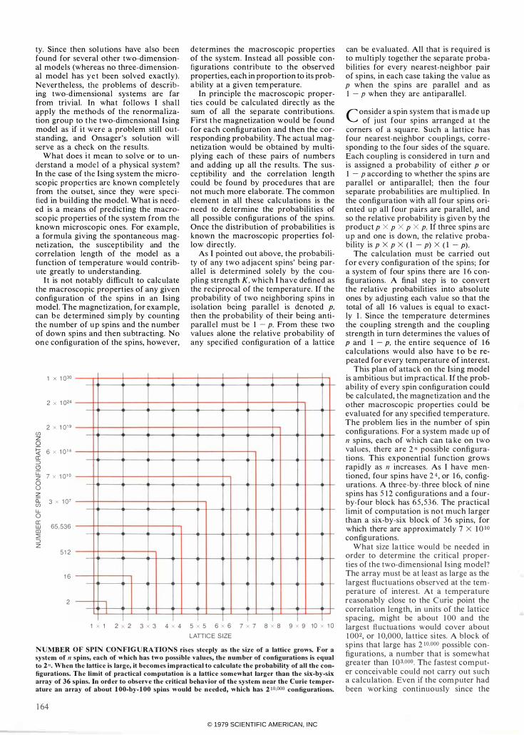
NUMBER OF SPIN CONFIGURATIONS rises steeply as the size of a lattice grows. For a system of II spins, each of which has two possible values, the number of configurations is equal to 2n. When the lattice is large, it becomes impractical to calculate the probability of all the con­figurations. The limit of practical computation is a lattice somewhat larger than the six-by-six array of 36 spins. In order to observe the critical behavior of the system near the Curie temper­ature an array of about lOO-by-lOO spins would be needed, which has 210,000 configurations.

164

can be evaluated. All that is required is to multiply together the separate proba­bilities for every nearest-neighbor pair of spins, in each case taking the value as p when the spins are parallel and as I - p when they are anti parallel .

Consider a spin system that is made up of j ust four spins arranged at the

corners of a square. Such a lattice has four nearest-neighbor couplings, corre­sponding to the four sides of the square. Each coupling is considered in t urn and is assigned a probability of e ither p or I - p accord ing to whether the spins are parallel or antiparallel; then the four separate probabilities are m ultiplied. In the config uration with all fo ur spins ori­ented up all four pairs are parallel, and so the relative probability is given by the prod uct p X P X P X p. If three spins are up and one is down, the relative proba­bility is p X p X ( I - p) X (1 - pl.

The calculation must be carried out for every configuration of the spins; for a system of four spins there are 1 6 con­fig urations. A final step is to convert the relative probabilities into absol ute ones by adj usting each value so that the total of all 1 6 val ues is eq ual to exact­ly 1 . Since the temperature determines the coupling strength and the coupling strength in turn determines the values of p and 1 - p, the entire seq uence of 1 6 calculations would also have t o b e re­peated for every temperature of interest.

This plan of attack on the Ising model is ambitious but impractical. If the prob­ability of every spin config uration could be calculated, the magnetization and the other macroscopic properties could be eval uated for any specified temperature. The problem lies in the number of spin config urations. For a system made up of 11 spins, each of which can take on two values, there are 2n possible configura­tions. This exponential function grows rapidly as 11 increases. As I have men­tioned, fo ur spins have 24, or 1 6, config­urations. A three-by-three block of nine spins has 512 configurations and a four­by-four block has 6 5 , 5 36. The practical limit of computation is not much larger than a six-by-six block of 36 spins, for which there are approximately 7 X 1 0 to con fig ura tions.

What size lattice would be needed in order to determine the critical proper­ties of the two-dimensional Is ing model? The array must be at least as large as the largest fluct uations observed at the tem­perat ure of interest. At a temperature reasonably close to the C urie point the correlation length, in units of the lattice spacing, might be about 1 00 and the largest fl uctuations would cover about 1002, or 10,000, lattice sites. A block of spins that large has 2 10,000 possible con­figurations, a number that is somewhat greater than 1 03,00°. The fastest comput­er conceivable could not carry out s uch a calcu lation. Even if the computer had been working continuo usly since the

© 1979 SCIENTIFIC AMERICAN, INC

"big bang" with which the universe be­gan, it would not yet have made a signifi­cant start on the task.

The need to carry out an almost end­less enumeration of spin configurations can be circumvented for two special conditions of the lattice . When the tem­perature of the system is zero (so that the coupling strength is infinite), all but two of the configurations can be neglect­ed. At zero temperature the probability that a pair of spins will be anti parallel falls to zero, and therefore so does the probability of any configuration that in­cludes even one antiparallel pair. The only configurations that do not have at least one anti parallel pair are those in which all the spins are up or all are down. The lattice is certain to assume one of these configurations, and all oth­er configurations have zero probability.

At infinite temperature, where the coupling strength is zero, the probability d istribution is also much simplified. Ev­ery spin is then independent of its neigh­bors and its d irection at any instant can be chosen at random. The result is that every configuration of the lattice has equal probability.

Through these two shortcuts to the determination of the probability distri­bution it is a trivial exercise to calculate exactly the properties of the Ising model at absolute zero and at infinite tempera­ture. Acceptable methods of approxi­mation are also available for any tem­perature low enough to be considered close to zero or high eno ugh to be con­sidered close to infinity. The trouble­some region is between these extremes; it corresponds to the region of the crit­ical point. Until recently there was no practical and direct method of calculat­ing the properties of a system arbitrarily close to the critical point. The renormal­ization group provides such a method.

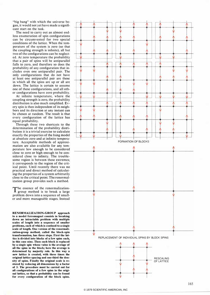
The essence of the renormalization­group method is to break a large

problem down into a sequence of small­er and more manageable stages. Instead

RENORMALIZATION-GROUP approach to a model ferromagnet consists in breaking down an intractable problem with multiple scales of length into a sequence of smaller problems, each of wbicb is confined to a single scale of length. One version of the renormali­zation-group method, called the block-spin transformation, has three steps. First the lat­tice is divided into blocks of a few spins each, in this case nine. Then each block is replaced by a single spin whose value is the average of all the spins in the block; here the average is determined by majority rule. In this way a new lattice is created, with three tim es the original lattice spacing and one-third the den­sity of spins. Finally the original scale is re­stored by reducing all dim ensions by a factor of 3. The procedure must be carried out for all configurations of a few spins in the origi­nal lattice, so that a probability can be found for every configuration of the block spins.

�

� II

I' II

V

V

II I'

\

I

\

\

I'

I'

I' \

I' I

f11' I'

FORMATION OF BLOCKS

I'

REPLACEME NT OF I NDIVIDUAL S P I N S ey BLOCK S P I N S

I'

II

RESCALING OF LATTICE

II

I I'

V

I'

I'

165 © 1979 SCIENTIFIC AMERICAN, INC

P ROBABILITIES OF NEAREST-N EIGHBOR CON FIG U RATIONS IN O RIGINAL LATTICE

Lj ------1' L- r-1 � � P = .3655 P = .1345 P = .1345 P = .3655

P ROBABILITIES OF SIX-SPIN CON FIG U RATIONS IN ORIGINAL LATTICE

WA P = .2943 � P = .0147 • P = .0020 � P = .0007

� P = .0398 � P = .0054 • P = .0002 � P = .0020 1--'\

VA P = .0147 � P = .0020 � P = .0007 � P = .0054

¥ :� __ .l. � P = .0054 � P = .0147 � P = .0020 � P = .0398

� P = .0054 � P = .0020 � P = .0054 ViA P = .0020

I P = .0007 � P = .0007 VA· P = .0007 � P = .0007

P = .0020

� P = .0020 VA P = .0020 � P = .0020

� P = .0007 P = .0147

� P = .0007

I P = .0147

- P = .0147 � P = .0007 P = .0147 P = .0007

- P = .0020 � P = .0020 - P = .0020

� P = .0020

� P = .0007 • P = .0007 � P = .0007 P = .0007

\1& P = .0020

;: P = .0054 V4 P = .0020

� P = .0054

� P = .0398 P = .0020 � P = .0147 P = .0054

� P = .0054 V4 P = .0007 � P = .0020

= P = .0147

V4 P = .0020

V4 P = .0002 VA P = .0054 P = .0398

'� P = .0007

V4 P = .0020 � P = .0147 � P = .2943

'\\1 -: --;If t t t t � � � t P = .4302 P = .0697 P = .0697 P = .4302

P ROBABILITIES OF N EAREST-NEIGHBOR BLOCK -SPIN CON FIGURATIONS

166

© 1979 SCIENTIFIC AMERICAN, INC

of keeping track of all the spins in a re­gion the size of the correlation length, the long-range properties are ded uced from the behavior of a few q uantities that incorporate the effects of many spins. There are several ways to do this. I shall describe one, the block-spin tech­nique, in which the principles of the method are revealed with particular clarity. It was introduced by Leo P. Kadanoff of the University of Chicago and was made a practical tool for cal­culations by Th. N iemeijer and J . M. J. van Lee uwen of the Delft University of Technology in the Netherlands.

The method has three basic steps, each of which must be repeated many times. First the lattice is divided into blocks of a few spins each; I shall em­ploy square blocks with three spins on a side, so that each block includes nine spins. Next all the spins in the block are averaged in some way and the entire block is replaced by a single new spin with the value of the average. Here the averaging can be done by a simple pro­ced ure: by following the principle of majority rule. If five or more of the orig­inal spins are up, the new spin is also up; otherwise it is down.

The result of these two operations is to create a new lattice whose fundamen­tal spacing is three times as large as that of the old lattice. In the third step the original scale is restored by reducing all dimensions by a factor of 3 .

These three steps define a renormali­zation-group transformation. Its effect is to eliminate from the system all fluc­tuations in spin d irection whose scale is smaller than the block size. In the model given here any fluctuation of the spins over a range of fewer than three lattice units will be smeared out by the averag­ing of the spins in each block. It is as if one looked at the lattice through an out­of-foc us lens, so that the smaller fea­t ures are blurred but the larger ones are unaffected.

It is not enough to carry out this pro­ced ure for any one configuration of the original lattice; once again what is sought is a probability distribution. S up­pose one considers only a small region of the initial lattice, consisting of 36 spins that can be arranged in four blocks. The spins in this region have 236,

or about 70 billion, possible configura­tions. After the block-spin transforma­tion has been applied the 36 original spins are replaced by four block spins with a total of 16 configurations. I t is j ust within the limit of practicality to compute the probability of each of the configurations of the original 36 spins. From those n umbers the probabilities of the 16 block-spin configurations can readily be determined . The calculation can be done by sorting all the configu­rations of the original lattice into 1 6 classes according to which configura­tion of the block spins results in each case from applying the principle of ma­jority rule. The total probability for any one configuration of the block spins is then found by adding up the probabili­ties of all the configurations of the origi­nal lattice that fall into that class.

It may well seem that nothing is gained by this proced ure. If the com­plete probability d istr ibution can be cal­culated for a system of 36 spins, nothing new is learned by condensing that sys­tem into a smaller lattice of four block spins. Near the critical point it is still necessary to consider a m uch larger lat­tice, with perhaps 1 0,000 spins instead of 36, and the probability d istr ibution for the block spins generated from this lattice cannot be calc ulated because there are far too many configurations. As it turns o ut, however, there is a meth­od for extracting useful information from a small set of block spins. It is a method for observing the behavior of the system over a large region without ever dealing explicitly with the configu­rations of all the spins in that region.

Each block spin represents nine spins in the original lattice. The complete set of block spins, however, can also be re­garded as a spin system in its own right, with properties that can be investigated by the same methods that are applied to the original model. It can be assumed that there are co uplings between the block spins, which depend on the tem­perature and which determine in t urn the probability of each possible spin configuration. An initial guess might be that the couplings between block spins are the same ones specified in the origi­nal lattice of Ising spins, namely a near­est-neighbor interaction with a strength

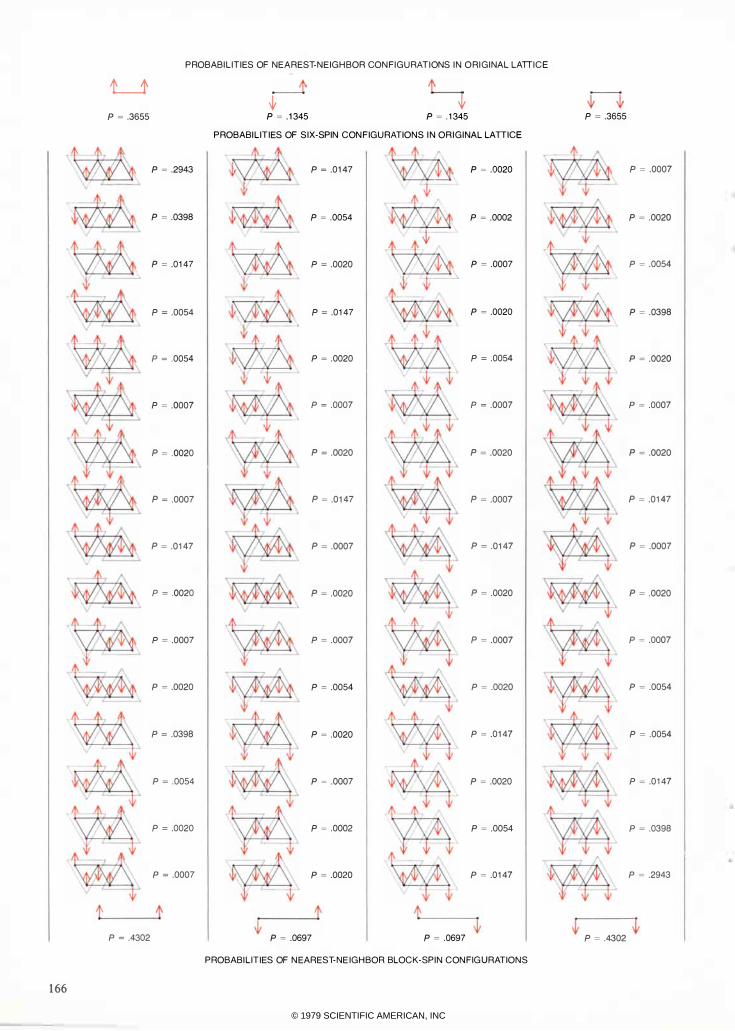
PROBABILITY DISTRIBUTION for a system of block spins is found by adding up the prob­abilities for all the configurations of the original lattice that contribute to each configuration of the block spins. The calculation is shown for a system of six spins on a triangular lattice. Two blocks of three spins each are formed from the lattice, and each block is replaced by a sin­gle spin whose orientation is determined by majority rule. The six spins have 64 possible config­urations, which are assigned to columns in such a way that all the configurations in each col­umn give rise to the same block-spin configuration. For example, all the configurations in the column at the far left have at least two spins in each block pointing up, so that they are rep­resented by two up block spins. The coupling strength in the original lattice is set equal to .5, which yields the nearest-neighbor probabilities shown at the top of the page. From this set of numbers a probability is calculated for every configuration of the original lattice; then all the probabilities in each colum n are added up to give the probability of the corresponding block­spin configuration. The block-spin probabilities are not the sam e as those specified for the orig­inal lattice, which im plies that the coupling strength is also d�fferent, as is the temperature.

given by the parameter K. the recipro­cal of the temperature.

This guess can easily be checked, be­cause the probability distribution for the configurations of at least a small part of the block-spin system is already known; it was computed from the con­figurations of the original lattice in the course of defining the block spins. S ur­prisingly, this hypothesis i s generally wrong: the block spins do not have the same couplings as the spins in the orig­inal model. Assuming that only adja­cent sites interact and that they have a coupling strength equal to K gives the wrong set of probabilities for the config­urations of the block spins.

I f the specifications of the original model will not describe the system of

block spins, then some new set of cou­plings m ust be invented. The g uiding principle in formulating these new inter­actions is to reproduce as accurately as possible the observed probability d istri­b ution. In general the nearest-neighbor coupling strength must be changed, that is, K m ust take on a new value. What is more, couplings of longer range, which were excluded by definition from the Ising model, m ust be introduced. For ex­ample, it may be necessary to establish a coupling between spins at the opposite corners of a square. There might also be direct interactions among spins taken three at a time or four at a time. Cou­plings of still longer range are possible. Hence the block spins can be regarded as a lattice system, but it is a system quite d ifferent from the original one. Notably, because the basic couplings have d ifferent values, the lattice of block spins is at a temperature d ifferent from that of the initial Ising system.

Once a set of couplings has been found that correctly describes the prob­ability d istr ibution for the block spins, a lattice of arbitrary size can be construct­ed from them. The new lattice is formed the same way the original one was, but now the probability for the spin at each site is determined by the newly derived coupling strengths rather than by the single coupling of the Ising model. The renormalization-group calculation now proceeds by starting all over again, with the new system of block spins as the starting lattice. Once again blocks of nine spins each are formed, and in some small region, s uch as an array of 36 spins, the probability of every possible configuration is found. This calc ulation is then employed to define the probabil­ity distribution of a second generation of block spins, which are once more formed by majority rule. Examination of the second-generation block spins shows that the couplings have again changed, so that new values must be s upplied a second time for each cou­pling strength. Once the new val ues have been determined another lattice system (the third generation) can be construct-

167

© 1979 SCIENTIFIC AMERICAN, INC

ed and the entire procedure can be re­peated yet again.

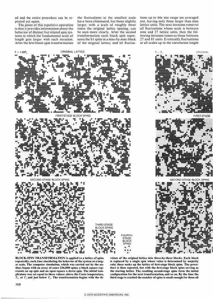
The point of this repetitive operation is that it provides information about the behavior of distinct but related spin sys­tems in which the fundamental scale of length gets larger with each iteration. After the first block-spin transformation

the fluctuations at the smallest scale have been eliminated, but those slightly larger, with a scale of roughly three times the original lattice spacing, can be seen more clearly. After the second transformation each block spin repre­sents the 8 1 spins in a nine-by-nine block of the original lattice, and all fluctua-

T = 1 .22Tc O R I G I NAL LATTICE

FIRST-STAGE BLOCK S P I N S

SECOND-STAGE BLOCK S P I N S

THI RD-STAGE BLOCK S P I N S

FOU RTH­STAGE BLOCK S P I N S

l.-<- JII -. �-=�� ;�.+,

tions up to this size range are averaged out, leaving only those larger than nine lattice units. The next iteration removes all fluctuations whose scale is between nine and 27 lattice units, then the fol­lowing iteration removes those between 27 and 8 1 units. Eventually fluctuations at all scales up to the correlation length

F I RST-STAGE

--

S ECOND -S TA G E BLOCK S P I N S

BLOCK-SPIN TRANSFORMATION is applied t o a lattice o f spins repeatedly, each time elucidating the behavior of the system at a larg­er scale. The computer simulation, which was carried out by the au­thor, began with an array of some 236,000 spins; a black square rep­resents an up spin and an open square a down spin. The initial tem­p�rature was set equal to three values: above the Curie temperature, Te. at Te and just below Te. The transformation begins with the di-

vision of the original lattice into three-by-three blocks. Each block is replaced by a single spin whose value is determined by majority rule; these make up the lattice of first-stage block spins. The proce­dure is then repeated, but with the first-stage block spins serving as the starting lattice. The resulting second-stage spins form the initial configuration for the next transformation, and so on. By the time the third stage is reached the number of spins is small enough for them all

1 68

© 1979 SCIENTIFIC AMERICAN, INC

LATIICE

are averaged out. The resulting spin sys­tem reflects only the long-range proper­ties of the original Ising system, with all finer-scale fluctuations eliminated.

The value of the block-spin technique can be perceived even through a simple visual inspection of the evolving model. Merely looking at a configuration of

�1TTTTH u.:..:-::: f::::: U u.::r. . . . . . ....... . .J!I!I�..... . __ � �_IIL-..UI • • J..'------.I..IJ!I�J!I�� •• �_ • • •• . . . . . . . . ... . . ... . .. • ..IL�_ •••• --.--.1i • • . . . . . . . . . . . . . . . . .. . . . . . .

BLOCK SPINS

___ 1 1 . 1 • • b M=- _

II II 'ftI.It:I

i 1: Ii

THIRD -STAGE BLOCK SPINS

FOU RTH­STAGE BLOCK SPINS

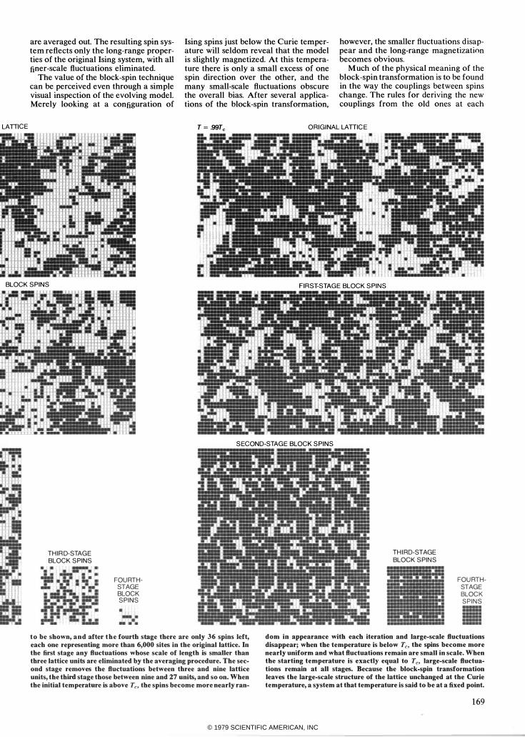
Ising spins just below the Curie temper­ature will seldom reveal that the model is slightly magnetized. At this tempera­ture there is only a small excess of one spin direction over the other, and the many small-scale fluctuations obscure the overall bias_ After several applica­tions of the block-spin transformation,

however, the smaller fluctuations disap­pear and the long-range magnetization becomes obvious.

M uch of the physical meaning of the block-spin transformation is to be found in the way the couplings between spins change. The rules for deriving the new couplings from the old ones at each

T = .99Tc ORIGINAL LATIICE

FIRST-STAGE BLOCK SPINS

SECOND-STAGE BLOCK SPINS

THI RD -STAGE BLOCK SPINS

FOU RTH­STAGE BLOCK S P I N S

t o be shown, a n d after t h e fourth stage there are only 3 6 spins left, each one representing more than 6,000 sites in the original lattice. In the first stage any fluctuations whose scale of length is smaller than three lattice units are eliminated by the averaging procedure. The sec­ond stage removes the fluctuations between three and nine lattice units, the third stage those between nine and 27 nnits, and so on. When the initial temperature is above Te, the spins become more nearly ran-

dom in appearance with each iteration and large-scale fluctuations disappear; when the temperature is below Te, the spins become more nearly uniform and what fluctuations remain are small in scale. When the starting temperature is exactly equal to Te. large-scale fluctua­tions remain at all stages. Because the block-spin transformation leaves the large-scale structure of the lattice unchanged at the Curie temperature, a system at that temperature is said to be at a fixed point.

1 69

© 1979 SCIENTIFIC AMERICAN, INC

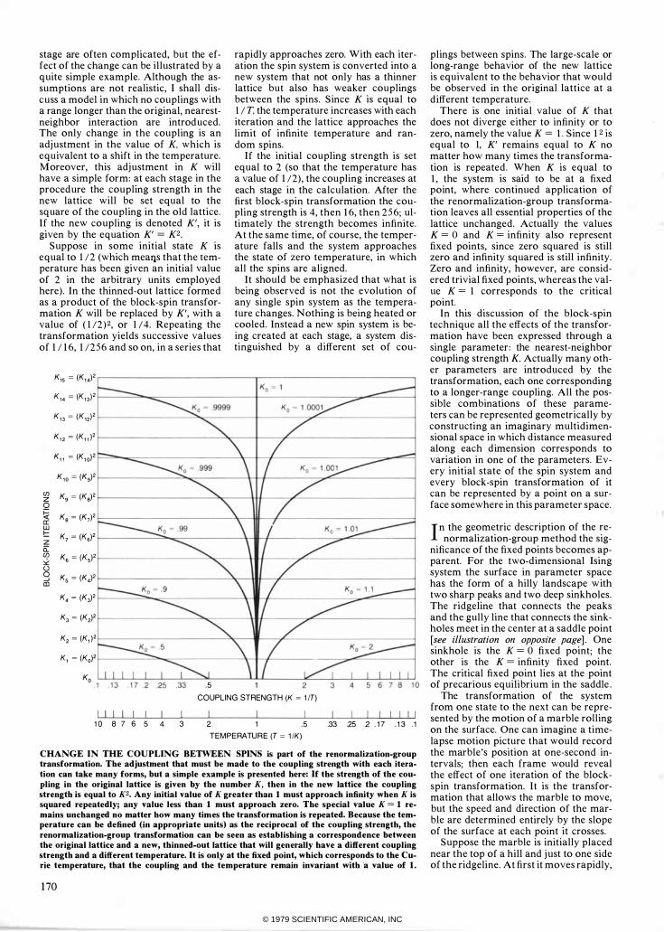
stage are often complicated, but the ef­fect of the change can be i l lustrated by a quite simple example. Although the as­sumptions are not realistic, I shall dis­cuss a model in which no couplings with a range longer than the original, nearest­neighbor interaction are introd uced. The only change in the coupling is an adj ustment in the value of K. which is equivalent to a shift in the temperature. Moreover, this adj ustment in K will have a simple form: at each stage in the procedure the coupling strength in the new lattice will be set equal to the sq uare of the coupling in the old lattice. If the new coupling is denoted K', it is given by the equation K' = K2 .

Suppose in some initial state K is eq ual to 1 / 2 (which mealls that the tem­perature has been given an initial value of 2 in the arbitrary units employed here). In the thinned-out lattice formed as a product of the block-spin transfor­mation K will be replaced by K', with a value of ( 1 /2 ) 2, or 1 / 4. Repeating the transformation yields successive values of 1 / 1 6, 1 / 2 5 6 and so on, in a series that

K15 = (K' 4)'

K14 = (K,, ) '

K ' 3 = (K,,)'

K" = (K, , )'

K" = (Kl O)'

K,o = (Kg)'

(f) Kg = (K.)' z 0 � K. = (K,)' a: w t::: K, = (K.)' z a: (f) K. = (Ks)' � u 0 Ks = (K4)' -' CD

K4 = (K3)'

K3 = (K,)'

K, = (K, )'

K, = (Ko)'

Ko

rapidly approaches zero. With each iter­ation the spin system is converted into a new system that not only has a thinner lattice but also has weaker couplings between the spins. S ince K is equal to 1 / T, the temperature increases with each iteration and the lattice approaches the limit of infinite temperature and ran­dom spins.

I f the initial coupling strength is set equal to 2 (so that the temperature has a value of 1 / 2) , the coupling increases at each stage in the calculation. After the first block-spin transformation the cou­pling strength is 4, then 1 6, then 2 5 6; ul­timately the strength becomes infinite. At the same time, of course, the temper­ature falls and the system approaches the state of zero temperature, in which all the spins are aligned.

I t should be emphasized that what is being observed is not the evolution of any single spin system as the tempera­ture changes. Nothing is being heated or cooled . Instead a new spin system is be­ing created at each stage, a system dis­tinguished by a d ifferent set of cou-

. 5 1

I I I I I 1 0 8 7 6 5 4 3

COUPLING STRENGTH (K = 1 /T)

2 1 , 5 TEMPERATU R E (T = 1 1K)

I I I I I ,33 .25 ,2 . 1 7 .13 .1

CHANGE IN THE COUPLING BETWEEN SPINS is part of the renormalization-group transformation. The adjustment that must be made to the coupling strength with each itera­tion can take many forms, but a simple example is presented here: If the strength of the cou­pling in the original lattice is given by the number K, then in the new lattice the coupling strength is equal to K2. Any initial value of K greater than 1 must approach infinity when K is squared repeatedly; any value less than 1 must approach zero. The special value K = 1 re­mains unchanged no matter how many tim es the transformation is repeated. Because the tem­perature can be defined (in appropriate units) as the reciprocal of the coupling strength, the renormalization-group transformation can be seen as establishing a correspondence between the original lattice and a new, thinned-out lattice that will generally have a different coupling strength and a different temperature. It is only at the fixed point, which corresponds to the Cu­rie temperature, that the coupling and the temperature remain invariant with 'a value of 1 .

1 70

plings between spins. The large-scale or long-range behavior of the new lattice is equivalent to the behavior that would be observed in the original lattice at a d ifferent temperature.

There is one initial value of K that does not diverge either to infinity or to zero, namely the value K = 1 . S ince 1 2 is equal to I, K' remains equal to K no matter how many times the transforma­tion is repeated. When K is equal to 1 , the system is said to be at a fixed point, where continued application of the renormalization-group transforma­tion leaves all essential properties of the lattice unchanged. Actually the values K = 0 and K = infinity also represent fixed points, since zero squared is still zero and infinity squared is still infinity. Zero and infinity, however, are consid­ered trivial fixed points, whereas the val­ue K = 1 corresponds to the critical point.

In this discussion of the block-spin technique all the effects of the transfor­mation have been expressed through a single parameter : the nearest-neighbor coupling strength K. Actually many oth­er parameters are introduced by the transformation, each one corresponding to a longer-range coupling. All the pos­sible combinations of these parame­ters can be represented geometrically by constructing an imaginary multidimen­sional space in which d istance measured along each d imension corresponds to variation in one of the parameters. Ev­ery initial state of the spjn system and every block-spin transformation of it can be represented by a point on a sur­face somewhere in this parameter space.

In the geometric description of the re­normalization-group method the sig­

nificance of the fixed points becomes ap­parent. For the two-dimensional Ising system the surface in parameter space has the form of a hilly landscape with two sharp peaks and two deep sinkholes. The ridgeline that connects the peaks and the gully line that connects the sink­holes meet in the center at a saddle point [see illustration on opposite page] . One sinkhole is the K = 0 fixed point; the other is the K = infinity fixed point. The critical fixed point lies at the point of precarious equilibrium in the saddle .

The transformation of the system from one state to the next can be repre­sented by the motion of a marble rolling on the surface. One can imagine a time­lapse motion picture that would record the marble's position at one-second in­tervals; then each frame would reveal the effect of one iteration of the block­spin transformation. I t is the transfor­mation that allows the marble to move, but the speed and direction of the mar­ble are determined entirely by the slope of the surface at each point it crosses.

Suppose the marble is initially placed near the top of a hill and j ust to one side of the ridgeline. At first it moves rapidly,

© 1979 SCIENTIFIC AMERICAN, INC

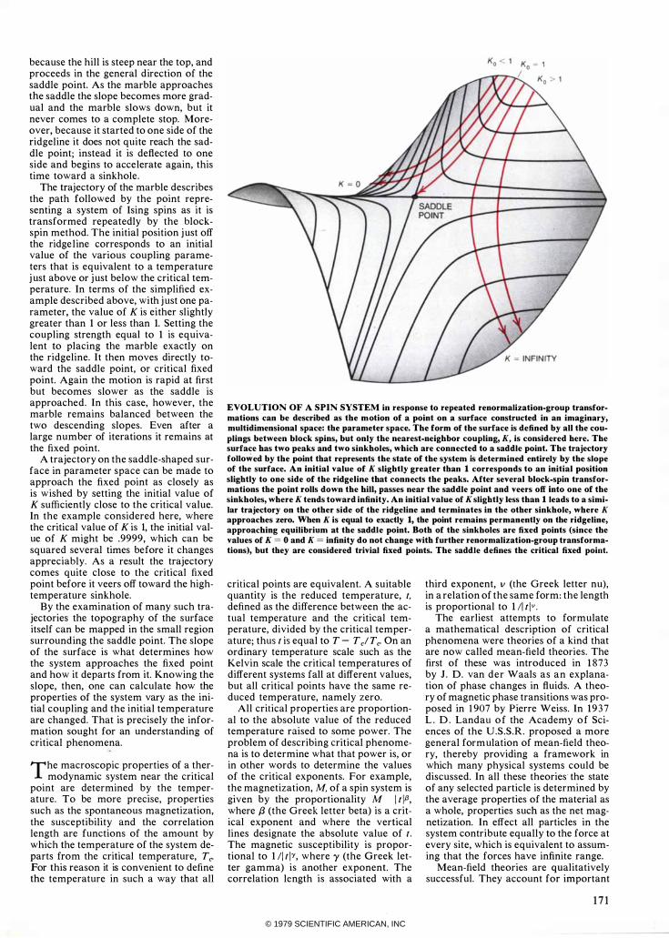
because the hill is steep near the top, and proceeds in the general direction of the saddle point. As the marble approaches the saddle the slope becomes more grad­ual and the marble slows down, but it never comes to a complete stop. More­over, because it started to one side of the ridgeline it does not quite reach the sad­dle point; instead it is deflected to one side and begins to accelerate again, this time toward a sinkhole .

The trajectory of the marble describes the path followed by the point repre­senting a system of Ising spins as it is transformed repeatedly by the block­spin method. The initial position j ust off the ridge l ine corresponds to an initial value of the various coupling parame­ters that is equivalent to a temperature j ust above or j ust below the critical tem­perature. In terms of the simplified ex­ample described above, with j ust one pa­rameter, the value of K is either sl ightly greater than 1 or less than 1. Setting the coupling strength equal to 1 is equiva­lent to placing the marble exactly on the ridgeline. It then moves directly to­ward the saddle point, or critical fixed point. Again the motion is rapid at first but becomes slower as the saddle is approached. In this case, however, the marble remains balanced between the two descending slopes. Even after a large number of iterations it remains at the fixed point.

A trajectory on the saddle-shaped sur­face in parameter space can be made to approach the fixed point as closely as is wished by setting the initial value of K sufficiently close to the critical value. In the example considered here, where the critical value of K is 1, the initial val­ue of K might be .9999, which can be squared several times before it changes appreciably. As a result the trajectory comes quite close to the critical fixed point before it veers off toward the high­temperature sinkhole.

By the examination of many such tra­jectories the topography of the surface itself can be mapped in the small region surrounding the saddle point. The slope of the surface is what determines how the system approaches the fixed point and how it departs from it. Knowing the slope, then, one can calculate how the properties of the system vary as the ini­tial coupling and the initial temperature are changed. That is precisely the infor­mation sought for an understanding of critical phenomena. .

The macroscopic properties of a ther­modynamic system near the critical

point are determined by the temper­ature. To be more precise, properties such as the spontaneous magnetization, the susceptibility and the correlation length are functions of the amount by which the temperature of the system de­parts from the critical temperature, Te• For this reason it is convenient to define the temperature in such a way that all

EVOLUTION OF A SPIN SYSTEM in response to repeated renormalization-group transfor­mations can be described as tbe motion of a point on a surface constructed in an imaginary, multidimensional space: tbe parameter space. Tbe form of tbe surface is defined by all tbe con­plings between block spins, but only tbe nearest-neigbbor coupling, K, is considered bere. Tbe surface bas two peaks and two sinkboles, wbicb are connected to a saddle point. Tbe trajectory followed by tbe point tbat represents tbe state of tbe system is determined entirely by tbe slope of tbe surface. An initial value of K sligbtly greater tban 1 corresponds to an initial position sligbtly to one side of tbe ridgeline tbat connects tbe peaks. After several block-spin transfor­mations tbe point rolls down tbe bill, passes near tbe saddle point and veers off into one of tbe sinkboles, wbere K tends toward infinity. An initial value of K sligbtly less tban 1 leads to a simi­lar trajectory on tbe otber side of tbe ridgeline and terminates in tbe otber sinkbole, wbere K approacbes zero. Wben K is equal to exactly 1, tbe point remains permanently on tbe ridgeline, approacbing equilibrium at tbe saddle point. Botb of tbe sinkboles are fixed points (since tbe values of K = 0 and K = infinity do not cbange witb furtber renormalization-group transforma­tions), but tbey are considered trivial fixed points. Tbe saddle defines tbe critical fixed point.

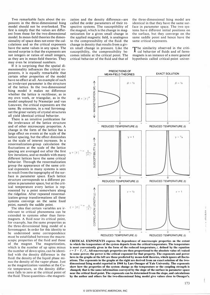
critical points are equivalent. A suitable quantity is the reduced temperature, t, defined as the difference between the ac­tual temperature and the critical tem­perature, divided by the critical temper­ature; thus t is equal to T - Tel Te. On an ordinary temperature scale such as the Kelvin scale the critical temperatures of different systems fall at different values, but all critical points hav'e the same re­duced temperature, namely zero.

All critical properties are proportion­al to the absolute value of the reduced temperature raised to some power. The problem of describing critical phenome­na is to determine what that power is, or in other words to determine the values of the critical exponents. For example, the magnetization, M, of a spin system is given by the proportionality M I t ill, where {3 (the Greek letter beta) is a crit­ical exponent and where the vertical lines designate the absolute value of t. The magnetic susceptibility is propor­tional to 1 II f lY, where 'Y (the Greek let­ter gamma) is another exponent. The correlation length is associated with a

third exponent, v (the Greek letter nu), in a relation of the same form: the length is proportional to 1 /1 t l v .

The earliest attempts to formulate a mathematical description of critical phenomena were theories of a kind that are now called mean-field theories. The first of these was introduced in 1 873 by J . D. van der Waals as an explana­tion of phase changes in fluids. A theo­ry of magnetic phase transitions was pro­posed in 1 907 by Pierre Weiss. In 1 9 3 7 L . D . Landau o f the Academy o f Sci­ences of the U.S .S .R. proposed a more general formulation of mean-field theo­ry, thereby providing a framework in which many physical systems could be discussed. In all these theories' the state of any selected particle is determined by the average properties of the material as a whole, properties such as the net mag­netization. In effect all particles in the system contribute equally to the force at every site, which is equivalent to assum­ing that the forces have infinite range.

Mean-field theories are qualitatively successful. They account for important

17 1

© 1979 SCIENTIFIC AMERICAN, INC

Ko = 1.1

Ko = 1.01

Ko = 1.001

Ko = 1.0001

Ko = 1

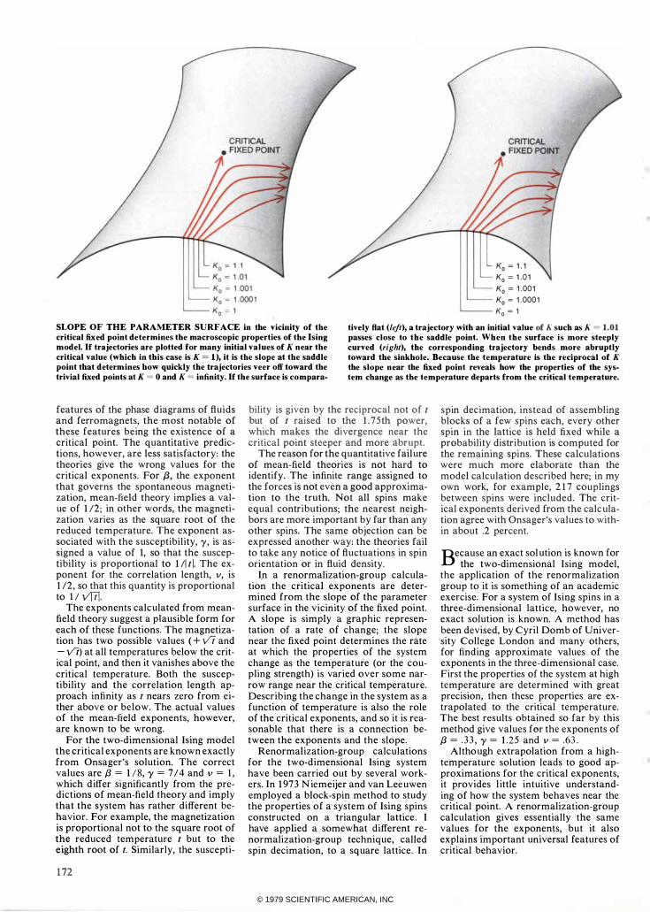
SLOPE OF THE PARAMETER SURFACE in tbe vicinity of the critical fixed point determines tbe macroscopic properties of the Ising model. If trajectories are plotted for many initial values of K near the critical value (wbicb in tbis case is K = 1 ), it is the slope at the saddle point tbat determ ines bow quickly tbe trajectories veer off toward the trivial fixed points at K = 0 and K = infinity. If tbe surface is com para-

tively flat (/e!t), a trajectory witb an initial value of K sucb as K = 1.01 passes close to tbe saddle point. Wben tbe surface is more steeply curved (right), tbe corresponding trajectory bends more abruptly toward tbe sinkbole. Because tbe temperature is tbe reciprocal of K tbe slope near tbe fixed point reveals bow tbe properties of tbe sys­tem change as the temperature departs from the critical temperature.

features of the phase d iagrams of fluids and ferromagnets, the most notable of these features being the existence of a critical point. The quantitative predic­tions, however, are less satisfactory: the theories give the wrong values for the critical exponents. For {3, the exponent that governs the spontaneous magneti­zation, mean-field theory implies a val­ue of 1 12; in other words, the magneti­zation varies as the square root of the reduced temperature. The exponent as­sociated with the susceptibility, 'Y, is as­signed a value of 1, so that the suscep­tibility is proportional to 1 /1 1 1. The ex­ponent for the correlation length, v, is 1 12 , so that this quantity is proportional to 1 / vTtl,

The exponents calculated from mean­field theory suggest a plausible form for each of these functions. The magnetiza­tion has two possible values ( + Vi and - Vi) at all temperatures below the crit­ical point, and then it vanishes above the critical temperature. Both the suscep­tibility and the correlation length ap­proach infinity as 1 nears zero from ei­ther above or below. The actual values of the mean-field exponents, however, are known to be wrong.

For the two-dimensional Ising model the critical exponents are known exactly from Onsager's solution. The correct values are {3 = 1 / 8, 'Y = 7 / 4 and v = I , which d iffer significantly from the pre­dictions of mean-field theory and imply that the system has rather different be­havior. For example, the magnetization is proportional not to the square root of the reduced temperature 1 but to the eighth root of f. Similarly, the suscepti-

172

bility is given by the reciprocal not of 1 but of 1 raised to the 1 . 75th power, which makes the divergence near the critical point steeper and more abrupt.

The reason for the quantitative failure of mean-field theories is not hard to identify. The infinite range assigned to the forces is not even a good approxima­tion to the truth. Not all spins make equal contributions; the nearest neigh­bors are more important by far than any other spins. The same objection can be expressed another way: the theories fail to take any notice of fluctuations in spin orientation or in fluid density.

I.n a renormalization-group calcula­tion the critical exponents are deter­mined from the slope of the parameter surface in the vicinity of the fixed point. A slope is simply a graphic represen­tation of a rate of change; the slope near the fixed point determines the rate at which the properties of the system change as the temperature (or the cou­pling strength) is varied over some nar­row range near the critical temperature. Describing the change in the system as a function of temperature is also the role of the critical exponents, and so it is rea­sonable that there is a connection be­tween the exponents and the slope.

Renormalization-group calculations for the two-dimensional Ising system have been carried out by several work­ers. In 1 973 N iemeijer and van Lee uwen employed a block-spin method to study the properties of a system of Ising spins constructed on a triangular lattice . I have applied a somewhat different re­normalization-group technique, called spin decimation, to a square lattice . In

spin decimation, instead of assembling blocks of a few spins each, every other spin in the lattice is held fixed while a probability distribution is computed for the remaining spins. These calculations were much more elaborate than the model calculation described here; in my own work, for example, 2 1 7 couplings between spins were included. The crit­ical exponents derived from the calc ula­tion agree with Onsager's values to with­in about .2 percent.

Because an exact sol ution is known for the two-dimensional Ising model,

the application of the renormalization group to it is something of an academic exercise. For a system of Ising spins in a three-dimensional lattice, however, no exact solution is known. A method has been devised, by Cyril Domb of Univer­sity College London and many others, for finding approximate values of the exponents in the three-dimensional case. First the properties of the system at high temperature are determined with great precision, then these properties are ex­trapolated to the critical temperature. The best results obtained so far by this method give values fer the exponents of {3 = . 3 3 , 'Y = 1 .2 5 and v = .63 .

Altho ugh extrapolation from a high­temperature solution leads to good ap­proximations for the critical exponents, it provides l ittle intuitive understand­ing of how the system behaves near the critical point. A renormalization-group calculation gives essentially the same values for the exponents, but it also explains important universal features of critical behavior.

© 1979 SCIENTIFIC AMERICAN, INC

Two remarkable facts about the ex­ponents in the three-dimensional Ising model should not be overlooked. The first is simply that the values are differ­ent from those for the two-dimensional model. In mean-field theories the dimen­sional ity of space does not enter the cal­c ulations and so the critical exponents have the same values in any space. The second surprise is that the exponents are not integers or ratios of small integers, as they are in mean-field theories. They may even be irrational numbers.

If it is surprising that the spatial di­mensionality infl uences the critical ex­ponents, it is equally remarkable that certain other properties of the model have no effect at all . An example of such an irrelevant parameter is the structure of the lattice. In the two-dimensional Ising model it makes no difference whether the lattice is rectilinear, as in my own work, or triangular, as in the model employed by N iemeijer and van Leeuwen; the critical exponents are the same. By extension, in a real ferromag­net the great variety of crystal structures all yield identical critical behavior .

There is an intuitive j ustification for the irrelevance of the lattice structure and of other microscopic properties. A change in the form of the lattice has a large effect on events at the scale of the lattice spacing, but the effect diminishes as the scale of interest increases. In a renormalization-group calculation the fl uctuations at the scale of the lattice spacing are averaged out after the first few iterations, and so models with many different lattices have the same critical behavior. Through the renormalization group the appearance of the same crit­ical exponents in many systems is seen to result from the topography of the sur­face in parameter space. Each lattice structure corresponds to a different po­sition in parameter space, but at the crit­ical temperature every lattice is rep­resented by a point somewhere along the ridgeline. After repeated renormal­ization-group transformations all these systems converge on the same fixed point, namely the saddle point.

The idea that certain variables are ir­relevant to critical phenomena can be extended to systems other than ferro­magnets. A fluid near its critical point, for example, has the same properties as the three-dimensional Ising model of a ferromagnet. In order for this identity to be understood some correspondence m ust be establ ished between the macro­scopic properties of the fl uid and those of the magnet. The magnetization, which is the number of up spins minus the number of down spins, can be identi­fied with the density difference in the fluid : the density of the liquid phase mi­nus the density of the vapor phase . J ust as the magnetization vanishes at the Cu­rie temperature, so the density d iffer­ence falls to zero at the critical point of the fluid. These q uantities-the magnet i-

zation and the density difference-are called the order parameters of their re­spective systems. The susceptibility of the magnet, which is the change in mag­netization for a given small change in the applied magnetic field, is analogous to the compressibility of the fluid : the change in density that results from a giv­en small change in pressure. Like the s usceptibility, the compressibility be­comes infinite at the critical point. The critical behavior of the fluid and that of

the three-dimensional Ising model are identical in that they have the same sur­face in parameter space. The two sys­tems have different initial positions on the surface, but they converge on the same saddle point and hence have the same critical exponents.

The similarity observed in the criti­cal behavior of fluids and of ferro­

magnets is an instance of a more general hypothesis called critical-point univer-

PREDICTIONS OF

MEAN-FIELD THEORIES EXACT SOLUTION

o + REDUCED TEMPERATURE (t)

y = 1

o REDUCED TEMPERATURE (t)

v = V2

+ -

--..... ./

{3 = VB

o + REDUCED TEMPERATURE (t)

o + REDUCED TEMPERATURE (t)

v = 1

o + - 0 + REDUCED TEMPE RATURE (t) REDUCED TEMPE RATURE (t)

CRITICAL EXPONENTS express the dependence of macroscopic properties on the extent to which the temperature of the system departs from the critical temperature. The temperature is most conveniently given in the form of the reduced temperature, I, defined by the equation I = T - Tel Te. All macroscopic properties are then proportional to the absolute value of t raised to some power; the power is the critical exponent for that property. The exponents and power laws in the graphs at the left are those predicted by m ean-field theories, which ignore all fluctu­ations. The exponents in the graphs at the right are derived from an exact solution of the two­dim ensional Ising m odel reported in 1944 by Lars Onsager of Yale University. The exponents show how the properties of the system change as the temperature or the coupling strength is changed; that is the sam e information conveyed by the slope of the surface in parameter space near the critical fixed point. The exponents can be determined from the slope, and calculations by the author and others for the two-dim ensional Ising model give values close to Onsager!s.

1 73

© 1979 SCIENTIFIC AMERICAN, INC

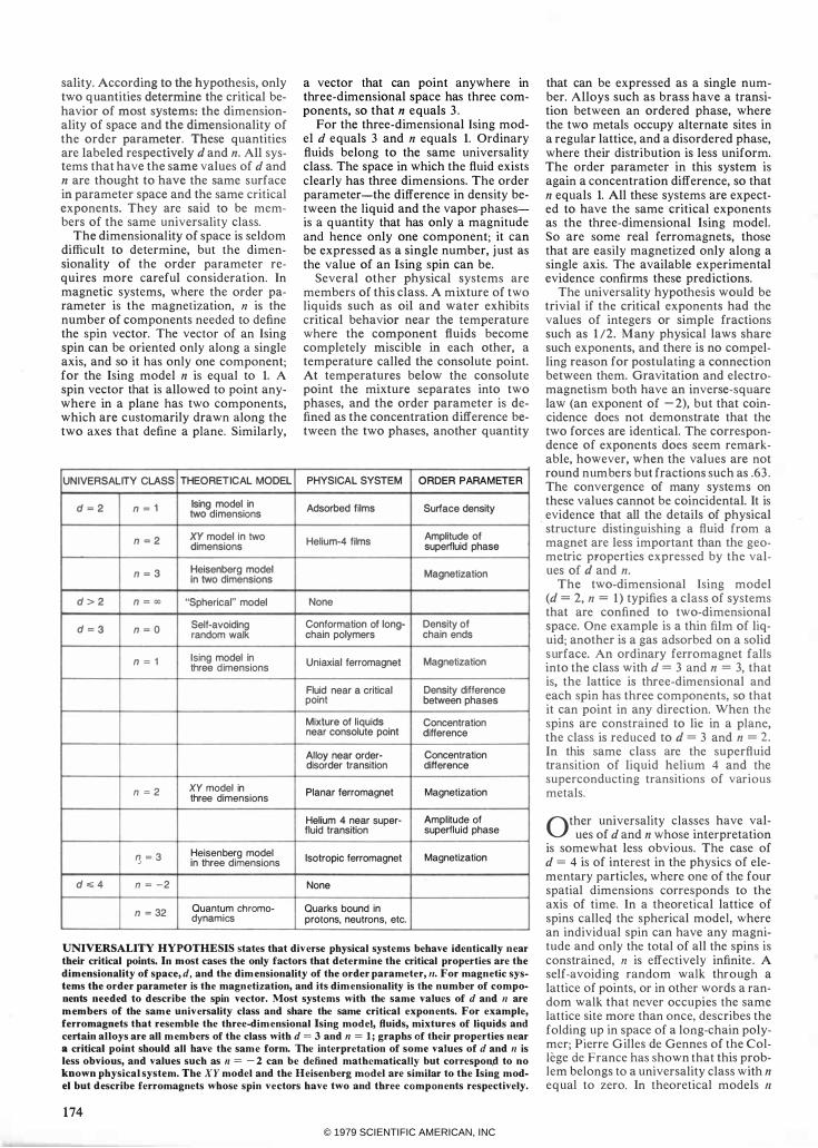
sality. According to the hypothesis, only two quantities determine the critical be­havior of most systems: the dimension­ality of space and the dimensionality of the order parameter. These quantities are labeled respectively d and n. All sys­tems that have the same values of d and n are thought to have the same surface in parameter space and the same critical exponents. They are said to be mem­bers of the same universality class.

The dimensionality of space is seldom difficult to determine, but the dimen­sionality of the order parameter re­quires more careful consideration. In magnetic systems, where the order pa­rameter is the magnetization, n is the number of components needed to define the spin vector. The vector of an Ising spin can be oriented only along a single axis, and so it has only one component; for the Ising model n is equal to 1. A spin vector that is allowed to point any­where in a plane has two components, which are customarily drawn along the two axes that define a plane. Similarly,

UNIVERSALITY CLASS THEORETICAL MODEL

d = 2 n = 1 Ising model in two dimensions

n = 2 XY model in two dimensions

n = 3 Heisenberg model in two dimensions

d > 2 n = oo "Spherical" model

d = 3 n = O Self·avoiding random walk

n = 1 Ising model in three d imensions

n = 2 XY model in three dimensions

� = 3 Heisenberg model in three dimensions

d ,,;; 4 n = -2 n = 32 Quantum chromo·

dynamics

a vector that can point anywhere in three-dimensional space has three com­ponents, so that n equals 3 .

For the three-dimensional Ising mod­el d equals 3 and n equals 1. Ordinary fluids belong to the same universality class. The space in which the fluid exists clearly has three dimensions. The order parameter-the difference in density be­tween the liquid and the vapor phases­is a quantity that has only a magnitude and hence only one component; it can be expressed as a single number, j ust as the value of an Ising spin can be.

Several other physical systems are members of this class. A mixture of two liquids such as oil and water exhibits critical behavior near the temperature where the component fluids become completely miscible in each other, a temperature called the consolute point. At temperatures below the consolute point the mixture separates into two phases, and the order parameter is de­fined as the concentration difference be­tween the two phases, another quantity

PHYSICAL SYSTEM ORDER PARAMETER

Adsorbed films Surface density

Helium-4 films Amplitude of superfluid phase

Magnetization

None

Conformation of long- Density of chain polymers chain ends

Uniaxial ferromagnet Magnetization

Fluid near a critical Density difference point between phases

Mixture of l iquids Concentration near consolute point difference

Alloy near order- Concentration disorder transition difference

Planar ferromagnet Magnetization

Helium 4 near super· Amplitude of fluid transition superfluid phase

Isotropic ferromagnet Magnetization

None

Quarks bound in protons, neutrons, etc.

UNIVERSALITY HYPOTHESIS states that diverse physical systems behave identically near their critical points. In most cases the only factors that determine the critical properties are the dimensionality of space, d, and the dim ensionality of the order parameter, 11. For magnetic sys­tems the order parameter is the magnetization, and its dim ensionality is the number of compo­nents needed to describe the spin vector. Most systems with the same values of d and 11 are m embers of the sam e universality class and share the same critical expon ents. For example, ferromagnets that resemble the three-dim ensional Ising model, fluids, mixtures of liquids and certain alloys are all m embers of the class with d = 3 and 11 = 1; graphs of their properties near a critical point should all have the sam e form. The interpretation of some values of d and 11 is less obvious, and values such as 11 = - 2 can be defined mathematically but corresponft to no known physical system. The XY model and the Heisenberg model are similar to the Ising mod­el but describe ferromagnets whose spin vectors have two and three components respectively.

1 74

that can be expressed as a single num­ber. Alloys such as brass have a transi­tion between an ordered phase, where the two metals occupy alternate sites in a regular lattice, and a disordered phase, where their distribution is less uniform. The order parameter in this system is again a concentration difference, so that n equals 1. All these systems are expect­ed to have the same critical exponents as the three-dimensional Ising model. So are some real ferromagnets, those that are easily magnetized only along a single axis. The available experimental evidence confirms these predictions.

The universality hypothesis would be trivial if the critical exponents had the values of integers or simple fractions such as 1 12. Many physical laws share such exponents, and there is no compel­ling reason for postulating a connection between them. Gravitation and electro­magnetism both have an inverse-square law (an exponent of - 2), but that coin­cidence does not demonstrate that the two forces are identical. The correspon­dence of exponents does seem remark­able, however, when the values are not round numbers but fractions such as .63 . The convergence of many systems on these values cannot be coincidental. It is evidence that all the details of physical

, structure distinguishing a fluid from a magnet are less important than the geo­metric plOperties expressed by the val­ues of d and n.

The two-dimensional Ising model (d = 2, n = 1 ) typifies a class of systems that are confined to two-dimensional space. One example is a thin film of liq­uid; another is a gas adsorbed on a solid surface. An ordinary ferromagnet falls into the class with d = 3 and n = 3, that is, the lattice is three-dimensional and each spin has three components, so that it can point in any direction. When the spins are constrained to lie in a plane, the class is reduced to d = 3 and n = 2 . In this same class are the superfluid transition of liquid helium 4 and the superconducting transitions of various metals.

Other universality classes have val­ues of d and n whose interpretation

is somewhat less obvious. The case of d = 4 is of interest in the physics of ele­mentary particles, where one of the four spatial dimensions corresponds to the axis of time. In a theoretical lattice of spins callee! the spherical model, where an individual spin can have any magni­tude and only the total of all the spins is constrained, n is effectively infinite . A self·avoid ing random walk through a lattice of points, or in other words a ran­dom walk that never occupies the same lattice site more than once, describes the folding up in space of a long-chain poly­mer; Pierre G illes de Gennes of the Col­lege de France has shown that this prob­lem belongs to a universality class with n equal to zero, In theoretical models n

© 1979 SCIENTIFIC AMERICAN, INC

Garden m� �lores the obvious and the obscure, the how-to and the how-cortJe, the superstition and the sQence of bOtany, horticul­ture, floriculture, agriculture and the environment. A gift of year-round entertainment for the enterprising and inquisitive gardener.

A Garden sampler: 'the Spiderwort Assay: A Japanese plant geneticist has develoPed clones of a wildflower that can detect ioniz­ing radiation with more sensitivity than a Geiger counter.

The Bamboozling Thamnocalamus: ' In synchronization throulrltout the world, a popular garden bamboo is blooming for the first time in a century -signaling the death of this entire

generation of the species. The Non-Lawn Grass: There is a beautiful natural alternative to turf that requires no mowing, spraying or fertilizing. Power Lines in the Wake of 2,4,5-T: There is a non-liZhemical alternative to the country's most toxic herbicide-'­currently used by utility companies to maintain fully 32,000 square miles of transmission line rights-of-way.

. The Directors of the Chicago Horti­cultural Society, The .Horticultural Society of New York, Los Angeles Arboretum and The New York Botanical Garden invite you to subscribe now at a cost of $10 for six bi-monthly, full-color issues.

I'''-�'-''-''-'�- ---::-�� - '''' ''- - --"-A-:� - �' -" - --�- l , Yes, start my subscription with a free current issue. I I enclose a $ 1 0 check ( $ 1 2 foreign) for six bi-monthly full-color issues. I Please send Garden to: I Name ____________________________________________ __ I I Address -----------------------------------------

Edition wanted: D Chicago Horticultural Society D Horticultural Society of New York D Los Angeles Arboretum Clip and mail to:

D New York Botanical Garden / Queens Botanical Garden

D No regional news, please

Subscription Department, Garden magazine, Botanical Garden , Bronx, N.Y. 1 0458

© 1979 SCIENTIFIC AMERICAN, INC

If you have ever taken a lux­ury sports car through a tight turn, you know the feeling. It's the sense of supreme pre­cision with which this trim, compact camera proclaims its N ikon heritage. A feeling that is borne out by the pro­fessional quality pictures the Nikon FE delivers with automatic ease. And one that, unlike other fine things in life, is readily affordable.

With the Nikon Ft;, you can simply focus and shoot . . . and rely on its Nikon elec­tronics to give you sharp, magnificently exposed photographs, automatically. Or, switch to manual opera­tion and enjoy complete creative control over every exposure, more easily than you ever thought possible.

Above all, this is a camera that makes no compromise in its supreme Nikon quality. Stroke the advance lever, and feel the smoothness of precision gearing machined to microscopic tolerances. Press the exposure button, and hear the shutter respond with hushed precision. Look through the bright, silver­coated viewfinder, and see your picture snap into sharp focus with a fingertip touch.

Know, too, that the world's greatest photographic sys­tem stands behind your Nikon FE. Add the dynamic firepower of motor drive, at up to 3. 5 shots a second. Banish darkness with the in­genious automatic thyristor flash. Explore new perspec­tives through more than 60 Nikkor lenses, the same superb optics chosen by most professionals for their sharpness and color fidelity.

For the purist: The Nikon FM For those who prefer only manual exposure control, the Nikon FM offers the reliable guidance of one-step elec­tronic metering. It's as com­pact and precisely responsive as the FE and costs even less. At your N ikon dealer.

Nikon Inc . • Garden City. New York 11530. In Canada : Nikon Canada. Inc. © Nikon Inc. 1979

fxperience a sense of perfection.

The Nikon ft:.

© 1979 SCIENTIFIC AMERICAN, INC

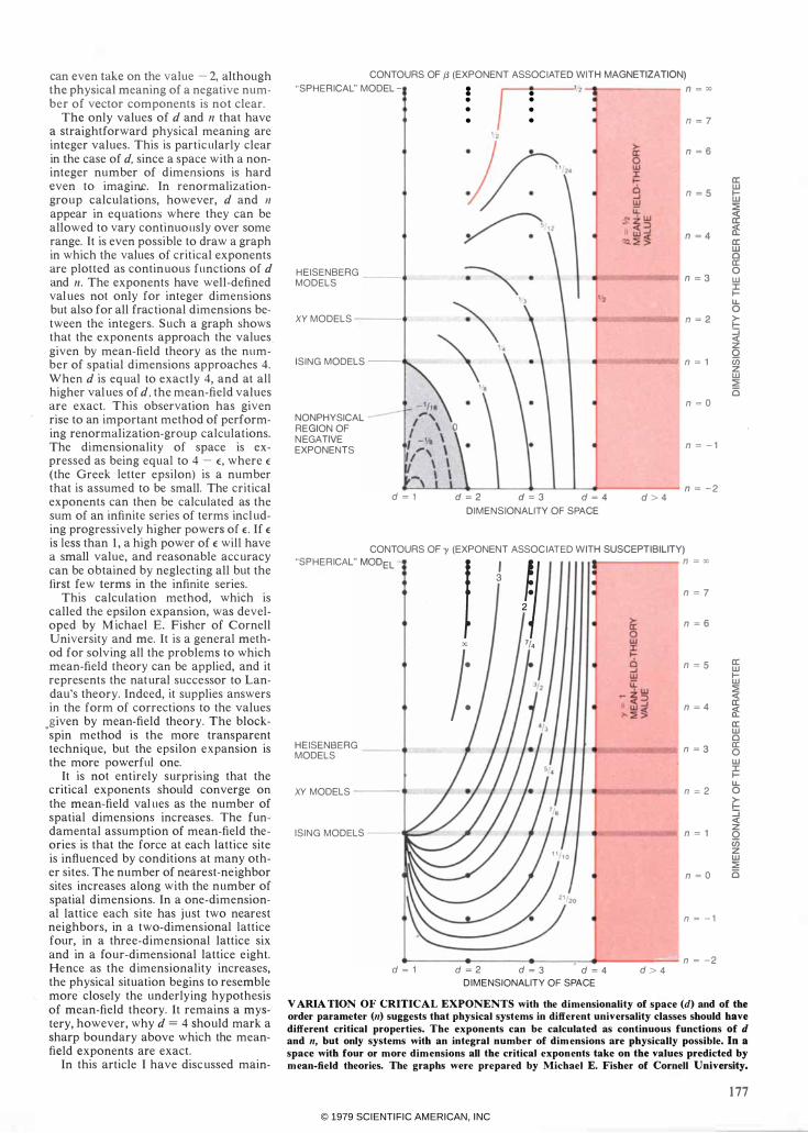
can even take on the value - 2, although the physical meaning of a negative num­ber of vector components is not clear.

The only values of d and /l that have a straightforward physical meaning are integer values. This is partic ularly clear in the case of d, since a space with a non­integer number of dimensions is hard even to imagint!. In renormalization­group calculat ions, however, d and /I appear in equations where they can be allowed to vary continuo usly over some range. It is even possible to draw a graph in which the values of critical exponents are plotted as contin uous functions of d and /l . The exponents have well-defined val ues not only for integer dimens ions but also for all fractional d imensions be­tween the integers. Such a graph shows that the exponents approach the values . given by mean-field theory as the num­ber of spatial d imensions approaches 4. When d is eq ual to exactly 4, and at all higher val ues of d, the mean-field values are exact. This observation has given rise to an important method of perform­ing renormalization-group calculations. The dimensionality of space is ex­pressed as being equal to 4 - E , where E ( the Greek letter epsilon) is a number that is assumed to be small. The critical exponents can then be calculated as the sum of an infinite series of terms incl ud­ing progressively higher powers of E . If E is less than I , a high power of E will have a small value, and reasonable accuracy can be obtained by neglect ing all but the first few terms in the infinite series.

This calculation method, which is called the epsilon expansion, was devel­oped by M ichael E. Fisher of Cornell University and me. It is a general meth­od for solving all the problems to which mean-field theory can be applied, and it represents the nat ural successor to Lan­dau's theory. Indced, it supplies answers in the form of corrections to the values

.given by mean-field theory. The block­spin method is the more transparent technique, but the epsilon e xpansion is the more powerful one.

It is not entirely surpris ing that the critical exponents should converge on the mean-field val ues as the number of spatial d imensions increases. The fun­damental assumption of mean-field the ­ories is that the force at each lattice site is influenced by conditions at many oth­er sites. The number of nearest-ne ighbor sites increases along with the number of spatial d imensions. In a one-dimension­al lattice each site has j ust two nearest neighbors, in a two-dimensional lattice four, in a three-dimensional lattice six and in a four-dimensional lattice e ight. Hence as the d imensionality increases, the physical situation begins to resemble more closely the underlying hypothesis of mean-field theory. It remains. a mys­tery, however, why d = 4 should mark a sharp boundary above which the mean­field exponents are exact.

In this article I have disc ussed main-

CONTOURS OF {3 (EXPONENT ASSOC IATED WITH MAGNETIZATION)

"SPHER ICAL" MODEL - : • V2 n = 00

H E ISENBERG MODELS

XY MODELS ----

I S I N G MODELS --

NONPHYSICAL REGION OF N EGATIVE EXPONENTS

• • • • • •

•

n = 7

n = 6

n = 5

n = 4

n = 3

n = 2

n = 1

n = O

n = - 1

6--'--'--'-.... _ ___I __ �---I-..L. __ ---.-.-.... n = -2 d = l d = 2 d = 3 d = 4 d > 4

D I M E N S IONALITY OF SPACE

CONTOURS OF y (EXPONENT ASSOC IATED W ITH SUSCEPTIBILITY)

"""ER ICAL" MOO" - f j fj H E ISENBERG MODELS

j: 'I.

XY MODELS ---- +._.

I S I N G MODELS --....-:� ..... -

n = �

n = 7

n = 6

n = 5

n = 4

n = 3

n = 2

n = 1

n = O

n = - 1

�----<_---_----.,-........... -...... -...; n = -2 d = 1 d = 2 d = 3 d = 4 d > 4

D I M E NSIONALITY OF SPACE

II: W Iii � 1£ II: W C II: e w j!: u­e � � z o iii z w � o

II: W I­W � II: 1£ II: W C II: e w J: I­u­o � � z e iii z w � o

V ARIA TlON OF CRITICAL EXPONENTS with the dimensionality of space (d) and of the order parameter (II) suggests that physical systems in different universality classes should have different critical properties. The exponents can be calculated as continuous functions of d and 11, but only systems with an integral number of dim ensions are physically possible. In a space with four or more dim ensions all the critical exponents take on the values predicted by mean-field theories. The graphs were prepared by Michael E. Fisher of Cornell University.

1 77

© 1979 SCIENTIFIC AMERICAN, INC

Iy the applications of the renormaliza­tion gro up to critical phenomena. The technique is not confined to those prob­lems, however, and indeed it did not be­gin with them.

The proced ure called renormalization was invented in the 1 940's as part of the development of quantum electrody­namics, the modern theory of interac-

U P SPIN + DOWN SPIN +

PRESENCE OF AN ATOM +

ABSENCE + OF AN ATOM

ZINC ATOM + COPPER ATOM +

I

I I

tions between electrically charged par­ticles and the electromagnetic field. The difficulty encountered in the formula­tion of the theory can be understood as one of mUltiple scales of length. For some time it had been apparent that the charge of the electron predicted by quantum-mechanical theories was infi­nite, a prediction that was in serious

I \

I I

UN IAXIAL FERROMAGNET

FLUID NEAR CRITICAL POINT

BRASS N EAR ORDER-DISORDER TRANSITION

PRESENCE + OF A PARTICLE

OR AN ANTIPARTICLE

ABSENCE + OF A PARTICLE

OR AN ANTIPARTICLE

QUANTUM FI ELD THEORY

LATTICE SYSTEM can be interpreted as a model not only of a fe;romagnet but also of other physical systems that have fluctuations on many scales. The Ising model describes a nniaxial ferromagnet, one with a preferred axis of magnetization. It can also be applied to a fluid near its critical point, where each lattice site either is occupied by an atom or is vacant, so that the fluctuations becom e variations in density. An alloy such as brass has a similar structure, where each site is occupied by one kind of metal or the other. In all these systems the fluctuations are thermal; in the quantnm field theories that describe the interactions of elementary particles there are quantum fluctnations of the vacuum, which allow particles and antiparticles to ap­pear spontaneously. A simple quantnm field theory can be formulated on a lattice by specify­ing that the particles and antiparticles can be created and annihilated only at the lattice sites.

1 78

conflict with the measured charge. The renormalized the'ory of electrodynam­ics does not abolish the infinity; on the contrary, the electron is defined as a point particle whose "bare" charge is in­finite. In q uantum electrodynamics the bare charge has the effect, however, of inducing a charge of opposite polarity in the surrounding vacu um, which can­cels most of the infin'ity, leaving only the small net charge that is observed in ordinary experiments.

One can imagine a probe particle that could measure the electron's charge at arbitrarily close range. At long range it would find the familiar finite value, which is the difference between the bare charge and the induced charge. As the layers of shielding were penetrated the measured charge would increase, and as the range was reduced to zero the charge would become infinite . The renormalization procedure provides a means for subtracting the infinite shield­ing charge from the infinite bare charge so that a finite difference results.

In the 1 950's it was pointed out by several workers, among them M urray Gell- Mann and Francis E. Low, that the renormalization procedure adopted for quantum electrodynamics is not unique. They proposed a more general formula­tion, which is the original version of the renormalization group. In their applica­tion of the method to quantum electro­dynamics a mathematical expression is constructed that gives the magnitude of the charge at some definite d istance from the electron. Then the form of the expression is examined as the distance at which the measurement is made is al­lowed to approach its limiting value of zero. The arbitrariness of the procedure is in the choice of the initial distance. Any value can be selected without changing the ultimate results, so that there is an infinite set of eq uivalent re­normalization procedures.

A "group" in mathematics is a set of. transformations that meets a special re­quirement: the product of any two trans­formations must also be a member of the set. For example, rotations are trans­formations that make up a group, since the product of any two rotations is also a rotation. What this means in the case of the renormalization group is that the procedure can be iterated indefinitely, since applying the procedure twice is equivalent to applying the product of two transformations. Actually the re­normalization group is properly called a semigroup because the inverse of the transformation is not defined. The rea­son for this can be seen plainly in the block-spin technique applied to the two­dimensional Ising model. A block of nine spins can be condensed into a single average spin, but the original spin con­figuration cannot be recovered from the average because essential information has been lost.

The version of the renormalization

© 1979 SCIENTIFIC AMERICAN, INC

group outlined in this article differs in several respects from the one intro­duced by Gell -Mann and Low. The ear­lier version of the technique is useful only for understanding problems that can be solved by one of the traditional methods of physics: by finding some ap­proximate expression for the behavior of a system and then calculating better approximations as a series of pertur­bations departing from the original ex­pression. Moreover, in the original for­mulation only one quantity is allowed to vary; in the example given above it is the charge of the electron. As a conse­quence the surface in parameter space is not a multid imensional landscape but a mere line. The modern version of the renormalization group, which was in­trod uced by me in 1 97 1 , gives access to a much broader spectrum of physical problems. What is equally important, it gives a physical meaning to the renor­malization procedure, which otherwise seems purely formal.

I n the past few years I have been at­tempting to apply the newer version

of the renormalization group to a prob­lem in the physics of elementary parti­cles. The problem is how to describe the interactions of quarks, the hypothetical elementary particles thought to com­pose protons, neutrons and a multitude of related particles. In one sense the problem is much like the original re­normalization problem of quantum electrodynamics; in another sense it is just the opposite.

In quantum electrodynamics the charge of the electron is found to in­crease as the electron is approached more closely. For interactions of quarks the property analogous to electric charge is called color, and for that rea­son the theory of quark interactions has been named quantum chromodynamics. When the color charge of a quark is measured at close range, it seems to di­minish as the distance becomes smaller. As a result two quarks that are very close together interact hardly at all: the coupling between them is weak. On the other hand, when the quarks are pulled apart, the effective color charge in­creases and they become tightly bound. Whereas an electron ind uces a compen­sating charge in the surrounding space, a quark seems to induce a color charge w.ith the same polarity, which augments its own charge at long range. Indeed, it is a widely accepted hypothesis that the effective coupling between quarks in­creases without limit when the distance between them exceeds the diameter of a proton, which is about 1 0 - 13 centimeter. If that is true, a quark could be torn loose from a proton only by expending an infinite quantity of energy. The quarks would be permanently confined.

One way of visualizing the binding of quarks is to construct imaginary lines of force between them. The strength of

the coupling is then proportional to the number of lines per unit area that cross any surface between the particles. In the case of electrons when the particles are separated, the lines of force spread out in space, so that there are fewer lines per unit area. The density of lines declines as the square of the separation, which yields the famil iar inverse-square law for the electromagnetic force. With quarks, on the other hand, the prevailing hypothesis holds that the lines of force do not spread out in space; they remain confined to a thin tube, or string, that directly links the quarks. As a result the number of lines per unit area remains constant no matter what the distance is, and the quarks cannot be separated. Al­though this account of quark confine­ment has an intuitive appeal, it is a qual­itative explanation only. N o one has yet been able to derive the confinement of quarks from the underlying theory of quantum chromodynamics.

The confinement problem is one with many scales of length and energy and hence is a candidate for renormaliza­tion-group methods. I have formulat­ed a version of the problem in which the quarks occupy the sites of a lattice in four-dimensional space-time and in which they are connected by "strings" that follow the lines connecting sites. The lattice is a strictly artificial struc­ture with no analogue in real space-time, and it must ultimately disappear from the theory. That can be accomplished by allowing the lattice spacing to ap­proach zero.

As in the study of ferromagnetic sys­tems, a renormalization-group transfor­mation is applied repeatedly to the lat­tice of quarks and strings. In this way the interaction of the quarks can be exam­ined at progressively larger separations. The question to be answered is whether the lines of force remain confined to tubelike bundles or spread out in the lat­tice as the scale of length is increased. The calculations are near the limit of practicality for the present generation of digital computers. As yet I do not have the answers.

There are many other problems seem­ingly suitable for renormalization­

group methods but that have not yet been expressed in such a way that they can be solved. The percolation of a fluid through a solid matrix, such as water migrating through the soil or coffee through ground coffee beans, involves aggregations of fluid on many scales. Turbulence in fluids represents a prob­lem of notorious difficulty that has re­sisted more than a century of effort to describe it mathematically. It is charac­terized by patterns with many character­istic sizes. In the atmosphere, for exam­ple, turbulent flows range in scale from small "dust devils" to hurricanes.

One problem that has yielded to the renormalization group is a phenomenon

in solid-state physics called the Kondo effect, after the J apanese physicist J un Kondo. The effect is observed in non­magnetic metals, such as copper, when they are contaminated with a small con­centration of magnetic atoms. The sim­plest theories predict that the e lectrical resistance of such a metal will fall con­tinuously as the temperature is reduced. Actually the resistance reaches a mini­mum value at a finite temperature and then r ises again as the temperature is reduced further. The anomaly was nev­er one of pressing importance because an explanation of it does not illuminate more general properties of solids, but it tantalized physicists for more than 40 years, always seeming j ust beyond the reach of the available methods. The root of the diffic ulty is that the cond uction electrons in the metal can have any ener­gy over a range of a few volts, but per­turbations in that energy are significant down to a level of about 1 0 -4 volt. The problem was ultimately solved in 1 974, when I completed a renormalization­group calculation of the electron ener­gies at all temperatures down to abso­lute zero.

A more recent series of renormaliza­tion-group calculations is notable in that it makes predictions that have been di­rectly confirmed by experiment. The calculations concern the lattice-spin model in which d equals 2 and II equals 2, or in other words concern a two­d imensional lattice of two-component spins. It has been proved that no phase with long-range order is possible in this spin system, but renormalization-group studies done by J . M. Kosterlitz of the University of Birmingham and David J. Thouless of Yale University have shown that the behavior of the system does change abruptly at a critical tem­perature . These findings have been ap­plied to studies of thin films of super­fluid helium 4, which also fall into the universality class of d = 2 and II = 2. In particular Kosterlitz and David R. Nel­son of Harvard University have predict­ed a discontinuous j ump in the density of the superfluid fraction of the film . S uch a j ump has since been observed experimentally by J ohn D. Reppy of Cornell and others and has been found to have the predicted magnitude.

For all the work that has been invest­ed in the renormalization group it may seem the results obtained so far are rath­er scanty . It should be kept in mind that the problems to which the method is be­ing applied are among the hardest prob­lems known in the physical sciences. If they were not, they would have been solved by easier methods long ago. In­deed, a substantial number of the un­solved problems in physics trace their d ifficulty to a multiplicity of scales. The most promising path to their solution, even if it is an ard uous path, is the further refinement of renormal ization­group methods.

1 79

© 1979 SCIENTIFIC AMERICAN, INC