.4utomatica. Vo[. 20. No. 4. pp. 3~7-4(M. 1984 0005 1098 ~;4¢ S3.00 ~0.00 Printed in Great Britain. Pergamon Press Ltd.

1984 International Federation of Automatic Contro}

Survey Paper

Process Fault Detection Based on Modeling and Estimation Methods A Survey

ROLF ISERMANNt

A review on detection and diagnosis illustrate that process.faults can be detected when based on the estimation of unmeasurable process parameters and state variables.

Key Wards--Fault detection; supervision; reliability; safety; process models; parameter estimation: state estimation: d.c. motor; centrifugal pump; leak detection; pipeline.

Abstract--The supervision of technical processes is the subject of increased development because of the increasing demands on reliability and safety. The use of process computers and microcomputers permits the application of methods which result in an earlier detection of process faults than is possible by conventional limit and trend checks. With the aid of process models, estimation and decision methods it is possible to also monitor nonmeasurable variables like process states, process parameters and characteristic quantities. This contribution presents a brief summary of some basic fault detection methods. This is followed by a description of suitable parameter estimation methods for continuous-time models. Then two examples are considered, the fault detection of an electrical driven centrifugal pump by parameter monitoring and the leak detection for pipelines t~y a special correlation method.

1. Introduction BECAUSE of the increasing demands on reliability and safety of technical plants and their elements methods for improving the supervision and monitoring as part of the overall control of processes are getting an increasing interest. This holds as well for advanced processes with highest demands on reliability and safety, e.g. aeronautics and nuclear power stations, as for many other large and also small processes. An essential prerequisite for the further development of automatic supervision is an early process fault detection. Whereas previously methods of fault detection in technical processes only permitted recognition when limit values of measurable output signals had already transgressed, an attempt is now made to detect the faults earlier and to locate them better by the use of the measurable signals. This is possible for a range of process faults by the application of mathematical process models and signal models using process computers and microcomputers. Methods can be used for predicting signals and for estimating nonmeasurable process state variables, process parameters and other quantities characteristic to the process. Process monitoring by use of these and decision methods seems to develop to a new area within automatic control.

In the next section the elementary functions of process supervision are considered. Then fault detection methods by monitoring measurable signals and nonmeasurable quantities,

* Received 28 March 1983; revised 3 August 1983. The original version ofthis paper was presented at the 6th IFAC Symposium on Identification and System Parameter Estimation which was held in Washington, D.C., U.S.A. during June 1982. The published proceedings of this IFAC meeting may be ordered from Pergamon Press Ltd, Headington Hill Hall, Oxford OX30BW, U.K. This paper was recommended for publication in revised form by associate editor A. van Cauwenberghe under the direction of editor H. A. Spang, lII.

t 'Institut fuer Regelungstechnik, University of Darmstadt, Schlossgraben 1, 6100 D, Federal Republic of Germany.

such as state variables, process parameters and others, are briefly reviewed. Because parameter estimation methods for continuous-time models are required, some basic methods are discussed. The methods and applications for fault detection are then described for a d.c. driven centrifugal pump and for pipelines.

2. Elementary functions of process supervision A Jault is to be understood as a nonpermitted deviation of a characteristic property which leads to the inability to fulfil the intended purpose.

Figure 1 shows a block diagram for process supervision. If a process fault appears it has to be detected as early as possible. This can be done by checking if particular measurable or unmeasurable estimated variables are within a certain tolerance of the normal value. If this check is not passed, this leads to a fault message. The functions up to this point are usually called monitoring or, as indicated in the first block of Fig. 1, asfauh detection. If necessary, this is followed by a fault diagnosis: the fault is located and the cause ofit is established. The next step is a fault evaluation, that means an assessment is made of how the fault will affect the process. The faults can be divided into different hazard classes according to an incident/sequence analysis or a fault tree analysis. After the effect of the fault is known, a decision on the action to be taken can be made. If the fault is evaluated to be tolerable, the operation may continue and if it is conditionally tolerable a change of operation has to be performed. However, if the fault is intolerable, the operation must be stopped immediately and the fault must be eliminated.

Figure 1 indicates that a looped signal flow exists in the supervision of processes in a similar way as in a closed loop control system. It is therefore possible to also refer to a supervision loop. This is only closed on the appearance of a fault and displays very different dynamic characteristics depending on the error. The time delay originates mainly in the blocks 'change operation' (e.g. transfer to another operating condition), or 'stop operation' and 'fault elimination' and in the process itself. In this contribution the primary tasks of fault detection and fault diagnosis are considered.

3. Fault detection methods Previous supervision of technical processes was restricted to

checking directly measurable variables for upward or downward transgression of fixed limits or trends. This could be automated by using simple limit-value monitors. Various faults in the process could then be detected, but only after the measurable output values had been effected considerably. The use of digital process computers and microprocessors enables the use of further methods which can detect faults in the process earlier and which can locate them better. The problem is to orientate process faults with the aid of the measurable input and output variables U(t) and Y(t ) (Fig. 2 ). Mathematical models of the process and its signals.

Y-- f {U,N,O,X} (1)

387 AUTO 2O:~-A

388 S u r v e y P a p e r

FAULT CAUSE OF F~LT HAZARD MESSAGE AND LOCATION CLASS

J ] -I ' I -I DETETtON DIAGNOSIS EVALUATION

FIG. l. Supervision loop (on

can be used to this end, where N generally represents nonmeasurabl¢ disturbance signals from the process and its manipulating and measuring equipment, 0 nonmeasurable process parameters, and X partially measurable and partially nonmeasurabl¢ internal state variables (signals). In the process models considered the process parameters are constants or slowly time-variable coefficients and the state variables are time- dependent. The methods for fault detection can be divided as being mainly based on the following quantities:

(1) Measurable signals U, Y (2) Nonmeasurable state variables X. (3) Nonmeasurable process parameters 0. (4) Nonmeasurabl¢ characteristic quantities ~ / - g{ U, Y, 0}.

It is typical for more sophisticated monitoring methods to use nonmeasurable quantities which can be obtained by process models and estimation methods. Many literature references are available on the subject of process supervision and fault detection for class (I), and they are so widely scattered that it is hardly possible to present a complete summary of them. Much less is known about class (2) and only a very limited number of references can be given for classes (3) and (4).

In this section the prindples of these methods are briefly described. Recent surveys on failure detection methods in general are given by Himmeiblau (1978), Pau (1981 ), and on dass (2) by Willsky (1976). Some examples for all classes are given in Isermann (1981a).

3.1. Measurable signals Measurable input signals U(t) and output signals Y(t) can be

directly used to monitor changes in the process. The various methods are briefly described for a measurable output signal Y(t), the most frequent case.

Limit and trend checking. In the case of the well-known and very commonly used limit check of a signal Y(t) a signal is released as soon as an adjustable maximum value Y ~ is exceeded or a minimum value Y,,i, fallen below (e.g. the water level in a steam generator drum). The normal state is

Y,,i, < Y(t) < Y,,,,. (2)

This is referred to as an absolute ralue check. The limits are usually set such that a large enough distance to the appearance of damage is retained on the one hand, unnecessary fault alarms being avoided on the other. The limit check can also be applied on the trend ~'(t ) of the signal Y(t). Ifthe limit values are set small

U t PROCESS I

e_ x_

~ V__

FIG. 2. Representation of a process with measurable input variables U, measurable output variables Y and nondirectly measurable disturbance variables N. process parameters 0 and

state variables X.

L. I ocr

ATE REQUIRE9 I SETPOINTS ~ i:,

OECISION ~=5~ OPERATION ~ P ROCESS T

appearance of a fault).

enough the fault alarm can take place earlier than in the last case since the trend permits a certain prediction of the signal progression iapplications for, e.g. beating turbine oil pressures or vibrations). The normal state is

f~,° < f'(t) < ~'.,,,. (3)

Also a combination of absolute value and trend checking is possible (Isermann, 1981a).

Prediction of signals. If only limit checking is applied, the limits usually are set on the safe side to allow suttident time for counteractions. However, this can lead to unnecessary false alarms if the variable returns to the normal state without external action. This disadvantage can be avoided, if the affected signals Y(t) can be predicted. This also allows to predict the time of exceeding a threshold.

In order to do this, mathematical models of deterministic signals, or stochastic signals, or a deterministic process and a stochastic signal model have to be used. The (nonmeasurable) parameters of these signal models can be obtained by applying recursive parameter estimation methods, e.g. by using a multistep prediction described by de Keyser and van Cauwenberghe (1981). An absolute value check can then be employed on the predicted signal f'(k). An application to a steam generator with deterministic signals is shown by Baur (1977).

Analysis of signals. Output signals Y(t) often consist of lower frequency components l~Lr(t) with large magnitudes which mainly determine the nominal values of the signal and higher frequency components YaF(t) with small amplitudes, which give additional information on the inner state of the process. Then attempts can be made to identify high frequency signal models and to pinpoint process errors from changes in the corresponding signal model parameters. There are many examples in connection with nonparametric signal models, e.g. autocorrdation functions, spectral densities or other methods for vibration analysis. The noise analysis of transmission systems, internal combustion engines and turboengines are well-known examples. Other applications are reported by Zwingelstein and Upadhyaya (1979), and Saedtler (1979) on signal analysis from vibration sensors, presser sensors and neutron flux measurements for nuclear reactors (Williams and Sher, 1979).

3.2. Nomneasurable stare variables If process faults are indicated by internal, nonmeasurable

process state variables, attempts can be made to reconstruct or estimate these stare variables from the measurable signals by using a known process model.

Static case. A static process model gained from theoretical modeling is sufficient, if the relationship between the measurable input signals U and the output signals Ycan be considered as static. The state variable estimates X required are then a function of d.c. values C; and ~"

,f = f', C, Y", (4)

Included in this case are, e.g. variables in the monitoring of material stresses (e.g. drill breakages from measurements of pressure, temperature, advancement) or the overload and tilt protection of cranes.

Survey Paper 389

Dynamic case. In general, dynamic relationships do exist

x(t) =f{ u, }. t',. (5)

Then it is expedient to change to state representation, which is for linearization about one operating point.

k(t) = Ax(t) + Buff) (6}

y(t) = Cx(t) t7}

where v = AY. u = A U. x = AX are changes of Y. U and X. The representation must be selected such that the state variables of interest xi(t ) are elements of the state vector x(t). To reconstruct these states from measurable input and output signals a state variable observer (deterministic case) or state variable filter stochastic case.)

x(t) = AY:(t) + Bu(tl + HD'(t) - C~(t)] (8)

can be used, whereby the feedback matrix H must be selected or designed properly, as is well known.

A comprehensive survey of methods for the detection of abrupt faults which appear in the state variables and output variables of dynamic systems is given by Willsky (1976). Certain changes in the process, in its noise or in the actuators can be modelled by v(t) in

::(t) = Ax(t) + Bu(t) + Fv(t) + v(t) (9)

and changes in the sensors by #(t) in

y(t) = Cx(t) + n(t) + g(t) (I0)

where v(t) is process noise and n(t) measurement noise with known statistics. Ifv(t) and #(t) are assumed to be delta impulses or step functions, abrupt changes of the states and the outputs can be modeled. These changes can then be detected by the use of Kalman-Buey filters where the residuals

j~(t) = y(t) -- C~(t) (11 )

are generated. Fault decisions can then be made by special testing methods, e.g.

(a) 'Fault sensitive filters', where the feedback matrix H is chosen so that particular fault modes manifest themselves as residuals in a fixed direction or in a fixed plane (Beard, 1971 ; Jones, 1973), a deterministic approach.

(b) A Whiteness and a chi-squared test of the residuals of the normal Kalman-filter (Mehra and Peschon, 1971).

(c) A finite bank of Kalman-filters with a standard multiple hypothesis testing that the systems most likely respond to one of the assumed models with hypothesized faults included (Montgomery and Caglayan, 1974; Montgomery and Price, 1974):

(d) A generalized likelihood ratio test which results in a correlation of the observed residuals with the precomputed filter responses due to certain faults (fault signatures) (Willsky and Jones, 1974).

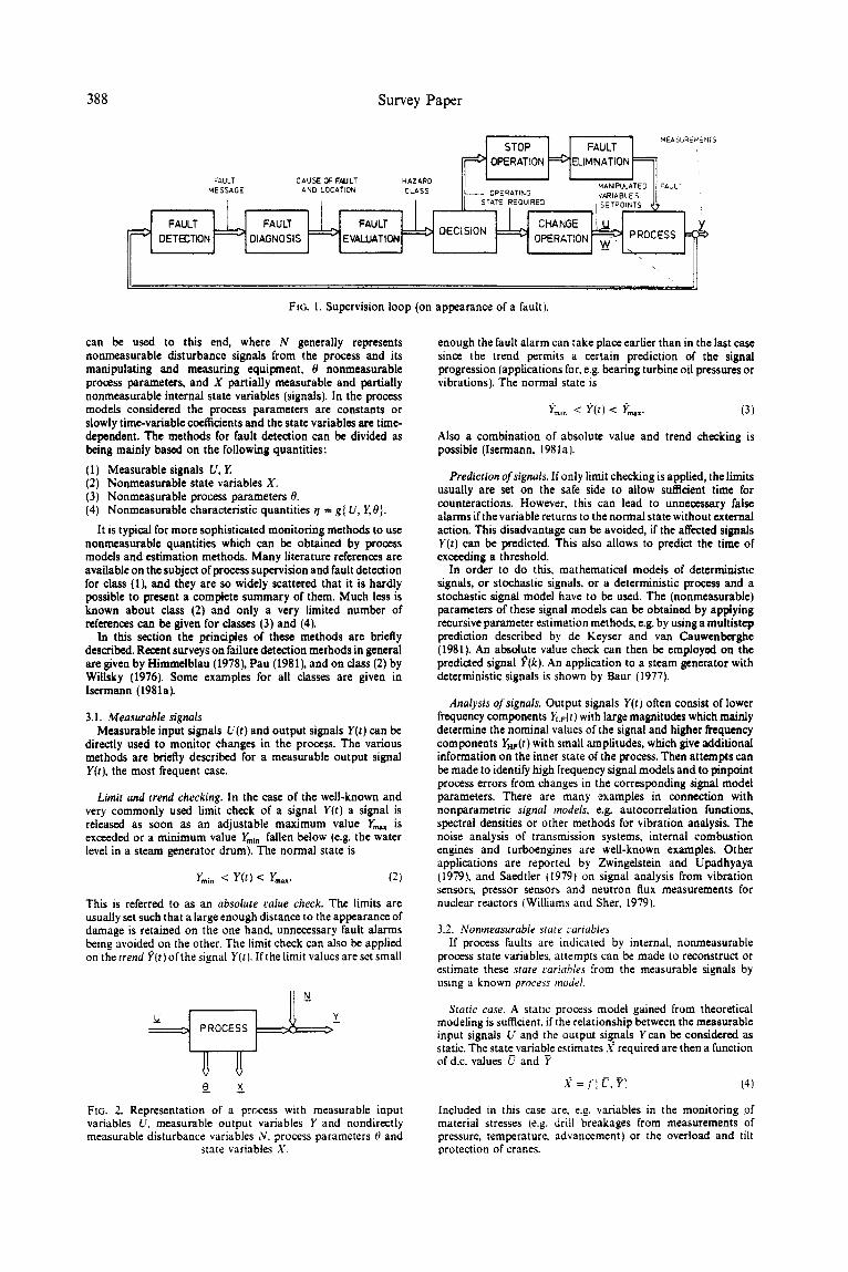
A recent description of the last two statistic methods is given by Willsky (1980). A block diagram of these state variable techniques is shown in Fig. 3.

Of course, these methods require a relatively exact knowledge of the process parameters (A, B. C) and the influencing signals.

3.3. Nonmeasurable process parameters Process model parameters are understood as constants or

time-dependent coefficients in the process which appears in the mathematical description of the relationship between the input and output signals, the process model. A distinction is made between static process models, e.g. in the form of a polynomial equation

Y(U) = flo + fl, U + f12U2 + ... (12)

___....,..PROCESS ) F . . . . . . ,

I ! - ~ [ n l

J 1

i . . . . . j

Y ==~

STATE [ ESTIMATION['-

ESIDUALS I

FAULT DECISION ]

FAULTS

FIG. 3. Fault detection based on state variable estimation.

and dynamic process models which, for processes with lumped parameters, are usually differential equations

y(t) + a~( t ) + a2y(t) + ... + a.y~")(t) = bou(t)

+ bxfi(t) + b2fi'(t) + ... + b.,u(")(t) 113)

in the simplest case lincarized about one operating point. The process model parameters O r = [~ofllB2...] or O r = [a , . . . a . i b l . . . b . ] are mostly more or less intricate relationships of several physical process coefficients, e.g. length, mass, speed, drag coefficient, viscosity, resistances, capacities. Faults which make themselves noticeable in these physical process constants are therefore also expressed in the process model parameters.

If the physical process coefficients which indicate process faults are not directly measurable, an attempt can be made to determine their changes via the changes in the process model parameters O. The following procedure is available:

(a) Establishment of the process equation for the measurable input and output variables

Ytt) = f { U(t),O} 04)

mostly by theoretical modeling. (b) Determination of the relationship between the model

parameters 0~ and the physical process coefficients p j: 0 ---- f(p).

(c) Estimation of the model parameters 01 as a result of measurements of the signals Y(t) and U(t).

(d) Calculation of the process coefficients:

p =f-1(O) (15)

and determination of their changes Apj. (e) Possible process faults can be pinpointed (if need be by

pattern recognition) by the use of a catalogue of faults in which the relationship between process faults and changes in the coefficients Apj has been established.

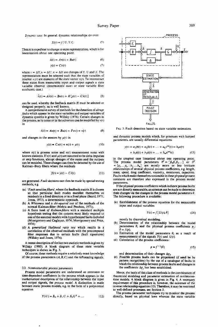
Hence, the basis of this class of methods is the combination of theoretical modeling and parameter estimation of continuous- time models. A block diagram is given in Fig. 4. A necessary requir~acnt of this procedure is, however, the existence of the inverse relationship equation (15). Therefore, it may be restricted to well-defined proce~'s, see Section 5.

The process parameter techniques try to monitor the process directly, based on physical laws whereas the state variable

390 Survey Paper

PROCESS P - l

u , r ~ Jl ) y

IPROCESS~ M OOEU NO

FAULTS

FIG. 4. Fault detection based on parameter estimation and theoretical modeling.

techniques must assume the process parameters as known and try to monitor the signals. Of course, both techniques complement one another.

3.4. Nonmeasurable characteristic quantities The current checking of characteristic quantities can give

important information on the inner state when supervising larger plants or sections.

Examples of characteristic quantities are:

(a) Efficiency (e.g. all types of engines and machines, steam generators, heat exchangers, furnaces, vehicles).

(b) Fuel consumption per production unit or time (e.g. cement burning, milling, drying).

(c) Oil consumption per production unit or time (e.g. internal combustion engines, compressors).

(d) Teol usage per production unit or time (e.g. machine tools). (e) Wear per production unit or time (e.g. tools" motors, grinding

devicesl.

The characteristic quantities must be determined from measurable variables:

= g / u , r~. (16)

Mostly, static relationships are sufficient. Changes in the quantities can point to faults, e.g. contamination, deposits" wear, friction, icing, leaks. To this end, absolute value or trend checks should be carried out on the characteristic quantities.

3.5. A general structure of process fault detection methods Looking at the various tasks of process fault detection

methods which make use of nonmeasurable quantities and therefore are based on process models one recognizes several similarities. Hence, it is straightforward to present these methods in a generalized structure (Fig. 5). Based on the a priori knowledge and experience of the real process we will use:

(i) a model of the normal process; (ii) a model of the obserred process:

(iii) models of the fizulty process.

As the methods rely on the determination of changes in comparison to the normal status, the model of the normal process must be known and tracked with high precision. This also includes the definition of what is "normal', e.g. parameter values including their 'normal' (allowable) tolerances. The normal model can, for

example, be the model obtained just before a fault is alarmed, i.e. the previous model. The models of the faulty process show the effects of the faults on the analysed quantities. These effects are called fault signatures.

Dependent on the faults to be detected one has to use:

(i) state estimation methods; (ii) parameter estimation methods;

(iii) calculation of characteristic quantities.

A comparison of these nonmeasurable quantities x', 0, ~ as part of the observed model with the corresponding quantities of the normal model (i.e. previous model) results in changes

±~, zxO or zx6

or in error signals or residuals, e.g.

= y - C ~ o r e = y - ~P0

if the effect of several estimates on particular signals is considered (h v: see next section). These changes or residuals form comparison quantities and are one basis for the next step, the fault decision. The other basis is the fault signatures which show the effect of faults on these quantities, for example, by:

(i) changes (bias) in definite directions; (ii) changes in opposite directions;

(iii) changes due to a certain pattern; (iv) increase of variances.

Therefore, the changes can be examined with respect to the indication of possible faults. To compare the changes with the fault signatures just binary decisions combined with excecding predetermined thresholds can be made, or more sophisticated methods like correlations of the changes with the failure signatures may be used. This is obviously a field for the application of statistical decision theory and pattern recognition. The result of the fault decision is the fault type and the time of its occurrence.

The next task consists of the fault diagnosis with the goals to determine the fault location, the fault size and the cause of the fault. Again the observed and normal process model may be used to perform this. Based on this information the fault evaluation can start, etc., see Fig. 1.

In the following two examples process fault detection n'~thods are considered which try to monitor changes of process parameters and process state variables. As parameter estimation for continuous-time models is required, suitable methods are considered next.

4. Parameter estimation for continuous-time models Fault detection, based on process parameters which are mostly

not directly measurable, requires on-line parameter estimation methods. As the goal is not only to detect but to diagnose process faults, the process models should express as dose as possible the physical laws which govern the process behaviour. Therefore, the process models have to be developed first by theoretical modeling, that means by stating the balance equations for mass, energy and momentum, the physical-chemical state equations and the phenomenological laws for any irreversible phenomena. The models will then appear in the continuous-time domain, in the form of ordinary or partial differential equations. Their parameters 0~ are ex pressed in dependence on process coefficients pj like storage or resistance quantities, whose changes may tell about process faults. Hence, the parameters 01 of continuous-time models have to be estimated.

Also, in the case of fault detection methods based on state variable techniques, parametric models are required. If their parameters are not known exactly enough, parameter estimation methods also have to be applied.

A comprehensive survey on parameter estimation methods for continuous,time models was given quite recently by Young (1981). For fault detection the single parameters must be estimated very accurately and one of the questions is, for which parameters and for how many parameters (model order) this will be possible in a noisy environment.

Having in mind these requirements, the next sections will briefly discuss some parameter estimation methods for linear,

Survey Paper 391

IN y

PROCESS

MODEL OBSERVED PROCESS

GENERATION OF I - CHANGES - ERROR SIGNALS - RESIDUALS

JJ COMPARISON QUANTITIES

I FAULT ~ FAULT DECISION SIGNATURE

FAULT ~ ~ FAULT TYPE . . . . . TIME

FAULT DIAGNOSIS

FAULT FAULT CAUSE LOCATION SIZE OF FAULT

"4

FIG. 5. Generalized structure of fault detection methods based on process models and nonmeasurable 'quantities.

continuous-time models, based on sampled signals, obtained by a process or microcomputer.

4.1. Least-squares parameter estimation. It is assumed that a stable process with lumped parameters is time-invariant and linearizable so that it can be described by a linear differential equation,

~ ( t ) + a . _ L ~ - l ( t ) + . . . + aly~(t) + aoy°(t)

= b . u ' ( t ) + b = _ l u ' - ~ ( t ) + . . . + blul ( t ) + bou°(t) (17)

where the superscript notations means the time derivative operation, that means yJ(t) = d~y(t)/dt J, and y(t) and u(t) are the deviations

y(t) = Y ( t ) - Yoo; u(t) = U(t) - Uoo. (18)

The measured output y(t) is assumed to be contaminated by a stationary stochastic noise n(t), see Fig. 4,

y(t) = y ,( t ) + n(t). 09)

Substituting for .~(t) in terms of its measurements one obtains

y"(t) = q/T(t)O + eft) (20)

where e(t) is the equation error.

Now measurements of the input and output signals are made and all required derivatives are determined at discrete times t -- kTo, k - - 0 , 1 , 2 , . . . N with To the sampling time. Then N + 1 equations

y~(k) = ~T(k)O + e(k) (21)

result where e(k) can be interpreted as an equation error, resulting in a vector equation

y" = ud0 + e. (22)

The data matrix consists of N + 1 rows of the data vector Or(k). With the cost function

N

V= y. e2(k) --- ere and dV/dO = 0 (23) k=O

the least squares estimate of the parameter vector becomes the well-known nonrecursive estimation equation

0 = [o. /T~ ] - I~JTj~. (24)

However, these parameters are biased for any noise n(t), Therefore, the least-squares method should not be used, if the noise-to-signal ratio is not small.

4.2. Determination o f the time derivatives. The parameter estimation of least-squares requires the time derivatives of the input signal u(t) and the (noisy) output signal y(t) up to the ruth and the (n - ! )th degree, respectively. There are mainly following possibilities to calculate these values from sampled measurements u(k) and y(k).

In the case of numerical differentiation the simplest way is to replace the derivatives by the corresponding (backward) differences. To reduce somewhat the influence of the noise interpolation formulas there is another way. For example, interpolation by splines (third order polynomials) or Newton interpolation can be used. However, the remaining noise influence restricts the application to second and third order processes.

The use of state variable f i l tering according to both the input signal u(t) and the output signal y(t), simultaneously provides the

392 Survey Paper

time derivatives and filters the noise without differentiation (Young, 1981).

Since only the time derivatives of the signals are required there is some freedom in the choice of the filter parameters (Young and Jakeman, 1980).

4.3. Instrumental variables parameter estimation. To overcome the bias problem estimation of the instrumental variable (IV) concept can be used (Young, 1970, 1981 ). Instrumental variables are introduced which are only insignificantly correlated with the noise-free process output y,(t). A suitable way to generate the instrumental variables is to use an auxiliary model of the process which generates the instrumental variables.

This method yields consistent parameter estimates. To start the procedure, the least-squares methods can be used. It is also well suited to be programmed in a recursive form. For further details and improvements s~e Young (1981).

A major advantage of the IV method is that no strong assumptions and knowledge on the noise are required. However, in dosed loop configurations biased estimates are obtained, because the input signal is correlated with the noise.

If on-line real-time parameter estimation is required both the least squares and the instrumental variables method can be written in recursive form (lsermann, 1981b).

4.4. Parameter estimation via discrete-time models. As the parameter estimation methods for discrete-time systems are fairly well developed one can first try to estimate the parameters of the discrete-time model and then to calculate the parameters of the continuous-time model by suitable transformation relation- ships. Mainly, two approaches are used, which are described, e.g. by Sinha and Lastman (1982), Strmrnik and Bremgak (1979) and Hung, Liu and Chou (1980).

However, these methods require extensive computation and are, in part, not straightforward, so that they are, at least in the present status, not feasible for on-line real-time applications.

In conclusion, it can be stated that contrary to discrete-time models the parameter estimation methods for continuous-time models have not obtained the same status. There is still a need for robust parameter estimation methods with less computational effort which provide consistent and efficient parameter estimates under many noise conditions and also in closed loop and for time-variant processes.

5. Fault detection for an electromotor driven centriJugal pump The early detection of process faults is of course especially

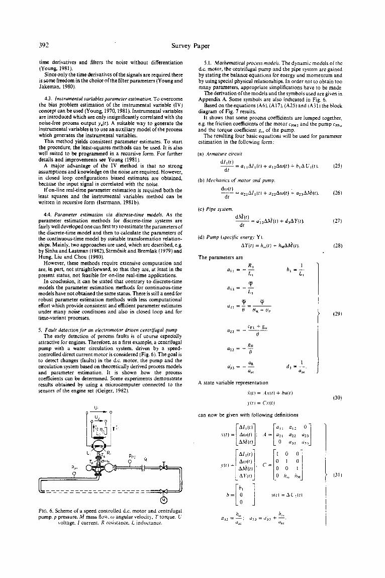
attractive for engines. Therefore, as a first example, a centrifugal pump with a water circulation system, driven by a speed- controlled direct current motor is considered (Fig. 6). The goal is to detect changes (faults) in the d.c. motor, the pump and the circulation system based on theoretically derived process models and parameter estimation. It is shown how the process coefficients can be determined. Some experiments demonstrate results obtained by using a microcomputer connected to the sensors of the engine set IGeiger, 1982).

U,

iJ TiI- P I

Tp / O--td

Pp,

?

PP2 K,I

FIG. 6. Scheme of a speed controlled d.c. motor and centrifugal pump. p pressure, ?v'l mass flo~. c~ angular velocity, T torque. U

~oltage. I current. R resistance. L inductance.

5.1. Mathematical process models. The dynamic models of the d.c. motor, the centrifugal pump and the pipe system are gained by stating the balance equations for energy and momentum and by using special physical relationships. In order not to obtain too many parameters, appropriate simplifications have to be made.

The derivation of the models and the symbols used are given in Appendix A. Some symbols are also indicated in Fig. 6.

Based on the equations (A6), (AI7), (A25) and (A31 } the block diagram of Fig. 7 results.

It shows that some process coefficients are lumped together, e.g. the friction coefficients of the motor CFM1 and the pump Cw~, and the torque coefficient g,~ of the pump.

The resulting four basic equations will be used for parameter estimation in the following form:

{a) Armature circuit

dlz(t) - - = al lAlt( t ) + a12Aco(t) + btA Ul(t).

dt (25)

(b) Mechanics. of motor and pump.

dco(t__~) = a:lAll(r) + a22Aco(t) ~- a23Ah4(t). dt

(26)

(c) Pipe system.

dM(t) = a~3AM(t) + d3AY(t}. (27) dt

(d) Pump (specific energ_ Y).

AY(t) = ho, lt) + hMAAI(t). (28)

The parameters are

Rl a l l = - - -

L t

(p a l 2 ~ - - - -

Ll

T (,/21 -~-

0

we

0 M + 0[,

CF[ + g ~ a22

0

gM a23 = ----

0

(2 R a33 = - - _ _

aae

1

b~ =L-~-z

1 d 3 = - - .

aa¢

(29)

A state variable representation

.~(t) = .4xlt) + buff)

v t l = Cx l t ) (30)

can now be given with following definitions

F AI~(tl i a t t at., x t t t = / A ~ ( t ) ; .4--- a t a , ,

LA, Itt o a;:

r A''"; :l°° 1 • / Ao~(r) 0 1 0 Yltl=lA3,1(t) ; C = 0 0 hLJ

LAYIt)J o h. .

ho, IL~ a 3 2 = - - ; L/33 = a 3 3 +" - - .

~la¢ Ga¢

a23 l ~t33

(31}

Survey Paper 393

+ _ N I l .

!= ARMATURE CIRCUIT - - ~ MECHANICS ---, I D.C.MOTOR ! D.C.MOTOR I I AND PUMP

- - , ,Iq

PIPESYSTEM I

F~G. 7. Block diagram of the linearized d.c. motor-pump-pipe system.

5.2. Process parameter monitoring. The parameters of (25)-(28) can be estimated by bringing them into the form of(21 ) and by applying, for example, the least-squares method. One of the questions then is, how the various process coefficients which are required for fault detection can be calculated. Therefore several cases of operation and measurements are discussed.

(a) D.c. motor and pump, closed valve. In this case 33 (t) = 0 is valid, so that only (25) and (26) are to be used.

(i) Measured signals: A U~, Al l , Aw

Both equations are written due to (21)

y,(t) = C,.~O,

y:tt) = ~,~(t)O= (32)

where

YA/) = d l , ( t l / d t y2 ( t )=dw( t ) /d t

~/~(t) --- [AII(t)Ato(t)A UI(t) ]

O r =[a l l ~= b~]

~br(t) = [Al~(t)Aw(t)]

O r = [~a~ a=].

(33)

Using (29), the following five process coefficients can be calculated based on the five parameter estimates 0~ and 02:

I

b~ ¸

/~1 = - a . £ 1 = - e , l / b ,

= - a l a £ , = - a , , / / ~ l

0 = ~ / ' a , l = - al.//haal

(34)

Hence, all process coefficients which describe the linearized dynamic behaviour can be calculated. However, the friction coefficients of the motor crm and the pump cvu,~ and the moments of inertia 0M and 0p are lumped together so that only their sum can be gained.

If not the dynamic behaviour, but only the static behaviour could be identified, LI and 0 could be not obtained, see (A6) and (A25) for d/dt = O. This shows that by identifying the dynamics more parameters can be estimated and therefore more process coefficients can be monitored.

A disadvantage of the iinearized dynamic relationships is that the coefficients Cruo and Crpo for the adhesive friction do not appear. However, from (A3) and (A10) it follows with the assumption that the friction torque only depends linearly on the speed

Tr~(tl = Cruo + crmto(t)

T~(t) = Crpo + Cvplto(t)

dw(t ) ~ ~ = ~ I ,H) - Cvo - CwW(t)

0

(35)

Cl-lb ~- L'FM O --~ CFp 0

CFI ~--- CFM 1 "at" CFp I .

Then the absolute values w(tt and 11(, ), and not their deviations. are used and the estimation of Cro also becomes possible (Geiger, 1982).

(ii) Measured signals: U I, zxw

It is now assumed that the armature current l~(t) cannot be measured, but only the input U,( t )andtheoutput to(t). Equation (A6) and (A25) then lead to the model

dato(t) d t o ( t ) dt = + ~l---~t + ~totO(t)--- floAU1(t ) (36)

with

R 1 CFI l ] ~' = - E + T ~o = aT-Ic~,Rl + ~ ' )

(37) #o = ---~" ( c r , = cvu~ + cFp~).

L~ '

As there are five unknown process coefficients and only three estimated parameters, the process coefficients cannot be calculated uniquely. Two coefficients have to be known. If 0 and L~ are known, R1,1P and cvl can be determined. This example shows that it is important to measure as many variables as possible. If the static behaviour can be identified, only one parameter

could be estimated. Then two coefficients have to be assumed as known, to determine one coefficient. Hence, also in this case more coefficients are obtained by the use of dynamic models.

If too little or no coefficients can be assumed as known, the single process coefficients cannot be calculated. However, then the changes of the parameter estimates can be monitored. Table 1 shows the sign of these parameter estimates in dependence on the changes (faults) of the process coeffidents. In this case only one pattern is unique, that for Aq ~. Then also the magnitudes of the changes may be taken into account, to detect which of the process coefficients has changed, using their nominal values and sensitivity functions.

(b) D.c. motor, pump and pipe system ( rahe opened). Now all four equations (25)-(28) have to be used.

(i) Measured signals: A U1, Al l , Aco, AY(t), A33(t)

The four equations are now

y~(t) = ~br(t)Oj j --- 1,2,3,4 ( 3 8 )

394 Survey Paper

TABLE 1. PATTERN FOR THE SIGN OF THE PARAMETER CHANGES

At/t A% Afio

+ A R t + + 0 + A~ 0 + + + AL~ - - - + / t 0 - - - + Acvt + + 0

where

yl(t) = dl t ( t ) /d t y2(t) = dto(t)/dt (39)

ya(t) = dAYt(t)/dt y,,(t) = AY(t)

~ r l t ) = [ A l 2 ( t ) Aco(t) AU~(t)]

o r = [ a l a at2 hi]

~,]'(t)= [All(t) Ata(t) A~t(t)]

O r = [azl a ~ a2a] (40)

¢~(t) = JAM(t) AY(t)]

O r = [a~3 d3]

~/( t) = [Aco(t) AM(t)]

or= [h,~ h~]

By using (29) ten process coefficients can be calculated from the ten parameter estimates 0j.

1

/ ~ l = - ' ~ 1 1 £ ~ = - tilt//~l

= -- dt2L~. = - dt2/b t

0 = ~ / d 2 1 = - at21bla2t OF, d- g , m -- ti220 m d22tilI/bld2t (4l)

gM m -- d230 = a23a12/bldZl

d.o = 1/d3

~M}directly available from 0,.

Also in this case all process coefficients are obtainable and can he monitored. In addition to the last ease, cFl and g,~ are lumped together.

The use of dynamic models instead of static models enables one to estimate L~, 0 and a~.

(ii] Some signals not measurable

The problems which arise,, if I d t ) cannot be measured, have been already discussed, see (36). Therefore it will be assumed that at least Uttt), l~(t) and ~o(t) are measured.

Y(t) not measurable, but ~ ( t ) .

Introduction of (28) into (27) leads to

d,~tt) - - = (a'~3 + d3h~)A,(l(t) + d3h~A~o(t). (42)

dt

Hence. as a~3, d 3, h u and h~, are not obtained separately, the process coefficients an, a~¢. h~, h~, and Cr~ cannot be determined

uniquely. However, all remaining six coefficients can still be obtained.

l~t(t) not measurable, but Y(t).

Replacing A~Q(t) in (26) and (27) by use of t28) leads to

= a21AIl(t) - - A~(t) + a23 A Y ( t ) (43) hM

dY(t) , dto(t) d---~- = (a~3 + d3hM)AY(t) + no, T - h~a'33A69(t) (44)

Now d3, hu and a23 are not obtainable separately and therefore the process coefficients an, a,¢, hu, g~ and cvt cannot be determined uniquely, but only the remaining five coefficients.

M(t) and Y(t) not measurable.

Inserting (28) and (27) into (26) yields

d2m(t) din(t) dl l( t) dt 2 = ~z T + 2o + / ~ t T +/~oAlt(t) (45)

with

~ 2 = - (a33 + d3hM - a22)

• 2 = a22(d3hu - a~3) - a23d3h~

f12 = a21

flo = a~3d3hMa2t.

(46)

Based on (25), three process coefficients can be estimated: L t, R) and ~/. As/J1 enables us to estimate 0. three parameter estimates remain to determine six coefficients, which is not possible uniquely. Therefore three process coefficients are assumed to be known. Hence, in this case. only four process coefficients can be calculated uniquely.

If the sensors do have dynamics which cannot he neglected in comparison to the process, they must also be included in the process model.

5.3. Experimental results. Experiments were made with a centrifugal pump driven by a speed controlled d.c. motor. The technical data are

(a) D.c. motor: maximum power P , , . = 4kW maximum rotation speed Nm.~ = 3000revmin-1.

(b) Centrifugal pump, one stage: maximum total head Hm~ - 39 m for Nm,~ - 3000 rev min - i.

(c) Pipe system: length: L ~ 10m diameter: dl = 50 ram.

The d.c. motor is controlled by an a.c./d.c, converter with cascade control of the speed and the armature current as auxiliary control variable. The manipulated variable is the armature current Ut. A microcomputer DEC-LSI 11/23 was connected on.line to the process. For the experiments the reference value W(t) of the speed control has been changed stepwis¢ with a magnitude of 2 ~ /o f N,,~, i.e. 60 rev rain- t every 60s. The measured signals were sampled with sampling time To -- 2 ms over a period of 2 s, so that 1000 samplings were obtained.

These measurements were stored in the core-memory. After 2 s measurements the parameters were estimated off-line, using the recursive least-squares method with state variable filters for the determination of the time derivatives. The available computation time for the parameters was 58s. Hence, one set of parameter estimates was obtained every minute. As the noise is negligibly small, the parameter estimates can be assumed to be unbiased.

The first experiments were performed with closed valve. As

Survey Paper 395

described before (d.c. motor and pump, closed valve) then two equations can he applied for the parameter estimation. In order to also obtain the adhesive friction coefficient, (35) has been used

0 dco(t) = ip l , (t) - Cro - cwoJ(t) dt

together with (A1) for the armature circuit

dll(t) L~

dt = UI(t)- Rill(t) - ~ c o ( Z ) .

Therefore the deviations of the signals have to be replaced in (33) by their absolute values. The process coefficients are obtained by (34) with ~vo = - '~,30 in addition.

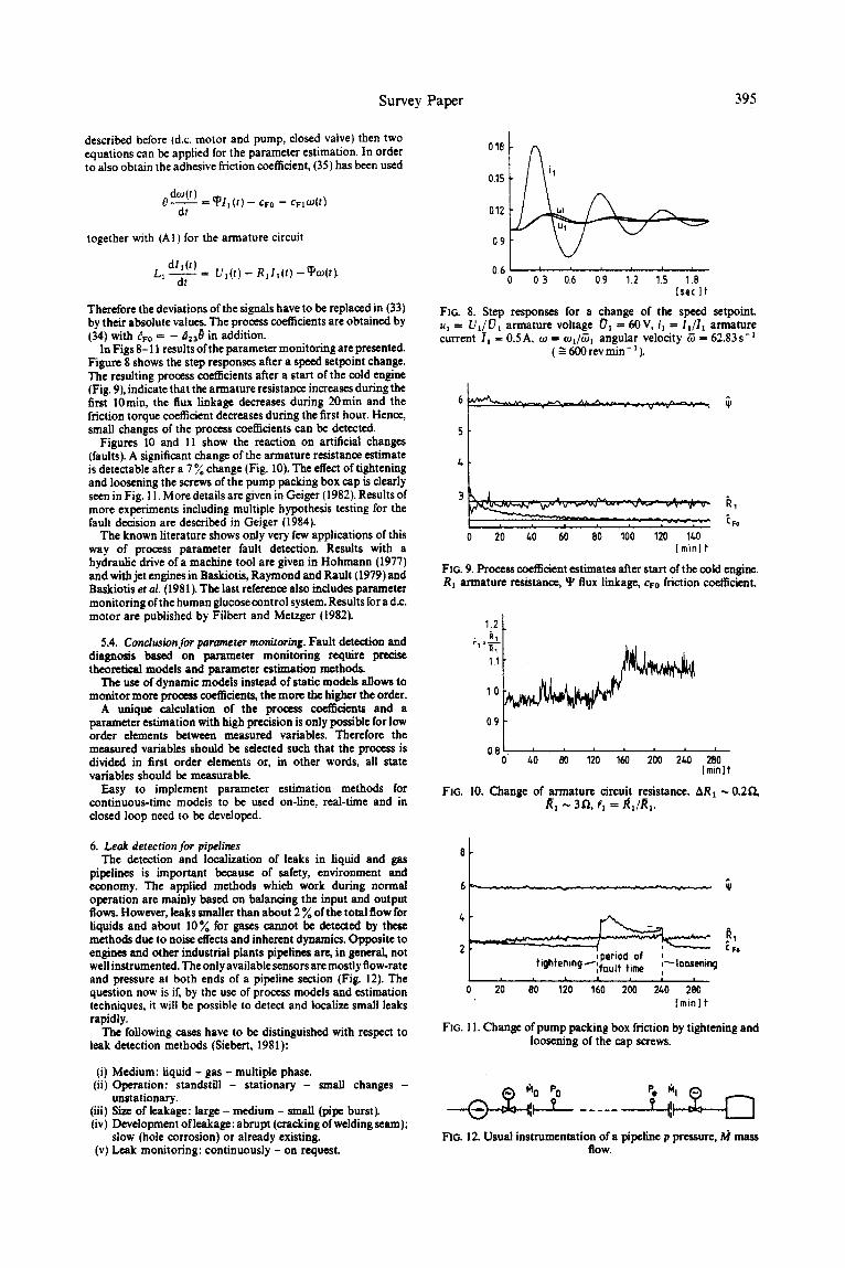
In Figs 8-11 results of the parameter monitoring are presented. Figure 8 shows the step responses after a speed setpoint change. The resulting process coefficients after a start of the cold engine (Fig. 9), indicate that the armature resistance increases during the first 10min, the flux linkage decreases during 20rain and the friction torque coefficient decreases during the first hour. Hence, small changes of the process coefficients can be detected.

Figures 10 and 11 show the reaction on artificial changes (faults). A significant change of the armature resistance estimate is detectable after a 7 % change (Fig. 10). The effect of tightening and loosening the screws of the pump packing box cap is dearly seen in Fig. 11. More details are given in Geiger (1982). Results of more experiments including multiple hypothesis testing for the fault decision are described in Geiger (1984).

The known literature shows only very few applications of this way of process parameter fault detection. Results with a hydraulic drive of a machine tool are given in Hohmann (1977) and with jet engines in Baskiotis, Raymond and Rault (1979) and Baskiotis et al. (1981). The last reference also includes parameter monitoring of the human glucose control system. Results for a d.c. motor are published by Filbert and Metzger (1982).

5.4. Conclusion for parameter monitoring. Fault detection and diagnosis based on parameter monitoring require precise theoretical models and parameter estimation methods.

The use of dynamic models instead of static models allows to monitor more process coefficients, the more the higher the order.

A unique calculation of the process coefficients and a parameter estimation with high precision is only possible for low order elements between measured variables. Therefore the measured variables should be selected such that the process is divided in first order elements or, in other words, all state variables should be measurable.

Easy to implement parameter estimation methods for continuous-time models to be used on-line, real-time and in closed loop need to be developed.

0.15 iI

0.12 ~1

0.9

0.6 ' ' ' ' 1.'5 t 0 3 06 09 1.2 1.8

[sec ]t

Fla. 8. Step responses for a change of the speed setpoint. ul ffi U1 /01 armature voltage 01 = 60V, il = f i l l s armature current 11 = 0.5A, co = (ol/G 1 angular velocity ~ = 62.83s -=

( ~ 600 rev min- ~).

. . . . . v - - v

5

3 _l . . . . . . . . . . . . . . ~, _2r2 5 V .

, - - ~ - - CFo t J ! , ,

0 20 /~0 60 80 100 120 1/.0 [ rain] t

FIG. 9. Process coefficient estimates after start of the cold engine. RI armature resistance, ~P flux linkage, Cvo friction coefficient.

1.2

r I = ~- -~

11

10

09

0 .8 ' ' ' ' 2"00 ' ' ~,0 80 120 160 2~0 280

[minlt

FIG. 10. Change of armature circuit resistance. ARs ,,, 0.2fl, /~1 ~ 3fl, ~1 = ~1//I1.

6. Leak detection for pipelines The detection and localization of leaks in liquid and gas

pipelines is important because of safety, environment and economy. The applied methods which work during normal operation are mainly based on balancing the input and output flows. However, leaks smaller than about 2 % of the total flow for liquids and about 10% for gases cannot be detected by these methods due to noise effects and inherent dynamics. Opposite to engines and other industrial plants pipefines are, in general, not well instrumented. The only available sensors are mostly flow-rate and pressure at both ends of a pipeline section (Fig. 12). The question now is if, by the use of process models and estimation techniques, it will be possible to detect and localize small leaks rapidly.

The following cases have to be distinguished with respect to leak detection methods (Siebert, 1981):

(i) Medium: liquid - gas - multiple phase. (ii) Operation: standstill - stationary - small changes -

unstationary. (iii) Size of leakage: large -med ium - small (pipe burst). (iv) Development of leakage: abrupt (cracking of welding seam);

slow (hole corrosion) or already existing. (v) Leak monitoring: continuously - on request.

6

2

t t I

0 20 8 0 120

. . ~ period of hghtening" ' , f~ul t time ,~loosening

160 2O0 2hO 280 [m in ] f

C Fo

FZG. 1 I. Change of pump packing box friction by tightening and loosening of the cap screws.

FIG. 12. Usual instrumentation of a pipeline p pressure, ~ mass flow.

396 Survey Paper

In the following, methods for leak detection will be discussed for liquids and gases, stationary operation with small changes of the variables, small leaks which appear abrupt, and continuous monitoring.

6.1. Mathematical process models. The dynamic models of a pipeline and the symbols used are described in Appendix B. Based on the mass and momentum balance equations, the quadratic friction law, the isothermic gas state equation and various simplifying assumptions a nonlinear hyperbolic partial differential equation system is obtained, (B9). After dividing the pipeline in 1/2 sections and discretization of the differential equations, a set of ordinary differential equations results which forms a nonlinear state space model, see (B15).

For small changes and the flow ~ in the positive z-direction, the momentum balance equation of (BI2) can be linearized

0Mj Ot = g2(AP~+I - Ap~_l) + 2g;(~_ I)AMj (47)

where all coelficients are taken for the steady-state values pj and M'j. Further on the linearized valve equations are introduced in the form

Ape = C',oAldo + Ap,o )

Ap,, ffi c'...A34",. + Ap,~. ? (49)

Then a linear state representation

Yc(t) = Ax( t ) + Bu(t) (49)

y(t) = Cx{t)

results, with

xr( t ) = [AMoAM2... AMI I Ap1Ap~. . . Apl - l ]

ur [APi*AP'~ ] I (50)

However, for most of the gas pipelines the nonlinear (B 15) must be used. It is because of their big storage capacities and the time- dependent consumption that they rarely come to a steady state.

6.2. Methods for leak detection. It is assumed that a small leak flow d2~ t occurs at section j = ¢. The effect of the leak can be modeled by introducing this leak flow into the mass balance of this section, see (BI8), leading to (B20). This changes the linearized state equation (49) to

.~(t) = Ax(t ) + Lv(t) + Buff) (51)

with the leak flow vector

vr ( t )= [0 0 . . . l ~ L ~ . . . 0 i 0 . . . 0 ] (52)

and the leak influence matrix

i0 0 01 L = / ° ... 0 0 ... Ol (53) ..... 6 .....

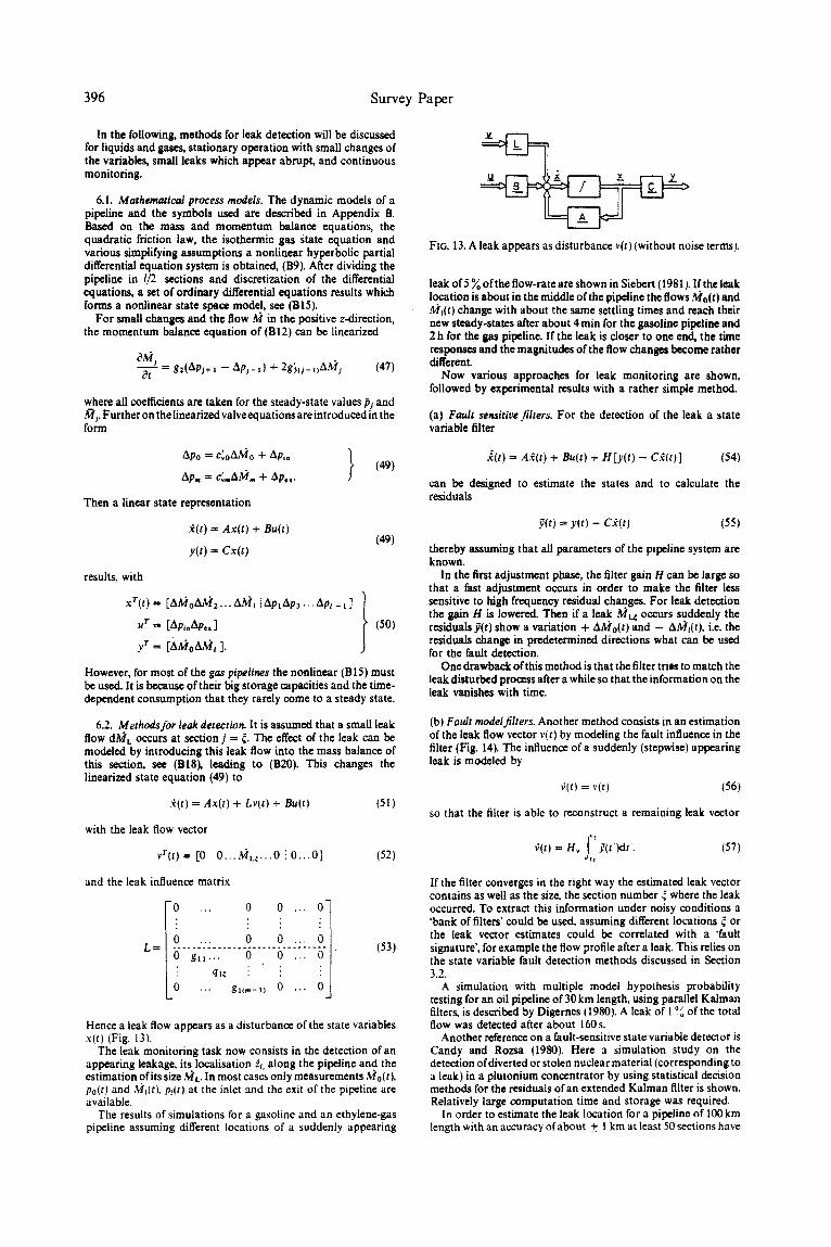
: qt~ : 0 0 Lo ... , , , . - , , . . . J Hence a leak flow appears as a disturbance of the state variables x(t) (Fig. 13).

The leak monitoring task now consists in the detection of an appearing leakage, its localisation ~t along the pipeline and the estimation of its size ,'~'L. In most cases only measurements/~0(t k po(t) and Mr(t), p~(t) at the inlet and the exit of the pipeline are available.

The results of simulations for a gasoline and an ethylene-gas pipeline assuming different locations of a suddenly appearing

Z

FIG. 13. A leak appears as disturbance v(t) (without noise terms).

leak of 5 ~ oftbe flow-rate are shown in Siebert (1981). If the leak location is about in the middle of the pipeline the flows .~o(t) and Mdt) change with about the same settling times and reach their new steady-states after about 4min for the gasoline pipeline and 2 h for the gas pipeline. If the leak is closer to one end, the time responses and the magnitudes of the flow changes become rather different.

Now various approaches for leak monitoring are shown, followed by experimental results with a rather simple method.

(a) Fault sensitive filters. For the detection of the leak a state variable filter

S;(t) = A.~(t) + Bu(t) + H[y( t ) - C.~.(t) ] (54)

can be designed to estimate the states and to calculate the residuals

.~(t) = y(t) - C~(t) 05)

thereby assuming that all parameters of the pipeline system are known.

In the first adjustment phase, the filter gain H can be large so that a fast adjustment occurs in order to make the filter less sensitive to high frequency residual changes. For leak detection the gain H is lowered. Then if a leak MLg occurs suddenly the residuals .P(t) show a variation + AMo(t) and - A~dt), i.e. the residuals change in predetermined directions what can be used for the fault detection.

One drawback of this method is that the filter tries to match the leak disturbed process after a while so that the information on the leak vanishes with time.

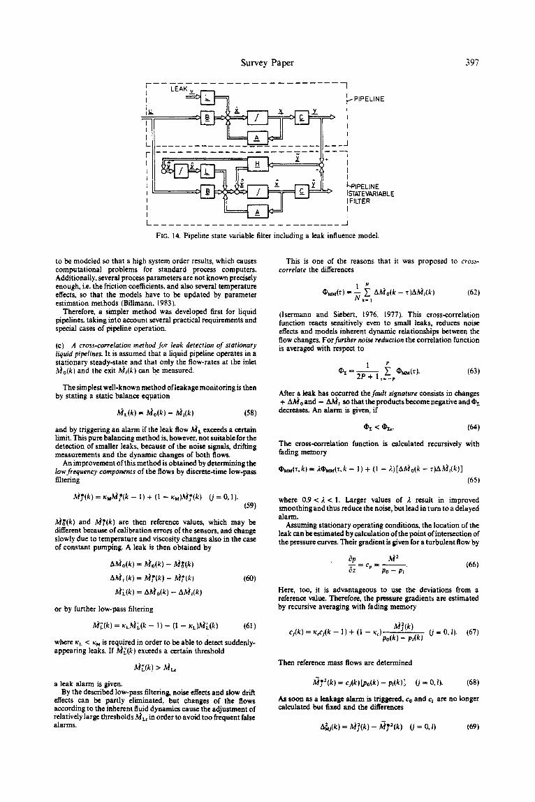
(b) Fault model filters. Another method consists in an estimation of the leak flow vector v(t) by modeling the fault influence in the filter (Fig. 14). The influence of a suddenly (stepwise) appearing leak is modeled by

¢ ( t ) = v ( t ) (56)

so that the filter is able to reconstruct a remaining leak vector

f IL 37(t')dt'. ¢(t) = H, (57)

If the filter converges in the right way the estimated leak vector contains as well as the size, the section number ~ where the leak occurred. To extract this information under noisy conditions a 'bank of filters" could be used, assuming different locations ~ or the leak vector estimates could be correlated with a 'fault signature', for example the flow profile after a leak. This relies on the state variable fault detection methods discussed in Section 3.2.

A simulation with multiple model hypothesis probability testing for an oil pipeline of 30 km length, using parallel Kalman filters, is described by Digernes (1980). A leak of 1% of the total flow was detected after about 160 s.

Another reference on a fault-sensitive state variable detector is Candy and Rozsa {1980). Here a simulation study on the detection of diverted or stolen nuclear material (corresponding to a leak) in a plutonium concentrator by using statistical decision methods for the residuals of an extended Kalman filter is shown. Relatively large computation time and storage was required.

In order to estimate the leak location for a pipeline of I00 km length with an accuracy of about + 1 km at least 50 sections have

S u r v e y P a p e r 397

T i l

[

L r-

L E A K ~ ==={> ,.-.PIPELINE

t',-PIPELIN E ISTATEVARIABL E I FILTER I I

._1 FIG. 14. Pipeline state variable filter including a leak influence model.

to be modeled so that a high system order results, which causes computational problems for standard process computers. Additionally, several process parameters are not known precisely enough, i.e. the friction coefficients, and also several temperature effects, so that the models have to be updated by parameter estimation methods (Billmann, 1983 ).

Therefore, a simpler method was developed first for liquid pipelines, taking into account several practical requirements and special cases of pipeline operation.

(c) A cross-correlation method .for leak detection o f stationary liquid pipelines. It is assumed that a liquid pipeline operates in a stationary steady-state and that only the flow-rates at the inlet ,~lo(k) and the exit b~l(k) can be measured.

The simplest well-known method of leakage monitoring is then by stating a static balance equation

Mr(k) --- A'J'o(k) -- A,l,(k) (58)

and by triggering an alarm if the leak flow ML e X ~ d S a certain limit. This pure balancing method is, however, not suitable for the detection of smaller leaks, because of the noise signals, drifting measurements and the dynamic changes of both flows.

An improvement of this method is obtained by determining the low frequency components of the flows by discrete-time low-pass filtering

M~'(k) = rM~*(k - I) + (l -- rM)~*(k ) (j = O, 1). (59)

bl~'(k) and MT'(k) are then reference values, which may be different because of calibration errors of the sensors, and change slowly due to temperature and viscosity changes also in the case of constant pumping. A leak is then obtained by

AA4o(k) = A,lo(k ) - J~,l~(k)

a Y t , (k) = M ? ( k ) - M*(k) (6O)

J~J'~.(k) = aA'J*o(k ) - aA,l~(k)

or by further low-pass filtering

~3£(k) = KLML(k -- 1) -- (I -- rL)A'l~.(k) (61)

where rL < ru is required in order to be able to detect suddenly- appearing leaks. If M~(k) exceeds a certain threshold

~ ( k ) > ~

a leak alarm is given. By the described low-pass filtering, noise effects and slow drift

effects can be partly eliminated, but changes of the flows according to the inherent fluid dynamics cause the adjustment of i-elatively large thresholds ML~ in order to avoid too frequent false alarms.

This is one of the reasons that it was proposed to cross- correlate the differences

t O~M(T) = - - ~ AA'/o(k - "c)AMl(k) (62)

Nk=l

(lsermann and Siebert, 1976, 1977). This cross-correlation function reacts sensitively even to small leaks, reduces noise effects and models inherent dynamic relationships between the flow changes. For fur ther noise reduction the correlation function is averaged with respect to

1 e 1 ~ (1)MM(~)" (63) Oz = 2P + = ,= _~,

After a leak has occurred the faul t signature consists in changes + A ~ o a n d - A3dt so that the products become negative and Oz decreases. An alarm is given, if

~, < ~,. (64)

The cross-correlation function is calculated recursively with fading memory

¢PMu(T,k) = 2@uM(z,k -- 1) + (1 -- 2)[AA4o(k - ~)AJ~t(k)]

(65)

where 0.9 < 2 < 1. Larger values of 2 result in improved smoothing and thus reduce the noise, but lead in turn to a delayed alarm.

Assuming stationary operating conditions, the location of the leak can be estimated by calculation of the point of intersection of the pressure curves. Their gradient is given for a turbulent flow by

~p ~3 ~ ~z cp = . (66)

Po - Pa

Here, too, it is advantageous to use the deviations from a reference value. Therefore, the pressure gradients are estimated by recursive averaging with fading memory

, .~/](k) cj(k) = rcc.~(k - 1) + (1 - r d p o ( k ~ _ p : ( k ) (j = O, I). (67)

Then reference mass flows are determined

4 , , j (k) ---- cj(k)~po(k) - p~(k)] (j = 0,1). (68)

As soon as a leakage alarm is triggered, Co and c t are no longer calculated but fixed and the differences

A~j(k) -- lVlf(k) - M~2(k) (j = 0,1) (69)

398 Survey Paper

are determined and summed up. Assuming small leaks the leak location is given by

2r = L (l ZAM°tk)l - ~ / ( 7 0 )

see Siebert and Isermann (1977). In a similar way the leak flow is estimated.

6.3. Experimental results with pipelines. Figure 15 shows the course of the pipeline considering the height above sea level as well as the location of pumps. The two main pumps are driven by two 400kW asynchronous machines, which may be operated individually or together. At full power about 330m3h -~ are delivered at an initial pressure of 69 bar. This pressure is measured after the pumps, but before the entrance valve.

The line has a diameter of 273 mm and a wall thickness of 8 ram. Intermediate depots are located at 21.1, 27.3, 35.8, 43.9 and 46.7 km.

The volume flows are measured by means of measuring orifices and Barton cells, pressures with Barton cells (accuracy about 0.1 ~). The volume flow V (l) at the end oftbe line is transmitted by a telemetric device, i.e. deviations from the operating point- - about 1/10 of the total measuring range (0-400m 3 h - t} - -a re encoded into an 8-bit-word. This corresponds to a resolution of 0.16m3h - t or 0.05~ with respect to 330m3h -t .

Since the pressure at the end of the line was almost constantly equal to atmospheric pressure, recording and processing of the measurement variable p (l) was dispensed with. Thus only both volumetric flows F(0) and V (l), as well as the pressure at the beginning of the pipeline, were used for leakage monitoring. For further details on the pipeline and the equipment see Siebert and Klaiber (1980).

An INTEL MDS 800 microcomputer development system was used to carry out the on-line experiments with the pipeline described above. An 8-bit microcomputer with the 8080 A central processor was used. The system is extended to 48 k of RAM.

An extensive program package--16kbytes of program memory--for leakage monitoring was implemented on the microcomputer system in the ASM 80 assembler language.

A series of experiments for leakage detection were carried out on the pipeline described above, where leaks could be generated artificially at the branches to the intermediate depots.

The following values were assumed for the constants:

xc = 0.9975

,~. = 0.99

Or~= -0 .5

P = 20.

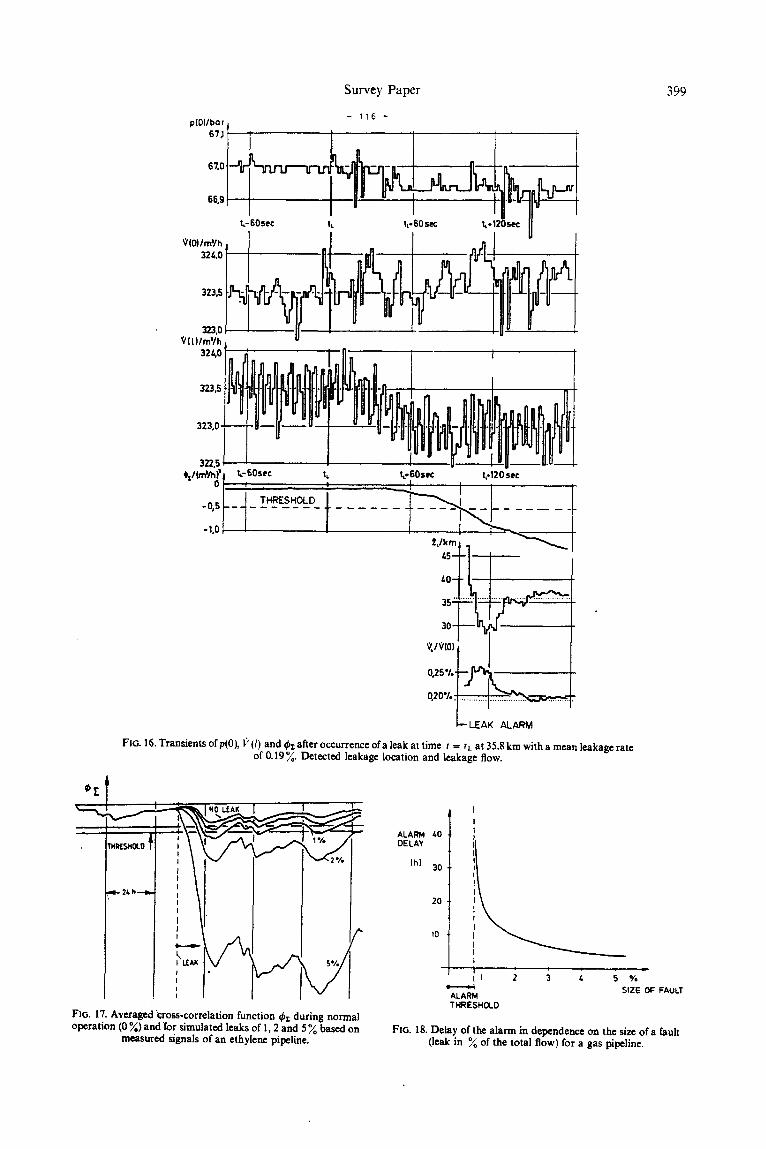
Figure 16 shows one of the experiments carried out. The values of the signals p(0), V(0) and V (I) collected by the microcomputer were recorded, below them the sam of cross-correlation functions Oz for the indication of a leakage is shown. The leak was generated at t = t L. The leakage location and leakage flow calculation after detection of the leak is also shown.

In the experiment shown--leakage location at 35.8 km and mean leakage rate of 0.19% which is about 0.21sec-~--the trigger level was exceeded 98 s after occurrence oftbe leak and the alarm was triggered. The leak location was estimated with an

21.1

h/m 6~_I~---I-"I-.,~.I ) I. l,.A"~J~A1!t , ) I . ,'~ ~ ' ~ ~ - r - ' W ~ - t x - . A ' - - ' r - - - r . /

~ , , I t - i - [ I I ~" I I " • . I I I . . I z/km

2 ~ ~ . a t,3.g ~ y

Ft6. 15. Schematic diagram of the pipeline with topographic vrofile.

error ofabout + 0.7°,; or + 500m at time 90s after the alarm. Since the characteristic variable ~z in all cases significantly

exceeded its standard deviation during regular operation without a leak, it may be assumed that even smaller leaks than those in the experiments carried out can be detected and localized.

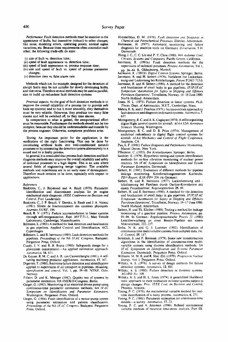
The described cross-correlation method which is well suited for liquid pipelines, was modified for the use of gas pipelines by taking into account the quadratic pressure profile and dynamic models of the pressures and flows (Siebert and Isermann, 1980; Siebert, 1981). Signals of an ethylene pipeline (L= 150km; d~ = 260mm; M = 17th -~) have been measured to verify the dynamic models. Simulation of leaks with these models show (Fig. 17) that the modified cross-correlation method is able to detect leaks of about 2°0 after about 10h and 5% after 3.5h. These results allow to show a typical relationship for fault detection methods between the alarm delay time and the size of the alarm under noisy conditions (Fig. 18). The methods on leak detection are presently further developed (Billmann, 1983; Billmann and lsermann. 1984).

6.4. Conclusions Jor leak detection. Leak detection methods require a precise knowledge of the normal state (precise normal model, or precise reference values).

The use of dynamic models instead of static models enables detection of smaller leaks.

If no precise parametric model from theoretical modeling is known or the computational effort becomes too large, nonparametric models may also be used (cross-correlation method instead of state-model methods).

The leak detection method has to be insensitive to process noise but sensitive to the appearance of a leak. Thus the normal model should only follow low frequency signal components, whereas the leak signature components should be detected in the high-frequency range. The methods are then better suited to detect abrupt leaks than slowly developing leaks.

The influence of drift effects oftbe sensors and the pipeline are to be suppressed by special methods.

Due to the remaining noise effects there is approximately a hyperbolic relationship between the alarm delay and the size of the leak.

Many of these statements hold quite generally for fault detection methods.

7. Concluding remarks An attempt has been made, based on the present knowledge

and experience, to review some fault detection methods. Emphasis has been given on methods for monitoring unmeasurable quantities like process parameters and process state variables. Fault detection methods for these classes make use of process models, parameter and state estimation methods anti statistical decision methods. In designing fault detection methods one should take into account the following aspects.

Process models. In many cases rather accurate process models are required. Hence, as well as theoretical process modeling continuous-time process parameter estimation plays a basic role. The discussed fault detection methods are therefore easier to apply for well-defined processes, like electrical and mechanical processes than for others, such as thermal and chemical processes. Since the methods are based on deviations to a normal process, it is important to define the normal process and to track its normal changes by estimation methods. For small changes of the variables linearized models may be sufficient. In general, however, nonlinear models have to be applied. The use of dynamic instead of static models yields more information and allows detection of more and/or smaller faults.

Parameter and state estimation. If the parameters and states are required with high precision, as for parameter monitoring and fault model filtering, the application is restricted to rather low order model elements. This means that many signals should be measurable for higher order processes.

Faults. Faults may either be already existing or appear at an unknown time, expected or unexpected. Their speed of appearance can be very different, from very large (abrupt faults) to very slowly (drifting faultsL

Survey Paper 399

- 316 - p ( 0 ) / b o r

L T i 6tO . . . .

66,9 ~ ~

t,- 60sec tL It* 60 sec t.° 120sec 9(O)l~h

~'(l.)/rnVh

3z3~4~ 323.0

322.5 Oz/(mm/ho)' l ,$Osec tL tL*EOsec t,*120 sec /

.0,s)_ '~s"°L° t _ -1,o I

~0

35 ......... '"

30

V, IV(O) I

_ °,0'.-L-:E:I.-. FIG. 16. Transients of p(0), P (I) and 0z after occurrence of a leak at time t -- tt at 35.8 km with a mean leakage rate

of 0.19 %. Detected leakage location and leakage flow.

~ E

'HRESHOED I

i I , - 24 h.--B,

NO LEAK I

F]o. 17. Averaged 'cross-correlation function ~z during normal operation (0 %) and'for dmulatcd leaks of I, 2 and 5 % based on

measured signals of an ethylene pipeline.

ALARM 40 DELAY

[h] 30

20

~0

i i i i l t -

1 2 3 4 5 % -ALA~I~_., S IZE OF FAULT

T H R E S H O L D

FIG. 18. Delay of t l~ alarm in dependence on the s i~ of a fault (leak in % of the total flow) for a gas pipeline.

400 Survey Paper

Performance. Fault detection methods must be sensitive to the appearance of faults, but insensitive (robust) to other changes, like noise, modeling errors, ol~rating points, normal signal variations, etc. Because these requirements often contradict each other, the following trade-offs do exist:

(i) size of fault vs. detection time; (ii) speed of fault appearance vs. detection time;

(iii) speed of fault appearance vs. proecss r~ponse time; (iv) size and speed of fault vs. speed of process parameter

changes; (v) detection time vs. false alarm rate.

Methods which are, for example, designed for the detection of abrupt faults may be not suitable for slowly developing faults, and vice versa. Therefore several methods may be nscd in parallel, also to build up redundant fault detection systems.

Practical aspects. As the goal of fault detection methods is to improve the overall reliability of a process (or to provide safe back-up systems) and to run it more smoothly, they themselves must be very reliable. Otherwise, they produ~ too many false alarms and will be switched off, or they miss alarms.

In comparison to what is gained, the computational effort must be reasonable. Furthermore the methods should not bc too complex, because they should be understandable and tunable by the process engineer. Otherwise, acceptano," problems arise,

Testing. An important point for the application is the verification of the right functioning. This can be done by introducing artificial faults into well-conditioned (sound) processes or by connecting the detection system alternatively to a sound and to a faulty process.

In general, it is concluded that proer~s fault deteetion and fault diagnosis methods may improve the overall reliability and safety of technical processes to a high degree. This is an area where several fields of engineering merge together. The available methods and experiences are in an early state of development. Therefore much remains to be done, especially with respect to applications.

References Baskiotis, C., J. Raymond and A. Rault (t979). Parameter

identification and discriminant analysis for jet engine mechanical state diagnosis. IEEE Conference on Decision and Control, Fort Lauderdale.

Baskiotis. C., J. P. Brault, Y. Derekx, A. Rault and J. A. Videau (1981). S~aret6 de fonctionnement des systrmes physiques. Journdes SURF, 196.

Beard, R. V. (1971). Failure accommodation in linear systems through self-reorganization. Rept. MVT-71-1, Man Vehicle Laboratory, Cambridge, Massachusetts.

Billmann, L. 11983). A method for leak detection and localization in gas pipelines. Applied Control and Identification, ACI, Copenhagen.

Billmann, L. and R. Isermann (1984). Leak detection methods for pipelines. Proceedings of the 9th IFAC Congress, Budapest. Pergamon Press, Oxford.

Candy, J. V. and R. B. Rozsa (1980). Safeguards design for a plutonium concentrator--An applied estimation approach. Automatica, 16, 615.

De Keyser, R. M. C. and A. R. van Cauwenberghe (1981). A self- tuning multistep predictor application. Automatica, 17, 167.

Digernes. T. 11980). Real-time failure detection and identification applied to supervision of oil transport in pipelines. Modeling, identification and control, Vol. 1, pp. 39-49. NTNF, Oslo, Norway.

Filbert. D. and K. Metzger (1982). Quality test of systems by parameter estimation. 9th IMEKO-Congress, Berlin.

Geiger. G. (1982). Monitoring of an electrical driven pump using continuous-time parameter estimation methods. 6th IFAC Symposium on Identification and Parameter Estimation, Washington. Pergamon Press, Oxford.

Geiger, G. {1984). Fault identification of a motor-pump system using parameter estimation and pattern classification. Proceedings of the 9th IFAC Congress, Budapest. Pergamon Press, Oxford.

Himmelblau, D. M. 11978). Fault Detection and Diagnosis in Chemical and Petrochemical Processes. Elsevier, Amsterdam.

Hohmann, H. (1977). Automatic monitoring and failure diagnosis for machine tools (in German). Dissertation, T.H. Darmstadt.

Hung, J. C., C. C. Liu and P. Y. Chou (19801. 14th Asilomar Con/~ Circuits, Systems and Computers, Pacific Grove, California.

lsermann, R. (1981a). Fault detection methods for the supervision of technical processes. Process Automation, Vol 1, pp. 36-44. R. Oldenbourg, Munich.

Isermann. R. I 1981 b). Digital Control Systems. Springer, Berlin. Isermann, R. and H. Siebert ~1976). Verfahren zur Leckerken-

nung und Leckortung bei Rohrleitungen. Patent P 2603 715.0. Isermann, R. and H. Siebert (1980). A method for the detection

and localisation of small leaks in gas pipelines. IFIP/IFAC Symposium "Automation for Safety in Shipping and Offshore Petroleum Operations', Trondheim, Norway, 16-18 June 1980. North Holland, Amsterdam.

Jones, H. L. (1973). Failure detection in linear systems. Ph.D. Thesis, Dept. of Aeronautics, M.I.T., Cambridge, Mass.

Mehra, R. K. and J. Peschon ( 1971 ). An innovations approach to fault detection and diagnosis in dynamic systems. ,4 utomatica. 7, 637.

Montgomery, R. C. and A. K. Caglayan (1974), A selfreorganizing digital flight control system for aircraft. AIAA 12th Aerospace Sciences Meeting, Washington.

Montgomery, R. C. and D. B. Price (1974). Management of analytical redundancy in digital flight control systems for aircraft. AIAA Mechanics and Control of Flight Conference, Anaheim, CA.

Pau, L. F. (1981). Failure Diagnosis and PerJbrmance Monitoring. Marcel Derrer, New York.

Pfleiderer, C. (1955l. Die Kreiselpumpen. Springer. Berlin. Saedtler, E. (1979). Hypothesis testing and system identification

methods for on-line vibration monitoring of nuclear power reactors. 5th [FAC Symposium on Identification and System Parameter Estimation, Darmstadt.

Siebert, H. (1981). Evaluation of different methods for pipeline leakage monitoring. Kernforschungszentrum Karlsruhe. PDV-Report, KfK-PDV 206 (in German).

Siebert, H. and R. Isermann {1977). Leckerkennung und - lokalisierung bei Pipelines durch On-line-Korrelation mit einem ProzeBrechner, Regelungstechnik 25. 69.

Siebert, H. and R. Isermann (1980). A method for the detection and localization of small leaks in gas pipelines. IFIP/IFAC Symposium "Automation Jor Safety in Shipping and Offshore Petroleum Operations', Trondheim, Norway, 16-17 June 1980. North Holland, Amsterdam.

Siebert, H. and Th. Klaiber (1980). Testing a method for leakage monitoring of a gasoline pipeline. Process Automation, pp. 91-96. In German: Regelungstechnische Praxis 22 11980) Lecktiberwachung an einer Benzin-Pipeline mit einem Mikrorechner, 232-237.

Sinha, N. K. and G. J. Lastman (1982). Identification of continuous time multivariable systems from sampled data. Int. J. Control, 35, 117.

Strmrnik, S. and F. Bremsak 11979). Some new transformation algorithms in the identification of continuous-time multi- variable systems using discrete identification methods. 5th IFAC Symposium on ldent!tication and Systems Parameter Estimation. Darmstadt. Pergamon Press, Oxford.

Williams, M. M. R. and R. Sher lEd.) {1979). Progress in Nuclear Energy, Vol. I. Pergamon Press, Oxford.

Willsky. A. S. (1976). A survey of design methods for failure detection systems. Automatica, 12, 601.

Willsky, A. S. 11980). Failure detection in dynamic systems. AGARD No. 109.

Willsky, A. S. and H. L. Jones (1974). A generalized likelihood ratio approach to state estimation in linear systems subject to abrupt changes. Prec. IEEE Con]~ on Decision and Control, Phoenix, Arizona.

Young, P. C. (1970). An instrumental variable method for real- time identification of a noisy process. Automatica, 6, 271.

Young. P. C. (1981). Parameter estimation for continuous-time models--a survey. Automatica, 17, 23.

Young, P. C. and A. Jakeman {1980). Refined instrumental variable methods of recursive time-series analysis. Part III.

Survey Paper 401

Extensions. Int. d. Control, 31, 741. Zwingelstein, G. C. and B. R. Upadhyaya (1979). Identification of

multivariate models for noise analysis of nuclear plant. 5th IFAC S wnpostum on Idem![ication and System Parameter Estimation, Darmstadt. Pergamon Press. Oxford.

Appendix A. Derivation of the mathematical models o.f a d.c. motor, a centr!fugal pump and a pipe system.

D.c. motor. The symbols used are:

U~ armature voltage I~ armature current R ~ armature resistance L~ armature inductance q' flux linkage TM torque, generated by the motor Tru friction torque of the motor T~ torque of the shaft to angular velocity 0~ moment of inertia of the motor

It is assumed that the excitation is constant, so that a constant flux linkage q~ is generated. Voltage equation for the armature circuit :

d / d 0 L~ ~ + R~l~(t) + Uind(l ) ----- UI(I) (A1)

Uind(/) = t~oJ(t) (A2)

Balance equation for the angular momentum:

0 dco{t) u T = Tu( t ) - T v . ( t ) - Tdt) (A3)

TM(t) = ~ l ~ ( t ) [A4)

Tvu(t) = Cruo + Cw~W(t) (co ~ 0). (AS)

A quadratic term for the friction torque is neglected. Now small deviations around the steady-state ( 0x,/ '1, q~, t3,

7",) are considered:

U~(t)= O~ + A U ~ ( t ) l~(t)=T~ +Al~( t )

c0(t) = ~ + Ao(t): T,(t) = L 4- aT,(t)

and from (AI)-(A5) results

L dll(t) a T + R1AIa(t) + q~Aw(t) = A Ua(t) (A6)

oud~ (t) + CFMXAtO(t) = ~PAI~(t) - AT,(t) (AT) Ot

with the steady-state equations

R1~-1 + ~Pt~ = t~l (AS)

(A9)

Centrifugal pump. The symbols are:

Pe~ pressure at pump inlet Pe: pressure at pump outlet

y = Pe2 - Pel specific energy P

Y,h theoretical specific energy H = Y/g head of the pump p density of the pumped medium

mass flow-rate Tp torque generated by the pump Tve friction torque of the pump 7", torque of the shaft 0p moment of inertia of the pump P = 7", = 33Y(1/~/) power at the shaft r/ overall efficiency coefficient

Balance equation for the angular momentum

O e ~ = T~(t)- T p ( t ) - T~(t). (AI0)

Based on the physical laws of centrifugal pumps the specific energy is given by Pfleiderer 0955),

Y = h x c o + h : co2 + h a M + h 4 M : + h s / ~ ' ~ + h ~ A ' l 2~

+h~Al:co: +hs .~co 2 (Al l )

Typical characteristics of a centrifugal pump are shown in Fig. A1. For one variable kept constant the following quadratic equations result:

co = const.: Y = hlo 4- h l l M + h12~/] 2 (A12)

= const.: Y= h2o + h:lco + h,:co 2 (A13)

where the coefficients follow from (A 11 ). The torque of the pump becomes

Tp = - Yth = - [h~ co2 + haA'f ] (AI4) co to

The assumption of small deviations around the steady-state (&, 7",, 7"p, 7"Fp)leads to

co(t) = ~ + Aco(t); T= 7"+ AT(t) (A15)

din(t) P--~t = AT,( t ) - ATp(t) - ATFp(t)

with the steady-state equations

7". - ~e - 7"Fe = O. (A16)

(AI 1 ) for the head is linearizcd around the steady-state

AY = Aco + 10M/ = ho, Aco + hj~AA,t (A17)

where the coefficients h,~ and hu follow from (Al l ) or from the measured characteristic curves of the pump. The pump torque becomes, from (AI4),

A T e = ~&olAto+ I - ~ ] =g,oAto+gMA/fl (Alg)

g,o = h~,/~ -- ha~- 5- (A19)

t~ gM = h~to + 2h 3 - . (A20)

co

The friction torque is assumed as

Tn,(t) = Crpo + CFPI tD(t) 4- CppO)2(t) (A21)

and after linearization

A T e ( t ) = c~.AoJ(t) + c~eMAJ~t(t) (A22)

with OTFv Cve~ ----" - ~ 0 = eFpl 4- 2cvp 2 (A23)

cn . . is assumed to be neglectable: c w . -- 0.

" ~ ' ~ , %\\

FIo. AL Characteristics of a centrifugal pump.

402 Survey Paper

Introduction of (AI8) and (A22) leads to the linearized dynamic pump equation

did 0 p - ~ + (g~, + cFa~,)Ato(t) = ATJt) - gaA/~(t). (A24)

The equations for the mechanics of the motor (AT) and the pump (A24) can now be combined by eliminating AT,(t):

- 0 do~(t) 0 . + p ) ~ + (c,~, + c , , . + g.)aco(t)

(~ CF1

= qTAlt(t) - guAA~(t). (A25)

This equation shows that various coefficients of the motor and the pump are added.

Pipe system. The pipe system is assumed to consist of length L, a valve and fluid resistances which can be lumped together. Figure A2 shows a scheme.

The symbols used are:

Apv = ppz - Ppt pressure difference of tbe pump Aplt pressure drop of (lumped) fluid resistances Ap, pressure drop of the valve Ap,, pressure drop through acceleration

AF sectional area of the pipe A, sectional area of the valve w velocity of the fluid L length of the pipes.

The balance equation for the momentum leads to

App(t) - Ap,(t) - Apa(t) + Ap,~(t) = 0 (A26)

with

dw dM A p . J t ) = - p C - ~ = - a~=-~ t

,~1 = PAFW (A27)

a', = L/AF

ApR(t) = cR,~2(t) (A28)

Ap,(t! FTTI c,

(k~: k, = value of the valve, Po = I bar; Po = 1000kgm-3) •

Introduction into (A26) leads to

dM(t) c(~. ) a ' a e - "~ t + + Clt M2(t) = Apv(t). (A30)

Again small deviations of the signals are assumed

~;l(t) = .~ + AM(t) Apr,(t) = App + AApv(t).

The term with A,~2(t) is neglected (linearization) and with App(t) = pAY(t) it follows that

dA,l(t) a,~ ~t + a~AM(t) = AY(t) (A31)

a,, = a',,/p = L/AFP (A32)

an = aUp = 2,~(c,/A2, + cR)/P (A33)

and the steady-state relation

+ C L = App. (A34) Av

Appendix B. Derivation of the mathematical models oJ'a pipeline A simplified scheme of a pipeline according to Fig. A3 is

considered. The physical data are:

z length coordinate L length of the pipeline dv diameter of the pipe Av = nd~/4 sectional area of the pipe H height of the pipeline p(z, t) fluid pressure p(z, t) fluid density T(z, t) fluid absolute temperature w(z, t) fluid velocity M fluid mass ~(z , t ) fluid mass flow R gas constant

For a pipe becomes

CF = x/(p/p)speed of sound ,;. friction coefficient

element of length dz the mass balance equation

(BI)

and with

l~l = AFpW (B2)

and neglection of small terms

+ ~ = 0. (B3) ( p w ) vt

The momentum balance is

(B4)

or

~(pw) +-~z p + = - F - Y

where the friction term, assuming turbulent flow, is

F = ~ = ~ d F W [ W '

(B5)

(B6)

and the static pressure term

dH r = pg~ . (B7)

aP R aP v

FiG. A2. Scheme of the pipe system with pump.

z=O Z Z=i . . . . . 4

I

Oin ~ ~t I [ ~ Pex

, M - - - z ;, dz

FIG. A3. Scheme of a pipeline (H = const. L

Survey Paper 403

If an isothermic flow with temperature To can be assumed the gas state equation is

1 p - = Z(p, To)RTo ffi c~(p) (B8)

P

where cr(P) is the isothermic speed of sound. Then the two balance equations become, after the introduction of the variables ld ( z , t ) and p(z,t),

p +7=-.=0

A, .P+ . . , , , , ,

1 - 2A2p2]. dz + A2r p dz = - F - Y

F ;. e~(p) ......

gp dH Y = c~(p) d"-':."

(B9)

This pipeline model can now be simplified by assuming:

(i) the isotliermic speed of sound is constant within a pipeline section j : cr(p) = Cr j ;

(ii) the fluid flow velocity wr is small in comparison to the speed of sound CF, SO that

i'e' ~--T~-.2 ffi -:T ~ 0; • " a F P ~F

(iii) for long pipelines the term

~c~ ~

A~p 6=

canbeneglec ted .

Then the simplified 'long pipeline model ' results with the assumption ?H/tgz ffi O:

kt -~- + -~f=O

k~-~- + ~ z = p

(mo)

which is a hyperbolic partial differential equation system, with the coefficients

A F =

1 k 2 ---- - - (BI1)

1 t F

2 c~1 ks - 2dF/1~"

For the solution of the partial differential equation system the pipeline is subdivided (discretized) in seet ionsj (Fig. A4) so that

OPJ =g~j(ICli+~ - h;lj_l) j f f i l , 3 . . . . . I - 1 3t

gi0 ~2 ~t. . . . . . . . 1~1-2 ~11

l " i I , - . . . . , L I

PO Pl P3 P5 Pl-3 Pl-I Pl

FIG. A4. Subdivision of the pipeline into sections.

~:dj

- ~ = g:(P~+ 1 - P j -1 ) + g3(j-l~tC].ilJ~j[

j = 2 , 4 . . . . . 1 - 2

?,M0 = gzo(P~ - Po) + gaoMol~ol &

= gzl(Pt - Pl - I ) + galM~ [ i~ 1(I even) &

(BI2)

with

1 2

gl : = klAz g2o = k2A. "

I 2 g: ffi k~Az g21 = k2A:

k a j k 3

g a t j - 1 ) = - - - g a o = - - - Pj-I Po

2/., k3 A z - - m gal = - - - - .

I Pl-i

(Bl3)

The boundary conditions are given by the valve equations

oo) (B14)

with k, as the k, values, see (A29). Equation (Bl l ) can now be expressed in a nonlinear state variable representation

with

:c(t) = A(x)x(t) + B%(t)

y(t) = Cx(t)

x r - - [ ~ o A ~ 2 . . . A t ! P l P a . . . P , - 1 ]

urpffi [pepl] y r = [ M o M I ]

(815)

A ffi

"g3olMol 0 ... 0 gzo 0 ... O"

0 g31l~2[ ... 0 -g: g2 0 ." . . -

: .... "...- ............... : ........ . .... - .... -

- g l l g l l . . . 0 0 . . . 0

0 - gl~ g13 0 0 . . . 0

0 ... g,t-l~ g,a-~ 0 ... 0_

B =

- g 2 o 0

0 0

0 g 21 0 0

0 0

C= 0 ... 0 0

... I 0 ::: °03 (B16)

AUTO 2 0 : 4 - B

404 Survey Paper

The considered equations can also be used for compressible liquids. Then in (B9) the coefficient of ~QIA4 I

k~ 2 CFj p 2dvA~ pj 2dvA~ p (BI7)

and therefore ga(j- ~ becomes a constant.

Ira small leakflow dML¢ occurs at section j = ~, see Fig. A5, this can be modeled by introducing it into the mass balance equation (B3)

t 9 . dp¢ 1 dS,/L~ .--- IpWl¢ + --:-- + = 0. (BI8) d'. vt AF ~z

Then (B9) changes to

k i - 5 7 + ~ + ~: = 0 (BI9)

~0 2 i-2 I . . . . . I

, i ~ - -

, ~ . . . . ' ?3 Po

FIG. A5. Leak flow ML,: at section ¢.

and (BII) to

~P: ~-"~- ---- g t ~ ( A ~ + l -- J ' ~ - l ) + gI,:A~L,: •

I:i I Pl

(B20)