Embed Size (px)
Citation preview

Process modeling of very-high-gravity fermentation system
under redox potential-controlled conditions
A Thesis Submitted to the College of Graduate Studies and Research in Partial Fulfillment of the
Requirements for the Degree of
Master of Science
In the Division of Environmental Engineering
University of Saskatchewan
Saskatoon, Saskatchewan, Canada
By
FEI YU
Key words: Very-high-gravity fermentation, Redox potential control, Process simulation,
Superpro, Aspen Plus, Icarus, Economic evaluation, CO2 storage
© Copyright Fei Yu, August 2011. All rights reserved.

I
PERMISSION TO USE
In presenting this thesis in partial fulfillment of the requirements for a Postgraduate degree from
the University of Saskatchewan, I agree that the Libraries of the University of Saskatchewan
may make it freely available for inspection. I further agree that permission for copying of this
thesis in any manner, in whole or in part, for scholarly purpose may be granted by the professor
or professors who supervised my thesis work, or, in their absence, by the Graduate Chair of the
Division of Environmental Engineering or the Dean of the College of Graduate Studies and
Research in which my thesis work was done. It is understood that any copying or publication or
use of this thesis or parts thereof for financial gain shall not be allowed without my written
permission. It is also understood that due recognition shall be given to me and to the University
of Saskatchewan in any scholarly use which may be made of any material in my thesis.
Requests for permission to copy or to make other use of material in this thesis in whole or part
should be addressed to:
The Graduate Chair of the Division of Environmental Engineering
University of Saskatchewan
Saskatoon, Saskatchewan
S7N 5C5

II
ABSTRACT
The objective of this study is to evaluate and compare, both technically and economically,
various glucose feeding concentrations and different redox potential settings on ethanol
production under very-high-gravity (VHG) conditions. Laboratory data were collected for
process modeling and two process models were created by two individual process simulators.
The first one is a simplified model created and evaluated by Superpro Designer. The second one
is an accurate model created by Aspen Plus and evaluated by Aspen Icarus Process Evaluator
(Aspen IPE). The simulation results of the two models were also compared.
Results showed that glucose feeding concentration at 250±3.95 g/L to the fermentor resulted in
the lowest unit production cost (1.479 $/kg ethanol in the Superpro model, 0.764 $/kg ethanol in
the Aspen Plus model), with redox potential control effects accounted. Controlling redox
potential at -150 mV increased the ethanol yield under VHG fermentation conditions while no
significant influences were observed when glucose feeding concentration was less than 250 g/L.
Results of product sales analysis indicated that for an ethanol plant with a production rate of
85~130 million kg ethanol/year, only maintaining the glucose feeding concentration to the
fermentor at around 250 g/L resulted in the shortest payout period of 5.33 years in average,, with
or without redox potential control. If 300±6.42 g/L glucose feeding concentration to the
fermentor is applied, it is essential to have the redox potential only controlled at -150 mV in the
fermentor to limit the process payout period within 6 years. In addition, fermentation processes

III
with glucose feeding concentration at around 200 g/L to the fermentor were estimated to be
unprofitable under all studied conditions.
For environmental concerns, two disposal alternatives were presented for CO2 produced during
fermentation process rather than emission into atmosphere. One is to sell CO2 as byproduct,
which brought 1.52 million $/year income for an ethanol plant with a capacity of 100 million kg
ethanol/year. Another option is to capture and transport CO2 to deep injection sites for geological
underground storage, which is already a safe and mature technology in North America, and also
applicable to many other sites around the world. This would roughly add 4.78 million dollars
processing cost annually in the studied scenario. Deep injection of captured CO2 from ethanol
plants prevents emission of CO2 into the atmosphere, thus makes it environmental friendly.
Key words
Very-high-gravity fermentation, Redox potential control, Process simulation, Superpro, Aspen
Plus, Icarus, Economic evaluation, CO2 storage

IV
ACKNOWLEDGEMENTS
There are many people I want to show my thankfulness to before writing my thesis:
To start, I want to greatly acknowledge Dr. Yen-Han Lin, my supervisor, for his great patience,
unvarying encouragement and unwavering support. He is the one that made it possible for me to
be given such a precious opportunity to study in University of Saskatchewan. I want to thank my
advisory committee members, Dr. Hui Wang and Dr. Jian Peng, for their many valuable advices
to my study and research, which are very helpful and I really appreciate. I also thank Dr. Daniel
X. B. Chen to be the External Examiner during my thesis defense examination.
I would like to thank Chenguang Liu, my colleague, for his patient help in experiment operation,
sample analysis and data collection of my research, and Sijing Feng, another colleague of mine,
who helped me with data analysis of my research, too.
I would also like to thank Richard Heese in particular, the manager of Engineering Computer
Lab, for his help on many hardware and software problems I encountered during the process of
my computer simulation.
I am especially grateful to my parents, who give me unquestioning trust and support all my way.
Without them, I would have never been to where I am now.

V
TABLE OF CONTENTS
PERMISSION TO USE................................................................................................................. I
ABSTRACT...................................................................................................................................II
ACKNOWLEDGEMENTS ....................................................................................................... IV
TABLE OF CONTENTS ............................................................................................................. V
LIST OF TABLES......................................................................................................................VII
LIST OF FIGURES .................................................................................................................... IX
NOMENCLATURE ..................................................................................................................... X
CHAPTER 1 INTRODUCTION ................................................................................................. 1 1.1 Background........................................................................................................................ 1 1.2 Objectives .......................................................................................................................... 3
CHAPTER 2 LITERATURE REVIEW ..................................................................................... 6 2.1 Fuel ethanol production ..................................................................................................... 6 2.2 Process modeling of fermentation system ........................................................................11
2.2.1 Superpro Designer ................................................................................................. 12 2.2.2 Aspen Plus and Aspen Icarus Process Evaluator ................................................... 13
2.3 Knowledge gap ................................................................................................................ 16 CHAPTER 3 MATERIALS AND METHODS ........................................................................ 18
3.1 Experimental data collection............................................................................................ 18 3.2 Simulation software ......................................................................................................... 19 3.3 General process and design data ...................................................................................... 21 3.4 Superpro model................................................................................................................ 22
3.4.1 Process description................................................................................................. 22 3.4.2 Economic evaluation.............................................................................................. 27
3.4.2.1 Economic evaluation parameters ................................................................. 27 3.4.2.2 Components and streams ............................................................................. 29 3.4.2.3 Equipment sizing ......................................................................................... 30 3.4.2.4 Purchase cost of equipments........................................................................ 34 3.4.2.5 Profitability calculations .............................................................................. 37
3.5 Aspen Plus model............................................................................................................. 39 3.5.1 Process description................................................................................................. 39 3.5.2 Economic evaluation.............................................................................................. 43
3.5.2.1 Economic evaluation parameters defined in Aspen IPE .............................. 43

VI
3.5.2.2 Components and streams ............................................................................. 45 3.5.2.3 Equipments .................................................................................................. 46 3.5.2.4 Profitability calculations .............................................................................. 46
3.6 Reactions and coefficients ............................................................................................... 47 CHAPTER 4 RESULTS AND DISCUSSION .......................................................................... 48
4.1 Experimental data and parameter calculation .................................................................. 48 4.2 Results of process simulation using Superpro Designer v7.0.......................................... 51
4.2.1 General results ....................................................................................................... 51 4.2.2 The effect of initial glucose concentration............................................................. 52 4.2.3 The effect of redox potential control...................................................................... 55
4.3 Process simulation using Aspen Plus 2006...................................................................... 59 4.3.1 General results ....................................................................................................... 59 4.3.2 Sales analysis ......................................................................................................... 60 4.3.3 Effect of glucose feeding concentration ................................................................ 62 4.3.4 Effect of redox potential control ............................................................................ 65
4.4 Comparison of Superpro and Aspen Plus models............................................................ 68 4.4.1 Model basis ............................................................................................................ 68 4.4.2 Equipment units ..................................................................................................... 70 4.4.3 Model sensitivity to feed stocks............................................................................. 73 4.4.4 Product streams...................................................................................................... 76 4.4.5 Reaction accuracy .................................................................................................. 77
4.5 Disposal of CO2 produced during fermentation............................................................... 80 CHAPTER 5 CONCLUSIONS AND RECOMMENDATIONS ............................................ 83
5.1 Conclusions...................................................................................................................... 83 5.2 Recommendations............................................................................................................ 85
REFERENCES............................................................................................................................ 86
APPENDICES ............................................................................................................................. 89 Appendix A – Experimental data used for process simulation .............................................. 89 Appendix B – PFD of Aspen Plus process model (Four parts to display the entire PFD)..... 90 Appendix C – Block definitions in Aspen Plus model .......................................................... 94 Appendix D – Glossary.......................................................................................................... 99

VII
LIST OF TABLES
Table 1 Costs used in economic evaluation................................................................................................20 Table 2 Glucose concentration in feed (substrate of fermentation). ...........................................................25 Table 3 Entire process economic evaluation parameters in Superpro model. ............................................29 Table 4 Component registration for Superpro model. ................................................................................30 Table 5 Parameters for the calculation of equipment purchase cost. In Material column, CS stands for Carbon Steel, SS304 stands for Stainless Steel 304, SS316 stands for Stainless Steel 316. ......................35 Table 6 Parameters of unit procedures for which the user-defined model was used to determine the purchase cost in Superpro Model. ..............................................................................................................36 Table 7 Investment parameters used in Aspen Plus model.........................................................................44 Table 8 Operating unit costs defined in evaluating the Aspen Plus model.................................................44 Table 9 General specifications defined in evaluating the Aspen Plus model. ............................................45 Table 10 Component registration for Aspen Plus model. ...........................................................................45 Table 11 Parameters evaluated from experimental data that are required in modeling. In the first column of scenarios, different glucose concentrations in feed stream are denoted as: A = 300±6.42 g/L, B = 250±3.95 g/L, C = 200±4.99 g/L. Different redox potential control levels are denoted as: a = no control, b = -150 mV, c = -100 mV. 1 and 2 stand for different repeats of an individual scenario.............................49 Table 12 General results of economic evaluation. Different glucose concentrations in feed stream are denoted as: A = 300±6.42 g/L, B = 250±3.95 g/L, C = 200±4.99 g/L. Different redox potential control levels are denoted as: a = no control, b = -150 mV, c = -100 mV...............................................................52 Table 13 Breakdown of unit production cost for basic cases; all values in $/kg Ethanol. Different glucose concentrations in feed stream are denoted as: A = 300±6.42 g/L, B = 250±3.95 g/L, C = 200±4.99 g/L. Different redox potential control levels are denoted as: a = no control, b = -150 mV, c = -100 mV..........52 Table 14 Results of economic evaluation. Different glucose concentrations in feed stream are denoted as: A = 300±6.42 g/L, B = 250±3.95 g/L, C = 200±4.99 g/L. Different redox potential control levels are denoted as: a = no control, b = -150 mV, c = -100 mV...............................................................................59 Table 15 Breakdown of unit production cost for each case; all values in $/kg ethanol. Different glucose concentrations in feed stream are denoted as: A = 300±6.42 g/L, B = 250±3.95 g/L, C = 200±4.99 g/L. Different redox potential control levels are denoted as: a = no control, b = -150 mV, c = -100 mV..........60 Table 16 Sales analysis for each applied condition; Different glucose concentrations in feed stream are denoted as: A = 300±6.42 g/L, B = 250±3.95 g/L, C = 200±4.99 g/L. Different redox potential control levels are denoted as: a = no control, b = -150 mV, c = -100 mV...............................................................61 Table 17 Unit blocks used in both models..................................................................................................72 Table 18 Description of unit type in Aspen Plus model. ............................................................................73 Table 19 The influence of different feed stocks on unit production cost. Different glucose concentrations in feed stream are denoted as: A = 300±6.42 g/L, B = 250±3.95 g/L, C = 200±4.99 g/L. .........................74 Table 20 Percentage of raw material cost in total unit production cost of two models. Different glucose concentrations in feed stream are denoted as: A = 300±6.42 g/L, B = 250±3.95 g/L, C = 200±4.99 g/L.
VIII
Different redox potential control levels are denoted as: a = no control, b = -150 mV, c = -100 mV..........75 Table 21 Comparison of product streams in the two models. Different glucose concentrations in feed stream are denoted as: A = 300±6.42 g/L, B = 250±3.95 g/L, C = 200±4.99 g/L......................................76 Table A Experimental data used for process simulation. In the first column of scenarios, different glucose concentrations in feed stream are denoted as: A = 300±6.42 g/L, B = 250±3.95 g/L, C = 200±4.99 g/L. Different redox potential control levels are denoted as: a = no control, b = -150 mV, c = -100 mV. 1 and 2 stand for different repeats of an individual scenario. .................................................................................89 Table C-1 Reactor settings. ........................................................................................................................94 Table C-2 Column settings. In stream specifications, the first capital word is the stream name used in the model, followed by its settings...................................................................................................................94 Table C-3 Flash settings. ............................................................................................................................96 Table C-4 Heater settings. ..........................................................................................................................96 Table C-5 Separator settings. .....................................................................................................................97 Table C-6 Splitter, mixer and pump settings. .............................................................................................98

IX
LIST OF FIGURES
Figure 1 Superpro process model for redox potential-controlled very-high-gravity ethanol fermentation
(simplified from Kwiatkowski et al. (2006))...................................................................................23 Figure 2 Simplified PFD of the original dry-grind ethanol from corn process (Kwiatkowski et al. (2006)).....................................................................................................................................................................24 Figure 3 Model input and output. Only outputs used in comparison and discussion were presented........28 Figure 4 Aspen Plus process model for redox potential-controlled very-high-gravity ethanol fermentation (modified from Taylor et al. (2000)) ..........................................................................................................40 Figure 5 Effects of initial glucose concentration on unit production cost and annual ethanol production rate in Superpro model ...............................................................................................................................54 Figure 6a Effects of redox potential control on ethanol yield....................................................................57 Figure 6b Effects of redox potential control on ethanol unit production cost in Superpro model .............58 Figure 7 Sales analysis of payout period on different glucose feeding concentrations and redox potential controls in Aspen Plus model. ....................................................................................................................62 Figure 8 Effect of glucose feeding concentration on Production rate and unit production cost in Aspen model..........................................................................................................................................................63 Figure 9 Effect of glucose feeding concentration on unit production cost and ethanol yield in Aspen model..........................................................................................................................................................65 Figure 10 Effect of redox potential control on ethanol unit production cost in Aspen model....................67 Figure 11 Brief illustrations of the two models used for process simulation. ............................................69 Figure 12 Effect of different feed stocks used by different models on unit production cost......................74 Figure 13 Options for disposal of CO2 during bio-ethanol fermentation. ..................................................80 Figure B-1 PFD of Aspen Plus model (a). .................................................................................................90 Figure B-2 PFD of Aspen Plus model (b). .................................................................................................91 Figure B-3 PFD of Aspen Plus model (c). .................................................................................................92 Figure B-4 PFD of Aspen Plus model (d). .................................................................................................93

X
NOMENCLATURE
Symbol Definition Units
ASME American Society of Mechanical Engineering
CF Conversion Factor
CS Carbon Steel
DDGS Dried Distillers Grains with Solubles
ID Inner Diameter ft or m
MW Molecular Weight g/gmol
NPV Net Present Value
P and I Piping and Instrumentation
PC Purchasing Cost US $
SS304 Stainless Steel 304
SS316 Stainless Steel 316
VVM Volume per Volume per Minute
YDM Yeast Dry Matter

1
CHAPTER 1 INTRODUCTION
1.1 Background
The use of ethanol as an alternative transportation fuel provides tremendous environmental and
economic advantages and it enables countries to achieve energy security and independence
(Duncan, 2003). The recent increases in petroleum prices and government legislation and
regulations have stimulated the production of fuel ethanol. The demand of ethanol for producing
reformulated gasoline and for use as an extender of the gasoline supplies is expected to
accelerate the growth rate of the ethanol industry as long as petroleum prices remain high
(Eidman, 2006).
Currently, the most significant barrier to wider use of fuel ethanol is its cost. However, fuel
ethanol has the potential to be cost-competitive with petroleum fuels if there are government
incentives and continued progress with both conventional and advanced ethanol production
technologies (Zhang et al., 2003).
In fact, in the past decade, the conventional fermentation process has been improved through the
application of very high gravity (VHG) technology capable of fermenting higher-density mashes
with a higher initial sugar level (Thomas et al., 1993). This exciting technology aims at
increasing both the rate of fermentation and the final ethanol concentration and thereby reducing

2
processing costs (Ingledew, 1993).
Nevertheless, the economic advantages of VHG technology are accompanied by a number of
problems: as the sugar concentration increases, the yeast is exposed to severe conditions, such as
the increase of both osmotic pressure and produced ethanol, nutrient deficiencies, especially
dissolved oxygen and assimilable nitrogen. These may result in a significant delay in
fermentation and drop in yeast viability (Pratt et al., 2003; Casey et al., 1984; Day et al., 1975;
White, 1978).
In today’s fuel market, every penny in cost savings makes a difference. Thus, a deeper
understanding of stress-tolerance mechanisms of Saccharomyces cerevisiae, which may lead to
new process design that may improve yield and performance in the conversion process are
essential to making fuel ethanol competitive with gasoline.

3
1.2 Objectives
As mentioned above, the objective of this study is mainly to evaluate and compare, both
technically and economically, various glucose feeding concentrations and different redox
potential settings on ethanol production under very-high-gravity (VHG) conditions, rather than
estimating accurate economic evaluation results for large scale production.
To achieve this, a model simplified and modified from Kwiatkowski et al. (2006) for the process
of VHG fermentation was firstly established using Superpro Designer v7.0 (Intelligen, INC.
2326 Morse Avenue, Scotch Plains, NJ07076, USA). Parameters of the fermentation process,
such as glucose and ethanol concentrations, yeast cell viability, dry weight of biomass, redox
potential settings, was determined based on experimental data collected in laboratory
experiments by Lin et al. (2010).
After completion of the model, data collected in laboratory experiments were applied to the
model for process simulation and economical evaluation, results of the evaluation were analyzed.
Since the software Superpro Designer used in the first model has a disadvantage that the number
of unit procedures is limited to be less than 25 in one process model, therefore the liquefaction
and saccharification sections as well as downstream treatment of DDGS stream of an ethanol
producing process were purposely ignored, hence the first model is still not accurately reflecting
the conditions in a real ethanol plant. In addition, because of the number limitation of unit

4
procedures used in the Superpro model, recycle streams that used in the whole ethanol producing
process scale to save energy were also not applicable, which may have certain influence on
economical evaluation.
To overcome the disadvantage of the fist model, Aspen Plus 2006 was introduced to create a
more accurate model of an ethanol plant, and Aspen Icarus Process Evaluator 2006 (Aspen IPE)
was used for economical evaluation, to give better understandings of how various glucose
feeding concentrations and different redox potential settings affect ethanol production under
very-high-gravity (VHG) conditions.

5
1.3 Thesis organization
Chapter 1 is the introduction to this thesis, with a summary of project background, objectives,
and the organization of this thesis.
Chapter 2 is a literature review of the field of fuel ethanol and process modeling of ethanol
production, as well as the knowledge gap of process modeling for VHG fermentation.
Chapter 3 covers the methods to collect experimental data, descriptions of software used in
process modeling. Detailed descriptions of modeled processes were also presented with general
process and design data.
Chapter 4 provides the results of evaluation of the two models, along with discussions of
findings.
Chapter 5 states conclusions of the work results and suggests possible directions for future work.

6
CHAPTER 2 LITERATURE REVIEW
2.1 Fuel ethanol production
Ethanol is widely used as fuel, solvent, disinfectant, medicine and feedstock for the synthesis of
other chemical products. In addition, ethanol has high octane number and high latent heat of
vaporization, thus it can also be blended with gasoline to use as transportation fuel. More
importantly, since the future energy supply must meet with a substantial reduction of greenhouse
gas emissions (Ko et al., 2010), bio-ethanol has also environmental advantages in comparison
with fossil fuels.
As a relatively low-cost alternative fuel other than gasoline, there are several environmental
benefits by using ethanol or an ethanol blend gasoline in place of unblended gasoline. First of all,
ethanol is considered to be better for the environment than gasoline. Ethanol-fueled vehicles
produce lower carbon monoxide and carbon dioxide emissions, and the same or lower levels of
hydrocarbon and oxides of nitrogen emissions. E85, a blend of 85 percent ethanol and 15 percent
gasoline, also has fewer volatile components than gasoline, which means fewer emissions from
evaporation. Adding ethanol to gasoline in lower percentages, such as 10 percent ethanol and 90
percent gasoline (E10), reduces carbon monoxide emissions from the gasoline and improves fuel
octane.

7
Also, ethanol is broadly available and easy to use. Flexible fuel vehicles that can use E85 are
widely available and come in many different styles from most major auto manufacturers. E85 is
also widely available at a growing number of stations throughout the United States. Flexible fuel
vehicles have the advantage of being able to use E85, gasoline, or a combination of the two,
giving drivers the flexibility to choose the fuel that is most readily available and best suited to
their needs.
Agricultural crops such as corn, wheat are commonly used as the raw material for bio-ethanol
production. Since the rising requirement of using non-food feedstocks for fermentation, starch
based feedstock like winter barley (Gibreel et al., 2008; Nghiem et al., 2010), and non-starch
based feedstocks such as cellulose and lignocellulose rich feedstocks (Nevoigt, 2008), are also
introduced in industrial fuel ethanol production.
Regardless of what feedstocks are used, they all have to be converted to fermentable sugars
before fermentation, otherwise the yeast cells can not utilize them. For starch based feedstocks,
α-amylase is used for the conversion process which contains liquefaction and saccharification.
And for non-starch based feedstocks, dilute acid process and concentrated acid process are
applied by using sulfuric acid and hydrochloric acid for the hydrolization process to obtain
fermentable sugars (Wingren et al., 2003).
The two dominating processes that use enzymes for saccharification are separate hydrolysis and

8
fermentation (SHF) and simultaneous saccharification and fermentation (SSF) (Wingren et al.,
2003). SSF has been regarded as the major option because for various substrates and under
varying pretreatment conditions it results higher yields and shorter residence times according to
Wingren et al..
The alcoholic fermentation is mainly a conversion process of glucose to ethanol using active dry
yeast (Saccharomyces cerevisiae). In the past decades, ethanol-tolerant strains of S. cerevisiae
have become available for industrial fermentation, allowing fermentation under very high
concentrations of carbohydrates. Usually, sugar concentrations in excess of 200 g/L are not used
under industrial conditions because increasing concentrations of ethanol retard the growth of
yeasts and fermentation eventually arrests (Thomas and Ingledew, 1990). However, the industrial
yeast strains used in bio-ethanol fermentation can grow in fermentation broth with 300 g/L initial
glucose but slow fermentation rate (Zhao and Lin, 2003). Generally, VHG fermentation means
bio-ethanol fermentation with glucose feeding concentration greater than 250 g/L.
According to EthanolIndia (http://www.ethanolindia.net/molecular_sieves.html, August 1, 2011),
distillation columns are used to separate ethanol from the primary product stream of the
fermentor. Pure ethanol is an important product required by industry. Ethanol as manufactured is
rectified spirit, which is 94.68% (v/v) ethanol, and rest is water. It is not possible to remove
remaining water from rectified spirit by straight distillation as ethanol forms a constant boiling
mixture with water at this concentration and is known as azeotrope. Therefore, special process

9
for removal of the remaining water is required for manufacture of absolute pure ethanol.
In order to extract water from ethanol it is necessary to use some dehydrate, which is capable of
separating water from ethanol. Simple dehydrate is unslaked lime, also known as quick lime.
Industrial ethanol is taken in a reactor and quick lime is added to it and the mixture is left over
night for complete reaction. It is then distilled in fractionating column to get absolute ethanol.
Water is retained by quick lime. This process is used for small-scale production of absolute
ethanol by batch process.
Most of the ethanol dehydration plants for production of pure ethanol are based on azeotropic
distillation. It is a mature and reliable technology capable of producing a very dry product. From
feed tank, rectified spirit is pumped to the stripper/rectifier column. A partial steam of vapors
from the column are condensed in condenser and sent back to the column as reflux. Rest of the
vapors are passed through a super-heater and taken to the molecular sieve units for dehydration.
The vapor passes through a bed of molecular sieve beads and water in the incoming vapor stream
is adsorbed on the molecular sieve material and anhydrous ethanol vapor exists from the
molecular sieve units. Hot anhydrous ethanol vapor from the molecular sieve units is condensed
in the molecular sieve condenser. The anhydrous ethanol product is then further cooled down in
the product cooler, to bring it close to the ambient temperature.
The two molecular sieve units operate sequentially and are cycled so that one is under

10
regeneration while the other is under operation, adsorbing water from the vapor stream. The
regeneration is accomplished by applying vacuum to the bed undergoing regeneration. The
adsorbed water from the molecular sieves material desorbs and evaporates into the ethanol vapor
stream. This mixture of ethanol and water is condensed and cooled against cooling tower water
in the molecular sieve regenerant condenser. Any uncondensed vapor and entrained liquid
leaving the molecular sieve regenerant condenser enters the molecular sieve regenerant drum,
where it is contacted with cooled regenerant liquid.
The cooled regenerant liquid is low in ethanol concentration, as it contains all the water desorbed
from the molecular sieve beds. This low ethanol liquid is recycled back to the stripper column for
recovering the ethanol. The water leaves from the bottom of the column and contains only traces
of ethanol.
The molecular sieve separation system is an advanced control system, developed through years
of experience, to provide sustained, stable, automatic operation, and at the mean time requires
only minimal labor and achieves near theoretical recovery of ethanol.

11
2.2 Process modeling of fermentation system
There is an increasing trend that bio-ethanol fermentation is handled by a process simulator in
the recent years (Ko et al., 2010; Kwiatkowski et al., 2006; Ramirez et al., 2009; Taylor et al.,
2000; Wingren et al., 2003). The whole fermentation process can be simulated in a process flow
diagram (PFD) by computers, with input data and process parameters obtained from real plants
or manufacturers, to perform material and mass balance calculations as well as financial analysis
including capital and operating costs, revenues, earnings, and return on investment in a relatively
short time scale using certain simulators. The advantage of using process models to simulate a
real process is to save time and labor in design before construction, and to obtain data for capital
investment decisions. Furthermore, many relevant process parameters can be easily adjusted for
certain scenarios to make it possible to simulate the industrial process in conjunction with lab
data, and to understand how little variations in input would be reflected in the output results.
Process simulations have been reported for a whole bio-ethanol fermentation process from raw
material such as corn to ethanol (Kwiatkowski et al., 2006; Taylor et al., 2000), or simply the
corn milling, liquefaction and saccharification process (Ochoa et al., 2007; Rajagopalan et al.,
2005; Ramirez et al., 2009; Sainz et al., 2003). Some of these studies were reviewed in the
following.

12
2.2.1 Superpro Designer
SuperPro Designer is a professional process simulator developed by Intelligen Incorporated
(2326 Morse Avenue, Scotch Plains, NJ07076, USA), which facilitates modeling, evaluation and
optimization of integrated processes in a wide range of industries (Pharmaceutical, Biotech,
Specialty Chemical, Food, Consumer Goods, Mineral Processing, Microelectronics, Water
Purification, Wastewater Treatment, Air Pollution Control, etc.).
Besides process modeling, Superpro Designer has many advanced convenient features such as
material and energy balances calculations, extensive databases for chemical component and
mixture as well as equipment and resource, equipment sizing and costing, thorough process
economics, Waste stream characterization, etc. All these features are quite useful when analyzing
the process models.
In Kwiatkowski et al.’s (2006) study, the simulation software Superpro Designer Version 5.5
Build 18 (Intelligen Inc., Scotch Plains, NJ), a lower enterprise version rather the higher
academic version used in my own study, was used to develop a corn dry-grind process model for
an ethanol plant with 119 million kg ethanol/year capacity. And the model is based on data
gathered from ethanol producers, technology suppliers, equipment manufacturers, and engineers
working in the industry. Intended applications of this model include: evaluating existing and new
grain conversion technologies, determining the impact of alternate feedstocks, and sensitivity

13
analysis of key economic factors.
Shelled corn is assumed to be the primary feedstock of this model, and its cost has the greatest
impact on the cost of producing ethanol. With the data used in Kwiatkowski’s model, the unit
production cost of ethanol is approximately 0.342 $/kg. Also, starch content variation in the feed,
as a result of starch content variation in corn, causes variations in Production rate, for example, a
reduction from 119 to 110 million kg ethanol/year as the amount of starch in the feed was
lowered from 59.5% to 55% (w/w).
2.2.2 Aspen Plus and Aspen Icarus Process Evaluator
Aspen Plus is another very powerful process modeling tool developed by Aspen Technology
Incorporated (200 Wheeler Road, Burlington, Massachusetts 01803, USA) for conceptual design,
optimization, and performance monitoring for the chemical, polymer, specialty chemical, metals
and minerals, and coal power industries. Aspen Plus is a core element of AspenTech’s (Aspen
Technology Inc.) aspenONE® Process Engineering applications. Aspen Plus has many advanced
practical features such as best-in-class physical properties methods and data, improved
conceptual design workflow, scalability for large and complex processes, etc.
As a powerful process simulator, after the completion of process modeling and calculations of
mass and energy balances, the simulation results can be generated and sent to another Aspen

14
utility, Aspen Icarus Process Evaluator or Aspen IPE, which is specialized for further economical
evaluations.
AspenTech’s Icarus Process Evaluator (IPE) is designed to automate the preparation of detailed
designs, estimates, investment analysis and schedules from minimum scope definition, whether
from process simulation results or sized equipment lists. It allows user to evaluate the financial
viability of process design concepts in minutes, so that to get early, detailed answers to the
important questions of “How much?”, “How long?” and, most importantly, “Why?” Aspen IPE
has the following main features: links to process simulator software programs, mapping of
simulator models to process equipment types, sizing of equipment, capital investment and
schedules, development of operating costs, investment analysis, etc.
In Taylor et al.’s (2000) study, a dry-grind process for fuel ethanol production by continuous
fermentation and stripping was created using Aspen Plus (Aspen Technology, Cambridge, MA).
Simulation and cost evaluation results showed that substitution of continuous fermentation and
stripping for continuous cascade fermentors result in an overall cost savings of $0.03 per gallon
of ethanol produced. The savings are due primarily to approximately 50% higher solids
concentrations, reducing the load on byproduct dewatering equipment and lowering the total
capital investment by over $1,000,000. With some modifications, the process may show greater
savings at higher solids concentrations.

15
In Wingren et al.’s (2003) study, in order to perform techno-economic evaluation of producing
ethanol from softwood by means of comparison of simultaneous saccharification and
fermentation (SSF) process and separate hydrolysis and fermentation (SHF) process, Aspen Plus
was also used for process modeling to solve the mass and energy balances and to calculate the
thermodynamic properties of the streams involved in the process. The capital costs were
estimated using Aspen IPE. As a result of this simulation, the unit production cost of ethanol was
estimated to be 0.57 $/kg for the SSF process and 0.63 $/kg for the SHF process.

16
2.3 Knowledge gap
Even though many process simulations of ethanol production have been studied as mentioned
above, and a lot of studies about VHG fermentations have been carried out, simulation of a
complete VHG fermentation process has not been reported so far. Since VHG fermentation is
getting much more popular because of the high ethanol productivity (Lin, et al., 2003), and
process modeling has its advantage to save time and money before making capital investment
decisions, simulations of VHG fermentation conditions were carried out and analyzed in this
study. Economical evaluations of the VHG fermentation conditions comparing with other
fermentation conditions will give us some suggestions on future studies on ethanol fermentation.
It should also be mentioned that, in the previous reviewed studies, process models were mostly
used to simulate one isolated process with high stability. Most simulation parameters and
reaction conditions were defined at a fixed value and remained unchanged throughout the whole
simulation, except one parameter was changed only for sensitivity analysis. However, since we
want to investigate the effects of both glucose feeding concentration and redox potential control
on ethanol fermentation, combinations of different levels of glucose feeding concentrations and
redox potential control settings were applied (9 scenarios in total). Due to the application of
process simulation, different fermentation scenarios performed under different lab fermentation
conditions can be all incorporated into the same model with only necessary modifications on a
few model parameters (reaction extents, starch content in feed, reaction coefficients, etc.). In this

17
way, evaluation results of each applied scenario can be obtained within a comparably short
period, and all these data can be compared and analyzed, both technically and economically.

18
CHAPTER 3 MATERIALS AND METHODS
3.1 Experimental data collection
Redox potential-controlled fermentation measurements were previously reported by Lin et al.
(2010). All data used for simulations in this study were measured by Lin et al. (2010).
Fermentation data was shown in Appendix A. Briefly, an industrial S. cerevisiae strain (Ethanol
RedTM obtained from the Lesaffre Yeast Corp. Milwaukee, MI, USA) was pre-cultured overnight
and cultivated in a jar fermentor with 1-liter working volume (model: Omni culture fermentor,
New York, NY, USA). Each fermentor was equipped with an autoclavable redox potential
electrode that was custom-made and ordered through Cole-Palmer Inc. (12 mm × 250 mm,
Vernon Hills, IL, USA). Data were acquired by using LabView (Version 8.5, National Instrument,
Austin, TX, USA), and a PID control algorithm was implemented to control redox potential at a
desired level. The agitation rate was kept at 150 rpm for all runs. When the measured redox
potential becomes lower than the set-point value, sterilized air was provided to fermentor to raise
redox potential to the desired level. Fermentation broth was sampled every 6h. An HPLC
equipped with an RI detector was used to automatically quantify the residual glucose, ethanol,
and other metabolites.
19
3.2 Simulation software
The first simplified simulation model was established using Superpro Designer v7.0 (Intelligen,
INC. 2326 Morse Avenue, Scotch Plains, NJ07076, USA). Physical properties of the components
were obtained from Superpro Designer databank. Material and energy balances and economic
calculations can be both performed by Superpro Designer v7.0.
The second and more accurate simulation model was created using Aspen Plus 2006 (Aspen
Technology, Inc. 200 Wheeler Road, Burlington, Massachusetts 01803, USA). Physical
properties of the components involved in this study were either obtained from Aspen Plus 2006
databank or defined by user according to literature or experimental data. Material and energy
balance calculations were performed by Aspen Plus 2006, economical evaluation of the process
model was carried out by Aspen Icarus Process Evaluator 2006 (Aspen Technology, Inc. 200
Wheeler Road, Burlington, Massachusetts 01803, USA).
Table 1 lists costs used in the economic evaluation of both models. Since results of economical
evaluations are quite sensitive to these cost values, especially for raw materials (glucose in the
Superpro model and corn in the Aspen Plus model) and the main product ethanol, the purchasing
price of corn used is the average value of last six months’ price (from September 2010 to
February 2011) obtained from “Index Mundi” (http://www.indexmundi.com/commodities/,
March 13th, 2011); selling prices of ethanol and DDGS used, as well as purchasing price of

20
glucose (dextrose), are also the average values of last six months’ price (from September 2010 to
February 2011) according to Economic Research Service of United States Department of
Agriculture (ERS/USDA); other costs were obtained from literature or online searching. All cost
values presented in this study are in US dollars.
Table 1 Costs used in economic evaluation. Purchasing price ($/kg) Selling price ($/kg) Raw materials
Corn 0.248183 Glucose 0.636034 Water 0.000044 Acid 0.153000 α-Amylase 2.250000
Urea 0.353020 Yeast 5.510000
Products Ethanol 0.724419 Dry DDGS 0.175334 Proteins 0.373890 CO2 0.015940
In addition, the selling price of the byproduct stream DDGS (Dried Distillers Grains with
Solubles) in the Superpro model was calculated based on its protein content, and the selling price
of the byproduct stream DDGS in the Aspen Plus model was calculated according to the stream’s
moisture content, according to each model’s stream definition.

21
3.3 General process and design data
The annual production rate of models is considered to be 85~150 million kg ethanol per year,
depending on the feeding glucose concentration to the fermentor. The annual operating time of
the plant is designed to be 7920 hours (330 days). Building materials of process equipments are
defined according to literatures or default of software databank.
22
3.4 Superpro model
3.4.1 Process description
The process flow diagram (PFD) used in this study is shown in Figure 1. This Superpro model
used in this study was simplified and modified from Kwiatkowski et al. (2006), which is shown
in Figure 2. Only fermentation and ethanol separation sections were modeled in this model.
Therefore different process feed was also used (glucose instead of corn). Parameters used during
process simulation and economic evaluation are based on Kwiatkowski et al.’s (2006) model or
experimental data collected in our laboratories (Lin et al., 2010), and model setting are provided
in section 3.4.2 “Economic evaluation”. This simulation focused on comparing and studying the
technical and economical effects of the initial glucose concentration and redox potential settings
on ethanol production under VHG conditions.

23
Figure 1 Superpro process model for redox potential-controlled very-high-gravity ethanol fermentation
(simplified from Kwiatkowski et al. (2006)).

24
Figure 2 Simplified PFD of the original dry-grind ethanol from corn process (Kwiatkowski et al. (2006)).
Since the Superpro version used in this study has a number limitation of unit procedures that can
be used in an individual process model, and this simulation focused on studying the technical and
economical effects of the glucose feed and redox potential control on ethanol production under
VHG conditions, therefore the milling, liquefaction and saccharification processes were
purposely ignored, as well as the downstream treatment procedures of the raw DDGS stream. In
this way, only necessary components for the simplified model were registered. The modified
model starts from the Fermentor and focuses only on separation of the main product ethanol. To
approximate the composition of the output stream of the liquefaction and saccharification
processes which is then used as the feed of fermentation process, certain ingredients were added
as components into the feed stream (oil, non-fermentable solids, non-fermentable saccharides,

25
proteins, etc). However, the main variation of the feed’s composition, and also the major factor
that affects the results of economic evaluation, is the glucose feeding concentration, which was
studied in three levels as described in Table 2. The fluctuation in feed listed in Table 2, 300±6.42
for example, stands for the deviation of measured values determined by HPLC. For each applied
condition, only one input value was used for the certain parameter.
Table 2 Glucose concentration in feed (substrate of fermentation). Conditions Concentration of glucose in feed (g/L)
A 300±6.42 B 250±3.95 C 200±4.99
In the Superpro model, two reactions are defined in the fermentor:
MatterDry Yeast Alcohol Ethyl DioxideCarbon Glucose βαα ++→ (1)
SolubleProtein 0.45SolidsOther 55.0MatterDry Yeast +→ (2)
In which α, β in Equation 1 are the molar coefficients of the first reaction that were determined
based on results of lab fermentation experiments before simulation. Whereas 0.45 and 0.55 in
Equation 2 are predefined mass coefficients according to Kwiatkowski et al (2006).
The output stream of the fermentor is preheated in a heat exchanger right before being pumped
into the distillation section. The distillation section consists of a beer column, connected with a
rectifier and a stripper. The beer column is a primary separation process unit to separate most of
ethanol (over 99% ethanol in the feed stream) from the fermentor’s output stream together with a

26
small amount of water. The rectifier and stripper are distillation units for further ethanol-water
separation. Stage efficiencies of the beer column, rectifier and stripper are 36.4%, 40% and 40%
according to Kwiatkowski et al (2006), respectively.
The bottom stream of the beer column is sent to a heat exchanger as a heating agent, and then
will be treated and dried to produce distiller’s dry grains with solubles (DDGS), which is another
revenue stream other than the main product stream. It should be mentioned that since glucose
was directly used as the fermentation substrate instead of liquefaction and saccharification
product from corn or sugarcane, the composition of the yielding DDGS stream is different from
the actual byproduct DDGS, the main protein content is biomass instead of proteins from corn or
sugarcane.
In order to overcome the limitation of distillation process to yield main product stream with high
ethanol concentration, molecular sieves are applied to separate the azeotrope of water and
ethanol (94.68% ethanol, v/v), so that ethanol concentration reaches over 99.5% in the final
product stream.
In the Superpro model, CO2 produced during the fermentation process is assumed to be sold as
byproduct from exhaust of the CO2 scrubber. The CO2 stream can also be captured and
compressed or transported to deep injection sites with pipelines, these options will be discussed
later in section 4.4 “Disposal of CO2 produced during fermentation”.

27
3.4.2 Economic evaluation
3.4.2.1 Economic evaluation parameters
Input and output of the model are shown in Figure 3. After the model was completed with all
required settings (blocks, stream, components, etc), parameters (glucose feeding concentration,
reaction extent and reaction coefficients) calculated from results of different applied fermentation
conditions were applied to the model as the input, the model was then run to perform mass and
energy balance, as well as economic evaluations to obtain all the output required (Annual
production rate, product sales, unit production cost, etc) for analysis in this study.

28
Process Model
Input
Glucose feeding concentration
Reaction extent
Reaction coefficients (α, β)
Output
Annual production rate
Unit production cost
Annual operating cost
Product sales
Unit breakdown
Model settings
Equipment settings
Component registrations
Reactions
Economic specifications
Figure 3 Model input and output. Only outputs used in comparison and discussion were presented.
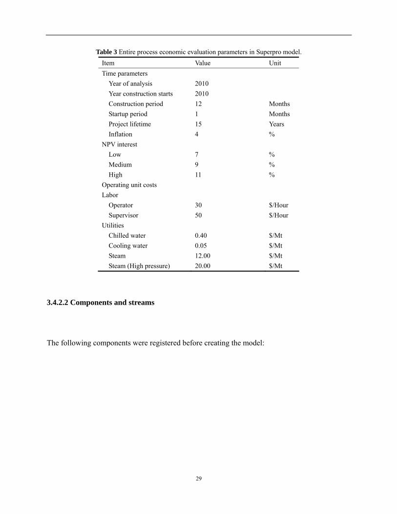
The economic evaluation parameters for the entire process are listed in Table 3:
29
Table 3 Entire process economic evaluation parameters in Superpro model. Item Value Unit Time parameters
Year of analysis 2010 Year construction starts 2010 Construction period 12 Months Startup period 1 Months Project lifetime 15 Years Inflation 4 %
NPV interest Low 7 % Medium 9 % High 11 %
Operating unit costs Labor
Operator 30 $/Hour Supervisor 50 $/Hour
Utilities Chilled water 0.40 $/Mt Cooling water 0.05 $/Mt Steam 12.00 $/Mt Steam (High pressure) 20.00 $/Mt
3.4.2.2 Components and streams
The following components were registered before creating the model:

30
Table 4 Component registration for Superpro model. Name MW (g/gmol)Water 18.02Dry Yeast 180.16Non-starch Polysaccharides 18.02Oil 18.02Other Solids 18.02Yeast Dry Matter 18.02Protein-insoluble 180.16Protein-soluble 180.16Ethanol 46.07CO2 44.01
In this model, Ethanol, DDGS and CO2 were classified as revenue streams, and all input streams
were classified as raw material streams. Purchasing price of raw material streams and selling
price of revenue streams were calculated according to the contents’ prices, except for Ethanol
and CO2, the selling prices were set to 0.724419 $/kg and 0.011955 $/kg, respectively, as listed
in Table 1.
3.4.2.3 Equipment sizing
Yeast tank The Yeast tank is a continuous storage blending tank in Superpro Designer’s
databank. The final temperature was set to 42.34℃, and the pressure is 1.013 bar. The specific
power consumption was set to 0.5 kW/m3. The residence time of the Yeast tank was set to 40 h,
with a 90% working volume of 2669.34 L. Working volume ranges from 15~90% of the total
volume. The Volume of the tank is 2.97 m3, with a height of 3.24 m and diameter of 1.08 m.

31
Yeast pump The fermentor yeast pump has a pressure change of 150 psi and a calculated
volumetric flow rate of 0.06716 m3/h. The operating power is 0.055 kW and the efficiency is
35%.
Air filter The Air filter is an air filtration unit in Superpro Designer’s databank with an air flow
of 4600.369 m3/h. The size is calculated automatically by Superpro Designer according to the
design flow rate.
Fermentor The fermentor is a continuous stoichiometric fermentor in Superpro Designer’s
databank. The fermentor was operated under 30 ℃ and atmospheric pressure, with a specific
power consumption of 0.028 kW/m3, and an aeration rate of 0.01 VVM. The residence time
varied according to different fermentation conditions applied. The working volume is set to 83%
of the total volume. 98.5% of CO2, 2.55% of ethanol and 0.23% water was emitted from the
fermentor. The fermentor is 29.8 m in height and 19.9 m in diameter, and the maximum volume
is 14000 m3.
CO2 scrubber The CO2 scrubber is an absorption unit in Superpro Designer’s databank. It was
designed to remove 99.8% dry yeast, 0.1% CO2 and 59% water from the feed. The design
component is ethanol, diffusivity in gas phase is 123 cm2/s, and 13 cm2/s in liquid phase. The CF
was set to be 155, with the total specific surface of 190 m2/m3, nominal diameter of 0.00762 m,

32
and critical surface tension of 40 dyn/cm. The column is 8.571 m in height and 1.411 in diameter.
Beer pump The beer yeast pump has a pressure change of 50 psi and a calculated volumetric
flow rate of 137.409 m3/h. The operating power is 18.798 kW and the efficiency is 70%.
Heat exchanger The heat exchanger has a countercurrent flow type with a correction factor of
1.00. The heat transfer coefficient was set to 140 btu/h-ft2-℃. The cold stream outlet temperature
was set to 95 ℃, and the minimum achievable temperature is 5 ℃. The maximum heat transfer
surface was set to 929.03 m2 and the exchanger type is plate and frame.
Beer column feed pump The beer column feed pump has a pressure change of 45 psi and a
calculated volumetric flow rate of 117.449 m3/h. The operating power is 14.460 kW and the
efficiency is 70%.
Beer column The beer column is a distillation unit in Superpro Designer’s databank. It was
designed to separate 100% CO2, 99.7% ethanol and 12.44% water from the beer. The reflux ratio
was calculated to be 0.121. The column pressure was set to 1.03 bar and vapor linear velocity
was set to 1.618 m/s. The stage efficiency was set to 36.4%. The condenser is operated at 104 ℃
and the Reboiler is operated at 115.33 ℃. The column is 15.545 m in height and 2.803 m in
diameter with a stage height of 0.457 m and the design pressure of 1.48 atm.

33
DDGS pump The DDGS pump has a pressure change of 50 psi and a calculated volumetric
flow rate of 106.221 m3/h. The operating power is 14.531 kW and the efficiency is 70%.
Stream mixer The stream mixer is a 3-stream mixing unit in Superpro Designer’s databank.
The calculated operating mass flow rate is 36233.63 kg/h.
Rectifier The rectifier is a distillation unit in Superpro Designer’s databank. It was designed to
separate 99.44% ethanol and 11.46% water from the feed. The reflux ratio was calculated to be
0.126. The column pressure was set to 1.03 bar and vapor linear velocity was set to 0.678 m/s.
The stage efficiency was set to 40%. The condenser is operated at 95 ℃ and the Reboiler is
operated at 114.36 ℃. The column is 16.612 m in height and 3.153 m in diameter with a stage
height of 0.593 m and the design pressure of 2 bar.
Molecular sieves The rectifier is a 2-way component splitting unit in Superpro Designer’s
databank. It was designed to split 16.2% ethanol and 97% water from the feed to the top stream.
The operating power was set to 14.4 kW.
Recycle pump The recycle pump has a pressure change of 50 psi and a calculated volumetric
flow rate of 1.712 m3/h. The operating power is 0.234 kW and the efficiency is 70%.
Stripper feed pump The stripper feed pump has a pressure change of 50 psi and a calculated

34
volumetric flow rate of 13.904 m3/h. The operating power is 1.902 kW and the efficiency is 70%.
Stripper The stripper is a distillation unit in Superpro Designer’s databank. It was designed to
separate 99% ethanol and 11.46% water from the feed. The reflux ratio was calculated to be
0.125. The column pressure was set to 1.03 bar and vapor linear velocity was set to 3 m/s. The
stage efficiency was set to 40%. The condenser is operated at 90 ℃ and the Reboiler is operated
at 114 ℃. The column is 12.344 m in height and 0.590 m in diameter with a stage height of
0.457 m and the design pressure of 1.5 bar.
Storage tank The storage tank is a continuous storage flat bottom tank in Superpro Designer’s
databank. The final temperature was set to 42℃, and the pressure is 1.013 bar. It has a 90%
working volume of 433251 L. Working volume ranges from 15~90% of the total volume. The
Volume of the tank is 481.39 m3, with a height of 13.484 m and diameter of 6.742 m.
3.4.2.4 Purchase cost of equipments
Purchase costs as well as required parameters were presented in Table 5:

35
Table 5 Parameters for the calculation of equipment purchase cost. In Material column, CS stands for Carbon Steel, SS304 stands for Stainless Steel 304, SS316 stands for Stainless Steel 316.
Equipment name Cost estimation option
Material Material factor
Installation cost (× PC)
V-104 (Yeast tank) User-defined model SS304 1.00 2.00 GP-101 (Yeast pump) Set by user SS316 1.00 2.00 AF-101 (Air filter) Built-in model CS 1.00 2.00 V-101 (Fermentor) User-defined model SS316 1.00 2.00 C-104 (CO2 scrubber) User-defined model SS304 2.40 2.00 PM-101 (Beer pump) Set by user SS316 1.00 2.00 HX-103 (Heat exchanger) User-defined model CS 1.00 0.50 PM-102 (Beer column feed pump) Set by user SS316 2.05 2.00 C-101 (Beer column) User-defined model SS304 3.88 2.00 PM-103 (DDGS pump) Set by user SS316 2.05 2.00 MX-102 (Stream mixer) Built-in model CS 1.00 2.00 C-102 (Rectifier) User-defined model SS304 1.00 2.00 CSP-101 (Molecular sieves) User-defined model CS 1.00 2.00 PM-104 (Recycle pump) Set by user SS316 2.05 2.00 PM-105 (Stripper feed pump) Set by user SS316 2.05 2.00 C-103 (Stripper) User-defined model SS304 3.86 2.00 V-103 (Storage tank) User-defined model SS304 1.00 2.00
For the cost estimation option:
1. Set by user means you can specify the purchase cost yourself;
2. Built-in model is specific to this type of equipment;
3. User-defined model means you can define the parameters of a power-law model that will
determine the cost of the equipment.
It should be mentioned that all the costs were calculated for the reference year of 2010. The
user-specified cost can either be fixed and independent of the year of analysis for the design case
or adjustable to inflation according to a reference year.

36
The user-defined cost model is of the following power-law form:
a
oo Q
QCPC ⎟⎟⎠
⎞⎜⎜⎝
⎛= (3)
Where Co is the base cost, Qo is the base capacity, and a is the exponent of the power law
function. In cases where the capacity variable Q needs to span a wide range of values, the total
range is broken down into several intervals and a set of parameters a, Co and Qo is supplied for
each interval. The specification of a user-defined cost model must also be accompanied by the
calendar year (the reference year 2010 were used for this model) for which the cost estimates of
the model are accurate, in order for the program to be able to adjust for inflation. Parameters of
each unit procedure for the purchase cost model are listed in Table 6:
Table 6 Parameters of unit procedures for which the user-defined model was used to determine the purchase
cost in Superpro Model. Equipment name Low end (m3) High end (m3) Qo (m3) Base cost ($) a V-104 (Yeast tank) 0 1000 2.97 114700 0.6 V-101 (Fermentor) 100 14000 10446.31 2811200 0.6 C-104 (CO2 scrubber) 0 10000 13.41 91300 0.6 HX-103 (Heat exchanger) 0 1000 402.34 458900 0.6 C-101 (Beer column) 0 50000 96.57 597000 0.6 C-102 (Rectifier) 1 10000 113.57 254000 0.6 CSP-101 (Molecular sieves) 10000 720000 22924.40 1717700 0.6 C-103 (Stripper) 0 100 3.72 168200 0.6 V-103 (Storage tank) 0 1000 481.39 93400 0.6
For example, the fermentor has a volume of 9237.69 m3, then its purchase cost can be calculated
as following:

37
$261100031.10446
69.923728112006.0
=⎟⎠⎞
⎜⎝⎛×=FermentorPC .
3.4.2.5 Profitability calculations
In profitability analysis, the following items that are essential for economic analysis were
calculated:
Annual production rate = Production rate × Annual operating time;
Annual operating cost = Raw materials cost + Labor cost + Facility cost + Utilities cost;
Unit production cost =rate production Annual
cost operating Annual ;
Total product sales =∑ ×i
)rate production Annualprice Selling( ii , (i = Ethanol, DDGS, CO2);
cost operating AnnualCostcost productionUnit breakdownCost i
i ×= , (i = raw materials, labor,
facility, utilities);
Ethanol yield =ionconcentrat glucose Final -ionconcentrat glucose Initial
ionconcentrat ethanol Final ;
For example, in the first repeat of condition Aa (Aa1):
Annual production rate = 17644.098 kg/h × 7920 h = 139741258.989 kg ethanol/year;
Annual operating cost = 218743308 $ + 1980000 $ + 9071000 $ + 10192335 $ = 239986643 $;
Unit production cost =ethanol kg 989139741258.$ 239986643 = 1.7174 $/kg ethanol;
Total product sales = 0.724419 $/kg ×139741258.99 kg/year + 0.022417 $/kg × 813729597.12

38
kg/year + 0.011955 $/kg ×184208737.68 kg/year = 121674814.93 $/year;
Cost breakdown of ethanol = 1.7174 $/kg ×$ 239986643$ 218743308 = 1.5653 $/kg;
Ethanol yield =g/L 15.37-g/L 302.15
g/L 125.95 = 0.4392.
It should be noticed that values presented in next chapter is the average of two repeats of one
certain condition.

39
3.5 Aspen Plus model
3.5.1 Process description
As mentioned before, since the academic version of Superpro Designer v7.0 used in the first
model has a disadvantage that the number of unit procedures is limited to be less than 25 in one
process model, therefore the liquefaction and saccharification sections of an ethanol producing
were purposely ignored, as well as downstream treatment of DDGS stream and recycle streams.
Also, glucose, an important intermediate product produced from the saccharification section and
consumed in the fermentation section, is directly used as process feed of the entire model. This
makes the estimated costs too high to be compared with market values. In order to perform the
process simulation in a more accurate model, Aspen Plus was introduced to create a model of an
entire ethanol fermentation process.
A brief demonstration of the Aspen Plus process model used in this study is shown in Figure 4,
The PFD of this model is shown in Appendix B. The original model was created based on Taylor
et al. (2000). Some alternative branches in the original model for possible future scale-up or
scale-down were deleted, only necessary components for this study was included or created.
Model settings used for process simulation and economic evaluation were determined based on
Taylor et al.’s (2000) model or from experimental data collected in laboratories (Lin et al., 2010),
and are listed in Appendix C. This simulation focused on studying the technical and economical

40
effects of the glucose feeding concentration and redox potential control on the ethanol production
under VHG conditions, and the estimated unit production cost of ethanol can also be compared
with market price.
GrainMilling Liquefaction Saccharification
FermentorAge TankDegasCondense
Beer Column RectifierMolecular Sieve
Centrifuge EvaporationDDGS Dryer
CO2Scrubber
CO2
Ethanol
DDGS
Figure 4 Aspen Plus process model for redox potential-controlled very-high-gravity ethanol fermentation
(modified from Taylor et al. (2000))
The same experimental conditions were applied in this model for simulation in order to compare
the two models. The glucose concentration in the feed to fermentor was shown in Table 2, the
same conditions were applied in the previous Superpro model.
In this model, the glucose concentration in the feed of fermentor was manipulated by varying the

41
starch content in the Grain stream feeding to the Milling module as shown in Figure 4. The
Milling module is a separation process while the Liquefaction module is a heating process, in
both of which no chemical reactions were defined. However, in the Saccharification module, one
reaction was defined:
Glucose WaterStarch →+ (4)
Equation 4 defined the molecular relation of the reaction from starch to glucose, which means
one molecule of starch one molecule of water generates one molecule of glucose. Starch in this
model is a predefined pure component with a molecular weight of 162.14.
In the fermentor, two reactions were defined:
YDM Ethanol CO Glucose 2 βαα ++→ (5)
Protein 13635848.1YDM → (6)
α, β in Equation 5 are the molar coefficients of the first reaction that were determined based on
results of lab fermentation experiments before simulation, as described in 3.3.1 “Process
modeling using Superpro Designer v7.0”. Whereas 1.13635848 in Equation 6 is the predefined
mass coefficient according to predefined molecular weights of the components YDM and Protein.
YDM in Equation 5 and Equation 6 is short for Yeast Dry Matter.
After fermentation, the beer is sent to an aging tank, where most of CO2 (over 98.7% in feed) is
separated from the beer, and then is sent into a degasser where CO2 in the beer is further
removed (70% of the left over CO2 in the beer). After that, the beer is sent into the distillation

42
section which includes a beer column and a rectifier. The top output stream of the degasser is
condensed by a condenser in order to recover most of ethanol (around 80% in feed) in it. This
condensed stream is also sent to the beer column for further separation.
The beer column is a primary separation process unit to separate most of ethanol (over 99.7% of
ethanol in its feed stream) from the fermentor’s output stream together with a certain amount of
water. This stream which is mainly composed of ethanol and water is then sent to a rectifier
connected with a molecular sieve for further ethanol-water separation. The using of molecular
sieve is to overcome the limitation of distillation process to yield main product stream with high
ethanol concentration. Molecular sieves are applied to separate the azeotrope of water and
ethanol (ethanol : water = 95.6 : 4.4 in mass), with recycling, ethanol concentration in the output
stream reaches to over 99.25% in mass.
The bottom stream of the beer column is sent to a centrifuge and then a dryer to yield DDGS,
which is the main byproduct of this ethanol producing process. It should be mentioned that under
actual circumstances, protein and other solids contents in the feed stream to the Milling section
are proportionally changed while varying the starch content. However, since variations of protein
and other solids contents in the feed stream have no significant influence on economical
evaluation results, they remained unchanged in simulated scenarios in order to precisely
manipulate the glucose concentration in feed stream of the fermentor.

43
The top output streams of the aging tank and condenser which are rich in CO2 are sent to a CO2
scrubber where liquid portion of the feeds are absorbed by water and major portion of CO2
(over 99.8%) produced during the fermentation process is gathered for further emission, capture
or deep injection.
In the Aspen Plus model, CO2 produced during the fermentation process is assumed to be
captured after treatment in the CO2 scrubber and sold as another byproduct.
3.5.2 Economic evaluation
3.5.2.1 Economic evaluation parameters defined in Aspen IPE
Since Aspen Plus can not directly perform economic evaluations itself, another Aspen software
was introduced. To perform economic evaluation for a existed process model after the simulation
was correctly completed, simulation results were sent to Aspen IPE for economic evaluations,
and required or default parameters were shown in the following tables:

44
Table 7 Investment parameters used in Aspen Plus model. Name Values Units INVESTMENT PARAMETERS
Project Capital Escalation 5 Percent/Period Products Escalation 5 Percent/Period Raw Material Escalation 3.5 Percent/Period Operating and Maintenance Labor Escalation 3 Percent/Period Utilities Escalation 3 Percent/Period
PROJECT CAPITAL PARAMETERS Working Capital Percentage 5 Percent/Period
OPERATING COSTS PARAMETERS Operating Supplies 25 Cost/Period Laboratory Charges 25 Cost/Period Operating Charges 25 Percent/Period Plant Overhead 50 Percent/Period G and A Expenses 8 Percent/Period
FACILITY OPERATION PARAMETERS Facility type Chemical Processing Facility Operating mode Continuous Processing - 24 Hours/Day Length of Start-up Period 20 Weeks Operating Hours per Period 7920 Hours/Period
Process Fluids Liquids and Solids
Table 8 Operating unit costs defined in evaluating the Aspen Plus model. Name Values Units LABOR UNIT COSTS
Operator 20 Cost/Operator/Hour Supervisor 35 Cost/Supervisor/Hour
UTILITY UNIT COSTS
Electricity 0.0354 Cost/KWH
Potable Water 0 Cost/M3 Fuel 0.002427 Cost/MEGAWH
Instrument Air 0 Cost/M3

45
Table 9 General specifications defined in evaluating the Aspen Plus model. Name Settings Process Description Proven process Process Complexity Typical Process Control Digital PROJECT INFORMATION
Project Location North America Project Type Grass roots/Clear field Contingency Percent 18 Estimated Start Day of Basic Engineering 1 Estimated Start Month of Basic Engineering JAN
Estimated Start Year of Basic Engineering 10 Soil Condition Around Site SOFT CLAY
EQUIPMENT SPECIFICATION
Pressure Vessel Design Code ASME Vessel Diameter Specification ID
P and I Design Level FULL
3.5.2.2 Components and streams
Components used in the Aspen Plus model is shown in Table 10:
Table 10 Component registration for Aspen Plus model. Name Molecular weightWater 18.02Ethanol 46.07CO2 44.01Glucose 180.156Starch 162.141Protein 132.115Oil 132.115YDM 150.130Cpoly 147.128

46
Three product streams were defined in Aspen IPE: Ethanol, DDGS and CO2. Selling prices of
product streams were calculated according to prices listed in Table 1.
3.5.2.3 Equipments
When creating the Aspen Plus model, operating conditions were defined, as well as some sizing
information, and are shown in Appendix C. However, after simulation results were sent to Aspen
IPE, equipment mapping and sizing can be automatically performed by Aspen IPE. In this study,
default settings in Aspen IPE were used when performing equipment mapping and sizing, unless
the required sizing information was already set in operating conditions.
3.5.2.4 Profitability calculations
Simulation results of Aspen Plus model used in this study were obtained using almost the same
calculation methods as the Superpro model, except for the calculation of Annual operating cost:
Annual operation cost = Subtotal operating cost + G and A cost;
Subtotal operating cost = Total raw materials cost + Total utilities cost + Operating labor cost +
Maintenance cost + Operating charges + Plant overhead;
G and A cost = 0.08 × Subtotal operating cost.
47
3.6 Reactions and coefficients
In simulation, different fermentation conditions were applied by manipulating the reaction
coefficients α, β in Equation 1 and 5, as well as its reaction extent. α is the molar ratio of yield
ethanol over depleted glucose that were measured by lab experiments under certain applied
conditions, whereas β is dependent to α to ensure mass balance of the reaction.
1.13635848 in Equation 6 is in fact an approximate value of the fractional ratio of YDM and
Protein’ molecular weight, which are 150.130 and 132.115, respectively. Because a fraction can
not be specified as reaction coefficients in a simulator.
The reaction extent of Equation 1 is the mass ratio of depleted glucose over total feed glucose
measured under certain applied conditions. Reaction extent of Equation 2 and 6 is fixed to 0.6,
according to Kwiatkowski et al.’s (2006). The reaction extent of Equation 5 was set to 0.99,
according to Taylor et al. (2000).

48
CHAPTER 4 RESULTS AND DISCUSSION
By manipulating mass composition of glucose in feed of fermentor in both models, and applying
different fermentation conditions to the two models, VHG fermentations were simulated by two
process models. Though these fermentation conditions were only performed under laboratory
experiments, therefore there might be some inaccuracies from the simulated scenarios to an
actual VHG fermentation process, these results are still helpful for future studies on VHG
fermentation. In addition, economical effects of different fermentation conditions were also
compared based on economic evaluation results.
4.1 Experimental data and parameter calculation
The experimental data provided by Lin et al. (2010) that were used in process simulations were
presented in Appendix A. To apply different fermentation conditions to the two models, certain
calculations are required to convert these experimental data to model parameters. The
calculations were briefly discussed in section “3.6 Reactions and coefficients”, calculated values
that can be used as model parameters are shown in Table 11:

49
Table 11 Parameters evaluated from experimental data that are required in modeling. In the first column of scenarios, different glucose concentrations in feed stream are denoted as: A = 300±6.42 g/L, B = 250±3.95 g/L,
C = 200±4.99 g/L. Different redox potential control levels are denoted as: a = no control, b = -150 mV, c = -100 mV. 1 and 2 stand for different repeats of an individual scenario.
Conditions Residence time (h) Reaction 1 (or 4) extent α β in reaction 1 β in reaction 4Aa1 53 0.9491 1.7175 1.4123 0.1695 Aa2 53 0.9302 1.7966 1.0165 0.1220 Ab1 53 0.9350 1.7944 1.0280 0.1234 Ab2 53 0.9843 1.8635 0.6824 0.0819 Ac1 53 0.9226 1.6402 1.7988 0.2159 Ac2 53 0.9931 1.5775 2.1121 0.2535 Ba1 47 1 1.9884 0.0581 0.0070 Ba2 47 1 1.8950 0.5249 0.0630 Bb1 41 1 1.8907 0.5466 0.0656 Bb2 41 1 1.8905 0.5472 0.0657 Bc1 41 1 1.9202 0.3989 0.0479 Bc2 41 1 1.9588 0.2059 0.0247 Ca1 29 1 1.8244 0.8778 0.1054 Ca2 29 1 1.8186 0.9066 0.1088 Cb1 29 1 1.8787 0.6065 0.0728 Cb2 29 1 1.8122 0.9388 0.1127 Cc1 29 1 1.7683 1.1582 0.1390 Cc2 29 1 1.8399 0.8004 0.0961
For the condition “Aa1”:
Residence time = Fermentation time + 5 hours (Maintenance and cleaning) = 48 + 5 = 53 hours;
Reaction 1 (or 4) extent
=15.302
37.1515.302ionconcentrat glucose Initial
ionconcentrat glucose Final-ionconcentrat glucose Initial −= = 0.9491;
( )16.180
)37.1515.302(07.46
95.125
MWionconcentrat glucose Final-ionconcentrat glucose Initial
MWionconcentrat ethanol Final
Glucose
Ethanol
−==α
= 1.7175;

50
02.187175.1)01.4407.46(16.180
MW)MWMW(MW
MatterDry Yeast
COEthanolGlucose1Reaction
2 ×+−=
×+−=
αβ = 1.4123;
13.1507175.1)01.4407.46(16.180
MW)MWMW(MW
YDM
COEthanolGlucose4Reaction
2 ×+−=
×+−=
αβ = 0.1695.
It should be mentioned that since β is dependent to α, therefore for each applied condition in one
model, only one pair of α and β can be specified.

51
4.2 Results of process simulation using Superpro Designer v7.0
4.2.1 General results
In the process simulation, two variables are introduced: initial glucose concentration to the
fermentor was obtained from experiments: 200±4.99, 250±3.95 and 300±6.42 g/L, along with
different levels of redox potential control. The summarized results of economic evaluation are
shown in Table 12. The breakdown of unit production cost for each basic case is shown in Table
13. The annual operating cost in Table 12 is composed of raw materials, facility, labor and utility,
as listed in the first column of Table 13. As for one experimental condition, two repeats were
applied, therefore evaluation results discussed in following parts of this chapter were actually
averages of the two repeats’ estimated values.
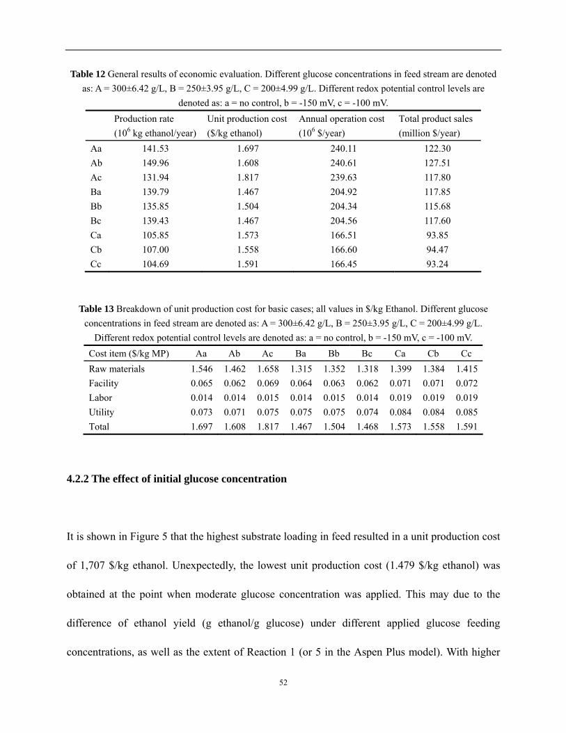
52
Table 12 General results of economic evaluation. Different glucose concentrations in feed stream are denoted as: A = 300±6.42 g/L, B = 250±3.95 g/L, C = 200±4.99 g/L. Different redox potential control levels are
denoted as: a = no control, b = -150 mV, c = -100 mV.
Production rate (106 kg ethanol/year)
Unit production cost ($/kg ethanol)
Annual operation cost (106 $/year)
Total product sales (million $/year)
Aa 141.53 1.697 240.11 122.30 Ab 149.96 1.608 240.61 127.51 Ac 131.94 1.817 239.63 117.80 Ba 139.79 1.467 204.92 117.85 Bb 135.85 1.504 204.34 115.68 Bc 139.43 1.467 204.56 117.60 Ca 105.85 1.573 166.51 93.85 Cb 107.00 1.558 166.60 94.47 Cc 104.69 1.591 166.45 93.24
Table 13 Breakdown of unit production cost for basic cases; all values in $/kg Ethanol. Different glucose concentrations in feed stream are denoted as: A = 300±6.42 g/L, B = 250±3.95 g/L, C = 200±4.99 g/L.
Different redox potential control levels are denoted as: a = no control, b = -150 mV, c = -100 mV. Cost item ($/kg MP) Aa Ab Ac Ba Bb Bc Ca Cb Cc Raw materials 1.546 1.462 1.658 1.315 1.352 1.318 1.399 1.384 1.415Facility 0.065 0.062 0.069 0.064 0.063 0.062 0.071 0.071 0.072Labor 0.014 0.014 0.015 0.014 0.015 0.014 0.019 0.019 0.019Utility 0.073 0.071 0.075 0.075 0.075 0.074 0.084 0.084 0.085Total 1.697 1.608 1.817 1.467 1.504 1.468 1.573 1.558 1.591
4.2.2 The effect of initial glucose concentration
It is shown in Figure 5 that the highest substrate loading in feed resulted in a unit production cost
of 1,707 $/kg ethanol. Unexpectedly, the lowest unit production cost (1.479 $/kg ethanol) was
obtained at the point when moderate glucose concentration was applied. This may due to the
difference of ethanol yield (g ethanol/g glucose) under different applied glucose feeding
concentrations, as well as the extent of Reaction 1 (or 5 in the Aspen Plus model). With higher

53
glucose feeding concentration (300±6.42 g/L) and the osmotic pressure caused by the very high
glucose concentration, yeast cells need longer time and more energy to adapt themselves to the
extreme conditions, therefore the ethanol yield, also known as the substrate utilization rate (g
ethanol/g glucose), decreased, therefore reduced the profitability of the process. In fact, in all
applied experiment conditions with 300±6.42 g/L as the glucose feeding concentration to the
fermentor, the residual glucose concentration in the beer remains at 14.39 g/L in average, even
after the longest fermentation time (48 hours), this means the substrate in feed was not efficiently
utilized, or reflected as a smaller Reaction 1 (or 4) extent. Fermentation with higher glucose
loading needs longer fermentation time, and the longer fermentation time may reduce the VHG
fermentation efficiency. Moreover, high residual glucose concentration in beer means a small
Reaction 1 (or 4) extent as a sign of a waste of unspent glucose, and imposes difficulty of
downstream processing, therefore less profitable even though the annual production rate is 5 a
little higher (2%) than scenarios with glucose feeding concentration at 250±3.95 g/L. Under the
conditions with low glucose feeding concentrations (200±4.99 g/L), despite that glucose can be
completely utilized by yeast cells and hence shorter fermentation time was needed, the low
glucose feeding concentration still diminishes the efficiency of the entire process, making it not
economically preferable.
Usually, VHG fermentation means bio-ethanol fermentation with initial glucose concentration
greater than 250 g/L. It was expected that VHG fermentation may reduce the unit production cost
due to high ethanol productivity and high ethanol concentration in product, but the simulation

54
results suggested otherwise in the economical aspect.
Figure 5 Effects of initial glucose concentration on unit production cost and annual ethanol production rate in
Superpro model
Residence time also influences the ethanol yield in fermentor and thus the economical evaluation
results. With longer residence time, yeast cells are capable of converting more substrate to
product, therefore increase the utilization ratio of substrate. However, there should be an
optimum residence time for a certain fermentation process. Longer residence time reduces the

55
efficiency of the entire fermentation process, causing the increase of unit production cost.
4.2.3 The effect of redox potential control
To study the effect of redox potential control on fermentation process and its impact on
profitability, two redox potential levels controlled at -100 mV and -150 mV, respectively, were
implemented during VHG fermentation and their effects on fermentation were compared to the
case of no redox potential control. Results suggested that the redox potential control can
stimulate yeast performance and improve fermentation efficiency, thus resulting in higher profit.
At lower glucose feeding concentrations (200±4.99 g/L and 250±3.95 g/L), redox potential
control seemed have no significant influence on ethanol yield comparing to the results of high
glucose feeding concentration. The effect of redox potential control on ethanol yield shown in
Figure 6a is consistent with the conclusion of former observations (Figures 3) that glucose
feeding concentration at 250±3.95 g/L results in the highest conversion rate due to the optimal
fermentation conditions. The low ethanol yield might be attributed to the osmotic stress resulting
from the presence of excess amount of glucose when 300±6.42 g/L glucose was fed to fermentor.
Nevertheless, when redox potential was controlled at -100 mV, the ethanol yield decreased
significantly by 8.4% from 0.4493 to 0.4114 g ethanol/g glucose. In contrast, when redox
potential was controlled at -150 mV, the ethanol yield increased from 0.4114 to 0.4677, even
4.1% greater than that when no redox potential control was applied. From Figure 6a, one can

56
conclude that redox potential control has little to no noticeable effect on ethanol yield at glucose
feeding concentration no greater than 250 g/L. However, a remarkable impact on ethanol yield
was observed at 300±6.42 g glucose/L. This result is consistent with Lin et al. (2010) that under
VHG conditions, maintaining redox potential at -150 mV could obtain better ethanol yield. This
is to say, redox potential control has significant effects on VHG fermentation process.
Controlling redox potential at different levels may result in different ethanol yields. The optimal
redox potential level could be further refined for a certain fermentation condition.
It is possible that the effect of redox potential control on VHG fermentation system is reflected
by ethanol yield:
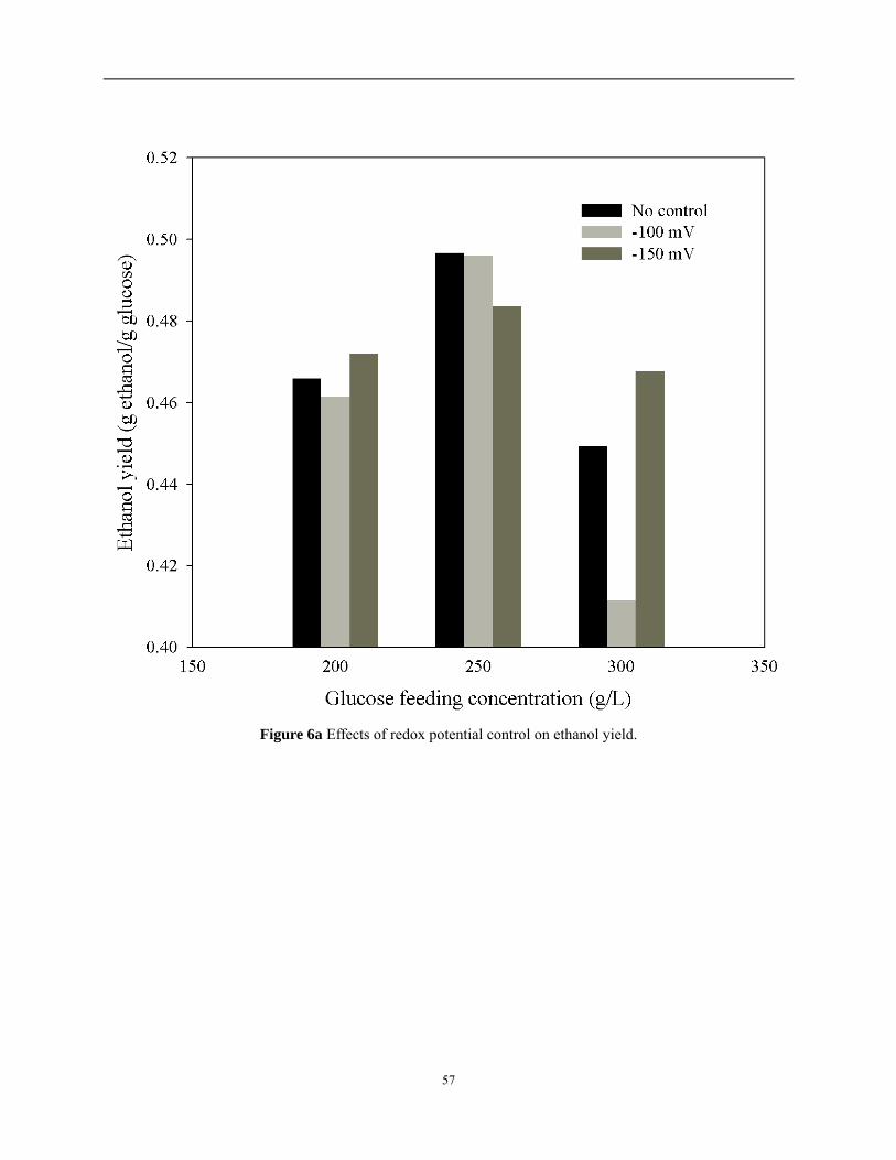
57
Figure 6a Effects of redox potential control on ethanol yield.

58
Figure 6b Effects of redox potential control on ethanol unit production cost in Superpro model.
The effects of redox potential and glucose feed on the ethanol unit production cost are shown in
Figure 6b. The unit production cost decreased dramatically from 1.817 $/kg to 1.608 $/kg under
300±6.42 g/L glucose feeding concentration when redox potential was controlled from -100 mV
to -150 mV. This result is consistent with the result shown in Figure 6a that ethanol yield
increases from 0.4114 to 0.4677 under these conditions.

59
4.3 Process simulation using Aspen Plus 2006
4.3.1 General results
During the process simulation by Aspen Plus, the effects of same glucose feeding concentration
(200±4.99, 250±3.95 and 300±6.42 g/L) and same redox potential settings (no control, -150 and
-100 mV) were investigated as I did in the Superpro model. The summarized results of economic
evaluation are shown in Table 14, the breakdown of unit production cost for each investigated
case is listed in Table 15.
Table 14 Results of economic evaluation. Different glucose concentrations in feed stream are denoted as: A = 300±6.42 g/L, B = 250±3.95 g/L, C = 200±4.99 g/L. Different redox potential control levels are denoted as:
a = no control, b = -150 mV, c = -100 mV.
Production rate (106 kg ethanol/year)
Unit production cost ($/kg ethanol)
Annual operation cost (106 $/year)
Total product sales (106 $/year)
Aa 124.65 0.825 102.87 117.97 Ab 131.93 0.780 102.93 119.45 Ac 115.71 0.888 102.79 116.36 Ba 118.98 0.757 90.08 106.40 Bb 115.84 0.777 90.06 106.24 Bc 118.84 0.758 90.08 106.39 Ca 86.54 0.885 76.56 84.42 Cb 87.68 0.873 76.56 84.53 Cc 85.71 0.893 76.56 84.34

60
Table 15 Breakdown of unit production cost for each case; all values in $/kg ethanol. Different glucose concentrations in feed stream are denoted as: A = 300±6.42 g/L, B = 250±3.95 g/L, C = 200±4.99 g/L.
Different redox potential control levels are denoted as: a = no control, b = -150 mV, c = -100 mV. Cost item ($/kg Ethanol) Aa Ab Ac Ba Bb Bc Ca Cb Cc Raw material cost 0.738 0.698 0.795 0.676 0.694 0.676 0.788 0.777 0.795Utilities cost 0.012 0.012 0.012 0.011 0.011 0.011 0.012 0.012 0.012Operating Labor Cost 0.007 0.007 0.008 0.008 0.008 0.008 0.011 0.010 0.011Maintenance Cost 0.001 0.001 0.001 0.001 0.001 0.001 0.001 0.001 0.001Operating Charges 0.002 0.002 0.002 0.002 0.002 0.002 0.003 0.003 0.003Plant Overhead 0.004 0.004 0.004 0.004 0.004 0.004 0.006 0.006 0.006G and A Cost 0.061 0.058 0.066 0.056 0.058 0.056 0.066 0.065 0.066Total 0.825 0.780 0.888 0.757 0.777 0.758 0.885 0.873 0.893
4.3.2 Sales analysis
The sales analysis results of all studied scenarios with different glucose feeding concentrations
and different redox potential settings are listed in Table 16. Ethanol is the main product of the
process, while DDGS and CO2 are byproducts, selling prices of which are presented in Table 1.

61
Table 16 Sales analysis for each applied condition; Different glucose concentrations in feed stream are denoted as: A = 300±6.42 g/L, B = 250±3.95 g/L, C = 200±4.99 g/L. Different redox potential control levels are
denoted as: a = no control, b = -150 mV, c = -100 mV.
Total operating cost (million $/year)
Total product sales (million $/year)
Payout period (years)
Aa 102.87 117.97 6.08 Ab 102.93 119.45 5.71 Ac 102.79 116.36 6.59 Ba 90.08 106.40 5.32 Bb 90.06 106.24 5.35 Bc 90.08 106.39 5.32 Ca 76.56 84.42 8.47 Cb 76.56 84.53 8.39 Cc 76.56 84.34 8.52
Payout Period is the expected number of years required to recover the original investment in the
project. This parameter indicates the length of time that the facility needs to operate in order to
recover the initial capital investment (total capital cost plus working capital). The results shown
in Figure 7 suggested that for an ethanol plant with a capacity of 85~130 million kg ethanol/year,
maintaining the glucose feeding concentration to the fermentor at around 250 g/L resulted in the
shortest payout period of 5.33 years in average, with or without redox potential control. If
300±6.42 g/L glucose feeding concentration to the fermentor is applied, it is essential to have the
redox potential only controlled at -150 mV in the fermentor to limit the process payout period
within 6 years. In addition, fermentation processes with glucose feeding concentration at around
200 g/L to the fermentor were estimated to have payout period of over 8 years under all
evaluated scenarios. This makes the process much less profitable comparing to scenarios with
higher glucose feeding concentrations.

62
Figure 7 Sales analysis of payout period on different glucose feeding concentrations and redox potential
controls in Aspen Plus model.
4.3.3 Effect of glucose feeding concentration
Results with similar trends were obtained from the Aspen Plus model, as shown in Figure 8, the
highest glucose loading in feed did not result in the lowest unit production cost, and the lowest

63
unit production cost (0.764 $/kg ethanol) was obtained when the glucose feeding concentration at
250±3.95 g/L was applied. Besides the difference of actual unit production cost values,
Production rate of scenarios with glucose feeding concentration at 300±6.42 g/L is 5% higher
than scenarios with glucose feeding concentration at 250±3.95 g/L.
Figure 8 Effect of glucose feeding concentration on Production rate and unit production cost in Aspen model.
The selling price of the DDGS stream was calculated based on its moisture content and the dry

64
DDGS price, which was presented in Table 1. In addition, higher glucose feeding concentration
results in higher biomass content thus less moisture in DDGS as a byproduct stream, therefore
higher selling price for DDGS as another revenue stream, but still not significant to make the
whole process more profitable than the scenarios with moderate glucose feeding concentration
(250±3.95 g/L).
The influence of glucose feeding concentration on ethanol yield along with unit production cost
is shown in Figure 9, values used in the figure were averages of all investigated conditions under
one certain glucose feeding concentration, difference of redox potential control effects were not
considered here. The lowest unit production cost (0.764 $/kg ethanol) and highest ethanol yield
(0.4920 g ethanol/g glucose) were achieved when the moderate glucose feeding concentration
(250±3.95 g/L) were applied. In contrast, high glucose feeding concentration (300±6.42 g/L) led
to the lowest ethanol yield (0.4428 g ethanol/g glucose in average), and low glucose feeding
concentration (200±4.99 g/L) resulted in the highest unit production cost (0.884 $/kg ethanol in
average), both of which are not economically preferable. This result suggests that under
moderate glucose feeding concentration, the fermentation system neither produces biomass more
than it needs, nor waste glucose from the feed.
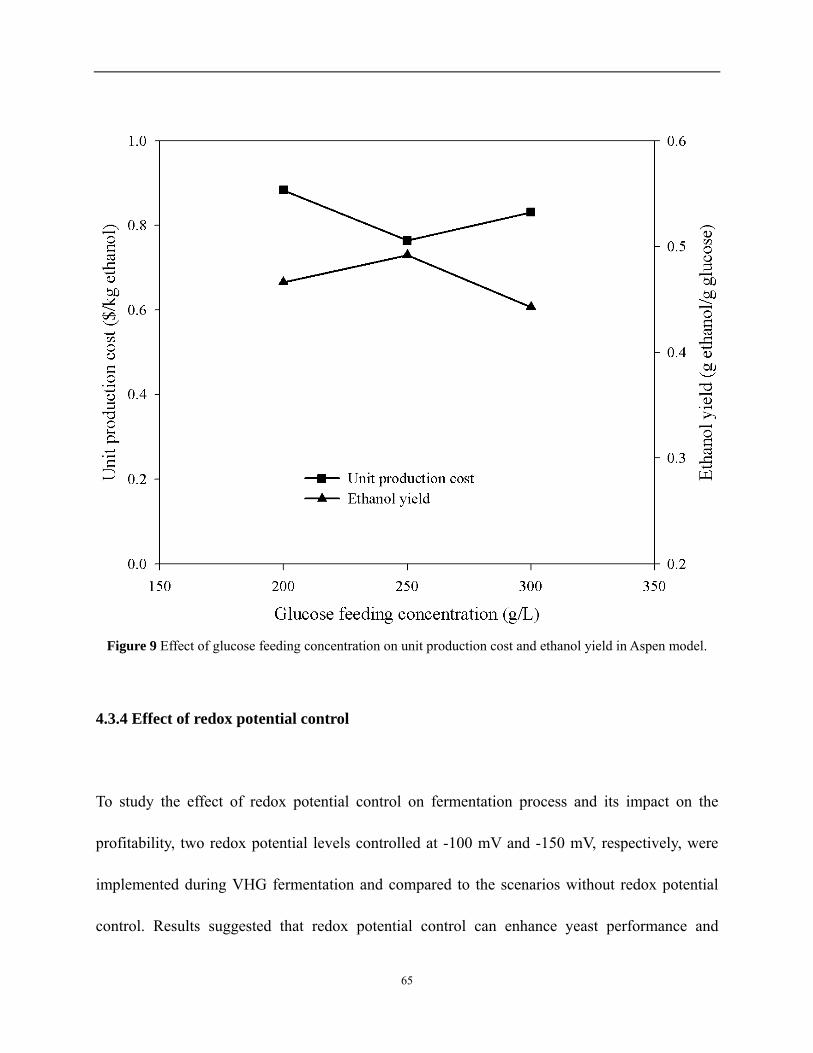
65
Figure 9 Effect of glucose feeding concentration on unit production cost and ethanol yield in Aspen model.
4.3.4 Effect of redox potential control
To study the effect of redox potential control on fermentation process and its impact on the
profitability, two redox potential levels controlled at -100 mV and -150 mV, respectively, were
implemented during VHG fermentation and compared to the scenarios without redox potential
control. Results suggested that redox potential control can enhance yeast performance and

66
improve fermentation efficiency, thus resulting in higher profit.
Effects of redox potential and glucose feeding concentration on the ethanol unit production cost
are shown in Figure 10. Under 300±6.42 g /L glucose feeding concentration, the unit production
cost of ethanol increased from 0.825 $/kg when no redox potential control was applied, to 0.888
$/kg when -100 mV redox potential was applied, and decreased dramatically to 0.780 $/kg when
redox potential was reduced from -100 mV to -150 mV. This result is also consistent with the
result shown in Figure 6a that ethanol yield increases from 0.4114 to 0.4677 when redox
potential was reduced from -100 mV to -150 mV. Applying an optimal redox potential control
level to the fermentation process may not only increase the ethanol yield in the fermenter thus
reduce the unit production cost, but also avoid procedural waste of raw material when VHG
fermentation process is applied for higher productivity and profitability.

67
Figure 10 Effect of redox potential control on ethanol unit production cost in Aspen model.

68
4.4 Comparison of Superpro and Aspen Plus models
4.4.1 Model basis
Brief illustrations of the Superpro model and Aspen Plus model were compared in Figure 11. As
mentioned before, because the software Superpro Designer used in the first process modeling has
a disadvantage that the number of equipment units is limited to be less than 25 in one process
model, therefore the liquefaction and saccharification sections of an ethanol producing were
ignored, as well as the treatment procedures of primary DDGS stream (centrifugation,
evaporation and drying).

69
Fermentor Distillation Molecular sieveGlucose
DDGS
Ethanol
Fermentor Distillation Molecular sieve
Saccharification
Liquefaction
Milling
Centrifugation
Evaporation
DryingCorn DDGS
Ethanol
Superpro model
Aspen Plus model Figure 11 Brief illustrations of the two models used for process simulation.
In the Superpro model, in order to approximate the product composition of the saccharification
section, glucose solution in certain concentrations with certain ingredients (protein, oil,
non-fermentable solids, non-starch polysaccharides), was directly used as the raw material feed
to the fermentor. On the other hand in the Aspen Plus model, corn (composed of starch, protein,
oil, non-starch polysaccharides, non-fermentable solids) was used as the raw material feed into
the whole process. Different feed stocks of the two models will predictably achieve different
results of economic evaluation, this will be discussed in section 4.4.3 “Model sensitivity to feed
stocks”.

70
In laboratory fermentation experiments, different redox potential controls were applied under
different initial glucose concentrations. However, in both of the two process simulators,
concentration of a certain component in the feed stream can not be simply defined as an input
parameter. In this occasion, mass composition of a certain component was used to precisely
manipulate the glucose concentration in feed of the fermentor. In general, mass composition of
glucose in the feed stream to fermentor was varied to achieve designed glucose concentration in
the very stream, while starch content in the feed stream to the milling procedure of the Aspen
Plus model was varied to achieve designed glucose concentration in the feed stream to fermentor.
In addition, because of the number limitation of equipment units used in the Superpro model,
many recycle streams used in a real ethanol plant to save raw materials and energy was also
ignored. Therefore, Aspen Plus was used to build a new model of an ethanol plant to overcome
the disadvantages of the Superpro model mentioned above, and another software Aspen Icarus
Process Evaluator was used for economical evaluation.
4.4.2 Equipment units
Equipment units used in two models are listed in Table 17. For the purpose of better
understanding of block type in the Aspen model, detailed description were presented in Table 18.
As shown in Figure 11, the Aspen Plus model is much more complicated hence a more accurate

71
model than the Superpro model to simulate the production process of a real ethanol fermentation
plant.

72
Table 17 Unit blocks used in both models. Superpro model (17 blocks) Aspen Plus model (37 blocks) Block Name Block Type Block Name Block Type PM-101 Centrifugal Pump AGETANK Flash2 C-101 Distillation Column BEERCOL RadFrac PM-102 Centrifugal Pump CENTRIF SSplit HX-103 Heat Exchanger CONDENSE Flash2 PM-103 Centrifugal Pump CTFSSPLT FSplit MX-102 Mixer DDGSDRYR Flash2 C-102 Distillation Column DEGAS Flash2 CSP-101 Component Splitter EVAP Flash2 PM-104 Centrifugal Pump FERMENT Rstoic PM-105 Centrifugal Pump H2OMIXER Mixer C-103 Distillation Column HEAT1 Heater V-103 Flat Bottom Tank HEAT2C Heater V-101 Fermentor HEAT2H Heater V-104 Blending Tank HEAT3 Heater GP-101 Gear Pump HEAT4C Heater AF-101 Air Filter HEAT4H Heater C-104 Absorber HEAT5 Heater HEAT6H Heater HEAT7C Heater HEAT7H Heater HEAT8 Heater HEAT9C Heater HEAT9H Heater HEAT10 Heater HEAT11 Heater HEAT12 Heater LIQUEFY Heater MILL Sep MIXCTF Mixer MIXDDGS Mixer MOLSIEVE Sep PCSPLIT FSplit PRESS Pump RECTIFY RadFrac SACCHAR Rstoic SCRUBBER RadFrac SEPETOH Sep

73
Table 18 Description of unit type in Aspen Plus model. Block type Category Description Flash2 Separators Two-outlet flash
RadFrac Columns Rigorous 2 or 3-phase fractionation
SSplit Mixers/Splitters Substream splitter
FSplit Mixers/Splitters Stream splitter
Rstoic Reactors Stoichiometric reactor based on known fractional conversions of extents of reactions
Mixer Mixers/Splitters Stream mixer
Heater Heat Exchangers Thermal and phase state changer
Sep Separators Component separator
Pump Pressure Changers Pump or hydraulic turbine
4.4.3 Model sensitivity to feed stocks
The influence of different feed stocks on unit production cost is shown in Table 19. The unit
production cost estimated by Superpro model is roughly twice of Aspen Plus’s estimated value
due to the great difference of feed stock purchasing price. However, even a huge gap exists
between the actual estimated values of the two models, a similar trend of these results was still
observed, as shown in Figure 12.
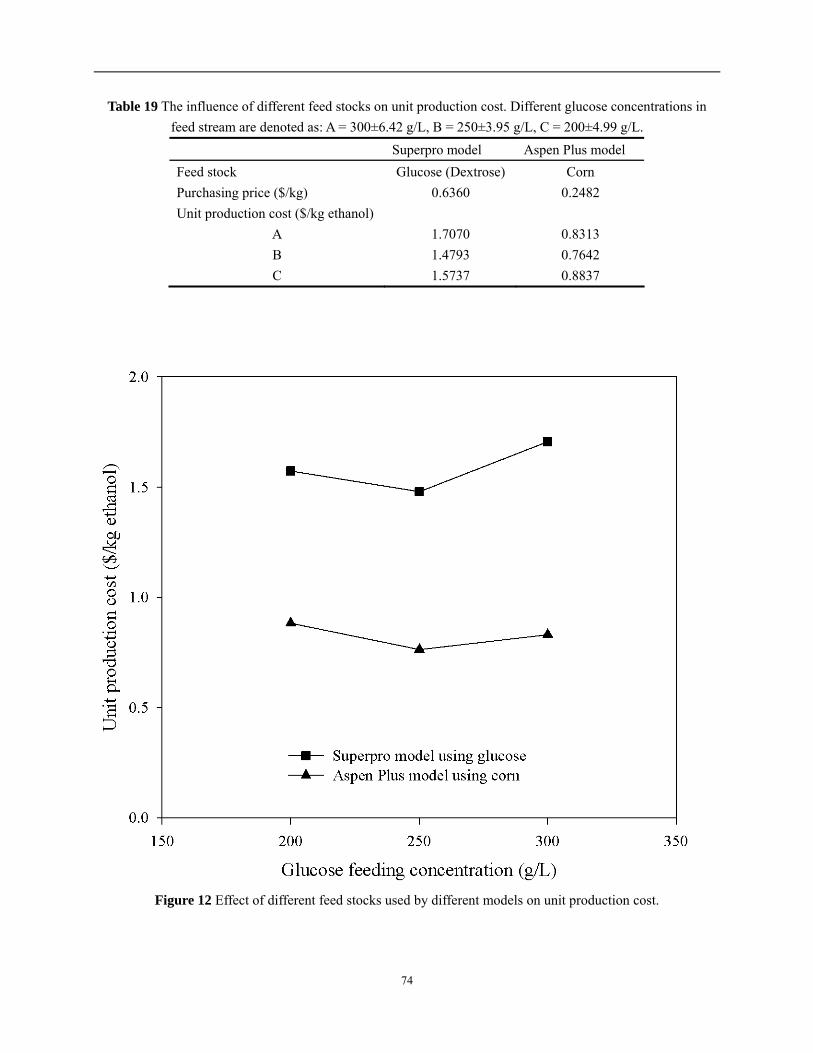
74
Table 19 The influence of different feed stocks on unit production cost. Different glucose concentrations in feed stream are denoted as: A = 300±6.42 g/L, B = 250±3.95 g/L, C = 200±4.99 g/L. Superpro model Aspen Plus model Feed stock Glucose (Dextrose) Corn Purchasing price ($/kg) 0.6360 0.2482 Unit production cost ($/kg ethanol)
A 1.7070 0.8313 B 1.4793 0.7642 C 1.5737 0.8837
Figure 12 Effect of different feed stocks used by different models on unit production cost.

75
As shown in Figure 12, the lowest unit production cost was achieved under 250±3.95 g/L feeding
glucose to fermentor, due to the highest ethanol yield (g ethanol/g glucose) under this condition.
Nevertheless, in the Superpro model, unit production cost estimated under 200±4.99 g/L glucose
feeding concentration is lower than the value under 300±6.42 g/L feeding glucose; while in the
Aspen Plus model this order went to the opposite way. This result might be caused by the
sensitivity difference of the two models to raw material cost, which accounts for roughly 90% of
the total unit production cost of ethanol, as shown in Table 20.
Table 20 Percentage of raw material cost in total unit production cost of two models. Different glucose concentrations in feed stream are denoted as: A = 300±6.42 g/L, B = 250±3.95 g/L, C = 200±4.99 g/L.
Different redox potential control levels are denoted as: a = no control, b = -150 mV, c = -100 mV. Superpro model Aspen Plus model
Scenario percentage
Condition average
Model average
Scenario percentage
Condition average
Model average
A a 91.10% 91.09% 89.92% 89.47% 89.48% 89.24% b 90.92% 89.41% c 91.25% 89.54%
B a 89.64% 89.77% 89.22% 89.23% b 89.89% 89.24% c 89.78% 89.22%
C a 88.94% 88.91% 89.02% 89.02% b 88.86% 89.01% c 88.93% 89.02%
It can be seen in Table 20 that even the percentages of raw material cost in total unit production
cost of two models are quite close, but variations of the condition averages which represent the
average value under different glucose feeding condition in the two models are relatively large.
Since the Superpro model has only 17 equipment units compared to 37 equipment units in the

76
Aspen Plus model as listed in Table 17, raw material cost will account for more share in the total
unit production cost. As a result, the Superpro model is more sensitive to variations of raw
material feed, especially when the feed is very high under VHG conditions. In addition, as
discussed above that low glucose feeding concentration (200±4.99 g/L) diminishes the efficiency
of the entire process, this diminishing effect is more considerable in the more complicated Aspen
Plus model than in the relatively simple Superpro model. Therefore, the highest unit production
cost was obtained under 300±6.42 g/L feeding glucose in the Superpro model, and under
200±4.99 g/L feeding glucose in the Aspen Plus model.
4.4.4 Product streams
Main properties of product streams (product purity) of the two models are compared in Table 21.
Due to the use of molecular sieves, purity of ethanol in the final product streams of both models
is quite close at over 99% of total mass.
Table 21 Comparison of product streams in the two models. Different glucose concentrations in feed stream are denoted as: A = 300±6.42 g/L, B = 250±3.95 g/L, C = 200±4.99 g/L.
Superpro model Aspen Plus model Product streams A B C A B C Main product
Ethanol (mass purity) 99.71% 99.68% 99.56% 99.34% 99.30% 99.37%
Byproduct DDGS (moisture content) 80.76% 86.79% 86.72% 31.65% 27.60% 28.82%
CO2 (mass purity) 74.46% 78.12% 79.09% 99.29% 99.31% 99.35%

77
On the other hand, the quality of byproduct streams is quite different from each other. According
to data from Agricultural Marketing Resource Center of ERS/USDA, 65~ 70% moisture in
DDGS stream (or called as Wet Distillers Grain) is allowed for the yield stream to be directly
sold as byproduct. Moisture content in the stream is usually controlled at 50~55% for Modified
Wet Distillers Grain, and 10% for Dried Distillers Grain. For this concern, DDGS yield from the
Superpro model needs further dehydration to be sold on market, while DDGS stream yield form
the Aspen Plus model can be directly sold on market as byproduct of ethanol fermentation
process.
For the CO2 stream produced from the Aspen Plus model, essentially all gas emission is CO2 and
no further processing is needed to recover CO2. But for the Superpro model, mass purity of CO2
produced from the process is not high enough for the stream to be directly sold as byproduct,
further treatment is still needed to remove nitrogen and oxygen in the stream.
4.4.5 Reaction accuracy
It should be noticed that even though the main reaction in the fermentor of both models
(Reaction 1 in the Superpro model and Reaction 5 in the Aspen Plus model) is almost the same,
and the same coefficients α, β are varied to apply laboratory fermentation results to both models,
the accuracy of these two coefficients in the two models is different. The coefficients in the
Aspen Plus model can be accurate to the fourth decimal place or more, while only second

78
decimal place accuracy is allowed in the Superpro model.
In Reaction 1 in the Superpro model (or Reaction 5 in the Aspen Plus model), the theoretical
value of α is 2, and thus 0 for β. However, under real fermentation conditions, certain amount of
biomass is produced from the substrate during fermentation, therefore α is always smaller than 2
in real conditions. Among all laboratory fermentation experiments, α is determined to range from
1.5775 to 1.9884 depending on glucose feeding concentrations and redox potential setting
applied to the fermentor.
For instance, in one fermentation experiments of which α is determined to be 1.7944, Reaction 4
in the Aspen Plus model will be defined as:
YDM 1234.0Ethanol 7944.1CO 7944.1Glucose 2 ++→
While Reaction 1 in the Superpro model can only be defined to be (β is dependent to α to ensure
mass balance of the equation, YDM in the Aspen model and Yeast Dry Matter in the Superpro
model are defined with different molecular weights):
MatterDry Yeast 05.1Alcohol Ethyl 79.1DioxideCarbon 79.1Glucose ++→
In this way, even exactly the same fermentation conditions were applied, the simulated ethanol
yield of the Superpro model is actually 2.45‰ lower than that of the Aspen Plus model. For a
plant with a capacity of 100 million kg ethanol/year, simply decrease in ethanol yield by 2.45‰
means reduction in Production rate by 245,000 kg ethanol/year, or loss of nearly 0.18 million
$/year in main product sales.

79
Under large scale productions, even the smallest variations of the reactions defined in the
fermentor may eventually cause huge difference of the final evaluation results. The Aspen Plus
model obviously achieves better accuracy on process simulation than the Superpro model.

80
4.5 Disposal of CO2 produced during fermentation
During the fermentation process which yeast cells convert glucose to ethanol, equal number of
carbon dioxide molecules will be produced. For a plant with a capacity of 100 million kg/year of
ethanol, 95.53 million kg/year of carbon dioxide will also be produced. Three options for the
disposal of CO2 were presented in Figure 13.
CO2 produced during fermentation
Emission into atmosphere
Captured and sold as coproduct
Deep injection into geological
formations for storage
Figure 13 Options for disposal of CO2 during bio-ethanol fermentation.
Most fermentation facilities emit their CO2 to the atmosphere. This is not only a waste of
resource, but more importantly not environmental preferable since CO2 is one of the major
greenhouse gases that causing global warming problem. In some facilities, CO2 is assumed to be
sold for carbonate beverages or dry ice production. Selling CO2 as a byproduct of fermentation
process has no significant impact on reducing the production cost of ethanol (Wingren et al.,
2003), but is still profitable for facilities with large CO2 production rate, and is environmental

81
friendly.
For a fermentation process like the studied one, essentially all gas emissions is CO2 and no
further processing is needed to recover CO2 (Möllersten and Moreira, 2003). The selling price of
industrial level CO2 is estimated to be 15.94 $/ton (Wingren et al., 2003), then for the process
with a capacity of 100 million kg ethanol/year, selling CO2 as a byproduct will bring in 1.52
million $/year as extra income. Selling CO2 as a byproduct is profitable, however, it is still
questionable whether this could be actually implemented if many ethanol plants were established,
because the market for CO2 could become saturated to consume such large amount of CO2.
In fact, there are growing commercial-scale experiences that CO2 is injected into deep
underground geological formations to avoid leakage into atmosphere (Bachu et al., 2003). The
experience of acid-gas injection operations showed that CO2 sequestration in geological media is
a mature and safe technology that can successfully be expanded to and applied in large-scale
operations that will reduce CO2 emissions into the atmosphere from large CO2 point sources
(Kheshgi and Prince, 2005). For the scenario mentioned above, the CO2 production rate is
assumed to be 95.53 million kg/year, and the plant locates 500 km away from the deep injection
site, therefore the capture cost is estimated to be 50 $/ton CO2 including capture and
transportation (Möllersten and Moreira, 2003), so the CO2 deep injection cost for the plant will
be 4.78 million $/year. Shorter transportation distance and larger Production rate further reduces
the unit cost of CO2 storage and transportation, evaluation parameters can be obtained from

82
McCoy (2008) and (Möllersten and Moreira, 2003) for different scenarios.
Furthermore, if fermentation CO2 can be stored (e.g. in a geological reservoir), some of the CO2
taken up during crop growth would not be released back to the atmosphere but sequestered
underground. If this exceeded the fossil carbon emitted during ethanol production, then the
production of ethanol would result in the net removal of CO2 from the atmosphere. Note the deep
injection operations for carbon sequestration are also applicable to many other sites around the
world (Thambimuthu, 2004).
The compression and transport of CO2 to the sequestration site would add cost (Kheshgi and
Prince, 2005). McCoy (2008) gave some methods to estimate the pipeline cost for large amount
CO2 transportation based on different flow rates and distances. However, in North America, such
acid-gas deep injection operations were already started since 1989 (Bachu et al., 2003). Using
existed pipelines to transport CO2 to sequestration sites or building CO2 generating sources such
bio-ethanol fermentation plants near deep injection sites will lower the cost of deep injection.

83
CHAPTER 5 CONCLUSIONS AND RECOMMENDATIONS
5.1 Conclusions
In this study, Superpro Designer as one of the process simulators was mainly used to explore the
effects of applied glucose feeding concentrations and redox potential control settings on process
economics, since the Superpro model is not a complete process for ethanol fermentation, results
of economical evaluation were only used to compare to each other to study effects of different
applied conditions on fermentation, thus not appropriate for reference on market. On the other
hand, results from Aspen utilities (Aspen Plus as the simulator, Aspen IPE as the evaluator) are
quotable to be compared with real market prices.
According to simulated results, VHG condition of 300±6.42 g/L glucose feeding concentration
did not achieve the expected reduction on unit production rate of ethanol. The results suggested
that the most profitable glucose feeding concentration to the fermenter is around 250±3.95 g/L
among all studied scenarios, which gives the lowest ethanol unit production cost and shortest
process payout period, with or without redox potential control. Application of VHG fermentation
process requires not only an industrial yeast strain to efficiently utilize fermentable substrates
within shorter residence time, but also approaches to reuse residual saccharides in the output
stream of the fermentor.
84
Redox potential control has certain effects on fermentation process, especially for VHG
fermentation process. Results suggest that controlling redox potential level at -150 mV during
fermentation increases the ethanol yield, therefore considerably reduces the unit production cost
under VHG conditions. However, the optimal combination of redox potential control level and
glucose feeding concentration requires further examination.
Since large amount of CO2 is produced during fermentation process, to capture and sell CO2 is
profitable for plants with large capacity despite the extra costs of a CO2 recovery system. In
addition, CO2 is known as the major greenhouse gas which causes global warming. Despite that
the deep injection alternative for disposal of CO2 produced during fermentation is not
economically preferable comparing to whether emitting CO2 to atmosphere or selling it as a
byproduct, the deep injection operation to reduce CO2 emission to atmosphere is currently much
more environmental friendly, and is of great long term benefits.

85
5.2 Recommendations
As discussed above, redox potential setting has different effects on ethanol yield (substrate
utilization rate) according to different initial glucose concentrations of fermentation. In
laboratory experiments, only two redox potential settings, -100 mV and -150 mV, were
compared to no redox potential control conditions to study its effect on fermentation process. In
future studies, more redox potential setting levels might need to be applied to determine the
optimum value for the highest ethanol yield. Besides, these redox potential controlled
fermentation experiments were carried out in lab scale, therefore further and more specific tests
are required for industrial scale fermentation.

86
REFERENCES
Bachu, S., J. J. Adams, K. Michael, and B. E. Buschkuehle, “Acid gas injection in the Alberta Basin: a commercial-scale analogue for CO2 geological sequestration in sedimentary basins,” Second annual conference on carbon sequestration, Washington.D.C, National Energy Technology Laboratory, United States Department of Energy (2003).
Casey, G.P., C.A. Magnus, and W.M. Ingledew, “High-Gravity Brewing: Effects of Nutrition on
Yeast Composition, Fermentative Ability, and Alcohol Production,” Applied and Environmental Microbiology, 639 (1984).
Duncan, M., “U. S. Federal Initiatives to Support Biomass Research and Development,” Journal
of Industrial Ecology, 7(3-4), 193(2003). Eidman, V.R., “Renewable Liquid Fuels: Current Situation and Prospects,” Choices 21(1),
15(2006). EthanolIndia, http://www.ethanolindia.net/molecular_sieves.html, August 1, 2011. Gibreel A., J.R. Sandercock, J. Lan, L.A. Goonewardene, R.T. Zijlstra, J.M. Curtis, and D.C.
Bressler, “Fermentation of barley by using Saccharomyces cerevisiae: Examination of barley as a feedstock for bioethanol production and value-added products”, Applied and Environmental Microbiology, 75, 1363 (2009).
Kheshgi, H. S. and R. C. Prince, “Sequestration of fermentation CO2 from ethanol production,”
Energy, 30, 1865 (2005). Ko, J., W. J. Su, I. L. Chien, D. M. Chang, S. H. Chou, and R. Y. Zhan, “Dynamic modeling and
analyses of simultaneous saccharification and fermentation process to produce bio-ethanol from rice straw,” Bioprocess and Biosystems Engineering, 22, 195 (2010).
Kwiatkowski, J. R., A. J. McAloon, F. Taylor, and D. B. Johnston, “Modeling the process and
costs of fuel ethanol production by the corn dry-grind process,” Industrial Crops and Products, 23, 288 (2006).
Lin, Y.H., W. Chien, and K. Duan, “Correlation between reduction-oxidation potential profiles
and growth patterns of Saccharomyces cerevisiae during very-high-gravity fermentation,” Process Biochemistry, 45, 765 (2010).
87
McCoy, S.T. “The economics of CO2 transport by pipeline and storage in saline aquifers and oil resevoirs,” Ph.D. Thesis, Department of Engineering and Public Policy, Carnegie Mellon University, Pittsburgh, PA, USA (2008).
Möllersten, K., J. Yan, and J. R. Moreira, “Potential market niches for biomass energy with CO2
capture and storage-opportunities for energy supply with negative CO2 emissions,” Biomass and Bioenergy, 25, 273 (2003).
Nevoigt, E., “Progress in metabolic engineering of Saccharomyces cerevisiae,” Microbiology
and Molecular Biology Reviews, 72, 379 (2008). Nghiem, N.P., K.B. Hicks, D.B. Johnston, G. Senske, M. Kurantz, M. Li, J. Shetty and G
Konieczny-Janda, “Production of ethanol from winter barley by the EDGE (enhanced dry grind enzymatic) process,” Biotechnology for Biofuels, 3, 8 (2010).
Ochoa, S., A. Yoo, J. U. Repke, G. Wozny, and D. R. Yang, “Modeling and parameter
identification of the simultaneous saccharification-fermentation process for ethanol production,” Biotechnology Progress, 23, 1454 (2007).
Pratt, P.L., J.H. Bryce, and G.G. Stewart, “The effects of osmotic pressure and ethanol on yeast
viability and morphology,” Journal of the Institute of Brewing, 109, 218 (2003). Rajagopalan,S., E. Ponnampalam, D. McCalla, and M. Stowers, “Enhancing profitability of dry
mill ethanol plants,” Applied Biochemistry and Biotechnology, 120, 37 (2005). Ramirez, E. C., D. B. Johnson, A. J. McAloon, and V. Singh, “Enzymatic corn wet milling:
Engineering process and cost model,” Biotechnology for Biofuels, 2, 2 (2009). Sainz, J., F. Pizarro, J. R. Pérez-Correa, and E. Agosin, “Modeling of yeast metabolism and
process dynamics in batch fermentation,” Biotechnology and Bioengineering, 81, 818 (2003). Taylor, F., M. J. Kurantz, N. Goldberg, A. J. McAloon, and J.C. Craig.Jr., “Dry-Grind Process for
Fuel Ethanol by Continuous Fermentation and Stripping,” Biotechnology Progress,16, 541 (2000).
Thambimuthu, K., 2010, “IEA Weyburn CO2 Monitoring and Storage Project,” IEA Greenhouse
Gas R&D Programme. http://www.iea.org/work/2004/zets/conference/presentations/thambimuthu.pdf (2004).
Thomas, K. C. and W. M. Ingledew, “Fuel alcohol production: Effects of free amino nitrogen on
fermentation of very-high-gravity wheat mashes,” Applied and Environmental Microbiology,

88
56, 2046 (1990). Thomas, K.C., S.H. Hynes, A.M. Jones, and W.M. Ingledew, “Production of fuel alcohol from
wheat by VHG technology: effect of sugar concentration and fermentation temperature,” Applied Biochemistry and Biotechnology, 43, 211 (1993).
Wingren, A., M. Galbe, and G. Zacchi, “Techno-economic evaluation of producing ethanol from
softwood: comparison of SSF and SHF and identification of bottlenecks,” Biotechnology Progress, 19, 1109 (2003).
Yang, D.M. “Gene expression profiling in Saccharomyces cerevisiae grown at different specific
gravity environments,” M.Sc. Thesis, Department of Chemical Engineering, University of Saskatchewan, Saskatoon, SK, Canada (2007).
Zhang, C., W. Han, X. Jing, G. Pu, and C. Wang, “Life cycle economic analysis of fuel ethanol
derived from cassava in southwest China,” Renewable and Sustainable Energy Reviews, 7(4), 353 (2003).
Zhao, Y., and Y.H. Lin, “Growth of Saccharomyces cerevisiae in a chemostat under high glucose
conditions,” Biotechnology Letters, 25, 1151 (2003).

89
APPENDICES Appendix A – Experimental data used for process simulation
Table A Experimental data used for process simulation. In the first column of scenarios, different glucose concentrations in feed stream are denoted as: A = 300±6.42 g/L, B = 250±3.95 g/L, C = 200±4.99 g/L.
Different redox potential control levels are denoted as: a = no control, b = -150 mV, c = -100 mV. 1 and 2 stand for different repeats of an individual scenario.
Conditions Fermentation temperature (℃)
Aeration rate (VVM)
Fermentation time (hours)
Initial glucose concentration (g/L)
Final glucose concentration (g/L)
Final ethanol concentration (g/L)
Aa1 30 0 48 302.15 15.37 125.950Aa2 30 0 48 294.69 20.57 125.940Ab1 30 0.0023741 48 313.05 20.35 134.305Ab2 30 0.0023741 48 299.31 4.71 140.384Ac1 30 0.0076624 48 300.66 23.26 116.347Ac2 30 0.0076624 48 303.62 2.08 121.639Ba1 30 0 42 256.44 0 130.390Ba2 30 0 42 246.84 0 119.614Bb1 30 0.0003083 36 254.11 0 122.855Bb2 30 0.0003083 36 251.52 0 121.595Bc1 30 0.0020317 36 256.89 0 126.140Bc2 30 0.0020317 36 254.97 0 127.715Ca1 30 0 24 200.93 0 93.740Ca2 30 0 24 202.18 0 94.025Cb1 30 0.0003912 24 199.08 0 95.640Cb2 30 0.0003912 24 202.93 0 94.040Cc1 30 0.0254238 24 212.49 0 96.085Cc2 30 0.0254238 24 205.71 0 96.785
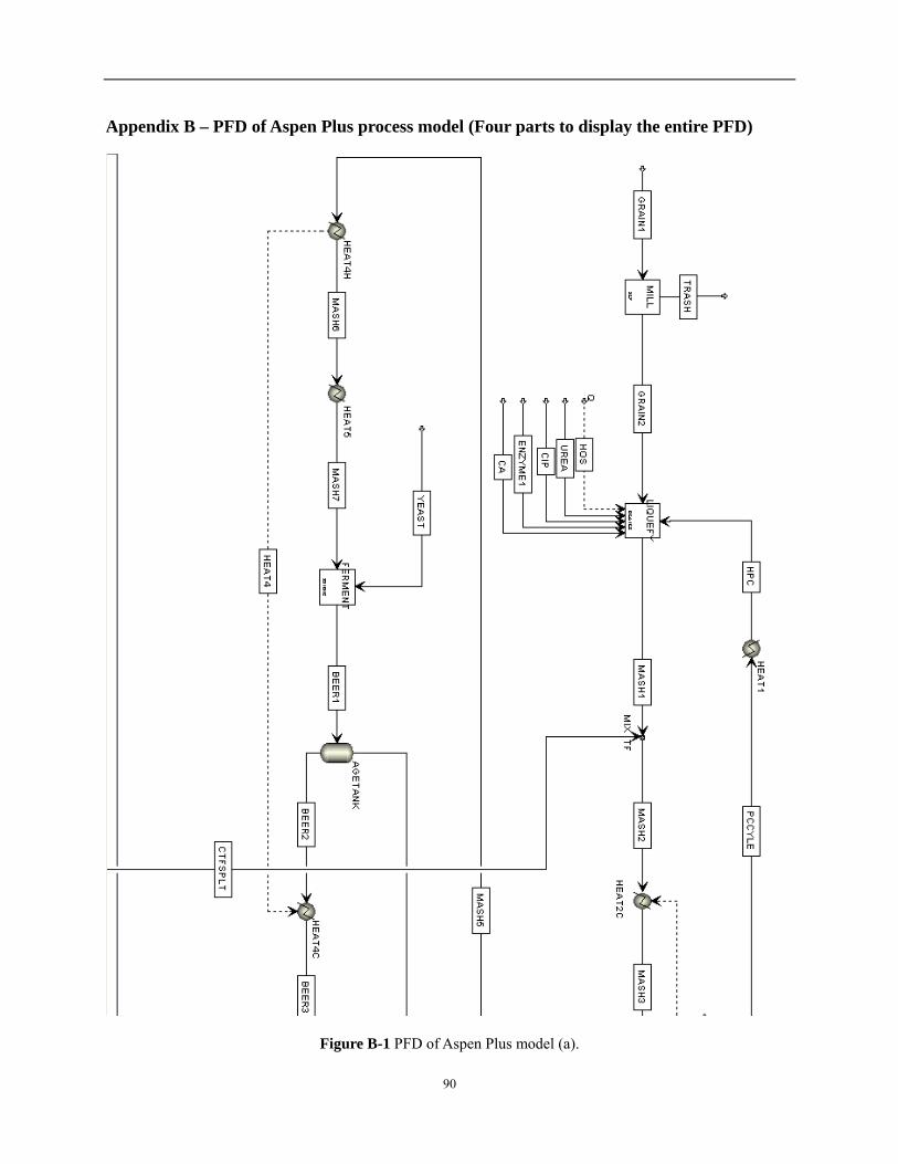
90
Appendix B – PFD of Aspen Plus process model (Four parts to display the entire PFD)
Figure B-1 PFD of Aspen Plus model (a).

91
Figure B-2 PFD of Aspen Plus model (b).

92
Figure B-3 PFD of Aspen Plus model (c).

93
Figure B-4 PFD of Aspen Plus model (d).
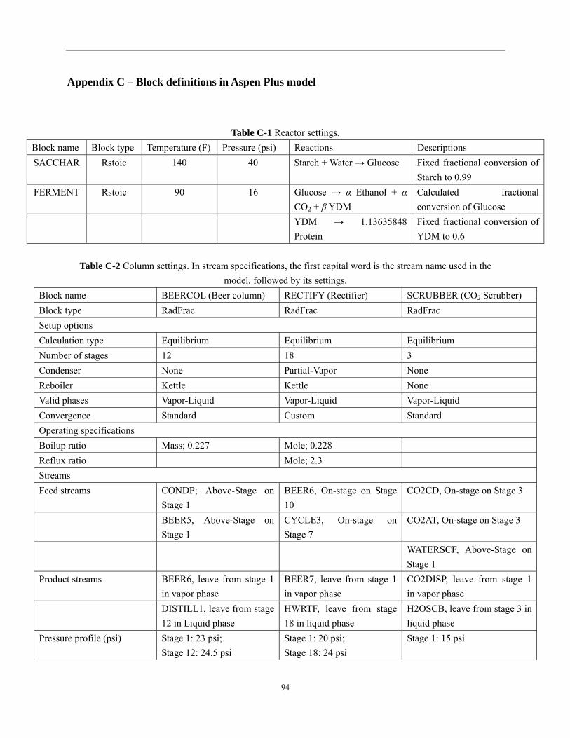
94
Appendix C – Block definitions in Aspen Plus model
Table C-1 Reactor settings. Block name Block type Temperature (F) Pressure (psi) Reactions Descriptions SACCHAR Rstoic 140 40 Starch + Water → Glucose Fixed fractional conversion of
Starch to 0.99 FERMENT Rstoic 90 16 Glucose → α Ethanol + α
CO2 + β YDM Calculated fractional conversion of Glucose
YDM → 1.13635848 Protein
Fixed fractional conversion of YDM to 0.6
Table C-2 Column settings. In stream specifications, the first capital word is the stream name used in the
model, followed by its settings. Block name BEERCOL (Beer column) RECTIFY (Rectifier) SCRUBBER (CO2 Scrubber) Block type RadFrac RadFrac RadFrac Setup options Calculation type Equilibrium Equilibrium Equilibrium Number of stages 12 18 3 Condenser None Partial-Vapor None Reboiler Kettle Kettle None Valid phases Vapor-Liquid Vapor-Liquid Vapor-Liquid Convergence Standard Custom Standard Operating specifications Boilup ratio Mass; 0.227 Mole; 0.228 Reflux ratio Mole; 2.3 Streams Feed streams CONDP; Above-Stage on
Stage 1 BEER6, On-stage on Stage 10
CO2CD, On-stage on Stage 3
BEER5, Above-Stage on Stage 1
CYCLE3, On-stage on Stage 7
CO2AT, On-stage on Stage 3
WATERSCF, Above-Stage on Stage 1
Product streams BEER6, leave from stage 1 in vapor phase
BEER7, leave from stage 1 in vapor phase
CO2DISP, leave from stage 1 in vapor phase
DISTILL1, leave from stage 12 in Liquid phase
HWRTF, leave from stage 18 in liquid phase
H2OSCB, leave from stage 3 in liquid phase
Pressure profile (psi) Stage 1: 23 psi; Stage 12: 24.5 psi
Stage 1: 20 psi; Stage 18: 24 psi
Stage 1: 15 psi

95
Condenser Subcooling specification Subcooled temperature at
175 F, only reflux is subcooled
Design specs 0.0005 mass purity of component Ethanol in product stream DISTILL1
0.9085 mass purity of component Ethanol in vapor of Stage 1 as internal stream
0.0005 mass purity of component Ethanol in total liquid of Stage 18 as internal stream
Vary Boilup ratio from 0.15 to 1 Reflux ratio from 1 to 5 Boilup ratio from 0.01 to 1 Tray sizing Starting stage 1 2 Ending stage 11 10 Tray type Sieve Sieve Number of passes 1 1 Tray spacing (m) 0.6096 0.6096 Fractional approach to flooding
0.6175 0.6175
Starting stage 11 Ending stage 17 Tray type Sieve Number of passes 1 Tray spacing (m) 0.6096 Fractional approach to flooding
0.5
Flooding calculation method
Fair
Pack sizing Starting stage 1 Ending stage 3 Type SUPER-INTX Vendor NORTON Material CERAMIC Dimension 1-IN OR 25-MM Height equivalent to a theoretical plate (ft)
5

96
Table C-3 Flash settings. Block name Block type Temperature (F) Pressure (psi) Maximum
iterations Error tolerance
AGETANK Flash2 90 16 30 1E -06 CONDENSE Flash2 100 16 30 1E -06
DDGSDRYR Flash2 220 14.7 30 1E -05
DEGAS Flash2 184 30 1E -04
EVAP Flash2 202.8 Vapor fraction: 0.88588 30 1E -06
Table C-4 Heater settings. Block name Block type Temperature (F) Pressure (psi) Maximum
iterations Error tolerance
HEAT1 Heater 110 50 30 1E -05 HEAT2C Heater 50 30 1E -05 HEAT2H Heater 208 50 30 1E -05 HEAT3 Heater 230 50 30 1E -05 HEAT4C Heater 30 30 1E -04 HEAT4H Heater 112 40 30 1E -06 HEAT5 Heater 90 40 30 1E -06 HEAT6H Heater 140 50 30 1E -05 HEAT7C Heater 50 30 1E -04 HEAT7H Heater 200 40 30 1E -05 HEAT8 Heater 240 19.75 30 1E -05 HEAT9C Heater 22.5 30 1E -06 HEAT9H Heater 184.17 14.8 30 1E -04 HEAT10 Heater 95 22 30 1E -04 HEAT11 Heater 68 18.5 30 1E -05 HEAT12 Heater 131.5 15 30 1E -05 LIQUEFY Heater 50 30 1E -04
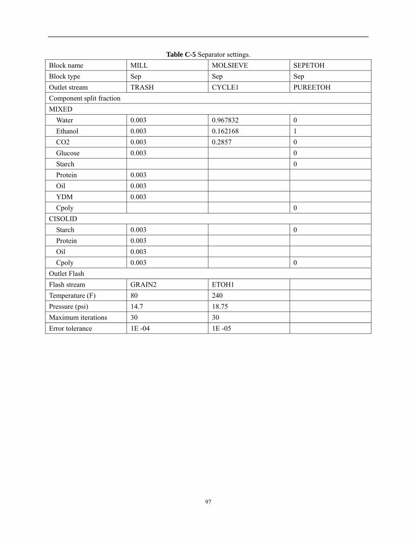
97
Table C-5 Separator settings. Block name MILL MOLSIEVE SEPETOH Block type Sep Sep Sep Outlet stream TRASH CYCLE1 PUREETOH Component split fraction MIXED Water 0.003 0.967832 0 Ethanol 0.003 0.162168 1 CO2 0.003 0.2857 0 Glucose 0.003 0 Starch 0 Protein 0.003 Oil 0.003 YDM 0.003 Cpoly 0 CISOLID Starch 0.003 0 Protein 0.003 Oil 0.003 Cpoly 0.003 0 Outlet Flash Flash stream GRAIN2 ETOH1 Temperature (F) 80 240 Pressure (psi) 14.7 18.75 Maximum iterations 30 30 Error tolerance 1E -04 1E -05
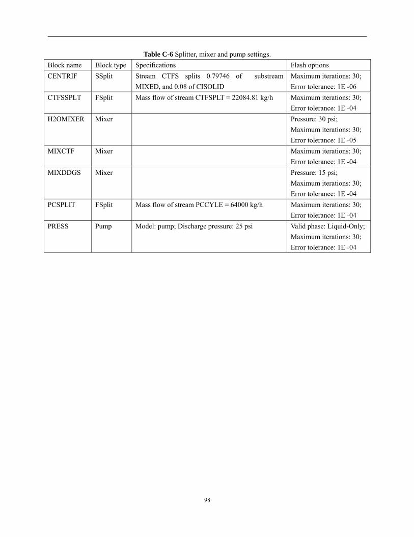
98
Table C-6 Splitter, mixer and pump settings. Block name Block type Specifications Flash options CENTRIF SSplit Stream CTFS splits 0.79746 of substream
MIXED, and 0.08 of CISOLID Maximum iterations: 30; Error tolerance: 1E -06
CTFSSPLT FSplit Mass flow of stream CTFSPLT = 22084.81 kg/h Maximum iterations: 30; Error tolerance: 1E -04
H2OMIXER Mixer Pressure: 30 psi; Maximum iterations: 30; Error tolerance: 1E -05
MIXCTF Mixer Maximum iterations: 30; Error tolerance: 1E -04
MIXDDGS Mixer Pressure: 15 psi; Maximum iterations: 30; Error tolerance: 1E -04
PCSPLIT FSplit Mass flow of stream PCCYLE = 64000 kg/h Maximum iterations: 30; Error tolerance: 1E -04
PRESS Pump Model: pump; Discharge pressure: 25 psi Valid phase: Liquid-Only;Maximum iterations: 30; Error tolerance: 1E -04

99
Appendix D – Glossary
Abstract Capacity: Capacity of plant for major product Payout period: Payout Period is the expected number of years required to recover the original investment in the project. This parameter indicates the length of time that the facility needs to operate in order to recover the initial capital investment (total capital cost plus working capital). Redox potential: Redox (shorthand for reduction–oxidation) potential (a.k.a. oxidoreduction potential, ORP) quantifies the momentary status of a biological activity, either oxidized or reduced. During fermentation, the major contributors to the changes of redox potential are NADH (served as electron donor) due to assimilatory processes such as biomass formation and dissimilatory processes such as glycolysis, and dissolved oxygen (served as electron acceptor) resulting from agitation and/or sparging. The changes of redox potential are thus related to the extent of intracellular activities to the amount of extracellular dissolved oxygen level. Unit production cost: Is the cost associated with production divided by the number of units produced. Unit costs include all fixed costs (i.e. plant and equipment) and all variable costs (labor, materials, etc.) involved in production. Very high gravity fermentation: Or short for VHG fermentation, fermentation with initial glucose concentration greater than 250 g/L.
Chapter 1 Liquefaction: Also known as starch liquefaction. The production of beverage alcohol from floury raw materials requires in the first place the digestion of starch by thermal pretreatment and subsequent starch liquefaction, involving the partial hydrolysis of the starch, with concomitant loss in viscosity. Saccharification: The process of converting complex carbohydrate (e.g. starch) into simple monosaccharide components (e.g. glucose) through hydrolysis. In the production of potable distilled alcohol, the digested, liquefied starch is enzymatically split into fermentable sugar. Saccharomyces cerevisiae: Is a species of yeast that is widely used in brewing beer. It is perhaps the most useful yeast, having been instrumental to baking and brewing since ancient times. Also called as brewer’s yeast, baker’s yeast, budding yeast or top-fermenting yeast. Unit procedure: A unit procedure is defined as a series of operations that take place within a

100
piece of equipment. The types of operations available depend on the type of unit procedure you are using.
Chapter 2 Ambient temperature: Ambient temperature is a term which refers to the temperature in a room, or the temperature which surrounds an object under discussion. Azeotrope: An azeotrope is a mixture of two or more liquids in such a ratio that its composition cannot be changed by simple distillation. This occurs because, when an azeotrope is boiled, the resulting vapor has the same ratio of constituents as the original mixture. Because their composition is unchanged by distillation, azeotropes are also called (especially in older texts) constant boiling mixtures. Azeotropic distillation: In chemistry, azeotropic distillation is any of a range of techniques used to break an azeotrope in distillation. In chemical engineering, azeotropic distillation usually refers to the specific technique of adding another component to generate a new, lower-boiling azeotrope that is heterogeneous (e.g. producing two, immiscible liquid phases). Bio-ethanol: Biologically produced ethanol, produced by the action of microorganisms and enzymes through the fermentation of sugars or starches (easiest), or cellulose (more difficult). Latent heat of vaporization: The heat absorbed when a substance changes phase from liquid to gas. Molecular sieve: A molecular sieve is a material containing tiny pores of a precise and uniform size that is used as an adsorbent for gases and liquids. Molecules small enough to pass through the pores are adsorbed while larger molecules are not. Molecular sieves are often utilized in the petroleum industry, especially for the purification of gas streams and in the chemistry laboratory for separating compounds and drying reaction starting materials. Super heater: A superheater is a device used to convert saturated steam or wet steam into dry steam used for power generation or processes. There are three types of superheaters namely: radiant, convection, and separately fired. A superheater can vary in size from a few tens of feet to several hundred feet. Unslaked lime: Calcium oxide (CaO), commonly known as quicklime or burnt lime, is a widely used chemical compound. It is a white, caustic, alkaline crystalline solid at room temperature.
Chapter 3

101
Annual operating cost: The total of raw material, operating labor, maintenance, operating charges, plant overhead and G and A expenses per year. Annual production rate: the production rate (usually the main product) on a year base. Conversion factor: factor for adequate liquid distribution & irrigation across the scrubber bed. Countercurrent: refer to countercurrent exchange, is a mechanism occurring in nature and mimicked in industry and engineering, in which there is an almost total crossover of some property between two flowing bodies. The flowing bodies can be liquids, gases, plasma, or even solid powders, or any combination of those. Critical surface tension: The critical surface tension of a solid surface is an indication of its relative water-hating or water-loving character. A low critical surface tension means that the surface has a low energy per unit area. The quantity is based on experiments with a series of pure liquids. Diffusivity: Diffusivity or diffusion coefficient is a proportionality constant between the molar flux due to molecular diffusion and the gradient in the concentration of the species (or the driving force for diffusion). Facility type: Defines the facility type. The following types are currently available: Chemical Processing Facility, Food Processing Facility, Oil Refining Facility, Petrochemical Processing Facility, Pharmaceutical Facility, Pulp and/or Paper Processing Facility, Specialty Chemical Processing Facility (A specialty chemical is defined as a chemical which is produced in low quantity and has a usually high price per unit.). The type of facility affects the number of operators/shift and maintenance costs of facility equipment. G and A Expenses: represents general and administrative costs incurred during production such as administrative salaries/expenses, R&D, product distribution and sales costs. Specify this number as a percentage of subtotal operating costs. Heat transfer coefficient: The heat transfer coefficient, in thermodynamics and in mechanical and chemical engineering, is used in calculating the heat transfer, typically by convection or phase change between a fluid and a solid. Heat transfer coefficient is the proportionality coefficient between the heat flux that is a heat flow per unit area, q/A, and the thermodynamic driving force for the flow of heat (i.e., the temperature difference, ΔT). HPLC: High-performance liquid chromatography (sometimes referred to as high-pressure liquid chromatography), HPLC, is a chromatographic technique that can separate a mixture of compounds and is used in biochemistry and analytical chemistry to identify, quantify and purify

102
the individual components of the mixture. HPLC typically utilizes different types of stationary phases, a pump that moves the mobile phase(s) and analyte through the column, and a detector to provide a characteristic retention time for the analyte. Installation cost: The factor is used to estimate installation cost for each piece of equipment by directly multiplying the purchase cost of the equipment. Intermediate product: Product that has undergone a partial processing and is used as raw material in a successive productive step. Laboratory Charges: Is a cost per period indicating the cost of having product analyzed each period. Length of Start-up Period: After the facility has been constructed (i.e., gone through engineering, procurement and construction), the plant must go through the owner’s start-up period until it starts producing the product to be sold. This period is referred to as Length of Start-up Period in weeks and is added into the EPC duration. Material factor: The purchase cost as calculated by the options set by the purchase cost, estimates the cost of equipment assuming a reference material of construction. For all other materials, the purchase cost is adjusted by multiplying with a material-specific factor. The list of eligible materials for every equipment type and the corresponding material factors can be found in the Superpro databank. Nominal diameter: The diameter computed for a hypothetical sphere which would have the same volume as the calculated volume for a specific sedimentary particle, also known as equivalent diameter. NPV interest: The net present value (NPV) is a profitability measure used to evaluate the viability of an investment or to compare the profitability of a number of different investments. It represents the total value of future net cash flows during the life time of a project, discounted to reflect the time value of money at the beginning of a project (i.e., at time zero). It is calculated for three different interest rates (low, medium and high). Operating and Maintenance Labor Escalation: is the rate at which the operating and maintenance costs of the facility are to be escalated (increased) in terms of percent per period. The operating labor costs include operators per shift and supervisory costs. Operating Charges: Includes operating supplies and laboratory charges. It is specified as a percentage of the operating labor costs.

103
Operating Hours per Period: Refers to the number of hours per period that the plant will be operating. Operating mode: Refers to the operating mode of the facility. The available options are: Continuous Processing - 24 Hours/Day, Continuous Processing - Less than 24 Hours/Day, Batch Processing - 24 Hours/Day, Batch Processing - 1 Batch per Shift, Batch Processing - More than 1 Batch per Shift, Intermittent Processing - 24 Hours/Day, Intermittent Processing - Less than 24 Hours/Day. The operating mode of the facility affects the number of operators/shift and maintenance costs of facility equipment. Operating Supplies: Indicates the cost of miscellaneous items that are required in order to run the plant in terms of cost per period. PID Controller: A proportional–integral–derivative controller (PID controller) is a generic control loop feedback mechanism (controller) widely used in industrial control systems – a PID is the most commonly used feedback controller. A PID controller calculates an "error" value as the difference between a measured process variable and a desired set point. The controller attempts to minimize the error by adjusting the process control inputs. Plant Overhead: consists of charges during production for services, facilities, payroll overhead, etc. This number is specified as a percent of operating labor and maintenance costs. This number should not be used for the construction of the facility, only for operation after start-up. Process Fluids: Indicate the types of fluids involved in the process. The selection affects operating and maintenance costs. The selections are: Liquids, Liquids and Gases, Liquids and Solids, Liquids, Gases, and Solids, Gases, Gases and Solids, Solids. Product sales: Total product sales per period. This number is generated by multiplying Products Sales per Hour by Operating Hours per Period. Products Escalation: Is the rate at which the sales revenue from products of the facility is to be escalated (increased) in terms of percent per period. Project Capital Escalation: Indicates the rate at which project capital expenses may increase expressed in percent per period. If the addition of Engineer-Procure-Construct (EPC) period and start-up period is greater than one whole period, Project Capital Escalation is used to escalate the capital expenses for periods beyond the first period. Pump efficiency: Pump efficiency is defined as the ratio of the power imparted on the fluid by the pump in relation to the power supplied to drive the pump. Its value is not fixed for a given pump, efficiency is a function of the discharge and therefore also operating head.

104
Raw Material Escalation: is the rate at which the raw material costs of the facility are to be escalated (increased) in terms of percent per period. Reaction extent: The extent of reaction can be regarded as a real (or hypothetical) product, one molecule of which is produced each time the reaction event occurs. It is the extensive quantity describing the progress of a chemical reaction equal to the number of chemical transformations, as indicated by the reaction equation on a molecular scale, divided by the Avogadro constant Revenue stream: A revenue stream is any stream that generates income. Typically, a revenue stream is an output stream that can be sold. Sometimes revenue streams are also called product streams. There may be several revenue (or product) output streams in a process. RI detector: The refractive index (RI) detector is the only universal detector in HPLC. The detection principle involves measuring of the change in refractive index of the column effluent passing through the flow-cell. The greater the RI difference between sample and mobile phase, the larger the imbalance will become. Thus, the sensitivity will be higher for the higher difference in RI between sample and mobile phase. On the other hand, in complex mixtures, sample components may cover a wide range of refractive index values and some may closely match that of the mobile phase, becoming invisible to the detector. RI detector is a pure differential instrument, and any changes in the eluent composition require the rebalancing of the detector. This factor is severely limiting RI detector application in the analyses requiring the gradient elution, where mobile phase composition is changed during the analysis to effect the separation. Specific surface: Specific surface area is a material property of solids which measures the total surface area per unit of mass, solid or bulk volume, or cross-sectional area. It is a derived scientific value that can be used to determine the type and properties of a material (e.g. soil). It is defined either by surface area divided by mass (with units of m²/kg), or surface area divided by the volume (units of m²/m³ or m-1). It has a particular importance in case of adsorption, heterogeneous catalysis, and reactions on surfaces. Subtotal operating cost: Subtotal cost of raw materials, operating labor, utilities, maintenance, operating charges, and plant overhead. Unit breakdown: A breakdown of the estimated unit production cost of the main product. Utilities Escalation: User-entered percentages reflecting the anticipated utility price increase each period. Working Capital Percentage: The working capital expressed as a percentage of total capital

105
expense per period indicates the amount required to operate the facility until the revenue from product sales is sufficient to cover costs. It includes current assets such as cash, accounts receivable and inventories. When the facility starts producing revenue, this cost item can be covered by the product sales. Yeast dry matter: or short for YDM, is a created component used in process models to represent biomass produced during fermentation.
Chapter 4 Greenhouse gas: sometimes abbreviated GHG, is a gas in an atmosphere that absorbs and emits radiation within the thermal infrared range. This process is the fundamental cause of the greenhouse effect. The primary greenhouse gases in the Earth’s atmosphere are water vapor, carbon dioxide, methane, nitrous oxide, and ozone. Residence time: also known as removal time, is the average amount of time that a particle spends in a particular system. This measurement varies directly with the amount of substance that is present in the system.