Embed Size (px)
Citation preview

Procurement Planning
with Supplier Uncertainty
Marc Goetschalckx and Aly Megahed [email protected]
ISERC 2014 Montreal, Canada
1
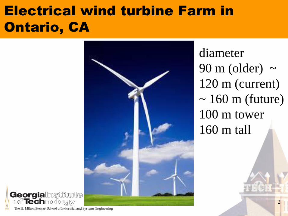
Electrical wind turbine Farm in
Ontario, CA
2
diameter
90 m (older) ~
120 m (current)
~ 160 m (future)
100 m tower
160 m tall

Wind Turbine Components
Components of a Wind Turbine (Liu and Chu 2012)
4/20

Wind Turbine Blades Transportation
by Rail
4/20
(Source: www.vestas.com)

(Source: www.nrel.gov)
Wind Turbine Components using
Truck Transportation
5

Problem Characteristics
Problem is highly supply constrained
Specialized suppliers with long lead times
Ordering from suppliers is done before uncertainty is
revealed
After it is revealed, products flow, demand fulfilled
If supply < demand: backorders and lost sales
If supply > demand: inventory and capacity expansions
In wind turbines supply chains:
Renting off-site storing for parts that arrived early
Arrangement for transportation
6/20

Supplier Uncertainty
Suppliers’ uncertainty
Demand uncertainty is most commonly studied
Components of Uncertainty in supply/supplier are:
Uncertainty in costs and capacities (e.g. Alonso-Ayuso
et al. 2003 & 2007, Santoso et al. 2005)
Random yield (e.g. Bollapragada and Morton 1999)
And/or random lead times (e.g. Dolgui et al. 2002)
Uncertainty studied: random yield + stochastic
lead times
8/20

Modeling General Supplier
Uncertainty
10/20

Model Development Highlights
11/20
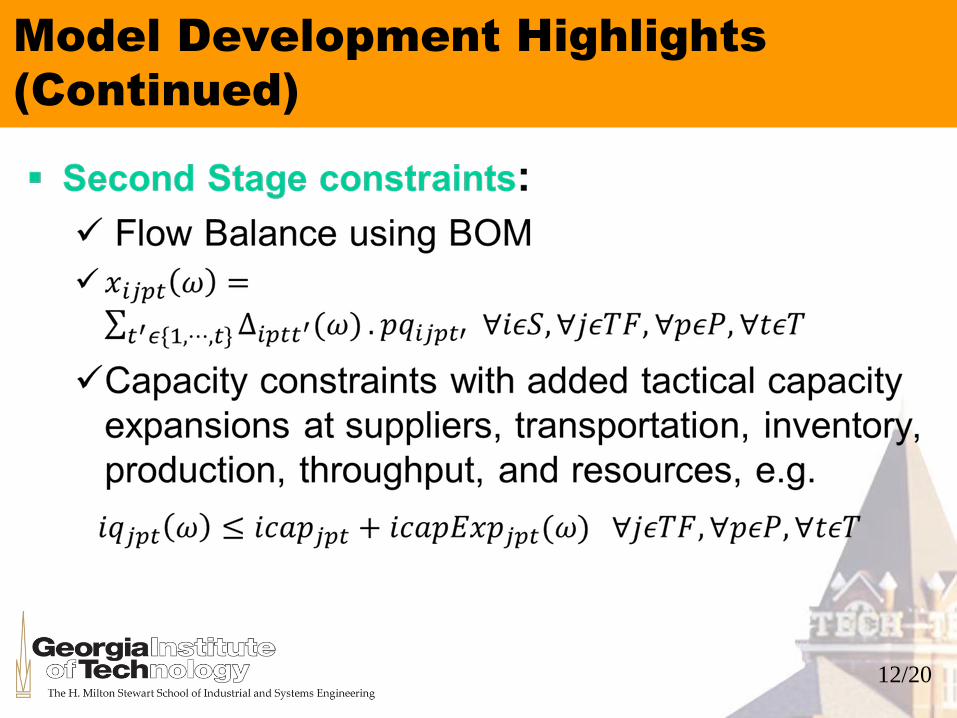
Model Development Highlights
(Continued)
12/20
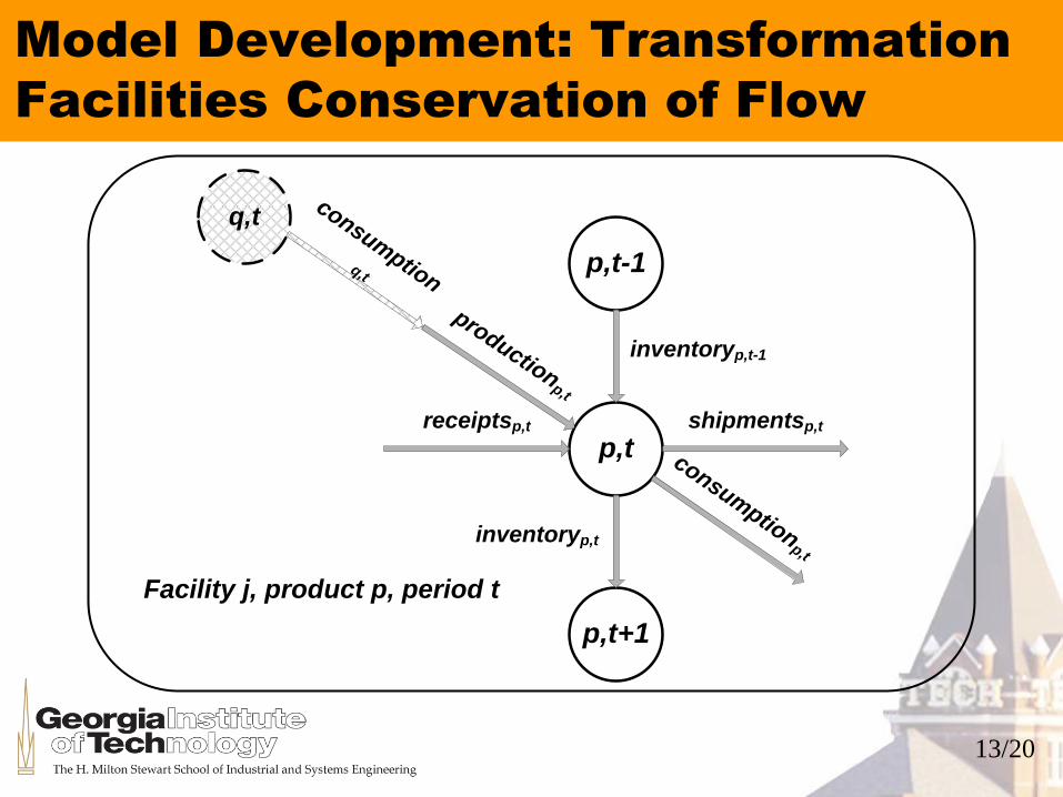
Model Development: Transformation
Facilities Conservation of Flow
p,treceiptsp,t shipmentsp,t
p,t-1
inventoryp,t-1
p,t+1
inventoryp,t
productionp,t
consumption
p,t
q,tconsum
ptionq,t
Facility j, product p, period t
13/20
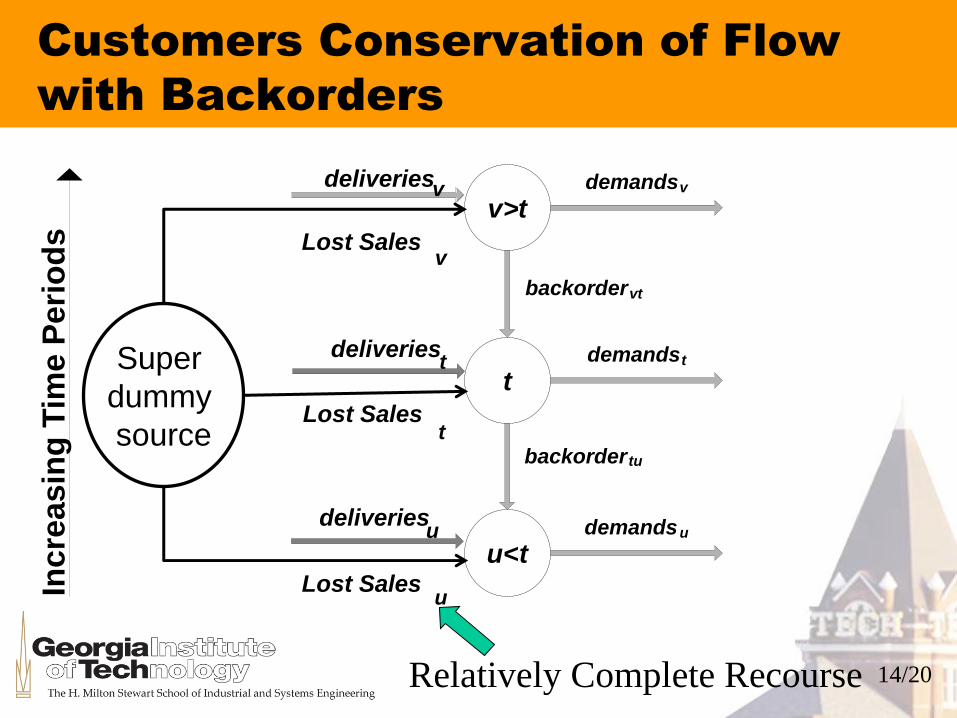
Customers Conservation of Flow
with Backorders
t t demands t
v > t
backorder vt
u < t
deliveries v demands v
backorder tu
demands u
Inc
reasin
g T
ime P
eri
od
s
Lost Sales v
deliveries
Lost Sales
deliveries
Lost Sales
t
u
u
Relatively Complete Recourse
Super
dummy
source
14/20

Optimal Solution May Order More
than the Deterministic Demand
…. 1 2 3
Solution = Order 10 units
Demand = 10 units at period 1
Deterministic Problem
Optimal Solution
…. 1 2 3
Order 10,
receive 5
Expected Value or One-Scenario Problem
2 is optimal if purchasing
+ inventory < backorder
…. 1 2 3
Order 20,
receive 10 receive 10
receive 5
Inventory Backorder
15/20
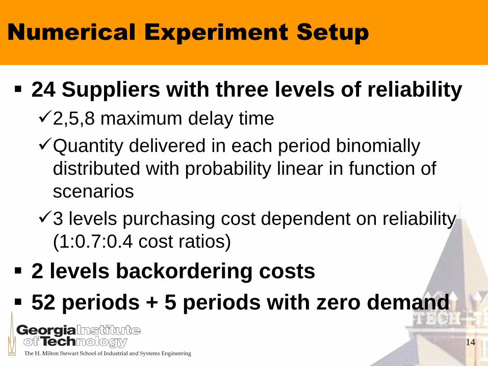
24 Suppliers with three levels of reliability
2,5,8 maximum delay time
Quantity delivered in each period binomially
distributed with probability linear in function of
scenarios
3 levels purchasing cost dependent on reliability
(1:0.7:0.4 cost ratios)
2 levels backordering costs
52 periods + 5 periods with zero demand
Numerical Experiment Setup
14

50 Scenarios
Numerical Experiment Setup
(Continued)
15

Database: Microsoft Access
Model: GPML
MIP Solver: CPLEX 12.2
Computer: T7200, 6 MB RAM
Deterministic Equivalent Problem (DEP)
with default parameters (no
decomposition)
LP Model generation 25 minutes
Model solution < 0.2 minutes
Numerical Experiment Execution
16

Results of Numerical Experiment:
Sourcing from Unreliable Suppliers
17
Backorder
Cost LevelPurchasing Cost Level
Cost
Increase
over
100%
Reliable
%
Procure
ment
Most
Reliable
%
Procure
ment
Medium
Reliable
%
Procure
ment
Least
Reliable
%
Procure
ment
over
Demand
Low Low and Equal for All Suppliers 1.51 62.34 11.08 26.58 0
High Low and Equal for All Suppliers 3.12 69.71 13.13 17.16 0.09
Low High and Equal for All Suppliers 0.09 44.67 18.48 36.85 0
High High and Equal for All Suppliers 0.27 50.99 20.03 28.98 0
Low High with More Reliable Suppliers Being More Expensive 0.62 0 0 100 0
High High with More Reliable Suppliers Being More Expensive 4.15 0 1.94 98.06 0.45
Low Low with More Reliable Suppliers Being More Expensive 9.72 0 2.01 97.99 0
High Low with More Reliable Suppliers Being More Expensive 20.79 2.1 1.83 96.06 3.71

Results of Numerical Experiment
18
Backorder
Cost LevelPurchasing Cost Level
%
Procure
ment
Most
Reliable
%
Procure
ment
Medium
Reliable
%
Procure
ment
Least
Reliable
%
Procure
ment
over
Demand
% Cost
EVP
below
MVP
Low Low and Equal for All Suppliers 51.38 9.99 38.63 0 1.44
High Low and Equal for All Suppliers 52.87 10.54 36.59 0.26 2.57
Low High and Equal for All Suppliers 41.83 16.85 41.32 0 0.09
High High and Equal for All Suppliers 41.38 17.17 41.44 0 0.19
Low High with More Reliable Suppliers Being More Expensive 0 0 100 0 0.6
High High with More Reliable Suppliers Being More Expensive 0 0 100 0.04 3.92
Low Low with More Reliable Suppliers Being More Expensive 0 0 100 0 9.5
High Low with More Reliable Suppliers Being More Expensive 0 0.03 99.97 0.69 19.55
EVP: expected value problem (stochastic)
MVP: mean value problem (deterministic)

Cheapest suppliers are selected
regardless of reliability
Expected Value Problem cost more than
deterministic problem (100% reliable)
Excess purchasing only for large
backorder cost and small purchasing cost
Cost increase EVP over deterministic
(100% reliable) grows with backorder cost
Results of Numerical Experiment
19

% cost decrease of EVP versus MVP (VSS)
increases with backorder costs
Decisions of the model cannot be
predicted by “intuition” or rules of thumb,
a mathematical modes is required
Procurement source and quantity and timing
(purchase + transport cost), inventory, backorder,
and excess procurement are extremely
interdependent
Results of Numerical Experiment
(Continued)
20

Conclusions
A 2-stage stochastic programming model for
comprehensive tactical supply chain planning
under supplier uncertainty was developed
Uncertainty/unreliability of suppliers in one of
its most general forms is modeled
A direct real-world application is in the wind
turbines industry
Optimal procurement quantities when
considering supplier uncertainty might be
larger than deterministic demand
18/20

Conclusions (Continued)
Model chooses cheapest suppliers, regardless
of their reliability
Solution of Expected/mean value problem >
deterministic problem
% relative difference in costs increases when
backorder costs get higher
VSS/stochastic solution reached values of up to
20%
19/20

May I answer any questions?
24