1

Product Demand Characteristics, Brand Perception, and

Financial Policy

Yelena Larkin*

Cornell University

November 15, 2010

Job Market Paper

Abstract

We use a proprietary database of consumer brand evaluation to explore the role of firm-specific

demand characteristics in financial decisions. We hypothesize that higher and more inelastic

consumer demand for a product reduces the costs of financial distress but can also intensify

agency conflicts by increasing firm market power. The empirical analysis shows that firms with

stronger demand take on more debt and hold less cash, suggesting that financial distress risk is

the primary channel through which brand value affects financial policy. To address endogeneity

issues, we instrument for characteristics of product demand by using extreme consumer

responses about the actual usage of the brands and arrive at similar conclusions. Taken together,

the results suggest that features of demand for a firm’s products affect financial decisions and

allow the firm to have higher leverage and smaller cash cushions.

*Correspondence should be addressed to Johnson School of Management, 301 Sage Hall, Cornell University, Ithaca,

NY 14853. E-mail: YL429@cornell.edu. I am thankful to Roni Michaely, Yaniv Grinstein, Mark Leary, and Vithala

Rao for very helpful comments and suggestions. I am also grateful to Alyssa Anderson and seminar participants at

Cornell University and Syracuse University. The remaining errors are my own. I am deeply grateful to Brand Asset

Consulting, and especially to Ed Lebar, for providing me with access to the data and guidance on its use.

1

Extensive theoretical and empirical literature has examined the interaction between

financial and real policy of a firm. A large group of studies has focused on the relationship

between financial policy and industry factors, such as concentration ratio and competition

(Chevalier (1995a, 1995b), Kovenock and Phillips (1995, 1997), Phillips (1995), Khanna and

Tice (2000)), firm’s relative technological position (MacKay and Phillips (2005)), and

interdependence between operation of a firm and its rivals (Lyandres (2006)). At a firm level,

studies have examined the interaction between capital structure and characteristics of the supply

side, such as the flexibility of the production function (MacKay (2003)) and investments in R&D

(Opler and Titman (1994)). Still, little is known about the interaction of the demand side with a

firm’s financial policy.

This study complements previous research by analyzing the cross-sectional variation in

demand characteristics of the product market at a firm level. It explores the role of firm-specific

demand characteristics in financial decisions using a proprietary database that measures unique

attributes of product demand across firms. The database, Brand Asset Valuator (BAV), is the

world’s largest study of consumer evaluation across different product brands and has never been

used in financial research.1 Overall, the concept of brand can be defined as a ―name, term,

symbol or design … intended to identify the goods and services of one seller or group of sellers

and to differentiate them from those of competitors.‖2 Research in marketing has demonstrated

that favorable consumer evaluations of a brand are associated with higher loyalty, higher

perception of quality, and larger purchase probabilities (Starr and Rubinson (1978), Rao and

Monroe (1989), Dodds, Monroe, and Grewal (1991)). As a result, consumer opinions about how

much they value a brand are a natural candidate to capture demand characteristics of a firm. We

aggregate consumer responses on measures of how well they know and value a brand to

construct our main proxy of product demand characteristics (brand Stature).

Why are demand characteristics important? A critical assumption of perfect competition

is that sellers provide homogeneous, or standard, goods. However, in practice, the majority of

firms produce goods with somewhat different properties (or at least goods that are perceived

differently by consumers). Product differentiation creates ―monopolistic competition,‖ in which a

firm’s market becomes separated to a degree from its competitors (Chamberlin (1933)), and as a

1 Published academic studies, based on BAV data, include Mizik and Jacobson (2008, 2009), Bronnenberg, Dhar,

and Dube (2007, 2009) and Romaniuk, Sharp, and Ehrenberg (2007). 2 According to the American Marketing Association (AMA).

2

result, every firm faces a different demand curve. A shifted out and inelastic demand curve

allows a firm to better utilize its monopolistic power and set higher prices, indicating a larger and

more stable consumer base and higher market power of a firm compared to competitors.

How should those demand characteristics affect financial decisions? One effect is that

higher and more inelastic demand reduces the expected costs of financial distress, as firms are

less likely to face low states of cash flow realization. Firms with strong demand are also less

prone to predatory behavior by competitors. As a result, strong consumer demand enhances the

debt capacity of a firm. In addition, a firm with high and inelastic demand enjoys larger and

more certain future cash flow and, therefore, can hold less cash for precautionary reasons and

distribute more to its shareholders.

At the same time, inelastic demand reduces a firm’s sensitivity to peer competition.

Market competition is considered to be one of the managerial disciplining devices (Allen and

Gale (2000)). Grullon and Michaely (2007) support this argument by demonstrating that firms in

less competitive industries pay out less. Agency conflicts generates opposite predictions about

the relations between demand function characteristics and a firm’s financial decisions. Since

stable consumer demand improves a firm’s relative positioning among other firms and reduces

the impact of market competition on a firm, agency problems between managers and

shareholders intensify. As an outcome, firms with string demand hoard cash and distribute less to

the shareholders. Firms might also choose to hold less debt, as debt also restricts managerial

discretion (Jensen (1986)).

We empirically examine the two hypotheses about the effect of demand function

characteristics on financial policy. The first hypothesis states that the market friction that links

demand characteristics to a firm’s decisions is costs of financial distress. Firms with higher and

more inelastic demand have lower costs of financial distress, which allows them to hold more

debt and less cash and to pay out more. The second hypothesis is an outcome of intensified

agency problems, and predicts that a strong demand for a firm’s products reduces the

disciplinary role of market competition and, consequently, firms hold less debt, hoard cash, and

pay out less. Whether demand characteristics are related to a firm’s financial channel and which

of the mechanisms determines the relationship is an open empirical question.

We estimate each of the dependent variables (leverage, cash holdings, and payout ratio of

a firm) as a function of brand Stature, the aggregate measure of demand characteristics, and a set

of commonly used control variables and demonstrate that the properties of consumer demand

3

have an economically and statistically significant impact on capital structure and cash holdings.

The empirical results provide support for the first hypothesis, suggesting that the impact of

consumer demand on the costs of financial distress dominates its impact through more acute

agency problems. We find that firms with stronger demand hold more leverage: a one-standard

deviation increase in brand Stature increases debt holdings by about 16%. Those firms also hold

less cash, compared to firms with similar accounting and financial characteristics. We do not find

a robust impact of consumer demand on payout policy. While the general relation is, overall,

positive, it is not statistically significant in all specifications. To understand more deeply the

relative contribution of consumer demand characteristics, we perform a variance decomposition

analysis and find that Stature contributes to the explanatory power at least as much as the

standard control variables, suggesting that it can be responsible for the large component of the

firm fixed effects in cross-sectional leverage estimation. Taken together, the results suggest that

consumer demand characteristics are important in explaining financial policy of a firm, and

financial distress risk is the primary channel through which consumer demand affects financial

policy.

We perform additional tests to enhance the validity of our main results. For example, the

results above can be explained also by the substitution model of agency costs. If managers of

firms with strong demand anticipate a harshening of agency problems, they may voluntarily

restrict themselves from potential overuse of a firm’s funds. By choosing higher debt levels,

lower cash reserves, and higher payouts, they are able to maintain a favorable reputation of

operating in the best interests of the shareholders. To address this concern, we use the

entrenchment index of the corporate governance provisions, suggested by Bebchuk, Cohen, and

Ferrell (2009). If managers are indeed willing to forego some of the power to signal their

intentions, we should observe a lower corporate governance index for firms with stronger

demand. However, we find that entrenchment index is actually higher among those firms,

consistent with the outcome, rather than substitution, explanation. Including the entrenchment

index to the regression specifications does not influence the main results.

Another obvious concern for the validity of the results above is the issue of endogeneity.

Firms may try to affect consumer demand by improving the quality of their products or altering

consumer opinions about the brand through advertising. The reverse causality argument predicts

that a firm’s capital structure determines how aggressively it competes in prices, R&D, and

4

advertising.3 Some omitted factors may also play a role. To address those issues, we use a piece

of the BAV survey data that is correlated with consumer view of a brand but is unlikely to be

correlated with the firms’ financial policy. Specifically, we use the percentage of household

responses to the questions ―the one I prefer to buy/use‖ and ―the one I would never buy/use‖ as

instruments for consumer perception of a product. The variables have several advantages. First,

they are formed through an individual experience of respondents with a certain brand and,

therefore, better reflect the match (mismatch) between product qualities and consumer

preferences. Second, due to their intensity, these measures are not likely to be affected by the

contemporaneous market policy of a firm, such as price cuts or extensive advertising.4 We re-

estimate the main regressions using 2SLS technique and find support for the main results that

stronger consumer demand has a positive impact on capital structure and a negative impact on

cash holdings.

This paper makes several contributions to the existing research. First, it adds to the

literature on product market and financial decisions by identifying potential channels that link

characteristics of consumer product demand to financial decisions of a firm and evaluates the

impact of those characteristics. While previous studies on product market characteristics mainly

focus on capital structure decisions, this paper takes a broader approach and explores a variety of

a firm’s financial policy components (capital structure, cash holding, and payout).

Second, this paper complements capital structure research that examines the link between

the properties of a firm’s assets/liabilities and financial leverage. Although recent studies have

mainly focused on the impact of tangible assets characteristics (Benmelech (2009), Benmelech

and Bergman (2009), Campello and Giambona (2010)), little has been done to examine

characteristics of the intangible side of the assets. While the literature so far concludes that

capital can be borrowed mainly against tangible assets (Rampini and Vaswinathan (2010)), this

paper demonstrates that characteristics of the firm’s intangible assets, such as brand stature, also

provide debt capacity. As a result, this study adds to the relatively limited literature on how the

properties of the off-balance sheet assets and liabilities, such as leases and pension plans

(Graham, Lemmon, and Schallheim (1998), Shivdasani and Stefanescu (2009)), affect the firm’s

financial activities. In addition, this paper introduces an alternative forward-looking measure of

3 See, for example, theoretical models by Brander and Lewis (1986) and Bolton and Scharfstein (1990).

4 Literature in psychology has provided extensive evidence that strong attitudes are resistant to change, persistent

over time, and predictive of behavior (Pomerantz et al. (1995)).

5

cash flow volatility and addresses the mixed empirical conclusions on the relations between cash

flow volatility and capital structure.5

Lastly, this study contributes to a small number of finance papers that map marketing

concepts, such as advertising and brand perception, into financial theory. Most of those studies

look at the link between firm characteristics and advertising (Grullon, Kanatas, and Weston

(2004)), Chemmanur and Yan (2010a, 2010b). Additional studies examine the relations between

advertising and capital structure decisions (Chemmanur and Yan (2009), Grullon, Kanatas, and

Kumar (2006)). Finally, Frieder and Subrahmanyam (2005) examine the impact of brand on a

firm’s ownership structure. Our study incorporates a new data set that captures consumer

subjective evaluation of a firm’s products and demonstrates that, in addition to visibility created

by advertising, marketing characteristics interact with firm’s financial decisions through other

channels. More broadly, the study emphasizes the link between the fields of marketing and

finance and suggests that marketing policy, such as brand management, and financial policy,

such as capital and cash holding decisions, are interdependent.

The rest of the paper is organized as follows: Section I develops the main hypotheses of

the paper; Section II describes the data; and Section III presents the main results. In Section IV

we address the endogeneity concerns, and Section V verifies the robustness of our conclusion,

replicating the main results across different subsamples and variable definitions. Section VI

concludes.

I. Theory and Empirical Hypotheses

In this section we develop the hypotheses of the paper. We start by explaining how

consumer opinions about firm products translate into characteristics of a firm’s demand. We then

separately discuss two potential channels through which the demand function can affect

managerial decisions to hold debt, retain cash, and pay out to shareholders and generate a set of

testable predictions for each channel.

Marketing and economic research has long attempted to identify and estimate the demand

curve of a product. The best possible way to measure demand is through scanner data, through

which researchers observe actual sales at the level of an individual purchase. The problem is that

while providing precise estimates of price-quantity relations, the data usually do not have

5 Parsons and Titman (2008) provide an overview of existing literature on the topic (pp. 14–16).

6

sufficient product cross-section and typically focus on only 2 to 3 types of brands. These studies

are also conducted over a short period of time and are often limited to certain geographic

locations. Consumer surveys are the second best solution. While the degree of precision is

somewhat lower (for example, a consumer can report a favorable opinion about a brand, but still

purchase a different one), these surveys allow a substantial expansion of the sample across

different products, geographical regions, and time periods.

Marketing studies have used consumer surveys to show that favorable consumer

evaluations of a brand are associated with their perception of quality, loyalty, price they are

willing to pay, and the probability of switching to competitors. Using survey questions, Starr and

Rubinson (1978) allocate consumers into loyalty groups and find that loyal consumers have

higher repeat rates of purchase, lower probability of switching, and lower price elasticity of the

demand function.6 Based on an experimental approach, Dodds et al. (1991) show that when

brand perception is more favorable, consumers attribute higher quality to the product, and their

perception of the product’s value and the overall willingness to purchase is greater. Rao and

Monroe (1989) perform a meta-analysis of previous studies and conclude that brand name has an

impact on a consumer’s evaluation of product quality. Finally, Aaker (1996, p. 17) summarizes a

set of studies, based on detailed data of business units (PIMS) that show that perceived quality

contributes to a firm’s profitability by enhancing prices and market share.

The marketing studies above demonstrate that consumer surveys provide valuable

information about characteristics of a product demand even if they do not precisely capture the

demand curve. First of all, consumer brand perception indicates how shifted out the demand

curve is: the higher the subjective value of the unit of good for a consumer is, the more he or she

is willing to pay for a unit of it. Some marketing studies actually use the difference in prices of a

specific product among different brands to derive a quantitative measure of consumer loyalty

(Aaker (1996), p. 320). Another important characteristic of demand is its sensitivity to price

changes by the firm and competitors, as well as other factors, such as combat advertising.

Elasticity is important in a context of monopolistic competition, when a firm observes down-

sloping, rather than infinitely elastic demand, consistent with perfect competition. The individual

characteristics of each brand separate the overall demand for a product into individual firm’s

6 Since the demand curve is typically downward sloping, elasticity and slope of the demand curve take on negative

values. For the sake of clarity we will always refer to the absolute values of elasticity and slope when discussing the

characteristics of the demand curve.

7

demands, and impose firms with a maximization problem of a monopoly (Chamberlin (1933)).

Consumer loyalty, characterized by inelastic demand, allows a firm to set higher prices. In

addition, it reduces the probability that a consumer will switch to a different brand, insulating the

firm from predatory behavior and entries of new firms into the industry.

In the remainder of the section, we incorporate the characteristics of consumer demand

into the theory of financial decisions and establish its impact on leverage, cash holdings, and

payout policy.

1. Costs of financial distress

Costs of financial distress are one of the most fundamental frictions of financial markets.

While the original framework of Modigliani and Miller (1958) does allow for liquidation of a

firm in the case of low cash flow realization, it is the indirect costs associated with the distress

states that create the distortion. As a result, firms care both about the overall costs of financial

distress and about the probability of getting into it. Strong consumer demand, in terms of a

higher and more inelastic demand curve, reduces costs of financial distress for several reasons.

First, firms are less likely to face low states of cash flow realization, for example, during market

downturns. Loyal consumers will rebalance their consumption baskets in a way that minimizes

the cut of products that they value the most. In addition, firms with strong demand are less prone

to predatory behavior by competitors, who can strategically drive them into bankruptcy.

While the link between characteristics of consumer demand and a firm’s stability has not

been directly addressed in financial studies, substantial marketing literature has explored the

impact of consumer satisfaction and brand perception on the overall riskiness of a firm. Several

studies have examined the impact of the American Customer Satisfaction Index on systematic

and idiosyncratic risk of the firm (Fornell, Mithas, Morgenson, and Krishnan (2006), Madden,

Fehle, and Fournier (2006), Tuli and Bharadwaj (2009)) and the volatility of the cash flow

(Gruca and Rego (2005)) and found that higher consumer satisfaction reduces both types of

risks. McAlister, Srinivasan, and Kim (2006) show that advertising and R&D expenses also

reduce systematic risk of a firm. Finally, studies by Anderson and Mansi (2009) and Rego,

Billett, and Morgan (2009) find that higher customer satisfaction and brand value improve credit

ratings and Z-scores and lead to a lower cost of debt capital. Overall, marketing literature

provides robust evidence that brand perception indeed reduces the riskiness of a firm.

8

Taken together, the evidence above suggests that firms that have stronger demand in

terms of having a loyal pool of satisfied consumers who value the brand more experience more

stable cash flow. As a result, the expected costs of financial distress are lower and the debt

capacity of a firm can be higher.

Hypothesis 1a: Firms with stronger consumer demand have higher leverage.

The impact of consumer demand on a firm’s cash holding decision mirrors the decision

of capital structure: Firms will choose to insure themselves against losses associated with distress

state realization by holding more liquid assets (Opler, Pinkowitz, Stulz, and Williamson (1999),

Bates, Kahle, and Stulz (2009)). Since raising external capital is typically costly (either because

of the direct fees to the intermediary or as an outcome of asymmetric information problems

between the firm and outside investors), firms hold a certain proportion of their retained earnings

in cash and other liquid assets as a cushion. When a firm has a secure stream of future cash

flows, as proxied by the characteristics of the product demand, the need to hold cash for

precautionary reasons lessens: Operating cash flow provides a ready source of liquidity and

allows firms to maintain lower levels of cash at any given point (Kim, Mauer, and Sherman

(1998)). In addition, firms usually hoard cash as a means to fight peer predation. A loyal

consumer base implies that predatory behavior is costly for competitors, and as a result, a firm

with strong demand can hold less cash.

Hypothesis 1b: Firms with stronger consumer demand have lower cash holdings.

If firms with strong demand are more profitable and do not need to hold much cash, they

can distribute more to their shareholders in terms of dividends or repurchases. This leads to the

last hypothesis of this subsection:

Hypothesis 1c: Firms with stronger consumer demand pay out more.

2. Agency costs

Another potentially important market friction is agency costs of managerial discretion, in

cases in which managers do not operate in the best interests of the shareholders. While

substantial literature in corporate finance has addressed the overall determinants of agency

9

problems, Allen and Gale (2000) summarize a theoretical framework that shows that competition

among firms may serve as an effective corporate governance mechanism. Managers of firms,

operating in a competitive industry, cannot engage in suboptimal behavior, maximizing their

utility at the expense of shareholders, as it impairs the power of a firm to compete in the product

market and can eventually drive the firm into financial distress. Grullon and Michaely (2007)

find empirical support for the validity of this argument by showing that disciplinary forces of

market competition force managers of firms, operating in less concentrated industries, to pay out

more.

A strong demand for a firm’s products insulates it from the competitive environment of

the rest of the industry and reduces the firm’s sensitivity to peer strategic behavior. As a result,

for any given level of industry competition, a firm with stronger demand is subject to less

competitive force. Reduced competition may have an impact on managerial behavior and

intensify agency problems. As a result, the channel of agency costs generates a different set of

predictions about the link between consumer demand and financial policy.

The implications for debt are as follows. Previous research has shown that debt

disciplines managers by improving the shareholder information about a firm’s operations and

managerial skills, and imposing a liquidation threat (Harris and Raviv (1990)). As a result, if

managers have control over the debt level, they will prefer less leverage. Higher debt also

increases the probability of a firm going into distress, and this is an outcome that a risk-averse

manager would like to avoid. As an outcome, if strong demand for a firm’s products intensifies

the agency problems, managers will try to reduce their debt holding.

Hypothesis 2a: Firms with stronger consumer demand have lower leverage.

Finally, managers who are not properly monitored will try to hoard more cash and pay

out less to shareholders. Since managers are risk-averse, they put more emphasis on

precautionary motives of holding liquid assets. They also prefer to keep more cash within the

firm for their personal benefits (Opler et al. (1999)). As managers try to retain a higher

proportion of the earnings, they become reluctant to pay out dividends to the shareholders, or

repurchase stock. Therefore, if stronger demand intensifies conflicts between managers and

shareholders, managers will have higher cash reserves and smaller payouts.

10

Hypothesis 2b: Firms with stronger consumer demand have higher cash holdings.

Hypothesis 2c: Firms with stronger consumer demand have lower payouts.

II. Data

1. Brand perception versus advertising

An extensive work in industrial organization has examined how advertising affects demand,

share stability, and consumer loyalty. However, while advertising can be a good proxy for a

firm’s overall visibility, it is just one of many inputs that a firm uses to affect consumer view of a

product. At the same time, brand perception measures the outcome of all the cumulative efforts

of a firm to market the product, as well as all other exogenous factors, such as the fit between

consumer preferences and product characteristics.

Moreover, advertising is clearly an endogenous variable of a firm. For example, while there

may be a link between profitability and advertising, it is not clear whether advertising leads to

higher profit margins, or profitable firms can spend more on advertising. Consumer brand

perception, on the other side, conveys the goodness of fit between style and general

characteristics of a brand and individual preferences of consumers, and as a result, carries a

larger exogenous component.

Overall, using consumer views of a brand provides a cleaner measure of their actual

preferences. The higher the consumer’s opinion of the brand, the higher the price he or she is

willing to pay and/or the larger the amount purchased. As a result, consumers’ regard for a brand

directly translates into how far out is its demand curve shifted. Similar logic applies to brand

loyalty. The higher a consumer’s satisfaction with the product, the less likely he or she is to

switch to the products of competitors. As a result, consumer responses provide additional

information about the elasticity of the demand curve. Unfortunately, the data that records cross-

industry variation in consumer responses are very limited. BAV is one of a few databases that

provide panel-type data on consumer brand perception, and its contribution to reconciling

different theories of advertising is yet to be established. The next subsection describes the nature

of the BAV data in more detail.

2. Brand Asset Valuator

Brand Asset Valuator (BAV) is a proprietary brand metrics model, developed and managed

by Brand Asset Consulting, a subsidiary of Young & Rubicam Brands. Brand Asset Consulting

11

uses the model to help clients evaluate their brand and improve the strategic direction of its

management by analyzing different aspects of brand image. The model is widely known among

both marketing researchers and practitioners and is incorporated in major marketing textbooks

(see, for example, Aaker (1996) and Keller (2008)).

The BAV model has several advantages over other marketing models that measure brand

value. Most importantly, it relies on a customer-based approach. This is in contrast to a financial

valuation approach, which relies on accounting and financial data to estimate the brand value.

For example, models by Interbrand and BrandFinance 2000 are based on cash flow forecasts. As

a result, the BAV model is exogenous of accounting and market variables, such as stock prices,

B/M ratios, and revenues. Second, the model has a wide base of respondents: It is a survey of

nearly 16,000 US households7 who evaluate each brand with respect to a wide range of

characteristics. The sample of US households is constructed and managed to represent the US

population, according to the following factors: gender, ethnicity, age and income groups, and

geographic location. Households are offered a $5 compensation for their participation, and the

response rates are more than 65%. The pilot surveys have been conducted in 1993, 1997 and

1999, and starting from 2001, the survey has been undertaken yearly.

The list of brands has expanded over time and as of 2009 included more than 4,000 US and

international brands and subbrands.8 The survey is not limited to companies that are customers of

Brand Asset Consulting and is continuously updated to include new brands and remove the

brands that exit the market. Overall, the sample of firms is representative of all industries and is

not biased towards the clients of Brand Asset Consulting. In order to make the questionnaires

manageable, the overall sample of brands is split into 30 groups, so that the average number of

brands to be evaluated per questionnaire does not exceed 120.9 BAV metrics uses a

randomization approach in organizing the brands in the questionnaires in order to not impose

associations with a certain industry or firm competitors.

BAV questionnaire consists of two types of questions. The first type asks respondents to

evaluate the following aspects of a brand on a 7-point scale: general knowledge of the brand,

personal regard and relevance. The second type evaluates different aspects of brand image and

7 In addition to US studies, BAV also conducts international studies of consumers.

8 Additional models, based on customer based approach, are Landor Associates, which covers around 300 brands,

and EquiTrend, which covers more than 1,000. Landor Associates’ ImagePower, which was the first model of

consumer-based surveys, was expanded into BAV in the early 1990s. 9 See Appendix 1 for an example of a questionnaire page.

12

asks participants to mark an ―X‖ if a certain characteristic applies. The examples of the

characteristics are: unique, innovative, traditional, good value. Additional questions ask

respondents about the frequency of use of a certain brand, and also some demographic

information.

The overall results are aggregated across respondents for any given brand-year, so that we

observe the overall score on a certain brand’s image characteristics but cannot identify individual

respondents. Some of the brand-image results are aggregated into pillars that capture different

aspects of brand value, and some are used for additional marketing analysis of brand

characteristics. Brand Knowledge and Esteem constitute brand Stature, which we use as our main

measure of brand loyalty and quality perception. The components of Esteem are (1) the

proportions of respondents who consider the brand to be of ―high quality,‖ a ―leader,‖ and

―reliable‖; (2) brand score on Regard (―how highly you think and feel about the brand‖ on a 7-

point scale). Bronnenberg, Dhar, and Dube (2007, 2009) use the percentage of responses to the

―high quality‖ question, as well as the response rates to two additional questions, ―good value‖

and ―best brand,‖ as their main measure of demand-related brand performance. We follow their

approach, but use all the components of Esteem, as well as consumer’s Knowledge of the brand

(―how well are you familiar with the brand and its products?‖ on a 7-point scale). The reason for

using a more general measure is twofold. First, the BAV model describes brand Stature, the

combination of Esteem and Knowledge, as an indicator of the current perception of a brand by

consumers (Gerzema and Lebar (2008), pp. 44–45), and we do not have a theoretical reason to

exclude any of its components. Second, the knowledge of a brand is an essential part of building

a demand curve, as consumers who are not familiar with the brand should not be included in the

demand function. While we believe that brand Stature is a more general measure of consumer

demand than the one that includes only selective components of Esteem, we address additional

definitions in the robustness section.

Stature is computed as a product of Esteem and Knowledge. Since the two components are

estimated on different scales its absolute value is meaningless. For convenient interpretation of

the results, we transform the measure into a z-score.

The BAV questionnaire is constructed at a brand level, so in order to merge it with the

commonly used financial data, which is reported at a firm level, we have manually created a

bridge that links between BAV and Compustat. Appendix 2 provides a detailed description of the

algorithm we apply to construct the link.

13

3. Financial variables

The financial variables are selected based on the commonly cited literature on capital

structure, payout policy, and cash holdings.10

We merge several different databases to construct

them. First, we use Compustat data to obtain accounting and financial variables. Size is the

overall book assets, expressed in millions of constant 1993 dollars. Age of the firm is calculated

starting from the first year the firm appeared in the Compustat database. Market to book ratio

(M/B) is the market value of equity plus the book value of assets minus preferred stock11

plus

deferred taxes, all divided by the book value of assets. EBITDA is the ratio of operating income

before depreciation to total assets. Leverage is the sum of short-term and long-term debt, scaled

by book assets. We measure the tangibility of a firm’s assets with two measures. First, we use

Tangibility, defined as net property, plant, and equipment, divided by book assets. We also use

Depreciation, scaled by assets, as an additional measure of tangible assets.

We measure advertising and R&D expenses in two ways. For the sample description, we

scale advertising expenses and R&D by assets. For multivariate analysis, we use the natural

logarithm of the overall amount of advertising and R&D (in millions of constant 1993 dollars)

(variables log(advertising) and log(R&D), respectively).12

Following Grullon et al. (2004), we do

not scale advertising by assets or sales to capture its overall scope.13

If advertising affects

consumer demand, it should be captured by the overall amount of advertising consumers were

exposed to. An advertising campaign of a large firm can be effective even if it represents only a

small proportion of a firm’s revenues. For the same reason, we use log(R&D) rather than its ratio

over assets or sales to capture a potential impact of a firm on the demand curve through

improving the quality of its products. Using the overall amount of advertising and R&D in our

empirical estimations will better differentiate the effect of exogenous brand characteristics from

10

See, among others, Hovakimian, Opler, Titman (2001), Fama and French (2002), Faulkender and Petersen (2006),

Opler, Pinkowitz, Stulz, and Williamson (1999), Kim, Mauer, and Sherman (1998), Grullon and Michaely (2002),

Grinstein and Michaely (2005). 11

The book value of equity is the book value of total assets minus book liabilities minus preferred stock plus

deferred taxes. Preferred stock equals to the liquidation value if not missing; otherwise I use redemption value if not

missing; otherwise the carrying value. 12

We add a value of 1 to advertising and R&D expenses, before converting them to logarithms, to capture the

values of zero. 13

Differently from Grullon et al. (2004), we assign values of zero for missing values of advertising expenditures.

Since firms do not have to report advertising expenses (following the SEC’s Financial Reporting Release No. 44

FRR44)), this is not entirely accurate. However, it preserves the number of observations. For robustness, we repeat

the main analysis using only nonmissing values of advertising expenses, and the results are almost the same.

14

the firm’s attempts to alter consumer demand through advertising and R&D and make our tests

more conservative.

We measure cash holdings in two ways. Our main measure is Cash, the ratio of cash and

short-term investments to total assets. For robustness, we also scale cash by sales (CashSales).

Following Opler et al. (1999), we use working capital net of cash holdings (Wcap), scaled by

assets, to capture additional liquid asset substitutes available to a firm. Since a firm with more

projects to finance should hold more cash, we use a measure of capital expenditures (CapEx) to

proxy for required investments. We capture how easily a firm can access external markets by

using Access, which is a dummy variable that equals to one if a firm has a credit rating for any of

the debt it holds and zero otherwise. S&P500 is a dummy variable that equals one if a firm

belongs to the S&P 500 index and zero otherwise. This dummy variable is another proxy for size

and also a reflection of additional stock characteristics, such as visibility, liquidity, and

institutional holding.

We construct several measures of payout. We define dividends as total dollar amount of

dividends declared on the common stock of the firm during the year. DivDummy is a dummy

variable that equals one if a firm pays out dividends, and zero otherwise. Similarly, RepoDummy

takes a value of one if a firm repurchases and zero otherwise; and TotDummy takes a value of 1

if either dividends or repurchases are positive and zero otherwise. Following Grullon and

Michaely (2002), we define repurchases as total expenditure on the purchase of common and

preferred stocks minus the reduction in the value (redemption value) of the net number of

preferred stocks outstanding.

A potential concern of any study that relies on brand data is that conceptually, the idea of

a brand is industry specific. To avoid capturing industry, rather than firm product characteristics,

we control for industry characteristics in several ways. First, we include the Herfindahl industry

concentration ratio in all our regressions. We create a Herfindahl index (HHI) by summing up

squared market shares of all the publicly traded companies in each two-digit SIC code.14

Second,

we include industry fixed effects in all our specifications to capture additional unobserved

industry-related factors that can potentially affect both brand value and a firm’s financial

14

Ali, Klasa, and Yeung (2009) advocate the use of the Herfindahl index published by the Bureau of Census. While

conceptually more precise, it is reported only for manufacturing industries and eliminates about 70% of the BAV

sample. We reestimate our main specifications using the census Herfindahl index and find that using the alternative

measure does not change our results in a material way (unreported). We also reestimate the main specifications

using three- and four-digit SIC codes. The results are similar to the ones presented here, but are based on a fewer

number of observations, as we remove industries with one firm only to avoid capturing firm fixed effects.

15

decisions. It is important to note, though, that characteristics of consumer demand are not

another proxy for market concentration. While industry concentration is an important

determinant of a firm’s financial and operational decisions, there is still a potential variation in

consumer demand characteristics among different firms for any degree of industry concentration.

We obtain turnover and stock performance information from CRSP. We use average

monthly stock returns (Return) over a year as an additional control variable used in our

robustness tests. We compute Turnover by, first, dividing the average monthly number of shares

traded during a year by the average number of shares outstanding during the year and, then,

taking a logarithm of the resulting ratio.

We use Thompson Financial’s database of 13F filings to obtain data on institutional

holdings. We first sum all the shareholding for each firm-year across all institutions. We then

calculate the percentage of shares held by institutions, by dividing the resulting sum by the total

number of shares outstanding, to obtain the overall ratio of institutional holding in a given stock.

For the multivariate analysis, the variables Size, Sales, Age, and Turnover and

institutional holdings are converted into natural logarithms.

Before merging the Compustat data with BAV, we remove all observations with missing

values for the following variables: Size, Cash, EBITDA, Tangibility, M/B. We also winsorize the

top and bottom 1% of those variables to mitigate the effect of outliers. After merging BAV data

with financial variables from Compustat, the final sample consists of 469 firms and 2,606 firm-

year observations.

4. Sample characteristics

Table 1 presents the descriptive statistics of the financial variables for BAV sample

(Panel A) and the overall Compustat universe (Panel B). The BAV sample is clearly different

from the sample of Compustat firms. Firms in the BAV sample are larger and more profitable: an

average BAV firm has an EBITDA of 14.3% and a book asset value of $7.92 million, compared

to 6.6% EBITDA and $5.44 million asset value for an average Compustat firm. BAV firms also

have a higher average MA/BA ratio, consistent with the marketing view that brand value is an

intangible asset: branded products enjoy higher prices than the generic products, resulting in

higher market valuation of firm assets, even if the production technology is somewhat similar.

About half of the BAV firms belong to the S&P index and over two-thirds have access to

external capital markets, as proxied by having a credit rating. Finally, firms in the BAV sample

16

have a higher propensity to pay out, as measured by both dividends and repurchases. While this

comparison raises some concerns about the representativeness of the sample, several things

should be noted. First, the concept of brand is not applicable to every industry. Industries based

on business-to-business approach (such as mining, construction, and agricultural production) do

not need to conceptually differentiate their products, as they either work based on contracts with

customers or operate as suppliers to other industries. Therefore, the mere idea of product

differentiation is potentially relevant only to a subset of firms. Second, even though the sample is

relatively small in terms of the number of firms, its market capitalization represents 20% of the

market capitalization of all Compustat firms.

We also examine the distribution of the BAV sample by industry. Table 2 summarizes

the results. The first two columns present the distribution by the number of firms. BAV is more

biased towards consumer nondurables and retail sectors, which is not surprising given the nature

of the business: most of the firms in these sectors are business-to-consumer firms. Financial

services and utilities are underrepresented, but these industries are typically excluded from the

sample in most financial papers. The rest of the segments are quite comparable to the overall

Compustat universe of firms. The results become more similar to the overall sample when the

distribution is constructed based on market capitalization. The gap between the BAV sample and

Compustat in the non-durables sector is less significant, and the rest of the segments have

weights similar to the overall sample of firms.15

The evidence in Table 2 suggests that even

though the BAV sample is rather restricted by definition, the distribution of the market

capitalization of the firms that it includes is representative of the overall industry.16

Table 3 presents a correlation matrix of Stature with the major control variables. Larger,

more mature, and more profitable firms are associated with stronger demand, as measured by

Stature. Interestingly, tangibility is only weakly correlated with Stature, supporting the argument

that demand characteristics are not just another proxy for the amount of intangible assets within

the firm. Advertising has a positive correlation of 0.32 when measured in logs and has almost no

correlation with Stature when scaled by sales. These results are consistent with the idea that from

the consumers’ perspective, it is the overall amount of advertising rather than its relative share of

revenues, which increases their familiarity with the firm and affects their preferences. This

15

In unreported results, we create a distribution of the number of firms in the BAV sample by the SIC two-digit

code and find that none of the industries’ weights exceeds 10%. 16

To verify that our results are not driven by overrepresentation of firms in non-durables sector, we repeat the main

results after removing non-durables from the sample. The results are very similar.

17

provides additional evidence for using the overall advertising expenses, rather than the scaled

version, in the multivariate regressions. Interestingly, R&D does not have a significant impact on

demand (R&D/Sales has a negative correlation because of the impact of Sales in the

denominator). This may be explained by the fact that consumers do not shape positive opinions

about products based merely on their quality, and other factors, such as brand image and

personal taste, are more influential in determining consumer loyalty and quality perception.17

III. Results

1. Leverage

We start with a univariate analysis of the relationships between consumer demand and

capital structure. First, we examine the relationship pattern between demand characteristics and

capital structure, controlling for size, which captures a significant part of cross-sectional

differences among firms. We partition the sample into five quintiles, based on size, and then

form five brand Stature quintiles within each size group. Panel A of Table 4 presents equally

weighted average leverage levels for each Size-Stature group. Consistently with previous studies,

we find that size affects leverage levels: large firms hold at least 50% more leverage than the

firms in the lowest size quintile, and the differences are even more pronounced for firms in the

lowest Stature quintile. At the same time, there is a significant variation in the average leverage

level across brand value groups. Even controlling for size, the leverage level increases for firms

with higher Stature, and the differences are statistically and economically significant. Thus, the

difference in leverage between low- and high-stature firms is 7% for the firms in the largest

quintile and 16.1% for firms in the smallest quintile.

We then turn to a multivariate analysis and estimate leverage as a function of demand for

a firm’s products and a variety of control variables drawn from a set of variables used in

previous capital structure research. We estimate each specification using two econometric

models: Tobit, which accounts for observations with zero leverage (about 10% of the sample),

and a standard OLS model, confined to observations with positive leverage only. Both models

include year and industry fixed effects to control for time-series effects in the variables of

17

Experimental marketing studies provide additional evidence that consumer differential perception of brands is not

based on objective differences between products. For example, Keller (2008, pp. 61–62) shows that consumers

report different opinions regarding branded and unbranded versions of identical products.

18

interest and industry fixed effects (at SIC two-digit level) to control for systematic differences in

leverage across industries.

The results are presented in Table 5. Consistent with the univariate analysis, we find a

positive and significant effect of Stature on Leverage. Its magnitude ranges from 2.9% to 3.4%

in different specifications, which is also economically significant: a one standard deviation

increase in Stature is associated with 14% to 16% higher leverage, compared to the

unconditional mean. The one standard deviation in Stature can have several interpretations.

Cross-sectionally, it is equivalent to the difference in brand perception between Tyson Foods and

ConAgra Foods, or Campbell and General Mills. Firms can also increase/decrease their brand

Stature by one standard deviation over time. Examples of firms that enhanced the consumer

perception by one standard deviation over time are Canon and Starbucks. At the same time, the

brand perception of Hilton and McDonalds eroded by one standard deviation over the sample

period.18

The rest of the control variables are in line with the previous studies. M/B and

profitability (EBITDA) have a negative impact on leverage, consistent with other capital

structure findings. Firms that have better access to capital markets, as proxied by the availability

of a credit rating, take on more debt, in line with results by Faulkender and Petersen (2006). Size

has a positive, but insignificant effect, which can be attributed to the fact that our sample already

consists of relatively large firms. Interestingly, we find that advertising has a negative impact on

capital structure, confirming our previous discussion about fundamental differences between

advertising and brand loyalty and consumer demand.

To verify the robustness of our results, we repeat the main analysis using additional

definitions of leverage. First, we exclude the short-term debt component and define leverage as

long-term debt, scaled by assets. Our results remain unchanged. Second, we reestimate the main

specifications using liabilities-to-assets. Welch (2010) points to fundamental flaws in using

financial debt-to-assets as a leverage proxy and advocates the use of the ratio of total liabilities to

assets as a more precise measure, capturing non-financial liabilities. We do not find any material

differences in the coefficient of brand Stature, using total liabilities-to-assets. We repeat the

estimation, scaling all the leverage measures mentioned above by market rather than book value

of assets and find that our results are not sensitive to using book versus market leverage. Finally,

18

About 20% of the firms in the sample experience a change in Stature of at least one standard deviation during the

sample period.

19

we rerun the main specifications using additional control variables: log(age), DivDummy, sales

growth in years (t-1) and (t-2), Depreciation, Return, and NYSE. While some of the coefficients

appear to be statistically significant, and have the predicted sign (for example, log(age),

Depreciation, and NYSE dummy have a positive impact on leverage), they do not affect the

magnitude and statistical significance of brand Stature.

Overall, the results of the capital structure estimation are consistent with the hypothesis

that demand characteristics have an economically and statistically significant impact on capital

structure, even after controlling for other commonly used determinants of the capital structure.

The positive impact of Stature on Leverage indicates that consumer demand affects leverage by

reducing the bankruptcy risk and guaranteeing higher and more stable cash flows rather than by

alleviating agency problems.

2. Cash holding

Consistent with the methodology in the previous subsection, we start with a univariate

analysis of cash holdings (Cash) across Size-Stature groups. The results are presented in Panel B

of Table 4. Consistent with previous studies, we find that size plays an important role in cash-

holding policy and larger firms hold significantly smaller amounts of cash than small firms, and

the pattern linearly declines across size groups. Keeping size constant, cash holdings decrease

across Stature groups, and the difference is the most pronounced for the smallest size quintile:

while firms in the bottom of the Stature quintile hold more than 34% of their assets as cash and

liquid securities, firms in the top Stature group hold only 11.7%.

We proceed with multivariate analysis and estimate cash holdings as a function of Stature

and common control variables. The results are presented in Table 6. Panel A uses Cash (scaled

by assets) as a dependent variable, and Panel B uses CashSales. Consistent with previous

findings, we find that cash holdings decrease with size and net working capital, which can be

considered a substitute for cash. More profitable and tangible firms hold less cash, as they have a

reduced probability and cost of financial distress. At the same time, firms with more growth

opportunities, as captured by M/B, accumulate more cash to be able to finance future projects.

We alter the baseline specification by adding the industry concentration ratio as well as

advertising and R&D expenses. The coefficients of log(advertising) and log(R&D) are positive

and significant, suggesting that both variables can be viewed as proxies for investment

opportunities. Similar to the leverage estimation, the opposite signs of advertising and brand

20

Stature in our estimation suggest that both variables play very different roles and are not

substitutes for each other. Finally, specifications (3) and (6) include Access to capture the costs

of accessing external capital markets and Capex and DivDummy to control for additional reasons

for holding more cash.

We find very robust evidence that Stature has a negative and statistically significant

effect of a firm’s cash holdings, which is also economically significant. The magnitude of the

coefficient is stable across different specifications and ranges from -0.02 to -0.026, implying that

a one standard deviation increase in brand stature allows a firm to hold 13% to 17% less cash.

The results are consistent with the hypothesis that having higher and more inelastic consumer

demand allows a firm to hold less cash on a daily basis.

To verify the robustness of our results, in unreported regressions we include additional

control variables (log(age), DivDummy, sales growth in years (t-1) and (t-2), Depreciation,

Return and NYSE) and obtain results similar to the ones reported here.

3. Payout

Panel C of Table 4 provides the results of the univariate analysis of Stature-Payout

relations, where we average the ratio of dividends to total assets across each of the Size-Stature

groups. The results are somewhat mixed. Overall, there is a trend of higher dividend payouts in

the top Stature quintile, compared to the bottom one, but the differences are statistically

significant only for large firms. Interestingly, while we observe higher dividend payments by

large firms, the pattern is not linear, suggesting that additional factors, potentially correlated with

size, impact the results.

To examine the relations between product demand and payout in the multivariate setting,

we perform two types of estimation. The results are summarized in Table 7. First, we use a logit

regression to estimate the probability of a firm to pay out dividends (Panel A). Second, we use

the subsample of dividend-paying firms to estimate the dollar amount of dividend payouts (Panel

B). Obviously, we could estimate both equations together using a Tobit model. However, since

the variables of interest can potentially have different effects on the probability of paying

dividends and their magnitude, we prefer to separate the two effects. Grinstein and Michaely

(2005), for example, show that while institutional investors prefer dividend-paying firms, they

avoid firms with high levels of dividend payouts.

21

The coefficients of control variables are in line with previous studies. Consistent with

Grullon, Michaely, and Swaminathan (2002), we find that large, mature and profitable firms with

low growth opportunities pay out more dividends. The coefficients of Access and HHI are

negative and significant in the level specification, suggesting that firms in competitive industries

and with expensive access to external capital markets avoid payouts. There is also evidence of a

clientele effect: firms that have long-term investors, as proxied by low turnover of their stocks,

pay out more.

At the same time, the effect of brand Stature on both the propensity to pay and the level

of dividends is only marginally significant. While the coefficient, consistent with the findings for

leverage and cash holdings, is positive, its magnitude is low and statistical significance is

sensitive to inclusion of different control variables. We repeat the analysis using additional

payout variables, such as repurchases, payout ratio, and different scaling methods (DivMarket),

and find similar results: while we observe some positive relation between Stature and payout, we

cannot claim robustness and high significance of the results.

There can be several potential explanations for the results above. One reason could be the

indirect effect of brand perception through other variables, such as institutional holdings. For

example, Frieder and Subrahmanyam (2005) show that institutional holdings are smaller for

strong brands. Since institutions do not like high dividends (Grinstein and Michaely (2005)),

firms may cut their dividend payouts to attract them back. As a result, our estimation could suffer

from potential endogeneity biases, while a correct model should have considered a system of

equations with dividends and institutional holdings as functions of each other and the brand

value. Since this estimation would require finding a proper instrument for institutional holdings,

we leave this idea for future research. Another potential link of a brand to dividend policy may

be through signaling. Firms can pay dividends to distinguish themselves from the rest of the pool

and to signal their prospects (see, among others, Bhattacharya (1979), Miller and Rock (1985)

and John and Williams (1985)). Since firms with strong brands are already perceived as efficient

and high-quality firms, firms may use the positive perception of their product as a substitute for

dividends. As a result, while the direct effect of consumer demand is positive, potential indirect

implications through other variables operate in the opposite direction, reducing the significance

of the results.

4. Agency problems: substitution versus outcome

22

The results above are in line with the predictions of distress costs hypothesis, as they

show that firms with strong demand hold more leverage and less cash. However, the results may

still be consistent with an agency explanation if a firm decides to use higher debt and lower cash

holdings as an alternative mechanism of agency problems mitigation. Thus, managers may

voluntarily restrict themselves from potential overuse of a firm’s funds by choosing higher debt

levels, lower cash reserves, and higher payouts to maintain a favorable reputation of operating in

the best interests of the shareholders. This concern is common to many studies of agency

problems, which can potentially result in outcome and substitution channels of managerial

behavior (La Porta, Lopez de Silanes, Shleifer, and Vishny (2000)). According to the outcome

model, intensified agency problems lead managers to use the firm funds for their personal

benefit, take less risk, and accept negative NPV projects. According to the substitution model,

managers anticipate that agency problems may destroy some of the company’s value and imply

alternative self-monitoring mechanism, such as stricter corporate governance rules or less cash

hoarding.

Empirical findings so far have provided robust evidence, consistent with outcome, rather

than substitution, model (La Porta et al. (2000), Grullon and Michaely (2007)). However, in this

subsection we formally examine whether the substitution effect, associated with intensified

agency problems, can be the actual driver of our results. To test the substitution model, we use

the entrenchment index of the corporate governance provisions, suggested by Bebchuk, Cohen

and Ferrell (2009).19

The index is based on the most important components of the governance

index by Gompers, Ishii, and Metrick (2003) and consists of six provisions: staggered boards,

limits to shareholder bylaw amendments, poison pills, golden parachutes, and supermajority

requirements for mergers and charter amendments. If the substitution hypothesis is correct, we

should find that firms with stronger demand have lower entrenchment index.

We start with a univariate analysis and compute an average of the entrenchment index for

each quintile of firms, constructed based on the Stature measure. The results are presented in

Table 8. This preliminary analysis shows that there is no pattern between the entrenchment index

and Stature, although the difference between the top and the bottom quintiles is positive. Still,

the results indicate that firms with stronger demand are not characterized by better corporate

governance. Next, we perform a double-sorting analysis and examine the entrenchment index

19

The entrenchment index data were obtained from the Web site of Lucian Bebchuk at

http://www.law.harvard.edu/faculty/bebchuk/data.shtml.

23

across size-Stature groups of firms. The entrenchment index increases with Stature for the

smallest two size quintiles, consistent with the outcome, rather than substitution, model. There is

no clear pattern between entrenchment and Stature for size quintiles 3 and 4, and there is a

decrease in entrenchment, which is statistically insignificant, only for the largest firms. Taken

together, the results do not provide evidence of a potential substitution effect. As a last step of

our analysis, we add the entrenchment index to our main regression specifications and find that it

does not influence the main results (unreported). Overall, the results of this section confirm that

our main conclusions are an outcome of reduced bankruptcy costs, rather than a substitution

effect of agency problems.

5. Variance decomposition

The results so far have established an economically and statistically significant

relationship between consumer demand characteristics, as captured by brand Stature, and a firm

leverage and cash holding policy. In this section we turn to a variance decomposition analysis

and examine how much Stature contributes to explaining the overall variation in each of the

dependent variables, compared to other control variables, commonly used in empirical research.

Following Lemmon et al. (2008), we perform an analysis of covariance (ANOVA).

Specifically, we use Type III sum of squares, which is the increase in model sum of squares due

to adding the variable of interest to a model that already contains all the other control variables.

For our analysis, Type III sum of squares is more appropriate than Type I sum of squares, since

the former does not depend on the order in which the explanatory variables are entered into the

model. To calculate the Type III sum of squares, we use the regression specifications identified

in of tables 5 and 6. We first compute partial sum of squares and then normalize the vector

obtained by dividing the partial sum for each variable by the total Type III partial sum of

squares. The normalization procedure eases the interpretation of the results by demonstrating the

relative importance of each factor. It is important to note, though, that Type III partial sum of

squares do not add up to the regression sum of squares but, rather, capture a marginal increase in

explanatory power as a result of adding another variable.

The results of the variance decomposition are presented in Table 9. Panel A estimates

book leverage (Leverage), while Panel B estimates cash holdings (Cash) as the dependent

variable. Regression specifications (1) through (6) in each panel exclude industry fixed effect,

which is added in specifications (7) through (12). Panel A demonstrates that when Stature and

24

industry fixed effect is not included, most of the variation in leverage is explained by tangibility

and access to external capital (Access). This is consistent with previous studies, suggesting that

tangibility is one of the important factors determining debt capacity. Access to capital markets

has also been shown to be an important indicator of how costly it is to raise capital in the

external markets (Faulkender and Petersen (2006)). Specifications (4) through (6) demonstrate

that Stature explains 23% to 35% of the overall sum of squares and alleviates the explanatory

power of tangibility and access to capital. Incorporating industry fixed effects shifts most of the

explanatory share from the control variables to the fixed effect components, which is responsible

for 60% to 82% of the explained variation in leverage (specifications (7) through (12)). As

industry fixed effect reduce the explanatory power of Stature, it still explains more of the

variation than any of the control variables. In fact, the sum of squares explained by brand Stature

roughly equals the explained sum of squares of all the major explanatory variables: Size,

EBITDA, M/B. Taken together, the results provide evidence that Stature accounts for a

significant portion of explained variation in leverage, equivalent to the fraction, explained by the

standard accounting characteristics of a firm.

A somewhat different picture emerges from Panel B, which decomposes the explained

variance of cash holdings. Overall, M/B, tangibility, and net working capital are the important

drivers of the explained sum of squares. Industry fixed effects, while still explaining a large

portion of the variation, contribute 20% to 26%. Stature accounts for 10% to 12% of the

variation when fixed effects are excluded (specifications (4) through (6)) and 7% in

specifications that account for industry fixed effects (specifications (10) through (12)). While

this is a smaller portion than the portion in the leverage regressions, it is still quite substantial

compared to other control variables. For example, specifications (6) and (12) indicate that

Stature explains more of the variation than the standard deviation of EBITDA, a commonly used

measure of a firm’s riskiness, and suggests once again that demand characteristics are not

another proxy for cash flow volatility. In addition, the explanatory power of Stature is larger than

that of other important control variables, such as EBITDA and Tangibility, and also that of

additional product market-related variables, such as advertising and R&D.

IV. Endogeneity and Reverse Causality

In this section, we address concerns regarding the causality direction and the impact of

omitted variables. The analysis so far has documented a positive and significant association

25

between product demand and leverage and a negative relationship between demand and cash

holding. A reverse causality argument regarding the relationship between capital structure and

consumer demand would predict the opposite: firms with higher leverage compete more

aggressively and, as result, may be willing to invest more resources in altering the firm’s

demand. While this explanation is plausible by itself, the negative relation between brand value

and cash holdings undermines it. Previous studies show that deep-pocketed firms increase their

output and future market share gains at the expense of industry rivals (Telser (1966), Bolton and

Scharfstein (1990), Fresard (2010)). We demonstrate that firms with stronger demand hold less

cash, which is inconsistent with the reverse causality arguments that link strategic debt and cash

holdings to product competition.

It is plausible, however, that the relations between consumer demand and financial

decisions are driven by omitted variables. For example, more established and mature firms can

have easy access to external capital markets, which will provide them with resources to advertise

heavily, invest in enhancing the quality of their products, or use some other strategies of altering

consumers’ demand. To address this concern, we use an instrumental variable approach. A good

instrumental variable in this case should be correlated with consumer demand but, at the same

time, be orthogonal to other factors that a firm can potentially control.

To find an instrumental variable that meets those requirements, we use consumer brand

usage responses. In addition to brand image questions, BAV asks respondents about their actual

usage of brands. The scale ranges from the most loyal usage (―the one that I prefer‖) to the most

negative one (―would never buy/use‖). The examples of responses within the range are: ―buy/use

occasionally,‖ ―buy/use only if there is no alternative,‖ and ―one of several I buy/use.‖ We use

the percentage of households who chose the extreme responses as instruments for exogenous

consumer demand. The two variables have several advantages. First, they measure consumers’

brand usage habits directly, instead of asking about their overall satisfaction and quality

perception, which may not necessarily translate into an actual purchase behavior (Keller (2008)).

For example, while some people may have a very favorable view of premium brands, such as

Rolex or Cartier, they cannot realistically afford them and, therefore, do not consider them in

their purchasing decisions. Second, these variables reflect an extreme positive/negative personal

attitude towards the brand. Strong personal attitude is typically formed throughout a long-term

experience with the product and, therefore, is not likely to be affected by contemporaneous

product market policy of a firm, such as price cuts or extensive advertising, which a stable and

26

mature firm can apply more aggressively. Third, actual usage measures are less likely to be

affected by familiarity/exposure to the products. For example, more established and mature firms

can be better known to consumers through word-of-mouth. They may also have a wider variety

of product types (such as different flavors, sizes, colors, etc.) and, as a result, be more noticeable

on the shelves. However, while established firms can create more visibility for their products,

increasing consumer propensity to try them, the long-term usage behavior is determined through

personal experience with the products and is mainly affected by individual tastes. This argument

is especially strong for the answer ―would never use/buy,‖ which means that while consumers

are familiar with the brand and its products, they consciously avoid it. Finally, the usage

responses are, ex ante, industry and price neutral.

Statistical analysis of these instruments supports our assumptions. Table 3 demonstrates

that both usage variables have strong correlation with Stature: ―one I prefer‖ has a correlation of

0.72, and ―would never use‖ has a correlation of -0.67, satisfying the first necessary requirement

for the instrument’s validity. While the correlations of both responses with major control

variables are weaker than the correlation of control variables with Stature, it may still be

somewhat high for some variables. For example, both variables are still correlated with firm age

and size, suggesting that consumers become familiar with firms as they grow in size. Therefore,

we construct another instrumental variable by taking into account the argument that consumers

may avoid unfamiliar firms. Specifically, we orthogonalize ―would never use‖ by regressing it

on a ―never used‖ variable and use obtained residuals as our alternative instrumental variable.

This exercise helps to capture those consumers who have heard about the product or have used it

in the past but decided to never consider it again. Table 3 demonstrates that the orthogonalized

measure has almost no correlation with age, profitability, and advertising of the firm but still

correlates with brand Stature.

Next, we reestimate the main regressions using 2SLS technique. The results for leverage

and cash as dependent variables are provided in tables 10 and 11, respectively. In Panels A and

B, we use the extremely positive and extremely negative consumer usage responses as our

instruments, and in Panel C we use the orthogonalized ―would never consider‖ response. We do

not report the results of the first-stage estimation. Overall, our findings are consistent with the

main results, described above, and provide additional empirical support to the main results that

brand Stature has a positive impact on capital structure and a negative impact on cash holdings.

27

V. Robustness tests

In this section, we perform additional robustness tests to verify that our main results hold

across different subsamples and are robust to additional variable definitions.

1. Established firms

One potential concern that may weaken our link between consumer demand and a firm’s

financial decisions is that the results are driven by established brands: firms that entered the

industry early and established their reputation in the product market as authentic, classic, and

original brands. Those brands are likely to have strong demand on one side (Bronnenberg et al.

(2009)) and, at the same time, develop a good reputation in the finance markets that would allow

those firms to hold more leverage and less cash.

To address this concern, we remove market leaders from the sample and repeat our

analysis. We use several definitions to identify market leaders. Our first definition is based on a

firm’s age. Using the overall Compustat universe, we classify the oldest firm in each SIC four-

digit industry as a market leader. Our second definition uses the market share of a firm. For each

year we denote the firm with the largest sales in the industry as a market leader. Since the largest

firm in the industry is most likely publicly traded, our definition is not likely to be biased by

reliance on the sample of publicly traded firms in defining the market leader. Overall, only 6.8%

of the firm-year observations fall into the category of market leaders using the definition of age

and about 7.6%, using the definition of market share. We repeat the main estimations of leverage

and cash holdings, removing market leaders, and obtain similar results. For additional

robustness, we define both categories more broadly and assign the oldest/largest 1%, 5%, and

10% of firms to the category of market leaders. While we eliminate more firm-year observation

by expanding the market leader criteria, the results of all estimations remain very similar to the

ones presented here.

2. Access to capital markets

Another potential concern is that the significant impact of the brand measure on a firm’s

financial decisions is driven by variation between a group of financially constrained firms,

which cannot easily access external capital markets to invest in brand management, and a group

of financially stable firms, which can easily obtain financing and, therefore, do not have to

forego projects, increasing their brand perception.

28

Following Opler et al. (1999), we use the availability of a debt rating as a proxy for how

easily external capital can be obtained. Since about 70% of our firms in the sample do have a

credit rating (Access equals one), we remove the firms that do not have a rating and reestimate

our results. Our overall conclusion remains the same, and we do not find that limiting the

sample to firms with access to public capital markets drives the relations between brand

perception and a firm’s financial decisions.

3. Additional definitions of consumer demand

We also verify that our results are not sensitive to using Stature as our main measure of

brand perception and loyalty. Since the Knowledge pillar may capture additional effects, such as

elements of information asymmetry, rather than personal attitude as a consumer, it may introduce

additional noise to the variable. We re-estimate our analysis using only the Esteem pillar and find

very similar results.

Next, we use the measure of brand performance, as suggested by Bronnenberg, Dhar, and

Dube (2009). The authors use a simple average of positive response rates to the following brand

characteristics: ―high quality,‖ ―good value,‖ and ―best brand in the category‖ as a proxy for

perceived quality. While ―high quality‖ response is one of the components of ―Esteem,‖ the other

two questions are not included in the brand Stature construct and may potentially affect our

results. We reestimate our specifications for leverage and cash holdings using the new index and

find results similar to the ones obtained with the overall brand Stature measure.

4. Data imputations

Since the BAV surveys were not performed on a constant basis before 2001, our sample

has gaps for the years 1994 to 1996, 1998, and 2000. The gaps originate from technical reasons

of establishing and analyzing a new survey methodology for a large sample of firms and a wide

respondent base and, therefore, are unlikely to bias the sample. Still, as a robustness check, we

correct the sample by imputing the missing BAV data. As most of the BAV survey components

are extremely persistent, we use the linear function to obtain data between two data points to fill

in missing data. As a result of the imputation, our sample increases to between 2,600 and 2,800

observations (depending on the specified regression). The main results remain very similar to the

ones presented here. We also use a step function as an alternative imputation method and assign

29

the values of the most available survey until we obtain new data. Again, we obtain results similar

to the ones presented.

VI. Conclusion

This paper demonstrates that characteristics of a consumer demand for a firm’s product

have an impact on financial policy. Firms with strong brands have loyal consumers with high

subjective value for the firm’s products and who are willing to pay more and stick with the

product despite higher prices or price cuts by competitors. As a result, those firms can enjoy a

higher and more stable stream of future profits and have a more secure market share.

Using those properties, we generate two predictions that map demand characteristics into

financial theory. The first hypothesis relies on the bankruptcy cost frictions. If this is the channel

of interaction between real and financial markets, then firms with stronger consumer demand

have lower distress probabilities and, as a result, can hold more leverage, retain less cash, and

pay out more. At the same time, stable consumer demand may diminish the disciplinary role of

the market and intensify the agency problems between managers and shareholders. As an

outcome, managers prefer to hold less debt, hoard cash, and pay out less.

To empirically test the link between brand value and a firm’s financial decisions, we use

a marketing database of brand asset valuation (BAV), which summarizes the responses of a wide

sample of US households across different brand characteristics. We find that brand Stature, the

measure of consumer attitude towards the brand, has a positive impact on leverage and a

negative impact on cash flow. Our results are robust to different specifications and hold across

subsamples. We also find that brand Stature has a positive impact on pay-out policy, but the

results are not statistically significant.

Our results are not likely to be driven by omitted variables. To address endogeneity

concerns, we perform an instrumental variable analysis. We use extreme consumer usage

responses (―the one I prefer‖ and ―would never consider‖) as instruments for consumer demand,

driven by consumer tastes and preferences. We find that our main results hold after we repeat the

main analysis using the 2SLS technique.

Overall, our findings indicate that product market characteristics have an impact on

financial management of a firm. The results are especially important given the recently

documented trend of increased cash flow volatility (Irvine and Pontiff (2009), Bates et al.

(2009)), attributed to harsher competition in the US economy. Overall, our paper shows the

30

importance of the interaction between marketing and finance fields and suggests that a firm’s

real policy, such as investment in brand management, can have a spillover effect beyond the

product market and benefit the firm’s financial flexibility.

31

References

Aaker, David. A., 1996, Building strong brands (The Free Press, New York, NY).

Ali, Ashiq, Sandy Klasa, and Eric Yeung, 2009, The limitations of industry concentration measures constructed

with Compustat data: Implications for finance research, Review of Financial Studies 22, 3839-3871.

Allen, Franklin, and Douglas Gale, 2000, Corporate governance and competition, in Vives, Xavier, ed: Corporate

Governance: Theoretical and Empirical Perspectives (Cambridge University Press, Cambridge, UK).

Anderson, Eugene W., and Sattar A. Mansi, 2009, Does customer satisfaction matter to investors? Findings from

the bond market, Journal of Marketing Research 46, 703-714.

Bates, Thomas W., Kathleen M. Kahle, and René M. Stulz, 2009, Why do U.S. firms hold so much more cash than

they used to? Journal of Finance 64, 1985-2021.

Bebchuk, Lucian, Alma Cohen, and Allen Ferrell, 2009, What matters in corporate governance? Review of Financial

Studies, 22, 783-827.

Benmelech, Efraim, 2009, Asset salability and debt maturity: Evidence from nineteenth-century American railroads,

Review of Financial Studies 22, 1545-1584.

Benmelech, Efraim, and Nittai K. Bergman, 2009, Collateral pricing, Journal of Financial Economics 91, 339-360.

Bhattacharya, Sudipto, 1979, Imperfect information, dividend policy and ―the bird in the hand‖ fallacy, Bell Journal

of Economics 10, 259-270.

Bolton, Patrick, and David S. Scharfstein, 1990, A theory of predation based on agency problems in financial

contracting, American Economic Review 80, 93-106.

Brander, James A., and Tracy R. Lewis, 1986, Oligopoly and financial structure: The limited liability effect,

American Economic Review 76, 956-970.

Bronnenber, Bart J, Sanjay K. Dhar, and Jean-Pierre H. Dube, 2007, Consumer packaged goods in the United

States: National brands, local branding, Journal of Marketing Research 44, 4-13.

Bronnenber, Bart J, Sanjay K. Dhar, and Jean-Pierre H. Dube, 2009, Brand History, Geography, and the Persistence

of Brand Shares, American Economic Review 117, 87-115.

Campello, Murillo, and Erasmo Giambona, 2010, Asset tangibility and capital structure, Working paper, University

of Illinois.

Chamberlin, Edward, 1933, The theory of monopolistic competition (Harvard University Press, Cambridge, MA).

Chemmanur, Thomas, and An Yan, 2009, Product market advertising and new equity issues, Journal of Financial

Economics 92, 40-65.

Chemmanur, Thomas, and An Yan, 2010a, Product market advertising, IPO valuation, and long-run stock returns,

Working paper, Boston College.

32

Chemmanur, Thomas, and An Yan, 2010b, Advertising, attention, and stock returns, Working paper, Boston

College.

Chevalier, Judith A., 1995a, Capital structure and product-market competition: Empirical evidence from the

supermarket industry, American Economic Review 85, 415-435.

Chevalier, Judith A., 1995b, Do LBO supermarkets charge more? An empirical analysis of the effects of LBOs on

supermarket pricing, Journal of Finance 50, 1095-1112.

Dodds, William B., Kent B. Monroe, and Dhruv Grewal, 1991, Effect of price, brand, and store information on

buyers’ product evaluations, Journal of Marketing Research 28, 307-319.

Fama, Eugene F., and Kenneth R. French, 2002, Testing trade-off and pecking order predictions about dividends

and debt, Review of Financial Studies 15, 1-33.

Faulkender, Michael, and Mitchell A. Petersen, 2006, Does the source of capital affect capital structure? Review of

Financial Studies 19, 45-79.

Fornell, Claes, Sunil Mithas, Forrest V. Morgeson III, and M.S. Krishnan, 2006, Customer satisfaction and stock

prices: High returns, low risk, Journal of Marketing 70, 3-14.

Fresard, Laurent, 2010, Financial strength and product market behavior: The real effects of corporate cash holdings,

Journal of Finance 65, 1097-1122.

Frieder, Laura, and Avanidhar Subrahmanyam, 2005, Brand perception and the market for common stock, Journal

of Financial and Quantitative Analysis 40, 57-85.

Gerzema, John, and Ed Lebar, 2008, The Brand Bubble (Jossey-Bass, San Francisco, CA).

Gompers, Paul, Joy Ishii, and Andrew Metrick, 2003, Corporate governance and equity prices, Quarterly Journal of

Economics 118, 107-155.

Graham, John R., Michael Lemmon, and James S. Schallheim, 1998, Debt, leases, taxes, and the endogeneity of

corporate tax status, Journal of Finance 53, 131-162.

Grinstein, Yaniv, and Roni Michaely, 2005, Institutional holdings and payout policy, Journal of Finance 60, 1389-

1426.

Gruca, Thomas S., and Lopo L. Rego, 2005, Customer satisfaction, cash flow, and shareholder value, Journal of

Marketing 69, 115-130.

Grullon, Gustavo, George Kanatas, and Piyush Kumar, 2006, The impact of capital structure on advertising

competition: An empirical study, Journal of Business 79, 3101-3124.

Grullon, Gustavo, George Kanatas, and James P. Weston, 2004, Advertising, breadth of ownership and liquidity,

Review of Financial Studies 17, 439-461.

Grullon, Gustavo, and Roni Michaely, 2002, Dividends, share repurchases, and the substitution hypothesis, Journal

of Finance 57, 1649-1684.

33

Grullon, Gustavo, and Roni Michaely, 2007, Corporate payout policy and product market competition, Working

paper, Rice University.

Grullon, Gustavo, Roni Michaely, and Bhaskaran Swaminathan, 2002, Are dividend changes a sign of firm

maturity? Journal of Business 75, 387-424.

Harris, Milton, and Artur Raviv, 1990, Capital structure and the informational role of debt, Journal of Finance 45,

321-439.

Hovakimian, Armen, Tim Opler, and Sheridan Titman, 2001, The debt-equity choice, Journal of Financial and

Quantitative Analysis 36, 1-24.

Jensen, Michael C., 1986, Agency costs of free cash flow, corporate finance, and takeovers, American Economic

Review 76, 323-329.

John, Kose, and Joseph Williams, 1985, Dividends, dilution, and taxes: A signaling equilibrium, Journal of Finance

40, 1053-1070.

Irvine, Paul J., and Jeffrey Pontiff, 2009, Idiosyncratic return volatility, cash flows, and product market competition,

Review of Financial Studies 22, 1149-1177.

Keller, Kevin L., 2008, Strategic brand management: Building, measuring and managing brand equity (Pearson

Education, Upper Saddle River, NJ).

Khanna, Naveen and Sheri Tice, 2000, Strategic responses of incumbents to the new entry: The effect of ownership

structure, capital structure, and focus, Review of Financial Studies 13, 749-779.

Kim, Chang-Soo, David C. Mauer, and Ann E. Sherman, 1998, The determinants of corporate liquidity: Theory and

evidence, Journal of Financial and Quantitative Analysis 33, 335-359.

Kovenock, Dan, and Gordon Phillips, 1995, Capital structure and product-market rivalry: How do we reconcile

theory and evidence? American Economic Review 85, 403-408.

Kovenock, Dan, and Gordon Phillips, 1997, Capital structure and product market behavior: An examination of plant

exit and investment decisions, Review of Financial Studies 10, 767-803.

La Porta, Rafael, Florencio Lopez-De-Silanes, Andrei Shleifer, and Robert W. Vishny, 2000, Agency problems and

dividend policies around the world, Journal of Finance 55, 1-33.

Lemmon, Michael L., Michael R. Roberts, and Jaime F. Zender, 2008, Back to the beginning: Persistence and the

cross-section of corporate capital structure, Journal of Finance 63, 1575-1608.

Lyandres, Evgeny, 2006, Capital structure and interaction among firms in output markets: Theory and evidence,

Journal of Business 79, 2381-2421.

MacKay, Peter, 2003, Real flexibility and financial structure: An empirical analysis, Review of Financial Studies

16, 1131-1165.

MacKay, Peter, and Gordon M. Phillips, 2005, How does industry affect firm financial structure? Review of

Financial Studies 18, 1433-1466.

34

Madden, Thomas J., Frank Fehle, and Susan Fournier, 2006, Brand matters: An empirical demonstration of the

creation of shareholder value throughout branding, Journal of the Academy of Marketing Science 34, 224-235.

McAlister, Leigh, Raji Srinivasan, and MinChung Kim, 2007, Advertising, research and development, and

systematic risk of the firm, Journal of Marketing 71, 35-48.

Miller, Merton H., and Kevin Rock, 1985, Dividend policy under asymmetric information, Journal of Finance 40,

1031-1051.

Mizik, Natalie, and Robert Jacobson, 2008, The financial value impact of perceptual brand attributes, Journal of

Marketing Research 45, 15-32.

Mizik, Natalie, and Robert Jacobson, 2009, Valuing branded businesses, Journal of Marketing Research 73, 137-

153.

Modigliani, Franco and Merton H. Miller, 1958, The cost of capital, corporation finance and the theory of

investment, American Economic Review 48, 261-297.

Opler, Tim C., and Sheridan Titman, 1994, Financial distress and corporate performance, Journal of Finance 49,

1015-1040.

Opler, Tim, Lee Pinkowitz, René Stulz, and Rohan Williamson, 1999, The determinants and implications of

corporate cash holdings, Journal of Financial Economics 52, 3-46.

Parsons, Christopher, and Sheridan Titman, 2009, Empirical capital structure (Now Publishers Inc., Hanover, MA).

Phillips, Gordon, 1995, Increased debt and industry product markets: An empirical analysis, Journal of Financial

Economics 37, 189-238.

Pomerantz, Eva M., Shelli Chaiken and Rosalind S. Tordesillas, 1995, Attitude strength and resistance processes,

Journal of Personality and Social Psychology 69, 408-419.

Rao, Akshay R., and Kent B. Monroe, 1989, The effect of price, brand name, and store name on buyers’ perceptions

of product quality: An integrative review, Journal of Marketing Research 26, 351-357.

Rampini, Adriano A., and S. Viswanathan, 2010, Collateral and capital structure, Working paper, Duke University.

Rego, Lopo L., Matthew T. Billett, and Neil A. Morgan, 2009, Consumer-based brand equity and firm risk, Journal

of Marketing 73, 47-60.

Romaniuk, Jenni, Byron Sharp, and Andrew Ehrenberg, 2007, Evidence concerning the importance of perceived

brand differentiation, Australasian Marketing Journal 15, 42-54.

Shivdasani, Anil, and Irina Stefanescu, 2009, How do pensions affect corporate capital structure decisions? Review

of Financial Studies, forthcoming.

Starr, Martin K., and Joel R. Rubinson, 1978, A loyalty group segmentation model for brand purchasing simulation,

Journal of Marketing Research 15, 378-383.

Telser, Lester G., 1966, Cutthroat competition and the long purse, Journal of Law and Economics 9, 259-277.

35

Tuli, Kapil R., and Sundar G. Bharadwaj, 2009, Customer satisfaction and stock returns risk, Journal of Marketing

73, 184-197.

Welch, Ivo, 2010, A bad measure of leverage: The financial-debt-to-asset ratio, Working paper, Brown University.

36

Appendix 1

An Example of a BAV Questionnaire Page

434

434

36

37

Appendix 2: Merging BAV data with Compustat

Linking brands to firms is not trivial. The reason for that is that most companies have a quite

complex brand hierarchy, through which firms manage different products across different brand

groups.21

There are four major types of branding strategies. In this appendix, we describe the

merging rule that we apply for each type of brand portfolio.

The simplest, and actually the rarest, case is a ―monobrand‖: firms in which one brand

represents all or most of the firm’s business (for example, Starbucks, Walmart, and Martha

Stewart Living Omnimedia). In this case the identification of brand and company it belongs to is

one to one.

The second case is a corporate brand, in which the corporate name is dominant (or is at least

an element) in the product brand names (for example, General Electric, Logitech, and Hewlett-

Packard). For this type of firm, the link to the company is also easy, since BAV typically asks

about a brand either without mentioning the product type or using a separate entrance for the

overall brand name (for example, Colgate, Colgate Total and Colgate mouthwash).

The third type of brand hierarchy is the house-of-brands strategy, in which the firm does not

use its corporate name for branding its products. For example, Diageo, the world’s largest beer,

wine, and spirit company (whose brands include Guinness, Smirnoff, and Johnnie Walker),

keeps the company name only at the background of its product labels. BAV typically asks about

the overall brand name, as well as about each of the company brands, in a separate entry. The

problem that arises in this case is that the combination of brands, composing the firm’s

operations, does not have to be similar to the overall company valuation. The reason for that is

that consumers, while being quite familiar with the brand, often do not know the company it

belongs to, so when asked about the company name, they cannot relate it to the brands it owns.

While this question can be quite interesting for further marketing research, our purpose in this

paper is to get the best approximation at a company level. A weighted average of a firm’s brands,

while potentially providing a more precise brand value proxy, creates additional problems. The

first problem is data availability: not all companies report the distribution of their balance of

statement at a brand level. Second, it is not clear which weights are appropriate to use: revenues,

gross profits, net profits, etc. The advantage of our data is that for most of the house-of-brand

21

Rao, Agarwal, and Dahlhoff (2004) provide a comprehensive overview of different branding strategies.

38

firms, BAV includes the company name, as well as the names of the brands it owns, as a separate

entry. As a result, we use the BAV data for the company name rather than an aggregation of the

individual brands it manages.

The final type of brand hierarchy is the mixed branding strategy, in which a firm uses its

company name for some of its brands’ products and employs a house-of-brand approach for the

rest. The Gap Inc, which owns the Gap, Banana Republic, Old Navy, Piperlime, and Athleta

brands, is a classic example of this strategy. The problem here is similar to the previous case:

how to construct the best proxy for the company’s overall BAV score. We use the brand with the

same, or most similar, name to the company as a proxy to the firm’s core business.22

The

reasoning for this is as follows: the choice of brand hierarchy is clearly an endogenous decision

of a firm (for example, Rao, Agarwal, and Dahlhoff (2004) document the association of the

branding strategy with firm’s value), so if a firm chooses to identify itself with one of its brands,

it must be part of the business strategy of the firm—this brand either constitutes the core of the

business or has been historically the main brand of the company, so that consumers associate it

with the firm.

Since the data is a time-series, we identify all the changes in ownerships, such as

mergers, acquisitions, and spin-offs, in the BAV-Compustat bridge and change the brand-firm

links accordingly. For example, we create the link of Gillette brand to the Gillette Company, but

discontinue it in 2005, when the company was acquired by Proctor & Gamble.

Overall, this approach of matching brands and firms is somewhat different from the one used

in marketing. Marketing studies use the cases of monobrands only and do not consider more

complex brand hierarchy structures (Mizik and Jacobson (2008, 2009)). We do not believe that

our matching strategy introduces a systematic bias but are aware of the fact that it introduces

additional noise. In the trade-off between precision and sample size, we prefer to sacrifice some

degree of precision to obtain a larger sample of firms for our analysis. As a result, our final

sample is almost twice as large as in the studies that use monobrands only.

We still address potential biases, resulting from implementing the approach described above,

by applying three alternative matching algorithms for house of brands and mixed-strategy brand

portfolios. First, we use a simple average of the Stature of all the brands that belong to a firm. As

22

Some firms have double names (for example, Molson-Coors). In this case we use a simple average of the BAV

pillars and other variables (usage, brand image) as a proxy for the firm’s overall brand value.

39

an alternative approach, we assume that the larger the segment of a certain brand in the overall

portfolio of a firm’s products, the better is consumer familiarity with it. Therefore, we weigh the

Stature of each brand by the Knowledge of its brand, relative to the overall Knowledge of the

firm (sum of Knowledge across all the brands of a firm). In the third approach we use the brand

with the maximum Stature as the representative of the company strength. The idea behind this

approach is that a firm typically starts with one brand, which becomes its core business, but as it

grows, it starts introducing new brands. Since a firm can always go back to its core business in a

case of unsuccessful development of a new brand, the Stature of the most valuable brand may be

the important one. We repeat the main analysis using each of the alternative merging approaches

and find that using alternative matching techniques does not change our conclusions in a material

way.

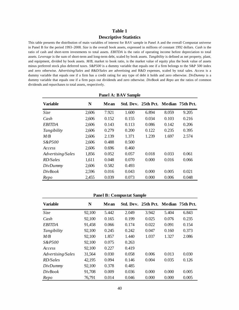
40

Table 1

Descriptive Statistics This table presents the distribution of main variables of interest for BAV sample in Panel A and the overall Compustat universe

in Panel B for the period 1993–2008. Size is the overall book assets, expressed in millions of constant 1992 dollars. Cash is the

ratio of cash and short-term investments to total assets. EBITDA is the ratio of operating income before depreciation to total

assets. Leverage is the sum of short-term and long-term debt, scaled by book assets. Tangibility is defined as net property, plant,

and equipment, divided by book assets. M/B, market to book ratio, is the market value of equity plus the book value of assets

minus preferred stock plus deferred taxes. S&P500 is a dummy variable that equals one if a firm belongs to the S&P 500 index

and zero otherwise. Advertising/Sales and R&D/Sales are advertising and R&D expenses, scaled by total sales. Access is a

dummy variable that equals one if a firm has a credit rating for any type of debt it holds and zero otherwise. DivDummy is a

dummy variable that equals one if a firm pays out dividends and zero otherwise. DivBook and Repo are the ratios of common

dividends and repurchases to total assets, respectively.

Variable N Mean Std. Dev. 25th Pct. Median 75th Pct.

Size 2,606 7.921 1.600 6.894 8.059 9.205

Cash 2,606 0.152 0.155 0.034 0.103 0.216

EBITDA 2,606 0.143 0.113 0.086 0.142 0.206

Tangibility 2,606 0.279 0.200 0.122 0.235 0.395

M/B 2,606 2.139 1.371 1.239 1.697 2.574

S&P500 2,606 0.488 0.500

Access 2,606 0.696 0.460

Advertising/Sales 1,856 0.052 0.057 0.018 0.033 0.061

RD/Sales 1,611 0.048 0.070 0.000 0.016 0.066

DivDummy 2,606 0.582 0.493

DivBook 2,596 0.016 0.043 0.000 0.005 0.021

Repo 2,455 0.039 0.073 0.000 0.006 0.048

Variable N Mean Std. Dev. 25th Pct. Median 75th Pct.

Size 92,100 5.442 2.049 3.942 5.404 6.843

Cash 92,100 0.165 0.199 0.025 0.076 0.235

EBITDA 91,458 0.066 0.174 0.022 0.091 0.154

Tangibility 92,100 0.245 0.242 0.047 0.160 0.373

M/B 92,100 1.857 1.440 1.037 1.327 2.086

S&P500 92,100 0.075 0.263

Access 92,100 0.227 0.419

Advertising/Sales 31,564 0.030 0.058 0.006 0.013 0.030

RD/Sales 42,195 0.094 0.146 0.004 0.035 0.126

DivDummy 92,100 0.378 0.485

DivBook 91,708 0.009 0.036 0.000 0.000 0.005

Repo 76,791 0.014 0.046 0.000 0.000 0.005

Panel A: BAV Sample

Panel B: Compustat Sample

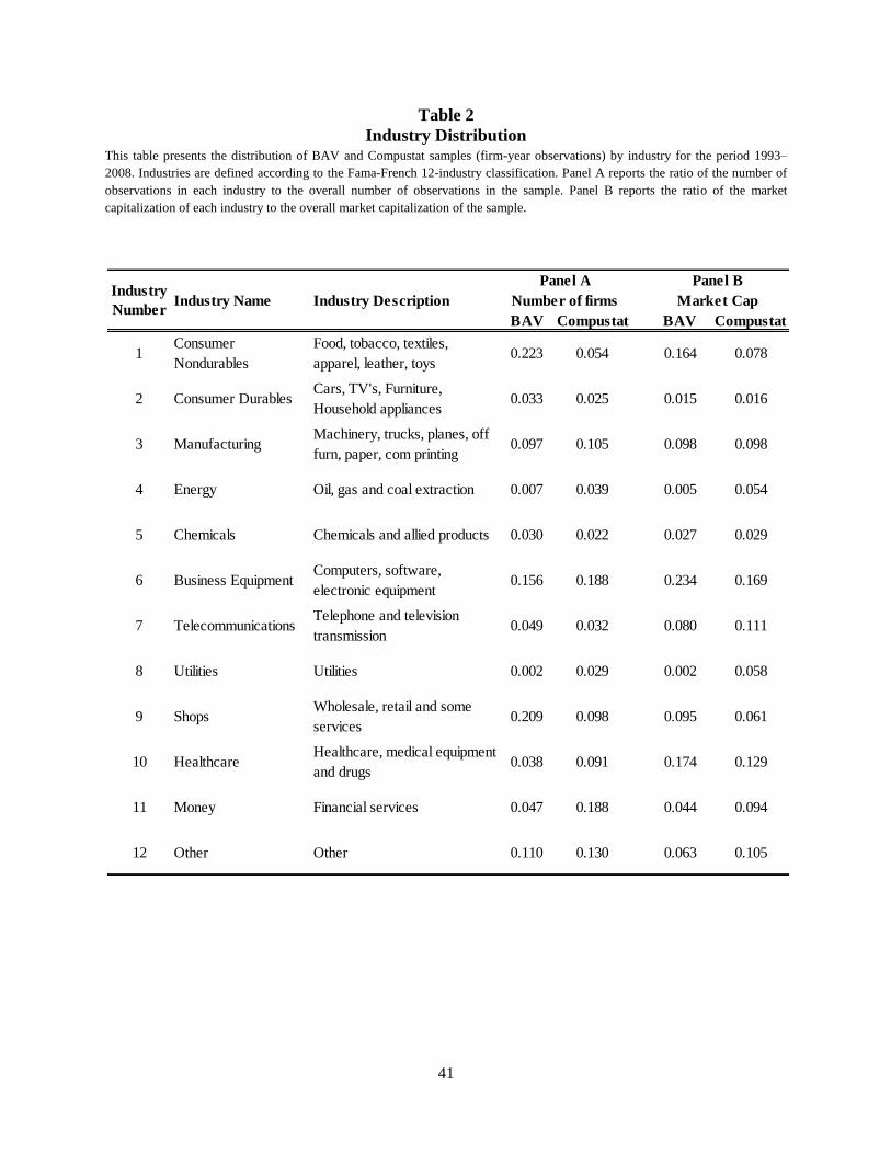
41

Table 2

Industry Distribution This table presents the distribution of BAV and Compustat samples (firm-year observations) by industry for the period 1993–

2008. Industries are defined according to the Fama-French 12-industry classification. Panel A reports the ratio of the number of

observations in each industry to the overall number of observations in the sample. Panel B reports the ratio of the market

capitalization of each industry to the overall market capitalization of the sample.

Industry Name Industry Description

BAV Compustat BAV Compustat

1Consumer

Nondurables

Food, tobacco, textiles,

apparel, leather, toys0.223 0.054 0.164 0.078

2 Consumer DurablesCars, TV's, Furniture,

Household appliances0.033 0.025 0.015 0.016

3 ManufacturingMachinery, trucks, planes, off

furn, paper, com printing0.097 0.105 0.098 0.098

4 Energy Oil, gas and coal extraction 0.007 0.039 0.005 0.054

5 Chemicals Chemicals and allied products 0.030 0.022 0.027 0.029

6 Business EquipmentComputers, software,

electronic equipment0.156 0.188 0.234 0.169

7 TelecommunicationsTelephone and television

transmission0.049 0.032 0.080 0.111

8 Utilities Utilities 0.002 0.029 0.002 0.058

9 ShopsWholesale, retail and some

services0.209 0.098 0.095 0.061

10 HealthcareHealthcare, medical equipment

and drugs0.038 0.091 0.174 0.129

11 Money Financial services 0.047 0.188 0.044 0.094

12 Other Other 0.110 0.130 0.063 0.105

Panel A Panel BIndustry

NumberNumber of firms Market Cap

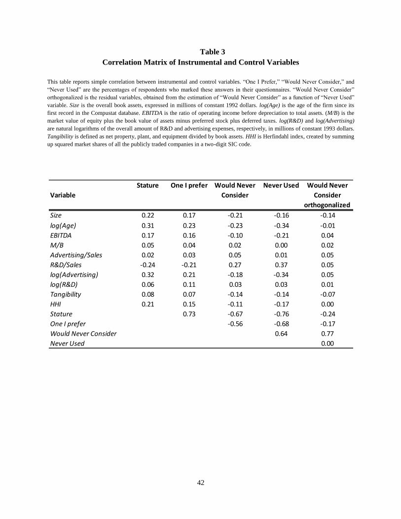
42

Table 3

Correlation Matrix of Instrumental and Control Variables

This table reports simple correlation between instrumental and control variables. ―One I Prefer,‖ ―Would Never Consider,‖ and

―Never Used‖ are the percentages of respondents who marked these answers in their questionnaires. ―Would Never Consider‖

orthogonalized is the residual variables, obtained from the estimation of ―Would Never Consider‖ as a function of ―Never Used‖

variable. Size is the overall book assets, expressed in millions of constant 1992 dollars. log(Age) is the age of the firm since its

first record in the Compustat database. EBITDA is the ratio of operating income before depreciation to total assets. (M/B) is the

market value of equity plus the book value of assets minus preferred stock plus deferred taxes. log(R&D) and log(Advertising)

are natural logarithms of the overall amount of R&D and advertising expenses, respectively, in millions of constant 1993 dollars.

Tangibility is defined as net property, plant, and equipment divided by book assets. HHI is Herfindahl index, created by summing

up squared market shares of all the publicly traded companies in a two-digit SIC code.

Variable

Stature One I prefer Would Never

Consider

Never Used Would Never

Consider

orthogonalized

Size 0.22 0.17 -0.21 -0.16 -0.14

log(Age) 0.31 0.23 -0.23 -0.34 -0.01

EBITDA 0.17 0.16 -0.10 -0.21 0.04

M/B 0.05 0.04 0.02 0.00 0.02

Advertising/Sales 0.02 0.03 0.05 0.01 0.05

R&D/Sales -0.24 -0.21 0.27 0.37 0.05

log(Advertising) 0.32 0.21 -0.18 -0.34 0.05

log(R&D) 0.06 0.11 0.03 0.03 0.01

Tangibility 0.08 0.07 -0.14 -0.14 -0.07

HHI 0.21 0.15 -0.11 -0.17 0.00

Stature 0.73 -0.67 -0.76 -0.24

One I prefer -0.56 -0.68 -0.17

Would Never Consider 0.64 0.77

Never Used 0.00

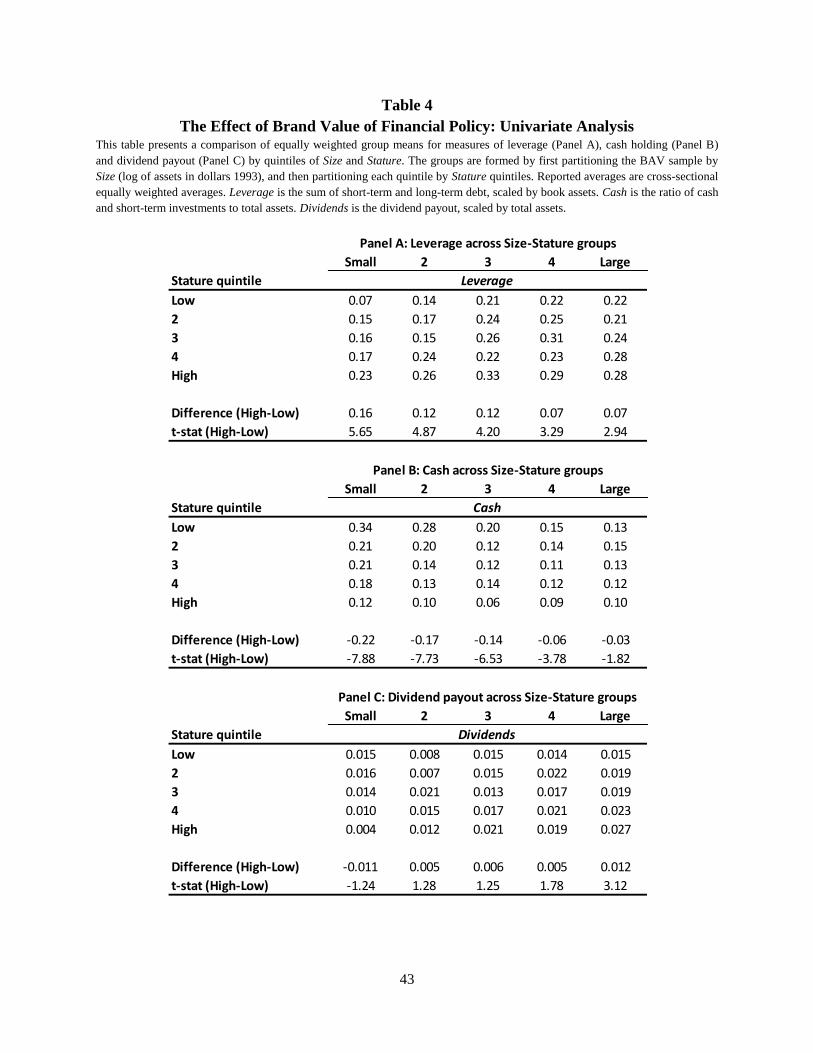
43

Table 4

The Effect of Brand Value of Financial Policy: Univariate Analysis This table presents a comparison of equally weighted group means for measures of leverage (Panel A), cash holding (Panel B)

and dividend payout (Panel C) by quintiles of Size and Stature. The groups are formed by first partitioning the BAV sample by

Size (log of assets in dollars 1993), and then partitioning each quintile by Stature quintiles. Reported averages are cross-sectional

equally weighted averages. Leverage is the sum of short-term and long-term debt, scaled by book assets. Cash is the ratio of cash

and short-term investments to total assets. Dividends is the dividend payout, scaled by total assets.

Small 2 3 4 Large

Stature quintile

Low 0.07 0.14 0.21 0.22 0.22

2 0.15 0.17 0.24 0.25 0.21

3 0.16 0.15 0.26 0.31 0.24

4 0.17 0.24 0.22 0.23 0.28

High 0.23 0.26 0.33 0.29 0.28

Difference (High-Low) 0.16 0.12 0.12 0.07 0.07

t-stat (High-Low) 5.65 4.87 4.20 3.29 2.94

Small 2 3 4 Large

Stature quintile

Low 0.34 0.28 0.20 0.15 0.13

2 0.21 0.20 0.12 0.14 0.15

3 0.21 0.14 0.12 0.11 0.13

4 0.18 0.13 0.14 0.12 0.12

High 0.12 0.10 0.06 0.09 0.10

Difference (High-Low) -0.22 -0.17 -0.14 -0.06 -0.03

t-stat (High-Low) -7.88 -7.73 -6.53 -3.78 -1.82

Small 2 3 4 Large

Stature quintile

Low 0.015 0.008 0.015 0.014 0.015

2 0.016 0.007 0.015 0.022 0.019

3 0.014 0.021 0.013 0.017 0.019

4 0.010 0.015 0.017 0.021 0.023

High 0.004 0.012 0.021 0.019 0.027

Difference (High-Low) -0.011 0.005 0.006 0.005 0.012

t-stat (High-Low) -1.24 1.28 1.25 1.78 3.12

Leverage

Panel A: Leverage across Size-Stature groups

Panel B: Cash across Size-Stature groups

Cash

Panel C: Dividend payout across Size-Stature groups

Dividends

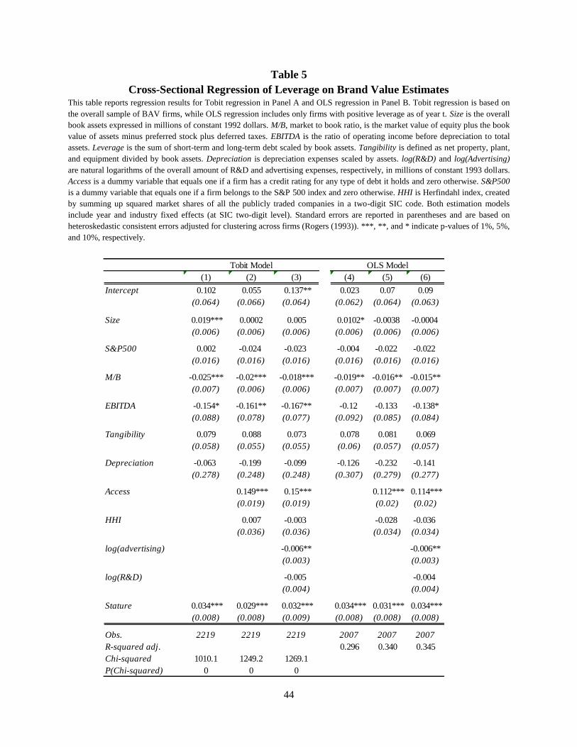
44

Table 5

Cross-Sectional Regression of Leverage on Brand Value Estimates This table reports regression results for Tobit regression in Panel A and OLS regression in Panel B. Tobit regression is based on

the overall sample of BAV firms, while OLS regression includes only firms with positive leverage as of year t. Size is the overall

book assets expressed in millions of constant 1992 dollars. M/B, market to book ratio, is the market value of equity plus the book

value of assets minus preferred stock plus deferred taxes. EBITDA is the ratio of operating income before depreciation to total

assets. Leverage is the sum of short-term and long-term debt scaled by book assets. Tangibility is defined as net property, plant,

and equipment divided by book assets. Depreciation is depreciation expenses scaled by assets. log(R&D) and log(Advertising)

are natural logarithms of the overall amount of R&D and advertising expenses, respectively, in millions of constant 1993 dollars.

Access is a dummy variable that equals one if a firm has a credit rating for any type of debt it holds and zero otherwise. S&P500

is a dummy variable that equals one if a firm belongs to the S&P 500 index and zero otherwise. HHI is Herfindahl index, created

by summing up squared market shares of all the publicly traded companies in a two-digit SIC code. Both estimation models

include year and industry fixed effects (at SIC two-digit level). Standard errors are reported in parentheses and are based on

heteroskedastic consistent errors adjusted for clustering across firms (Rogers (1993)). ***, **, and * indicate p-values of 1%, 5%,

and 10%, respectively.

(1) (2) (3) (4) (5) (6)

Intercept 0.102 0.055 0.137** 0.023 0.07 0.09

(0.064) (0.066) (0.064) (0.062) (0.064) (0.063)

Size 0.019*** 0.0002 0.005 0.0102* -0.0038 -0.0004

(0.006) (0.006) (0.006) (0.006) (0.006) (0.006)

S&P500 0.002 -0.024 -0.023 -0.004 -0.022 -0.022

(0.016) (0.016) (0.016) (0.016) (0.016) (0.016)

M/B -0.025*** -0.02*** -0.018*** -0.019** -0.016** -0.015**

(0.007) (0.006) (0.006) (0.007) (0.007) (0.007)

EBITDA -0.154* -0.161** -0.167** -0.12 -0.133 -0.138*

(0.088) (0.078) (0.077) (0.092) (0.085) (0.084)

Tangibility 0.079 0.088 0.073 0.078 0.081 0.069

(0.058) (0.055) (0.055) (0.06) (0.057) (0.057)

Depreciation -0.063 -0.199 -0.099 -0.126 -0.232 -0.141

(0.278) (0.248) (0.248) (0.307) (0.279) (0.277)

Access 0.149*** 0.15*** 0.112*** 0.114***

(0.019) (0.019) (0.02) (0.02)

HHI 0.007 -0.003 -0.028 -0.036

(0.036) (0.036) (0.034) (0.034)

log(advertising) -0.006** -0.006**

(0.003) (0.003)

log(R&D) -0.005 -0.004

(0.004) (0.004)

Stature 0.034*** 0.029*** 0.032*** 0.034*** 0.031*** 0.034***

(0.008) (0.008) (0.009) (0.008) (0.008) (0.008)

Obs. 2219 2219 2219 2007 2007 2007

R-squared adj. 0.296 0.340 0.345

Chi-squared 1010.1 1249.2 1269.1

P(Chi-squared) 0 0 0

Tobit Model OLS Model

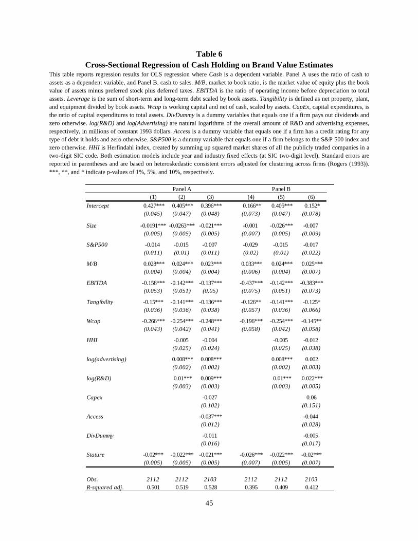
45

Table 6

Cross-Sectional Regression of Cash Holding on Brand Value Estimates This table reports regression results for OLS regression where Cash is a dependent variable. Panel A uses the ratio of cash to

assets as a dependent variable, and Panel B, cash to sales. M/B, market to book ratio, is the market value of equity plus the book

value of assets minus preferred stock plus deferred taxes. EBITDA is the ratio of operating income before depreciation to total

assets. Leverage is the sum of short-term and long-term debt scaled by book assets. Tangibility is defined as net property, plant,

and equipment divided by book assets. Wcap is working capital and net of cash, scaled by assets. CapEx, capital expenditures, is

the ratio of capital expenditures to total assets. DivDummy is a dummy variables that equals one if a firm pays out dividends and

zero otherwise. log(R&D) and log(Advertising) are natural logarithms of the overall amount of R&D and advertising expenses,

respectively, in millions of constant 1993 dollars. Access is a dummy variable that equals one if a firm has a credit rating for any

type of debt it holds and zero otherwise. S&P500 is a dummy variable that equals one if a firm belongs to the S&P 500 index and

zero otherwise. HHI is Herfindahl index, created by summing up squared market shares of all the publicly traded companies in a

two-digit SIC code. Both estimation models include year and industry fixed effects (at SIC two-digit level). Standard errors are

reported in parentheses and are based on heteroskedastic consistent errors adjusted for clustering across firms (Rogers (1993)).

***, **, and * indicate p-values of 1%, 5%, and 10%, respectively.

(1) (2) (3) (4) (5) (6)

Intercept 0.427*** 0.405*** 0.396*** 0.166** 0.405*** 0.152*

(0.045) (0.047) (0.048) (0.073) (0.047) (0.078)

Size -0.0191*** -0.0263*** -0.021*** -0.001 -0.026*** -0.007

(0.005) (0.005) (0.005) (0.007) (0.005) (0.009)

S&P500 -0.014 -0.015 -0.007 -0.029 -0.015 -0.017

(0.011) (0.01) (0.011) (0.02) (0.01) (0.022)

M/B 0.028*** 0.024*** 0.023*** 0.033*** 0.024*** 0.025***

(0.004) (0.004) (0.004) (0.006) (0.004) (0.007)

EBITDA -0.158*** -0.142*** -0.137*** -0.437*** -0.142*** -0.383***

(0.053) (0.051) (0.05) (0.075) (0.051) (0.073)

Tangibility -0.15*** -0.141*** -0.136*** -0.126** -0.141*** -0.125*

(0.036) (0.036) (0.038) (0.057) (0.036) (0.066)

Wcap -0.266*** -0.254*** -0.248*** -0.196*** -0.254*** -0.145**

(0.043) (0.042) (0.041) (0.058) (0.042) (0.058)

HHI -0.005 -0.004 -0.005 -0.012

(0.025) (0.024) (0.025) (0.038)

log(advertising) 0.008*** 0.008*** 0.008*** 0.002

(0.002) (0.002) (0.002) (0.003)

log(R&D) 0.01*** 0.009*** 0.01*** 0.022***

(0.003) (0.003) (0.003) (0.005)

Capex -0.027 0.06

(0.102) (0.151)

Access -0.037*** -0.044

(0.012) (0.028)

DivDummy -0.011 -0.005

(0.016) (0.017)

Stature -0.02*** -0.022*** -0.021*** -0.026*** -0.022*** -0.02***

(0.005) (0.005) (0.005) (0.007) (0.005) (0.007)

Obs. 2112 2112 2103 2112 2112 2103

R-squared adj. 0.501 0.519 0.528 0.395 0.409 0.412

Panel BPanel A

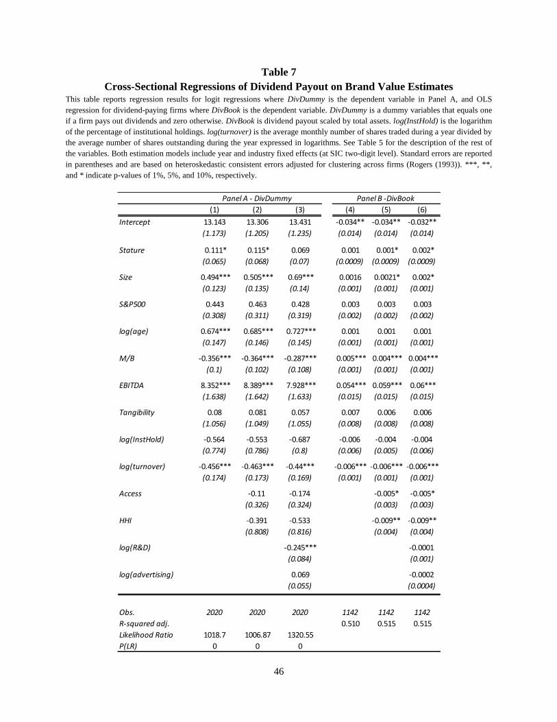
46

Table 7

Cross-Sectional Regressions of Dividend Payout on Brand Value Estimates This table reports regression results for logit regressions where DivDummy is the dependent variable in Panel A, and OLS

regression for dividend-paying firms where DivBook is the dependent variable. DivDummy is a dummy variables that equals one

if a firm pays out dividends and zero otherwise. DivBook is dividend payout scaled by total assets. log(InstHold) is the logarithm

of the percentage of institutional holdings. log(turnover) is the average monthly number of shares traded during a year divided by

the average number of shares outstanding during the year expressed in logarithms. See Table 5 for the description of the rest of

the variables. Both estimation models include year and industry fixed effects (at SIC two-digit level). Standard errors are reported

in parentheses and are based on heteroskedastic consistent errors adjusted for clustering across firms (Rogers (1993)). ***, **,

and * indicate p-values of 1%, 5%, and 10%, respectively.

(1) (2) (3) (4) (5) (6)

Intercept 13.143 13.306 13.431 -0.034** -0.034** -0.032**

(1.173) (1.205) (1.235) (0.014) (0.014) (0.014)

Stature 0.111* 0.115* 0.069 0.001 0.001* 0.002*

(0.065) (0.068) (0.07) (0.0009) (0.0009) (0.0009)

Size 0.494*** 0.505*** 0.69*** 0.0016 0.0021* 0.002*

(0.123) (0.135) (0.14) (0.001) (0.001) (0.001)

S&P500 0.443 0.463 0.428 0.003 0.003 0.003

(0.308) (0.311) (0.319) (0.002) (0.002) (0.002)

log(age) 0.674*** 0.685*** 0.727*** 0.001 0.001 0.001

(0.147) (0.146) (0.145) (0.001) (0.001) (0.001)

M/B -0.356*** -0.364*** -0.287*** 0.005*** 0.004*** 0.004***

(0.1) (0.102) (0.108) (0.001) (0.001) (0.001)

EBITDA 8.352*** 8.389*** 7.928*** 0.054*** 0.059*** 0.06***

(1.638) (1.642) (1.633) (0.015) (0.015) (0.015)

Tangibility 0.08 0.081 0.057 0.007 0.006 0.006

(1.056) (1.049) (1.055) (0.008) (0.008) (0.008)

log(InstHold) -0.564 -0.553 -0.687 -0.006 -0.004 -0.004

(0.774) (0.786) (0.8) (0.006) (0.005) (0.006)

log(turnover) -0.456*** -0.463*** -0.44*** -0.006*** -0.006*** -0.006***

(0.174) (0.173) (0.169) (0.001) (0.001) (0.001)

Access -0.11 -0.174 -0.005* -0.005*

(0.326) (0.324) (0.003) (0.003)

HHI -0.391 -0.533 -0.009** -0.009**

(0.808) (0.816) (0.004) (0.004)

log(R&D) -0.245*** -0.0001

(0.084) (0.001)

log(advertising) 0.069 -0.0002

(0.055) (0.0004)

Obs. 2020 2020 2020 1142 1142 1142

R-squared adj. 0.510 0.515 0.515

Likelihood Ratio 1018.7 1006.87 1320.55

P(LR) 0 0 0

Panel A - DivDummy Panel B -DivBook

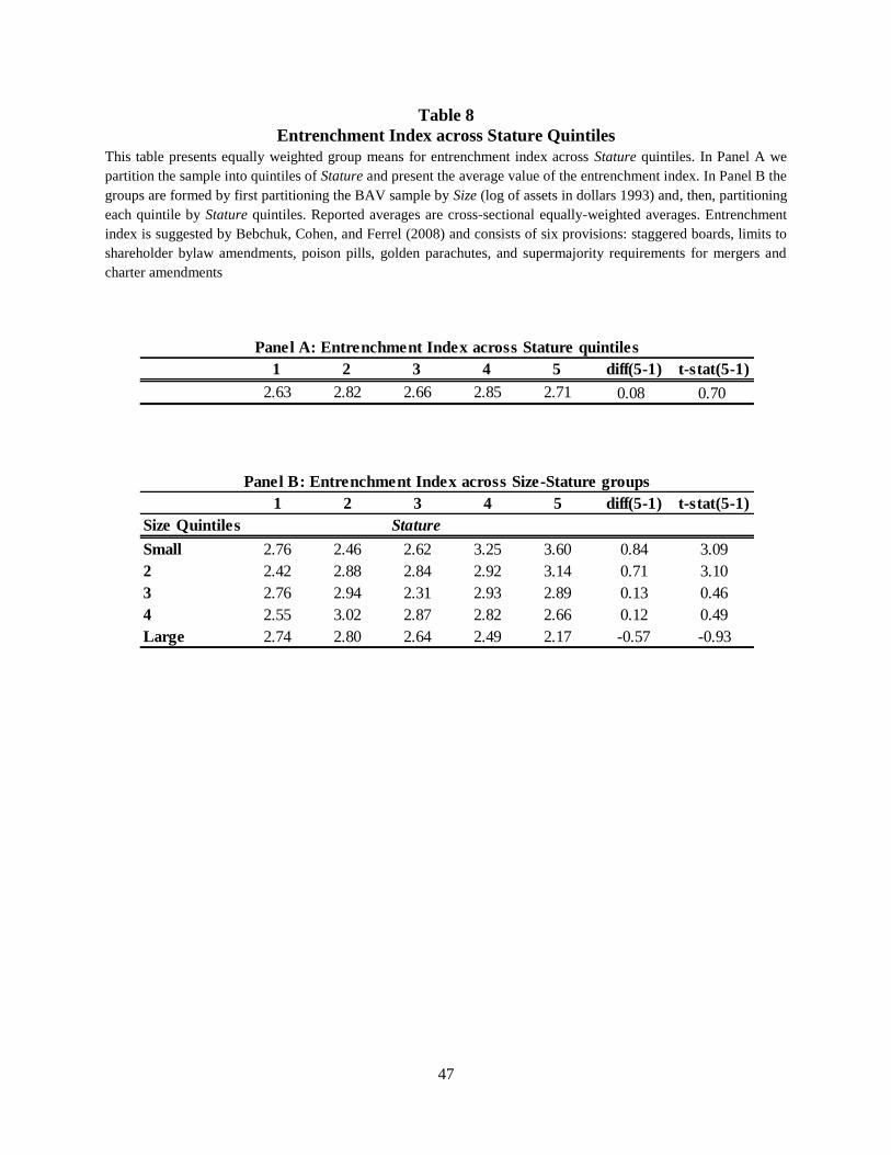
47

Table 8

Entrenchment Index across Stature Quintiles

This table presents equally weighted group means for entrenchment index across Stature quintiles. In Panel A we

partition the sample into quintiles of Stature and present the average value of the entrenchment index. In Panel B the

groups are formed by first partitioning the BAV sample by Size (log of assets in dollars 1993) and, then, partitioning

each quintile by Stature quintiles. Reported averages are cross-sectional equally-weighted averages. Entrenchment

index is suggested by Bebchuk, Cohen, and Ferrel (2008) and consists of six provisions: staggered boards, limits to

shareholder bylaw amendments, poison pills, golden parachutes, and supermajority requirements for mergers and

charter amendments

1 2 3 4 5 diff(5-1) t-stat(5-1)

2.63 2.82 2.66 2.85 2.71 0.08 0.70

1 2 3 4 5 diff(5-1) t-stat(5-1)

Size Quintiles

Small 2.76 2.46 2.62 3.25 3.60 0.84 3.09

2 2.42 2.88 2.84 2.92 3.14 0.71 3.10

3 2.76 2.94 2.31 2.93 2.89 0.13 0.46

4 2.55 3.02 2.87 2.82 2.66 0.12 0.49

Large 2.74 2.80 2.64 2.49 2.17 -0.57 -0.93

Stature

Panel B: Entrenchment Index across Size-Stature groups

Panel A: Entrenchment Index across Stature quintiles

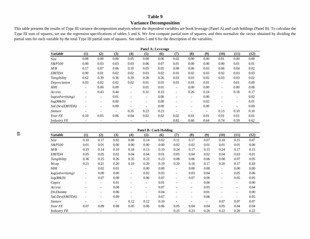
48

Table 9

Variance Decomposition

This table presents the results of Type III variance decomposition analysis where the dependent variables are book leverage (Panel A) and cash holdings (Panel B). To calculate the

Type III sum of squares, we use the regression specifications of tables 5 and 6. We first compute partial sum of squares, and then normalize the vector obtained by dividing the

partial sum for each variable by the total Type III partial sum of squares. See tables 5 and 6 for the description of the variables.

.

Variable (1) (2) (3) (4) (5) (6) (7) (8) (9) (10) (11) (12)

Size 0.08 0.00 0.00 0.05 0.00 0.00 0.02 0.00 0.00 0.01 0.00 0.00

S&P500 0.00 0.03 0.03 0.03 0.06 0.07 0.01 0.00 0.00 0.00 0.01 0.01

M/B 0.17 0.07 0.06 0.10 0.05 0.05 0.08 0.06 0.03 0.06 0.04 0.02

EBITDA 0.00 0.01 0.02 0.02 0.03 0.02 0.01 0.02 0.03 0.02 0.03 0.03

Tangibility 0.62 0.39 0.36 0.39 0.28 0.26 0.03 0.03 0.02 0.03 0.03 0.02

Depreciation 0.03 0.02 0.02 0.02 0.01 0.01 0.01 0.01 0.01 - 0.01 0.00

HHI - 0.00 0.00 - 0.01 0.01 - 0.00 0.00 - 0.00 0.00

Access - 0.43 0.44 - 0.31 0.33 - 0.26 0.24 - 0.18 0.17

log(advertising) - - 0.01 - - 0.00 - - 0.00 - - 0.02

log(R&D) - - 0.00 - - 0.00 - - 0.02 - - 0.01

Std.Dev(EBITDA) - - 0.00 - - 0.00 - - 0.00 - - 0.00

Stature - - - 0.35 0.23 0.23 - - - 0.13 0.10 0.10

Year FE 0.10 0.05 0.06 0.04 0.02 0.02 0.02 0.01 0.01 0.01 0.01 0.01

Industry FE - - - - - - 0.82 0.60 0.64 0.74 0.59 0.62

Variable (1) (2) (3) (4) (5) (6) (7) (8) (9) (10) (11) (12)

Size 0.10 0.17 0.02 0.08 0.14 0.02 0.11 0.17 0.07 0.10 0.15 0.07

S&P500 0.01 0.01 0.00 0.00 0.00 0.00 0.02 0.02 0.01 0.01 0.01 0.00

M/B 0.19 0.14 0.10 0.18 0.13 0.10 0.24 0.17 0.15 0.24 0.17 0.15

EBITDA 0.05 0.05 0.02 0.04 0.04 0.01 0.05 0.04 0.02 0.04 0.03 0.01

Tangibility 0.36 0.25 0.26 0.35 0.23 0.23 0.08 0.06 0.06 0.08 0.07 0.05

Wcap 0.21 0.21 0.20 0.19 0.20 0.19 0.20 0.16 0.17 0.20 0.17 0.18

HHI - 0.02 0.01 - 0.00 0.00 - 0.00 0.00 - 0.00 0.00

log(advertising) - 0.00 0.00 - 0.02 0.03 - 0.03 0.04 - 0.05 0.06

log(R&D) - 0.07 0.08 - 0.06 0.07 - 0.07 0.06 - 0.05 0.05

Capex - - 0.01 - - 0.01 - - 0.00 - - 0.00

Access - - 0.08 - - 0.07 - - 0.05 - - 0.04

DivDummy - - 0.06 - - 0.04 - - 0.01 - - 0.00

Std.Dev(EBITDA) - - 0.09 - - 0.07 - - 0.06 - - 0.05

Stature - - - 0.12 0.12 0.10 - - - 0.07 0.07 0.07

Year FE 0.07 0.09 0.08 0.05 0.06 0.06 0.05 0.04 0.04 0.05 0.04 0.04

Industry FE - - - - - - 0.25 0.23 0.26 0.22 0.20 0.22

Panel A: Leverage

Panel B: Cash Holding48

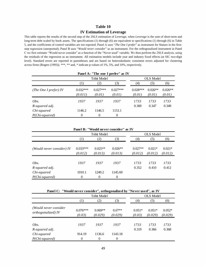
49

Table 10

IV Estimation of Leverage This table reports the results of the second step of the 2SLS estimation of Leverage, when Leverage is the sum of short-term and

long-term debt scaled by book assets. The specifications (1) through (6) are equivalent to specifications (1) through (6) in Table

5, and the coefficients of control variables are not reported. Panel A uses ―The One I prefer‖ as instrument for Stature in the first-

step regression (unreported); Panel B uses ―Would never consider‖ as an instrument. For the orthogonalized instrument in Panel

C we first estimate ―Would never consider‖ as a function of the ―Never used‖ variable. We then perform the 2SLS analysis, using

the residuals of the regression as an instrument. All estimation models include year and industry fixed effects (at SIC two-digit

level). Standard errors are reported in parentheses and are based on heteroskedastic consistent errors adjusted for clustering

across firms (Rogers (1993)). ***, ** and, * indicate p-values of 1%, 5%, and 10%, respectively.

(1) (2) (3) (4) (5) (6)

(The One I prefer) IV 0.032*** 0.027*** 0.027*** 0.028*** 0.026** 0.026**

(0.011) (0.01) (0.01) (0.01) (0.01) (0.01)

Obs. 1937 1937 1937 1733 1733 1733

R-squared adj. 0.300 0.347 0.349

Chi-squared 1146.2 1146.5 1153.1

P(Chi-squared) 0 0 0

(1) (2) (3) (4) (5) (6)

(Would never consider) IV 0.033*** 0.025** 0.026** 0.027** 0.021* 0.021*

(0.012) (0.013) (0.013) (0.012) (0.012) (0.012)

Obs. 1937 1937 1937 1733 1733 1733

R-squared adj. 0.352 0.410 0.412

Chi-squared 1010.1 1249.2 1145.69

P(Chi-squared) 0 0 0

(1) (2) (3) (4) (5) (6)

0.076*** 0.069** 0.07** 0.051* 0.051* 0.052*

(0.03) (0.029) (0.029) (0.03) (0.029) (0.029)

Obs. 1937 1937 1937 1733 1733 1733

R-squared adj. 0.319 0.366 0.368

Chi-squared 914.19 1136.6 1143.18

P(Chi-squared) 0 0 0

(Would never consider

orthogonalized) IV

Panel A: "The one I prefer" as IV

Panel B: "Would never consider" as IV

Panel C: "Would never consider", orthogonalized by "Never used", as IV

Tobit Model OLS Model

Tobit Model OLS Model

Tobit Model OLS Model

50

Table 11

IV Estimation of Cash Holding This table reports the results of the second step of the 2SLS estimation of cash, when cash is scaled by book assets in

specifications (1) through (3) and by Sales in specifications (4) through (6). The specifications (1) through (6) are equivalent to

specifications (1) through (6) in Table 6, and the coefficients of control variables are not reported. Panel A uses ―The One I

prefer‖ as instrument for Stature in the first-step regression (unreported); Panel B uses ―Would never consider‖ as an instrument.

For the orthogonalized instrument in Panel C we first estimate ―Would never consider‖ as a function of the ―Never used‖

variable. We then perform the 2SLS analysis, using the residuals of the regression as an instrument. All estimation models

include year and industry fixed effects (at SIC the-digit level). Standard errors are reported in parentheses and are based on

heteroskedastic consistent errors adjusted for clustering across firms (Rogers (1993)). ***, **, and * indicate p-values of 1%, 5%,

and 10%, respectively.

(1) (2) (3) (4) (5) (6)

(The One I prefer) IV -0.028*** -0.027*** -0.026*** -0.033*** -0.031*** -0.029***

(0.006) (0.006) (0.006) (0.01) (0.01) (0.01)

Obs. 1844 1844 1844 1844 1844 1844

R-squared adj. 0.531 0.539 0.546 0.415 0.421 0.422

(1) (2) (3) (4) (5) (6)

(Would never consider) IV -0.027*** -0.027*** -0.024*** -0.042*** -0.039*** -0.038***

(0.008) (0.008) (0.008) (0.012) (0.011) (0.012)

Obs. 1844 1844 1844 1844 1844 1844

R-squared adj. 0.527 0.536 0.542 0.416 0.422 0.423

(1) (2) (3) (4) (5) (6)

-0.044** -0.047*** -0.04** -0.075*** -0.084*** -0.078***

(0.018) (0.018) (0.018) (0.027) (0.028) (0.028)

Obs. 1844 1844 1844 1844 1844 1844

R-squared adj. 0.538 0.547 0.555 0.432 0.440 0.442

(Would never consider

orthogonalized) IV

Panel A: "The one I prefer" as IV

Panel B: "Would never consider" as IV

Panel C: "Would never consider" orthogonalized by "Never used" as IV

Cash/Assets Cash/Sales

Cash/Assets Cash/Sales

Cash/Assets Cash/Sales