1

Production Patterns of Multinational Enterprises: The Knowledge-Capital Model Revisited

Kazuhiko OYAMADA*

July 31, 2015

(Revised March 10, 2016)

Abstract

To prepare an answer to the question of how a developing country can attract FDI, this

paper explored the factors and policies that may help bring FDI into a developing country

by utilizing an extended version of the knowledge-capital model. With a special focus on

the effects of FTA/EPA between a market country and a developing country, simulations

with the model revealed the following: (1) although FTA/EPA generally tends to increase

FDI to a developing country, the possibility to improve welfare through increased demand

for skilled and unskilled labor becomes lower as the size of the country grows; (2) a

developing country may suffer severe welfare losses through FTA/EPA if the availability of

skilled labor is extremely limited; (3) because the additional implementation of cost-saving

policies to reduce the firm-type/trade-link specific fixed cost tends to depreciate the price of

skilled labor by saving its input, a developing country can enhance welfare gains from FTA,

and it is even possible to recover the welfare effects from negative to positive, by making

the arrangement to be EPA.

Keywords: foreign direct investment; multinational enterprise; export platform; complex

integration; free trade agreement; economic partnership agreement

JEL Classification Numbers: F11; F12; F15; F23

* Institute of Developing Economies, Japan External Trade Organization (IDE-JETRO), 3-2-2 Wakaba,

Mihama-Ku, Chiba-Shi, Chiba 261-8545, Japan (kazuhiko_oyamada@ide.go.jp)

2

1. Introduction

How can a developing country attract foreign direct investment (FDI)? This question has

long been the subject of debate among policy-makers in developing economies who regard

FDI as an important catalyst for economic growth. As the global economy has become

increasingly interdependent, multinational enterprises (MNEs) form multilateral production

networks, where production processes are subdivided into several stages and some

developing countries have successfully participated in certain parts of these networks. The

purpose of this paper is to explore the factors and policies that may help to bring FDI into a

developing country.

While research on the activities of MNEs has been conducted widely since the late

1980s, a limited number of studies have comprehensively handled every operational pattern

of MNEs in one model. Especially, the export-platform is not much discussed in the

theoretical studies, even though its importance has been revealed by the empirical side.

Because a low-cost developing country may play an important role as an export-platform,

an analytical model for this study must include this type in addition to the typical

horizontal- and vertical-type MNEs.

One of the most sophisticated studies that consider typical types of MNEs including

export-platforms in the same analytical framework was presented by Ekholm, Forslid, and

Markusen (2007). Using a numerical simulation model, in which two market countries and

one exogenously given developing country are considered, they explored the conditions

under four types of firm strategy while gradually changing two types of costs, one for

trading components and the other for assembling components. However, their model has

only one factor of production, and the non-market country is just assumed to set exogenous

factor pricing in a partial equilibrium framework. Another work that nests every type of

MNE in one model is presented by Ito (2013). Extending the two-region, four-country (two

countries in each region) model developed by Navaretti and Venebles (2004) to include

export-platform, he showed that a reduction in trade costs, either inter-regional or

intra-regional, induces firms to choose export-platform rather than other types. To enable

the theoretical model to yield testable hypotheses for empirical testing, he incorporated only

trade costs abstracting production costs away.

A good candidate for the base of an analytical model that includes both trade and

production costs in a general equilibrium setting is the knowledge-capital model developed

by Markusen (1997) and further extended by Zhang and Markusen (1999). Although

export-platform is not taken into account, the computational model is able to verify effects

3

of changes in firm-type on factor prices in the countries where the MNEs are active. As

employment and labor wages in the host country are important factors MNEs use to decide

on a production strategy, this feature based on the general equilibrium nature of the

knowledge-capital model is essential for our study. Thus, we utilized an extended version of

the model for this study.

The remainder of this paper is organized as follows. Section 2 illustrates the structure

and main assumptions of the analytical model. Section 3 explains how the model is

parameterized as a numerical model. In Section 4, we perform simulations and report on the

results that reveal conditions for which each type of firms would be active in a given

economic environment with a special focus on the effects of trade liberalization and

optional cost-saving policies. Finally, Section 5 presents the conclusions of this paper.

2. The Extended Knowledge-Capital Model

The model used in this study is a simple extension of the knowledge-capital model that was

used as the workhorse in Markusen (2002), including national enterprises (NEs), horizontal

MNEs (HMNEs), vertical MNEs (VMNEs), horizontal export-platforms (HEPs), vertical

export-platforms (VEPs), and complexly integrated MNEs (CMNEs). The complex

integration strategy, which was introduced by Yeaple (2003) and studied by Grossman,

Helpman, and Szeidl (2006), is a combination of the horizontal integration for a foreign

market so as to reduce trade costs and the vertical export-platform for the home market to

reduce production costs. The model is also extended to include two developing countries, in

which the final assembly process of multinational production may take place while the

finished products are not sold locally but exported, which is in addition to the original

assumption of two developed countries in which MNEs are established and there are

markets for the commodity produced by those MNEs.1

An important point here is that we do not limit the volumes of those developing

(non-market) countries, which always stay small in terms of factor endowments. Because

the knowledge-capital model is a general equilibrium model, branching out and setting up

subsidiaries by MNEs in a non-market country affects the local factor prices. If the host

country is relatively small, factor prices appreciate more than they would in a relatively 1 While we mainly regard developed and developing countries respectively correspond to market and

non-market countries in this paper, we do not exclude the possibility that a developing country is considered as a market. For example, China could be considered as both final market and non-market production-platform depending on one’s research interest.

4

large country. This may substantially frustrate the incentive of the MNE to stay in the

country and trigger it to find another place where cheaper production factors are available.

With this model, we investigate which production pattern is adopted by firms

established in two countries out of four to sell product in both home and foreign (target)

markets under certain economic circumstances.

2.1 Environment

There are four countries , , , and , indexed as . and are assumed to be

countries in which MNEs are established and there are markets for the commodity

produced by those MNEs. We index these countries or as a subset of . and

are countries in which the final assembly process of multinational productions may take

place while the finished products are not sold locally but exported. The index of these

countries is , another subset of .

There are three types of goods, , , and . The intermediate good (a component)

is used to produce the final product by the MNE. This sector exhibits increasing

returns to scale (IRTS) so that the market is assumed to be imperfectly competitive. is

produced only in the home of the MNE, country , and is sent to country where the final

assembly process takes place. The finished product is sold on the target market . Note

that all MNEs in each production type, national , horizontal , vertical , horizontal

export-platform , vertical export-platform , and complex integration , indexed as

, share identical technologies and productivities. On the other hand, is a regular

product based on a constant-returns-to-scale (CRTS) technology so that the market is

perfectly competitive. is produced in every country , and is sold on the international

market as a perfect substitute.

Production factors are of two types, and , which are immobile among national

boundaries. Although we mainly regard as skilled labor (human capital) in this study, it

can be further extended to include the status of institutions (rules and regulations) and/or

the business environment. is unskilled labor. The national endowments of these factors

are set exogenously in the model. In the experimental simulations, we change the relative

factor endowments for either the market- or non-market-country groups given absolute

levels of total endowments for the groups.

In the IRTS sector, two types of fixed cost, and , are required to start operating

a firm. Whereas , measured in units of unskilled labor , is needed to set up an assembly

plant in country (country specific), , measured in units of skilled labor , is required

5

to establish a firm and its local subsidiary in a foreign country (firm-type/trade-link

specific).

There are also trade costs for international transport of and , which are specific

to each trade link. We assume that unskilled labor in the exporting country is used for

this. On the other hand, it is assumed for simplicity that shipping does not generate any

cost.

2.2 Type-Y Good Producer

There are two groups of firms producing , one is established and headquartered in

country and the other in (country ). The markets for are limited to countries

and (country ). Good is produced in two stages with IRTS technology by

imperfectly competitive firms. In the first stage, each firm produces its components

(intermediate good) only in its home country using skilled labor . In the second stage,

a firm may send its components to domestic and/or foreign subsidiary(ies) and finalize the

production of there, assembling components using locally hired unskilled labor .

This assembly process can take place in any country . If the assembly is taking place in a

non-market country , all of the final products are exported to one or both of the market

countries . If it is performed in the home country , the products are sold domestically

and/or exported to a foreign market . If it takes place in a foreign market country , the

products are sold locally and/or exported back to the home market .

There are both firm-level and plant-level scale economies. By free entry and exit of

firms in each operational pattern, a production regime, which refers to a combination of

firm types in an equilibrium, is determined. Following Ekholm, Forslid, and Markusen

(2007), regimes will be denoted by suffices with letters, the first letter referring to a firm’s

home country , the second one referring to the destination market , and the third one

referring to the location of its assembly plant ( or ). When it is possible to omit some of

those letters without creating any confusion, the length of the suffix becomes shorter. The

regimes are categorized into six types, , , , , , and , which express the

production pattern of a firm. The six production types are defined as follows.

Type-N: NEs that maintain a single plant with headquarters in country . This type of firms

produces both components and final products in country . A fraction of the

products may or may not be exported to country .

6

Type-H: HMNEs that maintain plants in both market countries, with headquarters in

country . This type of firms produces components in country , some of which are

shipped to an assembly plant in country . The final products are produced in both

market countries. No fraction of product may be exported.

Type-V: VMNEs that maintain a single plant in the foreign market country , with

headquarters in country . This type of firm produces components in country , which

are then shipped to the assembly plant in country . A fraction of the products may or

may not be exported back to the home market in country .

Type-EH: HEPs that maintain a plant in one of the non-market countries , in addition to

a plant and headquarters in home country . This type of firms produces components in

country , some of which are shipped to an assembly plant in country . All of the final

products produced in country are exported to the foreign market in country , while

the ones produced in the home country are sold domestically.

Type-EV: VEPs that maintain a single plant in one of the non-market countries , with

headquarters in country . This type of firm produces components in country , which

are then shipped to the assembly plant in country . All of the final products are

exported to both of the market countries .

Type-CI: CMNEs that maintain plants both in one of the non-market countries and in

the foreign market country , with headquarters in country . This type of firm produces

components in country , which are then shipped to the assembly plant in countries

and All of the final products produced in country are exported back to the home

market in country , while the ones produced in the foreign market country are sold locally.

Figure 1 shows schematic images of these six types of production patterns. In each

pattern, the headquarters of the firm is located in the country placed on the left-hand side of

the image.

7

Figure 1: Six Types of Production Patterns

2.2.1 Type-N Firm Established in Country

A type-N firm produces three types of products: components ; final products for the

domestic market ; and final products for the foreign market . The skilled

labor requirements to produce one unit of a component in home country can be

expressed as:

, (1)

where

is the skilled labor input hired in country ;

is the quantity of components produced;

is the fixed cost to establish a NE in country ; and

is the unit input requirement for skilled labor.

Similarly, the requirements for both unskilled labor and components to produce one unit of

final product in home country can be expressed as:

∑ ; (2)

8

and

∑ , (3)

where

is the unskilled labor hired in country ;

is the quantity of final products;

is the fixed cost to set up an assembly plant in country ;

is the unit input requirement for unskilled labor;

is the unit input requirement for components; and

is the rate of transportation margin on final products.

Then, the cost function for a type-N firm is given by:

1

, (4)

where

is the price of skilled labor;

is the price of unskilled labor; and

is the rate of import tariff on final products.

The first term on the right-hand side of Equation (4) corresponds to the variable cost with

respect to . Similarly, the second term corresponds to the one with respect to

. The last term corresponds to the total fixed cost.

2.2.2 Type-H Firm Established in Country

A type-H firm produces four types of products: components ; components ;

final products for the domestic market ; and final products for the foreign market

. The skilled labor requirements to produce one unit of components in the home

country can be expressed as:

∑ , (5)

where

is the skilled labor input hired in country ;

is the quantity of components produced; and

is the fixed cost to establish a HMNE in country .

9

To ship components from country to destination , the following amount of

unskilled labor must be hired in country :

, (6)

where

is the unskilled labor hired for international shipping; and

is the rate of transportation margin on components.

Next, the requirements for both unskilled labor and components to produce one unit of final

products in home country can be expressed as:

; (7)

and

, (8)

where

is the unskilled labor input hired in country ; and

is the quantity of final products assembled in country .

Similarly, the requirements for both unskilled labor and components to produce one unit of

final products in the foreign market country are:

; (9)

and

, (10)

where

is the unskilled labor input hired in country ;

is the quantity of final products assembled in country ; and

is the fixed cost to set up an assembly plant in country .

At the local subsidiary in the foreign market country , skilled labor is needed to train

unskilled labor how to handle the intermediate:

, (11)

where

is the skilled labor input hired in country ; and

is the fixed cost to operate an assembly plant in country .

Then, the cost function for a type-H firm is given by:

10

1

∑ , (12)

where

is the rate of import tariff on components.

As in the case of the type-N firm, the first term on the right-hand side of Equation (12)

corresponds to the variable cost with respect to . The second term corresponds to

the one with respect to . The third term is the total fixed cost.

2.2.3 Type-V Firm Established in Country

A type-V firm produces three types of products: components ; final products for the

home market ; and final products for the foreign market . The skilled labor

requirements to produce one unit of components in the home country can be expressed

as:

, (13)

where

is the skilled labor input hired in country ;

is the quantity of components produced; and

is the fixed cost to establish a VMNE in country .

To ship components from country to destination , the following amount of

unskilled labor must be hired in country :

, (14)

where

is the unskilled labor hired for international shipping.

Next, the requirements for both unskilled labor and components to produce one unit of final

products in the foreign market country can be expressed as:

∑ ′′ ; (15)

and

∑ ′′ , (16)

where

is the unskilled labor input hired in country ; and

11

′ is the quantity of final products assembled in country .

Similarly to the case of the type-H firm, skilled labor is needed at the local subsidiary to

train unskilled labor how to handle the intermediate:

, (17)

where

is the skilled labor input hired in country ; and

is the fixed cost to operate an assembly plant in country .

Then, the cost function for a type-V firm is given by:

1 1

1

∑ ∑ . (18)

Note that ′ ′ 0. The first term on the right-hand side of Equation (18) corresponds

to the variable cost with respect to . The second term corresponds to the one with

respect to . The third term is the total fixed cost.

2.2.4 Type-EH Firm Established in Country

A type-EH firm produces four types of products: components ; components ;

final products for the domestic market ; and final products for the foreign market

. The skilled labor requirements to produce one unit of a component in home

country can be expressed as:

, (19)

where

is the skilled labor input hired in country ;

is the quantity of components produced for the domestic plant;

is the quantity of components produced for the plant in country ; and

is the fixed cost to establish a HEP in country .

To ship components from country to a non-market country , the following

amount of unskilled labor must be hired in country :

12

, (20)

where

is the unskilled labor hired for international shipping; and

is the rate of transportation margin on components.

The requirements for both unskilled labor and components to produce one unit of final

products in home country can be expressed as:

; (21)

and

, (22)

where

is the unskilled labor input hired in country ; and

is the quantity of final products assembled in country .

Similarly, the requirements for both unskilled labor and components to produce one unit of

final products in non-market country are:

; (23)

and

, (24)

where

is the unskilled labor input hired in country ;

is the quantity of final products assembled in country for country ;

is the fixed cost to set up an assembly plant in country ; and

is the rate of transportation margin on final products.

At the local subsidiary in non-market country , skilled labor is needed to train unskilled

labor how to handle the intermediate:

, (25)

where

is the skilled labor input hired in country ; and

is the fixed cost to operate an assembly plant in country .

Then, the cost function for a type-EH firm is given by:

1 1

, (26)

13

where

is the rate of import tariff on final products; and

is the rate of import tariff on components.

Note that 0 and 0. The correspondence between the expressions

on the right-hand side of Equation (26) and the variable or fixed cost is the same as before.

2.2.5 Type-EV Firm Established in Country

A type-EV firm produces two types of products: components ; and final products for

market countries . The skilled labor requirements to produce one unit of a component

in home country can be expressed as:

, (27)

where

is the skilled labor input hired in country ;

is the quantity of components produced for the plant in country ; and

is the fixed cost to establish a VEP in country .

To ship components from country to a non-market country , the following

amount of unskilled labor must be hired in country :

, (28)

where

is the unskilled labor hired for international shipping.

The requirements for both unskilled labor and components to produce one unit of final

product in country can be expressed as:

∑ ∑ ; (29)

and

∑ , (30)

where

is the unskilled labor input hired in country ; and

is the quantity of final products assembled in country for country .

As in the previous cases, skilled labor is needed at the local subsidiary to train unskilled

labor how to handle the intermediate:

, (31)

where

is the skilled labor input hired in country ; and

is the fixed cost to operate an assembly plant in country .

14

Then, the cost function for a type-EV firm is given by:

1 1

. (32)

Note that 0. The first term on the right-hand side of Equation (32) corresponds

to the variable cost with respect to , and the second term is the total fixed cost.

2.2.6 Type-CI Firm Established in Country

A type-CI firm produces four types of products: components ; components ;

final products for the domestic market ; and final products for the foreign market

. The skilled labor requirements to produce one unit of a component in home

country can be expressed as:

, (33)

where

is the skilled labor input hired in country ;

is the quantity of components produced for the plant in country ;

is the quantity of components produced for the plant in country ; and

is the fixed cost to establish a CMNE in country .

To ship components and from country to countries and , the

following amount of unskilled labor must be hired in country :

, (34)

where

is the unskilled labor hired for international shipping.

The requirements for both unskilled labor and components to produce one unit of final

products in the foreign market country can be expressed as:

; (35)

and

, (36)

where

is the unskilled labor input hired in country ; and

is the quantity of final products assembled in country for local sales.

Similarly, the requirements for both unskilled labor and components to produce one unit of

final products in non-market country are:

15

; (37)

and

, (38)

where

is the unskilled labor input hired in country ; and

is the quantity of final products assembled in country for country .

At the local subsidiaries in countries and , skilled labor is needed to train unskilled

labor how to handle the intermediate, respectively:

; (39)

and

, (40)

where

is the skilled labor input hired in country ;

is the fixed cost to operate an assembly plant in country .

is the skilled labor input hired in country ; and

is the fixed cost to operate an assembly plant in country .

Then, the cost function for a type-CI firm is given by:

1 1

1

∑ . (41)

Note that 0. The first term on the right-hand side of Equation (41) corresponds

to the variable cost with respect to . The second term corresponds to the one with

respect to . The rest is the total fixed cost.

2.2.7 Production Volume of a Firm

In an equilibrium, the production volume of a firm in its respective type of production

pattern is determined by a pricing relation that assures marginal revenue does not exceed

marginal cost. The pricing relations for every type of production pattern can be expressed

as:

1 1 ; (42)

16

1 1 ; (43)

1 ′ 1 ′ ′

1 ′′

′ ′ ′

′; (44)

1 ; (45)

1 11

; (46)

1 11

; (47)

1 11

; (48)

and

1 1 , (49)

where

is the price of good ; and

is the markup of price over marginal cost ( , , , , , ).

The perpendicular symbol “ ” shows the complementary slackness relationships between

inequalities and endogenous variables. When a relation holds with equality, the

corresponding variable takes a positive value.

The optimal markup in a Cournot model with homogeneous products is defined by

the firm’s share divided by the Marshallian price elasticity of demand in the market.

Because the Marshallian elasticity of demand is 1 in the present model with

Cobb-Douglas demand, a firm’s markup can be defined as:

≡ , (50)

where

is the share of type-Y goods in the representative consumer’s utility function;

is an exogenously given level of skilled labor endowment for country ;

is an exogenously given level of unskilled labor endowment for country ; and

is tariff revenue in country .

17

Applying (50) to Relations (42) through (49) gives the following:

; (51)

; (52)

′

′ ′

′ ′

′ ′ ′

′; (53)

; (54)

; (55)

; (56)

; (57)

and

. (58)

2.2.8 Number of Firms

Similarly to the production volume of a firm, number of firms in each type of production

pattern is determined by a zero profit condition that assures markup revenue does not

18

exceed fixed cost payment. The zero profit conditions for every type of production pattern

can be expressed as:

∑ ; (59)

∑ ∑ ; (60)

∑ ∑ ′ ′ ′′ ∑ ′ ′ ′ ′ ′′ ; (61)

∑

; (62)

∑ ; (63)

and

∑ ∑ ∑

, (64)

where

is the number of type-N firms established in country ;

is the number of type-H firms established in country ;

is the number of type-V firms established in country ;

is the number of type-EH firms established in country ;

is the number of type-EV firms established in country ;

is the number of type-CI firms established in country ;

′ ′ 0;

0;

0;

0; and

0.

Using Relations (42) through (49), and (59) through (64) can be rewritten to:

∑ 1

; (65)

∑ 1 ∑

; (66)

19

∑ ∑ 1 ′ ′

1 ′ ′

′ ′ ′′

′

′

∑ ′ ′ ′ ′ ′′ ; (67)

∑ 11

; (68)

∑ 11

; (69)

and

11

∑ 1

∑ ∑ . (70)

To summarize the type-Y good sector in the model, the output levels and number of

firms categorized in the six types of production patterns are respectively determined by

Inequalities (51) through (58) and (65) through (70), given the factor and commodity prices

determined by the market-clearing conditions we will see later.

2.3 Type-Z Good Producer

A Type-Z good is produced in every country with skilled and unskilled labor using a

Cobb-Douglas CRTS technology under perfect competition. The production function is:

, (71)

where

is the output volume of type- good in country ;

is the skilled labor input;

is the unskilled labor input;

is the share of skilled labor; and

is a scaling factor of measuring units.

20

The producer in every country chooses the levels of , , and , to maximize

profit subject to (71) given the prices of skilled and unskilled labor, and , and the

output . The first order conditions (FOCs) for the optimum are given by:

; (72)

and

1 . (73)

By Equations (71) through (73), the levels of , , and are determined.

2.4 Consumer

The representative consumer in every country maximizes her/his utility subject to their

budget constraints given the price of commodities.

2.4.1 Consumer in Country

The welfare level of a representative consumer in a market country is assumed to be

given by the following Cobb-Douglas utility function:

, (74)

where

is the welfare level of the representative consumer in country ;

is the consumption level of type-Y goods produced in the IRTS sector;

is the consumption level of type-Z goods produced in the CRTS sector;

is the share of type-Y goods (mentioned in Subsection 2.2.7); and

is a scaling factor.

The budget constraint for the consumer is expressed as:

, (75)

where the expenditure enters the left-hand side, while the budget is sourced by factor

income and tariff revenue appearing in the right-hand side of Equation (75). Note that we

implicitly assume balanced trade so that there are no foreign savings.

The representative consumer in country chooses the consumption levels of

and to maximize her/his utility defined by Equation (74) subject to (75). The FOCs for

the optimum are:

21

, (76)

and

1 , (77)

where is the Lagrange multiplier with respect to budget constraint (75), which shows

the marginal utility of income. By Equations (76) and (77), the levels of and are

determined.

2.4.2 Consumer in Country

The welfare level of the representative consumer in non-market country is measured

solely by the consumption level of the type-Z good because the type-Y good is sold only in

the market countries:

, (78)

where

is the welfare level of the representative consumer in country ; and

is the consumption level of the type-Z good produced in the CRTS sector.

Similarly to the previous case, the budget constraint equates expenditure with factor income

and tariff revenue as follows:

. (79)

Again, balanced trade is assumed.

The representative consumer in country chooses the consumption level of to

maximize her/his utility as defined by Equation (78) subject to (79). The FOC for the

optimum is:

1, (80)

where is the Lagrange multiplier with respect to budget constraint (79). By Equation

(80), the level of is determined.

2.4.3 Tariff Revenue

The tariff revenues in countries and are respectively defined as follows:

≡ ∑

22

∑

∑1

∑ ∑ ′′

∑ ∑1

∑ ∑1

∑1

∑ ∑ ;

and

≡ ∑ ∑

∑ ∑

∑ .

We presume that the tariff revenue in each country just is transferred to the representative

consumer.

2.5 Market Equilibrium

The market-clearing conditions determine the price levels of the corresponding production

factors and commodities in an equilibrium.

2.5.1 Factor Market Clearing

In each market country , the following two labor market-clearing conditions hold in an

equilibrium:

∑

23

∑ ∑ ∑

∑ ∑ ; (81)

and

∑

∑ ∑ ∑

∑ ∑ . (82)

Equations (81) and (82), respectively, determine the levels of factor prices and .

In each non-market country , the following two market-clearing conditions hold in

an equilibrium:

∑ ∑ ∑ ; (83)

and

∑ ∑ ∑ . (84)

The price levels of skilled and unskilled labor in country , and , are determined

by Equations (83) and (84).

2.5.2 Commodity Market Clearing

The demand and supply of the two types of commodity for final consumption are equated

to determine their price levels as follows:

∑ ∑ ′ ′′ ∑

∑ ∑

∑ ∑ ; (85)

and

∑ ∑ . (86)

By Equations (85) and (86), the price levels of both type-Y and type-Z goods, and ,

are determined.

Then, notice that one of the market-clearing conditions (81) through (86)

24

automatically holds because of Walras’ Law. Therefore, we drop Equation (86) from the

system, treating the type-Z good as the numéraire. In consequence, is set to unity given

exogenously.

2.6 System Equations/Inequalities

In the model, the output volumes of the type-Y good in each of the six types of production

pattern ( , , ′ , , , , , and ), number of firms in the six

types of production pattern ( , , , , , and ), the output volume of

the type-Z good ( ), the input volume of skilled and unskilled labor in the production of

the type-Z good ( and ), the marginal utility of income for the representative

consumer in country ( ), the consumption levels of the two types of commodity by the

representative consumer in country ( and ), the marginal utility of income for the

representative consumer in country ( ), the consumption/welfare level of the type-Z

good by the representative consumer in country ( ), the price levels of skilled and

unskilled labor in country ( and ), the price levels of the two types of labor in

country ( and ), and the price level of the type-Y good ( ) are determined by

Inequalities (51) through (58) and (65) through (70), and Equations (71) through (73), (75)

through (77), (79), (80), (81) through (84), and (85), respectively.

3. Numerical Implementation of the Model

Markusen (2002) noted that one may face two types of computational difficulty in the

numerical application of an analytical model such as the one we introduced in the previous

section. One is due to the high-dimensionality of the model, and the other is brought by the

handling of inequalities. Versions of the knowledge-capital model, an objective of which is

to analyze emerging patterns of independent firm-types under different economic

conditions, require us to appropriately manage corner-solutions based on the

Karush-Kuhn-Tucker conditions. For this reason, the model used in this study was coded in

the General Algebraic Modeling System (GAMS) and solved by its PATH solver, which

enables us to easily handle complementary slackness. 2

2 Brook, Kendrick, and Meeraus (1992) and Ferris and Munson (1998).

25

In experimental simulations, we change the relative factor endowments for either the

market- or non-market-country groups, given absolute levels of total endowments for the

group. The factor endowments for the group not being focused on are kept identical for the

two countries in the group. Then, a box diagram à la Edgeworth box is drawn placing the

total skilled labor endowment for the focused group on the vertical axis and the total

unskilled labor endowment on the horizontal axis to capture the regime, welfare level,

factor prices, and so on in each cell corresponding to the relative factor endowments of the

two countries.

The model is calibrated to the center of the box diagram, where the two countries in

each group are totally identical. At this point, it is assumed that only HMNEs are active due

to the existence of high trade cost between the two market countries in the base case. Then,

there are no local subsidiaries and plants in the non-market countries, and no trade with

respect to the type-Z good takes place. Calibration of the model requires a set of

information that includes a social accounting matrix (SAM), which corresponds to the

center of the box diagram, levels of fixed and trade costs (transportation cost and import

tariff), and input coefficients. Especially, careful setting of the firm-type/trade-link specific

fixed cost is required because simulation results tend to be sensitive to this setting, in

addition to the fact that the firm types other than type-H do not enter the given SAM.

3.1 Setting of the Firm-Type/Trade-Link Specific Fixed Cost

Let us recall the three important assumptions for the knowledge-capital model defined by

Markusen (2002:129):

Fragmentation: the location of knowledge based assets may be fragmented from

production. Any incremental cost of supplying services of the asset to a single foreign plant

versus the cost to a single domestic plant is small.

Skilled-labor Intensity: knowledge-based assets are skilled labor intensive relative to final

production.

Jointness: the services of knowledge based assets are (at least partially) joint (“public”)

inputs into multiple production facilities. The added cost of a second plant is small

compared to the cost of establishing a firm with local plant.

26

The values of parameters such as fixed and trade costs should be set in line with these three

properties, because a firm’s decisions to choose which operational type under a certain

economic condition are crucially motivated by these properties.

Based on the three properties, we make the following four assumptions on the

firm-type/trade-link specific fixed cost for a firm established in country :

2 ; (87)

; (88)

; (89)

and

. (90)

The case for a firm established in country is the same. Relation (87) is based on the

jointness assumption shown above.

Relation (88) is related to the headquarter cost. First, a type-H firm is costly

compared to a type-N firm because additional skilled labor is required in the headquarters

for managerial and coordination activities. Second, the additional cost of managerial and

coordination activities for the operation of a local subsidiary might be higher in a

non-market country (type-EH and type-CI) than in a market country (type-H). Similar

relation applies to type-V and type-EV firms. Third, a type-N firm is costly compared to a

type-V or type-EV firm because the latter may hire local skilled labor to train unskilled

labor in the host country.

Relation (89) is related to the local affiliate cost. In non-market countries, cheaper

skilled labor is available.

Relation (90) is related to the total cost. Type-V and type-EV firms are less costly

compared to the cases of type-H and type-EH because the former has only one assembly

plant in a non-market country so that the additional payment for managerial coordination

activities is not required. Among type-H and type-EH firms, we assume that operating an

assembly plant is more costly in a market country than in a non-market country. Similar

relation applies to type-V and type-EV firms. The most costly firm is Type-CI because this

type operates its headquarters and two assembly plants in three different countries. Relation

(90) also implies that technology transfer incurs some amount of cost so that fragmentation

is not perfect.

Finally, the parameter values for the firm-type/trade-link specific fixed cost are

set as follows:

27

4.0;

4.2 , 1.4 ;

3.4 , 1.4 ;

4.2 , 0 , 1.3 ;

3.4 , 0 , 1.3 ; and

4.2 , 1.4 , 1.3 .

These values tend to be set high to perform comparative statics between the base case and a

counterfactual equilibrium where some of the values are set substantially lower.

3.2 Calibration Based on a Social Accounting Matrix

Along with the firm-type/trade-link specific fixed cost, transportation cost and import tariff

related to the two types of commodity, intermediate and final goods and input coefficients

are assumed as follows:

0.1;

0.2;

1;

0.875; and

0.125.

In addition, initial levels of prices are given as follows as a usual cliché in the

parameterization process of a general equilibrium model, in which not absolute but only

relative levels of prices matter:

1; and

1.25.

Then, the initial values of some endogenous variables and a part of the country

specific setup cost are calibrated from a SAM. In this study, we assume the following

value is obtained from a SAM.

101.0145373.

In the second step, the initial values of is calculated using Equation (52):

16.1623 , 13.5764 .

Third, is derived using the following relation:

∑

.

. . .2.71738945⋯.

is also obtained by Equation (50):

0.2 , 0.168 .

28

Finally, is calibrated using Equation (66) because the two market countries are

identical:

0.6458.

Based on this calibrated value, is also set to 0.6458 in the base case.

The whole picture of the SAM assumed in this study is shown in Table 1, where

, , , , , and denote total cost, consumption, markup revenue, fixed

cost, income of a representative consumer, and income of the type-H firms owner,

respectively. In this case, we presume that all of the four countries have the same amount of

factor endowments. In the later simulation experiments, we will consider different country

sizes for the non-market group.

Using this SAM, the parameters in the two Cobb-Douglas aggregator functions (71)

and (74), , , , and , are calibrated.

Table 1: Social Accounting Matrix for the Center of the Box Diagram

4. Simulations

We now report on the results of simulations performed with the extended

knowledge-capital model introduced previously. The simulations are categorized into two

29

groups. The first one is to reveal some of the behavioral characteristics of the model, and

the second is to examine whether a free trade agreement (FTA) or an economic partnership

agreement (EPA) would be effective for a developing (non-market) country to stimulate

incoming FDI, in a situation where the country is left behind another developing rival in

forming a free trade area with one of the market countries. In the simulations, we change

the relative factor endowments for either the market- or non-market-country groups given

absolute levels of total endowments for the group, and we calculate every equilibrium of

the economy under the selected sets of national endowments. The factor endowments for

the group not under focus are kept identical to two the members in the group. Then, trade

and fixed costs are respectively reduced from their initial values set in the base case to see

how the pattern of regimes changes.

4.1 Basic Characteristics of the Model

Figure 2: Equilibrium Regime in the Base Case (Market Countries)

Figure 2 is a box diagram for the case when relative factor endowments for the market

countries are changed given the absolute levels of total endowments shown in the

benchmark SAM (Table 1). This will be the base case for comparison with the results

obtained when a set of parameters or exogenous variables are changed. The initial levels of

0.95 0.90 0.85 0.80 0.75 0.70 0.65 0.60 0.55 0.50 0.45 0.40 0.35 0.30 0.25 0.20 0.15 0.10 0.05 0.00 (B)

0.95 4000.0000 4000.0000 4000.0000 4000.0000 4000.0000 4000.0000 4000.0000 4000.0000 4000.0000 5000.0000 5000.0000 5000.0000 5000.0000 5000.0000 7000.0000 7000.0000 3000.0000 1000.0000 1000.0000 0.05

0.90 4000.0000 4000.0000 4000.0000 4000.0000 4000.0000 4000.0000 4000.0000 4000.0000 5000.0000 5000.0000 7000.0000 7000.0000 7000.0000 3000.0000 3000.0000 3000.0000 3000.0000 1000.0000 1400.0000 0.10

0.85 4000.0000 4000.0000 4000.0000 4000.0000 4000.0000 4000.0000 5000.0000 7000.0000 7000.0000 7000.0000 3000.0000 3000.0000 3000.0000 3000.0000 3000.0000 3000.0000 3200.0000 1200.0000 1400.0000 0.15

0.80 4000.0000 4000.0000 4000.0000 4000.0000 4000.0000 7000.0000 7000.0000 7000.0000 3000.0000 3000.0000 3000.0000 3000.0000 3000.0000 3000.0000 3000.0000 3200.0000 3200.0000 1200.0000 1600.0000 0.20

0.75 4000.0000 4000.0000 4000.0000 4000.0000 6000.0000 6000.0000 2000.0000 2000.0000 2000.0000 2000.0000 2000.0000 2000.0000 2000.0000 3200.0000 3200.0000 3200.0000 3200.0000 1200.0000 1600.0000 0.25

0.70 4000.0000 4000.0000 4000.0000 6000.0000 6000.0000 2000.0000 2000.0000 2000.0000 2000.0000 2000.0000 2000.0000 2200.0000 2200.0000 3200.0000 3200.0000 3200.0000 3200.0000 1200.0000 1600.0000 0.30

0.65 4000.0000 4000.0000 4000.0000 6000.0000 2000.0000 2000.0000 2000.0000 2000.0000 2200.0000 2200.0000 2200.0000 2200.0000 3200.0000 3200.0000 3200.0000 3200.0000 1200.0000 1200.0000 1600.0000 0.35

0.60 4000.0000 4000.0000 6000.0000 2000.0000 2000.0000 2000.0000 2100.0000 2300.0000 2200.0000 2200.0000 2200.0000 2200.0000 3200.0000 3200.0000 3200.0000 3200.0000 1200.0000 1200.0000 1600.0000 0.40

0.55 4000.0000 4000.0000 6000.0000 2100.0000 2100.0000 2100.0000 2300.0000 2300.0000 2200.0000 2200.0000 2200.0000 2200.0000 3200.0000 3200.0000 3200.0000 1200.0000 1200.0000 1600.0000 400.0000 0.45

0.50 5000.0000 6000.0000 2100.0000 2100.0000 2100.0000 2300.0000 2300.0000 2300.0000 2200.0000 2200.0000 2200.0000 3200.0000 3200.0000 3200.0000 1200.0000 1200.0000 1200.0000 600.0000 500.0000 0.50

0.45 4000.0000 6100.0000 2100.0000 2100.0000 2300.0000 2300.0000 2300.0000 2200.0000 2200.0000 2200.0000 2200.0000 3200.0000 3200.0000 1200.0000 1200.0000 1200.0000 600.0000 400.0000 400.0000 0.55

0.40 6100.0000 2100.0000 2100.0000 2300.0000 2300.0000 2300.0000 2300.0000 2200.0000 2200.0000 2200.0000 2200.0000 3200.0000 1200.0000 200.0000 200.0000 200.0000 600.0000 400.0000 400.0000 0.60

0.35 6100.0000 2100.0000 2100.0000 2300.0000 2300.0000 2300.0000 2300.0000 2200.0000 2200.0000 2200.0000 2200.0000 200.0000 200.0000 200.0000 200.0000 600.0000 400.0000 400.0000 400.0000 0.65

0.30 6100.0000 2100.0000 2300.0000 2300.0000 2300.0000 2300.0000 2200.0000 2200.0000 200.0000 200.0000 200.0000 200.0000 200.0000 200.0000 600.0000 600.0000 400.0000 400.0000 400.0000 0.70

0.25 6100.0000 2100.0000 2300.0000 2300.0000 2300.0000 2300.0000 200.0000 200.0000 200.0000 200.0000 200.0000 200.0000 200.0000 600.0000 600.0000 400.0000 400.0000 400.0000 400.0000 0.75

0.20 6100.0000 2100.0000 2300.0000 2300.0000 300.0000 300.0000 300.0000 300.0000 300.0000 300.0000 300.0000 700.0000 700.0000 700.0000 400.0000 400.0000 400.0000 400.0000 400.0000 0.80

0.15 4100.0000 2100.0000 2300.0000 300.0000 300.0000 300.0000 300.0000 300.0000 300.0000 700.0000 700.0000 700.0000 500.0000 400.0000 400.0000 400.0000 400.0000 400.0000 400.0000 0.85

0.10 4100.0000 100.0000 300.0000 300.0000 300.0000 300.0000 700.0000 700.0000 700.0000 500.0000 500.0000 400.0000 400.0000 400.0000 400.0000 400.0000 400.0000 400.0000 400.0000 0.90

0.05 100.0000 100.0000 300.0000 700.0000 700.0000 500.0000 500.0000 500.0000 500.0000 500.0000 400.0000 400.0000 400.0000 400.0000 400.0000 400.0000 400.0000 400.0000 400.0000 0.95

0.00 (A) 0.05 0.10 0.15 0.20 0.25 0.30 0.35 0.40 0.45 0.50 0.55 0.60 0.65 0.70 0.75 0.80 0.85 0.90 0.95

N+H+V N+H N+V H+V N H V

End

owm

ent

of S

kille

d La

bor

(Mar

ket

Cou

ntrie

s)

Endowment of Unskilled Labor (Market Countries)

30

trade and fixed costs assumed in the base case are:

0.1;

0.2;

4.0;

4.2 , 1.4 ;

3.4 , 1.4 ;

4.2 , 0 , 1.3 ;

3.4 , 0 , 1.3 ;

4.2 , 1.4 , 1.3 ; and

0.6458.

In the box, the vertical axis corresponds to the total endowment of skilled labor for

the two market countries, and the horizontal axis to that of unskilled labor. The division of

the factor endowments between the two countries is shown with country measured from

the southwest (SW) corner and country measured from the northeast (NE) corner. The

model is repeatedly solved for each cell 361 (19 19) times, altering the distribution of

factor endowments. Each cell represents an equilibrium regime and the number inside

shows which type of firm is active in the regime. The regime number is defined as:

,

where

1000 if Type-N firms established in country are active, otherwise 0;

100 if Type-N firms established in country are active, otherwise 0;

2000 if Type-H firms established in country are active, otherwise 0;

200 if Type-H firms established in country are active, otherwise 0;

4000 if Type-V firms established in country are active, otherwise 0;

400 if Type-V firms established in country are active, otherwise 0;

10 if Type-EH firms established in country operating in country

are active, otherwise 0;

20 if Type-EH firms established in country operating in country

are active, otherwise 0;

1 if Type-EH firms established in country operating in country

are active, otherwise 0;

2 if Type-EH firms established in country operating in country

are active, otherwise 0;

0.1 if Type-EV firms established in country operating in country

31

are active, otherwise 0;

0.2 if Type-EV firms established in country operating in country

are active, otherwise 0;

0.01 if Type-EV firms established in country operating in country

are active, otherwise 0;

0.02 if Type-EV firms established in country operating in country

are active, otherwise 0;

0.001 if Type-CI firms established in country operating in country

are active, otherwise 0;

0.002 if Type-CI firms established in country operating in country

are active, otherwise 0;

0.0001 if Type-CI firms established in country operating in

country are active, otherwise 0; and

0.0002 if Type-CI firms established in country operating in

country are active, otherwise 0.

Figure 2 shows that only type-H firms are active around the center of the box

diagram, where two market countries are similar in both size and relative endowment. If the

countries are different in size while being similar in relative endowment, type-N firms

established in the country with abundant factors dominate the production and occupy both

markets, as confirmed around the SW and NE corners. When the price of unskilled labor in

a market country becomes cheaper, foreign type-H firms become active in the country, as

confirmed in the northwest (NW) and southeast (SE) neighborhoods surrounding the

central area. Toward the NW corner from the center, the price of skilled/unskilled labor in

country becomes lower/higher while that in country goes opposite. Toward the SE

corner, it reverses. Thus, firms in a market country where the price of unskilled labor

becomes extremely high, go out to the other market country as type-V firms, as confirmed

around the NW and SE corners.

Figure 3 is a box diagram for the case when relative factor endowments for the

non-market countries are changed and the absolute levels of total endowments for the group

are given. This is also the base case. Figure 3 shows that along the diagonal between the

SW and NE corners, where non-market countries are similar in relative endowment, MNEs

never setup plants in non-market countries but go straight to the market countries as type-H

firms. This occurs because there is no substantial difference between relative factor prices

among the countries. On the other hand, around the NW and SE corners where cheaper

skilled labor is available in either of the non-market countries, type-EV firms become active.

32

For instance, around the SE corner, skilled labor is relatively abundant in country so that

type-EV firms from both countries and operate in . Around the NW corner, firms

operating in country dominate. Note that, in this base case captured by Figures 2 and 3,

type-EH and type-CI firms never show up.

Figure 3: Equilibrium Regime in the Base Case (Non-Market Countries)

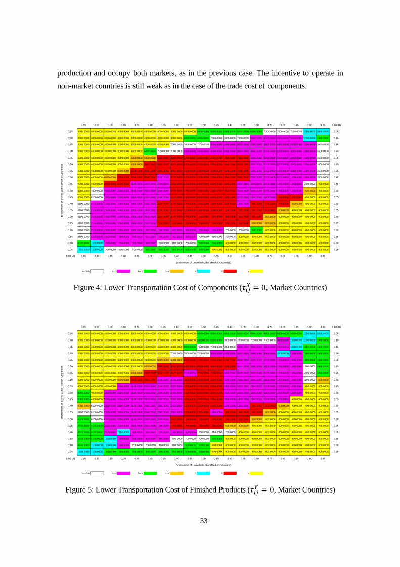
Next, let us see what happens when selected values of trade and fixed costs change.

If the transportation cost of components concerning the trade-link between the market

countries is lowered, type-H firms extend their influence (Figure 4). It is quite natural that

sending components to the foreign market country for local production becomes cheaper

than exporting finished products in this case. As the type-H firms increase, the incentive to

operate in non-market countries as a type-EV firm becomes weak.

When the transportation cost of finished products concerning the trade-link between

the market countries is lowered, type-N firms increase (Figure 5). Contrary to the previous

case, exporting finished products to the foreign market country becomes cheaper this time

than sending components for local production. Type-N firms extend their influence along

the SW-NE diagonals where the relative factor endowment and factor prices tend to be

similar in the two market countries. On the other hand, if there is a difference in factor

availability even to a slight extent, the firms established in the larger country dominate the

0.95 0.90 0.85 0.80 0.75 0.70 0.65 0.60 0.55 0.50 0.45 0.40 0.35 0.30 0.25 0.20 0.15 0.10 0.05 0.00 (D)

0.95 0.2200 0.2200 0.2200 0.2200 0.2200 0.2200 0.2200 0.2200 2200.2200 2200.2200 2200.2200 2200.2200 2200.2200 2200.2200 2200.0000 2200.0000 2200.0000 2200.0000 2200.0000 0.05

0.90 0.2200 2200.2200 2200.2200 2200.2200 2200.2200 2200.2200 2200.2200 2200.2200 2200.0000 2200.0000 2200.0000 2200.0000 2200.0000 2200.0000 2200.0000 2200.0000 2200.0000 2200.0000 2200.0000 0.10

0.85 2200.2200 2200.2200 2200.2200 2200.0000 2200.0000 2200.0000 2200.0000 2200.0000 2200.0000 2200.0000 2200.0000 2200.0000 2200.0000 2200.0000 2200.0000 2200.0000 2200.0000 2200.0000 2200.0000 0.15

0.80 2200.0000 2200.0000 2200.0000 2200.0000 2200.0000 2200.0000 2200.0000 2200.0000 2200.0000 2200.0000 2200.0000 2200.0000 2200.0000 2200.0000 2200.0000 2200.0000 2200.0000 2200.0000 2200.0000 0.20

0.75 2200.0000 2200.0000 2200.0000 2200.0000 2200.0000 2200.0000 2200.0000 2200.0000 2200.0000 2200.0000 2200.0000 2200.0000 2200.0000 2200.0000 2200.0000 2200.0000 2200.0000 2200.0000 2200.0000 0.25

0.70 2200.0000 2200.0000 2200.0000 2200.0000 2200.0000 2200.0000 2200.0000 2200.0000 2200.0000 2200.0000 2200.0000 2200.0000 2200.0000 2200.0000 2200.0000 2200.0000 2200.0000 2200.0000 2200.0000 0.30

0.65 2200.0000 2200.0000 2200.0000 2200.0000 2200.0000 2200.0000 2200.0000 2200.0000 2200.0000 2200.0000 2200.0000 2200.0000 2200.0000 2200.0000 2200.0000 2200.0000 2200.0000 2200.0000 2200.0000 0.35

0.60 2200.0000 2200.0000 2200.0000 2200.0000 2200.0000 2200.0000 2200.0000 2200.0000 2200.0000 2200.0000 2200.0000 2200.0000 2200.0000 2200.0000 2200.0000 2200.0000 2200.0000 2200.0000 2200.0000 0.40

0.55 2200.0000 2200.0000 2200.0000 2200.0000 2200.0000 2200.0000 2200.0000 2200.0000 2200.0000 2200.0000 2200.0000 2200.0000 2200.0000 2200.0000 2200.0000 2200.0000 2200.0000 2200.0000 2200.0000 0.45

0.50 2200.0000 2200.0000 2200.0000 2200.0000 2200.0000 2200.0000 2200.0000 2200.0000 2200.0000 2200.0000 2200.0000 2200.0000 2200.0000 2200.0000 2200.0000 2200.0000 2200.0000 2200.0000 2200.0000 0.50

0.45 2200.0000 2200.0000 2200.0000 2200.0000 2200.0000 2200.0000 2200.0000 2200.0000 2200.0000 2200.0000 2200.0000 2200.0000 2200.0000 2200.0000 2200.0000 2200.0000 2200.0000 2200.0000 2200.0000 0.55

0.40 2200.0000 2200.0000 2200.0000 2200.0000 2200.0000 2200.0000 2200.0000 2200.0000 2200.0000 2200.0000 2200.0000 2200.0000 2200.0000 2200.0000 2200.0000 2200.0000 2200.0000 2200.0000 2200.0000 0.60

0.35 2200.0000 2200.0000 2200.0000 2200.0000 2200.0000 2200.0000 2200.0000 2200.0000 2200.0000 2200.0000 2200.0000 2200.0000 2200.0000 2200.0000 2200.0000 2200.0000 2200.0000 2200.0000 2200.0000 0.65

0.30 2200.0000 2200.0000 2200.0000 2200.0000 2200.0000 2200.0000 2200.0000 2200.0000 2200.0000 2200.0000 2200.0000 2200.0000 2200.0000 2200.0000 2200.0000 2200.0000 2200.0000 2200.0000 2200.0000 0.70

0.25 2200.0000 2200.0000 2200.0000 2200.0000 2200.0000 2200.0000 2200.0000 2200.0000 2200.0000 2200.0000 2200.0000 2200.0000 2200.0000 2200.0000 2200.0000 2200.0000 2200.0000 2200.0000 2200.0000 0.75

0.20 2200.0000 2200.0000 2200.0000 2200.0000 2200.0000 2200.0000 2200.0000 2200.0000 2200.0000 2200.0000 2200.0000 2200.0000 2200.0000 2200.0000 2200.0000 2200.0000 2200.0000 2200.0000 2200.0000 0.80

0.15 2200.0000 2200.0000 2200.0000 2200.0000 2200.0000 2200.0000 2200.0000 2200.0000 2200.0000 2200.0000 2200.0000 2200.0000 2200.0000 2200.0000 2200.0000 2200.0000 2200.1100 2200.1100 2200.1100 0.85

0.10 2200.0000 2200.0000 2200.0000 2200.0000 2200.0000 2200.0000 2200.0000 2200.0000 2200.0000 2200.0000 2200.0000 2200.1100 2200.1100 2200.1100 2200.1100 2200.1100 2200.1100 2200.1100 0.1100 0.90

0.05 2200.0000 2200.0000 2200.0000 2200.0000 2200.0000 2200.1100 2200.1100 2200.1100 2200.1100 2200.1100 2200.1100 0.1100 0.1100 0.1100 0.1100 0.1100 0.1100 0.1100 0.1100 0.95

0.00 (C) 0.05 0.10 0.15 0.20 0.25 0.30 0.35 0.40 0.45 0.50 0.55 0.60 0.65 0.70 0.75 0.80 0.85 0.90 0.95

H+EV H EV

End

owm

ent

of S

kille

d La

bor

(Non

-Mar

ket

Cou

ntrie

s)

Endowment of Unskilled Labor (Non-Market Countries)

33

production and occupy both markets, as in the previous case. The incentive to operate in

non-market countries is still weak as in the case of the trade cost of components.

Figure 4: Lower Transportation Cost of Components ( 0, Market Countries)

Figure 5: Lower Transportation Cost of Finished Products ( 0, Market Countries)

0.95 0.90 0.85 0.80 0.75 0.70 0.65 0.60 0.55 0.50 0.45 0.40 0.35 0.30 0.25 0.20 0.15 0.10 0.05 0.00 (B)

0.95 4000.0000 4000.0000 4000.0000 4000.0000 4000.0000 4000.0000 4000.0000 4000.0000 4000.0000 5000.0000 5000.0000 5000.0000 5000.0000 5000.0000 7000.0000 7000.0000 7000.0000 1000.0000 1000.0000 0.05

0.90 4000.0000 4000.0000 4000.0000 4000.0000 4000.0000 4000.0000 4000.0000 4000.0000 5000.0000 5000.0000 7000.0000 7000.0000 7000.0000 3000.0000 3000.0000 3000.0000 3000.0000 1000.0000 1400.0000 0.10

0.85 4000.0000 4000.0000 4000.0000 4000.0000 4000.0000 4000.0000 4000.0000 7000.0000 7000.0000 7000.0000 3000.0000 3000.0000 3000.0000 3000.0000 3000.0000 3000.0000 3200.0000 1200.0000 1600.0000 0.15

0.80 4000.0000 4000.0000 4000.0000 4000.0000 4000.0000 5000.0000 7000.0000 7000.0000 3000.0000 3000.0000 3000.0000 3000.0000 3000.0000 3000.0000 3200.0000 3200.0000 3200.0000 1200.0000 1600.0000 0.20

0.75 4000.0000 4000.0000 4000.0000 4000.0000 6000.0000 6000.0000 2000.0000 2000.0000 2000.0000 2000.0000 2000.0000 2000.0000 2000.0000 3200.0000 3200.0000 3200.0000 3200.0000 1200.0000 1600.0000 0.25

0.70 4000.0000 4000.0000 4000.0000 4000.0000 6000.0000 2000.0000 2000.0000 2000.0000 2000.0000 2000.0000 2200.0000 2200.0000 2200.0000 3200.0000 3200.0000 3200.0000 3200.0000 1200.0000 1600.0000 0.30

0.65 4000.0000 4000.0000 4000.0000 6000.0000 2000.0000 2000.0000 2000.0000 2000.0000 2200.0000 2200.0000 2200.0000 2200.0000 2200.0000 3200.0000 3200.0000 3200.0000 3200.0000 1200.0000 1600.0000 0.35

0.60 4000.0000 4000.0000 6000.0000 2000.0000 2000.0000 2000.0000 2100.0000 2200.0000 2200.0000 2200.0000 2200.0000 2200.0000 2200.0000 3200.0000 3200.0000 3200.0000 1200.0000 1200.0000 1600.0000 0.40

0.55 4000.0000 4000.0000 2000.0000 2000.0000 2100.0000 2100.0000 2300.0000 2200.0000 2200.0000 2200.0000 2200.0000 2200.0000 3200.0000 3200.0000 3200.0000 1200.0000 1200.0000 1600.0000 400.0000 0.45

0.50 4000.0000 7000.0000 2100.0000 2100.0000 2100.0000 2300.0000 2300.0000 2200.0000 2200.0000 2200.0000 2200.0000 2200.0000 3200.0000 3200.0000 1200.0000 1200.0000 1200.0000 600.0000 400.0000 0.50

0.45 4000.0000 6100.0000 2100.0000 2100.0000 2300.0000 2300.0000 2300.0000 2200.0000 2200.0000 2200.0000 2200.0000 2200.0000 3200.0000 1200.0000 1200.0000 200.0000 200.0000 400.0000 400.0000 0.55

0.40 6100.0000 2100.0000 2100.0000 2300.0000 2300.0000 2300.0000 2200.0000 2200.0000 2200.0000 2200.0000 2200.0000 2200.0000 1200.0000 200.0000 200.0000 200.0000 600.0000 400.0000 400.0000 0.60

0.35 6100.0000 2100.0000 2300.0000 2300.0000 2300.0000 2300.0000 2200.0000 2200.0000 2200.0000 2200.0000 2200.0000 200.0000 200.0000 200.0000 200.0000 600.0000 400.0000 400.0000 400.0000 0.65

0.30 6100.0000 2100.0000 2300.0000 2300.0000 2300.0000 2300.0000 2200.0000 2200.0000 2200.0000 200.0000 200.0000 200.0000 200.0000 200.0000 600.0000 400.0000 400.0000 400.0000 400.0000 0.70

0.25 6100.0000 2100.0000 2300.0000 2300.0000 2300.0000 2300.0000 200.0000 200.0000 200.0000 200.0000 200.0000 200.0000 200.0000 600.0000 600.0000 400.0000 400.0000 400.0000 400.0000 0.75

0.20 6100.0000 2100.0000 2300.0000 2300.0000 2300.0000 300.0000 300.0000 300.0000 300.0000 300.0000 300.0000 700.0000 700.0000 500.0000 400.0000 400.0000 400.0000 400.0000 400.0000 0.80

0.15 6100.0000 2100.0000 2300.0000 300.0000 300.0000 300.0000 300.0000 300.0000 300.0000 700.0000 700.0000 700.0000 400.0000 400.0000 400.0000 400.0000 400.0000 400.0000 400.0000 0.85

0.10 4100.0000 100.0000 300.0000 300.0000 300.0000 300.0000 700.0000 700.0000 700.0000 500.0000 500.0000 400.0000 400.0000 400.0000 400.0000 400.0000 400.0000 400.0000 400.0000 0.90

0.05 100.0000 100.0000 700.0000 700.0000 700.0000 500.0000 500.0000 500.0000 500.0000 500.0000 400.0000 400.0000 400.0000 400.0000 400.0000 400.0000 400.0000 400.0000 400.0000 0.95

0.00 (A) 0.05 0.10 0.15 0.20 0.25 0.30 0.35 0.40 0.45 0.50 0.55 0.60 0.65 0.70 0.75 0.80 0.85 0.90 0.95

N+H+V N+H N+V H+V N H V

End

owm

ent

of S

kille

d La

bor

(Mar

ket

Cou

ntrie

s)

Endowment of Unskilled Labor (Market Countries)

0.95 0.90 0.85 0.80 0.75 0.70 0.65 0.60 0.55 0.50 0.45 0.40 0.35 0.30 0.25 0.20 0.15 0.10 0.05 0.00 (B)

0.95 4000.0000 4000.0000 4000.0000 4000.0000 4000.0000 4000.0000 4000.0000 4000.0000 4000.0000 5000.0000 5000.0000 5000.0000 5000.0000 5000.0000 5000.0000 5000.0000 5000.0000 1000.0000 1000.0000 0.05

0.90 4000.0000 4000.0000 4000.0000 4000.0000 4000.0000 4000.0000 4000.0000 4000.0000 4000.0000 5000.0000 5000.0000 7000.0000 7000.0000 7000.0000 7000.0000 3000.0000 1000.0000 1000.0000 1400.0000 0.10

0.85 4000.0000 4000.0000 4000.0000 4000.0000 4000.0000 4000.0000 4000.0000 4000.0000 5000.0000 7000.0000 7000.0000 7000.0000 3000.0000 3000.0000 3000.0000 3000.0000 1000.0000 1400.0000 1400.0000 0.15

0.80 4000.0000 4000.0000 4000.0000 4000.0000 4000.0000 4000.0000 4000.0000 7000.0000 7000.0000 7000.0000 3000.0000 3000.0000 3000.0000 3000.0000 3000.0000 1000.0000 1200.0000 1400.0000 1400.0000 0.20

0.75 4000.0000 4000.0000 4000.0000 4000.0000 4000.0000 4000.0000 6000.0000 6000.0000 2000.0000 2000.0000 2000.0000 2000.0000 3000.0000 3200.0000 3200.0000 1200.0000 1200.0000 1400.0000 1400.0000 0.25

0.70 4000.0000 4000.0000 4000.0000 4000.0000 4000.0000 6000.0000 2000.0000 2000.0000 2000.0000 2000.0000 2000.0000 2200.0000 3200.0000 3200.0000 1200.0000 1200.0000 1200.0000 1600.0000 1400.0000 0.30

0.65 4000.0000 4000.0000 4000.0000 4000.0000 6000.0000 2000.0000 2000.0000 2000.0000 2100.0000 2200.0000 2200.0000 3200.0000 3200.0000 3200.0000 1200.0000 1200.0000 1200.0000 1600.0000 1400.0000 0.35

0.60 4000.0000 4000.0000 4000.0000 6000.0000 2000.0000 2000.0000 2100.0000 2100.0000 2200.0000 2200.0000 2200.0000 3200.0000 3200.0000 3200.0000 1200.0000 1200.0000 1200.0000 1600.0000 600.0000 0.40

0.55 4000.0000 4000.0000 4000.0000 2100.0000 2100.0000 2100.0000 2100.0000 2300.0000 2200.0000 2200.0000 2200.0000 3200.0000 3200.0000 1200.0000 1200.0000 1200.0000 1200.0000 400.0000 400.0000 0.45

0.50 5000.0000 4000.0000 2100.0000 2100.0000 2100.0000 2100.0000 2300.0000 2300.0000 2200.0000 2200.0000 2200.0000 3200.0000 3200.0000 1200.0000 1200.0000 1200.0000 1200.0000 400.0000 400.0000 0.50

0.45 5000.0000 4000.0000 2100.0000 2100.0000 2100.0000 2100.0000 2300.0000 2300.0000 2200.0000 2200.0000 2200.0000 3200.0000 1200.0000 1200.0000 1200.0000 1200.0000 400.0000 400.0000 400.0000 0.55

0.40 6000.0000 6100.0000 2100.0000 2100.0000 2100.0000 2300.0000 2300.0000 2300.0000 2200.0000 2200.0000 2200.0000 1200.0000 1200.0000 200.0000 200.0000 600.0000 400.0000 400.0000 400.0000 0.60

0.35 6100.0000 6100.0000 2100.0000 2100.0000 2100.0000 2300.0000 2300.0000 2300.0000 2200.0000 2200.0000 1200.0000 200.0000 200.0000 200.0000 600.0000 400.0000 400.0000 400.0000 400.0000 0.65

0.30 4100.0000 6100.0000 2100.0000 2100.0000 2100.0000 2300.0000 2300.0000 2200.0000 200.0000 200.0000 200.0000 200.0000 200.0000 600.0000 400.0000 400.0000 400.0000 400.0000 400.0000 0.70

0.25 4100.0000 4100.0000 2100.0000 2100.0000 2300.0000 2300.0000 300.0000 200.0000 200.0000 200.0000 200.0000 600.0000 600.0000 400.0000 400.0000 400.0000 400.0000 400.0000 400.0000 0.75

0.20 4100.0000 4100.0000 2100.0000 100.0000 300.0000 300.0000 300.0000 300.0000 300.0000 700.0000 700.0000 700.0000 400.0000 400.0000 400.0000 400.0000 400.0000 400.0000 400.0000 0.80

0.15 4100.0000 4100.0000 100.0000 300.0000 300.0000 300.0000 300.0000 700.0000 700.0000 700.0000 500.0000 400.0000 400.0000 400.0000 400.0000 400.0000 400.0000 400.0000 400.0000 0.85

0.10 4100.0000 100.0000 100.0000 300.0000 700.0000 700.0000 700.0000 700.0000 500.0000 500.0000 400.0000 400.0000 400.0000 400.0000 400.0000 400.0000 400.0000 400.0000 400.0000 0.90

0.05 100.0000 100.0000 500.0000 500.0000 500.0000 500.0000 500.0000 500.0000 500.0000 500.0000 400.0000 400.0000 400.0000 400.0000 400.0000 400.0000 400.0000 400.0000 400.0000 0.95

0.00 (A) 0.05 0.10 0.15 0.20 0.25 0.30 0.35 0.40 0.45 0.50 0.55 0.60 0.65 0.70 0.75 0.80 0.85 0.90 0.95

N+H+V N+H N+V H+V N H V

End

owm

ent

of S

kille

d La

bor

(Mar

ket

Cou

ntrie

s)

Endowment of Unskilled Labor (Market Countries)

34

Figure 6: Lower Import Tariff on Components ( 0, Market Countries)

Figure 7: Lower Import Tariff on Finished Products ( 0, Market Countries)

Let us move to the case of import tariff. The main difference between transportation

cost and import tariff is that a decrease in the former tends to reduce demand for the

0.95 0.90 0.85 0.80 0.75 0.70 0.65 0.60 0.55 0.50 0.45 0.40 0.35 0.30 0.25 0.20 0.15 0.10 0.05 0.00 (B)

0.95 4000.0000 4000.0000 4000.0000 4000.0000 4000.0000 4000.0000 4000.0000 4000.0000 4000.0000 5000.0000 5000.0000 5000.0000 5000.0000 5000.0000 7000.0000 7000.0000 7000.0000 3000.0000 1000.0000 0.05

0.90 4000.0000 4000.0000 4000.0000 4000.0000 4000.0000 4000.0000 4000.0000 4000.0000 5000.0000 5000.0000 7000.0000 7000.0000 7000.0000 3000.0000 3000.0000 3000.0000 3000.0000 1200.0000 1400.0000 0.10

0.85 4000.0000 4000.0000 4000.0000 4000.0000 4000.0000 4000.0000 4000.0000 7000.0000 7000.0000 7000.0000 7000.0000 3000.0000 3000.0000 3000.0000 3000.0000 3000.0000 3200.0000 1200.0000 1600.0000 0.15

0.80 4000.0000 4000.0000 4000.0000 4000.0000 4000.0000 5000.0000 7000.0000 7000.0000 3000.0000 3000.0000 3000.0000 3000.0000 3000.0000 3000.0000 3200.0000 3200.0000 3200.0000 1200.0000 3300.0000 0.20

0.75 4000.0000 4000.0000 4000.0000 4000.0000 6000.0000 6000.0000 2000.0000 2000.0000 2000.0000 2000.0000 2000.0000 2000.0000 2200.0000 3200.0000 3200.0000 3200.0000 3200.0000 1200.0000 1300.0000 0.25

0.70 4000.0000 4000.0000 4000.0000 4000.0000 6000.0000 2000.0000 2000.0000 2000.0000 2000.0000 2000.0000 2200.0000 2200.0000 2200.0000 3200.0000 3200.0000 3200.0000 3200.0000 1200.0000 1600.0000 0.30

0.65 4000.0000 4000.0000 4000.0000 6000.0000 2000.0000 2000.0000 2000.0000 2000.0000 2200.0000 2200.0000 2200.0000 2200.0000 2200.0000 3200.0000 3200.0000 3200.0000 3200.0000 1200.0000 1600.0000 0.35

0.60 4000.0000 4000.0000 6000.0000 2000.0000 2000.0000 2000.0000 2200.0000 2200.0000 2200.0000 2200.0000 2200.0000 2200.0000 2200.0000 3200.0000 3200.0000 3200.0000 1200.0000 1200.0000 600.0000 0.40

0.55 5000.0000 5000.0000 2000.0000 2000.0000 2100.0000 2300.0000 2200.0000 2200.0000 2200.0000 2200.0000 2200.0000 2200.0000 2200.0000 3200.0000 3200.0000 3200.0000 1200.0000 1600.0000 400.0000 0.45

0.50 5000.0000 7000.0000 2100.0000 2100.0000 2300.0000 2300.0000 2200.0000 2200.0000 2200.0000 2200.0000 2200.0000 2200.0000 2200.0000 3200.0000 3200.0000 1200.0000 1200.0000 700.0000 500.0000 0.50

0.45 4000.0000 6100.0000 2100.0000 2300.0000 2300.0000 2300.0000 2200.0000 2200.0000 2200.0000 2200.0000 2200.0000 2200.0000 2200.0000 3200.0000 1200.0000 200.0000 200.0000 500.0000 500.0000 0.55

0.40 6000.0000 2100.0000 2100.0000 2300.0000 2300.0000 2300.0000 2200.0000 2200.0000 2200.0000 2200.0000 2200.0000 2200.0000 2200.0000 200.0000 200.0000 200.0000 600.0000 400.0000 400.0000 0.60

0.35 6100.0000 2100.0000 2300.0000 2300.0000 2300.0000 2300.0000 2200.0000 2200.0000 2200.0000 2200.0000 2200.0000 200.0000 200.0000 200.0000 200.0000 600.0000 400.0000 400.0000 400.0000 0.65

0.30 6100.0000 2100.0000 2300.0000 2300.0000 2300.0000 2300.0000 2200.0000 2200.0000 2200.0000 200.0000 200.0000 200.0000 200.0000 200.0000 600.0000 400.0000 400.0000 400.0000 400.0000 0.70

0.25 3100.0000 2100.0000 2300.0000 2300.0000 2300.0000 2300.0000 2200.0000 200.0000 200.0000 200.0000 200.0000 200.0000 200.0000 600.0000 600.0000 400.0000 400.0000 400.0000 400.0000 0.75

0.20 3300.0000 2100.0000 2300.0000 2300.0000 2300.0000 300.0000 300.0000 300.0000 300.0000 300.0000 300.0000 700.0000 700.0000 500.0000 400.0000 400.0000 400.0000 400.0000 400.0000 0.80

0.15 6100.0000 2100.0000 2300.0000 300.0000 300.0000 300.0000 300.0000 300.0000 700.0000 700.0000 700.0000 700.0000 400.0000 400.0000 400.0000 400.0000 400.0000 400.0000 400.0000 0.85

0.10 4100.0000 2100.0000 300.0000 300.0000 300.0000 300.0000 700.0000 700.0000 700.0000 500.0000 500.0000 400.0000 400.0000 400.0000 400.0000 400.0000 400.0000 400.0000 400.0000 0.90

0.05 100.0000 300.0000 700.0000 700.0000 700.0000 500.0000 500.0000 500.0000 500.0000 500.0000 400.0000 400.0000 400.0000 400.0000 400.0000 400.0000 400.0000 400.0000 400.0000 0.95

0.00 (A) 0.05 0.10 0.15 0.20 0.25 0.30 0.35 0.40 0.45 0.50 0.55 0.60 0.65 0.70 0.75 0.80 0.85 0.90 0.95

N+H+V N+H N+V H+V N H V

End

owm

ent

of S

kille

d La

bor

(Mar

ket

Cou

ntrie

s)

Endowment of Unskilled Labor (Market Countries)

0.95 0.90 0.85 0.80 0.75 0.70 0.65 0.60 0.55 0.50 0.45 0.40 0.35 0.30 0.25 0.20 0.15 0.10 0.05 0.00 (B)

0.95 5000.0000 4000.0000 4000.0000 4000.0000 4000.0000 4000.0000 4000.0000 4000.0000 4000.0000 5000.0000 5000.0000 5000.0000 5000.0000 5000.0000 5000.0000 5000.0000 5000.0000 1000.0000 1000.0000 0.05

0.90 4000.0000 4000.0000 4000.0000 4000.0000 4000.0000 4000.0000 4000.0000 4000.0000 4000.0000 4000.0000 5000.0000 5000.0000 5000.0000 5000.0000 5000.0000 5000.0000 1000.0000 1000.0000 1400.0000 0.10

0.85 4000.0000 4000.0000 5000.0000 4000.0000 4000.0000 4000.0000 4000.0000 4000.0000 5000.0000 7000.0000 7000.0000 7000.0000 7000.0000 5000.0000 5000.0000 1000.0000 1000.0000 1400.0000 1400.0000 0.15

0.80 4000.0000 5000.0000 4000.0000 4000.0000 4000.0000 4000.0000 4000.0000 6000.0000 6000.0000 7000.0000 7000.0000 7000.0000 7000.0000 3000.0000 1000.0000 1000.0000 1400.0000 1400.0000 1400.0000 0.20

0.75 5000.0000 5000.0000 4000.0000 4000.0000 4000.0000 4000.0000 4000.0000 6000.0000 6000.0000 6000.0000 3000.0000 3000.0000 3000.0000 1000.0000 1000.0000 1400.0000 1400.0000 1400.0000 1400.0000 0.25

0.70 4000.0000 4000.0000 4000.0000 4000.0000 4000.0000 4000.0000 6000.0000 6000.0000 2000.0000 3000.0000 3000.0000 3000.0000 1000.0000 1000.0000 1400.0000 1400.0000 1400.0000 1400.0000 1400.0000 0.30

0.65 4000.0000 5000.0000 4000.0000 4000.0000 4000.0000 4100.0000 6000.0000 2100.0000 2100.0000 3100.0000 3100.0000 3100.0000 1000.0000 1400.0000 1400.0000 1400.0000 1400.0000 1400.0000 1400.0000 0.35

0.60 4000.0000 4000.0000 4000.0000 4000.0000 4100.0000 4100.0000 2100.0000 2100.0000 3100.0000 3100.0000 3100.0000 1000.0000 1200.0000 1400.0000 1400.0000 1400.0000 1400.0000 1400.0000 500.0000 0.40

0.55 5000.0000 4000.0000 4000.0000 4100.0000 4100.0000 4100.0000 2100.0000 2100.0000 3100.0000 3100.0000 1100.0000 1200.0000 1200.0000 1400.0000 1400.0000 1400.0000 1400.0000 400.0000 500.0000 0.45

0.50 5000.0000 4000.0000 4100.0000 4100.0000 4100.0000 4100.0000 2100.0000 2100.0000 3100.0000 1100.0000 1300.0000 1200.0000 1200.0000 1400.0000 1400.0000 1400.0000 1400.0000 400.0000 500.0000 0.50

0.45 5000.0000 4000.0000 4100.0000 4100.0000 4100.0000 4100.0000 2100.0000 2100.0000 1100.0000 1300.0000 1300.0000 1200.0000 1200.0000 1400.0000 1400.0000 1400.0000 400.0000 400.0000 500.0000 0.55

0.40 5000.0000 4100.0000 4100.0000 4100.0000 4100.0000 4100.0000 2100.0000 100.0000 1300.0000 1300.0000 1300.0000 1200.0000 1200.0000 1400.0000 1400.0000 400.0000 400.0000 400.0000 400.0000 0.60

0.35 5000.0000 4100.0000 4100.0000 4100.0000 4100.0000 4100.0000 100.0000 1300.0000 1300.0000 1300.0000 1200.0000 1200.0000 600.0000 1400.0000 400.0000 400.0000 400.0000 500.0000 400.0000 0.65

0.30 4100.0000 4100.0000 4100.0000 4100.0000 4100.0000 100.0000 100.0000 300.0000 300.0000 300.0000 200.0000 600.0000 600.0000 400.0000 400.0000 400.0000 400.0000 400.0000 400.0000 0.70

0.25 4100.0000 4100.0000 4100.0000 4100.0000 100.0000 100.0000 300.0000 300.0000 300.0000 600.0000 600.0000 600.0000 400.0000 400.0000 400.0000 400.0000 400.0000 500.0000 500.0000 0.75

0.20 4100.0000 4100.0000 4100.0000 100.0000 100.0000 300.0000 700.0000 700.0000 700.0000 700.0000 600.0000 600.0000 400.0000 400.0000 400.0000 400.0000 400.0000 500.0000 500.0000 0.80

0.15 4100.0000 4100.0000 100.0000 100.0000 500.0000 500.0000 700.0000 700.0000 700.0000 700.0000 500.0000 400.0000 400.0000 400.0000 400.0000 400.0000 500.0000 400.0000 500.0000 0.85

0.10 4100.0000 100.0000 100.0000 500.0000 500.0000 500.0000 500.0000 500.0000 500.0000 400.0000 400.0000 400.0000 400.0000 400.0000 400.0000 400.0000 400.0000 400.0000 400.0000 0.90

0.05 100.0000 100.0000 500.0000 500.0000 500.0000 500.0000 500.0000 500.0000 500.0000 500.0000 400.0000 400.0000 400.0000 400.0000 400.0000 400.0000 400.0000 400.0000 500.0000 0.95

0.00 (A) 0.05 0.10 0.15 0.20 0.25 0.30 0.35 0.40 0.45 0.50 0.55 0.60 0.65 0.70 0.75 0.80 0.85 0.90 0.95

N+H+V N+H N+V H+V N H V

End

owm

ent

of S

kille

d La

bor

(Mar

ket

Cou

ntrie

s)

Endowment of Unskilled Labor (Market Countries)

35

unskilled labor in the exporting country so that the relative wage of the factor depreciates,

while a decrease in the latter just reduces income in the importing country. If the import

tariff on components concerning the trade-link between two market countries is lowered,

type-H firms extend their influence as in the case of transportation cost (Figure 6). In the

present setting, the difference between transportation cost and import tariff noted above

does not crucially affect the simulation results so that directions of the effects of lowering

two items are identical. On the other hand, the volume of the effects is larger in this case of

import tariff because the initial rate is much higher (0.2) than the one of transportation cost

(0.1). This tendency is quite obvious if we see the case when the import tariff on finished

products concerning the trade-link between the market countries is lowered. Figure 7 shows

that type-H firms are replaced by type-N and type-V especially around the four corners.

Figure 8: Lower Transportation Cost of Finished Products

( 0, Non-Market Countries)

When two non-market countries differ in size and relative factor endowment,

lowering the transportation cost of finished products concerning the trade-link just between

countries and motivates firms established in country to be type-EH and operate

in country . This phenomenon is obvious around the SE part in Figure 8, where the price

of unskilled labor in country is relatively cheap. This result is consistent with the one

0.95 0.90 0.85 0.80 0.75 0.70 0.65 0.60 0.55 0.50 0.45 0.40 0.35 0.30 0.25 0.20 0.15 0.10 0.05 0.00 (D)

0.95 0.2200 0.2200 0.2200 0.2200 0.2200 0.2200 0.2200 0.2200 2200.2200 2200.2200 2200.2200 2200.2200 2200.2200 2200.2200 2200.0000 2200.0000 2200.0000 2200.0000 2200.0000 0.05

0.90 0.2200 2200.2200 2200.2200 2200.2200 2200.2200 2200.2200 2200.2200 2200.2200 2200.0000 2200.0000 2200.0000 2200.0000 2200.0000 2200.0000 2200.0000 2200.0000 2200.0000 2200.0000 2200.0000 0.10

0.85 2200.2200 2200.2200 2200.2200 2200.0000 2200.0000 2200.0000 2200.0000 2200.0000 2200.0000 2200.0000 2200.0000 2200.0000 2200.0000 2200.0000 2200.0000 2200.0000 2200.0000 2200.0000 2200.0000 0.15

0.80 2200.0000 2200.0000 2200.0000 2200.0000 2200.0000 2200.0000 2200.0000 2200.0000 2200.0000 2200.0000 2200.0000 2200.0000 2200.0000 2200.0000 2200.0000 2200.0000 2200.0000 2200.0000 2200.0000 0.20

0.75 2200.0000 2200.0000 2200.0000 2200.0000 2200.0000 2200.0000 2200.0000 2200.0000 2200.0000 2200.0000 2200.0000 2200.0000 2200.0000 2200.0000 2200.0000 2200.0000 2200.0000 2200.0000 2200.0000 0.25

0.70 2200.0000 2200.0000 2200.0000 2200.0000 2200.0000 2200.0000 2200.0000 2200.0000 2200.0000 2200.0000 2200.0000 2200.0000 2200.0000 2200.0000 2200.0000 2200.0000 2200.0000 2200.0000 2200.0000 0.30

0.65 2200.0000 2200.0000 2200.0000 2200.0000 2200.0000 2200.0000 2200.0000 2200.0000 2200.0000 2200.0000 2200.0000 2200.0000 2200.0000 2200.0000 2200.0000 2200.0000 2200.0000 2200.0000 2200.0000 0.35

0.60 2200.0000 2200.0000 2200.0000 2200.0000 2200.0000 2200.0000 2200.0000 2200.0000 2200.0000 2200.0000 2200.0000 2200.0000 2200.0000 2200.0000 2200.0000 2200.0000 2200.0000 2200.0000 2200.0000 0.40

0.55 2200.0000 2200.0000 2200.0000 2200.0000 2200.0000 2200.0000 2200.0000 2200.0000 2200.0000 2200.0000 2200.0000 2200.0000 2200.0000 2200.0000 2200.0000 2200.0000 2200.0000 2200.0000 2200.0000 0.45

0.50 2200.0000 2200.0000 2200.0000 2200.0000 2200.0000 2200.0000 2200.0000 2200.0000 2200.0000 2200.0000 2200.0000 2200.0000 2200.0000 2200.0000 2200.0000 2200.0000 2200.0000 2200.0000 2200.0000 0.50

0.45 2200.0000 2200.0000 2200.0000 2200.0000 2200.0000 2200.0000 2200.0000 2200.0000 2200.0000 2200.0000 2200.0000 2200.0000 2200.0000 2200.0000 2200.0000 2200.0000 2200.0000 2200.0000 2200.0000 0.55

0.40 2200.0000 2200.0000 2200.0000 2200.0000 2200.0000 2200.0000 2200.0000 2200.0000 2200.0000 2200.0000 2200.0000 2200.0000 2200.0000 2200.0000 2200.0000 2200.0000 2200.0000 2200.0000 2200.0000 0.60

0.35 2200.0000 2200.0000 2200.0000 2200.0000 2200.0000 2200.0000 2200.0000 2200.0000 2200.0000 2200.0000 2200.0000 2200.0000 2200.0000 2200.0000 2200.0000 2200.0000 2200.0000 2200.0000 2200.0000 0.65

0.30 2200.0000 2200.0000 2200.0000 2200.0000 2200.0000 2200.0000 2200.0000 2200.0000 2200.0000 2200.0000 2200.0000 2200.0000 2200.0000 2200.0000 2200.0000 2200.0000 2200.0000 2200.0000 2200.0000 0.70

0.25 2200.0000 2200.0000 2200.0000 2200.0000 2200.0000 2200.0000 2200.0000 2200.0000 2200.0000 2200.0000 2200.0000 2200.0000 2200.0000 2200.0000 2200.0000 2200.0000 2200.0000 2200.0000 2200.0000 0.75

0.20 2200.0000 2200.0000 2200.0000 2200.0000 2200.0000 2200.0000 2200.0000 2200.0000 2200.0000 2200.0000 2200.0000 2200.0000 2200.0000 2200.0000 2200.0000 2201.0000 2201.0000 2201.1000 2201.1000 0.80

0.15 2200.0000 2200.0000 2200.0000 2200.0000 2200.0000 2200.0000 2200.0000 2200.0000 2200.0000 2200.0000 2200.0000 2201.0000 2201.1000 2201.1000 2201.1000 2200.1000 200.1000 200.1100 200.1100 0.85

0.10 2200.0000 2200.0000 2200.0000 2200.0000 2200.0000 2200.0000 2200.0000 2201.0000 2201.1000 2201.1000 2200.1000 200.1100 200.1100 200.1100 300.1100 100.1100 0.1100 0.1100 0.1100 0.90

0.05 2200.0000 2200.0000 2200.0000 2201.0000 2201.1000 2200.1000 200.1100 300.1100 300.1100 300.1100 0.1100 0.1100 0.1100 0.1100 0.1100 0.1100 0.1100 0.1100 0.1100 0.95

0.00 (C) 0.05 0.10 0.15 0.20 0.25 0.30 0.35 0.40 0.45 0.50 0.55 0.60 0.65 0.70 0.75 0.80 0.85 0.90 0.95

N+H+EV H+EH+EV N+EV H+EH H+EV H EV

End

owm

ent

of S

kille

d La

bor

(Non

-Mar

ket

Cou

ntrie

s)

Endowment of Unskilled Labor (Non-Market Countries)

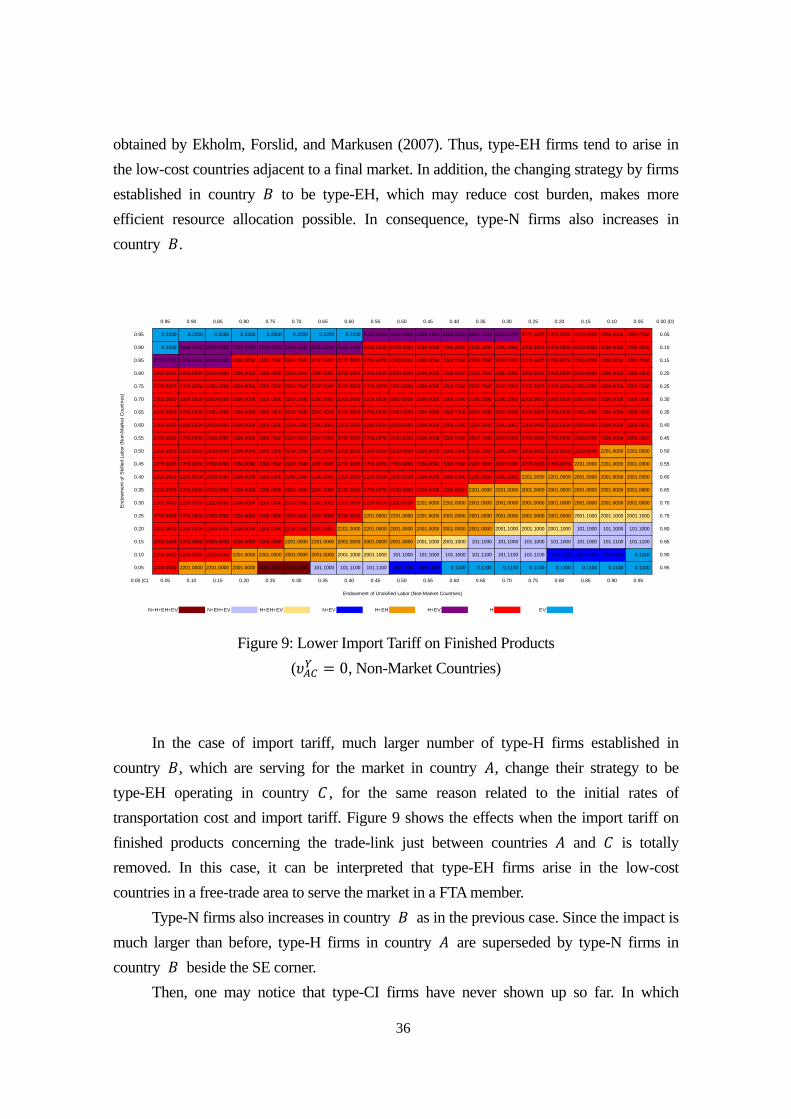
36

obtained by Ekholm, Forslid, and Markusen (2007). Thus, type-EH firms tend to arise in

the low-cost countries adjacent to a final market. In addition, the changing strategy by firms

established in country to be type-EH, which may reduce cost burden, makes more

efficient resource allocation possible. In consequence, type-N firms also increases in

country .

Figure 9: Lower Import Tariff on Finished Products

( 0, Non-Market Countries)

In the case of import tariff, much larger number of type-H firms established in

country , which are serving for the market in country , change their strategy to be

type-EH operating in country , for the same reason related to the initial rates of

transportation cost and import tariff. Figure 9 shows the effects when the import tariff on

finished products concerning the trade-link just between countries and is totally

removed. In this case, it can be interpreted that type-EH firms arise in the low-cost

countries in a free-trade area to serve the market in a FTA member.

Type-N firms also increases in country as in the previous case. Since the impact is

much larger than before, type-H firms in country are superseded by type-N firms in

country beside the SE corner.

Then, one may notice that type-CI firms have never shown up so far. In which

0.95 0.90 0.85 0.80 0.75 0.70 0.65 0.60 0.55 0.50 0.45 0.40 0.35 0.30 0.25 0.20 0.15 0.10 0.05 0.00 (D)

0.95 0.2200 0.2200 0.2200 0.2200 0.2200 0.2200 0.2200 0.2200 2200.2200 2200.2200 2200.2200 2200.2200 2200.2200 2200.2200 2200.0000 2200.0000 2200.0000 2200.0000 2200.0000 0.05

0.90 0.2200 2200.2200 2200.2200 2200.2200 2200.2200 2200.2200 2200.2200 2200.2200 2200.0000 2200.0000 2200.0000 2200.0000 2200.0000 2200.0000 2200.0000 2200.0000 2200.0000 2200.0000 2200.0000 0.10

0.85 2200.2200 2200.2200 2200.2200 2200.0000 2200.0000 2200.0000 2200.0000 2200.0000 2200.0000 2200.0000 2200.0000 2200.0000 2200.0000 2200.0000 2200.0000 2200.0000 2200.0000 2200.0000 2200.0000 0.15

0.80 2200.0000 2200.0000 2200.0000 2200.0000 2200.0000 2200.0000 2200.0000 2200.0000 2200.0000 2200.0000 2200.0000 2200.0000 2200.0000 2200.0000 2200.0000 2200.0000 2200.0000 2200.0000 2200.0000 0.20

0.75 2200.0000 2200.0000 2200.0000 2200.0000 2200.0000 2200.0000 2200.0000 2200.0000 2200.0000 2200.0000 2200.0000 2200.0000 2200.0000 2200.0000 2200.0000 2200.0000 2200.0000 2200.0000 2200.0000 0.25

0.70 2200.0000 2200.0000 2200.0000 2200.0000 2200.0000 2200.0000 2200.0000 2200.0000 2200.0000 2200.0000 2200.0000 2200.0000 2200.0000 2200.0000 2200.0000 2200.0000 2200.0000 2200.0000 2200.0000 0.30

0.65 2200.0000 2200.0000 2200.0000 2200.0000 2200.0000 2200.0000 2200.0000 2200.0000 2200.0000 2200.0000 2200.0000 2200.0000 2200.0000 2200.0000 2200.0000 2200.0000 2200.0000 2200.0000 2200.0000 0.35

0.60 2200.0000 2200.0000 2200.0000 2200.0000 2200.0000 2200.0000 2200.0000 2200.0000 2200.0000 2200.0000 2200.0000 2200.0000 2200.0000 2200.0000 2200.0000 2200.0000 2200.0000 2200.0000 2200.0000 0.40

0.55 2200.0000 2200.0000 2200.0000 2200.0000 2200.0000 2200.0000 2200.0000 2200.0000 2200.0000 2200.0000 2200.0000 2200.0000 2200.0000 2200.0000 2200.0000 2200.0000 2200.0000 2200.0000 2200.0000 0.45

0.50 2200.0000 2200.0000 2200.0000 2200.0000 2200.0000 2200.0000 2200.0000 2200.0000 2200.0000 2200.0000 2200.0000 2200.0000 2200.0000 2200.0000 2200.0000 2200.0000 2200.0000 2201.0000 2201.0000 0.50

0.45 2200.0000 2200.0000 2200.0000 2200.0000 2200.0000 2200.0000 2200.0000 2200.0000 2200.0000 2200.0000 2200.0000 2200.0000 2200.0000 2200.0000 2200.0000 2200.0000 2201.0000 2201.0000 2001.0000 0.55

0.40 2200.0000 2200.0000 2200.0000 2200.0000 2200.0000 2200.0000 2200.0000 2200.0000 2200.0000 2200.0000 2200.0000 2200.0000 2200.0000 2200.0000 2201.0000 2201.0000 2001.0000 2001.0000 2001.0000 0.60

0.35 2200.0000 2200.0000 2200.0000 2200.0000 2200.0000 2200.0000 2200.0000 2200.0000 2200.0000 2200.0000 2200.0000 2200.0000 2201.0000 2201.0000 2001.0000 2001.0000 2001.0000 2001.0000 2001.0000 0.65

0.30 2200.0000 2200.0000 2200.0000 2200.0000 2200.0000 2200.0000 2200.0000 2200.0000 2200.0000 2200.0000 2201.0000 2201.0000 2001.0000 2001.0000 2001.0000 2001.0000 2001.0000 2001.0000 2001.0000 0.70

0.25 2200.0000 2200.0000 2200.0000 2200.0000 2200.0000 2200.0000 2200.0000 2200.0000 2201.0000 2201.0000 2201.0000 2001.0000 2001.0000 2001.0000 2001.0000 2001.0000 2001.1000 2001.1000 2001.1000 0.75

0.20 2200.0000 2200.0000 2200.0000 2200.0000 2200.0000 2200.0000 2200.0000 2201.0000 2201.0000 2001.0000 2001.0000 2001.0000 2001.0000 2001.1000 2001.1000 2001.1000 101.1000 101.1000 101.1000 0.80

0.15 2200.0000 2200.0000 2200.0000 2200.0000 2200.0000 2201.0000 2201.0000 2001.0000 2001.0000 2001.0000 2001.1000 2001.1000 101.1000 101.1000 101.1000 101.1000 101.1000 101.1100 101.1100 0.85

0.10 2200.0000 2200.0000 2200.0000 2201.0000 2201.0000 2001.0000 2001.0000 2001.1000 2001.1000 101.1000 101.1000 101.1000 101.1100 101.1100 101.1100 100.1100 100.1100 100.1100 0.1100 0.90

0.05 2200.0000 2201.0000 2201.0000 2001.0000 2101.1000 2101.1000 101.1000 101.1100 101.1100 100.1100 100.1100 0.1100 0.1100 0.1100 0.1100 0.1100 0.1100 0.1100 0.1100 0.95

0.00 (C) 0.05 0.10 0.15 0.20 0.25 0.30 0.35 0.40 0.45 0.50 0.55 0.60 0.65 0.70 0.75 0.80 0.85 0.90 0.95

N+H+EH+EV N+EH+EV H+EH+EV N+EV H+EH H+EV H EV

End

owm

ent

of S

kille

d La

bor

(Non

-Mar

ket

Cou

ntrie

s)

Endowment of Unskilled Labor (Non-Market Countries)

37

circumstances do CMNEs emerge? The case when type-CI firms enter around the NW and

SE corners, where cheaper unskilled labor is available in either of the non-market countries,

is captured by Figure 10. This picture is obtained with an extremely special setting, in

which 0, 0.1 10, and 0. The setting implies

that type-CI firms emerge in a case when a market country and a non-market country

liberalize trade in the environment where transportation cost of components is low while

the cost of finished products concerning the trade-link between market countries are high.

An example of low transportation cost of components is the use of internet to send blue

prints from headquarters to a local affiliate.

Figure 10: Complexly Integrated MNEs

Finally, no substantial difference can be observed with respect to other items, such as

the country specific fixed cost or the firm-type/trade-link specific cost , from the base

case patterns in either case when relative factor endowments for the market and non-market

countries respectively are changed. The effects of independently controlling fixed cost on

the type of active firms seem not to be large compared to those of trade costs in the present

setting.

0.95 0.90 0.85 0.80 0.75 0.70 0.65 0.60 0.55 0.50 0.45 0.40 0.35 0.30 0.25 0.20 0.15 0.10 0.05 0.00 (D)

0.95 1020.0002 1020.0002 1020.0002 1020.0002 1020.0002 1020.0002 1020.0002 1020.0002 1020.0002 1020.0002 1020.0002 1020.0002 1020.0002 1020.0002 220.0002 220.0000 2220.0000 2220.0000 2200.0000 0.05

0.90 1020.0002 1020.0002 1020.0002 1020.0002 1020.0002 1020.0002 1020.0002 1020.0002 1020.0002 20.0002 220.0002 220.0000 220.0000 220.0000 2220.0000 2220.0000 2200.0000 2200.0000 2200.0000 0.10

0.85 1020.0002 1020.0002 1020.0002 1020.0002 20.0002 20.0002 220.0002 220.0002 220.0000 220.0000 220.0000 220.0000 2220.0000 2220.0000 2200.0000 2200.0000 2200.0000 2200.0000 2200.0000 0.15

0.80 20.0002 20.0002 20.0002 220.0002 220.0002 220.0000 220.0000 220.0000 220.0000 220.0000 2220.0000 2220.0000 2200.0000 2200.0000 2200.0000 2200.0000 2200.0000 2200.0000 2200.0000 0.20

0.75 220.0002 220.0002 220.0000 220.0000 220.0000 220.0000 220.0000 220.0000 2220.0000 2220.0000 2220.0000 2200.0000 2200.0000 2200.0000 2200.0000 2200.0000 2200.0000 2200.0000 2200.0000 0.25

0.70 220.0000 220.0000 220.0000 220.0000 220.0000 220.0000 2220.0000 2220.0000 2220.0000 2200.0000 2200.0000 2200.0000 2200.0000 2200.0000 2200.0000 2200.0000 2200.0000 2200.0000 2200.0000 0.30

0.65 220.0000 220.0000 220.0000 220.0000 2220.0000 2220.0000 2220.0000 2200.0000 2200.0000 2200.0000 2200.0000 2200.0000 2200.0000 2200.0000 2200.0000 2200.0000 2200.0000 2200.0000 2200.0000 0.35

0.60 220.0000 220.0000 220.0000 2220.0000 2220.0000 2200.0000 2200.0000 2200.0000 2200.0000 2200.0000 2200.0000 2200.0000 2200.0000 2200.0000 2200.0000 2200.0000 2200.0000 2200.0000 2200.0000 0.40

0.55 220.0000 2220.0000 2220.0000 2220.0000 2200.0000 2200.0000 2200.0000 2200.0000 2200.0000 2200.0000 2200.0000 2200.0000 2200.0000 2200.0000 2200.0000 2200.0000 2200.0000 2200.0000 2200.0000 0.45

0.50 2220.0000 2220.0000 2200.0000 2200.0000 2200.0000 2200.0000 2200.0000 2200.0000 2200.0000 2200.0000 2200.0000 2200.0000 2200.0000 2200.0000 2200.0000 2200.0000 2200.0000 2201.0000 2201.0000 0.50

0.45 2200.0000 2200.0000 2200.0000 2200.0000 2200.0000 2200.0000 2200.0000 2200.0000 2200.0000 2200.0000 2200.0000 2200.0000 2200.0000 2200.0000 2200.0000 2201.0000 2201.0000 2201.0000 2001.0000 0.55

0.40 2200.0000 2200.0000 2200.0000 2200.0000 2200.0000 2200.0000 2200.0000 2200.0000 2200.0000 2200.0000 2200.0000 2200.0000 2200.0000 2200.0000 2201.0000 2201.0000 2001.0000 2001.0000 2001.0000 0.60

0.35 2200.0000 2200.0000 2200.0000 2200.0000 2200.0000 2200.0000 2200.0000 2200.0000 2200.0000 2200.0000 2200.0000 2200.0000 2201.0000 2201.0000 2201.0000 2001.0000 2001.0000 2001.0000 2001.0000 0.65

0.30 2200.0000 2200.0000 2200.0000 2200.0000 2200.0000 2200.0000 2200.0000 2200.0000 2200.0000 2200.0000 2201.0000 2201.0000 2201.0000 2001.0000 2001.0000 2001.0000 2001.0000 2001.0000 2001.0000 0.70

0.25 2200.0000 2200.0000 2200.0000 2200.0000 2200.0000 2200.0000 2200.0000 2200.0000 2201.0000 2201.0000 2201.0000 2001.0000 2001.0000 2001.0000 2001.0000 2001.0000 2001.0000 2001.0010 2001.0010 0.75

0.20 2200.0000 2200.0000 2200.0000 2200.0000 2200.0000 2200.0000 2200.0000 2201.0000 2201.0000 2001.0000 2001.0000 2001.0000 2001.0000 2001.0000 2001.0010 2001.0010 1.0010 1.0010 1.0010 0.80

0.15 2200.0000 2200.0000 2200.0000 2200.0000 2200.0000 2201.0000 2201.0000 2001.0000 2001.0000 2001.0000 2001.0000 2001.0010 2001.0010 1.0010 1.0010 101.0010 101.0010 101.0010 101.0010 0.85

0.10 2200.0000 2200.0000 2200.0000 2201.0000 2201.0000 2001.0000 2001.0000 2001.0000 2001.0010 1.0010 101.0010 101.0010 101.0010 101.0010 101.0010 101.0010 101.0010 101.0010 101.0010 0.90

0.05 2200.0000 2201.0000 2201.0000 2001.0000 2001.0010 101.0010 101.0010 101.0010 101.0010 101.0010 101.0010 101.0010 101.0010 101.0010 101.0010 101.0010 101.0010 101.0010 101.0010 0.95

0.00 (C) 0.05 0.10 0.15 0.20 0.25 0.30 0.35 0.40 0.45 0.50 0.55 0.60 0.65 0.70 0.75 0.80 0.85 0.90 0.95

N+EH+CI H+EH+CI H+EH EH+CI H

End

owm

ent

of S

kille

d La

bor

(Non

-Mar

ket

Cou

ntrie

s)

Endowment of Unskilled Labor (Non-Market Countries)

38

4.2 Experiments: Is FTA/EPA Effective for a Developing Country to Attract FDI?

Let us proceed to more scenario-oriented simulations. With these experiments, we examine

the effects of liberalizing trade between a pair of market and developing (non-market)

countries and of implementing cost-saving policies, such as standardizing rules or

simplifying procedures related to opening business in the member countries, assuming the

situation that the developing country in question is left behind of another rival in settling an

economic partnership.3 Suppose that the country is in need of FDI to accelerate economic

growth to catch up with rival countries.

To simulate trade liberalization between a pair of market and developing countries,

both and are set to zero (permanent removal). Let us call this case “FTA”. The

additional cost-saving policy is expressed by lowering , , and by almost half

(0.7). We call the set of FTA plus this additional policy “EPA”. An example of the

cost-saving policies is construction of special economic zones and industrial parks where

kinds of preferential treatment in trade-related procedures are available.

4.2.1 Basic Environment

Onto the setting we observed previously, we introduce the situation that FTA between

countries and has already been implemented. This is expressed by setting

0. Figure 11 is a box diagram for the economic environment before country

concludes FTA with any market country. The regime pattern closely resembles the one

captured in Figure 9 ( 0). In the SE area, where the price of unskilled labor is

relatively low, type-EV firms from both market countries and , and type-EH firms

from country operates in country . As the central part of the box is approached, it

implies that the relative price of skilled to unskilled labor falls, and firms established in

country change their form from type-EV to type-EH.

Note that the size of the area at the SE corner, where only type-EV firms are active,

shrinks as the absolute level of total endowments for the developing countries become

smaller. As we test different sizes of developing countries from double to half the size of the

market countries, the impact on factor prices of one unit of foreign firm entrance becomes

large for a small-sized country.

3 In this section, we suppose the non-market countries as developing ones.

39

Figure 11: Lower Import Tariff on Components and Finished Products

( 0, Non-Market Countries)

4.2.2 Effects of FTA/EPA with Country on Firm Type

Suppose country liberalizes trade with one of the market countries. When country is

selected, it is expressed by setting 0. Figure 12 shows the regime pattern

when both non-market countries and have liberalized trade with country . It is

clear that the perfectly identical pattern appears in the opposite corner leaving the pattern

around the SE corner completely unaffected. In this case, a group of type-H firms

established in country turn into type-EH firms and start operating in country to serve

the market in country . The participation of country in the partnership with country

will not affect the welfare level or factor prices in country . Furthermore, county ’s

choice of FTA partner will not affect the regime pattern, as well as welfare levels and factor

prices in both developing countries and , in the present setting wherein the two

market countries are perfectly symmetric. The difference can be found in the nationality of

the firms operating in country , and in welfare levels in the market countries. If country

’s FTA partner is changed to country , type-EH firms from country are replaced by

those from country . In consequence, type-EH firms from country and type-EV firms

0.95 0.90 0.85 0.80 0.75 0.70 0.65 0.60 0.55 0.50 0.45 0.40 0.35 0.30 0.25 0.20 0.15 0.10 0.05 0.00 (D)

0.95 0.2200 0.2200 0.2200 0.2200 0.2200 0.2200 0.2200 0.2200 2200.2200 2200.2200 2200.2200 2200.2200 2200.2200 2200.2200 2200.0000 2200.0000 2200.0000 2200.0000 2200.0000 0.05

0.90 0.2200 2200.2200 2200.2200 2200.2200 2200.2200 2200.2200 2200.2200 2200.2200 2200.0000 2200.0000 2200.0000 2200.0000 2200.0000 2200.0000 2200.0000 2200.0000 2200.0000 2200.0000 2200.0000 0.10

0.85 2200.2200 2200.2200 2200.2200 2200.0000 2200.0000 2200.0000 2200.0000 2200.0000 2200.0000 2200.0000 2200.0000 2200.0000 2200.0000 2200.0000 2200.0000 2200.0000 2200.0000 2200.0000 2200.0000 0.15

0.80 2200.0000 2200.0000 2200.0000 2200.0000 2200.0000 2200.0000 2200.0000 2200.0000 2200.0000 2200.0000 2200.0000 2200.0000 2200.0000 2200.0000 2200.0000 2200.0000 2200.0000 2200.0000 2200.0000 0.20

0.75 2200.0000 2200.0000 2200.0000 2200.0000 2200.0000 2200.0000 2200.0000 2200.0000 2200.0000 2200.0000 2200.0000 2200.0000 2200.0000 2200.0000 2200.0000 2200.0000 2200.0000 2200.0000 2200.0000 0.25

0.70 2200.0000 2200.0000 2200.0000 2200.0000 2200.0000 2200.0000 2200.0000 2200.0000 2200.0000 2200.0000 2200.0000 2200.0000 2200.0000 2200.0000 2200.0000 2200.0000 2200.0000 2200.0000 2200.0000 0.30

0.65 2200.0000 2200.0000 2200.0000 2200.0000 2200.0000 2200.0000 2200.0000 2200.0000 2200.0000 2200.0000 2200.0000 2200.0000 2200.0000 2200.0000 2200.0000 2200.0000 2200.0000 2200.0000 2200.0000 0.35

0.60 2200.0000 2200.0000 2200.0000 2200.0000 2200.0000 2200.0000 2200.0000 2200.0000 2200.0000 2200.0000 2200.0000 2200.0000 2200.0000 2200.0000 2200.0000 2200.0000 2200.0000 2200.0000 2200.0000 0.40

0.55 2200.0000 2200.0000 2200.0000 2200.0000 2200.0000 2200.0000 2200.0000 2200.0000 2200.0000 2200.0000 2200.0000 2200.0000 2200.0000 2200.0000 2200.0000 2200.0000 2200.0000 2200.0000 2200.0000 0.45

0.50 2200.0000 2200.0000 2200.0000 2200.0000 2200.0000 2200.0000 2200.0000 2200.0000 2200.0000 2200.0000 2200.0000 2200.0000 2200.0000 2200.0000 2200.0000 2200.0000 2200.0000 2201.0000 2201.0000 0.50

0.45 2200.0000 2200.0000 2200.0000 2200.0000 2200.0000 2200.0000 2200.0000 2200.0000 2200.0000 2200.0000 2200.0000 2200.0000 2200.0000 2200.0000 2200.0000 2200.0000 2201.0000 2201.0000 2001.0000 0.55

0.40 2200.0000 2200.0000 2200.0000 2200.0000 2200.0000 2200.0000 2200.0000 2200.0000 2200.0000 2200.0000 2200.0000 2200.0000 2200.0000 2200.0000 2201.0000 2201.0000 2001.0000 2001.0000 2001.0000 0.60

0.35 2200.0000 2200.0000 2200.0000 2200.0000 2200.0000 2200.0000 2200.0000 2200.0000 2200.0000 2200.0000 2200.0000 2200.0000 2201.0000 2201.0000 2001.0000 2001.0000 2001.0000 2001.0000 2001.1000 0.65

0.30 2200.0000 2200.0000 2200.0000 2200.0000 2200.0000 2200.0000 2200.0000 2200.0000 2200.0000 2200.0000 2201.0000 2201.0000 2001.0000 2001.0000 2001.0000 2001.1000 2001.1000 2001.1000 2001.1000 0.70

0.25 2200.0000 2200.0000 2200.0000 2200.0000 2200.0000 2200.0000 2200.0000 2200.0000 2201.0000 2201.0000 2201.0000 2001.0000 2001.0000 2001.1000 2001.1000 2001.1000 2101.1000 101.1000 101.1000 0.75

0.20 2200.0000 2200.0000 2200.0000 2200.0000 2200.0000 2200.0000 2200.0000 2201.0000 2201.0000 2001.0000 2001.1000 2001.1000 2001.1000 2101.1000 101.1000 101.1000 101.1000 101.1000 101.1000 0.80

0.15 2200.0000 2200.0000 2200.0000 2200.0000 2200.0000 2201.0000 2201.0000 2001.0000 2001.1000 2001.1000 2001.1000 101.1000 101.1000 101.1000 101.1000 101.1000 101.1000 101.1100 101.1100 0.85

0.10 2200.0000 2200.0000 2200.0000 2201.0000 2201.0000 2001.0000 2001.1000 2001.1000 101.1000 101.1000 101.1000 101.1000 101.1100 101.1100 100.1100 100.1100 100.1100 0.1100 0.1100 0.90

0.05 2200.0000 2201.0000 2201.0000 2001.1000 2101.1000 2301.1000 301.1000 301.1100 301.1100 100.1100 100.1100 0.1100 0.1100 0.1100 0.1100 0.1100 0.1100 0.1100 0.1100 0.95

0.00 (C) 0.05 0.10 0.15 0.20 0.25 0.30 0.35 0.40 0.45 0.50 0.55 0.60 0.65 0.70 0.75 0.80 0.85 0.90 0.95

N+H+EH+EV N+EH+EV H+EH+EV N+EV H+EH H+EV H EV

End

owm

ent

of S

kille

d La

bor

(Non

-Mar

ket

Cou

ntrie

s)

Endowment of Unskilled Labor (Non-Market Countries)

40

from country start operating in country . The welfare level in the country that settles

FTA with country improves, while the country that has not been chosen as the FTA

partner is worse off.

Another important point is that MNEs will not operate in non-market countries even

though FTAs take place if their relative factor endowments are similar. To attract inward

FDI, a developing country must have substantially cheap unskilled labor based on the rich

relative endowment of the factor.

Figure 12: FTA with Countries ( 0, Non-Market Countries)

Next, let us consider the case that country settles an economic partnership

program in which a cost-saving policy related to the firm-type/trade-link specific fixed cost

is added to a regular FTA with one of the market countries. It is expressed by setting

0.7. Again, country ’s choice of FTA partner does not matter apart

from the welfare levels of the market countries. Hence, either country or , whichever

is selected as the FTA partner, is applied to the suffix in , , and . Note that

the FTA between countries and does not include this additional option. The purpose

is to see whether the subsequent starter, country , can go further beyond the forerunner,

country .

Figure 13 shows the regime pattern when country simultaneously establishes FTA

0.95 0.90 0.85 0.80 0.75 0.70 0.65 0.60 0.55 0.50 0.45 0.40 0.35 0.30 0.25 0.20 0.15 0.10 0.05 0.00 (D)

0.95 0.2200 0.2200 0.2200 0.2200 0.2200 0.2200 0.2200 0.2200 100.2200 100.2200 302.2200 302.2200 302.2000 2302.2000 2102.2000 2002.2000 2202.0000 2202.0000 2200.0000 0.05

0.90 0.2200 0.2200 100.2200 100.2200 100.2200 102.2200 102.2200 102.2000 102.2000 102.2000 102.2000 2002.2000 2002.2000 2002.0000 2202.0000 2202.0000 2200.0000 2200.0000 2200.0000 0.10

0.85 102.2200 102.2200 102.2000 102.2000 102.2000 102.2000 102.2000 102.2000 2002.2000 2002.2000 2002.2000 2002.0000 2202.0000 2202.0000 2200.0000 2200.0000 2200.0000 2200.0000 2200.0000 0.15

0.80 102.2000 102.2000 102.2000 102.2000 102.2000 2102.2000 2002.2000 2002.2000 2002.2000 2002.0000 2202.0000 2202.0000 2200.0000 2200.0000 2200.0000 2200.0000 2200.0000 2200.0000 2200.0000 0.20

0.75 102.2000 102.2000 2102.2000 2002.2000 2002.2000 2002.2000 2002.0000 2002.0000 2202.0000 2202.0000 2202.0000 2200.0000 2200.0000 2200.0000 2200.0000 2200.0000 2200.0000 2200.0000 2200.0000 0.25

0.70 2002.2000 2002.2000 2002.2000 2002.2000 2002.0000 2002.0000 2002.0000 2202.0000 2202.0000 2200.0000 2200.0000 2200.0000 2200.0000 2200.0000 2200.0000 2200.0000 2200.0000 2200.0000 2200.0000 0.30

0.65 2002.2000 2002.0000 2002.0000 2002.0000 2002.0000 2202.0000 2202.0000 2200.0000 2200.0000 2200.0000 2200.0000 2200.0000 2200.0000 2200.0000 2200.0000 2200.0000 2200.0000 2200.0000 2200.0000 0.35

0.60 2002.0000 2002.0000 2002.0000 2202.0000 2202.0000 2200.0000 2200.0000 2200.0000 2200.0000 2200.0000 2200.0000 2200.0000 2200.0000 2200.0000 2200.0000 2200.0000 2200.0000 2200.0000 2200.0000 0.40

0.55 2002.0000 2202.0000 2202.0000 2200.0000 2200.0000 2200.0000 2200.0000 2200.0000 2200.0000 2200.0000 2200.0000 2200.0000 2200.0000 2200.0000 2200.0000 2200.0000 2200.0000 2200.0000 2200.0000 0.45

0.50 2202.0000 2202.0000 2200.0000 2200.0000 2200.0000 2200.0000 2200.0000 2200.0000 2200.0000 2200.0000 2200.0000 2200.0000 2200.0000 2200.0000 2200.0000 2200.0000 2200.0000 2201.0000 2201.0000 0.50

0.45 2200.0000 2200.0000 2200.0000 2200.0000 2200.0000 2200.0000 2200.0000 2200.0000 2200.0000 2200.0000 2200.0000 2200.0000 2200.0000 2200.0000 2200.0000 2200.0000 2201.0000 2201.0000 2001.0000 0.55

0.40 2200.0000 2200.0000 2200.0000 2200.0000 2200.0000 2200.0000 2200.0000 2200.0000 2200.0000 2200.0000 2200.0000 2200.0000 2200.0000 2200.0000 2201.0000 2201.0000 2001.0000 2001.0000 2001.0000 0.60

0.35 2200.0000 2200.0000 2200.0000 2200.0000 2200.0000 2200.0000 2200.0000 2200.0000 2200.0000 2200.0000 2200.0000 2200.0000 2201.0000 2201.0000 2001.0000 2001.0000 2001.0000 2001.0000 2001.1000 0.65

0.30 2200.0000 2200.0000 2200.0000 2200.0000 2200.0000 2200.0000 2200.0000 2200.0000 2200.0000 2200.0000 2201.0000 2201.0000 2001.0000 2001.0000 2001.0000 2001.1000 2001.1000 2001.1000 2001.1000 0.70

0.25 2200.0000 2200.0000 2200.0000 2200.0000 2200.0000 2200.0000 2200.0000 2200.0000 2201.0000 2201.0000 2201.0000 2001.0000 2001.0000 2001.1000 2001.1000 2001.1000 2101.1000 101.1000 101.1000 0.75

0.20 2200.0000 2200.0000 2200.0000 2200.0000 2200.0000 2200.0000 2200.0000 2201.0000 2201.0000 2001.0000 2001.1000 2001.1000 2001.1000 2101.1000 101.1000 101.1000 101.1000 101.1000 101.1000 0.80

0.15 2200.0000 2200.0000 2200.0000 2200.0000 2200.0000 2201.0000 2201.0000 2001.0000 2001.1000 2001.1000 2001.1000 101.1000 101.1000 101.1000 101.1000 101.1000 101.1000 101.1100 101.1100 0.85

0.10 2200.0000 2200.0000 2200.0000 2201.0000 2201.0000 2001.0000 2001.1000 2001.1000 101.1000 101.1000 101.1000 101.1000 101.1100 101.1100 100.1100 100.1100 100.1100 0.1100 0.1100 0.90

0.05 2200.0000 2201.0000 2201.0000 2001.1000 2101.1000 2301.1000 301.1000 301.1100 301.1100 100.1100 100.1100 0.1100 0.1100 0.1100 0.1100 0.1100 0.1100 0.1100 0.1100 0.95

0.00 (C) 0.05 0.10 0.15 0.20 0.25 0.30 0.35 0.40 0.45 0.50 0.55 0.60 0.65 0.70 0.75 0.80 0.85 0.90 0.95

N+H+EH+EV N+EH+EV H+EH+EV N+EV H+EH H EV

End

owm

ent

of S

kille

d La

bor

(Non

-Mar

ket

Cou

ntrie

s)

Endowment of Unskilled Labor (Non-Market Countries)

41

with country and EPA with country . In this case, type-EV firms extend their sphere

of influence in the NW area. It is because lowering the firm-type/trade-link specific fixed

cost saves skilled labor input, so that it becomes easier to integrate assembly plant in

country closing the plant in the home country. On the other hand, the border between

the pure horizontal area and the area in which type-H and type-EH firms coexist does not

move from the previous case. The requirement given a substantial difference in relative

factor endowments to have assembly plants in a non-market country seems to be strong.

Figure 13: EPA with Country

( 0.7 with FTA, Non-Market Countries)

4.2.2 Welfare Effects of FTA/EPA with Country

Let us turn to verifying whether FTA/EPA brings benefits to country . For this task, we

examine welfare levels as well as factor prices as the source of income. In the present

model, which does not consider any spillover effects from inward FDI that may help to

enhance long-run growth rates, the advantage of having an assembly plant is just in the fact

that it may increase income through affecting factor prices by extra demand for skilled and

unskilled labor. Therefore, factor prices play an important role as the source of welfare

gains. In the meantime, the implementation of FTA by country never affects the welfare

0.95 0.90 0.85 0.80 0.75 0.70 0.65 0.60 0.55 0.50 0.45 0.40 0.35 0.30 0.25 0.20 0.15 0.10 0.05 0.00 (D)

0.95 0.2200 0.2200 0.2200 0.2200 0.2200 0.2200 0.2200 100.2200 102.2200 102.2200 102.2200 102.2000 102.2000 2302.2000 2102.2000 2002.2000 2202.0000 2202.0000 2200.0000 0.05

0.90 0.2200 100.2200 100.2200 102.2200 102.2200 102.2200 102.2000 102.2000 102.2000 102.2000 102.2000 2102.2000 2002.2000 2002.2000 2202.0000 2202.0000 2200.0000 2200.0000 2200.0000 0.10

0.85 102.2200 102.2000 102.2000 102.2000 102.2000 102.2000 102.2000 102.2000 2102.2000 2002.2000 2002.2000 2002.2000 2202.0000 2202.0000 2200.0000 2200.0000 2200.0000 2200.0000 2200.0000 0.15

0.80 102.2000 102.2000 102.2000 102.2000 102.2000 102.2000 2102.2000 2002.2000 2002.2000 2002.2000 2202.0000 2202.0000 2200.0000 2200.0000 2200.0000 2200.0000 2200.0000 2200.0000 2200.0000 0.20

0.75 102.2000 102.2000 102.2000 2102.2000 2002.2000 2002.2000 2002.2000 2002.2000 2202.0000 2202.0000 2202.0000 2200.0000 2200.0000 2200.0000 2200.0000 2200.0000 2200.0000 2200.0000 2200.0000 0.25

0.70 102.2000 2102.2000 2002.2000 2002.2000 2002.2000 2002.2000 2002.0000 2202.0000 2202.0000 2200.0000 2200.0000 2200.0000 2200.0000 2200.0000 2200.0000 2200.0000 2200.0000 2200.0000 2200.0000 0.30

0.65 2002.2000 2002.2000 2002.2000 2002.0000 2002.0000 2202.0000 2202.0000 2200.0000 2200.0000 2200.0000 2200.0000 2200.0000 2200.0000 2200.0000 2200.0000 2200.0000 2200.0000 2200.0000 2200.0000 0.35

0.60 2002.2000 2002.0000 2002.0000 2202.0000 2202.0000 2200.0000 2200.0000 2200.0000 2200.0000 2200.0000 2200.0000 2200.0000 2200.0000 2200.0000 2200.0000 2200.0000 2200.0000 2200.0000 2200.0000 0.40

0.55 2002.0000 2202.0000 2202.0000 2200.0000 2200.0000 2200.0000 2200.0000 2200.0000 2200.0000 2200.0000 2200.0000 2200.0000 2200.0000 2200.0000 2200.0000 2200.0000 2200.0000 2200.0000 2200.0000 0.45

0.50 2202.0000 2202.0000 2200.0000 2200.0000 2200.0000 2200.0000 2200.0000 2200.0000 2200.0000 2200.0000 2200.0000 2200.0000 2200.0000 2200.0000 2200.0000 2200.0000 2200.0000 2201.0000 2201.0000 0.50

0.45 2200.0000 2200.0000 2200.0000 2200.0000 2200.0000 2200.0000 2200.0000 2200.0000 2200.0000 2200.0000 2200.0000 2200.0000 2200.0000 2200.0000 2200.0000 2200.0000 2201.0000 2201.0000 2001.0000 0.55

0.40 2200.0000 2200.0000 2200.0000 2200.0000 2200.0000 2200.0000 2200.0000 2200.0000 2200.0000 2200.0000 2200.0000 2200.0000 2200.0000 2200.0000 2201.0000 2201.0000 2001.0000 2001.0000 2001.0000 0.60

0.35 2200.0000 2200.0000 2200.0000 2200.0000 2200.0000 2200.0000 2200.0000 2200.0000 2200.0000 2200.0000 2200.0000 2200.0000 2201.0000 2201.0000 2001.0000 2001.0000 2001.0000 2001.0000 2001.1000 0.65

0.30 2200.0000 2200.0000 2200.0000 2200.0000 2200.0000 2200.0000 2200.0000 2200.0000 2200.0000 2200.0000 2201.0000 2201.0000 2001.0000 2001.0000 2001.0000 2001.1000 2001.1000 2001.1000 2001.1000 0.70

0.25 2200.0000 2200.0000 2200.0000 2200.0000 2200.0000 2200.0000 2200.0000 2200.0000 2201.0000 2201.0000 2201.0000 2001.0000 2001.0000 2001.1000 2001.1000 2001.1000 2101.1000 101.1000 101.1000 0.75

0.20 2200.0000 2200.0000 2200.0000 2200.0000 2200.0000 2200.0000 2200.0000 2201.0000 2201.0000 2001.0000 2001.1000 2001.1000 2001.1000 2101.1000 101.1000 101.1000 101.1000 101.1000 101.1000 0.80

0.15 2200.0000 2200.0000 2200.0000 2200.0000 2200.0000 2201.0000 2201.0000 2001.0000 2001.1000 2001.1000 2001.1000 101.1000 101.1000 101.1000 101.1000 101.1000 101.1000 101.1100 101.1100 0.85

0.10 2200.0000 2200.0000 2200.0000 2201.0000 2201.0000 2001.0000 2001.1000 2001.1000 101.1000 101.1000 101.1000 101.1000 101.1100 101.1100 100.1100 100.1100 100.1100 0.1100 0.1100 0.90

0.05 2200.0000 2201.0000 2201.0000 2001.1000 2101.1000 2301.1000 301.1000 301.1100 301.1100 100.1100 100.1100 0.1100 0.1100 0.1100 0.1100 0.1100 0.1100 0.1100 0.1100 0.95

0.00 (C) 0.05 0.10 0.15 0.20 0.25 0.30 0.35 0.40 0.45 0.50 0.55 0.60 0.65 0.70 0.75 0.80 0.85 0.90 0.95

N+H+EH+EV N+EH+EV H+EH+EV N+EV H+EH H EV

End

owm

ent

of S

kille

d La

bor

(Non

-Mar

ket

Cou

ntrie

s)

Endowment of Unskilled Labor (Non-Market Countries)

42

level or factor prices in country , as mentioned before.

Figure 14: Effects of Implementing FTA with Country

43

Figure 14 shows the effects of implementing FTA between country and one of the

market countries on welfare and factor prices. All values are in terms of percentage change

with respect to the level of the corresponding item at the base case, which is captured by the

benchmark SAM (Table 1). Hence, every value at the center of the box diagram becomes

zero because we calibrated the model at the center of the diagram.

Notice that the FTA brings negative effects on welfare around the NW corner

(front-most part in the pictures) where the price of unskilled labor is relatively low. This is

the result of changes in the prices of two factors. As the picture in the middle shows, the

effects on the price of skilled labor approaches from negative to zero if we trace the values

from the NW corner to the center. In contrast, the effect on the price of unskilled labor

changes from positive to zero (picture at the bottom). As we saw previously, the number of

type-EH and type-EV firms established in country / and operating in country

expands by the FTA between countries / and . This trend increases demand for

unskilled labor in country . As a result, relative wages of skilled/unskilled labor

depreciates/appreciates.

The area that shows negative welfare impact corresponds to the points where the total

income from both skilled and unskilled labor is lower than the base case. When the total

endowments for the developing countries are smaller, the possibility of facing welfare

losses is lower. On the other hand, the possibility grows as the total endowments become

larger. This is because the rate of change of factor prices per unit increase of assembly plant

becomes large in a small-sized country. A way to avoid welfare losses is to increase the

availability of skilled labor in the country. Investing to educate nations and other efforts to

accumulate human capital may help.

In the area around the NE corner (left-hand side in the pictures) where unskilled labor

is relatively scarce and valuable, welfare levels much improve. In this area, the price of

unskilled labor is relatively sensitive to a unit increase of assembly plant. Therefore, the

increase of type-EH firms raises the price of unskilled labor to a large extent around the NE

corner. This trend brings welfare gains to country by the FTA.

Next, Figure 15 shows the effects of implementing the cost-saving policies in

addition to the FTA between country and one of the market countries. The

supplementary option may enhance welfare gains from the FTA, and there is a possibility to

recover the welfare effects from negative to positive around the neighborhoods surrounding

the NW corner where type-EV firms may extend their influence. This tendency becomes

strong when the total endowments for the developing countries are large.

44

Figure 15: Effects of Additional Implementation of Cost-Saving Policies

45

5. Concluding Remarks

To prepare an answer to the question of how a developing country can attract FDI, this

paper explored the factors and policies that may help bring FDI into a developing country,

utilizing an extended version of the knowledge-capital model that includes six types of

firms and four countries grouped into developed (market) and developing (non-market)

ones in a general equilibrium framework. Simulations with the model revealed conditions

for which each type of firm would be active in a given economic environment. With a

special focus on the effects of FTA/EPA between a market country and a developing

country, the key findings can be summarized as follows.

1. When two developing countries differ in size and relative factor endowment,

lowering the trade cost (transportation cost or import tariff) of finished products

concerning a trade-link between a market country and a developing country

motivates firms in a country “not” on the link to be an export-platform MNE

operating in the developing country on the link.

2. Complexly integrated MNEs emerge in a case when a market country and a

developing country liberalize trade in the environment where transportation cost of

components is low while the cost of finished products concerning the trade-link

between market countries are high.

3. MNEs will not setup plants in developing countries if their relative factor

endowments are similar even when FTA takes place between some of those

countries and a country where there is a market for the commodity produced by the

MNE. To attract inward FDI, a developing country must have substantially cheap

unskilled labor based on a rich relative endowment of the factor.

4. In the present setting wherein two market countries are perfectly symmetric, a

developing country’s choice of FTA partner from among the market countries will

not affect the production pattern of firms, welfare levels, or factor prices in the

developing countries. On the other hand, the welfare level in the market country

that settles the FTA with a developing country improves, while the market country

that has not been chosen as the FTA partner is worse off.

46

5. Although FTA/EPA generally tends to increase FDI to a developing country, the

possibility to improve welfare through increased demand for skilled and unskilled

labor becomes lower as the size of the country grows. This is because the rate of

change of factor prices per unit assembly plant increase becomes small in a

large-sized country.

6. A developing country may suffer severe welfare losses through FTA/EPA if the

availability of skilled labor is extremely limited. To avoid this problem, policies to

increase the availability of skilled labor in the country, such as investing in

education, may help.

7. Because the additional implementation of cost-saving policies to reduce the

firm-type/trade-link specific fixed cost tends to depreciate the price of skilled labor

by saving its input, a developing country, in which skilled labor is relatively scarce

but not extremely scarce, can enhance welfare gains from FTA, and it is even

possible to recover the welfare effects from negative to positive, by making the

arrangement to be EPA. This tendency becomes strong when the total endowments

for the developing countries are large.

There are several potentially important issues that we have not yet taken into account

in our analytical framework. First, the present model does not consider any spillover effects

from inward FDI that may contribute to enhance long-run growth rates. Inclusion of such

positive effects possibly brought by FDI will change some of the results listed above (#5

and #6). Second, the production of components in foreign market countries and in

developing countries is obvious in the real economy. Although such a model must be highly

complicated, it is worth challenging.

References

Brooke, A., D. Kendrick, and A. Meeraus (1992), GAMS: A User's Guide. Release 2.25.,

Scientific Press: San Francisco.

Ekholm, K., R. Forslid, and J. R. Markusen (2007), “Export-Platform Foreign Direct

Investment,” Journal of the European Economic Association, 5(4), pp. 776-795.

Ferris, M. C., and T. S. Munson (1998), “Complementarity Problems in GAMS and the

47

PATH Solver,” Journal of Economic Dynamics and Control, 24, pp. 165-188.

Grossman, G. M., E. Helpman, and A. Szeidl (2006), “Optimal Integration Strategies for

the Multinational Firm,” Journal of International Economics, 70, pp. 216-238.

Ito, T. (2013), “Export Platform Foreign Direct Investment: Theory and Evidence,” The

World Economy, 36(5), pp. 563-581.

Markusen, J. R. (1997), “Trade versus Investment Liberalization,” NBER Working Papers,

6231, National Bureau of Economic Research.

Markusen, J. R. (2002), Multinational Firms and the Theory of International Trade, MIT

Press: Cambbridge.

Navaretti, G. B., and A. Venebles (2004), Multinational Firms in the World Economy,

Princeton University Press: New Jersey.

Yeaple, S. R. (2003), “The Complex Integration Strategies of Multinationals and Cross

Country Dependencies in the Structure of Foreign Direct Investment,” Journal of

International Economics, 60(2), pp. 293-314.

Zhang, K. H., and J. R. Markusen (1999), “Vertical Multinationals and Host-Country

Characteristics,” Journal of Development Economics, 59(2), pp. 233-252.