Journal of Development Economics 131 (2017) 42–61

Contents lists available at ScienceDirect

Journal of Development Economics

journal homepage : www.elsev ie r .com/ locate /devec

Productivity in piece-rate labor markets: Evidence from rural Malawi☆

Raymond P. Guiteras a, B. Kelsey Jack b,*

a North Carolina State University, 4326 Nelson Hall, Campus Box 8109, Raleigh, NC 27695, USAb Tufts University, 314 Braker Hall, Medford, MA 02155, USA

A R T I C L E I N F O

JEL codes:C93J22J24J33O12

Keywords:Labor marketsPiece rate contractsGenderBecker-DeGroot-MarschakMalawi

A B S T R A C T

Piece-rate compensation is a common feature of developing country labor markets, but little is known abouthow piece-rate workers respond to incentives, or the tradeoffs that an employer faces when setting the termsof the contract. In a field experiment in rural Malawi, we hired casual day laborers at piece rates and collecteddetailed data on the quantity and quality of their output. Specifically, we use a simplified Becker-DeGroot-Marschak mechanism, which provides random variation in piece rates conditional on revealed reservation rates,to separately identify the effects of worker selection and incentives on output. We find a positive relationshipbetween output quantity and the piece rate, and show that this is solely the result of the incentive effect, notselection. In addition, we randomized whether workers were subject to stringent quality monitoring. Monitoringled to higher quality output, at some cost to the quantity produced. However, workers do not demand highercompensation when monitored, and monitoring has no measurable effect on the quality of workers willing towork under a given piece rate. Together, the set of worker responses that we document lead the employer toprefer a contract that offers little surplus to the worker, consistent with an equilibrium in which workers havelittle bargaining power.

1. Introduction

Piece rates are a common feature of developing-country labor mar-kets (Jayaraman and Lanjouw, 1999; Ortiz, 2002). While there is along-standing theoretical literature that acknowledges the importanceof piece rates (e.g., Stiglitz (1975), Baker (1992) and Lazear (2000)),less is known about how such contracts operate in practice in devel-oping countries (Baland et al., 1999; Newman and Jarvis, 2000).1 Infact, large-scale representative household and labor income surveys typ-ically ignore contract structure, making even the most basic descrip-

☆ We received helpful comments from the editor (Jeremy Magruder), two anonymous referees, James Berry, Drusilla Brown, Brian Dillon, Constanca Esteves-Sorenson, Andrew Foster,Jessica Goldberg, John Ham, Robert Hammond, John List, Hyuncheol Bryant Kim, Ellen McCullough, A. Mushfiq Mobarak, Stephanie Rennane and seminar participants at the Universityof Chicago, University College London / L.S.E., Duke University, Case Western Reserve, RAND and NEUDC. John Anderson and Stanley Mvula were invaluable in leading the field team.Portions of this paper were previously circulated under the title “Incentives, Selection and Productivity in Labor Markets: Evidence from Rural Malawi.” We gratefully acknowledgefinancial support from ICRAF and the University of Maryland Department of Economics.

* Corresponding author.E-mail addresses: rpguiter@ncsu.edu (R.P. Guiteras), Kelsey.Jack@tufts.edu (B.K. Jack).

1 A related literature examines the relationship between contractual form, worker and task characteristics and productivity. For example, using panel data, Foster and Rosenzweig(1994) show that piece rate contracts result in higher productivity and less moral hazard than time rate or share tenancy contracts. Eswaran and Kotwal (1985) develop theory to explainthe variety of standard labor contracts in rural agricultural employment.

2 Household surveys typically ask for earnings and hours worked and report the ratio of earnings to hours as a “wage,” but do not investigate whether the work arrangementcompensates on the basis of time worked or output. For example, Malawi’s Labor Force Survey (2013) describes its methodology as follows: “wages received against actual hours workedto receive those wages was used to calculate mean wage per hour which was extrapolated to monthly gross.” Malawi’s Integrated Household Survey (2011) does distinguish between“Wage Employment” and “Ganyu labor,” with 52 percent of rural households reporting at least some ganyu. In Malawi, the Chichewa word for casual labor, ganyu, translates as piecework, though other pay arrangements exist (Whiteside, 2000), and the survey does not investigate further. Surveys that do make the distinction include India’s National Sample Survey,the Indonesia Family Life Survey, and South Africa’s National Income Dynamics Survey.

tive research difficult.2 The small number of household surveys thatseparate earnings by contractual arrangement show a substantial shareof rural labor is through piece rate contracts. For example, accordingto India’s National Sample Survey (2011), 25.4 and 22.3 percent ofperson-days were paid by piece rate for rural men and women, respec-tively. Similarly, the Indonesia Family Life Survey (2007) shows that12.9 percent of rural households had at least one member working fora piece rate. Piece rate contracts are also often observed in agriculturallabor markets in developed countries (e.g., Paarsch and Shearer, 1999;Bandiera et al., 2005; Chang and Gross, 2014), and factory workers in

https://doi.org/10.1016/j.jdeveco.2017.11.002Received 16 January 2017; Received in revised form 30 September 2017; Accepted 9 November 2017Available online 20 November 20170304-3878/© 2017 Elsevier B.V. All rights reserved.

R.P. Guiteras and B.K. Jack Journal of Development Economics 131 (2017) 42–61

both developed and developing countries are often paid with piece rates(e.g., Hamilton et al., 2003; Schoar, 2014; Atkin et al., 2017).

Research on piece rate contracts in rural developing country labormarkets is of policy interest given the substantial literature docu-menting frictions in developing country labor markets and persistentinequality between workers and employers (for overviews, see Rosen-zweig, 1988; Behrman, 1999; Roumasset and Lee, 2007). Employersface decisions over the level and type of compensation to offer, whichmay affect production both through a direct incentive effect and aneffect on worker selection into the job. Piece rates provide directperformance incentives, but present tradeoffs if the employer valuesquality as well as quantity of output. Monitoring of output qualitycan be expensive and may increase the reservation rate that workersrequire. The employer’s preferred contract will depend on the relativeimportance of selection and incentive channels, and on how work-ers respond to incentives for both quality and quantity, which hasimplications for the division of surplus between the worker and theemployer.

We investigate how workers respond to different contractualarrangements in the context of informal day labor markets in ruralMalawi. We conduct a field experiment which mimics many featuresof a naturally occurring casual labor contract, including the nature ofthe compensation (piece rate) and the type of work (a menial agri-cultural task). In a simplified Becker-DeGroot-Marschak (BDM, Beckeret al., 1964) exercise, workers choose the minimum piece rate atwhich they are willing to accept a one-day contract to perform asimple task: sorting beans by type and quality. A piece rate offer isthen generated randomly, determining whether the worker is givena contract and, if so, the piece rate. Random assignment to a qual-ity monitoring treatment provides exogenous variation in the worker’sincentives to trade off quantity of output for quality. The experi-ment is conducted over four consecutive days in each of twelve vil-lages, spanning both the low and high labor demand seasons.3 Theresulting dataset allows us to isolate a number of determinants ofworker productivity that are typically confounded in observationaldatasets.4

First, we decompose the relationship between the piece rate and out-put into selection (the ability of the workers recruited) and incentives.We also compare effort allocation toward quantity versus quality withand without explicit incentives for quality. We observe that workers areresponsive to the piece rate in terms of the quantity of output produced,and that output quantity and quality are substitutes. Consequently, theintroduction of explicit quality monitoring improves the average qualityof production but at a quantity cost: workers are slower but more pre-cise when errors are penalized. Incentives for quality do not, however,affect reservation rates. The selection and incentive effects of piece ratesare of opposite signs. While higher piece rates encourage more effort,they also – surprisingly – attract workers that are slightly less produc-tive, on average, though the negative relationship is economically small

3 Agriculture in Malawi is rainfed with a single cropping cycle per year. Peak labordemand occurs from November to May, during which crops are planted, tended andharvested. We refer to this as the “high” season. Food shortages and liquidity constraintsare most acute in the months leading up to harvest, specifically January, February andMarch.

4 A number of recent field experiments in development economics have relied, as wedo, on a two stage randomization to isolate the effect of self selection on outcomes.Hoffman (2009) uses the Becker-DeGroot-Marschak mechanism to study how the intra-household allocation of bednets varies both with willingness to pay and with price paid.Karlan and Zinman (2009) randomize interest rates before and after take up in a consumercredit experiment in South Africa to distinguish the effect of adverse selection from thatof moral hazard on loan default rates. Ashraf et al. (2010) and Cohen and Dupas (2010)use similar two-stage pricing designs to isolate the screening effect of prices for healthproducts. Kim et al. (2017) study selection and incentive effects of static incentives (per-formance bonuses) and dynamic incentives (opportunity for career advancement) amongskilled workers (survey enumerators) in Malawi.

and not very robust.5Second, the design is stratified by gender, which is an important

determinant of labor market outcomes in many developing country con-texts, including rural Malawi. We find substantial differences in behav-ior between men and women on both the extensive and intensive mar-gins. In our setting, women accept lower piece rates, produce more andhigher quality output, and earn more per day, both unconditionallyand controlling for minimum WTA and the piece rate received. Fur-thermore, the overall negative selection effect is driven exclusively bymen, for whom a higher minimum WTA is associated with lower out-put quantity. We do not observe significant selection among women.The observed gender differences are consistent with an outside optionfor men that rewards different skills than those required by the beansorting task and a greater likelihood that men are pursuing casual laborto meet immediate cash needs.

We combine our estimates to calibrate the optimal combination ofpiece rates and quality monitoring in our setting and find that low piecerates combined with quality monitoring maximizes employer profits.This is implied by four of our main empirical findings: (1) willing-ness to accept even low piece rates is high, (2) reservation rates donot increase when quality monitoring is explicit, (3) without monitor-ing, higher piece rates do not attract higher-ability workers, and (4)higher piece rates lead to only modest increases in output. Our moresurprising findings – that workers do not demand higher compensa-tion in exchange for the costs imposed by quality monitoring and thathigher piece rates fail to attract more productive workers – help makecontracts that pay little and penalize low quality output preferred bythe employer. Consistent with qualitative evidence from our setting,these findings point to an equilibrium in which the bargaining power issquarely in the hands of the employer, who retains much of the surplusfrom the transaction.

This paper contributes to a number of different strands of literaturein both labor and development economics. First, both observational andexperimental studies have examined the relative importance of workerselection and worker effort in determining the total productivity effectof performance pay in well-functioning labor markets.6 While thesestudies suggest that selection is an important determinant of workerability, they tend to compare selection across types of compensationscheme rather than across different strengths of incentive within thesame scheme.7 Our experimental design varies both the level and typeof incentive scheme – namely whether workers face explicit qualityincentives – and separately measures the selection and incentive effectsof the former and the combined effect of the latter. In contrast withmuch of the existing literature, we find no effect of worker selection onproductivity – if anything, selection is negative among men. Features of

5 We observe the relationship between reservation piece rates and productivity (workerselection) within the sample that shows up for the experiment. The relationship betweenreservation rates and productivity may look different in the population as a whole, how-ever, the relevant sample in which to measure selection for this particular employmentopportunity consists of those willing to work for the highest offered piece rate or less.

6 In the context of a U.S. factory producing windshield glass, Lazear (2000) concludesthat approximately half of the productivity gains from a switch from wages to piecerates is due to changes in worker composition, i.e. selection. Dohmen and Falk (2011)document sorting on both productivity and other worker characteristics in a laboratorysetting. Eriksson and Villeval (2008) also use a laboratory setting to generate exogenousvariation in incentive schemes and observe both sorting and effort effects. In a month-long data entry task, Heywood et al. (2013) examine a different type of selection – theemployer’s recruitment of motivated employees – and find that hiring more motivatedworkers is a substitute for monitoring the quality of output in a piece rate task.

7 Where effort can be measured, the optimal piece rate depends on the elasticity ofeffort with respect to the piece rate (Stiglitz, 1975). For example, in a study of workers ina tree planting firm in British Columbia, Paarsch and Shearer (1999) estimate an elasticityof effort, as measured by the number of trees planted per day, with respect to the piecerate. A substantial literature also examines the effects of different levels and types ofincentives on worker effort choice (e.g. Bandiera et al. (2005); Fehr and Goette (2007);Bandiera et al. (2010)), including exogenous variation in monitoring (Nagin et al., 2002),but cannot typically identify both worker effort and worker composition effects.

43

R.P. Guiteras and B.K. Jack Journal of Development Economics 131 (2017) 42–61

the labor market, including gender differentiated tasks, appear to drivethis result.

Second, studies in development economics on gender differences inlabor supply date back several decades, and consistently document dif-ferences in supply elasticities by gender (Bardhan, 1979; Rosenzweig,1978).8 Most related to our findings by gender is the work by Fosterand Rosenzweig (1996), which shows that productivity differences bygender and task can explain specialization in rural labor markets, wherepiece rates mitigate some of the statistical discrimination present undertime rate contracts. While previous studies have shown that men andwomen face different labor market opportunities (e.g., Beaman et al.,2015), our design allows us to characterize the margins on which thesedifferences operate.

More broadly, we contribute to a large literature on rural devel-oping country labor markets and offer a novel approach to character-izing labor market supply and productivity parameters in an environ-ment where data are typically scarce. While the point estimates are spe-cific to our study context, the findings provide several pieces of uniqueevidence and offer a methodology for generating rich micro-data in asetting where data constraints typically interfere with clean empiricalidentification.

The paper proceeds as follows. Section 2 provides a simple theoret-ical model to motivate the experiment and frame the empirical anal-ysis. Section 3 describes the experimental design and implementation.Section 4 presents the empirical results. Section 5 concludes.

2. Model

To provide a framework for our analysis, we describe a simple modelof effort choice under a piece rate scheme. The model generates predic-tions about effort, participation and the effects of monitoring. We usethe framework to discuss potential gender differences.

2.1. Setup

A firm values output quantity, Y, and loses revenue when outputquality, Q, falls below a threshold Q. It offers a piece rate r to workersfor production of Y and may also choose to monitor Q using a costlymonitoring technology M. The monitoring technology, M, is binary(M ∈ {0, 1}), and is perfectly able to detect Q when Q falls below thethreshold Q. We assume there is a lower bound on quality Q such thatthe firm can costlessly detect Q < Q even when M = 0. We normalize Qsuch that Q = 0 and Q = 1.

Workers are offered a piece rate r for each unit of output. If thefirm is monitoring (M = 1) and quality falls below the threshold Q = 1,then the worker receives a quality-adjusted piece rate rQ. If the firmis not monitoring (M = 0), the worker receives r per unit of outputregardless of quality as long as Q ≥ 0. In either regime (monitoring ornot), the worker is not paid for output with Q < 0. The worker’s income,therefore, is

Income (Y,Q; r,M) =

{rYQ if M = 1

rY if M = 0

= rYQM + rY (1 − M)

8 On the other hand, in a study setting very similar to ours, Goldberg (2016) ran-domly varies daily wages in rural Malawi and finds similar supply elasticities for menand women during the low labor demand season. In a meta-analysis of 28 studies of per-formance pay – all but two of which use subjects from developed countries – Bandiera etal. (2016) find little evidence that men and women respond differently to performancepay relative to other compensation schemes. Our evidence on the incentive effective ofperformance pay is broadly consistent with the papers they review; our selection resultsare not. We conjecture that we find bigger gender differences on the selection marginbecause of the differences in labor market opportunities for men and women in our set-ting.

for all Q ∈ [0,1]. Note that Q > 1 cannot be optimal for the worker,since she is not paid for quality above the threshold. Similarly, theworker will never produce Q < 0, since in either regime he knows thathe will not be paid.

The worker chooses to allocate effort toward production of Y and Q,which together determine the cost of effort c(Y,Q), which is increasingand convex in each argument. Workers are indexed by their productiv-ity, 𝛾 ≥ 1, which for simplicity we model as entering multiplicativelyand symmetrically between quantity and quality:9

c (Y,Q; 𝛾) = c (Y,Q) ∕𝛾.

The worker’s utility is her income minus her effort cost:

U (Y,Q; r, 𝛾,M) =

{rYQ − c (Y,Q) ∕𝛾 if M = 1

rY − c (Y,Q) ∕𝛾 if M = 0

= rYQM + rY (1 − M) − c (Y,Q) ∕𝛾

for all Q ∈ [0, 1].

2.2. Worker’s optimal response

If the firm does not monitor (M = 0), the worker’s optimal response(conditional on her participation constraint, given by equation (6),below) is to set quality Y∗

NM = 0 and quantity Y∗NM determined by the

first-order condition

Y∗NM ∶ 1

𝛾

𝜕c𝜕Y

|||(q∗NM ,0)= r. (1)

If the firm does monitor (M = 1), the worker’s optimum is either a cor-ner solution, with Q∗

M = 1 and quantity Y∗M determined by the first-order

condition

Y∗M ∶ 1

𝛾

𝜕c𝜕Y

|||(Y∗M ,1

) = r, (2)

or an interior solution with(Y∗

M ,Q∗M)

solving the system of first-orderconditions

FOCYM∶ rQ∗

M = 1𝛾

𝜕c𝜕Y

|||(Y∗M ,Q∗

M

) (3)

FOCQM∶ rY∗

M = 1𝛾

𝜕c𝜕Q

|||(Y∗M ,Q∗

M

). (4)

Intuitively, in (3) the worker sets the marginal revenue from a unit ofoutput10 equal to the marginal effort cost in the quantity dimension,while in (4) the worker sets the marginal revenue from an improvementin quality equal to the marginal effort cost in the quality dimension.Since c is convex in both arguments, the first order conditions implythat higher-productivity workers produce more output and weaklyhigher quality output, i.e. 𝜕Y∗∕𝜕𝛾 > 0 and 𝜕Q∗∕𝜕𝛾 ≥ 0, with 𝜕Q∗∕𝜕𝛾 = 0when M = 0 or at the corner solution with Q∗

M = 1.In the absence of monitoring (M = 0), a higher piece rate unam-

biguously increases effort in the quantity dimension, but quality willnot improve. Similarly, a worker under monitoring (M = 1) optimizingat the corner (Q∗

M = 1), with first-order condition given by Equation (2),will unambiguously increase quantity as the piece rate increases, hold-ing quality constant until she is moved to an interior solution, whichwill only occur if quantity and quality are substitutes. For a workerunder monitoring (M = 1) at an interior solution given by Equations(3) and (4), optimal quantity will increase in response to an increase inthe piece rate. Whether quality increases or decreases depends on thesign of the cross-partial 𝜕2c (Y,Q) ∕𝜕Y𝜕Q. For the task we study, thiscross-partial is likely to be positive (i.e., at a given level of effort, quan-tity and quality are likely to be substitutes), in which case an increase

9 In the data, quality and quantity move together, in that their correlations with keycovariates generally have the same sign. See discussion in Section 3.3.3.10 Given the optimal quality level Q∗

M , the quality-adjusted piece rate is rQ∗M .

44

R.P. Guiteras and B.K. Jack Journal of Development Economics 131 (2017) 42–61

in the piece rate increases output quantity at a cost of a reduction inoutput quality.

2.3. Selection

As the piece rate and monitoring technology are varied, work-ers will choose whether or not to accept a contract according totheir utility under the contract, which we denote V (𝛾, r;M),11 andtheir outside option, which we denote V (𝛾). We index the outsideoption by the productivity parameter to emphasize that a worker’soutside option will depend on her overall productivity, which maybe reflected in 𝛾, her productivity in this task. While we cannot signthis relationship unambiguously, V ′ (𝛾) > 0 if workers who are moreproductive in this task have better outside options. This is likelyto be the case for workers with outside options that reward similarskills.

The worker’s participation constraints with and without monitoringare12

PC-M ∶ V (𝛾, r;M = 1) = rY∗MQ∗

M − c(Y∗

M ,Q∗M)∕𝛾 ≥ V (𝛾) (5)

PC-NM ∶ V (𝛾, r;M = 0) = rY∗NM − c

(Y∗

NM ,0)∕𝛾 ≥ V (𝛾) (6)

which lead to reservation rates

rM =V (𝛾) + c

(Y∗

M ,Q∗M)∕𝛾

Y∗MQ∗

M

rNM =V (𝛾) + c

(Y∗

NM , 0)∕𝛾

Y∗NM

.

We are interested in comparative statics with respect to monitor-ing (the relationship between r and M) and selection (the relationshipbetween r and 𝛾). The first is relatively simple: rM > rNM . This followsfrom the fact that V (𝛾, r;M = 1) < V (𝛾, r;M = 0) : monitoring imposesa constraint on the worker, so r should increase to compensate her. Thesecond, whether the reservation piece rate is positively or negativelyrelated to productivity (i.e. the sign of 𝜕r∕𝜕𝛾), is ambiguous. More pro-ductive workers will require a higher piece rate, i.e., 𝜕r∕𝜕𝛾 > 0, if anincrease in 𝛾 makes the participation constraint more difficult to satisfy.Consider the case M = 1.13 The left-hand-side of (5) has derivative14

dV (𝛾, r;M = 1)d𝛾

= 𝜕V (𝛾, r;M = 1)𝜕𝛾

=c(Y∗

M ,Q∗M)

𝛾2 > 0.

The right-hand side of (5) has derivative V ′ (𝛾). If V′ (𝛾) < 0, i.e. ifworkers with higher productivity in this task have lower-value out-side options, then clearly 𝜕r∕𝜕𝛾 < 0. If V′ (𝛾) > 0, then the sign of 𝜕r∕𝜕𝛾depends on the relative magnitudes of c

(Y∗

M ,Q∗M)∕𝛾2 and V ′ (𝛾). Intu-

itively, as a worker’s productivity increases, whether the minimumpiece rate required for her to participate increases or decreases dependson how rapidly her effort cost decreases relative to the improvement inher outside option.

2.4. Gender

In the context of our model, worker gender is primarily relevantthrough the joint distribution of productivity, 𝛾, and the outside option,V and through the cost of effort. Men and women can have differentdistributions of productivity, of the outside option, or the relationship

11 V (𝛾, r;M) is a value function, i.e., the net utility (income minus effort cost) to aworker of productivity 𝛾 at her optimal response (Y∗ ,Q∗) to a contract offer of (r,M).12 If the participation constraints do not hold, the worker supplies Y = 0,Q = 0.13 The derivation when M = 0 is the same.14 Because V (𝛾, r;M = 1) is a value function, by the envelope theorem it is sufficient toconsider the partial derivative.

between these two, i.e. the function V (𝛾). Effort costs are also impor-tant: if the correlation between productivity and effort costs differsbetween men and women, it may lead to gender differences in bothreservation rates and effort.

3. Experimental design and implementation

To study productivity in the casual labor market, we create newdemand for casual labor under controlled conditions that generate ran-dom variation in worker incentives. The context is informal day labormarkets in rural Malawi, where such work is called ganyu.15 In Malawi,like in many rural agricultural settings in developing countries, labormarkets are highly seasonal. Households both buy and sell labor, bothfor daily wages and in piece-rate-based jobs. In our study, workers arehired to sort dried beans into eight categories.16 Sorted beans receivea price premium of roughly 50 percent. This task is well-suited to ourstudy for several reasons: it is a familiar, common task for ganyu, typi-cally compensated by piece rates; output has clear quantity and qualitydimensions; it is a task where output can respond strongly to effort (inthis case, focus and concentration) but effort is not physically taxing.

3.1. Experimental design

Subjects17 are first invited to a “day zero” training session at whichthe task is explained and they are shown examples of the categories ofbeans into which the mixed beans must be sorted.18 Then, on each ofthe next four days, we obtain each participant’s reservation piece ratePRi (truthful revelation is incentive-compatible in our design, as dis-cussed in Section 3.1.1 below) and make a randomized piece rate offerPRi, which determines whether the participant is hired (PRi ≥ PRi) andthe piece rate, if hired, per unit (PRi). Workers who are hired workfor the remainder of the day, about six hours on average. We measureoutput Yi as the number of units (approximately 800 g) sorted in a six-hour day. We also record a quality measure Qi, the number of errorsin a random sample of beans from a category. A randomized monitor-ing treatment, described below, explores workers’ multitasking problem(quantity vs. quality) and the impact of rewarding output quality on thetradeoff between quantity and quality.

3.1.1. Randomization and the Becker-DeGroot-Marschak mechanismWe use the Becker-DeGroot-Marschak mechanism (BDM) to uncover

reservation piece rates, determine who works and set the piece rate.In BDM, the participants first states her reservation piece rate, PRi. Apiece rate PRi is then drawn at random from a jug. If the random drawis less than the reservation piece rate, i.e., PRi < PRi, the participantis not hired. If the random draw is at least as high as the reservationpiece rate, i.e., PRi ≥ PRi, then the participant is hired at a piece rateof PRi. Using BDM provides two key advantages. First, by breaking thelink between the stated reservation piece rate and the actual piece ratepaid, it makes truthful revelation of minimum willingness to accept

15 See Whiteside (2000), Dimowa et al. (2010) and Sitienei et al. (2016) for enlighteningdiscussions of ganyu in Malawi.16 Specifically: nanyati (light brown or red with stripes), zoyara (small white), khaki(beige), zofira (small red), phalombe (large red), napilira (red with white stripes),zosakaniza (mixed/other) and discards (e.g. rotten, soybeans, stones, etc.). The categoriesare derived from discussions with purveyors of sorted beans in the Lilongwe market.17 Throughout, we refer to those with whom we interact at any stage as subjects, thosewho are present at the beginning of the work day and wish to participate as attendees,those who participate in BDM as participants, and those hired to work as workers. Notall attendees are participants because participation was capacity constrained. When thisconstraint was binding, participation was decided by lottery. See Section 3.2 for details,and Section S1 of the Supplementary Materials for a participant flow diagram.18 We also provide workers with visual aids during the sorting process, including exam-ples of each of the sorted bean categories.

45

R.P. Guiteras and B.K. Jack Journal of Development Economics 131 (2017) 42–61

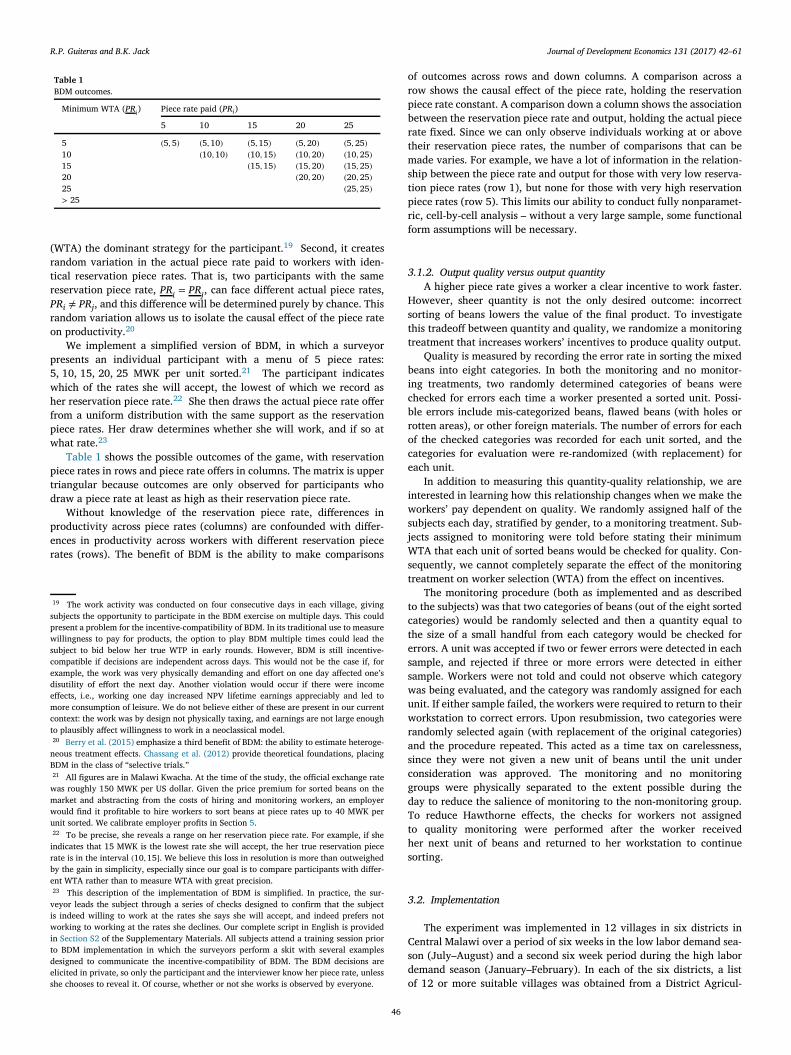
Table 1BDM outcomes.

Minimum WTA (PRi) Piece rate paid (PRi)

5 10 15 20 25

5 (5,5) (5,10) (5,15) (5,20) (5,25)10 (10,10) (10,15) (10,20) (10,25)15 (15,15) (15,20) (15,25)20 (20,20) (20,25)25 (25,25)> 25

(WTA) the dominant strategy for the participant.19 Second, it createsrandom variation in the actual piece rate paid to workers with iden-tical reservation piece rates. That is, two participants with the samereservation piece rate, PRi = PRj, can face different actual piece rates,PRi ≠ PRj, and this difference will be determined purely by chance. Thisrandom variation allows us to isolate the causal effect of the piece rateon productivity.20

We implement a simplified version of BDM, in which a surveyorpresents an individual participant with a menu of 5 piece rates:5, 10, 15, 20, 25 MWK per unit sorted.21 The participant indicateswhich of the rates she will accept, the lowest of which we record asher reservation piece rate.22 She then draws the actual piece rate offerfrom a uniform distribution with the same support as the reservationpiece rates. Her draw determines whether she will work, and if so atwhat rate.23

Table 1 shows the possible outcomes of the game, with reservationpiece rates in rows and piece rate offers in columns. The matrix is uppertriangular because outcomes are only observed for participants whodraw a piece rate at least as high as their reservation piece rate.

Without knowledge of the reservation piece rate, differences inproductivity across piece rates (columns) are confounded with differ-ences in productivity across workers with different reservation piecerates (rows). The benefit of BDM is the ability to make comparisons

19 The work activity was conducted on four consecutive days in each village, givingsubjects the opportunity to participate in the BDM exercise on multiple days. This couldpresent a problem for the incentive-compatibility of BDM. In its traditional use to measurewillingness to pay for products, the option to play BDM multiple times could lead thesubject to bid below her true WTP in early rounds. However, BDM is still incentive-compatible if decisions are independent across days. This would not be the case if, forexample, the work was very physically demanding and effort on one day affected one’sdisutility of effort the next day. Another violation would occur if there were incomeeffects, i.e., working one day increased NPV lifetime earnings appreciably and led tomore consumption of leisure. We do not believe either of these are present in our currentcontext: the work was by design not physically taxing, and earnings are not large enoughto plausibly affect willingness to work in a neoclassical model.20 Berry et al. (2015) emphasize a third benefit of BDM: the ability to estimate heteroge-neous treatment effects. Chassang et al. (2012) provide theoretical foundations, placingBDM in the class of “selective trials.”21 All figures are in Malawi Kwacha. At the time of the study, the official exchange ratewas roughly 150 MWK per US dollar. Given the price premium for sorted beans on themarket and abstracting from the costs of hiring and monitoring workers, an employerwould find it profitable to hire workers to sort beans at piece rates up to 40 MWK perunit sorted. We calibrate employer profits in Section 5.22 To be precise, she reveals a range on her reservation piece rate. For example, if sheindicates that 15 MWK is the lowest rate she will accept, the her true reservation piecerate is in the interval (10,15]. We believe this loss in resolution is more than outweighedby the gain in simplicity, especially since our goal is to compare participants with differ-ent WTA rather than to measure WTA with great precision.23 This description of the implementation of BDM is simplified. In practice, the sur-veyor leads the subject through a series of checks designed to confirm that the subjectis indeed willing to work at the rates she says she will accept, and indeed prefers notworking to working at the rates she declines. Our complete script in English is providedin Section S2 of the Supplementary Materials. All subjects attend a training session priorto BDM implementation in which the surveyors perform a skit with several examplesdesigned to communicate the incentive-compatibility of BDM. The BDM decisions areelicited in private, so only the participant and the interviewer know her piece rate, unlessshe chooses to reveal it. Of course, whether or not she works is observed by everyone.

of outcomes across rows and down columns. A comparison across arow shows the causal effect of the piece rate, holding the reservationpiece rate constant. A comparison down a column shows the associationbetween the reservation piece rate and output, holding the actual piecerate fixed. Since we can only observe individuals working at or abovetheir reservation piece rates, the number of comparisons that can bemade varies. For example, we have a lot of information in the relation-ship between the piece rate and output for those with very low reserva-tion piece rates (row 1), but none for those with very high reservationpiece rates (row 5). This limits our ability to conduct fully nonparamet-ric, cell-by-cell analysis – without a very large sample, some functionalform assumptions will be necessary.

3.1.2. Output quality versus output quantityA higher piece rate gives a worker a clear incentive to work faster.

However, sheer quantity is not the only desired outcome: incorrectsorting of beans lowers the value of the final product. To investigatethis tradeoff between quantity and quality, we randomize a monitoringtreatment that increases workers’ incentives to produce quality output.

Quality is measured by recording the error rate in sorting the mixedbeans into eight categories. In both the monitoring and no monitor-ing treatments, two randomly determined categories of beans werechecked for errors each time a worker presented a sorted unit. Possi-ble errors include mis-categorized beans, flawed beans (with holes orrotten areas), or other foreign materials. The number of errors for eachof the checked categories was recorded for each unit sorted, and thecategories for evaluation were re-randomized (with replacement) foreach unit.

In addition to measuring this quantity-quality relationship, we areinterested in learning how this relationship changes when we make theworkers’ pay dependent on quality. We randomly assigned half of thesubjects each day, stratified by gender, to a monitoring treatment. Sub-jects assigned to monitoring were told before stating their minimumWTA that each unit of sorted beans would be checked for quality. Con-sequently, we cannot completely separate the effect of the monitoringtreatment on worker selection (WTA) from the effect on incentives.

The monitoring procedure (both as implemented and as describedto the subjects) was that two categories of beans (out of the eight sortedcategories) would be randomly selected and then a quantity equal tothe size of a small handful from each category would be checked forerrors. A unit was accepted if two or fewer errors were detected in eachsample, and rejected if three or more errors were detected in eithersample. Workers were not told and could not observe which categorywas being evaluated, and the category was randomly assigned for eachunit. If either sample failed, the workers were required to return to theirworkstation to correct errors. Upon resubmission, two categories wererandomly selected again (with replacement of the original categories)and the procedure repeated. This acted as a time tax on carelessness,since they were not given a new unit of beans until the unit underconsideration was approved. The monitoring and no monitoringgroups were physically separated to the extent possible during theday to reduce the salience of monitoring to the non-monitoring group.To reduce Hawthorne effects, the checks for workers not assignedto quality monitoring were performed after the worker receivedher next unit of beans and returned to her workstation to continuesorting.

3.2. Implementation

The experiment was implemented in 12 villages in six districts inCentral Malawi over a period of six weeks in the low labor demand sea-son (July–August) and a second six week period during the high labordemand season (January–February). In each of the six districts, a listof 12 or more suitable villages was obtained from a District Agricul-

46

R.P. Guiteras and B.K. Jack Journal of Development Economics 131 (2017) 42–61

ture Extension Officer.24 We then randomly selected 2 villages fromeach district, one for implementation during the low labor demand sea-son and a second during the high labor demand season. Rather thanreturning to the same villages across seasons, we chose to work in dif-ferent villages in different seasons. This makes the worker pools notdirectly comparable across seasons, but even if we had returned to thesame villages, the pools would not have been the same since – in addi-tion to likely differences in selection into the study – learning, differ-ences in trust, etc., would have persisted across seasons. The villagewas informed of the activities approximately one week in advance andan open invitation was issued to attend the orientation and trainingsession on a Monday afternoon. Subjects who participated in the orien-tation session were registered and became eligible to participate in thesubsequent days’ activities.

During the orientation session, the bean sorting task was explainedand surveyors performed a skit to illustrate the BDM mechanism andshow subjects that truthful revelation of their minimum WTA was theirbest strategy. The distribution of possible piece rates was made clearduring the description of the task and the performance of the skit.Subjects were also informed that they would receive a participationfee of 50 MWK for each day they participated, plus their earningsfrom the day’s work.25 The participation fee was intended to offsetthe time costs of participants who showed up but were not awardeda contract. The information provided during the orientation sessionpresumably resulted in some selection out of the study by workerswith a reservation piece rate above the highest piece rate offered. Weargue that this selected sample is the relevant one for understandingthe determinants of productivity for the labor market activity that westudy.

Because of field capacity constraints, we limited the number of BDMparticipants on each day to 50. After the first three weeks of the firstdata collection period, the number was reduced to 40 to address imple-mentation challenges caused by the high acceptance rates of even lowpiece rate offers. On a given work day, if more than 40 (50) of sub-jects arrived by the pre-specified start time, a lottery was conductedto select 40 (50) participants. Those who were not selected were com-pensated for their time with a bar of soap. This constraint was oftenbinding: on average, 52.9 (s.d. 20.9) potential subjects arrived on timeand were eligible to participate in the lottery if there was one (48.5(s.d. 10.7) in the low season and 57.3 (s.d. 27.1) in the high season).A lottery was used on 15 of 24 days of the experiment in the lowlabor demand season, and on all 24 days in the high labor demandseason.

Conditional on attending the initial afternoon training session, weobserve attendance decisions for every subsequent work day, for a totalof four attendance observations per individual. Conditional on attend-ing in a given day and being selected to participate in BDM and the sur-vey, we also observe her reservation piece rate.26 Participants whoseBDM draw was greater than or equal to their stated reservation piecerate received a contract. For contracted workers, we observe the num-ber of bean units that a worker sorts and the quality for every unit

24 The villages were identified as locations where the collaborating NGO was not work-ing. They were also selected on a number of characteristics, including distance from thedistrict capital and distance from the road since these factors are likely to affect the func-tioning of labor markets in these villages.25 We note a tradeoff associated with offering a participation fee that is high relative tothe average earnings in the experiment. On the one hand, the participation fee may helpoffset selection into the experiment. On the other hand, if individuals have an incomegoal for the day (as in Farber (2005); Dupas and Robinson (2013)) or utility that is veryconcave in income, then the participation fee may dampen worker response to the piecerate. The target earnings model will dampen the response to the piece rate regardless ofthe participation fee, and reasonable utility functions are unlikely to generate curvaturesufficient for the participation fee to make a substantial difference.26 Individuals who participated in BDM in a previous session were given priority tomaximize the balance within the panel of observations. This priority status did not dependon whether they received a contract.

sorted. At the end of the work day, partially sorted units were paidaccording to the fraction of the unit sorted.27

A short survey was administered to every participant to collect basiccovariates, in particular those likely to be associated with the opportu-nity cost of time.28 The participation fee was contingent on the partic-ipant completing the survey.

We gathered additional qualitative data to provide context on theganyu market in Malawi. Specifically, we interviewed 53 workers and8 employers at trading posts and agri-processing centers in and aroundLilongwe.29 We targeted locations known to employ ganyu workers andasked questions pertaining both to the work conducted at the locationand to past ganyu contracts. The most commonly observed ganyu activ-ities among workers on the day of the interview was sorting ground-nuts, maize, soya and other beans, and offloading bags from trucksarriving at the trading posts and processing centers. About half of thesewere paid a time rate (55 percent) and half a piece rate (45 percent).Most (74 percent) said that their employer monitored the quality ofthe work, though the likelihood of monitoring was considerably lowerfor workers on piece rate than on time rate contracts (62.5 versus 82.8percent). Most often, workers report that monitoring is done by super-visors who observe work in process, though some monitoring appearsmore systematic, with random spot checks or an inspection stage to theprocess. Penalties for unsatisfactory performance are severe: workersreport having to do the entire task over again or losing out on the day’spay.

3.3. Descriptive statistics

3.3.1. Characteristics and participationKey characteristics of participants are described in Table 2, which

breaks the sample into the low and high seasons (six weeks per season).There were 689 total participants, 355 in the low labor season and 334in the high season. Individuals could work multiple days of the week,which results in an unbalanced individual panel by day with 1875observations, 1005 in the low season and 870 in the high season.30

Over 60 percent of the sample is female and between 20 and 30percent are from female-headed households. Effectively all participantswork in agriculture, and approximately two-thirds of households growbeans. Close to 40 percent of the sample report performing some casuallabor (ganyu) the previous week, and conditional on any ganyu, themean is 3.8 days. Because the study samples from different villages inthe low and high labor demand seasons, we report means and stan-dard deviations separately for each season. Some differences are statis-tically significant. Most notably, the daily wage reported for the mostrecent casual labor is significantly higher in the high labor demand sea-son. Individuals who join during the high season report slightly fewermonths per year of food shortage, suggesting that they are better off

27 Fifteen minutes before the end of the work day, enumerators stopped handing outunits for sorting, so most workers completed their final unit. Any proportional paymentswere estimated by the enumerators.28 Survey data were collected in two parts. The first, more comprehensive part, coveringbasic demographics and other time-invariant variables, was conducted only once witheach participant. That is, a subject who was selected to participate on a given day was notadministered this part of the survey if she had participated (and therefore been surveyed)on a previous day. The second part was a brief set of questions on the subject’s potentialalternative activities for that day and participants’ expected output that day. In both cases,the survey was conducted regardless of the outcome of the BDM experiment. However,for logistical reasons, both were administered after the BDM experiment was conductedand the results were known, so it is possible that the responses were affected by the resultof the experiment.29 This qualitative data collection was completed in June 2017, as part of a revision tothis paper.30 Covariate balance for the piece rate draws and the monitoring treatment is shown inTable S1. Because we see some imbalance, we include controls in selected specificationsin all of our main analyses.

47

R.P. Guiteras and B.K. Jack Journal of Development Economics 131 (2017) 42–61

Table 2Descriptive statistics for participants.

All(1) Low Season(2) High Season(3) Diff.(4)

Number of participants 689 355 334Number of daily observations 1875 1005 870Female 0.665

(0.472)0.690(0.463)

0.638(0.481)

−0.052***

[0.018]Age 34.9

(13.6)34.6(13.2)

35.2(14.1)

0.6[0.6]

Number of adults in household 3.10(1.68)

3.16(1.59)

3.04(1.78)

−0.12**

[0.06]Years of education 4.23

(3.27)3.91(3.35)

4.57(3.16)

0.66***

[0.13]Female headed household 0.252

(0.434)0.201(0.401)

0.305(0.461)

0.104***

[0.017]Participated in ganyu in last week 0.38

(0.48)0.33(0.47)

0.42(0.49)

0.09***

[0.02]Days of ganyu last week, conditional on positive 3.77

(2.07)4.22(2.15)

3.39(1.93)

−0.83***

[0.13]Daily wage from recent ganyu (MKW) 302.6

(329.9)257.7(178.7)

344.6(420.9)

86.9***

[13.1]Household produces maize 0.999

(0.038)1.000(0.000)

0.997(0.055)

−0.003[0.002]

Household produces beans 0.657(0.475)

0.686(0.464)

0.627(0.484)

−0.059***

[0.018]Typical per year months without adequate food 3.35

(2.27)3.56(2.34)

3.13(2.16)

−0.43***

[0.09]Alternative activity: housework 0.152

(0.360)0.216(0.411)

0.079(0.270)

−0.137***

[0.016]Alternative activity: other ganyu 0.200

(0.400)0.257(0.437)

0.135(0.342)

−0.122***

[0.018]Alternative activity: work own land 0.408

(0.492)0.269(0.444)

0.569(0.495)

0.300***

[0.022]Alternative activity: work own business 0.084

(0.277)0.049(0.216)

0.124(0.330)

0.075***

[0.013]

Notes: this table presents means of participants’ characteristics during the low and high season, with standard devia-tions in parentheses, as well as differences in means, with the standard error of the estimated difference in brackets. *

p < 0.10, ** p < 0.05, *** p < 0.01.

than participants in the low season.31 In the high season, workers areless likely to list housework as one of their alternative activities for theday and more likely to list working their own land.32

Several factors may contribute to the observed differences acrosslabor seasons. First, the underlying characteristics of the villages vis-ited may differ across seasons. Although our villages were randomlyassigned to season, given our small number of villages (12) we can-not appeal to the law of large numbers to argue that the villages arelikely to be well-balanced. Second, different types of individuals mayhave selected into the study in each season, explaining differences inaverage participant age or other income sources. Finally, seasonal vari-ation in labor demand and productive activities may explain differencesin reported casual labor wages and outside options on the day of datacollection.33

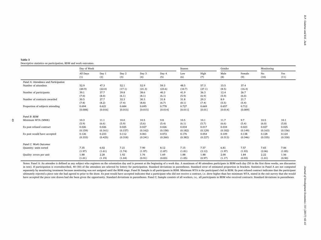
Table 3 provides descriptive statistics on participation, BDM out-comes, and work outcomes. In Panel A, we summarize attendance andparticipation rates overall (column 1) and by day (columns 2–5), bylabor season (columns 6 and 7), and by participant gender (columns 8and 9). On average, the number of attendees is increasing through the

31 Households are more likely to have run out of food in January (high season) than inJuly (low season), which suggests that this difference is not due to the salience of foodshortages during food short months.32 Summary statistics on a broader set of survey measures are reported in Table S2 ofthe Supplementary Materials.33 These explanations are not mutually exclusive. For example, differences in incomesources may be due both to self selection and underlying differences in the villages.Because of the difficulty distinguishing among them, we do not emphasize direct com-parisons of results across labor season.

week, with more attendees during the high season. The average shareof registered subjects attending each day is lower for the high season,due both to fewer repeat workers during this period and to use of thelottery to limit the number of participants in all weeks. Individuals inthe low labor season work an average of 2.8 days while individuals inthe high season work an average of 2.6 days out of the possible 4 workdays.

3.3.2. Willingness to acceptPanel B of Table 3 provides summary statistics on behavior in BDM.

The first row shows the mean minimum WTA revealed in BDM, for thesame categories as Panel A, and additionally by monitoring treatment(columns 10 and 11). The salient facts are that mean minimum WTAfalls after the first day, and the mean minimum WTA for women isapproximately 2 MWK lower than for men.34 We do not observe sig-nificant differences by season or by monitoring treatment. Fig. 1 showsthe share of participants accepting each of the 5 piece rates.35 Themost striking fact is that most participants are willing to accept verylow piece rates: over 60 percent of participants accept a piece rate of10 MWK per unit, for which expected daily earnings would be approx-imately 70 MWK, plus the 50 MWK show up fee.36 This is consistent

34 For correlations between WTA and other characteristics, see Table S3, which reportsthe pairwise correlation between outcomes (WTA, quantity and quality) and survey mea-sures.35 The acceptance rates plotted in Fig. 1 are provided in Table S4.36 These calculations consider only the acceptance of piece rates revealed by the BDM.Attrition or selective attendance might cause us to over-estimate acceptance rates ifhigh minimum WTA individuals attended fewer work days. We note that, conditional onattending any work days, minimum WTA is correlated with the number of days attended.

48

R.P.Guiterasand

B.K.JackJournalofD

evelopmentEconom

ics131(2017)

42–61

Table 3Descriptive statistics on participation, BDM and work outcomes.

Day of Week Season Gender Monitoring

All Days Day 1 Day 2 Day 3 Day 4 Low High Male Female No Yes(1) (2) (3) (4) (5) (6) (7) (8) (9) (10) (11)

Panel A: Attendance and ParticipationNumber of attendees 52.9

(20.9)47.3(22.0)

52.1(17.1)

52.9(21.3)

59.3(23.6)

48.5(10.7)

57.3(27.1)

15.5(8.5)

37.4(16.4)

Number of participants 39.1(7.0)

37.7(8.0)

39.8(6.1)

38.6(8.1)

40.3(6.1)

41.9(5.9)

36.3(6.9)

12.4(5.9)

26.7(6.0)

Number of contracts awarded 30.5(7.8)

27.7(8.2)

32.3(7.4)

30.3(8.8)

31.8(6.7)

31.8(8.1)

29.3(7.4)

8.9(5.5)

21.7(5.4)

Proportion of subjects attending 0.694[0.008]

0.621[0.016]

0.684[0.015]

0.695[0.015]

0.778[0.014]

0.727[0.011]

0.669[0.01]

0.657[0.014]

0.712[0.009]

Panel B: BDMMinimum WTA (MWK) 10.3

(5.9)11.1(6.6)

10.0(5.9)

10.5(5.6)

9.8(5.4)

10.5(6.1)

10.1(5.7)

11.7(6.6)

9.7(5.4)

10.5(6.0)

10.1(5.8)

Ex post refused contract 0.026(0.159)

0.026(0.161)

0.025(0.157)

0.027(0.162)

0.026(0.158)

0.034(0.182)

0.017(0.129)

0.034(0.182)

0.023(0.149)

0.027(0.163)

0.025(0.156)

Ex post would have accepted 0.126(0.333)

0.233(0.425)

0.112(0.318)

0.061(0.241)

0.072(0.260)

0.176(0.382)

0.054(0.227)

0.109(0.313)

0.138(0.346)

0.128(0.335)

0.124(0.330)

Panel C: Work OutcomesQuantity: units sorted 7.35

(1.97)6.02(1.61)

7.21(1.74)

7.90(1.97)

8.12(1.87)

7.15(1.81)

7.57(2.12)

6.81(1.97)

7.57(1.93)

7.65(2.06)

7.06(1.85)

Quality: errors per unit 1.88(1.01)

2.20(1.19)

1.92(1.04)

1.76(0.91)

1.69(0.83)

1.88(1.05)

1.88(0.97)

2.00(1.17)

1.84(0.93)

2.22(1.01)

1.56(0.90)

Notes: Panel A: An attendee is defined as any subject who registers on the orientation day and is present at the beginning of a work day. A maximum of 40 attendees participate in BDM each day (50 in the first three weeks, see discussionin text). If participation is oversubscribed, 40 (50) of the attendees are selected by lottery for participation. Standard deviations in parentheses. Standard error of estimated proportion in brackets. Statistics in Panel A are not computedseparately by monitoring treatment because monitoring was not assigned until the BDM stage. Panel B: Sample is all participants in BDM. Minimum WTA is the participant’s bid in BDM. Ex post refused contract indicates that the participantultimately rejected a piece rate she had agreed to prior to the draw. Ex post would have accepted indicates that a participant who did not receive a contract, i.e. drew higher than her minimum WTA, stated in the exit survey that she wouldhave accepted the piece rate drawn had she been given the opportunity. Standard deviations in parentheses. Panel C: Sample consists of all workers, i.e,. all participants in BDM who received contracts. Standard deviations in parentheses.

49

R.P. Guiteras and B.K. Jack Journal of Development Economics 131 (2017) 42–61

Fig. 1. CDFs of minimum piece rate accepted. Notes: These figures plot the share of participants who agree to work at each of the given piece rates, i.e., those participants whose bidsin BDM were as high or higher than that piece rate.

with the high rate of labor force participation even at very low dailywages observed by Goldberg (2016). Conditional on working, meandaily earnings were over 170 MWK, which exceeds average daily wagesreported in the 2004 IHS and induced over 90 percent of the adult pop-ulation in Goldberg’s study to agree to work.37

The bottom two rows of Panel B summarize “mistakes” in theBDM procedure. Very few participants (<3 percent) refused a drawnprice that they had accepted in their BDM decisions. A larger share(13 percent) state ex-post that they would have been willing to accepta drawn rate that they had rejected in their BDM decisions. The ex-postrefusal rate declines throughout the week, consistent with participants

Specifically, a 5 MWK increase in minimum WTA is associated with 0.25–0.4 fewer daysin attendance. However, acceptance rates of low piece rates remains high even if we takethe extreme stance and interpret decisions not to attend as rejections all offered piecerates. In this scenario, 43 percent accept an offer of 10 MWK. Alternatively, if we assumethat those who chose not to attend all days have a stable minimum WTA equal to theirhighest observed minimum WTA in the BDM, then 53 percent accept an offer of 10 MWK.Importantly, the attendance decision is unrelated to the previous day’s randomly drawnpiece rate or to the previous day’s monitoring treatment. We further note that the decisionof how to treat missing minimum WTA observations will only change our interpretationof selection effects on productivity if the workers with high minimum WTA who choosenot to attend all days (or at all) also have high productivity in the bean sorting task.37 Workers sorted an average of 7.35 units per day (Table 3). Workers reported thatthey expected to sort an average of 6.74 units per day (Table S2).

learning that stating one’s true minimum WTA was their best strategy.It also declines across weeks (noisily, not reported), which suggests thatsurveyors improved at communicating the optimal strategy to partici-pants. Of course, the participant’s statement that she would have beenwilling to accept at a previously rejected rate is purely hypothetical andindividuals may have wished to express a willingness to work in theirresponses to this non-binding question.

3.3.3. Quantity and quality of worker outputThe primary measures of productivity, number of units sorted per

day (Y) and average number of errors per unit (Q), are summarized inPanel C of Table 3.38 The mean number of units sorted per day acrossall days is 7.35 (s.d. 1.97), which is increasing throughout the week,and the mean number of errors per unit is 1.88 (s.d. 1.01). The quan-tity of output is lower (0.59 fewer units per day) and the quality ofoutput is higher (0.66 fewer errors per unit) in the monitoring treat-ment, suggested that workers sorted more carefully and therefore moreslowly in the monitoring treatment. Females sort 0.76 more units perday than men, and commit slightly fewer errors per unit (0.16). Thisco-movement of quantity and quality is observed for several covariates

38 Q is recorded the first time the workers bring a unit of sorted beans to the enumerator,before they have been instructed to correct any errors above the threshold.

50

R.P. Guiteras and B.K. Jack Journal of Development Economics 131 (2017) 42–61

Table 4Predictors of minimum willingness to accept.

Pooled Random Effects Fixed Effects

(1) (2) (3) (4) (5)

Monitoring −0.431(0.269)

−0.546**

(0.265)−0.297(0.221)

−0.333(0.221)

−0.189(0.235)

High season −0.780**

(0.377)−0.223(0.399)

−0.901**

(0.386)−0.362(0.408)

Female −2.321***

(0.449)−2.662***

(0.484)−2.635***

(0.453)−2.875***

(0.490)Second day −0.904***

(0.343)−0.849**

(0.342)−0.998***

(0.319)−0.914***

(0.321)−1.040***

(0.330)Third day −0.326

(0.353)−0.303(0.349)

−0.177(0.336)

−0.149(0.335)

−0.108(0.352)

Fourth day −1.086***

(0.351)−1.095***

(0.352)−1.072***

(0.339)−1.048***

(0.340)−1.077***

(0.353)

Indiv. Controls No Yes No Yes NoMean Dep. Var. 10.320 10.320 10.320 10.320 10.320SD Dep. Var. 5.899 5.899 5.899 5.899 5.899Num. of participants 682 682 682 682 682Num. of observations 1857 1857 1857 1857 1857

Notes: this table presents regressions of minimum willingness to accept (WTA) on season, monitoring, whetherthe participant was female, and day-of-week fixed effects, with the first day as the omitted category. Columns(1)–(2) pool data across participants and days. Columns (3)–(4) include random participant effects. Column (5)includes participant fixed effects. Columns (2) and (4) control for individual covariates (age, number of adults inhousehold, number of other household members participating, years of education, whether the head of householdis female, days of ganyu in the previous week and month, reported daily wage from recent ganyu, householdtype of agricultural output (beans, tobacco, other), typical number of months per year without adequate food,household sources of income (ganyu, selling food products, selling beer, selling crafts, small shop), alternativeactivity for that day (housework, other ganyu, work own land, work in own business), number of units participantexpects to sort). All regressions include district fixed effects, although in column (5) these are absorbed by theindividual fixed effects. Standard errors clustered by participant. * p < 0.10, ** p < 0.05, *** p < 0.01.

(see Table S3), consistent with our model’s single productivity parame-ter for quality and quantity.

4. Empirical results

We present our empirical strategy and results together. Our threeoutcome measures are minimum WTA as measured by BDM, quantityof output measured by the number of units of beans sorted per day,and quality of output measured by the number of errors per unit. Wefirst discuss which covariates predict minimum WTA. Second, we esti-mate the determinants of both quantity and quality of output, separat-ing selection – minimum WTA, conditional on the piece rate – fromincentive effects, which are associated both with the randomly deter-mined piece rate and with the quality monitoring treatment. Finally,we estimate differences in minimum WTA and productivity determi-nants between men and women.

4.1. Determinants of minimum WTA

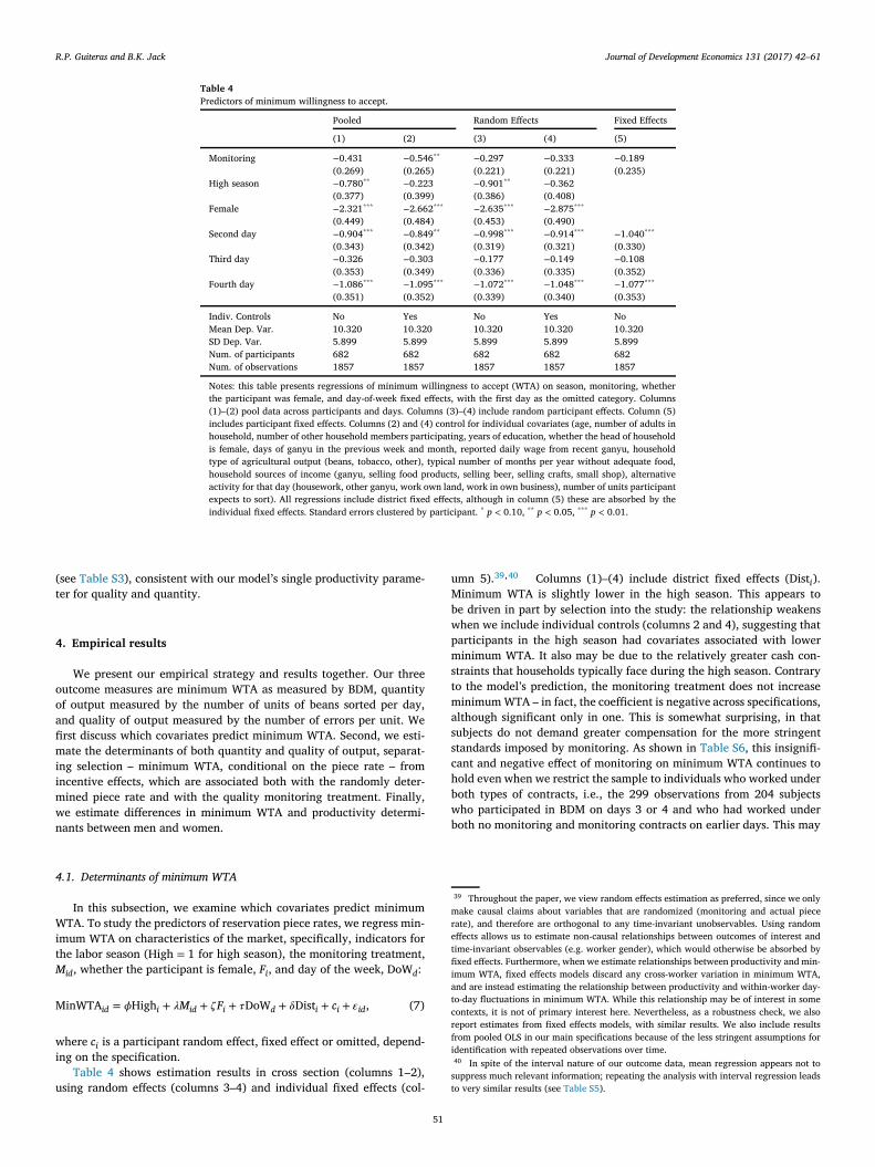
In this subsection, we examine which covariates predict minimumWTA. To study the predictors of reservation piece rates, we regress min-imum WTA on characteristics of the market, specifically, indicators forthe labor season (High = 1 for high season), the monitoring treatment,Mid, whether the participant is female, Fi, and day of the week, DoWd:

MinWTAid = 𝜙Highi + 𝜆Mid + 𝜁Fi + 𝜏DoWd + 𝛿Disti + ci + 𝜀id, (7)

where ci is a participant random effect, fixed effect or omitted, depend-ing on the specification.

Table 4 shows estimation results in cross section (columns 1–2),using random effects (columns 3–4) and individual fixed effects (col-

umn 5).39,40 Columns (1)–(4) include district fixed effects (Disti).Minimum WTA is slightly lower in the high season. This appears tobe driven in part by selection into the study: the relationship weakenswhen we include individual controls (columns 2 and 4), suggesting thatparticipants in the high season had covariates associated with lowerminimum WTA. It also may be due to the relatively greater cash con-straints that households typically face during the high season. Contraryto the model’s prediction, the monitoring treatment does not increaseminimum WTA – in fact, the coefficient is negative across specifications,although significant only in one. This is somewhat surprising, in thatsubjects do not demand greater compensation for the more stringentstandards imposed by monitoring. As shown in Table S6, this insignifi-cant and negative effect of monitoring on minimum WTA continues tohold even when we restrict the sample to individuals who worked underboth types of contracts, i.e., the 299 observations from 204 subjectswho participated in BDM on days 3 or 4 and who had worked underboth no monitoring and monitoring contracts on earlier days. This may

39 Throughout the paper, we view random effects estimation as preferred, since we onlymake causal claims about variables that are randomized (monitoring and actual piecerate), and therefore are orthogonal to any time-invariant unobservables. Using randomeffects allows us to estimate non-causal relationships between outcomes of interest andtime-invariant observables (e.g. worker gender), which would otherwise be absorbed byfixed effects. Furthermore, when we estimate relationships between productivity and min-imum WTA, fixed effects models discard any cross-worker variation in minimum WTA,and are instead estimating the relationship between productivity and within-worker day-to-day fluctuations in minimum WTA. While this relationship may be of interest in somecontexts, it is not of primary interest here. Nevertheless, as a robustness check, we alsoreport estimates from fixed effects models, with similar results. We also include resultsfrom pooled OLS in our main specifications because of the less stringent assumptions foridentification with repeated observations over time.40 In spite of the interval nature of our outcome data, mean regression appears not tosuppress much relevant information; repeating the analysis with interval regression leadsto very similar results (see Table S5).

51

R.P. Guiteras and B.K. Jack Journal of Development Economics 131 (2017) 42–61

Fig. 2. Selection and Incentives. Notes: these figures plot estimated differences from regressions of either quantity (units sorted per day) or quality (errors per unit) on interactedquadratics in minimum willingness to pay and the piece rate (draw), interacted with monitoring, controlling nonparametrically for gender, season, district, day in the village and workerrandom effects. The estimated differences are relative to no monitoring, a minimum WTA of 5 MWK per unit sorted, and a piece rate of 5 MWK per unit sorted. The x-axis is the piecerate (draw), so each line compares workers who have the same minimum WTA but earn different piece rates.

reflect a preference for more complete contracts, or inattention to thecontractual details at the time of bidding.

Minimum WTA falls over the course of the week, which cannot beexplained solely by selection given the robustness to individual fixedeffects (column 5). Minimum WTA is about 1 MWK higher on the firstday than on later days in the week, relative to a mean of 10 MWK inthe sample. Some of the variation in minimum WTA within-individual iscorrelated with the self-reported outside option, as shown in Table S7.Specifically, individuals who report that their alternative activity forthe day was associated with cash income (other casual labor, workingown business) have lower reservation rates, as do those who wouldhave worked on their own farms. Importantly for identification in thenext sections, minimum WTA is not affected by treatments on the pre-vious day (for subjects who attend on multiple days), i.e., the piece ratedraw and the monitoring treatment do not affect BDM behavior on thesubsequent day.

4.2. Determinants of productivity

Next, we investigate the role of both selection into the contract andthe incentives provided by the contract on worker productivity. Thethought experiment, as described in Section 3.1.1, is to first compare

workers with different minimum WTA who receive the same randompiece rates, and second to compare workers with the same minimumWTA who receive different random piece rates. With a very large sam-ple, we could do this completely nonparametrically, e.g. by comparingoutcomes for each cell in Table 1. However, in our finite sample, somecell sizes are very small, requiring us to make some functional formassumptions. The basic intuition is unchanged: by controlling for thepiece rate, we isolate the selection channel; by controlling for minimumWTA, we isolate the direct effect of incentives on productivity. Theselatter effects are due solely to changes in the worker’s effort choice inresponse to a change in the piece rate or monitoring of output quality,both of which are randomized.41

We begin with a descriptive summary of the findings. As a mid-dle ground between flexibility and precision, we estimate a parametricmodel with quadratics in minimum WTA and the piece rate, their inter-action, all interacted with the monitoring treatment. Specifically, weestimate

41 Although monitoring is randomized, it is not random conditional on minimum WTA,since BDM participants announced their minimum WTA knowing whether or not theywere assigned to the monitoring group. As noted in Section 4.1, we do not observe thatbeing assigned to monitoring has a significant effect on stated minimum WTA.

52

R.P. Guiteras and B.K. Jack Journal of Development Economics 131 (2017) 42–61

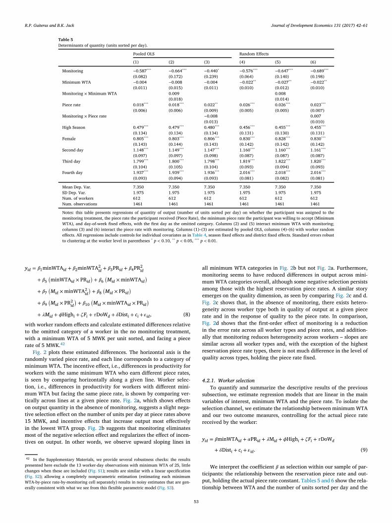
Table 5Determinants of quantity (units sorted per day).

Pooled OLS Random Effects

(1) (2) (3) (4) (5) (6)

Monitoring −0.587***

(0.082)−0.664***

(0.172)−0.440*

(0.239)−0.576***

(0.064)−0.647***

(0.140)−0.689***

(0.198)Minimum WTA −0.004

(0.011)−0.008(0.015)

−0.004(0.011)

−0.022**

(0.010)−0.027**

(0.012)−0.022**

(0.010)Monitoring × Minimum WTA 0.009

(0.018)0.008(0.014)

Piece rate 0.018***

(0.006)0.018***

(0.006)0.022**

(0.009)0.026***

(0.005)0.026***

(0.005)0.023***

(0.007)Monitoring × Piece rate −0.008

(0.013)0.007(0.010)

High Season 0.479***

(0.134)0.479***

(0.134)0.480***

(0.134)0.456***

(0.131)0.455***

(0.130)0.455***

(0.131)Female 0.805***

(0.143)0.803***

(0.144)0.806***

(0.143)0.830***

(0.142)0.828***

(0.142)0.830***

(0.142)Second day 1.148***

(0.097)1.149***

(0.097)1.147***

(0.098)1.160***

(0.087)1.160***

(0.087)1.161***

(0.087)Third day 1.799***

(0.104)1.800***

(0.105)1.798***

(0.104)1.819***

(0.093)1.822***

(0.094)1.820***

(0.093)Fourth day 1.937***

(0.093)1.939***

(0.094)1.936***

(0.093)2.016***

(0.081)2.018***

(0.082)2.016***

(0.081)

Mean Dep. Var. 7.350 7.350 7.350 7.350 7.350 7.350SD Dep. Var. 1.975 1.975 1.975 1.975 1.975 1.975Num. of workers 612 612 612 612 612 612Num. observations 1461 1461 1461 1461 1461 1461

Notes: this table presents regressions of quantity of output (number of units sorted per day) on whether the participant was assigned to themonitoring treatment, the piece rate the participant received (Piece Rate), the minimum piece rate the participant was willing to accept (MinimumWTA), and day-of-week fixed effects, with the first day as the omitted category. Columns (2) and (5) interact minimum WTA with monitoring;columns (3) and (6) interact the piece rate with monitoring. Columns (1)–(3) are estimated by pooled OLS, columns (4)–(6) with worker randomeffects. All regressions include controls for individual covariates as in Table 4, season fixed effects and district fixed effects. Standard errors robustto clustering at the worker level in parentheses * p < 0.10, ** p < 0.05, *** p < 0.01.

yid = 𝛽1minWTAid + 𝛽2minWTA2id + 𝛽3PRid + 𝛽4PR2

id

+ 𝛽5(minWTAid × PRid

)+ 𝛽6

(Mid × minWTAid

)+ 𝛽7

(Mid × minWTA2

id)+ 𝛽8

(Mid × PRid

)+ 𝛽9

(Mid × PR2

id)+ 𝛽10

(Mid × minWTAid × PRid

)+ 𝜆Mid + 𝜙Highi + 𝜁Fi + 𝜏DoWd + 𝛿Disti + ci +𝜀id, (8)

with worker random effects and calculate estimated differences relativeto the omitted category of a worker in the no monitoring treatment,with a minimum WTA of 5 MWK per unit sorted, and facing a piecerate of 5 MWK.42

Fig. 2 plots these estimated differences. The horizontal axis is therandomly varied piece rate, and each line corresponds to a category ofminimum WTA. The incentive effect, i.e., differences in productivity forworkers with the same minimum WTA who earn different piece rates,is seen by comparing horizontally along a given line. Worker selec-tion, i.e., differences in productivity for workers with different mini-mum WTA but facing the same piece rate, is shown by comparing ver-tically across lines at a given piece rate. Fig. 2a, which shows effectson output quantity in the absence of monitoring, suggests a slight nega-tive selection effect on the number of units per day at piece rates above15 MWK, and incentive effects that increase output most effectivelyin the lowest WTA group. Fig. 2b suggests that monitoring eliminatesmost of the negative selection effect and regularizes the effect of incen-tives on output. In other words, we observe upward sloping lines in

42 In the Supplementary Materials, we provide several robustness checks: the resultspresented here exclude the 13 worker-day observations with minimum WTA of 25, littlechanges when these are included (Fig. S1); results are similar with a linear specification(Fig. S2); allowing a completely nonparametric estimation (estimating each minimumWTA-by-piece rate-by-monitoring cell separately) results in noisy estimates that are gen-erally consistent with what we see from this flexible parametric model (Fig. S3).

all minimum WTA categories in Fig. 2b but not Fig. 2a. Furthermore,monitoring seems to have reduced differences in output across mini-mum WTA categories overall, although some negative selection persistsamong those with the highest reservation piece rates. A similar storyemerges on the quality dimension, as seen by comparing Fig. 2c and d.Fig. 2c shows that, in the absence of monitoring, there exists hetero-geneity across worker type both in quality of output at a given piecerate and in the response of quality to the piece rate. In comparison,Fig. 2d shows that the first-order effect of monitoring is a reductionin the error rate across all worker types and piece rates, and addition-ally that monitoring reduces heterogeneity across workers – slopes aresimilar across all worker types and, with the exception of the highestreservation piece rate types, there is not much difference in the level ofquality across types, holding the piece rate fixed.

4.2.1. Worker selectionTo quantify and summarize the descriptive results of the previous

subsection, we estimate regression models that are linear in the mainvariables of interest, minimum WTA and the piece rate. To isolate theselection channel, we estimate the relationship between minimum WTAand our two outcome measures, controlling for the actual piece ratereceived by the worker:

yid = 𝛽minWTAid + 𝛼PRid + 𝜆Mid + 𝜙Highi + 𝜁Fi + 𝜏DoWd

+ 𝛿Disti + ci + 𝜀id. (9)

We interpret the coefficient 𝛽 as selection within our sample of par-ticipants: the relationship between the reservation piece rate and out-put, holding the actual piece rate constant. Tables 5 and 6 show the rela-tionship between WTA and the number of units sorted per day and the

53

R.P. Guiteras and B.K. Jack Journal of Development Economics 131 (2017) 42–61

Table 6Determinants of quality (errors per unit sorted).

Pooled OLS Random Effects

(1) (2) (3) (4) (5) (6)

Monitoring −0.647***

(0.045)−0.575***

(0.097)−0.744***

(0.144)−0.614***

(0.043)−0.561***

(0.092)−0.722***

(0.137)Minimum WTA −0.005

(0.006)−0.001(0.008)

−0.005(0.006)

−0.003(0.006)

−0.000(0.008)

−0.003(0.006)

Monitoring × Minimum WTA −0.008(0.010)

−0.006(0.009)

Piece rate 0.009**

(0.004)0.009**

(0.004)0.006(0.006)

0.009**

(0.004)0.009**

(0.004)0.006(0.006)

Monitoring × Piece rate 0.006(0.008)

0.006(0.008)

High Season −0.039(0.063)

−0.038(0.063)

−0.039(0.063)

−0.050(0.065)

−0.050(0.065)

−0.051(0.066)

Female −0.258***

(0.072)−0.257***

(0.072)−0.259***

(0.072)−0.256***

(0.075)−0.255***

(0.075)−0.257***

(0.075)Second day −0.275***

(0.076)−0.275***

(0.076)−0.274***

(0.076)−0.293***

(0.076)−0.293***

(0.076)−0.292***

(0.076)Third day −0.414***

(0.073)−0.415***

(0.074)−0.413***

(0.073)−0.444***

(0.072)−0.445***

(0.072)−0.443***

(0.072)Fourth day −0.464***

(0.073)−0.466***

(0.073)−0.464***

(0.073)−0.491***

(0.073)−0.493***

(0.074)−0.491***

(0.073)

Mean Dep. Var. 1.883 1.883 1.883 1.883 1.883 1.883SD Dep. Var. 1.013 1.013 1.013 1.013 1.013 1.013Num. of workers 612 612 612 612 612 612Num. observations 1461 1461 1461 1461 1461 1461

Notes: this table presents regressions of quality of output (number of errors per unit) on whether the participant was assigned tothe monitoring treatment, the piece rate the participant received (Piece Rate), the minimum piece rate the participant was willingto accept (Minimum WTA), and day-of-week fixed effects, with the first day as the omitted category. Columns (2) and (5) interactminimum WTA with monitoring; columns (3) and (6) interact the piece rate with monitoring. Columns (1)–(3) are estimated by pooledOLS, columns (4)–(6) with worker random effects. All regressions include controls for individual covariates as in Table 4, season fixedeffects and district fixed effects. Standard errors robust to clustering at the worker level in parentheses * p < 0.10, ** p < 0.05, ***

p < 0.01.

number of errors per unit, respectively.43 Column (1) is estimated bypooled OLS, and column (4) by worker random effects.44 With respectto quantity, we observe slightly negative selection in some specifica-tions: after controlling for the worker incentive provided by the piecerate (PRid), the monitoring treatment and the day of the week, mini-mum WTA is negatively related to quantity of output in the randomeffects model (columns 4–6, Table 5), though the size of the coefficientis small (a 10 MWK increase in minimum WTA lowers the number ofunits sorted per day by 0.20–0.30, relative to a mean of 7.4 units) and inthe pooled OLS specification (columns 4–6, Table 5) is close to zero andstatistically insignificant. The same specification with number of errorsper unit as the dependent variable shows no significant relationshipbetween minimum WTA and quality of output, though the coefficienton minimum WTA is consistently negative (Table 6).

4.2.2. IncentivesBDM randomly assigns the piece rate paid among those who work,

so it is straightforward to test the causal effect of incentives on produc-tivity using Equation (9). Since we can control for minimum WTA, andthe piece rate is (conditionally) random, we can interpret the coefficient𝛼 causally as the incentive effect of the piece rate.

43 While we present and discuss quantity and quality results separately, it is importantto remember that they are jointly determined by the worker. That is, we should not thinkof determinants of quantity as operating with quality held fixed, nor vice versa.44 Fixed effects estimates are provided in Tables S8 and S9. We control for covariatesas listed in Table 4; specifications without controls are provided in Tables S10 and S11.Finally, we provide estimates using data only from the first day, to limit potential biasfrom attrition correlated with treatment (Tables S12 and S13). The results are qualita-tively similar, although with less precision – for example, the effect of the price draw isno longer statistically significant.

Table 7Predictors of willingness to accept differential effects by gender.

Pooled Random Effects

(1) (2) (3) (4)

MonitoringAmong Men −0.887

(0.574)−0.900(0.559)

−0.622(0.439)

−0.650(0.433)

Among Women −0.223(0.288)

−0.385(0.289)

−0.155(0.252)

−0.193(0.255)

High SeasonAmong Men −0.234

(0.790)−0.113(0.764)

−0.423(0.793)

−0.268(0.772)

Among Women −1.029**

(0.415)−0.282(0.449)

−1.126***

(0.427)−0.411(0.463)

Female Level Effect −2.259***

(0.744)−2.836***

(0.772)−2.514***

(0.729)−3.031***

(0.753)Indiv. Controls No Yes No YesMean Dep. Var. 10.320 10.320 10.320 10.320SD Dep. Var. 5.899 5.899 5.899 5.899Num. of participants 682 682 682 682Num. of observations 1857 1857 1857 1857

Notes: this table presents differential effects by gender of season and monitoring onminimum WTA (MWK) per unit sorted. Additional regressors not reported: day-of-week fixed effects, district fixed effects, and, where noted, individual covariates asin Table 6. Columns (1)–(2) pool data across participants and days. Columns (3)–(4)include random participant effects. Standard errors are clustered by participant.* p < 0.10, ** p < 0.05, *** p < 0.01.

Table 5 shows the effect of the piece rate on quantity of output,controlling for the worker’s reservation piece rate. Our basic specifica-tion is estimated by pooled OLS in column (1) and with worker randomeffects in column (4). Increasing the piece rate by 10 MWK increases thenumber of units sorted per day by between 0.18 and 0.26 units, relative

54

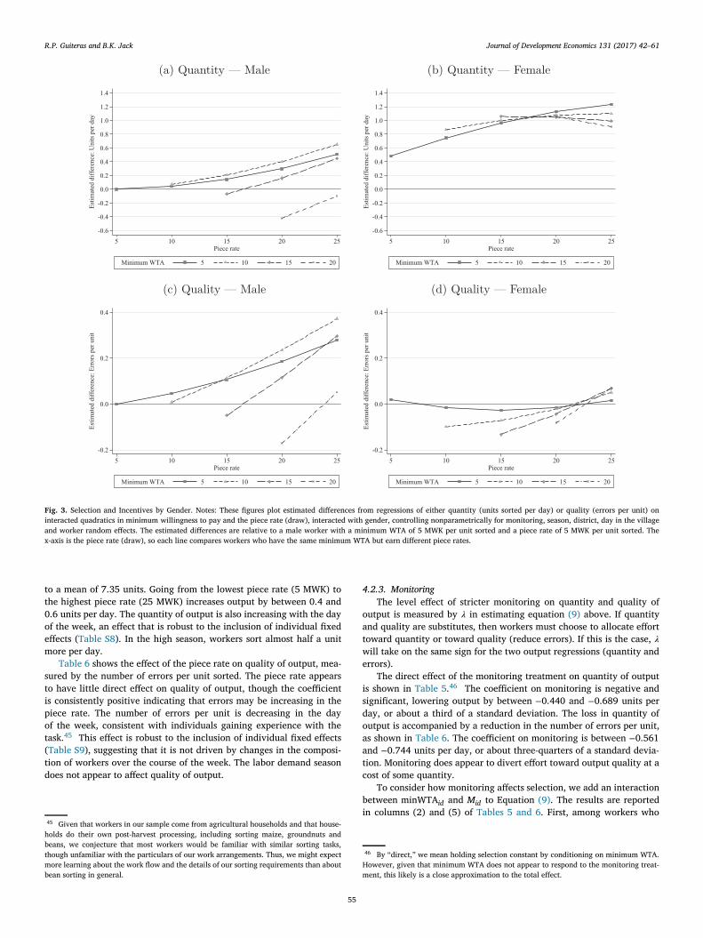
R.P. Guiteras and B.K. Jack Journal of Development Economics 131 (2017) 42–61

Fig. 3. Selection and Incentives by Gender. Notes: These figures plot estimated differences from regressions of either quantity (units sorted per day) or quality (errors per unit) oninteracted quadratics in minimum willingness to pay and the piece rate (draw), interacted with gender, controlling nonparametrically for monitoring, season, district, day in the villageand worker random effects. The estimated differences are relative to a male worker with a minimum WTA of 5 MWK per unit sorted and a piece rate of 5 MWK per unit sorted. Thex-axis is the piece rate (draw), so each line compares workers who have the same minimum WTA but earn different piece rates.

to a mean of 7.35 units. Going from the lowest piece rate (5 MWK) tothe highest piece rate (25 MWK) increases output by between 0.4 and0.6 units per day. The quantity of output is also increasing with the dayof the week, an effect that is robust to the inclusion of individual fixedeffects (Table S8). In the high season, workers sort almost half a unitmore per day.

Table 6 shows the effect of the piece rate on quality of output, mea-sured by the number of errors per unit sorted. The piece rate appearsto have little direct effect on quality of output, though the coefficientis consistently positive indicating that errors may be increasing in thepiece rate. The number of errors per unit is decreasing in the dayof the week, consistent with individuals gaining experience with thetask.45 This effect is robust to the inclusion of individual fixed effects(Table S9), suggesting that it is not driven by changes in the composi-tion of workers over the course of the week. The labor demand seasondoes not appear to affect quality of output.

45 Given that workers in our sample come from agricultural households and that house-holds do their own post-harvest processing, including sorting maize, groundnuts andbeans, we conjecture that most workers would be familiar with similar sorting tasks,though unfamiliar with the particulars of our work arrangements. Thus, we might expectmore learning about the work flow and the details of our sorting requirements than aboutbean sorting in general.

4.2.3. MonitoringThe level effect of stricter monitoring on quantity and quality of

output is measured by 𝜆 in estimating equation (9) above. If quantityand quality are substitutes, then workers must choose to allocate efforttoward quantity or toward quality (reduce errors). If this is the case, 𝜆will take on the same sign for the two output regressions (quantity anderrors).

The direct effect of the monitoring treatment on quantity of outputis shown in Table 5.46 The coefficient on monitoring is negative andsignificant, lowering output by between −0.440 and −0.689 units perday, or about a third of a standard deviation. The loss in quantity ofoutput is accompanied by a reduction in the number of errors per unit,as shown in Table 6. The coefficient on monitoring is between −0.561and −0.744 units per day, or about three-quarters of a standard devia-tion. Monitoring does appear to divert effort toward output quality at acost of some quantity.

To consider how monitoring affects selection, we add an interactionbetween minWTAid and Mid to Equation (9). The results are reportedin columns (2) and (5) of Tables 5 and 6. First, among workers who

46 By “direct,” we mean holding selection constant by conditioning on minimum WTA.However, given that minimum WTA does not appear to respond to the monitoring treat-ment, this likely is a close approximation to the total effect.

55

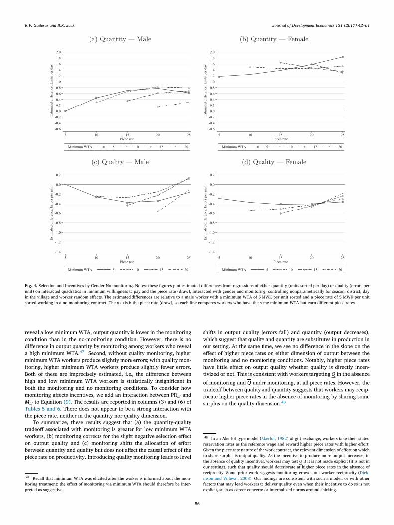
R.P. Guiteras and B.K. Jack Journal of Development Economics 131 (2017) 42–61

Fig. 4. Selection and Incentives by Gender No monitoring. Notes: these figures plot estimated differences from regressions of either quantity (units sorted per day) or quality (errors perunit) on interacted quadratics in minimum willingness to pay and the piece rate (draw), interacted with gender and monitoring, controlling nonparametrically for season, district, dayin the village and worker random effects. The estimated differences are relative to a male worker with a minimum WTA of 5 MWK per unit sorted and a piece rate of 5 MWK per unitsorted working in a no-monitoring contract. The x-axis is the piece rate (draw), so each line compares workers who have the same minimum WTA but earn different piece rates.

reveal a low minimum WTA, output quantity is lower in the monitoringcondition than in the no-monitoring condition. However, there is nodifference in output quantity by monitoring among workers who reveala high minimum WTA.47 Second, without quality monitoring, higherminimum WTA workers produce slightly more errors; with quality mon-itoring, higher minimum WTA workers produce slightly fewer errors.Both of these are imprecisely estimated, i.e., the difference betweenhigh and low minimum WTA workers is statistically insignificant inboth the monitoring and no monitoring conditions. To consider howmonitoring affects incentives, we add an interaction between PRid andMid to Equation (9). The results are reported in columns (3) and (6) ofTables 5 and 6. There does not appear to be a strong interaction withthe piece rate, neither in the quantity nor quality dimension.

To summarize, these results suggest that (a) the quantity-qualitytradeoff associated with monitoring is greater for low minimum WTAworkers, (b) monitoring corrects for the slight negative selection effecton output quality and (c) monitoring shifts the allocation of effortbetween quantity and quality but does not affect the causal effect of thepiece rate on productivity. Introducing quality monitoring leads to level

47 Recall that minimum WTA was elicited after the worker is informed about the mon-itoring treatment; the effect of monitoring via minimum WTA should therefore be inter-preted as suggestive.

shifts in output quality (errors fall) and quantity (output decreases),which suggest that quality and quantity are substitutes in production inour setting. At the same time, we see no difference in the slope on theeffect of higher piece rates on either dimension of output between themonitoring and no monitoring conditions. Notably, higher piece rateshave little effect on output quality whether quality is directly incen-tivized or not. This is consistent with workers targeting Q in the absenceof monitoring and Q under monitoring, at all piece rates. However, thetradeoff between quality and quantity suggests that workers may recip-rocate higher piece rates in the absence of monitoring by sharing somesurplus on the quality dimension.48

48 In an Akerlof-type model (Akerlof, 1982) of gift exchange, workers take their statedreservation rates as the reference wage and reward higher piece rates with higher effort.Given the piece rate nature of the work contract, the relevant dimension of effort on whichto share surplus is output quality. As the incentive to produce more output increases, inthe absence of quality incentives, workers may test Q if it is not made explicit (it is not inour setting), such that quality should deteriorate at higher piece rates in the absence ofreciprocity. Some prior work suggests monitoring crowds out worker reciprocity (Dick-inson and Villeval, 2008). Our findings are consistent with such a model, or with otherfactors that may lead workers to deliver quality even when their incentive to do so is notexplicit, such as career concerns or internalized norms around shirking.

56

R.P. Guiteras and B.K. Jack Journal of Development Economics 131 (2017) 42–61

Fig. 5. Selection and Incentives by Gender Monitoring. Notes: these figures plot estimated differences from regressions of either quantity (units sorted per day) or quality (errors perunit) on interacted quadratics in minimum willingness to pay and the piece rate (draw), interacted with gender and monitoring, controlling nonparametrically for season, district, dayin the village and worker random effects. The estimated differences are relative to a male worker with a minimum WTA of 5 MWK per unit sorted and a piece rate of 5 MWK per unitsorted working in a no-monitoring contract. The x-axis is the piece rate (draw), so each line compares workers who have the same minimum WTA but earn different piece rates.

4.3. Gender differences

To examine differential selection and effort choices by gender, werepeat the analyses and interact key regressors with a dummy variableindicating that the participant is female. Differences in reservation piecerates are obtained by re-estimating Equation (7) with interactions of thefemale variable with the labor season (High) and monitoring treatment(M). Table 7 shows the results for reservation rates by gender.49 Over-all, women are willing to work for less: their WTA is 2.3–3.0 Kwachalower than that of men. Quality monitoring has an imprecisely negativeeffect on minimum WTA for both men and women, with an insignifi-cantly larger effect for men. Women, but not men, display lower min-imum WTA in the high season (columns 1 and 3). The strength of thisrelationship is reduced for both women and men when including indi-vidual controls (columns 2 and 4), but much more so for women, bothin absolute and relative terms, suggesting strong selection for womenon covariates negatively associated with minimum WTA.

In discussing gender differences in productivity, as in Section 4.2,we begin with descriptive results from a flexible parametric specifica-tion, specifically by estimating a variant of Equation (9), but here inter-

49 Table S14 replicates the analysis of Table 7 but using interval regression as the esti-mator, with similar results.

acting the terms of interest with an indicator for whether the workeris female, instead of an indicator for the monitoring treatment. Specifi-cally, we estimate

yid = 𝛽1minWTAid + 𝛽2minWTA2id + 𝛽3PRid + 𝛽4PR2

id

+ 𝛽5(minWTAid × PRid

)+ 𝛽6

(Fid × minWTAid

)+ 𝛽7

(Fid × minWTA2

id)+ 𝛽8

(Fid × PRid

)+ 𝛽9

(Fid × PR2

id)+ 𝛽10

(Fid × minWTAid × PRid

)+ 𝜆Mid + 𝜙Highi + 𝜁Fi + 𝜏DoWd + 𝛿Disti + ci + 𝜀id, (10)

with worker random effects and calculate estimated differences relativeto the omitted category of a worker in the no monitoring treatment,with a minimum WTA of 5 MWK per unit sorted, and facing a piece rateof 5 MWK. These estimates, plotted in Fig. 3, shows that male workersare more heterogeneous, and that the negative selection effect notedabove is largely concentrated among men. This interpretation becomeseven more clear when we further interact with monitoring, as in Figs. 4and 5 – women are somewhat less heterogeneous than men withoutmonitoring (Fig. 4), and monitoring largely eliminates heterogeneityamong women, but not men (Fig. 5).

Differences in productivity, controlling for reservation piece rates,are obtained by re-estimating Equation (9) allowing the effects of mon-

57

R.P. Guiteras and B.K. Jack Journal of Development Economics 131 (2017) 42–61

Table 8Determinants of quantity (number of units sorted per day) differential effects by gender.

Pooled OLS Random Effects

(1) (2) (3) (4) (5) (6)

MonitoringAmong Men −0.383***

(0.143)−0.360(0.295)

0.252(0.421)

−0.376***

(0.115)−0.196(0.233)

−0.127(0.343)

Among Women −0.662***

(0.098)−0.792***

(0.206)−0.729**

(0.285)−0.654***

(0.075)−0.811***

(0.167)−0.901***

(0.239)

Minimum WTAAmong Men −0.023

(0.018)−0.022(0.023)

−0.024(0.018)

−0.048***

(0.018)−0.039**

(0.019)−0.049***

(0.018)Among Women 0.005

(0.014)−0.002(0.019)

0.005(0.014)

−0.009(0.012)

−0.019(0.015)

−0.009(0.012)

Monitoring X Minimum WTAAmong Men −0.002

(0.029)−0.019(0.023)

Among Women 0.015(0.021)

0.019(0.017)

Piece rateAmong Men 0.014

(0.011)0.014(0.011)

0.035**

(0.018)0.027***

(0.010)0.026***

(0.010)0.035***

(0.013)Among Women 0.020***

(0.008)0.020***

(0.008)0.018(0.011)

0.026***

(0.006)0.026***

(0.006)0.019**

(0.008)

Monitoring X Piece rateAmong Men −0.036*

(0.022)−0.014(0.017)

Among Women 0.004(0.015)

0.014(0.013)

High SeasonAmong Men 0.905***

(0.212)0.904***

(0.213)0.887***

(0.213)0.962***

(0.209)0.956***

(0.210)0.956***

(0.210)Among Women 0.313*

(0.160)0.311*

(0.159)0.309*

(0.160)0.260*

(0.154)0.260*

(0.154)0.253(0.155)

Female Level Effect 0.923**

(0.367)0.997**

(0.396)1.304***

(0.456)0.985***

(0.318)1.142***

(0.331)1.241***

(0.379)Mean Dep. Var. 7.350 7.350 7.350 7.350 7.350 7.350SD Dep. Var. 1.975 1.975 1.975 1.975 1.975 1.975Num. of participants 612 612 612 612 612 612Num. of observations 1461 1461 1461 1461 1461 1461

Notes: this table presents differential effects by gender of whether the participant was assigned to the monitoring treatment,the minimum piece rate the participant was willing to accept (Minimum WTA), the piece rate the participant received (PieceRate), and season on quantity (number of units sorted per day). Columns (2) and (5) interact minimum WTA with monitoring;columns (3) and (6) interact the piece rate with monitoring. Columns (1)–(3) are estimated by pooled OLS, columns (4)–(6)with worker random effects. All regressions include controls for individual covariates as in Table 6, day-of-week fixed effects,and district fixed effects. Standard errors robust to clustering at the worker level in parentheses * p < 0.10, ** p < 0.05, ***

p < 0.01.

itoring, minimum WTA, the piece rate and the labor season to vary bygender. Tables 8 and 9 show the effects on the quantity of output andquality of output respectively.

Recall that, on average, females sort more units of beans with fewererrors than do men. Monitoring reduces the quantity of output for bothgenders, but more so for females (Table 8). The pure incentive effectof the piece rate on quantity of output is similar across genders. How-ever, the selection effect of minimum WTA on quantity of output doesvary by gender. Men who exhibit a higher minimum WTA rate sortfewer units of beans (a 10 MWK increase in the reservation piece rate isassociated with sorting 1/5 to 1/2 fewer units per day, significant onlyin the random effects specifications); among women, the relationshipis inconsistently signed and insignificant. Thus, the negative selectiondescribed in Section 4.2 is driven entirely by the men in the sample.This is plausible if women’s outside options are more similar to beansorting, while men’s outside options depend more on physical capacity,as in the returns to brawn in Pitt et al. (2012), or if men who producehigher output also have a lower minimum willingness to accept, consis-tent with cash needs driving both margins.

Survey evidence helps address alternative interpretations of the neg-ative selection observed among men. First, expected output is positivelycorrelated with actual output for both men and women, indicating thatmen are not systematically more likely to mis-estimate their own pro-ductivity. In fact, men on average make more accurate predictions oftheir output. Second, reporting a cash-generating outside option is neg-atively correlated with reservation piece rates, even within participant.Men are significantly more likely to report an outside option that gener-ates cash earnings, such as other casual labor, while women are signif-icantly more likely to report housework as their outside option. Third,high productivity men who state low reservation rates are not able tomake up for lower piece rates with higher output: for a given piecerate, daily earnings do not increase with minimum WTA. Factors notmeasured in our survey may also matter. If, for example, women placeextra value on the earnings in the experiment because they can be keptprivate, then they may both be willing to work for less and may workharder conditional on receiving a contract, consistent with the genderdifferences we observe.

58

R.P. Guiteras and B.K. Jack Journal of Development Economics 131 (2017) 42–61

Table 9Determinants of quality (number of errors per unit sorted) differential effects by gender.

Pooled OLS Random Effects

(1) (2) (3) (4) (5) (6)

MonitoringAmong Men −0.648***

(0.094)−0.446**

(0.195)−0.672**

(0.323)−0.589***

(0.091)−0.402**

(0.189)−0.761**

(0.300)Among Women −0.653***

(0.050)−0.628***

(0.109)−0.725***

(0.156)−0.631***

(0.047)−0.627***

(0.105)−0.674***

(0.150)

Minimum WTAAmong Men −0.008

(0.011)0.002(0.017)

−0.008(0.011)

−0.006(0.011)

0.004(0.016)

−0.006(0.011)

Among Women −0.003(0.007)

−0.001(0.009)

−0.003(0.007)

−0.002(0.007)

−0.002(0.009)

−0.002(0.007)

Monitoring X Minimum WTAAmong Men −0.021

(0.019)−0.020(0.018)

Among Women −0.003(0.011)

−0.000(0.011)

Piece rateAmong Men 0.022**

(0.009)0.022**

(0.009)0.022(0.014)

0.021**

(0.009)0.021**

(0.009)0.015(0.014)

Among Women 0.004(0.004)

0.004(0.004)

0.002(0.007)

0.005(0.004)

0.005(0.004)

0.003(0.007)

Monitoring X Piece rateAmong Men 0.001

(0.018)0.010(0.017)

Among Women 0.004(0.009)

0.003(0.008)

High SeasonAmong Men −0.199

(0.126)−0.205(0.125)

−0.198(0.125)

−0.199(0.129)

−0.205(0.128)

−0.195(0.128)

Among Women 0.036(0.065)

0.038(0.065)

0.034(0.065)

0.021(0.068)

0.023(0.068)

0.020(0.069)

Female Level Effect −0.107(0.208)

−0.021(0.248)

−0.085(0.320)

−0.101(0.205)

−0.015(0.240)

−0.173(0.301)

Mean Dep. Var. 1.883 1.883 1.883 1.883 1.883 1.883SD Dep. Var. 1.013 1.013 1.013 1.013 1.013 1.013Num. of participants 612 612 612 612 612 612Num. of observations 1461 1461 1461 1461 1461 1461

Notes: this table presents differential effects by gender of whether the participant was assigned to the monitoring treatment,the minimum piece rate the participant was willing to accept (Minimum WTA), the piece rate the participant received (PieceRate), and season on quality (number of errors per unit sorted). Columns (2) and (5) interact minimum WTA with monitoring;columns (3) and (6) interact the piece rate with monitoring. Columns (1)–(3) are estimated by pooled OLS, columns (4)–(6)with worker random effects. All regressions include controls for individual covariates as in Table 6, day-of-week fixed effects,and district fixed effects. Standard errors robust to clustering at the worker level in parentheses * p < 0.10, ** p < 0.05, ***

p < 0.01.

In spite of the differences in minimum WTA across season amongwomen, output by women is the same in the high and low season. Men,on the other hand, produce more output in the high season than in thelow season, approximately one unit per day. This difference may also berelated to the differences in men and women’s outside options and needfor cash income, and how they vary with the labor season, or to differ-ences in the subject pool in the low and high labor demand seasons.

Both men and women are similarly responsive to monitoring in theirallocation of effort toward output quality (Table 9, with additionalresults in Tables S15 and S16). The piece rate has a small positive effecton the error rate for men and no effect for women. Minimum WTA isnot associated with the error rate for either men or for women. Men do,however, reduce the number of errors per unit sorted in the high season,while error rates for women do not differ significantly across seasons.

5. Discussion

We implement a unique experimental design in casual labor mar-kets in rural Malawi to understand the workings of a common form of

piece-rate labor, to observe gender differences in these markets and totest for other behavioral determinants of productivity. Raising the piecerate has little effect on the quality of worker interested in the job; if any-thing, selection effects are associated with lower productivity. On theother hand, a higher piece rate significantly increases the quantity ofoutput, controlling for workers’ reservation rates, but does not reducequality. Explicit incentives for output quality reduce the error rate inproduction at some cost to output quantity, but do not affect workerwillingness to accept the task. Furthermore, the more complete con-tracts that include quality incentives appear to regularize output andreduce some of the differences in response to the piece rate that arisethrough worker self-selection when quality is unmonitored.

Comparing the extensive (participation) versus intensive (effort)margins, conditional on showing up to the experiment, participation ismore responsive to the piece rate than is effort. Over the range of piecerates offered, the arc elasticity of participation with respect to the piecerate is 0.58 (Table S17), while the elasticity of output quantity withrespect to the piece rate (controlling for the reservation piece rate) is0.06 (Table S18). The reasonably high participation elasticity suggests

59

R.P. Guiteras and B.K. Jack Journal of Development Economics 131 (2017) 42–61

that the variation in piece rates in our study has a substantial effecton hiring outcomes, conditional on showing up for the experiment. SeeTables S17 and S18 for details. At the mean, introducing monitoringlowers output as much as a 30 MWK decrease in the piece rate. It takesworkers in the monitoring treatment about 0.7 days longer to sort a50 kg bag of beans than workers who are not being monitored. Well-sorted beans sell for up to 4000 MWK more per 50 kg bag than unsortedbeans, potentially justifying the time cost of monitoring.

We perform a simple calibration of employer profits at differentpiece rates, with and without quality monitoring, and by gender. (SeeSection S3 of the Supplementary Materials for details.) Assuming apenalty for mis-sorted beans, and costs per worker-day associated withhiring and administering the work and with quality monitoring, theemployer prefers to monitor output quality at all piece rates. Under ourmain assumptions about the quality premium and supervision costs, thehighest overall profit per bag comes from the lowest piece rate com-bined with worker penalties for low quality output, i.e., the contractthat is least profitable to the worker. However, the profit-maximizingcontract depends on the gender of the worker. The profit implicationsof quality monitoring are modest when the worker is female, and theprofit-maximizing contract for a female worker is a low piece rate with-out monitoring. For male workers, on the other hand, profits vary con-siderably more with the contractual arrangements: at low piece rates,profits are nearly 50 percent higher if quality is monitored, makinglow piece rates with quality monitoring the contract that maximizesthe employer’s profit when hiring a male worker. Higher piece ratesnarrow the profitability gap between monitored and unmonitored maleworkers. Differences in the profit-maximizing contract by gender ariseexclusively from the worker responses that we document, and giveemployers an incentive to discriminate based on this easily observedtrait. Overall, the high acceptance rates for the contractual arrange-ments that are least favorable to the worker, together with selectioneffects from higher piece rates that are, if anything, negative in thesample that shows up to our experiment, make high piece rates evenless attractive from the perspective of the employer. In our study set-ting, rural households have few well-paying outside options for cashearnings, which places the bargaining power squarely in the hands ofthe employer.

The context in which the study takes place appears to shape manyof the findings. For example, qualitative survey evidence (see Section3.2) suggests that quality monitoring is common in piece rate workarrangements, and accompanied by high penalties for violation of onlyloosely defined quality standards. Participants in our study may havetherefore preferred the more complete terms offered by the monitoringcontract over the potentially ambiguous contract without explicit qual-ity monitoring. As another example, men and women in our setting facedifferent outside options, which are more likely to involve hard man-ual labor for men and tasks like weeding or home activities for women,similar to the setting of Pitt et al. (2012). This may explain some of theobserved negative selection by men in our study. The available outsideoptions also vary across the high and low labor demand seasons as doliquidity constraints. When the value of money is high, during the highlabor demand season, workers have a lower WTA and are more respon-sive to incentives. We also observe that minimum WTA is lower amongparticipants who report an outside option associated with other income-generating activities, including those that would help meet immediatecash needs, such as other casual labor (see Table S7).50

Our study is limited in its ability to draw strong conclusions aboutthe role of outside markets in shaping behavior within the experiment.Future work that generates exogenous variation in the value of the out-side option would offer a more direct test of the hypothesis that labor

50 This is also consistent with Goldberg (2016), who reports that 70 percent of partic-ipants in her study report immediate cash needs as their reason for working. Fink et al.(2014) provide further evidence from a similar setting in neighboring Zambia that cashneeds drive casual labor supply, particularly during the high season.

market imperfections undermine sorting of workers based on productiv-ity. In addition, additional data collection that offers a more nuancedpicture of the contractual forms common for different tasks and in dif-ferent markets would facilitate further study of the contracting frictionsin rural labor markets. Finally, our results suggest that further data col-lection on the prevalence of piece rate contracts in developing countryrural wages would stimulate additional research into the structure anddistributional effects of rural labor markets, between men and women,and between employers and workers.

Appendix A. Supplementary data

Supplementary data related to this article can be found at https://doi.org/10.1016/j.jdeveco.2017.11.002.

References

Akerlof, George A., 1982. Labor contracts as partial gift exchange. Q. J. Econ. 97 (4),543–569.

Ashraf, Nava, Berry, James, Shapiro, Jesse M., 2010. Can higher prices stimulateproduct use? Evidence from a field experiment in Zambia. Am. Econ. Rev. 100 (5),2383–2413.

Atkin, David, Chaudhry, Azam, Chaudry, Shamyla, Khandelwal, Amit K., Verhoogen,Eric, 2017. Organizational barriers to technology adoption: evidence fromsoccer-ball producers in Pakistan. Q. J. Econ. 132 (3), 1101–1164.

Baker, George P., 1992. Incentive contracts and performance measurement. J. PoliticalEcon. 100 (3), 598–614.

Baland, Jean-Marie, Drèze, Jean, Leruth, Luc, 1999. Daily wages and piece rates inagrarian economies. J. Dev. Econ. 59 (2), 445–461.

Bandiera, Oriana, Barankay, Iwan, Rasul, Imran, 2005. Social preferences and theresponse to incentives: evidence from personnel data. Q. J. Econ. 120 (3), 917–962.

Bandiera, Oriana, Barankay, Iwan, Rasul, Imran, 2010. Social incentives in theworkplace. Rev. Econ. Stud. 77 (2), 417–458.

Bandiera, Oriana, Fischer, Greg, Prat, Andrea, Ytsma, Erina, 2016. Do Women RespondLess to Performance Pay? Building Evidence from Multiple Experiments. Mimeo.

Bardhan, Pranab K., 1979. Labor supply functions in a poor agrarian economy. Am.Econ. Rev. 69 (1), 73–83.

Beaman, Lori, Keleher, Niall, Magruder, Jeremy, 2015. Do Job Networks DisadvantageWomen? Evidence from a Recruitment Experiment in Malawi. Mimeo.

Becker, G., DeGroot, M., Marschak, J., 1964. Measuring utility by a single-responsesequential method. Behav. Sci. 9, 226–236.

Behrman, Jere R., 1999. Labor markets in developing countries. In: Handbook of LaborEconomics, Volume 3, Part B. Elsevier, pp. 2859–2939.

Berry, James, Fischer, Greg, Guiteras, Raymond, 2015. Eliciting and UtilizingWillingness to Pay: Evidence from Field Trials in Northern Ghana. Mimeo.

Chang, Tom, Gross, Tal, 2014. How many pears would a pear packer pack if a pearpacker could pack pears at quasi-exogenously varying piece rates? J. Econ. Behav.Organ. 99, 1–17.

Chassang, Sylvain, Padro i Miquel, Gerard, Snowberg, Erik, 2012. Selective trials: aprincipal-agent approach to randomized controlled experiments. Am. Econ. Rev.102 (4), 1279–1309.

Cohen, Jessica, Dupas, Pascaline, 2010. Free distribution or cost-sharing? Evidence froma randomized malaria prevention experiment. Q. J. Econ. 125 (1), 1–45.

Dickinson, David, Villeval, Marie-Claire, 2008. Does monitoring decrease work effort?:the complementarity between agency and crowding-out theories. Games Econ.Behav. 63 (1), 56–76.

Dimowa, Ralitza, Michaelowa, Katharina, Weber, Anke, 2010. Ganyu labour in Malawi:understanding rural households’ labour supply strategies. In: Number 29 inProceedings of the German Development Economics Conference.

Dohmen, Thomas, Falk, Armin, 2011. Performance pay and multidimensional sorting:productivity, preferences, and gender. Am. Econ. Rev. 101 (2), 556–590.

Dupas, P., Robinson, J., 2013. The Daily Grind: Cash Needs, Labor Supply andSelf-control. Mimeo.

Eriksson, Tor, Villeval, Marie Claire, 2008. Performance-pay, sorting and socialmotivation. J. Econ. Behav. Organ. 68 (2), 412–421.

Eswaran, Mukesh, Kotwal, Ashok, 1985. A theory of contractual structure in agriculture.Am. Econ. Rev. 75 (3), 352–367.

Farber, Henry S., 2005. Is tomorrow another day? The labor supply of New York Citycabdrivers. J. Political Econ. 113 (1), 46–82.

Fehr, Ernst, Goette, Lorenz, 2007. Do workers work more if wages are high? Evidencefrom a randomized field experiment. Am. Econ. Rev. 97 (1), 298–317.

Fink, Günther, Kelsey Jack, B., Masiye, Felix, 2014. Seasonal Credit Constraints andAgricultural Labor supply: Evidence from Zambia. Mimeo.

Foster, Andrew D., Rosenzweig, Mark R., 1994. A test for moral hazard in the labormarket: contractual arrangements, effort, and health. Rev. Econ. Statistics 72 (2),213–227.

Foster, Andrew D., Rosenzweig, Mark R., 1996. Comparative advantage, informationand the allocation of workers to tasks: evidence from an agricultural labour market.Rev. Econ. Stud. 63 (3), 347–374.

Goldberg, Jessica, 2016. Kwacha gonna do? Experimental evidence about labor supplyin rural Malawi. Am. Econ. J. Appl. Econ. 8 (1), 129–149.

60

R.P. Guiteras and B.K. Jack Journal of Development Economics 131 (2017) 42–61

Hamilton, Barton H., Nickerson, Jack A., Owan, Hideo, 2003. Team incentives andworker heterogeneity: an empirical analysis of the impact of teams on productivityand participation. J. Political Econ. 111 (3), 465–497.

Heywood, J., Siebert, S., Wei, X., 2013. The Consequences of a Piece Rate on Quantityand Quality: Evidence from a Field Experiment. Mimeo.

Hoffman, Vivian, 2009. Intrahousehold allocation of free and purchased mosquito nets.Am. Econ. Rev. 99 (2), 236–241.

Jayaraman, Rajshri, Lanjouw, Peter, 1999. The evolution of poverty and inequality inIndian villages. World Bank Res. Obs. 14 (1), 1–30.

Karlan, Dean, Zinman, Jonathan, 2009. Observing unobservables: identifyinginformation asymmetries with a consumer credit field experiment. Econometrica 77(6), 1993–2008.

Kim, Hyuncheol Bryant, Kim, Seonghoon, T. Kim, Thomas, 2017. The selection andcausal effects of work incentives on labor productivity: evidence from a two-stagerandomized controlled trial in Malawi. Mimeo.

Lazear, Edward P., 2000. Performance pay and productivity. Am. Econ. Rev. 90 (5),1346–1361.

Nagin, Daniel S., Rebitzer, James B., Sanders, Seth, Taylor, Lowell J., 2002. Monitoring,motivation, and management: the determinants of opportunistic behavior in a fieldexperiment. Am. Econ. Rev. 92 (4), 850–873.

Newman, Constance, Jarvis, Lovell, 2000. Worker and firm determinants of piece ratevariation in an agricultural labor market. Econ. Dev. Cult. Change 49 (1), 137–169.

Ortiz, Sutti, October 2002. Laboring in the factories and in the fields. Annu. Rev.Anthropol. 31 (1), 395–417.

Paarsch, Harry J., Shearer, Bruce S., 1999. The response of worker effort to piece rates:evidence from the British Columbia tree-planting industry. J. Hum. Resour. 34 (4),643–667.

Pitt, Mark M., Rosenzweig, Mark R., Hassan, Mohammad Nazmul, 2012. Human capitalinvestment and the gender division of labor in a brawn-based economy. Am. Econ.Rev. 102 (7), 3531–3560.

Rosenzweig, Mark R., 1978. Rural wages, labor supply, and land reform: a theoreticaland empirical analysis. Am. Econ. Rev. 68 (5), 847–861.

Rosenzweig, Mark R., 1988. Chapter Labor Markets in Low-income Countries. Handbookof Development Economics, vol. 1. Elsevier, pp. 713–762.

Roumasset, James, Lee, Sang-Hyop, 2007. Chapter Labor: Decisions, Contracts andOrganization. Handbook of Agricultural Economics, vol. 3. Elsevier, pp. 2705–2740.

Schoar, Antoinette, 2014. The Importance of Being Nice: Supervisory Skill Training inthe Cambodian Garment Industry. Mimeo.

Sitienei, Isaac, Mishra, Ashok K., Khanal, Aditya R., 2016. Informal Ganyu Labor Supply,and Food Security: the Case of Malawi, Chapter 11, pp. 159–175.

Stiglitz, Joseph E., 1975. Incentives, risk, and information: notes towards a theory ofhierarchy. Bell J. Econ. 6 (2), 552–579.

Whiteside, Martin, 2000. Ganyu Labor in Malawi and its Implications for LivelihoodSecurity Interventions. Mimeo.

61