Prof. Bodik CS 164 Lecture 16, Fall 20041 Global Optimization Lecture 16

Prof. Bodik CS 164 Lecture 16, Fall 2004 1

Global Optimization

Lecture 16

Prof. Bodik CS 164 Lecture 16, Fall 2004

2

Lecture Outline

• Global flow analysis

• Global constant propagation

• Liveness analysis


3

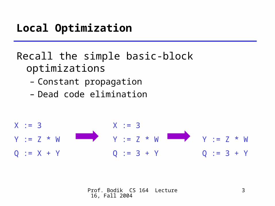
Local Optimization

Recall the simple basic-block optimizations– Constant propagation– Dead code elimination

X := 3

Y := Z * W

Q := X + Y

X := 3

Y := Z * W

Q := 3 + Y

Y := Z * W

Q := 3 + Y


4

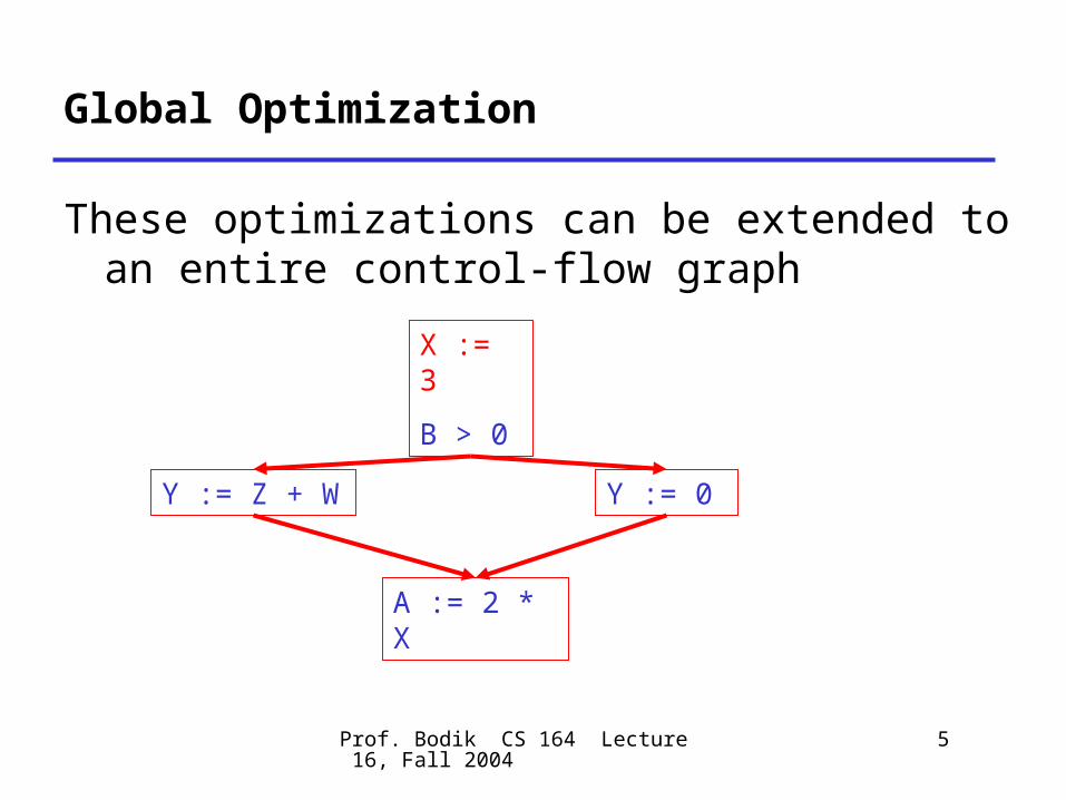
Global Optimization

These optimizations can be extended to an entire control-flow graph

X := 3

B > 0

Y := Z + W Y := 0

A := 2 * X


5

Global Optimization


X := 3

B > 0

Y := Z + W Y := 0

A := 2 * X


6

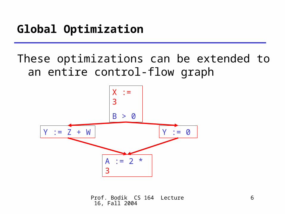
Global Optimization


X := 3

B > 0

Y := Z + W Y := 0

A := 2 * 3


7

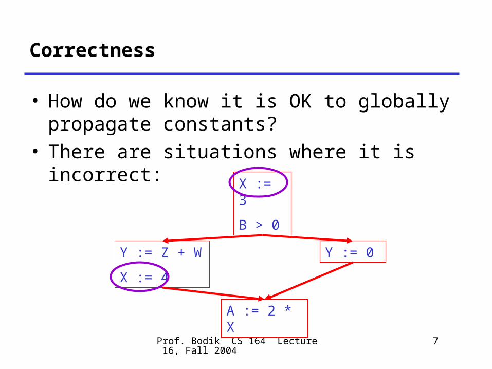
Correctness

• How do we know it is OK to globally propagate constants?

• There are situations where it is incorrect:

X := 3

B > 0

Y := Z + W

X := 4

Y := 0

A := 2 * X


8

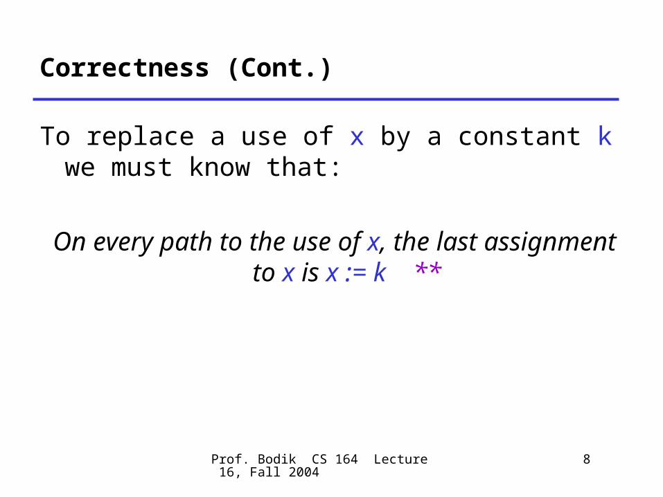
Correctness (Cont.)

To replace a use of x by a constant k we must know that:

On every path to the use of x, the last assignment to x is x := k **


9

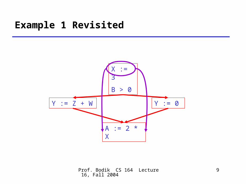
Example 1 Revisited

X := 3

B > 0

Y := Z + W Y := 0

A := 2 * X


10

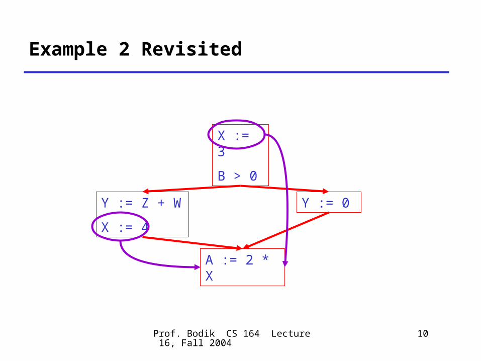
Example 2 Revisited

X := 3

B > 0

Y := Z + W

X := 4

Y := 0

A := 2 * X


11

Discussion

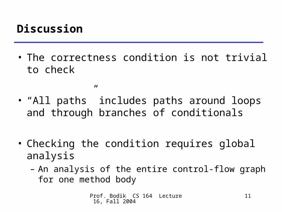
• The correctness condition is not trivial to check

• “All paths” includes paths around loops and through branches of conditionals

• Checking the condition requires global analysis– An analysis of the entire control-flow graph for

one method body


12

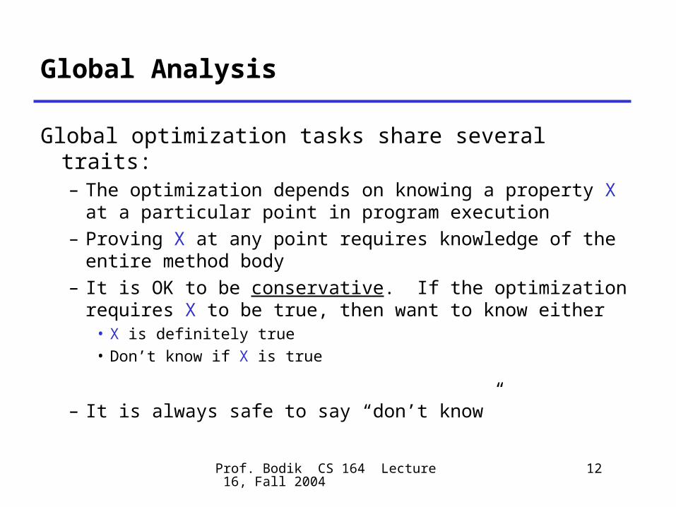
Global Analysis

Global optimization tasks share several traits:– The optimization depends on knowing a property

X at a particular point in program execution– Proving X at any point requires knowledge of the

entire method body– It is OK to be conservative. If the optimization

requires X to be true, then want to know either• X is definitely true• Don’t know if X is true

– It is always safe to say “don’t know”


13

Global Analysis (Cont.)

• Global dataflow analysis is a standard technique for solving problems with these characteristics

• Global constant propagation is one example of an optimization that requires global dataflow analysis


14

Global Constant Propagation

• Global constant propagation can be performed at any point where ** holds

• Consider the case of computing ** for a single variable X at all program points


15

Global Constant Propagation (Cont.)

• To make the problem precise, we associate one of the following values with X at every program point

value interpretation

This statement is not reachable

c X = constant c

* Don’t know if X is a constant


16

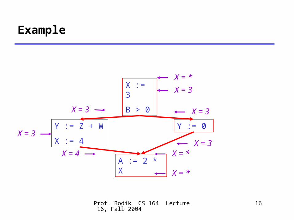
Example

X = *X = 3

X = 3

X = 3X =

4X = *

X := 3

B > 0

Y := Z + W

X := 4

Y := 0

A := 2 * X

X = 3

X = 3

X = *


17

Using the Information

• Given global constant information, it is easy to perform the optimization– Simply inspect the x = ? associated with a

statement using x– If x is constant at that point replace that use of

x by the constant

• But how do we compute the properties x = ?


18

The Idea

The analysis of a complicated program can be expressed as a combination of simple rules relating the change in information

between adjacent statements


19

Explanation

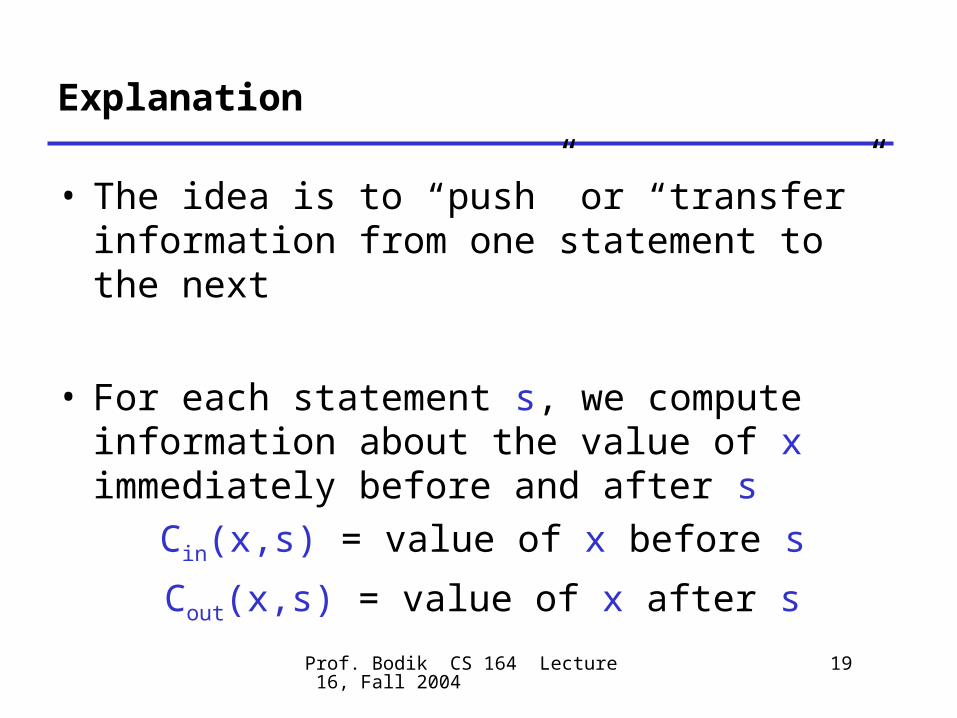
• The idea is to “push” or “transfer” information from one statement to the next

• For each statement s, we compute information about the value of x immediately before and after s

Cin(x,s) = value of x before s

Cout(x,s) = value of x after s


20

Transfer Functions

• Define a transfer function that transfers information from one statement to another

• In the following rules, let statement s have immediate predecessor statements p1,…,pn


21

Rule 1

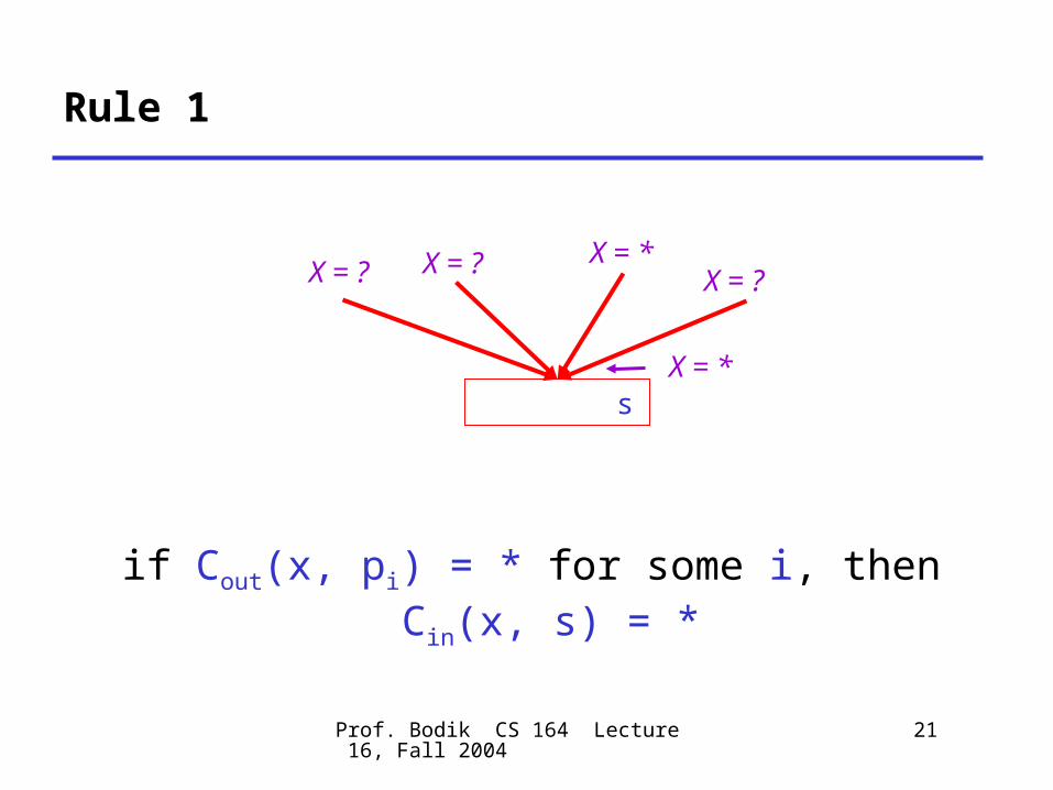
if Cout(x, pi) = * for some i, then Cin(x, s) = *

s

X = *

X = *

X = ?

X = ?

X = ?


22

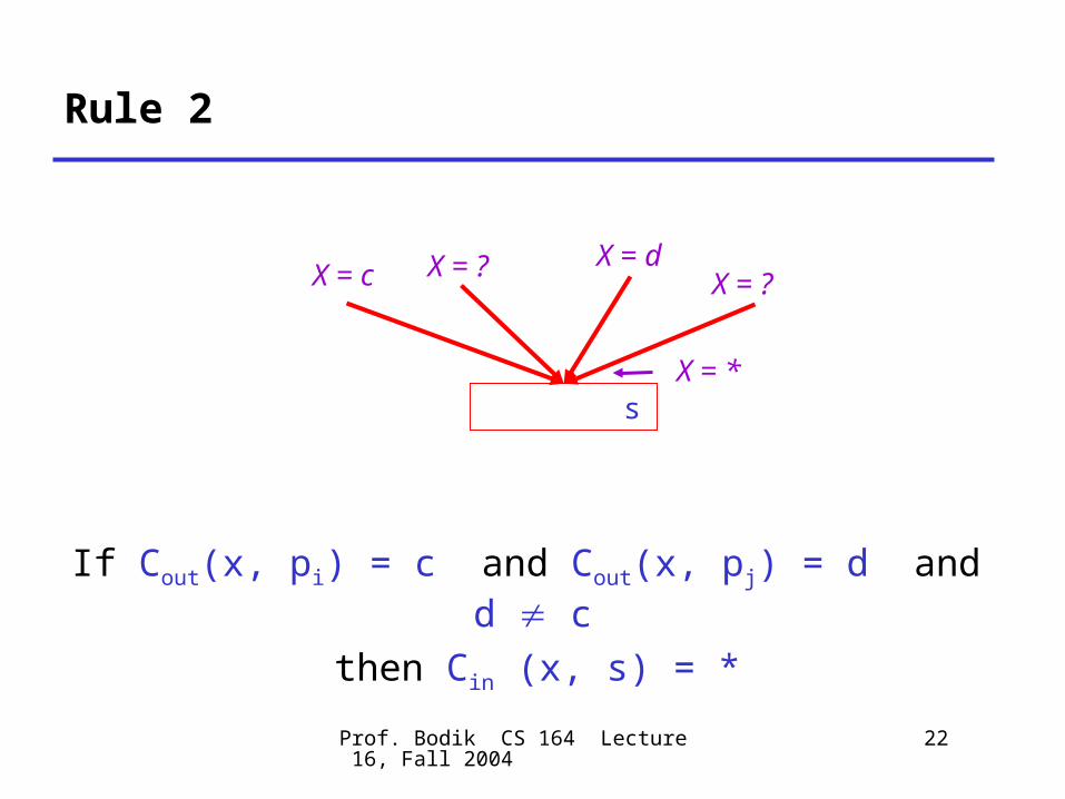
Rule 2

If Cout(x, pi) = c and Cout(x, pj) = d and d c

then Cin (x, s) = *

s

X = d

X = *

X = ?

X = ?

X = c


23

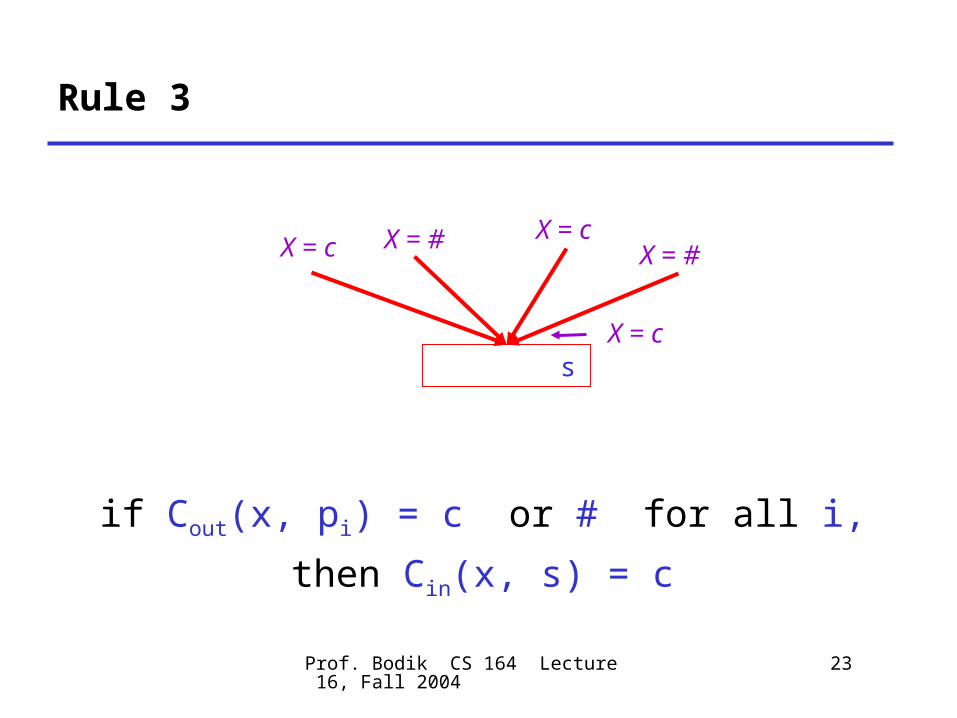
Rule 3

if Cout(x, pi) = c or # for all i,

then Cin(x, s) = c

s

X = c

X = c

X = #X = # X =

c


24

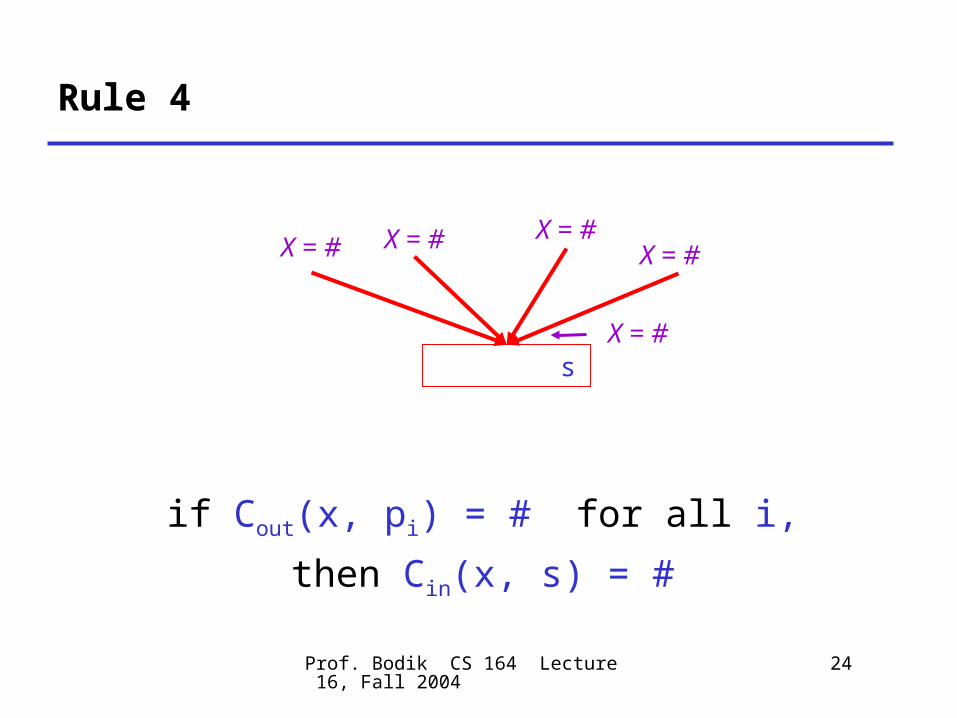
Rule 4

if Cout(x, pi) = # for all i,

then Cin(x, s) = #

s

X = #

X = #

X = #X = # X = #


25

The Other Half

• Rules 1-4 relate the out of one statement to the in of the successor statement– they propagate information forward across CFG

edges

• Now we need rules relating the in of a statement to the out of the same statement– to propagate information across statements


26

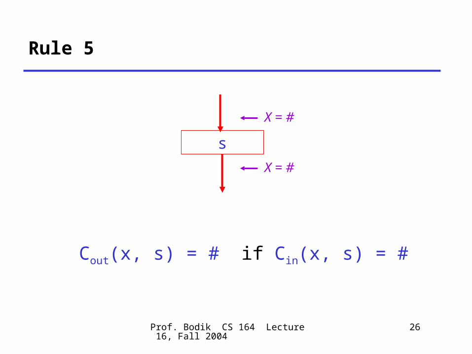
Rule 5

Cout(x, s) = # if Cin(x, s) = #

s

X = #

X = #


27

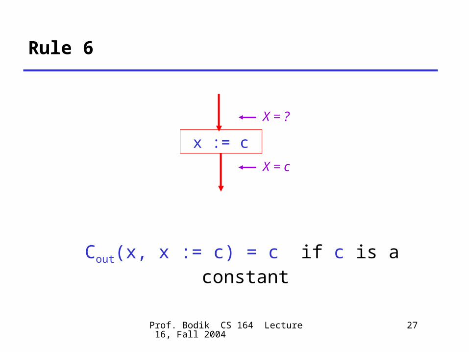
Rule 6

Cout(x, x := c) = c if c is a constant

x := c

X = ?

X = c


28

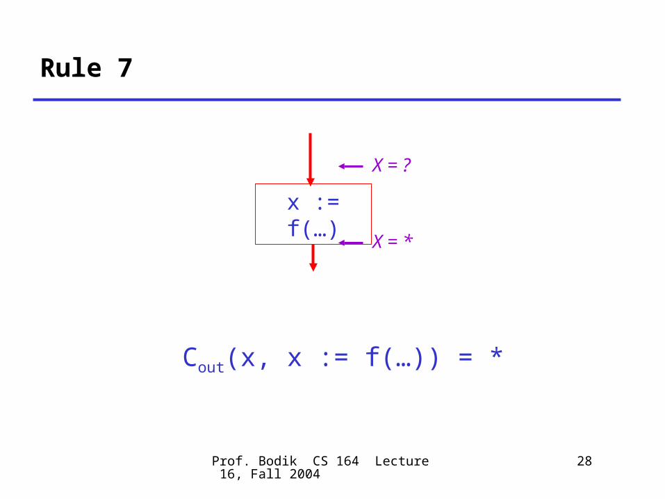
Rule 7

Cout(x, x := f(…)) = *

x := f(…)

X = ?

X = *


29

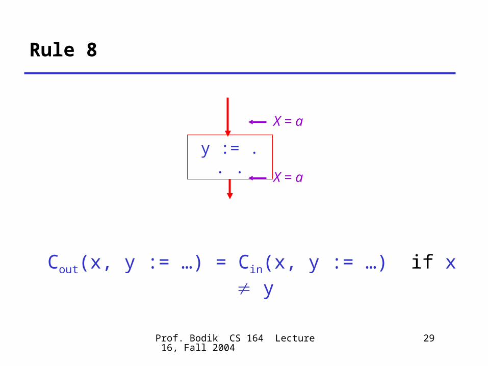
Rule 8

Cout(x, y := …) = Cin(x, y := …) if x y

y := . . .

X = a

X = a


30

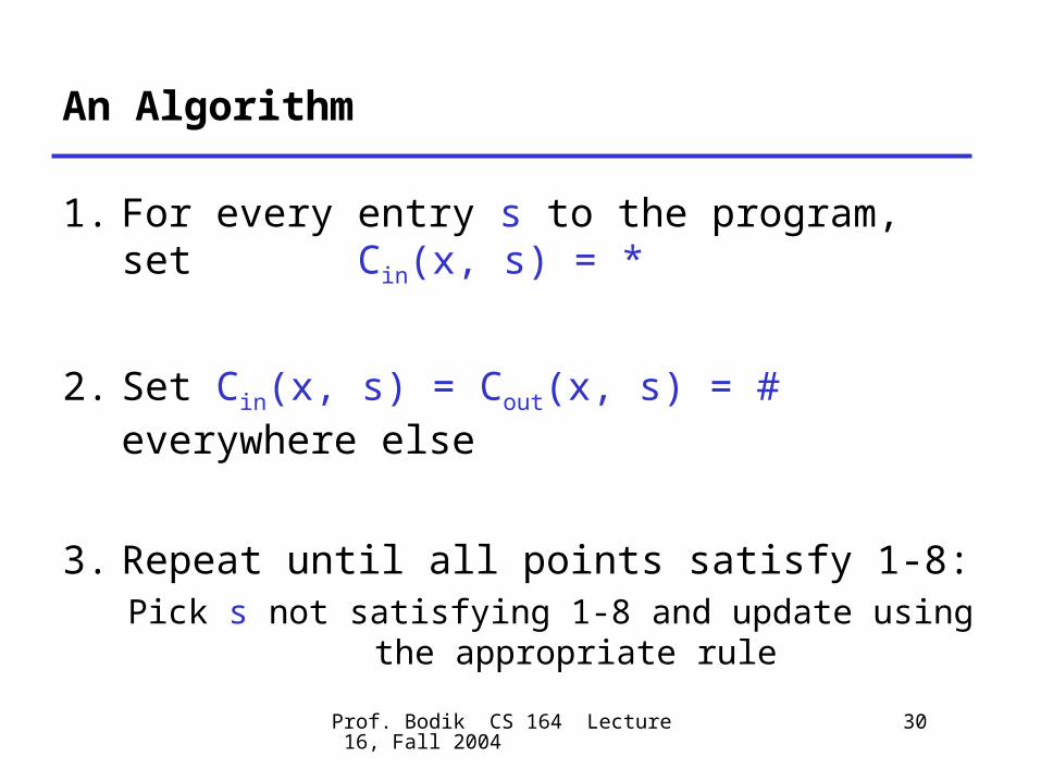
An Algorithm

1. For every entry s to the program, set Cin(x, s) = *

2. Set Cin(x, s) = Cout(x, s) = # everywhere else

3. Repeat until all points satisfy 1-8:Pick s not satisfying 1-8 and update using the

appropriate rule


31

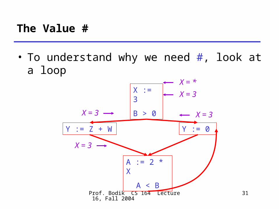
The Value #

• To understand why we need #, look at a loop

X := 3

B > 0

Y := Z + W Y := 0

A := 2 * X

A < B

X = *X = 3

X = 3

X = 3

X = 3


32

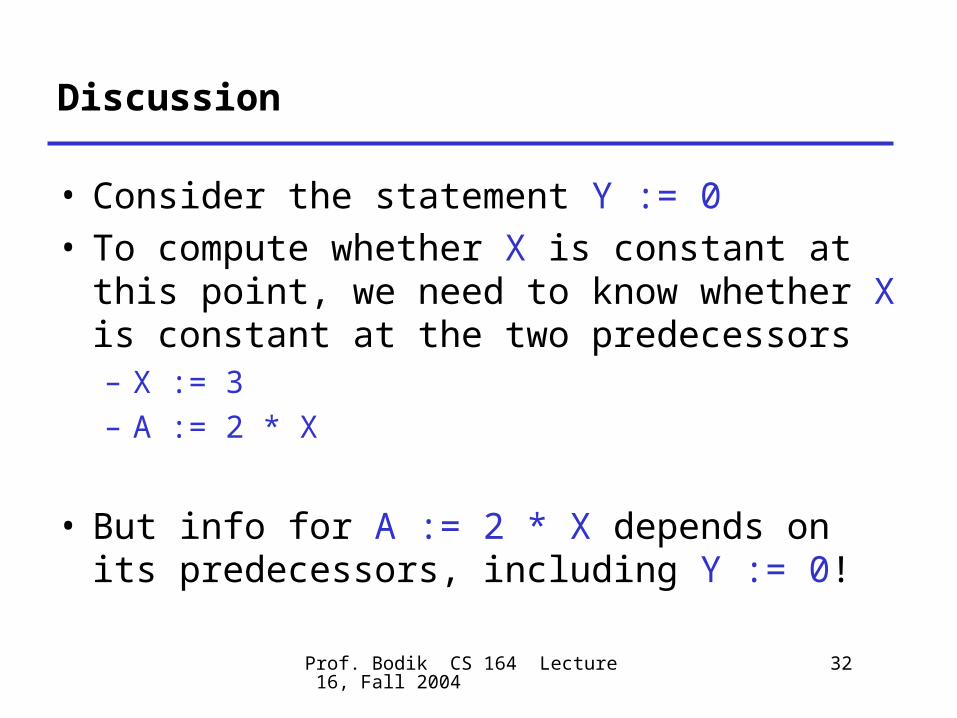
Discussion

• Consider the statement Y := 0• To compute whether X is constant at this

point, we need to know whether X is constant at the two predecessors– X := 3– A := 2 * X

• But info for A := 2 * X depends on its predecessors, including Y := 0!


33

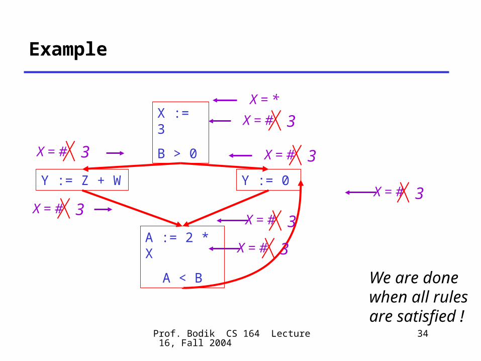
The Value # (Cont.)

• Because of cycles, all points must have values at all times

• Intuitively, assigning some initial value allows the analysis to break cycles

• The initial value # means “So far as we know, control never reaches this point”


34

Example

X := 3

B > 0

Y := Z + W Y := 0

A := 2 * X

A < B

X = *

X = #

X = #

X = #

X = #

X = #

X = #

X = #

3

3

3

3

3

3

3

We are donewhen all rulesare satisfied !


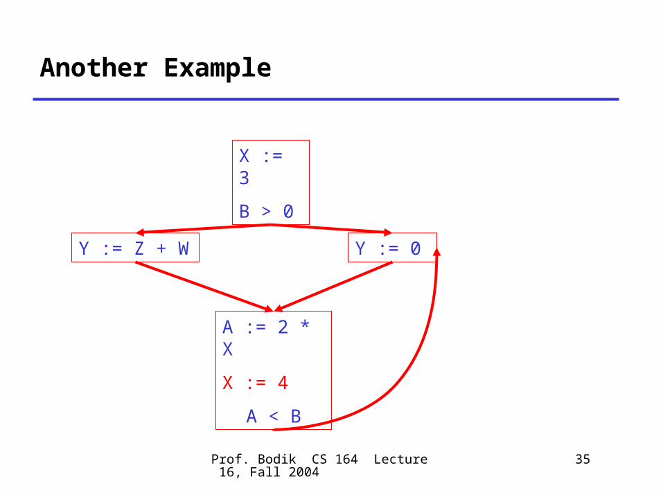
35

Another Example

X := 3

B > 0

Y := Z + W Y := 0

A := 2 * X

X := 4

A < B


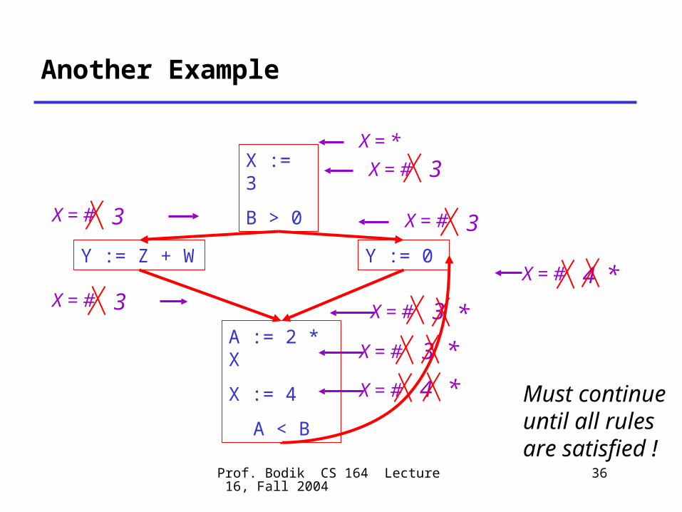
36

Another Example

X := 3

B > 0

Y := Z + W Y := 0

A := 2 * X

X := 4

A < B

X = *X = #

X = #

X = #

X = #

X = #

X = #

X = #

X = #

3

3

3

3

3

3

4

4

*

*

*

*

Must continue until all rulesare satisfied !


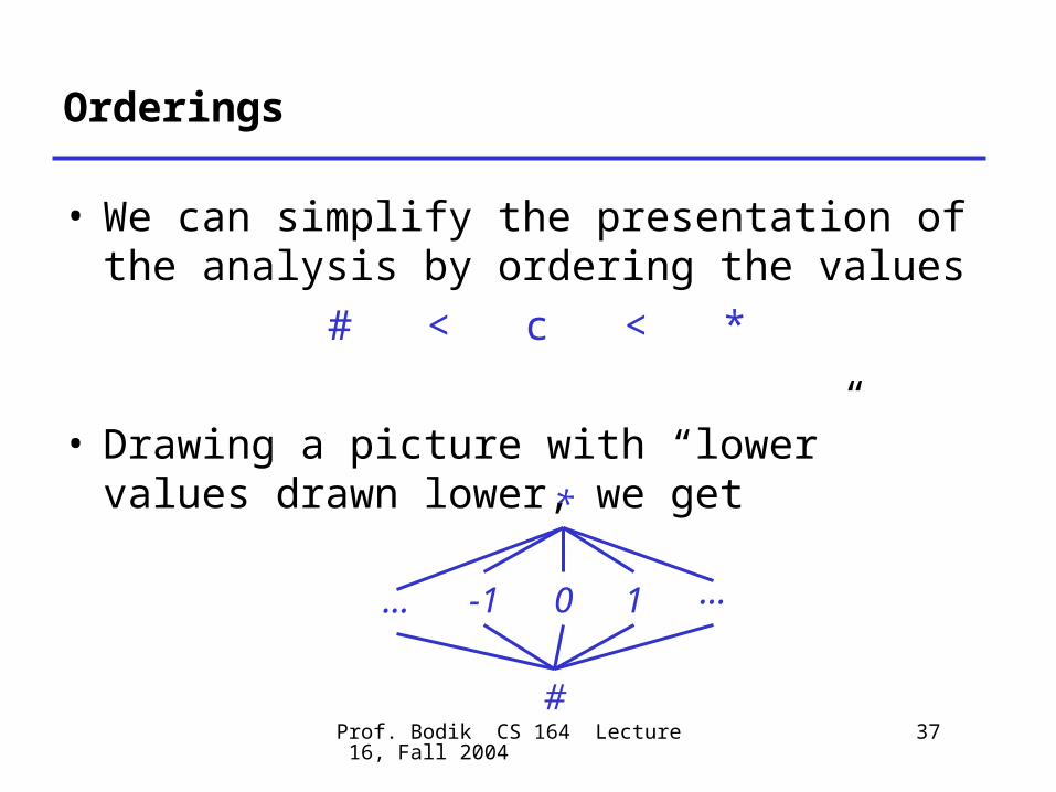
37

Orderings

• We can simplify the presentation of the analysis by ordering the values

# < c < *

• Drawing a picture with “lower” values drawn lower, we get

#

*

-1 0 1… …


38

Orderings (Cont.)

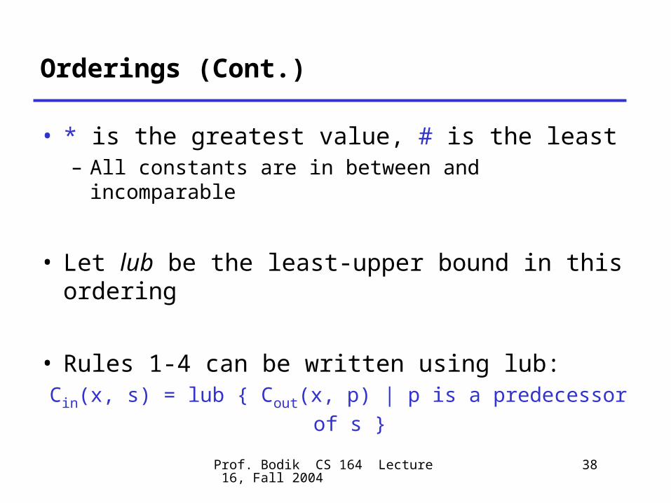
• * is the greatest value, # is the least– All constants are in between and incomparable

• Let lub be the least-upper bound in this ordering

• Rules 1-4 can be written using lub:Cin(x, s) = lub { Cout(x, p) | p is a predecessor of s }


39

Termination

• Simply saying “repeat until nothing changes” doesn’t guarantee that eventually nothing changes

• The use of lub explains why the algorithm terminates– Values start as # and only increase– # can change to a constant, and a constant to *– Thus, C_(x, s) can change at most twice


40

Termination (Cont.)

Thus the algorithm is linear in program size

Number of steps = Number of C_(….) values computed * 2 =Number of program statements * 4


41

Liveness Analysis

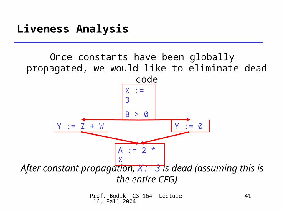
Once constants have been globally propagated, we would like to eliminate dead code

After constant propagation, X := 3 is dead (assuming this is the entire CFG)

X := 3

B > 0

Y := Z + W Y := 0

A := 2 * X


42

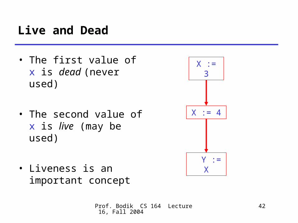
Live and Dead

• The first value of x is dead (never used)

• The second value of x is live (may be used)

• Liveness is an important concept

X := 3

X := 4

Y := X


43

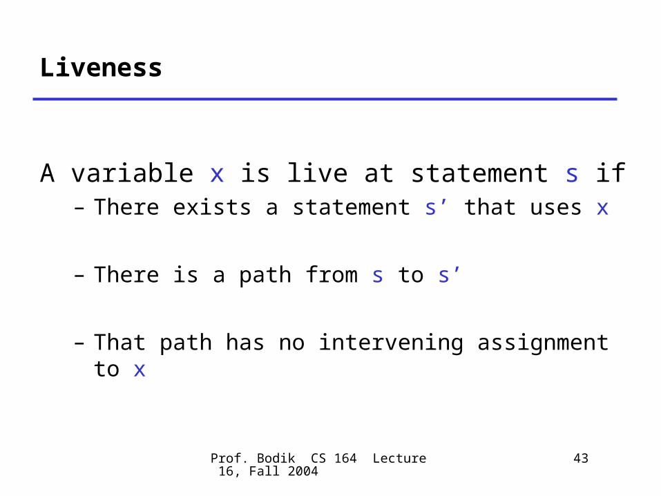
Liveness

A variable x is live at statement s if– There exists a statement s’ that uses x

– There is a path from s to s’

– That path has no intervening assignment to x


44

Global Dead Code Elimination

• A statement x := … is dead code if x is dead after the assignment

• Dead statements can be deleted from the program

• But we need liveness information first . . .


45

Computing Liveness

• We can express liveness in terms of information transferred between adjacent statements, just as in copy propagation

• Liveness is simpler than constant propagation, since it is a boolean property (true or false)


46

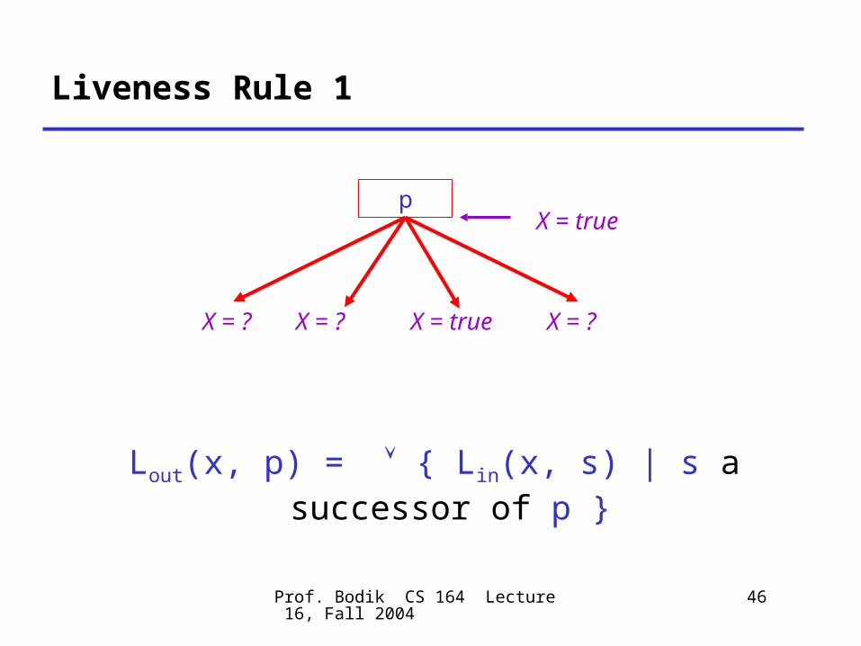
Liveness Rule 1

Lout(x, p) = { Lin(x, s) | s a successor of p }

p

X = true

X = true

X = ?

X = ?

X = ?


47

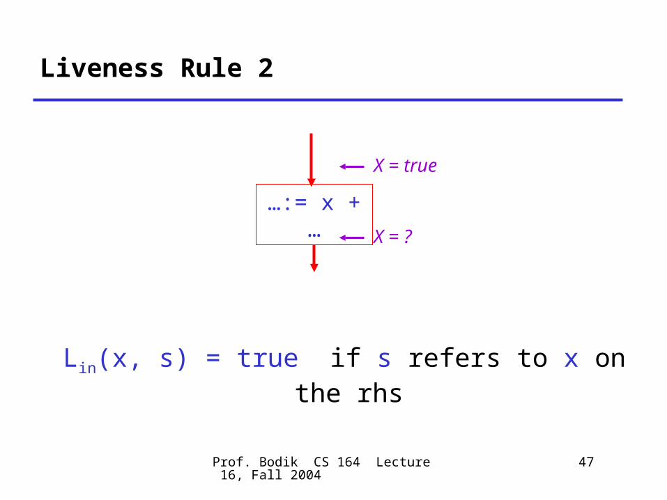
Liveness Rule 2

Lin(x, s) = true if s refers to x on the rhs

…:= x + …

X = true

X = ?


48

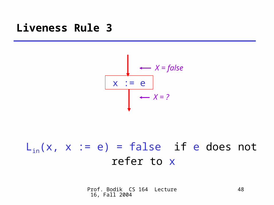
Liveness Rule 3

Lin(x, x := e) = false if e does not refer to x

x := e

X = false

X = ?


49

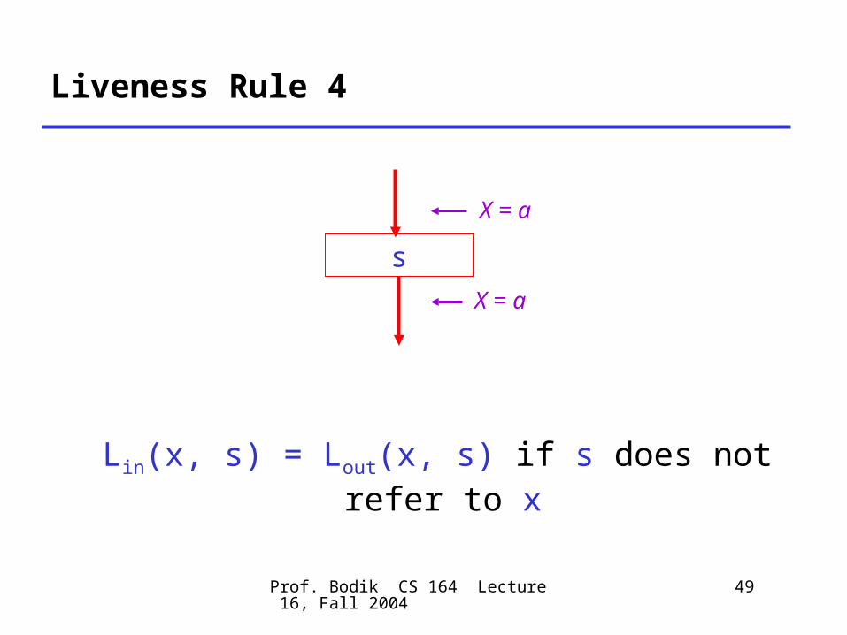
Liveness Rule 4

Lin(x, s) = Lout(x, s) if s does not refer to x

s

X = a

X = a


50

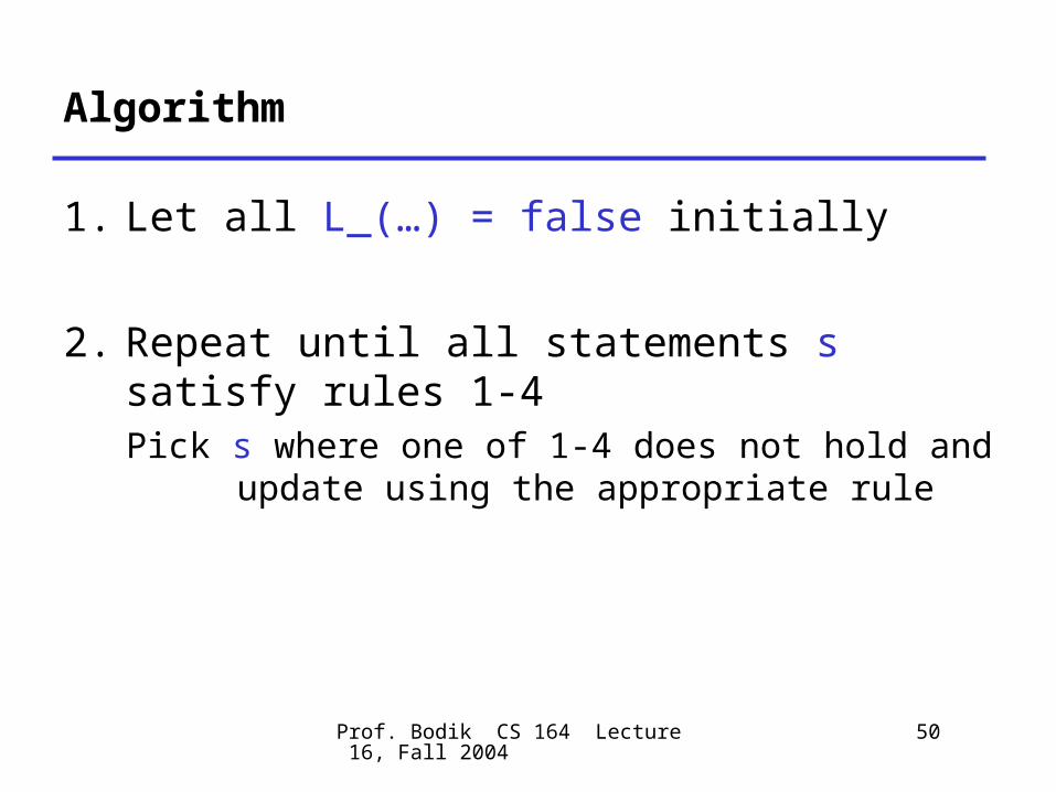
Algorithm

1. Let all L_(…) = false initially

2. Repeat until all statements s satisfy rules 1-4Pick s where one of 1-4 does not hold and update

using the appropriate rule


51

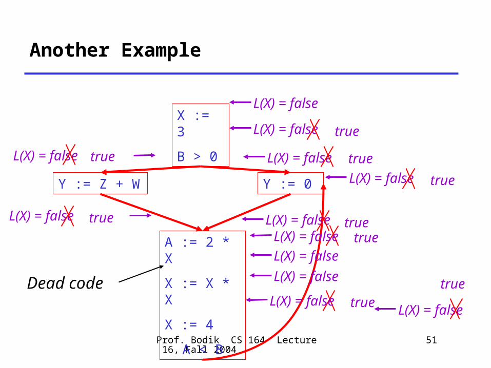
Another Example

X := 3

B > 0

Y := Z + W Y := 0

A := 2 * X

X := X * X

X := 4

A < B

L(X) = false

true

L(X) = false

L(X) = false L(X) =

false

L(X) = false L(X) = false L(X) = false L(X) = false

L(X) = false

L(X) = false

L(X) = false

true true

true

true

true

truetrueL(X) =

false

true

Dead code


52

Termination

• A value can change from false to true, but not the other way around

• Each value can change only once, so termination is guaranteed

• Once the analysis is computed, it is simple to eliminate dead code


53

Forward vs. Backward Analysis

We’ve seen two kinds of analysis:

Constant propagation is a forwards analysis: information is pushed from inputs to outputs

Liveness is a backwards analysis: information is pushed from outputs back towards inputs


54

Analysis

• There are many other global flow analyses

• Most can be classified as either forward or backward

• Most also follow the methodology of local rules relating information between adjacent program points

Documents

Prof. Bodik CS 164 Lecture 16, Fall 20041 Global Optimization Lecture 16