1

Profitability of Momentum and Overreaction Trading Strategies in Switzerland Stock Market

By

Mani Naghavi

Dissertation submitted in partial fulfillment of

MSc in Finance and Banking

Dissertation Supervisor

Professor Elango Rengasamy

June 12, 2012

2

Abstract

Following available literatures on overreaction hypothesis and momentum effect, this research examines the profitability of contrarian and momentum strategies within large cap/blue-chip stocks of Switzerland financial market. Using a high frequency tactical asset allocation, the winner stocks continued to yield a significant large return in one day after portfolio formation and the losers reported insignificant return, hence, momentum is found to be profitable strategy in one-day holding period with an average return of above 14% per annum. A significant contrarian profitability of over 5% is also observed in 3 and 10 days holding period. Furthermore, the result shows Friday and January effect within momentum return in one day holding period.

3

Acknowledgements

I would like to express my gratitude to all those who gave me the possibility to complete this thesis.

I want to begin by acknowledging my supervisor, Dr. Elango Rangasamy, for his great help and support during my study. It would not be an overstatement to say that my experience would have been very different indeed had I not had the fortune of having him as my guide.

I owe a debt of gratitude to my wonderful wife, Shirin, for her vital role, immense support, patience and unwavering love that have been the bedrock upon which our life is built. I can state with some certainty that I would not have been in a position to present this work had it not been for her enabling encouragements and support.

I would like to acknowledge my colleague, Lynnette Gison, who shouldered some of my responsibilities at work helping me to focus on my studies especially during the last weeks before my submission. Special thanks goes to my cousin, Ronak Ahmadlou, for her benevolent support providing data and technical advice. I wish also like to thank my friends, Kamran Solaimanzdeh and Maryam Moghaddam, whom I am greatly indebted to for their valuable tips and companionship during my studies.

Another special thanks goes to my best friend, Ehsan Mostashari, for his unconditional and end-less support and understanding at times when I really needed

Through every stage I had my full stream support from my parents and of course my sister, Nika, whose positive attitude has been a source of inspiration to me. There are no words that adequately express my appreciation and gratitude to them.

4

Table of contents

1. Introduction ...................................................................................................................................... 6  

1.1. Statement of Research Problem ............................................................................................... 8  

1.2. Rational of Study ....................................................................................................................... 9  

1.3. Objective and Research Question ........................................................................................... 9  

1.4. Statement of hypothesis ........................................................................................................... 9  

1.5. Limitation ................................................................................................................................. 10  

2. Literature Review ........................................................................................................................... 10  

2.1. Overreaction Hypothesis and Long Term Contrarian Strategies .................................... 10  

2.2. Non-US Evidence of Long Term Contrarian Strategies .................................................... 18  

2.3. Short-term Momentum Strategies ........................................................................................ 20  

2.4. Contrarian / Momentum in connection with other factors and different markets ....... 22  

3. Sample and Methodology ............................................................................................................. 25  

3.1. About Switzerland’s financial exchange .............................................................................. 25  

3.2. Sample/ Data selection .......................................................................................................... 26  

3.3. Test Procedure (details) .......................................................................................................... 28  

3.4. Descriptive statistics and test of significance ...................................................................... 30  

3.5. Loser, Winner, Contrarian (Momentum) Statistical Significance .................................... 30  

3.6. Seasonality in returns of momentum and contrarian effect ............................................. 30  

4. Result and Analysis ....................................................................................................................... 31  

4.1 Different HPR returns, strategies profitability and significance ....................................... 31  

4.2 Seasonality in profitability of momentum a K=1 ................................................................ 32  

4.3 Regression Analysis ................................................................................................................. 34  

5. Conclusion ....................................................................................................................................... 35  

6. References (bibliography) ............................................................................................................ 36  

7. List of tables .................................................................................................................................... 39  

Table 1- Sampling of Observed Pricing Anomalies .................................................................. 39  

5

Table 2- SMI Members Companies .............................................................................................. 39  

8. Appendices ...................................................................................................................................... 40  

Appendix 1. Swiss market graphic representation of different indices ..................................... 40  

Appendix 2- Average Arithmetic and Geometric Mean returns to trading strategies ............ 41  

Appendix 3- Descriptive statistics for portfolio of winners, losers and zero cost strategy ..... 42  

Appendix 5 –Test of significance for mean returns of losers and winners in difference holding periods (t-test for hypothesized mean of zero) ............................................................... 46  

Appendix 6- Paired Sample t-test for Momentum and Contrarian strategies .......................... 50  

Appendix 7- Yearly and Monthly Decomposition of Momentum return (k=1) ....................... 53  

Appendix 8- Daily Decomposition of Momentum Strategy Average returns (k=1) ................ 54  

6

1. Introduction

Market efficiency has been a very attractive area in finance and it can be traced back to Bachelier (1900) and the empirical research done by Cowles (1933). However, the terminology of efficient market hypothesis (EMH) is associated with the work of Eugene Fama in his PhD thesis in 1960’s. Fama (1970) summarizes his idea of market efficiency as follows: “a market in which prices always ‘fully reflect’ available information is called ‘efficient’”. EMH at its core states that “in an informationally efficient market, price changes must be unforecastable if they are properly anticipated, i.e. if they are fully incorporate the expectations and information of all market participants” Campbel, Lo and MacKinlay (1997). Also, a market is said to be efficient with respect to an information-set, when releasing that information would cause no movement in price of that asset. In such a market it is implied that it would be impossible to make economic significant profit by trading on the basis of the information set available to all market participants. This is mainly due to the fact that in an efficient market, at any point in time the prices would already incorporate the effect of that information set or will adjust very quickly to reflect the value of information set.

There are usually two approaches to assess the market efficiency as outlined by McMillan et al. (2011). One would either measure risk-adjusted profit earned by “market professionals” such as profit earned by mutual funds or hypothetically tests if trading on the basis of a set of known information would result in a significant profit (abnormal profit) over the market return. The market efficiency has been introduced in three forms: weak form, semistrong-form and strong form in which information reach is narrowed down from weak to strong form. In weak-form market efficiency, the information set includes only the historical prices and volume whereas the semistrong-form efficiency includes all public available information to all market participants (i.e. news, accounting data and etc.). The information set in strong form includes all information known to any market participant (public and private information). This means that by accessing the historical prices, public and private information one cannot consistently and significantly achieve superior returns over the market. It is important to note that the concept of market efficiency is a relative subject and financial markets are not entirely efficient or inefficient but rather falling within a range between the two extremes.

Considerable evidence shows, contrary to market efficiency theory, there are a number of well-researched inefficiencies, anomalies, which would cause the mispricing of the securities. Market anomalies are challenging the notion of efficiency in a financial market. The anomalies are ranging from January effect, size effect to cross-sectional and other mispricing effects. McMillan et al. (2011) have provided a non-exhaustive list of well-known market anomalies and have categorized them into three different categories: time series

7

anomalies, cross- sectional anomalies and others. Table 1 provides a more elaborate classification within each category. This research in particular looks into time series anomaly of momentum and overreaction.

The most important and well-documented anomalies within the time series group are the overreaction and momentum anomalies. DeBondt and Thaler (1985) have published one of the earliest studies of overreaction where they based their study on the hypothesis that the investor would overreact to release of public information, i.e. overreaction hypothesis. Therefore stock prices would become overpriced (underpriced) as a result of good (bad) information. They have coined the term “overreaction” for this anomaly. Following the individual’s overreaction, they have proposed a strategy, which is contrary to other investor’s naïve strategy of investment in stocks. This means that while one can assume (naïve strategy) continuation in stock prices, contrarian strategy assumes a reversal in prices. These naïve strategies might range from extrapolating past earning growth far into the future, to assuming a trend in stock prices, to overreacting towards good or bad news, or to simply equating a good investment with a well-run company irrespective of price” (Lakonishok et. al. 1994). Predictability of asset returns has been of a great interest to researchers and professional traders dating back to pre-1960 as described by Conrad and Kaul (1998) and number of researchers argued that time series patterns of prices are due to market inefficiency and can be exploited and used to beat the market, hence, creating an abnormal profit.

Contrarian strategy would identify the winner and loser stocks based on their past 3 years returns. They sold the winners short and went long on the losers in anticipation that the winner (loser) stocks were overpriced (underpriced) and will revert to their intrinsic mean value eventually. The contrarian (overreaction) strategy proved to be profitable in long horizon in US equity market, some other international financial markets as well as bond markets; DeBondt and Thaler (1985, 1987), Lakonishok(1996) and others. However, Jagadeesh (1990), Chopra, Lakonishok and Ritter (1992) demonstrated that the contrarian strategy yields significant and positive return in both very short period i.e. weekly and long horizon i.e. three to five years.

On the other hand and intuitively contrasting to contrarian logic, momentum strategy in stock market follows continuation in asset prices return rather than reversal. Momentum refers to short-term price patterns where a continuation in stock prices is observed in a market. Similar to contrarian strategy, momentum pattern in price of an asset is also challenging the market efficiency idea and is considered as an anomaly to EMH. Jagadeesh and Titman (1993, 2001), Chan, Jagadeesh and Lakonishok (1996) and others investigated the momentum effect in US stocks and found that investors on may underact to good (bad)

8

news and therefore, prices would follow a continuation pattern which can be exploited within a medium term (three to six month) in order to create abnormal profit. This strategy involves buying winners and selling losers to make an arbitrage profit.

Notably, many researchers tried to explain the source of momentum profitability and decomposition of profit created based on this notion of short selling the losers and taking long positions on the winners. Fama French (1996) demonstrated that even their famous three-factor model is also unable to explain the short-term return continuation. Maskowitz and Grinblatt (1999) found that industry effect might be the source of momentum profitability, i.e. selling stocks from losing industry and buying from the winning industry seemed to be highly profitable, and hence, the industry effect was a part of profitability created by momentum investing. Other studies found the effect of size and seasonality to contribute to the profitability of momentum or contrarian strategies; Zarwin (1989), Jagadeesh and Titman (1993) DeBondt and Thaler (1987) and others.

While many studies of overreaction and contrarian trading strategies have been done in United States market, to my best knowledge, the momentum and overreaction in Switzerland financial market is not tested independently within the last couple of years. Therefore, this research tries to identify if there is profitability in momentum/ overreaction within Switzerland financial market. The stocks chosen for this study are the 20 blue chip stocks of Switzerland. By such selection, the thin trading bias could be avoided due to the fact that the stocks are the highly liquid and large cap stocks of the market. In addition, the size effect does not seem to undermine the profitability of the strategy since all of the participants are chosen from the large cap stocks.

The trading strategy chosen for this research is a high frequency trading which ranks stocks on daily basis and form portfolio of losers and winners accordingly. The stock returns are monitored in period of 1, 3, 10, 30, 90, 120, and 250 day after each day of formation. The trading strategy would find a profitable momentum effect in 1 day after formation and contrarian effect in 3 days and 10 days after formation period. This study also present a weekday, year and month breakdown for raw return in 1 day momentum return.

1.1. Statement of Research Problem

This research will look into the momentum or contrarian strategy profitability within the blue chip stocks of Switzerland’s financial market from 1992 to 2011.

9

1.2. Rational of Study

Since both momentum and contrarian investment styles are proven to coexist in financial markets throughout different time horizons, this study will explore to find economic and statistical significant profit by using applying these strategies within blue chip stock members in Switzerland financial markets. On the one hand, the study will contribute to the well-researched area of contrarian and momentum time series anomalies but within new financial markets. On the other hand, the methodology (event study) will trade stock on everyday basis, which is a high frequency tactical asset allocation that may be of an interest to high frequency traders and fund managers in European financial markets.

1.3. Objective and Research Question

The aim of the research is to test high frequency tactical asset allocation, which invests in top/ bottom blue chip stocks in Switzerland’s financial market in order to make a profit higher than the market. The objectives of the research could be narrowed down into following steps:

• To monitor the winners and losers portfolio on daily basis

• To determine the profitability of winners, losers portfolio throughout the study period

• To test the statistical significance of each portfolio

• To explore the evidence of momentum/ contrarian profitability within SMI member stocks

• To decompose and demonstrate the source of profitability in such strategies in this market

1.4. Statement of hypothesis

The research hypothesis can be formulated as a general hypothesis while other sub- hypothesis are also defined and tested within the methodology and results part of this research. The general hypothesis of this research can be summed into the following hypothesis:

!!=There is no significant profit to trading strategy of momentum and contrarian using past returns within blue chip stocks of Switzerland market

!!= There is a significant profit to trading strategy of momentum and contrarian using past returns within blue chip stocks of Switzerland market.

10

The sub hypotheses that are further tested are the profitability to winners and losers portfolio within each trading intervals, which are provided in data and methodology chapter.

1.5. Limitation

First limitation to this study has been the limited access to historical market data through third party. Secondly, access to information on market microstructure (i.e. bid-ask spread, trading cost, brokerage fees and etc.) Therefore, the returns to these strategies are reported without consideration of transaction costs. Third and most importantly, the problem of non-normality in daily returns, which restricted the use of single market, model (i.e. CAPM) due to underlying normality assumption in such models.

The remainder of this research is structured as follows: Chapter 2, provides a detailed account of overreaction hypothesis and momentum literatures in USA financial market and a few other studies of overseas markets including the source of profitability in such strategies as well as criticism and methodological issues. Chapter 3, describe a brief description of the Switzerland financial market as well as sample selection and methodology. Chapter4, summarize the findings and provide explanations for such findings followed by Chapter 5, conclusion of the research findings.

2. Literature Review

2.1. Overreaction Hypothesis and Long Term Contrarian Strategies

One of the first studies of overreaction hypothesis is done by De Bondt and Thaler (1985) 1 and due to the fact that any further studies of overreaction hypothesis is an attempt to explain, test, refute, expand or challenge their idea, it is important to provide a detailed account of their research idea and methodology. Their research is based upon the simple fact that people overreact to unexpected and dramatic news events and as a result the asset prices will become overvalued (undervalued). Although not a direct study to gauge market efficiency, their research investigated whether this behavioral pattern could be expanded at the market level and can be predicted and exploited to make abnormal profit. According to authors, such overreaction is driven by individual’s tendency “to overweight the recent information and underweight prior (or base rate) data” which is in contrast with Bayes’ rule. Bayesian model of investment management suggests that all information should be weighted and factored in the decision making process according to their importance.

1 As described by Merton (1985), this study has been “particularly noteworthy because it represents a first attempt to a formal test of cognitive misperceptions theories as applied to general stock market”.

11

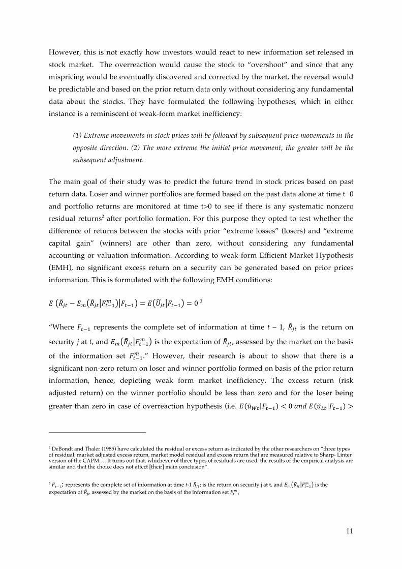
However, this is not exactly how investors would react to new information set released in stock market. The overreaction would cause the stock to “overshoot” and since that any mispricing would be eventually discovered and corrected by the market, the reversal would be predictable and based on the prior return data only without considering any fundamental data about the stocks. They have formulated the following hypotheses, which in either instance is a reminiscent of weak-form market inefficiency:

(1) Extreme movements in stock prices will be followed by subsequent price movements in the opposite direction. (2) The more extreme the initial price movement, the greater will be the subsequent adjustment.

The main goal of their study was to predict the future trend in stock prices based on past return data. Loser and winner portfolios are formed based on the past data alone at time t=0 and portfolio returns are monitored at time t>0 to see if there is any systematic nonzero residual returns2 after portfolio formation. For this purpose they opted to test whether the difference of returns between the stocks with prior “extreme losses” (losers) and “extreme capital gain” (winners) are other than zero, without considering any fundamental accounting or valuation information. According to weak form Efficient Market Hypothesis (EMH), no significant excess return on a security can be generated based on prior prices information. This is formulated with the following EMH conditions:

!   !!" − !! !!" !!!!! !!!! = ! !!" !!!! = 0 3

“Where !!!! represents the complete set of information at time t – 1, !!" is the return on

security j at t, and !! !!" !!!!! is the expectation of !!", assessed by the market on the basis

of the information set !!!!! .” However, their research is about to show that there is a significant non-zero return on loser and winner portfolio formed on basis of the prior return information, hence, depicting weak form market inefficiency. The excess return (risk adjusted return) on the winner portfolio should be less than zero and for the loser being

greater than zero in case of overreaction hypothesis (i.e. ! !!" !!!! < 0  !"#  ! !!" !!!! >

2 DeBondt and Thaler (1985) have calculated the residual or excess return as indicated by the other researchers on “three types of residual; market adjusted excess return, market model residual and excess return that are measured relative to Sharp- Linter version of the CAPM…. It turns out that, whichever of three types of residuals are used, the results of the empirical analysis are similar and that the choice does not affect [their] main conclusion”.

3 !!−1; represents the complete set of information at time t-1 !!"; is the return on security j at t, and !! !!" !!!!! is the expectation of !!" assessed by the market on the basis of the information set !!!!!

12

0) while EMH would suggest that there loser/ winner would not produce any non-zero risk

adjusted return ! !!" !!!! = ! !!" !!!! = 0.

In their test procedure, they have opted stocks on New York Stock Exchange (NYSE) from January 1926- December 1982 (56 years) and they have considered an equally weighted arithmetic average of all stock return as the market index. They have used 16 non-over lapping portfolio formation periods of 3 years, starting from Dec 1932, 1935, … up to January 1975. For each stock to be qualified for consideration in such portfolios there should be at least 85 months of monthly data available. That explains why 1926 is not considered as the starting point of the study. First, stocks residual monthly returns (return in excess of market index is reported) are calculated for 72 months starting in 1930 and ending in 1975 (i.e. 16 non-over-lapping periods). Stock residual returns are categorized in portfolio of losers and winners (top and bottom 35 best/ worst performing stocks are considered in each portfolio). For the next 36 months (three years), the cumulative average return of each portfolio is calculated and reported in their test period. A detailed account of such process is summarized here in order to portrait a better understanding of such event study.

1. Residual returns are calculated in a process, which determines that which stock qualifies to be in the study. The process starts with stocks that at least have a monthly return for 85 months without any missing value. Then starting from January 1930, stocks that appear to have the next 72 months recorded return will be considered to be included in the study. This process will be repeated 16 times (i.e. Jan 1930, 1933, …, 1975) in order to determine which stocks are to be included in the study. Any stocks missing value after 85 months should be eliminated from the study.

2. From December 1932 past residual returns of the last 36 months (t=-35 to t= 0) are calculated and portfolio of winner and losers are ranked based on cumulative

residual returns (!!!). Based on the !!!, the top/ bottom 35 stocks are forming the

winner/ loser for the 16 non-overlapping “portfolio formation periods” from December 1932, December1935… December1977.

3. Test period starts in January 1933 by calculating the next 36 months (t=1 to t= 36). The cumulative average residual returns for all stocks in the portfolio are calculated

(denoted !"#!,!,!    !"#  !"#!,!,!) in each study periods (i.e. 16 study periods; January 1933, January 1935 …January 1978).

4. Using CARs, the average CARs are calculated for all 16 test periods for the winner

and the loser’s portfolio separately and denoted !"!#  !,! and !"!#!,!. For

overreaction to be present the following condition i.e. !"!#!,!   − !"!#  !,! > 0 needs to be met. In order to see if there is a statistically significant different between loser

13

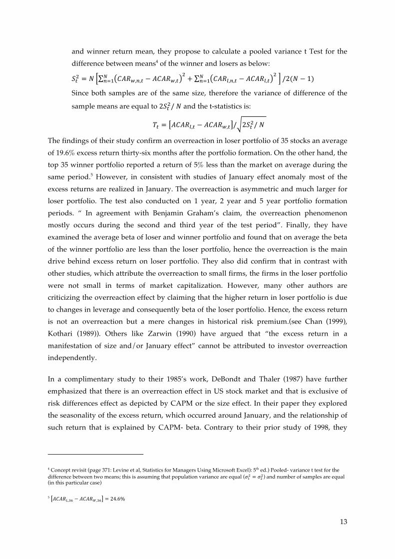
and winner return mean, they propose to calculate a pooled variance t Test for the difference between means4 of the winner and losers as below:

!!! = ! !"#!,!,! − !"!#!,!!!

!!! + !"#!,!,! − !"!#!,!!!

!!!   /2(! − 1)

Since both samples are of the same size, therefore the variance of difference of the

sample means are equal to 2!!!/  ! and the t-statistics is:

!! = !"!#!,! − !"!#!,! / 2!!!/  !  

The findings of their study confirm an overreaction in loser portfolio of 35 stocks an average of 19.6% excess return thirty-six months after the portfolio formation. On the other hand, the top 35 winner portfolio reported a return of 5% less than the market on average during the same period.5 However, in consistent with studies of January effect anomaly most of the excess returns are realized in January. The overreaction is asymmetric and much larger for loser portfolio. The test also conducted on 1 year, 2 year and 5 year portfolio formation periods. “ In agreement with Benjamin Graham’s claim, the overreaction phenomenon mostly occurs during the second and third year of the test period”. Finally, they have examined the average beta of loser and winner portfolio and found that on average the beta of the winner portfolio are less than the loser portfolio, hence the overreaction is the main drive behind excess return on loser portfolio. They also did confirm that in contrast with other studies, which attribute the overreaction to small firms, the firms in the loser portfolio were not small in terms of market capitalization. However, many other authors are criticizing the overreaction effect by claiming that the higher return in loser portfolio is due to changes in leverage and consequently beta of the loser portfolio. Hence, the excess return is not an overreaction but a mere changes in historical risk premium.(see Chan (1999), Kothari (1989)). Others like Zarwin (1990) have argued that “the excess return in a manifestation of size and/or January effect” cannot be attributed to investor overreaction independently.

In a complimentary study to their 1985’s work, DeBondt and Thaler (1987) have further emphasized that there is an overreaction effect in US stock market and that is exclusive of risk differences effect as depicted by CAPM or the size effect. In their paper they explored the seasonality of the excess return, which occurred around January, and the relationship of such return that is explained by CAPM- beta. Contrary to their prior study of 1998, they

4 Concept revisit (page 371: Levine et al, Statistics for Managers Using Microsoft Excel): 5th ed.) Pooled- variance t test for the difference between two means; this is assuming that population variance are equal (!!! = !!!) and number of samples are equal (in this particular case)

5 !"!#!,!" − !"!#! ,!" = 24.6%

14

opted for overlapping “formation period” and “test period“ over 120 months6 from 1926 up to January 1973, hence resulting in 48 over lapping test periods. Another distinction in methodology seems to be the choice of the winner and the loser portfolio which is arbitrarily chosen top 50-best/ worst performing stocks whereas the previous study considered top/ bottom deciles for selection of winner and losers in each portfolio.

They have also calculated the beta for both up and down market7, i.e. when market risk premium was positive and negative, and they found that the arbitrage portfolio8 (zero investment portfolio without considering transaction cost) has a positive beta in up market and a negative beta in down market, which in their view reduced the risk of the strategy. Notably, they found that the beta of the arbitrage portfolio reported as 0.220 which is insufficient to explain the average annual return of 9.2% and a positive and significant

!  !"  5.9% was also suggestive of an abnormal performance. Hence, they concluded that the risk difference is not the primary cause of such overreaction. They further demonstrated that small firms is found to be generating excess returns even if the losing firm is removed form the small firm group.

Ball and Kothari (1989) found a negative serial correlation in “relative (market-adjusted)” stocks returns. The classical explanation of such serial correlation could be summed into two competing determinants: (1) market mispricing and (2) changing expected return in an efficient market. For this reason, they have reexamined the data of DeBondt and Thaler (1985,1987), a contrarian strategy of investing in losers and short selling of the winners, and found that if adjustment for risk were considered (time varying beta vs. constant Beta) there would not be any substantial abnormal profit. The serial correlation is “due largely to changing relative risks and thus changing expected returns. In addition, they demonstrated that the evidence of negative serial correlation is not consistent with stock market mispricing.

Ball et al. (1995) revisited the methodology and data set of DeBondt and Thaler (1985 and 1987) and raised some serious criticism about their findings. They debated that the event study used by Debondt and Theler (1985,1987); Chan (1988); Ball and Kothari (1989); Chopra lakonishok and Ritter (1992) suffered from severe performance measurement problems. Notably, the profit of the contrarian investment strategy would come from investment in

6 a 60 months formation followed by a 60 months of test

7 !!" =  !! + !!"(!!" − !!")!   + !!"(!!" − !!")(1 − !), Where D is the dummy variable which equals one when !!" > 0 and zero when !!" < 0, !!" is the arbitrage portfolio and !!"and !!"   are up and down market betas

8!!" =  !!" − !!" , Where !!"  !"#  !!" is the average return of losers and winner portfolios in each period

15

low-priced, right-skewed return portfolios, which are highly sensitive to market microstructure effect (spread, liquidity and brokerage costs). The return to loser portfolio was mostly from lowest-price quartile of loser with average price of $1.04 and hence it would be sensitive to market microstructure. Furthermore, the choice of end-period shift from year-end to June-end portfolio formation showed that not only contrarian effect is not independent but also the loser portfolio lost 31% of its value. The change in arbitrary calendar starting point was, according to the authors, suggestive of a performance measurement problem. In addition, the stocks were shown a negative 2.5% Jensen’s alpha (See Chan 1988; Ball and Kothari 1989) when measuring the abnormal performance on June-end portfolio whereas the December-end portfolio yield an alpha of positive 4.5%, hence, one can argue that the arbitrarily chosen intervals were the source of abnormal profit and cast doubt on the robustness of the results obtained by DeBondt and Thaler (1985, 87).

Chopra, Lakonishok & Ritter (1992) CLR (1992) also looked into the evidence of overreaction effect in the US stock market. Their approach is a comprehensive and complimentary to prior works done by DeBondt and Thaler (1985), Chan (1988), Ball and Khothari (1989) and Zarowin (1990). In this study they examined overreaction evidence based on prior portfolio performance as well as the effect of the beta, size, seasonality and multiple regression factor to explain and present an independent and economically significant overreaction effect. For data set, they used the NYSE all stocks from 1926 to 1986 (40 years). They have ranked the stocks based on a 5-year buy and hold return into twenty portfolios. Contrary to the study of Debondt and Thaler (1985), the ranking periods and post ranking periods are chosen to be over-lapping periods of five years, which resulted in 52 periods of observation.9 This would seem to introduce a problem of independence in the time series data, hence, causing a serial correlation and adjustment of the fourth degree autocorrelation in time series analysis as suggested in their footnotes. Perhaps extent of such impact and the way the adjustment for the serial dependence is done are not reported in this study and would be outside the scope of this paper.

In order to estimate the market model coefficient, they used Ibbotson’s (1975) returns across times and security using (RATS)10 procedure. Each portfolio is assigned to event year -4 to +5 (i.e. the first year of ranking period being year number -4, the first year of post-ranking

9 (Overlapping) ranking period: 1926-1930, 1927-1931, … , 1977,1981

(Overlapping) post ranking period: 1931-1935, 1932,1936, … , 1982-1986

10 Regression Analysis of Time Series (RATS) is a statistical and time series analysis software package

16

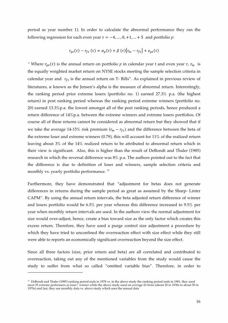
period as year number 1). In order to calculate the abnormal performance they ran the

following regression for each even year ! = −4,… , 0,+1,…+ 5 and portfolio p:

!!" ! − !!"   ! = !! ! + !   ! !! − !!" + !!" !

“ Where !!" ! is the annual return on portfolio p in calendar year t and even year !, !! is

the equally weighted market return on NYSE stocks meeting the sample selection criteria in

calendar year and !!" is the annual return on T- Bills”. As explained in previous review of

literatures, ! known as the Jensen’s alpha is the measure of abnormal return. Interestingly, the ranking period prior extreme losers (portfolio no. 1) earned 27.3% p.a. (the highest return) in post ranking period whereas the ranking period extreme winners (portfolio no. 20) earned 13.3%p.a. the lowest amongst all of the post ranking periods, hence produced a return difference of 14%p.a. between the extreme winners and extreme losers portfolios. Of course all of these returns cannot be considered as abnormal return but they showed that if

we take the average 14-15% risk premium (!! − !!") and the difference between the beta of

the extreme loser and extreme winners (0.79), this will account for 11% of the realized return leaving about 3% of the 14% realized return to be attributed to abnormal return which in their view is significant. Also, this is higher than the result of DeBondt and Thaler (1985) research in which the reversal difference was 8% p.a. The authors pointed out to the fact that the difference is due to definition of loser and winners, sample selection criteria and monthly vs. yearly portfolio performance. 11

Furthermore, they have demonstrated that “adjustment for betas does not generate differences in returns during the sample period as great as assumed by the Sharp- Linter CAPM”. By using the annual return intervals, the beta adjusted return difference of winner and losers portfolio would be 6.5% per year whereas this difference increased to 9.5% per year when monthly return intervals are used. In the authors view the normal adjustment for size would over-adjust, hence, create a bias toward size as the only factor which creates this excess return. Therefore, they have used a purge control size adjustment a procedure by which they have tried to unconfined the overreaction effect with size effect while they still were able to reports an economically significant overreaction beyond the size effect.

Since all three factors (size, prior return and beta) are all correlated and contributed to overreaction, taking out any of the mentioned variables from the study would cause the study to suffer from what so called “omitted variable bias”. Therefore, in order to

11 DeBondt and Thaler (1985) ranking period ends in 1978 vs. in the above study the ranking period ends in 1981, they used most 35 extreme performers as loser/ winner while the above study used on average 43 firms (about 20 in 1930s to about 50 in 1970s) and last, they use monthly data vs. above study which uses the annual data

17

incorporate the 3 factors at once they have incorporated a multiple regression whereby all three variables are considered. The independent overreaction effect was reported as 5%, which showed a prolonged January seasonal effect as seen in findings of the other authors. The overreaction is also not “homogenous” across the size groups and the smaller firms winner and losers tend to overreaction in larger magnitude than the larger cap portfolios.

This study had several implications in understanding the market behavior. First, authors had mad an inference that the individuals, which mostly hold the small cap stock, tend to overreact more than the institutions that hold large-cap stocks. Second, if the mispricing is due to overreaction and the pattern seems to be repeated why it is not exploited and removed by the arbitrageurs? The answer to this would be the fact that according to Shleifer and Vishny (1991 quoted in CLR 1991), “smart money investors are exposed to opportunity cost if there is no certainty that mispricing will be corrected in a timely manner” hence, they focus on short term arbitrage opportunities rather than long term ones.

While Debondt and Thaler (1985 and 1987) made a very good first attempt to portrait overreaction hypothesis, there have been so many skeptics to their interpretation of the result. Particularly, Chan (1988) has re-investigated a different sample12 within the same sample space using the same event study and found that the contrarian strategy would yield an insignificant return over the market, which may not be interpreted as evidence for market overreaction. The risk for winner and loser stocks will not remain constant over time. ”The risk of this strategy appears to be correlated with the level of expected market-risk premium”. Hence, the abnormal returns compensate with the additional implied risk. They have shown that the loser beta will go up after experiencing a dip in return and the winner beta will go down after a rise in their return. In their view, it would be also wrong to consider the average beta for risk measurement of the portfolio as both the average betas and market risk premium “might respond to some common state variables and are thus correlated”. They further emphasize that this strategy may pick the riskier stocks when the expected market risk premium is high, “probably because losers suffer larger losses at economic downturns than upturns, hence the strategy may result an “above –market” returns in compensation for taking higher risk.

While the small firms, risk differences and January or other calendar effects may bias long-run overreaction/ contrarian effect, Zarwin (1989) argued that there is an efficient market anomaly for short-run contrarian effect. He arranged the portfolios by observing top10% /worst 10%performer over one-month return in formation period followed by one month of

12 they have ranked portfolios of winners and loser based on both top/ bottom decile as well as 35 top/bottom best performing

18

a test period. He found out that during the extreme performance month winners would over outperform the losers by 33.5% but in the following month losers would outperform the winners by statistically significant 2.8% per year. Of course, the raw returns were only indicative of possibility of a contrarian effect but cannot be inferred upon as overreaction without further test. Consequently, he had controlled the risk differences of winner and losers portfolio using a regression model as used by De Bondt and Thaler (1987) and found appositive alpha of 2.5%, suggestive that the losers outperformed the winners. Obviously, like many other studies of the overreaction/ contrarian effect, the January effect was also dominant by abnormal return in excess of 5.5% for January only.

In any study of momentum and contrarian effect, the general assumption is that people would overreact or underreact to favorable and unfavorable information. This would result in over valuation/ under valuation of assets return and consequently provide an arbitrage opportunity. Study of market overreaction is an attempt to generalize this behavioral theory and expand it to a market behavior..

2.2. Non-US Evidence of Long Term Contrarian Strategies

Following Debodt and Thaler (1985) footsteps, many other authors have tested the evidence of overreaction hypothesis and in particular contrarian strategy in other non- US stock market Clare and Thomas (1995) investigated a property of mean reversion in stocks known as overreaction hypothesis. They examined evidence of the overreaction hypothesis in UK stock market13. As the data sample, they opted for 1000 randomly selected stocks in any one year listed in London Stock Exchange from 1955 to 1990 (i.e. 36 years). They demonstrated that the return of previously poor performing stocks, so called the “losers”, outperforms the return of the stocks that had relatively performed well, so called the “winners”. They followed the same “standard event study” as used by DeBondt and Thaler (1985). The winner and loser portfolio formation followed a relatively similar procedure as the other study of momentum, contrarian/ overreaction strategy: Firstly, they have taken the monthly “dividend adjusted” returns and categorized the stocks as per their excess returns over the

market return (!. !.    !! = !! − !!) into periods of 12, 24, and 36 months14. Secondly, they have calculated the average return of each stock based on each portfolio’s length i.e. n= 12, 24 or 36.15 Thirdly, based on these average returns they defined the top 20% best performing,

13 Overreaction hypothesis refers to a property of mean reversion related to investor’s overreaction to information… [Reference required]

14!!"     = !!" − !!" where: t= 1,…n i=1,…,1000 n=12, 24 or 36

15 !!= !! !!"!

!!!

19

i.e. top “quintile”, as the winners and bottom 20 %, i.e. bottom “quintile” as the losers for each time horizon of study i.e. 12, 24 or 36 month.

The definition of losers and winners appears to be arbitrary (i.e. top/ bottom decile, quartile and etc.) in many of studies for momentum/contrarian strategy. Clare and Thomas’s (1995) study utilizes top/ bottom quintile in their categorization of the winner and loser portfolio in order to incorporate a relatively “well diversified portfolio”. Another important aspect of this study was that, they have chosen “non- overlapping” study periods in formation of their portfolio. Based on 36 years of data, calculating returns on one-year intervals would result in 18 non-overlapping one-year observation periods and then 9 and 6 non-overlapping 2-year and 3-year observation periods when returns are calculated on two-year and three-year basis.

Equally weighted averages of portfolio return were then calculated to report the return on

the winner portfolio (!!!) and the looser portfolio !!! , which resulted in a positive

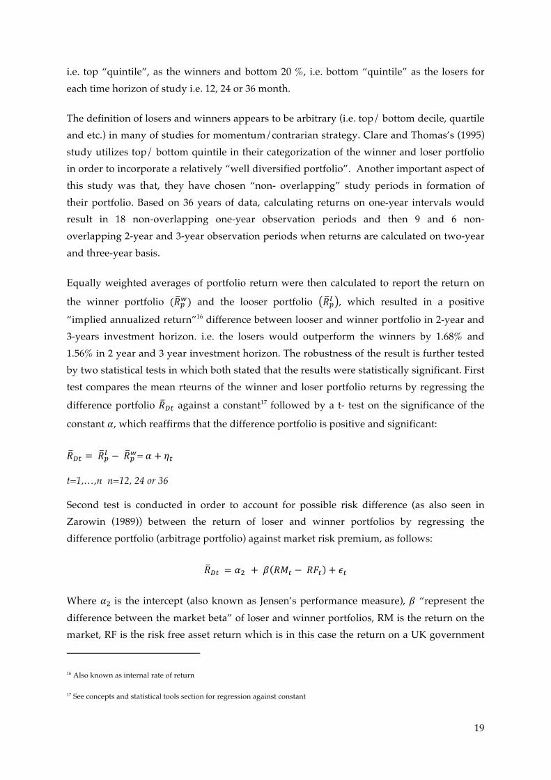
“implied annualized return”16 difference between looser and winner portfolio in 2-year and 3-years investment horizon. i.e. the losers would outperform the winners by 1.68% and 1.56% in 2 year and 3 year investment horizon. The robustness of the result is further tested by two statistical tests in which both stated that the results were statistically significant. First test compares the mean rteurns of the winner and loser portfolio returns by regressing the

difference portfolio !!" against a constant17 followed by a t- test on the significance of the

constant !, which reaffirms that the difference portfolio is positive and significant:

!!" =  !!! −  !!!=  ! + !!

t=1,…,n n=12, 24 or 36

Second test is conducted in order to account for possible risk difference (as also seen in Zarowin (1989)) between the return of loser and winner portfolios by regressing the difference portfolio (arbitrage portfolio) against market risk premium, as follows:

!!"   = !!     +  ! !"! −  !"! + !!

Where !!    is the intercept (also known as Jensen’s performance measure), ! “represent the difference between the market beta” of loser and winner portfolios, RM is the return on the market, RF is the risk free asset return which is in this case the return on a UK government

16 Also known as internal rate of return

17 See concepts and statistical tools section for regression against constant

20

Three month T- Bill) and !! is the white noise error term. A significant high value of !!     confirms that there is a risk adjusted overreaction effect in the market. A significantly different from zero beta means that the difference in systematic risk explains the difference in the returns and a significant positive value means that the losers may entail more systematic risk than the winners.

The results confirm that in the 2-year and 3-years investment horizon there is an overreaction in UK stock market. However, in the 1-year study period their results not only does not demonstrated an overreaction but also showed a continuation in return of losers and winners which further confirmed the findings of Debondt and Thaler (1985) that the losers would remain loser for short horizon. This continuation trend is also called

momentum effect. The coefficient alpha  (!) is positive and significant. Furthermore, the implied annualized return is also positive for 2 year and 3 years horizon with value of 1.68% and 1.56% return. This is confirming an overreaction in UK stock market. However, after adjustment for size effect and January effect, the results confirmed that the overreaction is mostly due to return in January and losers tend to belong to the smaller firm category, hence, the difference in return, although not may be economically significant in their view, could be attributed to small firm effect and not an independent overreaction effect.

2.3. Short-term Momentum Strategies

Another import time series anomaly is the momentum effect; the tendency of the stocks prices/ returns to continue in the same direction in the subsequent period for a short-term period of time after a period of positive and high returns. One of the first researchers to address this issue, Jagadeesh and Titman (1993), documented a strategy of buying winners and selling losers commonly known as momentum strategy which yields a significant positive return over 3 months to 12 months holding period. They have tested the momentum on stocks of AMEX and NYSE from 1965 to 1989 based on their past 3 to 12 months performance for the subsequent 3 to 12 months investment horizon. This resulted in 16 different trading strategies with various holding periods of 1st, 2nd, 3rd, or 4th quarters pervious returns and post ranking periods accordingly. Furthermore, they have tested the 16 strategies by skipping “a week between the portfolio formation period and the holding period in order to avoid bid-ask spread, price pressure, and lagged relation effects that underline the evidence documented in Jagadessh (1990) and Lehmann (1990)”.

Their result was indicative of a significant positive return for all 16 strategies forming out of the 1, 2, 3 and 4 quarter of past returns and the 1,2,3 and 4 quarter of test period. In addition, the trend followed by a reversal in returns after 12th month to 31st month after formation period, a contrarian effect which the authors did not pursue any further in their 1993 work.

21

By applying further tests, they have tired to decompose the source of profit but found little/ no relations to systematic risk of the portfolio or lead-lag effect resulting from “delayed stock price reaction to information about the common factor similar to that proposed by Lo and MacKinlday” (1990). The earlier works notably by Jagadeesh (1990) and Lehman (1990) showed a significant profit driving from short-term reversal when stocks were selected based on their returns in previous week or month. However, in their view, this was due to “short-term price pressure” or “lack of liquidity in the market” rather than overreaction. In addition, Lo and Mac Kinlay (1990) argued that most of the profit from contrarian strategy were attributed to “delayed stock price reaction to common factors rather than to over reaction”.

Hurn and Pavlov (2003) have investigated the medium term momentum in Australian portfolio of stocks. Their data sample was comprised of Australian listed stocks from December 1973 to December 1998 but since the Australian stocks are for most part illiquid they have limited their sample to only top 200 stocks by market capitalization. Using Jagadeesh and Titmn (1993), they found out the arbitrage momentum portfolio profits ranging from 4.79% to 7.13%, while momentum effect was seen strongest among the larger stocks.18 The Moementum is found to be stronger in for portfolios formed based on industries in agreement with Moskowitz and Grinblatt (1999). Their result also confirmed no significant contrarian investment profit during at least 3 years. The authors further examined three possible sources of momentum profit19 but yet the momentum effect survived such scrutiny, hence, no single factor can explain the source of momentum found in Australian stocks.

While most of the earlier literatures in contrarian investing focused on a long horizon of investment in contrarian strategy, Assoe and Sy (2002) have investigated a short-term contrarian investment strategy in Canadian stock market during 1964 to 1998. Assuming that in long run the losers will outperform the winners, they have demonstrated statistically significant excess “unrestricted” return to strategy that buys the last month losers and sells the last month winners. The average monthly return of winner, loser and arbitrage portfolio

(!. !.    !!" = !!" − !!") illustrated a return of 10.87%, 15,38% and 26.25% respectively. Subsequently, they have used the Fama- French’s (1993) Three Factors Pricing Model (TFPC), to evaluate and disentangle the effects of other variable such as size and book value of equity over market value of equity (BE/ME) which could be possible explanatory factors

18 Result from t-test for holding return between months 1 to 12 is significant, rejecting the null hypothesis and confirming the overreaction within 1 year after formation.

19 “Three common reasons for momentum namely cross-sectional dispersion, unconditional mean returns, adjustment for the exposure of market wide risk factors and industry driven momentum “ are examined

22

in the abnormal profit.20 Their findings suggest that the contrarian profit was strongly affected by size (average abnormal return of 8.8% in small size whereas 0.535 in large or medium firm groups). Also, the January effect has been a large contributor to the abnormal profit and portfolio formed and traded on monthly return required a rebalancing at every month, which costs 3.43% for winners, and 4.48% for losers on average. They have concluded that although the short-term contrarian seems to be profitable, inclusion of the transaction cost would diminish the profit, needless to point out the hefty task of rebalancing in absence of liquidity and short selling ban on some class of stocks. Therefore, the strategy was proven not to be economically feasible.

2.4. Contrarian / Momentum in connection with other factors and different markets

While almost all studies of contrarian strategies would look into this phenomenon at longer period of time, one of the recent studies of momentum and contrarian by McInish et. al (2008) has investigated the contrarian along with momentum effect within the same horizon. They tested the short-term contrarian and momentum in Asian markets21. They found that among all markets, only Japan showed a contrarian profit from winner portfolios while momentum was more prominent in both Japan and Hong Kong stock market during the study period. They have followed Lo and Mackinley’s(1990) approach in formation of portfolios based on “weighted relative strength scheme (WRSS)” by simply assigning more weight to extremer performers.

Contrarian and momentum effects are time-series phenomena where momentum strategy relies on price continuation and contrarian strategy is based on reversal of the prices. Interestingly, both strategies seem to be present together although in different time horizons. For instance, when one strategy’s profitability fades away the other strategy profit would emerge or the source of profit will shift from winner to loser and vice versa. Conrad and Kaul (1998) have attempted to determine the expected return of the entire spectrum of such trading strategies, e.g. momentum and contrarian, which are based on past returns of individual securities. They have tested the NYSE/ AMEX stock on different holding periods varying from 1 week to 36 months. They have found that, 55 out of 120 trading strategies are to be statistically significant among which there were 30 momentum and 25 contrarian strategies with equal unconditional probability of success for each strategy. However, an important aspect of their study is the fact that they have decomposed the source of such returns in a way synonymous to their research topic; “an anatomy of trading strategies”.

20 Arbitrage Pricing theory, Factor loading see appendix

21 Japan, Korea, Taiwan, Taiwan, Hong Kong, Malaysia, Thailand, Singapore during 1990-2000

23

Basically they segregated the time series pattern from the cross sectional mean variation. According to authors, the profit to portfolios formed based on the past performance contain two components; “one that results from time-series predictability in security returns and another that arises due to cross- sectional variation in the mean returns of the securities comprising the portfolio”. For example, the momentum strategy normally picks stocks with high mean return and sells stock in low mean and as long as there is a mean dispersion in stock returns this would be considered a successful strategy. On one hand, the source of profitability of momentum/ contrarian strategy is assumed to be due to a persistent pattern in the stock prices, hoping that the stocks would not follow random walks. The cross section of variation in mean, on the other hand, will contribute to the profitability of the trading strategy. In other word, the effect of variation in means is contained in the time series and needs to be taken into consideration when making an inference about the profitability of return based strategies. In light of this argument, they have used the methodology Lo and MacKinlay (1990) to decompose the profitability of both momentum and contrarian in short and long horizon. In fact, the cross sectional variation in means was an important determinant of the profitability and “responsible” for lack of statistical profitability of contrarian strategy. After adjustment for cross sectional mean variation, the profit for momentum strategy was deemed to be statistically significant only in period of 1926-1947 and momentum strategy yielded positive and significant result at medium horizon (3-12 months), except for 1926-1947.

While many researchers incorporated momentum and contrarian strategies in the context of stock market at large, Kwamee and Lee(2009) attempted to bridge the gap between such literatures in real estate market and have looked at these trading strategies within the Real Estate Investment Trust (REIT) stocks in NYSE, AMEX and NASDAQ from 1990 to 2007. They have found that both strategies would yield positive returns. However, Momentum profitability was found to be limited within 12 months and contrarian profitability was proved to be profitable in periods of more than 6 months. Their methodology was somehow different from the other pure return based strategies as they sorted their portfolio of winner and losers based on Book-to-Market (B/M) rather than price itself and then monitored the portfolio of winner and losers in the subsequent periods accordingly. Hence, they have tested the REIT stocks contrarian and momentum based on an accounting (fundamental data) and still found that momentum and contrarian profit within the industry to be significant and positive. Furthermore, they have found that the investment in “hybrid” long portfolio of both value losers and winners would yield the best results.

Market momentum and contrarian effect also expand its reach into high frequency trading (HFT) strategies. “HFT uses quantitative investment computer programs to hold short-term positions in equities, options, futures, ETFs, currencies, and all other financial instruments

24

that possess electronic trading capability… aiming to capture just a fraction of a penny per share or currency unit on every trade, high-frequency traders move in and out of such short-term positions several times each day. Fractions of a penny accumulate fast to produce significantly positive results at the end of every day”(Aldridge 2010).22 Ramiah et. al (2011), used momentum and contrarian strategy in context of a “high frequency tactical asset allocation” for listed equities in Australian market. The distinction of their work in comparison to other studies is the use of daily formation of momentum and contrarian portfolios that results in higher frequency of formation and trading periods. Portfolios are formed based on top ten best performers and bottom ten worst performers known as hot and cold stocks on daily basis. The composition of hot and cold stocks are reported daily by Australian Stock Exchange (ASX). The holding periods (test periods) are considered 1, 5, 20, 60, 90 and 260 days after formation. They have reported a significant contrarian return as high as 6.54% per day (1 day after formation) for unrestricted portfolio and as high as 4.71% on restricted portfolio, which are restricted by short selling regulations imposed by ASX.23 They have further tested with an OLS regression using dummy variables to decompose the source of return into trading interval, day of the week, month of the year and the calendar year and found some day of the week are negative on Monday and Tuesday and are positive on Thursday and Friday for the all portfolios i.e. hot, cold and contrarian portfolio. Also, there has been an April effect on cold portfolio where returns were generally extremely positive, high and significant but they failed to establish any rational explanation.

Following the classical approach to event study of the momentum and overreaction, this research explores the profitability of such strategies within a relatively structured, liquid and transparent of Switzerland market. In order to avoid problems such as size and thin trading bias discussed in the literatures, the sample stocks are selected from top 20 high cap stock (blue chip) members of SMI index in Switzerland stock exchange. Following chapter will explain the sample selection and methodology.

22 Aldridge, I. (2010), What is High-Frequency Trading After All, The Huffington Post, retrieved from http://www.huffingtonpost.com/irene-aldridge/what-is-high-frequency-tr_b_639203.html

23 No more than 10% of the stocks can be sold short in ASX and the investors have to report their net short sold positions to ASX n each day. Also, short selling is not allowed for stocks under offer of takeover or if the price is lower than the last sakes price.

25

3. Sample and Methodology

3.1. About Switzerland’s financial exchange

SIX Exchange, based in Zurich, is an efficient and transparent financial exchange hosting more than 40,000 securities. It is the main and largest financial exchange in Switzerland, which has been formed as a result of a merger of Zurich, Basel and Geneva exchanges to form SWX, which later has renamed to SIX Exchange. Products listed on SIX spans across a large selection including equities, fixed income, derivatives and government bonds, ETF (Exchange traded funds), ETP (Exchange Traded Product), ETSF (Exchange Traded Sub- Funds), warrants and structured products. It is the 4th largest regulated European market in terms of capitalization24 as of the 31st of March of 2012. According to Credit Swiss Global Investment yearbook, it is the “world’s Seventh- largest equity market, accounting for 3.2% of total world value”.25

SIX has many equity indices (SMI family, SPI family, SXI family, SLI, Swiss all Shares Index and Investment index) of which the most important one is the SMI index. “As a blue chip index, the SMI® is Switzerland's most important stock index and comprises the 20 largest equities in the SPI. The SMI represents about 85% of the total capitalization of the Swiss equity market. It is free-float-adjusted, which means that only the tradable portion of the shares is taken into account in the index”. The stocks in this index represent a very large portion of Swiss equities while most of them are very liquid. A graphic breakdown of stock indices in SIX Exchange is provided in appendix 1. High liquidity, availability of index returns would make the SIX Exchange an ideal market to execute trading strategies and perhaps investigate a market anomaly.

24 http://www.six-swiss-exchange.com/profile/numbers_en.html

25 https://www.credit-suisse.com/investment_banking/doc/cs_global_investment_returns_yearbook.pdf

26

Source: SIX website

3.2. Sample/ Data selection

First and foremost, as discussed in the earlier chapter the winner and loser portfolios for this study are chosen on daily basis from blue chip stocks of Switzerland market. The stocks are particularly chosen from SMI index member to avoid thin trading bias. For the same reason the composition and daily price index of all 20 blue chip index participants are taken from Reuters DataStream. The daily returns are taken from 1992 to 2011. The return index used for this project takes into consideration the dividend yield as if the dividend is reinvested in the stock at current price. According to Datastream indices manual, the total return index (RI) “presents the theoretical growth in value of notional stock holding, the price of which is that of the selected stock index. This holding deemed to return a daily dividend, which is used to purchase new units of the stock at the current price. The gross dividend is used” 26:

!"! =  !"!!! ∗!"!!"!!!

∗ 1 +!" ∗  !!

Where the explanation for time series total return is as follows:

!"! = Return Index on Day t

!"!!! = Return Index on previous day

26 Thomson Reuters Datastream manual online at:

http://thomsonreuters.com/content/financial/pdf/i_and_a/indices/datastream_global_equity_manual.pdf

27

!"! = Price index on day t

!"!!! = Price Index on previous day

DY = Dividend yield of the price index

F = Grossing factor (normally 1) –if the dividend yield is a net figure rather than gross, f is used to gross up the yield

n = number of days in a financial year (normally 260) *100

It is also noteworthy to point also to calculation of dividend yield by Thomson Reuters as:

!"! =(!! ∗  !!)!

!(!! ∗  !"!!

! )

Where:

!"! = Aggregate dividend yield on day t

!! = Dividend per share on Day t

!! = Number of share in issue on day t

!! = Price on day t

n = Number of constituent in index

Secondly, another time series extracted for this study is the Swiss all-share index return reported on SIX website. “The Swiss All Share Index includes all SIX Swiss Exchange-listed shares of companies domiciled in Switzerland or the Principality of Liechtenstein. This index also includes stocks that cannot be included in the SPI® because they fall below the minimum free float rate of 20%. The Swiss All Share Index was introduced on 01.07.1998 in response to the exclusion of investment companies from the SPI. The index level of the SPI as at 30.06.1998 was taken over, i.e. the standardisation date corresponds to that of the SPI (01.06.1987). The performance index was pegged at 1'000 and the price index at 100 points.” This index will be used as the market portfolio in calculation of market risk premium in single factor model in order to measure the performance of the portfolios of winners (hot) and losers (Cold) stocks against market portfolio and calculate the risk adjusted profit for each investment horizon.

28

Finally, as it is required by CAPM model for calculation for risk-adjusted return, the risk free rate of return is extracted from Bloomberg console27. As the proxy for risk free in Switzerland market in absence of short-term government bonds or short-term confederation (local cantonal government) bond in Switzerland (The shortest have been 3 years government bond index on Reuters), the three-month LIBOR (London Interbank Offer Rate) index on Swiss Francs (CHF) is extracted under index Bloomberg reference SF0003M. This is a time series prepared initially by British Banker Association (BBA). The rate is on average derived from quotations provided by the banks determined by BBA. According to Bloomberg, the top and bottom quartile is eliminated and average of the remaining quotations are calculated to arrive at fixing. The fixing is rounded up to 5 decimal places where the sixth digit is 5 or more.” The Euro fixing is calculated on 360-day basis and for value two days after fixing. It is important to note that since data series are gathered from different platform and markets (Switzerland for stocks return and market return and London for LIBOR) in some cases the dates are exactly corresponding due to different market holiday in both countries. In such cases since the rates would be valid for two days the restating the rates are done accordingly in for Swiss Franc LIBOR. The next section will explain the use of data in the study methodology.

3.3. Test Procedure (details)

One-day arithmetic simple returns for all 20-share member of SMI are calculated from

January 1992 to 2011 from the Datastream Return Index and denoted as r! in equation (1). There are 5301 months of daily return from January 1992 to March 31, 2011.

1                                                                      !! =!!!!!!

− 1

On every day basis, the stocks are ranked according to their daily returns. The top and bottom five best and worst performing stocks are selected to form the winners and losers portfolios accordingly. In this study the winner (loser) portfolio comprises of the top 5 hot (bottom 5 cold) stocks in everyday, representing top (bottom) quartile performers within the SMI index member stocks on everyday. The procedure follows a similar study done by Ramiah et. al (2011) in the Australian stock exchange (ASX). However, their sample population represents all stocks listed in ASX and on everyday they have taken 10 hot and cold stocks to form their winner and loser portfolios. In order to avoid thin trading bias, for this study, the stocks are chosen from highly liquid member stocks of SMI index. The list of member stocks is provided in table 2.

27 Special thanks to Ronak Ahmadlou of ING bank in Brussels for providing the time series

29

After formation of the winner and loser portfolios, the performance of the same stocks will be monitored in trading intervals of K= 1, 3,10, 30,90, 120 and 250 days holding periods. This would be referred to as (t+K) trading strategy hereafter and in all appendices. On everyday basis the new losers and winners portfolios are formed and the stocks are kept for the K day. Hence, the samples would be overlapping since the stocks are ranked on daily basis and portfolio of winners and losers will be formed 1 day after in case of t+1 strategy, 3 days after ranking period in case of t+3 and so forth. On every day basis, the portfolio of the winners and losers are formed based on equally weighted average returns as per equation (2) and (3);

(2)  !!" =!!

!!"#!!!!

(3) !!" =!!

!!"#!!!!

Where  !!" and !!" are the average daily return at time t to winners and losers portfolio

respectively, !!" and !!" represent the return of winner stock (top ranked) and loser stock (bottom) respectively.

After formation of the portfolios on daily basis, the same selection of stocks will be held for K days (i.e. 1,3,10,30,90, 120 and 250 days) following the event study of Ramiah et. al (2011) with slight modification i.e. considering 3 days instead of 5 days and 250 instead of 260 days. Therefore, on everyday the return for losers, winners and difference portfolio (both winner minus loser and loser minus winners) are calculated based on their equally weighted arithmetic average. For instance, one day holding period return (K=1) is average of losers and winners of one day after formation. Respectively, the three-day holding period (K=3) would be the average of the three days buy and hold return after formation and so on. The portfolio of difference or a zero cost portfolio (denoted as Momentum/ contrarian portfolio) is a portfolio which short-sells the losers and buys the winners from the proceed of short selling in case of momentum presence or short- sell of the winners and invest the proceeds to buy the losers in case of contrarian profitability presence. Of course, the bid-ask spread and trading cost are not considered in calculation of profitability of momentum/ contrarian strategies. This study will look into profitability of the mentioned trading strategies before transaction cost as explained in limitation/ scope of the study.

The arithmetic return is chosen for this study following other studies of momentum and contrarian strategies since log returns would dampen the extreme effect to be captured in such studies. Also, every day investment is looked into as an independent observation and since arithmetic mean return has known statistical properties, measure such as standard deviation, dispersion from mean and the whether they are statistically different from zero

30

can be examined. However, the geometric means is also computed for all strategies, which can be found along with average daily return and annualized return to these strategies in appendix 3. “The geometric mean return provides a more accurate representation of the return that an investor will earn than arithmetic mean return assuming that the investors holds the investment for entire period” (McMillan 2011). The geometric mean and arithmetic mean are qualitatively the same and for the sake of qualitative analysis the arithmetic mean returns will be used in analysis of returns. The geometric returns follow the subsequent formula:

(4) !!" = 1 + !!! 1 + !!! … (1 + !!,!!!)(1 + !!")! − 1 = 1 + !!"!

!!!! − 1

3.4. Descriptive statistics and test of significance

Descriptive statistics (mean, median, kurtosis, Skewness, count and etc.) have been calculated for both winners and losers as well zero cost strategy (either momentum or contrarian) using excel data analysis add-in. The list of all descriptive statistics for different holding period returns is provided in appendix 4. Furthermore, the mean return for significant of losers and winners and zero cost strategy is also calculated using PHstats package and reported in appendix 5. The following hypotheses were tested:

!!= The mean for (winner, loser, zero cost strategy) is zero

!!= The mean return to winners, losers and zero cost portfolios are different from zero

3.5. Loser, Winner, Contrarian (Momentum) Statistical Significance

In order to see if the zero cost portfolio of momentum or overreaction yields a significant difference than zero mean return, the paired two-sample t-test is performed using data analysis add-in in Excel. The paired sample is considered since both losers and winners have selected from a same sample space i.e. the daily returns of 20 stocks of SMI index. The paired two sample t-test for momentum and contrarian test the following hypothesis and the results for all positive return portfolio is provided in appendix 6:

!!= There is no significant difference between the losers and winners portfolio

!!= There is a significant difference between the losers and winners portfolio

3.6. Seasonality in returns of momentum and contrarian effect

The seasonality aspect of profitability of two most important strategies, i.e. momentum strategy (k=1) and contrarian strategy (k=3) is further investigated. The average return of each strategy weekdays, monthly effect and year effect is calculated and graphically

31

presented in the result section. Further tests are needed in order to confirm the significance individual effects but due to scope limitation only the graphical presentation is presented in this research.

4. Result and Analysis

4.1 Different HPR returns, strategies profitability and significance

Among all trading intervals, the strategy of K=1 (1 day holding periods) will result in high daily arithmetic return to winner portfolio (0.10% daily) with geometric annualized mean return of over 25% p.a. as well as a lower return (0.04% daily) to loser portfolio in the same holding period with annualized geometric return of over 6%. While the profit to winner portfolios (K=1) seems to be statistically significant and different from zero at 95% confidence interval (t-statistics of 4. 85, p-value= 0.0124438) 28, the losers portfolio return is the only portfolio return among all one sample tests (of losers and winners within all Ks) which is not statistically different from zero. Hence, the return to losers at 1 day holding period is not different from zero which seems to be much more acceptable than the high return to losers. Looking at the results in appendix 3, the momentum strategy seems to be working at 1-day holding period with momentum (zero cost strategy) positive returns of 0.06% per day. The momentum strategy will buy the winners from the proceeds of short- selling the losers. This strategy yields in a significant non-zero return of above 14% in annualized term. Further test of significance on difference in paired sample t-test indicates that the return difference between the mean of the losers and the winners portfolio is significant (t- statistics = 3.31, p-value=0.000914) at 99% confidence interval. Thus, it is reaffirming that the losers and winners returns are different from each other.

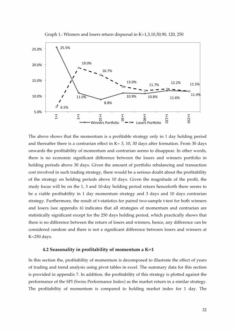
Interestingly, the momentum effect is only present in k=1 (1 day HPR) and afterwards the profitability of momentum shrinks and almost in all other holding periods, the losers yields a higher profit than the winners, therefore, a contrarian effect is observed in K=3,10, 30, 90 days after formation period. The following graphs demonstrates a dispersal in average return of losers and winners portfolios at 1 day holding period (K=1) between 1992 to 2011:

28 Critical two tail region of between -1.96 to 1.96

32

The above shows that the momentum is a profitable strategy only in 1 day holding period and thereafter there is a contrarian effect in K= 3, 10, 30 days after formation. From 30 days onwards the profitability of momentum and contrarian seems to disappear. In other words, there is no economic significant difference between the losers and winners portfolio in holding periods above 30 days. Given the amount of portfolio rebalancing and transaction cost involved in such trading strategy, there would be a serious doubt about the profitability of the strategy on holding periods above 10 days. Given the magnitude of the profit, the study focus will be on the 1, 3 and 10-day holding period return henceforth there seems to be a viable profitability in 1 day momentum strategy and 3 days and 10 days contrarian strategy. Furthermore, the result of t-statistics for paired two-sample t-test for both winners and losers (see appendix 6) indicates that all strategies of momentum and contrarian are statistically significant except for the 250 days holding period, which practically shows that there is no difference between the return of losers and winners, hence, any difference can be considered random and there is not a significant difference between losers and winners at K=250 days.

4.2 Seasonality in profitability of momentum a K=1

In this section the, profitability of momentum is decomposed to illustrate the effect of years of trading and trend analysis using pivot tables in excel. The summary data for this section is provided in appendix 7. In addition, the profitability of this strategy is plotted against the performance of the SPI (Swiss Performance Index) as the market return in a similar strategy. The profitability of momentum is compared to holding market index for 1 day. The

25.5%  

11.0%  8.8%  

10.9%   10.8%   11.6%  11.4%  

6.5%  

19.0%  

16.7%  

13.0%  11.7%   12.2%   11.5%  

5.0%  

10.0%  

15.0%  

20.0%  

25.0%  

t+1  

t+3  

t+10  

t+30  

t+90  

t+120  

t+250  

Graph 1.: Winners and losers return dispursal in K=1,3,10,30,90, 120, 250!

Winners  Por8olio   Losers  Por8olio  

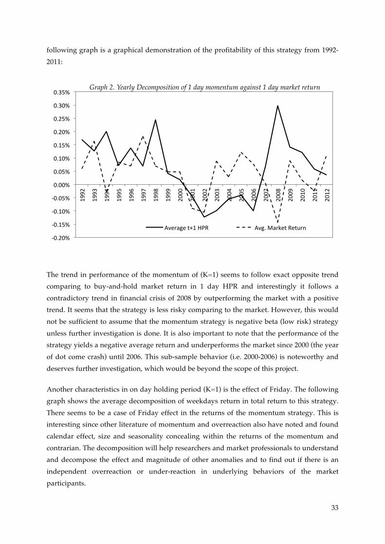
33

following graph is a graphical demonstration of the profitability of this strategy from 1992- 2011:

The trend in performance of the momentum of (K=1) seems to follow exact opposite trend comparing to buy-and-hold market return in 1 day HPR and interestingly it follows a contradictory trend in financial crisis of 2008 by outperforming the market with a positive trend. It seems that the strategy is less risky comparing to the market. However, this would not be sufficient to assume that the momentum strategy is negative beta (low risk) strategy unless further investigation is done. It is also important to note that the performance of the strategy yields a negative average return and underperforms the market since 2000 (the year of dot come crash) until 2006. This sub-sample behavior (i.e. 2000-2006) is noteworthy and deserves further investigation, which would be beyond the scope of this project.

Another characteristics in on day holding period (K=1) is the effect of Friday. The following graph shows the average decomposition of weekdays return in total return to this strategy. There seems to be a case of Friday effect in the returns of the momentum strategy. This is interesting since other literature of momentum and overreaction also have noted and found calendar effect, size and seasonality concealing within the returns of the momentum and contrarian. The decomposition will help researchers and market professionals to understand and decompose the effect and magnitude of other anomalies and to find out if there is an independent overreaction or under-reaction in underlying behaviors of the market participants.

-­‐0.20%  

-­‐0.15%  

-­‐0.10%  

-­‐0.05%  

0.00%  

0.05%  

0.10%  

0.15%  

0.20%  

0.25%  

0.30%  

0.35%  

1992  

1993  

1994  

1995  

1996  

1997  

1998  

1999  

2000  

2001  

2002  

2003  

2004  

2005  

2006  

2007  

2008  

2009  

2010  

2011  

2012  

Graph 2. Yearly Decomposition of 1 day momentum against 1 day market return !

Average  t+1  HPR   Avg.  Market  Return  

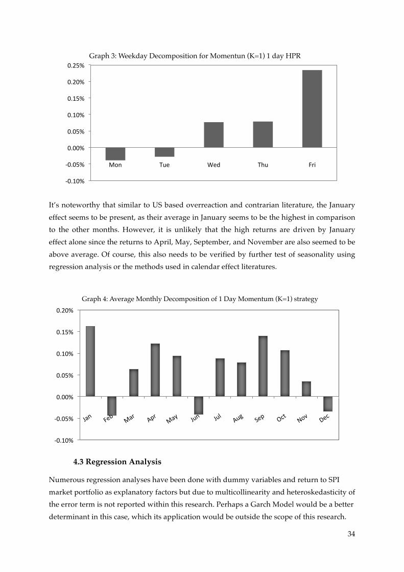
34

It’s noteworthy that similar to US based overreaction and contrarian literature, the January effect seems to be present, as their average in January seems to be the highest in comparison to the other months. However, it is unlikely that the high returns are driven by January effect alone since the returns to April, May, September, and November are also seemed to be above average. Of course, this also needs to be verified by further test of seasonality using regression analysis or the methods used in calendar effect literatures.

4.3 Regression Analysis

Numerous regression analyses have been done with dummy variables and return to SPI market portfolio as explanatory factors but due to multicollinearity and heteroskedasticity of the error term is not reported within this research. Perhaps a Garch Model would be a better determinant in this case, which its application would be outside the scope of this research.

-­‐0.10%  

-­‐0.05%  

0.00%  

0.05%  

0.10%  

0.15%  

0.20%  

0.25%  

Mon   Tue   Wed   Thu   Fri  

Graph 3: Weekday Decomposition for Momentun (K=1) 1 day HPR!

-­‐0.10%  

-­‐0.05%  

0.00%  

0.05%  

0.10%  

0.15%  

0.20%  

Graph 4: Average Monthly Decomposition of 1 Day Momentum (K=1) strategy!

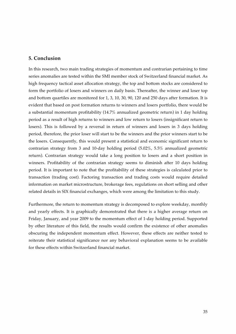
35

5. Conclusion

In this research, two main trading strategies of momentum and contrarian pertaining to time series anomalies are tested within the SMI member stock of Switzerland financial market. As high frequency tactical asset allocation strategy, the top and bottom stocks are considered to form the portfolio of losers and winners on daily basis. Thereafter, the winner and loser top and bottom quartiles are monitored for 1, 3, 10, 30, 90, 120 and 250 days after formation. It is evident that based on post formation returns to winners and losers portfolio, there would be a substantial momentum profitability (14.7% annualized geometric return) in 1 day holding period as a result of high returns to winners and low return to losers (insignificant return to losers). This is followed by a reversal in return of winners and losers in 3 days holding period, therefore, the prior loser will start to be the winners and the prior winners start to be the losers. Consequently, this would present a statistical and economic significant return to contrarian strategy from 3 and 10-day holding period (5.02%, 5.5% annualized geometric return). Contrarian strategy would take a long position to losers and a short position in winners. Profitability of the contrarian strategy seems to diminish after 10 days holding period. It is important to note that the profitability of these strategies is calculated prior to transaction (trading cost). Factoring transaction and trading costs would require detailed information on market microstructure, brokerage fees, regulations on short selling and other related details in SIX financial exchanges, which were among the limitation to this study.

Furthermore, the return to momentum strategy is decomposed to explore weekday, monthly and yearly effects. It is graphically demonstrated that there is a higher average return on Friday, January, and year 2009 to the momentum effect of 1-day holding period. Supported by other literature of this field, the results would confirm the existence of other anomalies obscuring the independent momentum effect. However, these effects are neither tested to reiterate their statistical significance nor any behavioral explanation seems to be available for these effects within Switzerland financial market.

36

6. References (bibliography)

N. Ali, et al. (2009a). ‘Does Bursa Malaysia Overreact?’. International Research Journal of Finance and Economics . N. Ali, et al. (2009b). ‘Stock Overreaction and Financial Bubbles: Evidence from Malaysia’. Journal of Money, Investment and Banking (11). K. Assoe & O. Sy (2009). ‘Profitability of the Short-Run Contrarian Strategy in Canadian Stock Markets’. Canadian Journal of Administrative Sciences / Revue Canadienne des Sciences de l’Administration 20(4):311–319. R. Ball & S. P. Kothari (1989). ‘Nonstationary expected returns’. Journal of Financial Economics 25(1):51–74. R. Ball, et al. (1995). ‘Problems in measuring portfolio performance An application to contrarian investment strategies’. Journal of Financial Economics 38(1):79–107. K. C. Brown, et al. (1988). ‘Risk Aversion, uncertain information, and market efficiency’. Journal of Financial Economics 22:355–389. J. Y. Campbell, et al. (1997). The econometrics of financial markets. Princeton University Press. K. C. Chan (1988). ‘On the Contrarian Investment Strategy’. The Journal of Business 61(2):147–163. K. C. Chan, et al. (1996). ‘Momentum Strategies’. The Journal of Finance 5. C. R. Chen & D. A. Sauer (1997). ‘Is Stock Market Overreaction Persistent Over Time?’. Journal of Business Finance & Accounting 24(1):51–66. N. Chopra, et al. (1992). ‘Measuring abnormal performance’. Journal of Financial Economics 31(2):235–268. T. Chordia & L. Shivakumar (2001a). ‘Earnings, Business Cycle And Stock Returns’. Social Science Research Network Working Paper Series . T. Chordia & L. Shivakumar (2001b). ‘Momentum, Business Cycle and Time Varying Expected Returns’. Social Science Research Network Working Paper Series . A. Clare & S. Thomas (1995). ‘THE OVERREACTION HYPOTHESIS AND THE UK STOCKMARKET’. Journal of Business Finance & Accounting 22(7):961–973. J. Conrad & G. Kaul (1998). ‘An Anatomy of Trading Strategies’. The Review of Financial Studies 11(3):489–519. K. Daniel, et al. (1998). ‘Investor Psychology and Security Market under- and Overreactions’. The Journal of Finance 53(6):1839–1885. W. F. M. De Bondt & R. Thaler (1985). ‘Does the Stock Market Overreact?’. The Journal of Finance 40(3):793–805. J. B. De Long;, et al. (1990). ‘Noise Trader Risk in Financial Markets’. The Journal of Political Economy 98(4):703–738.

37

W. F. M. DeBondt & R. H. Thaler (1986). ‘Further Evidence on Investor Overreaction and Stock Market Seasonality’. The Journal of Finance 42(3):557–581. M. Dubois & J.-F. Bacmann (1998). ‘Contrarian Strategies and Cross-Autocorrelations in Stock Returns: Evidence From France’. Social Science Research Network Working Paper Series . R. B. Durand, et al. (2006). ‘Momentum in Australia—A Note’. Australian Journal of Management 31(2):355–364. E. F. Fama (1970), ‘Efficient Capital Markets: A Review of Theory and Empirical Work’. Journal of Finance:25(2):383-417 E. F. Fama (1997). ‘Market Efficiency, Long-Term Returns, and Behavioral Finance’. Social Science Research Network Working Paper Series . B. D. Grundy & J. S. Martin (2001). ‘Understanding the nature of the risks and the source of the rewards to momentum investing’. Review of Financial Studies 14(1):29–78. S. Hurn & V. Pavlov (2003). ‘Momentum in Australian Stock Returns’. Australian Journal of Management 28(2):141–155. N. Jagadeesh (1990). ‘Evidence of predictable behavior of security return’. The journal of finance 45(3):881–98. N. Jegadeesh & S. Titman (1993). ‘Returns to Buying Winners and Selling Losers: Implications for Stock Market Efficiency’. The Journal of Finance 48(1):65–91. N. Jegadeesh & S. Titman (1999). ‘Profitability of Momentum Strategies: An Evaluation of Alternative Explanations’. Social Science Research Network Working Paper Series . M. C. Jensen (1967). ‘The Performance of Mutual Funds in the Period 1945-1964’. Journal of Finance 23(2):389–416. D. A. Lesmond, et al. (2003). ‘The Illusory Nature of Momentum Profits’. Social Science Research Network Working Paper Series . J. Lewellen (2002). ‘Momentum and Autocorrelation in Stock Returns’. Review of Financial Studies 15(2):533–564. A. W. Lo & A. C. MacKinlay (1990). ‘When are contrarian profits due to stock market overreaction?’. Review of Financial Studies 3(2):175–205. T. H. McInish, et al. (2008). ‘Short-horizon contrarian and momentum strategies in Asian markets: An integrated analysis’. International Review of Financial Analysis 17(2):312–329. M. G. McMillan & C. Institute. (2011). Investments workbook : principles of portfolio and equity analysis. Wiley. V. Ramiah, et al. (2011). ‘Hot and Cold Strategies: Australian Evidence’. Review of Pacific Basin Financial Markets and Policies 14(02):271+. D. M. Rey & M. M. Schmid (2004). ‘Feasible Momentum Strategies - Evidence from the Swiss Stock Market’. Social Science Research Network Working Paper Series .

38

K. G. Rouwenhorst (2004). ‘International Momentum Strategies’. Social Science Research Network Working Paper Series . S. Yochanan (2002). ‘The Behavior of Secondary European Stock. Markets to Positive and Negative Shocks’. International Journal of Business 7(2).

P. Zarowin (1990). ‘Size, Seasonality, and Stock Market Overreaction’. The Journal of Financial and Quantitative Analysis 25(1):113–125.

39

7. List of tables

Table 1- Sampling of Observed Pricing Anomalies

Time Series Cross-Sectional Other January effect Size effect Closed-end fund discount Day-of-the-week effect Value effect Earning surprise Weekend effect Book-to-market ration Initial public offerings Turn-of-the-month effect Value line enigma Distressed securities effect Holiday effect Stock split Time-of-day effect Super bowl Momentum Overreaction Source: McMillan et al. (2011)

Table 2- SMI Members Companies

SMI member companies 1 ABB 2 ACTELION 3 ADECCO 4 CREDIT SUISSE GROUP 5 GIVAUDAN 6 HOLCIM 7 JULIUS 8 NESTLE 9 NOVARTIS 10 RICHEMONT 11 ROCHE HOLDING 12 SGS 13 THE SWATCH GROUP 14 SWISS 15 SWISSCOM 16 SYNGENTA 17 SYNTHES 18 TRANSOCEAN (SWX) 19 UBS 20 ZURICH INSURANCE GROUP

   

40

8. Appendices

Appendix 1. Swiss market graphic representation of different indices

source: http://www.six-swiss-exchange.com/index_info/online/share_indices/smi/smifamily_factsheet_en.pdf

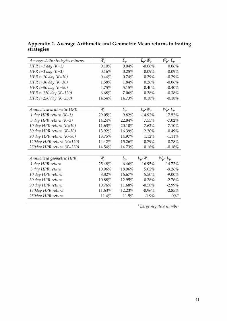
41

Appendix 2- Average Arithmetic and Geometric Mean returns to trading strategies

Average daily strategies returns !! !! !!-!! !!- !! HPR t+1 day (K=1) 0.10% 0.04% -0.06% 0.06% HPR t+3 day (K=3) 0.16% 0.25% 0.09% -0.09% HPR t+10 day (K=10) 0.44% 0.74% 0.29% -0.29% HPR t+30 day (K=30) 1.58% 1.84% 0.26% -0.06% HPR t+90 day (K=90) 4.75% 5.15% 0.40% -0.40% HPR t+120 day (K=120) 6.68% 7.06% 0.38% -0.38% HPR t+250 day (K=250) 14.54% 14.73% 0.18% -0.18%

Annualized arithmetic HPR !! !! !!-!! !!- !! 1 day HPR return (K=1) 29.05% 9.82% -14.92% 17.52% 3 day HPR return (K=3) 14.24% 22.84% 7.55% -7.02% 10 day HPR return (K=10) 11.63% 20.10% 7.62% -7.10% 30 day HPR return (K=30) 13.92% 16.39% 2.20% -0.49% 90 day HPR return (K=90) 13.75% 14.97% 1.12% -1.11% 120day HPR return (K=120) 14.42% 15.26% 0.79% -0.78% 250day HPR return (K=250) 14.54% 14.73% 0.18% -0.18%

Annualized geometric HPR !! !! !!-!! !!- !! 1 day HPR return 25.48% 6.46% -16.95% 14.72% 3 day HPR return 10.96% 18.96% 5.02% -9.26% 10 day HPR return 8.82% 16.67% 5.50% -9.00% 30 day HPR return 10.88% 12.95% 0.28% -2.76% 90 day HPR return 10.76% 11.68% -0.58% -2.99% 120day HPR return 11.63% 12.23% -0.96% -2.85% 250day HPR return 11.4% 11.5% -1.9% 0%*

* Large negative number

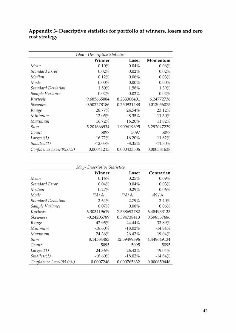
42

Appendix 3- Descriptive statistics for portfolio of winners, losers and zero cost strategy

       1day - Descriptive Statistics

Winner Loser Momentum

Mean 0.10% 0.04% 0.06% Standard Error 0.02% 0.02% 0.02% Median 0.12% 0.06% 0.03% Mode 0.00% 0.00% 0.00% Standard Deviation 1.50% 1.58% 1.39% Sample Variance 0.02% 0.02% 0.02% Kurtosis 9.685665084 8.233308401 6.24772736 Skewness 0.502278186 0.250931288 0.012056075 Range 28.77% 24.54% 23.12% Minimum -12.05% -8.35% -11.30% Maximum 16.72% 16.20% 11.82% Sum 5.201666934 1.909619695 3.292047239 Count 5097 5097 5097 Largest(1) 16.72% 16.20% 11.82% Smallest(1) -12.05% -8.35% -11.30% Confidence Level(95.0%) 0.00041215 0.000433506 0.000381638

3day- Descriptive Statistics

Winner Loser Contrarian

Mean 0.16% 0.25% 0.09% Standard Error 0.04% 0.04% 0.03% Median 0.27% 0.29% 0.06% Mode #N/A #N/A #N/A Standard Deviation 2.64% 2.79% 2.40% Sample Variance 0.07% 0.08% 0.06% Kurtosis 6.303419619 7.538692782 6.484933123 Skewness -0.24205789 0.394738413 0.598557686 Range 42.95% 44.44% 33.89% Minimum -18.60% -18.02% -14.84% Maximum 24.36% 26.42% 19.04% Sum 8.14534483 12.59499396 4.449649134 Count 5095 5095 5095 Largest(1) 24.36% 26.42% 19.04% Smallest(1) -18.60% -18.02% -14.84% Confidence Level(95.0%) 0.0007246 0.000765632 0.000659446

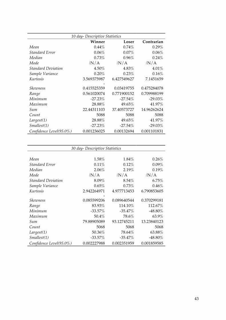
43

10 day- Descriptive Statistics

Winner Loser Contrarian

Mean 0.44% 0.74% 0.29% Standard Error 0.06% 0.07% 0.06% Median 0.73% 0.96% 0.24% Mode #N/A #N/A #N/A Standard Deviation 4.50% 4.83% 4.01% Sample Variance 0.20% 0.23% 0.16% Kurtosis 3.569375987 6.427549627 7.1451659

Skewness -

0.415525359 0.03419755 0.475284078 Range 0.561020074 0.771900152 0.709988199 Minimum -27.23% -27.54% -29.03% Maximum 28.88% 49.65% 41.97% Sum 22.44311103 37.40573727 14.96262624 Count 5088 5088 5088 Largest(1) 28.88% 49.65% 41.97% Smallest(1) -27.23% -27.54% -29.03% Confidence Level(95.0%) 0.001236025 0.00132694 0.001101831

30 day- Descriptive Statistics

Mean 1.58% 1.84% 0.26% Standard Error 0.11% 0.12% 0.09% Median 2.06% 2.19% 0.19% Mode #N/A #N/A #N/A Standard Deviation 8.09% 8.54% 6.75% Sample Variance 0.65% 0.73% 0.46% Kurtosis 2.942264971 4.977713453 6.790853605

Skewness -

0.085599206 0.089640544 0.370299181 Range 83.93% 114.10% 112.67% Minimum -33.57% -35.47% -48.80% Maximum 50.4% 78.6% 63.9% Sum 79.88905089 93.12745211 13.23840123 Count 5068 5068 5068 Largest(1) 50.36% 78.64% 63.88% Smallest(1) -33.57% -35.47% -48.80% Confidence Level(95.0%) 0.002227988 0.002351959 0.001859585

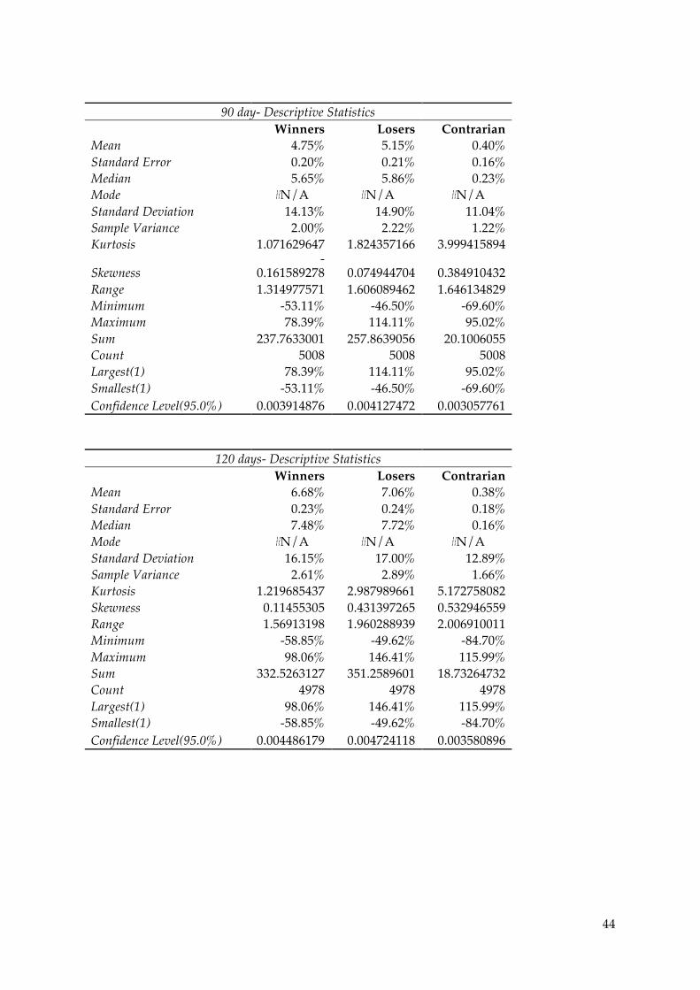
44

90 day- Descriptive Statistics

Winners Losers Contrarian

Mean 4.75% 5.15% 0.40% Standard Error 0.20% 0.21% 0.16% Median 5.65% 5.86% 0.23% Mode #N/A #N/A #N/A Standard Deviation 14.13% 14.90% 11.04% Sample Variance 2.00% 2.22% 1.22% Kurtosis 1.071629647 1.824357166 3.999415894

Skewness -

0.161589278 0.074944704 0.384910432 Range 1.314977571 1.606089462 1.646134829 Minimum -53.11% -46.50% -69.60% Maximum 78.39% 114.11% 95.02% Sum 237.7633001 257.8639056 20.1006055 Count 5008 5008 5008 Largest(1) 78.39% 114.11% 95.02% Smallest(1) -53.11% -46.50% -69.60% Confidence Level(95.0%) 0.003914876 0.004127472 0.003057761

120 days- Descriptive Statistics

Winners Losers Contrarian

Mean 6.68% 7.06% 0.38% Standard Error 0.23% 0.24% 0.18% Median 7.48% 7.72% 0.16% Mode #N/A #N/A #N/A Standard Deviation 16.15% 17.00% 12.89% Sample Variance 2.61% 2.89% 1.66% Kurtosis 1.219685437 2.987989661 5.172758082 Skewness 0.11455305 0.431397265 0.532946559 Range 1.56913198 1.960288939 2.006910011 Minimum -58.85% -49.62% -84.70% Maximum 98.06% 146.41% 115.99% Sum 332.5263127 351.2589601 18.73264732 Count 4978 4978 4978 Largest(1) 98.06% 146.41% 115.99% Smallest(1) -58.85% -49.62% -84.70% Confidence Level(95.0%) 0.004486179 0.004724118 0.003580896

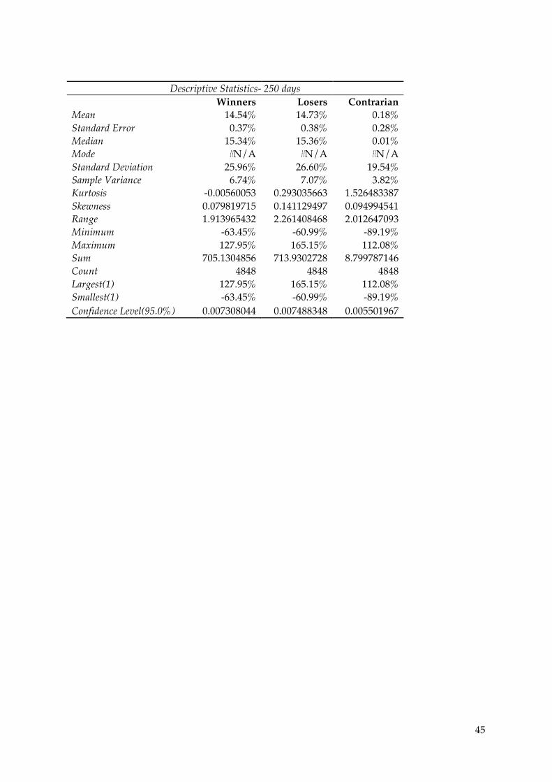
45

Descriptive Statistics- 250 days

Winners Losers Contrarian

Mean 14.54% 14.73% 0.18% Standard Error 0.37% 0.38% 0.28% Median 15.34% 15.36% 0.01% Mode #N/A #N/A #N/A Standard Deviation 25.96% 26.60% 19.54% Sample Variance 6.74% 7.07% 3.82% Kurtosis -0.00560053 0.293035663 1.526483387 Skewness 0.079819715 0.141129497 0.094994541 Range 1.913965432 2.261408468 2.012647093 Minimum -63.45% -60.99% -89.19% Maximum 127.95% 165.15% 112.08% Sum 705.1304856 713.9302728 8.799787146 Count 4848 4848 4848 Largest(1) 127.95% 165.15% 112.08% Smallest(1) -63.45% -60.99% -89.19% Confidence Level(95.0%) 0.007308044 0.007488348 0.005501967

46

Appendix 5 –Test of significance for mean returns of losers and winners in difference holding periods (t-test for hypothesized mean of zero)

Winner (1 Day HPR)

Losers (1 Day HPR)

Data Data Null Hypothesis m= 0 Null Hypothesis m= 0 Level of Significance 0.05 Level of Significance 0.05 Sample Size 5097 Sample Size 5097 Sample Mean 0.001020535 Sample Mean 0.000374656 Sample Standard Deviation 0.015009324 Sample Standard Deviation 0.015787051

Intermediate Calculations Intermediate Calculations Standard Error of the Mean 0.000210234 Standard Error of the Mean 0.000221128 Degrees of Freedom 5096 Degrees of Freedom 5096 t Test Statistic 4.854271768 t Test Statistic 1.694293207

Two-Tailed Test Two-Tailed Test Lower Critical Value -1.96042961 Lower Critical Value -1.96042961 Upper Critical Value 1.96042961 Upper Critical Value 1.96042961 p-Value 1.24438E-06 p-Value 0.090270684

Do not reject the null hypothesis Do not reject the null hypothesis

Winners (3day HPR)

Losers (3 Day HPR)

Data Data Null Hypothesis m= 0 Null Hypothesis m= 0 Level of Significance 0.05 Level of Significance 0.05 Sample Size 5095 Sample Size 5095 Sample Mean 0.001598694 Sample Mean 0.00247203 Sample Standard Deviation 0.026382695 Sample Standard Deviation 0.02787668

Intermediate Calculations Intermediate Calculations Standard Error of the Mean 0.000369613 Standard Error of the Mean 0.000390543 Degrees of Freedom 5094 Degrees of Freedom 5094 t Test Statistic 4.325319777 t Test Statistic 6.329724625

Two-Tailed Test Two-Tailed Test Lower Critical Value -1.960429792 Lower Critical Value -1.960429792 Upper Critical Value 1.960429792 Upper Critical Value 1.960429792 p-Value 1.55222E-05 p-Value 2.66653E-10

Reject the null hypothesis Reject the null hypothesis

47

Winners (10 Day HPR)

Losers (10 Day HPR)

Data Data Null Hypothesis m= 0 Null Hypothesis m= 0 Level of Significance 0.05 Level of Significance 0.05 Sample Size 5088 Sample Size 5088 Sample Mean 0.44% Sample Mean 0.007351757 Sample Standard Deviation 0.044972748 Sample Standard Deviation 0.048280666

Intermediate Calculations Intermediate Calculations Standard Error of the Mean 0.000630487 Standard Error of the Mean 0.000676861 Degrees of Freedom 5087 Degrees of Freedom 5087 t Test Statistic 6.996165555 t Test Statistic 10.86154028

Two-Tailed Test Two-Tailed Test Lower Critical Value -1.960430434 Lower Critical Value -1.960430434 Upper Critical Value 1.960430434 Upper Critical Value 1.960430434 p-Value 2.97117E-12 p-Value 3.48668E-27

Reject the null hypothesis Reject the null hypothesis

Winners (30 Day HPR)

Losers (30 day HPR)

Data Data Null Hypothesis m= 0 Null Hypothesis m= 0 Level of Significance 0.05 Level of Significance 0.05 Sample Size 5068 Sample Size 5068 Sample Mean 0.015763428 Sample Mean 0.018375583 Sample Standard Deviation 0.080905749 Sample Standard Deviation 0.085407539

Intermediate Calculations Intermediate Calculations Standard Error of the Mean 0.001136478 Standard Error of the Mean 0.001199714 Degrees of Freedom 5067 Degrees of Freedom 5067 t Test Statistic 13.87041885 t Test Statistic 15.3166297

Two-Tailed Test Two-Tailed Test Lower Critical Value -1.960432275 Lower Critical Value -1.960432275 Upper Critical Value 1.960432275 Upper Critical Value 1.960432275 p-Value 5.78953E-43 p-Value 8.43954E-52

Reject the null hypothesis Reject the null hypothesis

48

Winners (90 Day HPR)

Losers (90 Day HPR)

Data Data Null Hypothesis m= 0 Null Hypothesis m= 0 Level of Significance 0.05 Level of Significance 0.05 Sample Size 5008 Sample Size 5008 Sample Mean 0.047476697 Sample Mean 0.051490396 Sample Standard Deviation 0.141317868 Sample Standard Deviation 0.148992101

Intermediate Calculations Intermediate Calculations Standard Error of the Mean 0.00199694 Standard Error of the Mean 0.002105383 Degrees of Freedom 5007 Degrees of Freedom 5007 t Test Statistic 23.7747294 t Test Statistic 24.45654766

Two-Tailed Test Two-Tailed Test Lower Critical Value -1.960437888 Lower Critical Value -1.960437888 Upper Critical Value 1.960437888 Upper Critical Value 1.960437888 p-Value 1.8012E-118 p-Value 7.0298E-125

Reject the null hypothesis Reject the null hypothesis

Winners (120 Day HPR)

Losers (120 Day HPR)

Data Data Null Hypothesis m= 0 Null Hypothesis m= 0 Level of Significance 0.05 Level of Significance 0.05 Sample Size 4978 Sample Size 4978 Sample Mean 6.68% Sample Mean 7.06% Sample Standard Deviation 0.161454583 Sample Standard Deviation 0.170017846

Intermediate Calculations Intermediate Calculations Standard Error of the Mean 0.002288353 Standard Error of the Mean 0.002409723 Degrees of Freedom 4977 Degrees of Freedom 4977 t Test Statistic 29.19094753 t Test Statistic 29.28231825

Two-Tailed Test Two-Tailed Test Lower Critical Value -1.960440745 Lower Critical Value -1.960440745 Upper Critical Value 1.960440745 Upper Critical Value 1.960440745 p-Value 4.7097E-173 p-Value 4.8053E-174

Reject the null hypothesis Reject the null hypothesis

49

Winners (250 Day HPR)

Losers (250 Day)

Data Data Null Hypothesis m= 0 Null Hypothesis m= 0 Level of Significance 0.05 Level of Significance 0.05 Sample Size 4848 Sample Size 4848 Sample Mean 14.54% Sample Mean 14.73% Sample Standard Deviation 0.259552933 Sample Standard Deviation 0.2659566

Intermediate Calculations Intermediate Calculations Standard Error of the Mean 0.003727732 Standard Error of the Mean 0.003819702 Degrees of Freedom 4847 Degrees of Freedom 4847 t Test Statistic 39.01775214 t Test Statistic 38.55349201

Two-Tailed Test Two-Tailed Test Lower Critical Value -1.960453536 Lower Critical Value -1.960453536 Upper Critical Value 1.960453536 Upper Critical Value 1.960453536 p-Value 7.6429E-290 p-Value 7.1636E-284

Reject the null hypothesis Reject the null hypothesis

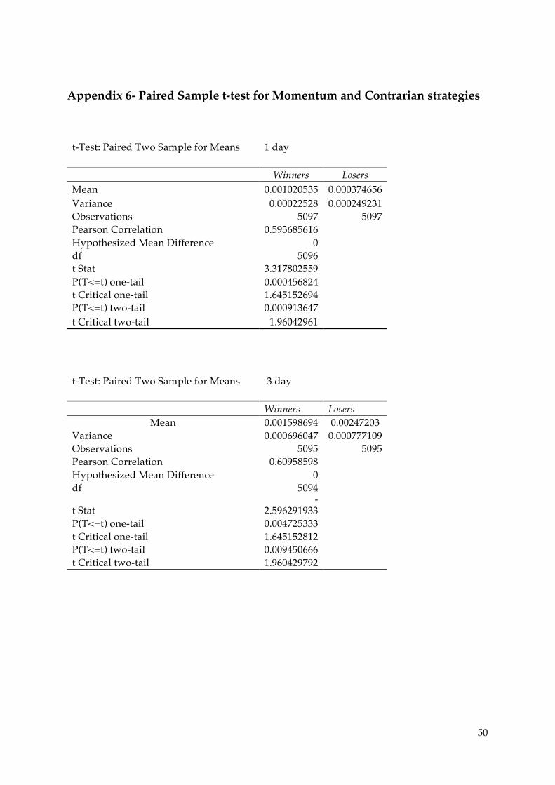
50

Appendix 6- Paired Sample t-test for Momentum and Contrarian strategies

t-Test: Paired Two Sample for Means 1 day

Winners Losers Mean 0.001020535 0.000374656 Variance 0.00022528 0.000249231 Observations 5097 5097 Pearson Correlation 0.593685616 Hypothesized Mean Difference 0 df 5096 t Stat 3.317802559 P(T<=t) one-tail 0.000456824 t Critical one-tail 1.645152694 P(T<=t) two-tail 0.000913647 t Critical two-tail 1.96042961 t-Test: Paired Two Sample for Means 3 day Winners Losers

Mean 0.001598694 0.00247203 Variance 0.000696047 0.000777109 Observations 5095 5095 Pearson Correlation 0.60958598 Hypothesized Mean Difference 0 df 5094

t Stat -

2.596291933 P(T<=t) one-tail 0.004725333 t Critical one-tail 1.645152812 P(T<=t) two-tail 0.009450666 t Critical two-tail 1.960429792

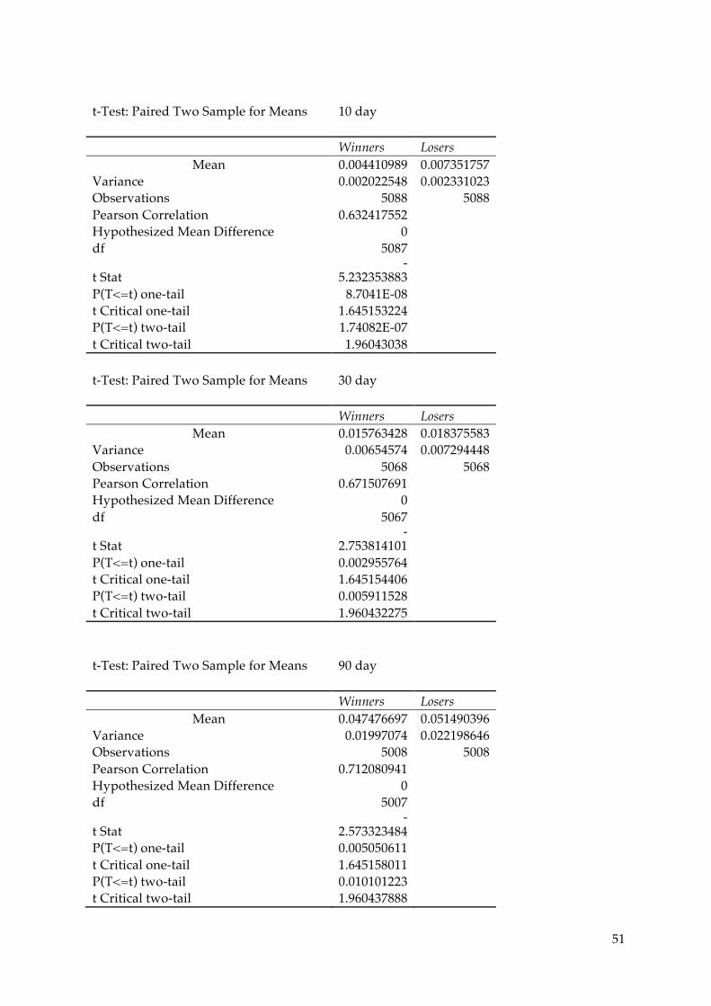
51

t-Test: Paired Two Sample for Means 10 day Winners Losers

Mean 0.004410989 0.007351757 Variance 0.002022548 0.002331023 Observations 5088 5088 Pearson Correlation 0.632417552 Hypothesized Mean Difference 0 df 5087

t Stat -

5.232353883 P(T<=t) one-tail 8.7041E-08 t Critical one-tail 1.645153224 P(T<=t) two-tail 1.74082E-07 t Critical two-tail 1.96043038 t-Test: Paired Two Sample for Means 30 day Winners Losers

Mean 0.015763428 0.018375583 Variance 0.00654574 0.007294448 Observations 5068 5068 Pearson Correlation 0.671507691 Hypothesized Mean Difference 0 df 5067

t Stat -

2.753814101 P(T<=t) one-tail 0.002955764 t Critical one-tail 1.645154406 P(T<=t) two-tail 0.005911528 t Critical two-tail 1.960432275 t-Test: Paired Two Sample for Means 90 day Winners Losers

Mean 0.047476697 0.051490396 Variance 0.01997074 0.022198646 Observations 5008 5008 Pearson Correlation 0.712080941 Hypothesized Mean Difference 0 df 5007

t Stat -

2.573323484 P(T<=t) one-tail 0.005050611 t Critical one-tail 1.645158011 P(T<=t) two-tail 0.010101223 t Critical two-tail 1.960437888

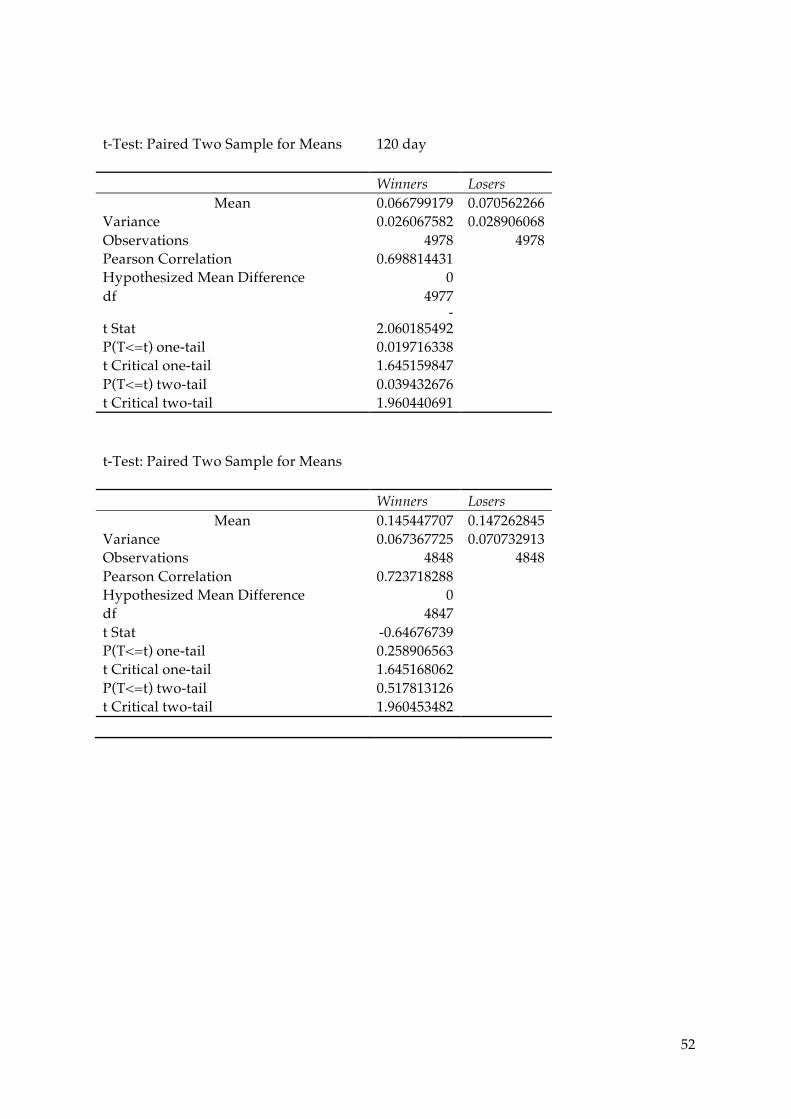
52

t-Test: Paired Two Sample for Means 120 day Winners Losers

Mean 0.066799179 0.070562266 Variance 0.026067582 0.028906068 Observations 4978 4978 Pearson Correlation 0.698814431 Hypothesized Mean Difference 0 df 4977

t Stat -

2.060185492 P(T<=t) one-tail 0.019716338 t Critical one-tail 1.645159847 P(T<=t) two-tail 0.039432676 t Critical two-tail 1.960440691 t-Test: Paired Two Sample for Means Winners Losers

Mean 0.145447707 0.147262845 Variance 0.067367725 0.070732913 Observations 4848 4848 Pearson Correlation 0.723718288 Hypothesized Mean Difference 0 df 4847 t Stat -0.64676739 P(T<=t) one-tail 0.258906563 t Critical one-tail 1.645168062 P(T<=t) two-tail 0.517813126 t Critical two-tail 1.960453482

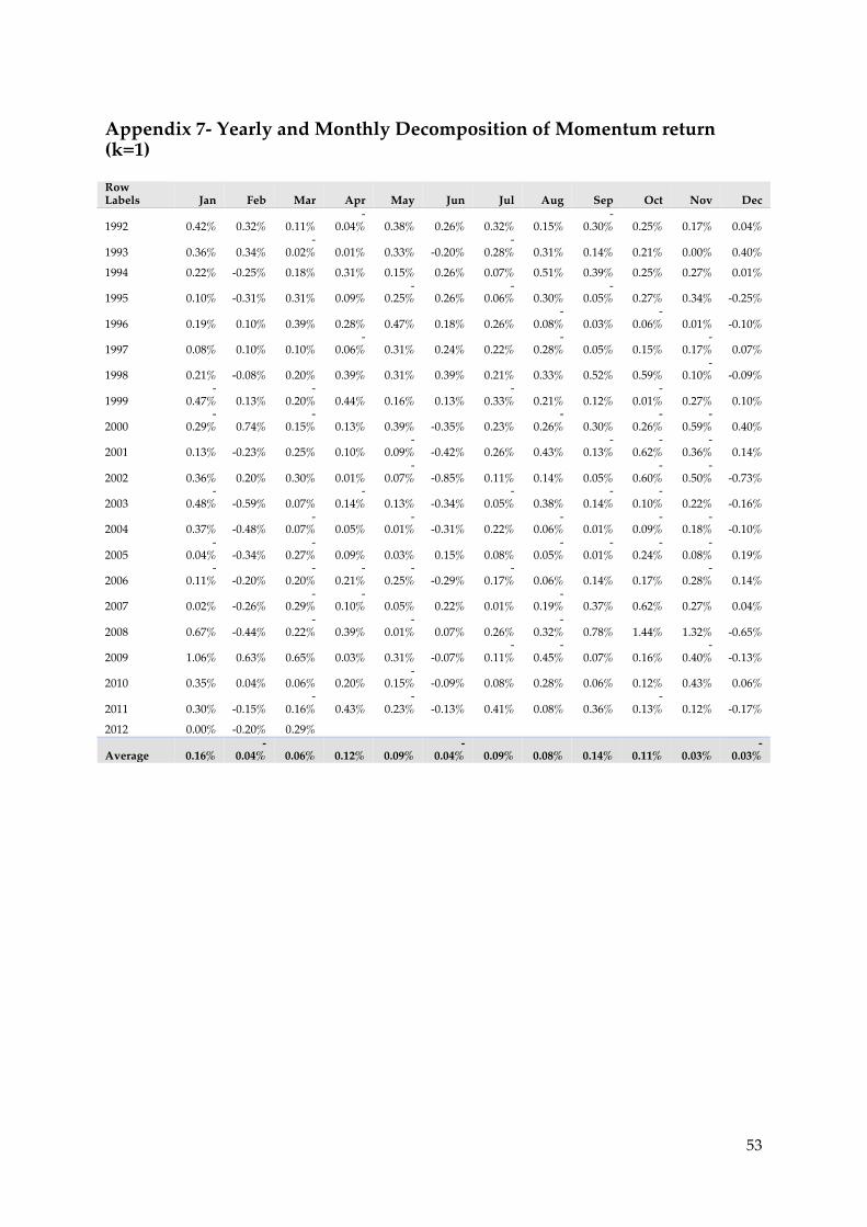
53

Appendix 7- Yearly and Monthly Decomposition of Momentum return (k=1)

Row Labels Jan Feb Mar Apr May Jun Jul Aug Sep Oct Nov Dec

1992 0.42% 0.32% 0.11% -

0.04% 0.38% 0.26% 0.32% 0.15% -

0.30% 0.25% 0.17% 0.04%

1993 0.36% 0.34% -

0.02% 0.01% 0.33% -0.20% -

0.28% 0.31% 0.14% 0.21% 0.00% 0.40% 1994 0.22% -0.25% 0.18% 0.31% 0.15% 0.26% 0.07% 0.51% 0.39% 0.25% 0.27% 0.01%

1995 0.10% -0.31% 0.31% 0.09% -

0.25% 0.26% -

0.06% 0.30% -

0.05% 0.27% 0.34% -0.25%

1996 0.19% 0.10% 0.39% 0.28% 0.47% 0.18% 0.26% -

0.08% 0.03% -

0.06% 0.01% -0.10%

1997 0.08% 0.10% 0.10% -

0.06% 0.31% 0.24% 0.22% -

0.28% 0.05% 0.15% -

0.17% 0.07%

1998 0.21% -0.08% 0.20% 0.39% 0.31% 0.39% 0.21% 0.33% 0.52% 0.59% -

0.10% -0.09%

1999 -

0.47% 0.13% -

0.20% 0.44% 0.16% 0.13% -

0.33% 0.21% 0.12% -

0.01% 0.27% 0.10%

2000 -

0.29% 0.74% -

0.15% 0.13% 0.39% -0.35% 0.23% -

0.26% 0.30% -

0.26% -

0.59% 0.40%

2001 0.13% -0.23% 0.25% 0.10% -

0.09% -0.42% 0.26% 0.43% -

0.13% -

0.62% -

0.36% 0.14%

2002 0.36% 0.20% 0.30% 0.01% -

0.07% -0.85% 0.11% 0.14% 0.05% -

0.60% -

0.50% -0.73%

2003 -

0.48% -0.59% 0.07% -

0.14% 0.13% -0.34% -

0.05% 0.38% -

0.14% -

0.10% 0.22% -0.16%

2004 0.37% -0.48% -

0.07% 0.05% -

0.01% -0.31% 0.22% -

0.06% 0.01% -

0.09% -

0.18% -0.10%

2005 -

0.04% -0.34% -

0.27% 0.09% 0.03% 0.15% 0.08% -

0.05% -

0.01% -

0.24% -

0.08% 0.19%

2006 -

0.11% -0.20% -

0.20% -

0.21% -

0.25% -0.29% -

0.17% 0.06% 0.14% 0.17% -

0.28% 0.14%

2007 0.02% -0.26% -

0.29% -

0.10% 0.05% 0.22% 0.01% -

0.19% 0.37% 0.62% 0.27% 0.04%

2008 0.67% -0.44% -

0.22% 0.39% -

0.01% 0.07% 0.26% -

0.32% 0.78% 1.44% 1.32% -0.65%

2009 1.06% 0.63% 0.65% 0.03% 0.31% -0.07% -

0.11% -

0.45% 0.07% 0.16% -

0.40% -0.13%

2010 0.35% 0.04% 0.06% 0.20% -

0.15% -0.09% 0.08% 0.28% 0.06% 0.12% 0.43% 0.06%

2011 0.30% -0.15% -

0.16% 0.43% -

0.23% -0.13% 0.41% 0.08% 0.36% -

0.13% 0.12% -0.17% 2012 0.00% -0.20% 0.29%

Average 0.16%

-0.04% 0.06% 0.12% 0.09%

-0.04% 0.09% 0.08% 0.14% 0.11% 0.03%

-0.03%

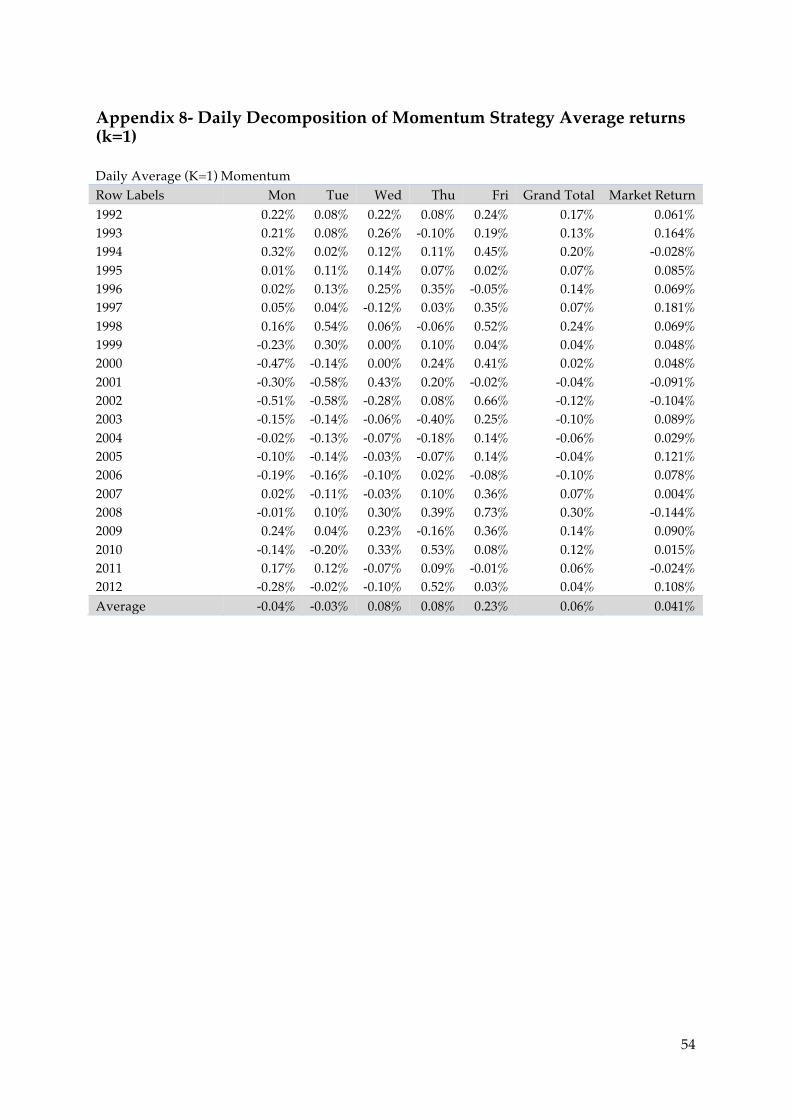
54

Appendix 8- Daily Decomposition of Momentum Strategy Average returns (k=1)

Daily Average (K=1) Momentum Row Labels Mon Tue Wed Thu Fri Grand Total Market Return

1992 0.22% 0.08% 0.22% 0.08% 0.24% 0.17% 0.061% 1993 0.21% 0.08% 0.26% -0.10% 0.19% 0.13% 0.164% 1994 0.32% 0.02% 0.12% 0.11% 0.45% 0.20% -0.028% 1995 0.01% 0.11% 0.14% 0.07% 0.02% 0.07% 0.085% 1996 0.02% 0.13% 0.25% 0.35% -0.05% 0.14% 0.069% 1997 0.05% 0.04% -0.12% 0.03% 0.35% 0.07% 0.181% 1998 0.16% 0.54% 0.06% -0.06% 0.52% 0.24% 0.069% 1999 -0.23% 0.30% 0.00% 0.10% 0.04% 0.04% 0.048% 2000 -0.47% -0.14% 0.00% 0.24% 0.41% 0.02% 0.048% 2001 -0.30% -0.58% 0.43% 0.20% -0.02% -0.04% -0.091% 2002 -0.51% -0.58% -0.28% 0.08% 0.66% -0.12% -0.104% 2003 -0.15% -0.14% -0.06% -0.40% 0.25% -0.10% 0.089% 2004 -0.02% -0.13% -0.07% -0.18% 0.14% -0.06% 0.029% 2005 -0.10% -0.14% -0.03% -0.07% 0.14% -0.04% 0.121% 2006 -0.19% -0.16% -0.10% 0.02% -0.08% -0.10% 0.078% 2007 0.02% -0.11% -0.03% 0.10% 0.36% 0.07% 0.004% 2008 -0.01% 0.10% 0.30% 0.39% 0.73% 0.30% -0.144% 2009 0.24% 0.04% 0.23% -0.16% 0.36% 0.14% 0.090% 2010 -0.14% -0.20% 0.33% 0.53% 0.08% 0.12% 0.015% 2011 0.17% 0.12% -0.07% 0.09% -0.01% 0.06% -0.024% 2012 -0.28% -0.02% -0.10% 0.52% 0.03% 0.04% 0.108% Average -0.04% -0.03% 0.08% 0.08% 0.23% 0.06% 0.041%