Embed Size (px)
DESCRIPTION
D.4.1-2 – Technical report Baseline scenario assumptions and model projections for selected target indicators Development of a Forecasting Framework and Scenarios to Support the EU Sustainable Development Strategy Baseline scenario assumptions and model projections for selected target indicators 4 BASELINE FORECASTING RESULTS FOR SELECTED INTERMEDIARY AND TARGET NODES 49
Citation preview

Project no.: 022793
FORESCENE
Development of a Forecasting Framework and Scenarios to Support the EU Sustainable
Development Strategy
Instrument: STREP
Thematic Priority 8.1: Policy-oriented research, scientific support to policies, integrating and
strengthening the European Research Area
D.4.1-2 – Technical report
Baseline scenario assumptions and model projections for selected target
indicators
Submission date: February 2009
Start date of project: 1/12/2005 Duration: 36 months
Organisation name of lead contractor for this deliverable:
Wuppertal Institute for Climate, Environment and Energy
Revision: final
Project co-funded by the European Commission within the Sixth Framework Programme (2002-2006)
Dissemination Level
PU Public X
PP Restricted to other programme participants (including the Commission Services)
RE Restricted to a group specified by the consortium (including the Commission Services)
CO Confidential, only for members of the consortium (including the Commission Services)

2

FORESCENE D.4.1-2 – Technical report
Baseline scenario assumptions and model projections for selected target parameters
3
Baseline scenario assumptions and model
projections for selected target indicators
Technical Report of Work Package 4
Stefan Bringezu, Mathieu Saurat
Roy Haines-Young, Alison Rollett
Mats Svensson
Wuppertal Institute for Climate, Environment and Energy
University of Nottingham, Centre for Environmental Management
Lund University, Centre for Sustainability Studies

4
FORESCENE D.4.1-2 – Technical report
Baseline scenario assumptions and model projections for selected target parameters
5
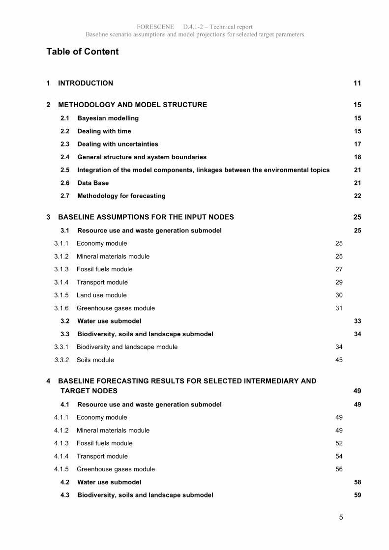
Table of Content
1 INTRODUCTION 11
2 METHODOLOGY AND MODEL STRUCTURE 15
2.1 Bayesian modelling 15
2.2 Dealing with time 15
2.3 Dealing with uncertainties 17
2.4 General structure and system boundaries 18
2.5 Integration of the model components, linkages between the environmental topics 21
2.6 Data Base 21
2.7 Methodology for forecasting 22
3 BASELINE ASSUMPTIONS FOR THE INPUT NODES 25
3.1 Resource use and waste generation submodel 25
3.1.1 Economy module 25
3.1.2 Mineral materials module 25
3.1.3 Fossil fuels module 27
3.1.4 Transport module 29
3.1.5 Land use module 30
3.1.6 Greenhouse gases module 31
3.2 Water use submodel 33
3.3 Biodiversity, soils and landscape submodel 34
3.3.1 Biodiversity and landscape module 34
3.3.2 Soils module 45
4 BASELINE FORECASTING RESULTS FOR SELECTED INTERMEDIARY AND
TARGET NODES 49
4.1 Resource use and waste generation submodel 49
4.1.1 Economy module 49
4.1.2 Mineral materials module 49
4.1.3 Fossil fuels module 52
4.1.4 Transport module 54
4.1.5 Greenhouse gases module 56
4.2 Water use submodel 58
4.3 Biodiversity, soils and landscape submodel 59

6
5 CONCLUSIONS 65
6 REFERENCES 67
7 APPENDIX 74
7.1 Conditional Probability Tables (CPTs) 74
7.2 Values for model input nodes of the biodiversity, soils and landscape submodel for
baseline scenarios 2000-2050 76
7.3 Definitions of forest land from Eurostat Forestry Statistics 2007 84

FORESCENE D.4.1-2 – Technical report
Baseline scenario assumptions and model projections for selected target parameters
7
List of Tables Table 1: Data base of the FORESCENE model prototype 22
Table 2: Mean material intensity values in EU-25 in 2000 26
Table 3: Mean values for hidden and indirect flow coefficients for EU-25 in 2000 and baseline
assumptions for the development until 2020 (mineral materials) 27
Table 4: Baseline assumption for gross inland energy consumption (GIC) (EC 2008) 28
Table 5: Mean values for hidden and indirect flow coefficients for EU-25 in 2000 and baseline
assumptions for the development until 2020 (fossil fuels and nuclear) 29
Table 6: Baseline assumptions for the transport module 29
Table 7: Baseline assumptions regarding biofuel consumption for the land use module 31
Table 8: Baseline assumptions regarding biofuel yields for the land use module (outside EU)
31
Table 9: GHG emissions improvements due to the use of biofuels compared to conventional
fuel (without land use change) 32
Table 10: Carbon debt 32
Table 11: Baseline assumptions for the water submodel 34
Table 12: Probability of percentage spend on AEP 35
Table 13: Probability of non-compliance with cross compliance regulations 35
Table 14: Certified forest area by region, 2005-2006 36
Table 15: Conservation status for mammal and plant species 2000-2005 and projections for
2010 40
Table 16: Projected probability of favourable and unfavourable conservation status for EU25
bird species (input node) 42
Table 17: Assumed increase in percentage of protected land area in the EU25 (input node)
45
Table 18: Projected share of gross domestic expenditure in R & D (% of GDP) (input node) 46
Table 19: Values for model input nodes of the biodiversity, soils and landscape submodel for
baseline scenarios 2000-2050 76
Table 20: Values for model input nodes of the biodiversity, soils and landscape submodel for
baseline scenarios 2000-2050 (Continued 1) 77
Table 21: Values for model input nodes of the biodiversity, soils and landscape submodel for
baseline scenarios 2000-2050 (Continued 2) 78
Table 22: Values for model input nodes of the biodiversity, soils and landscape submodel for
baseline scenarios 2000-2050 (Continued 3) 79
Table 23: Values for model input nodes of the biodiversity, soils and landscape submodel for
baseline scenarios 2000-2050 (Continued 4) 80

8
Table 24: Values for model input nodes of the biodiversity, soils and landscape submodel for
baseline scenarios 2000-2050 (Continued 5) 81
Table 25: List of nodes values with value used in place of normal distribution in baseline
model test 82

FORESCENE D.4.1-2 – Technical report
Baseline scenario assumptions and model projections for selected target parameters
9
List of Figures Figure 1: Socio-industrial metabolism and Driving Forces-Pressures-State-Impacts-
Response (DPSIR) framework in FORESCENE 13
Figure 2: The six questions of the FORESCENE framework 14
Figure 3: First option for dealing with time in Bayesian networks 16
Figure 4: Second option for dealing with time in Bayesian networks. 17
Figure 5: General overview of the structure of the FORESCENE model prototype. 18
Figure 6: Graphical representation of the Bayesian network for the FORESCENE meta
model 20
Figure 7: Forecasting method in the FORESCENE Bayesian network model prototype 24
Figure 8: Expected changes in habitat status from 2000-2050 under baseline projections
(input nodes) 38
Figure 9: Expected changes in habitat status from 2000-2050 under baseline projections
(continued) 39
Figure 10: Expected changes in species status from 2000-2050 under baseline projections
(input node) 41
Figure 11: Methodology for determination of EU25 conservation status for bird species 42
Figure 12: Current trends in EU mammal and bird populations 43
Figure 13: Projected probability of declining, stable, increasing or unknown trend in mammal
and bird populations (input nodes) 44
Figure 14: Projected probability that alien species are decreasing, stable or increasing over
the time period 2000-2050 (input node) 45
Figure 15: Projected greenhouse gas emissions for the period 2000-2050 (input node) 47
Figure 16: Assumed nutrient transfer efficiency for grassland and arable from 2000-2050
(input node) 47
Figure 17: Projected change in fertiliser use intensity for the baseline scenario 2000-2050
(input node) 48
Figure 18: Baseline modelling results for GDP 50
Figure 19: Baseline modelling results for TMR minerals 51
Figure 20: Baseline modelling results for the ratio foreign vs. domestic TMR minerals 51
Figure 21: Baseline modelling results for TMR fossil fuels 53
Figure 22: Baseline modelling results for the ratio foreign vs. domestic TMR fossil fuels 53
Figure 23: Baseline modelling results for biofuel consumption 54
Figure 24: Baseline modelling results for transport 55
Figure 25: Baseline modelling results for GHG emissions from fossil fuels 56

10
Figure 26: Baseline modelling results for GHG emissions savings from biofuel without land
use change 57
Figure 27: Baseline modelling results for GHG emissions savings from biofuel including land
use change 57
Figure 28: Baseline modelling results for total water withdrawals 58
Figure 29: Baseline modelling results for water balance 59
Figure 30: Modelled probability of aquatic, terrestrial and overall biodiversity status 60
Figure 31: Predicted model probability for soil erosion and soil carbon and the output node
soil quality 62
Figure 32: Predicted model probability for soil erosion and soil carbon and the output node
soil quality 63
Figure 33: Predicted model probability of species conservation status and trend in species
number 64
FORESCENE D.4.1-2 – Technical report
Baseline scenario assumptions and model projections for selected target parameters
11
1 Introduction
Since the Gothenburg summit in 2001, the implementation of the concept of sustainable
development has been a core challenge for policy making in the European Union. To
improve the basis for policy design, and also comply with the specific needs of ex-ante
impact assessments, there is a need for a forecasting framework to develop harmonised
middle and long-term baseline and alternative policy scenarios. In the context of the
Sustainable Development Strategy (European Commission 2001; Council of European
Union, 2006) the forecasting framework should allow to develop scenarios that can be used
for strategic policy preparation to better specify and disentangle the mutual relationships
between environmental, economic and social trends.
To be effective, policy development and appraisal needs to understand the key driving forces
and their cross-cutting linkages, which lead to increased pressure on different aspects of the
environment. Measures which are designed to solve single problems often risk shifting the
burden to other sectors, and they may be ineffective due to the complex interaction of
environmental effects. The need for policies to be based on a cross-cutting approach has
been highlighted in “The 2005 Review of the EU Sustainable Development Strategy: Initial
Stocktaking and future orientations” (COM(2005)37 final), as well as in the Commission’s
Communication on its Strategic Objectives 2005-2009 (COM (2005) 12). However, cross-
cutting driving forces which are relevant for various environmental and sustainability related
problems have not yet been analyzed in a systematic policy-oriented manner.
The FORESCENE project is an attempt to identify cross-cutting measures that are effective
and efficient, and which have the potential to mitigate several environmental problems at the
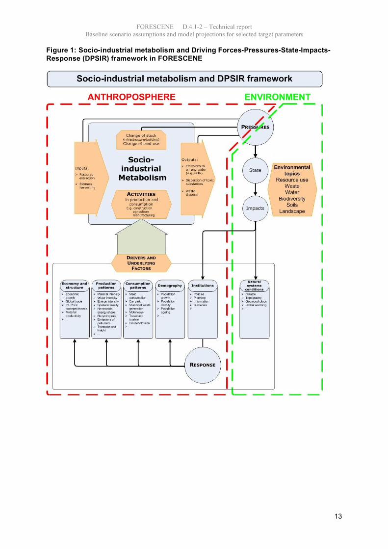
same time. As shown in Figure 1, three broad environmental themes are covered: ‘resource
use and waste generation’, ‘water’, and ‘biodiversity, soils and landscape’. The aim of the
project has been to capture the anthropogenic cross-cutting drivers that generate
environmental pressures and the inter-linkages between them, so that an integrated
forecasting framework could be constructed. It should, in turn, offer the possibility to test
alternative policy strategies against some baseline. To do so, the framework used in
FORESCENE was inspired and adapted from the backcasting methodology. As shown in
Figure 2, the project’s framework consists of six questions that were addressed during a
series of workshops. By applying the framework the project aimed to:
• determine cross-cutting (cross-thematic and cross-sectoral) driving forces for
environmental problems in the three targeted fields (relates to Question 1);
• define essential elements of sustainable development in the different topic areas,
particularly in the form of desired sustainability goals (relates to Question 2);
• describe cross-sectoral measures expected to exert a multi-beneficial impact over the
environmental fields considered, so that the sustainability goals identified can be
achieved (relates to Question 3); and,
• combine the scenario elements (driving forces, strategies, goals etc) into baseline
and alternative scenarios (relates to Questions 4 to 6).

12
The present report describes the approach taken to address Question 5 “What would happen
under business-as-usual conditions?” shown in Figure 2. As a result of Step 3 a model
prototype based on the Bayesian network methodology was developed. It consists of
interlinked sub-models featuring the environmental issues and cross-cutting drivers identified
in Step 1. The model prototype can then be used for forecasting exercises. The structure of
the model prototype, the methodological approach to Bayesian modelling, forecasting and
backcasting, and related issues are described in chapter 2.
Chapter 3 presents baseline assumptions made for the input nodes (driving and control
parameters) of the different modules of the model prototype. This lays the grounds for
modelling the baseline (or business-as-usual) scenario.
Using the forecasting methodology described in chapter 2, time series of key output variables
are modelled based on the assumptions made in chapter 3. The baseline projections for
selected intermediary and target parameters are presented in chapter 4. These baseline
modelling results will serve as a reference for comparison when alternative scenarios are
quantified in WP5.
Chapter 5 finally discusses the possibilities and perspectives to further develop the
framework and model. The ‘prototype’ baseline projections obtained in this workpackage also
offer perspectives for modelling alternative scenarios in WP5.
FORESCENE D.4.1-2 – Technical report
Baseline scenario assumptions and model projections for selected target parameters
13
Figure 1: Socio-industrial metabolism and Driving Forces-Pressures-State-Impacts-
Response (DPSIR) framework in FORESCENE

14
Figure 2: The six questions of the FORESCENE framework

FORESCENE D.4.1-2 – Technical report
Baseline scenario assumptions and model projections for selected target parameters
15
2 Methodology and model structure
2.1 Bayesian modelling
Bayesian networks (BNs) are an increasingly popular method applied to uncertain and
complex domains such as environmental modelling and management. They can be used as
or in combination with decision tools. BN models offer the possibility to incorporate
knowledge of different accuracies (e.g. absence/presence of an observation vs. quantitative
data from measurements) and from different sources (Marcot et al. 2001). Carefully elicited,
expert knowledge can be combined with empirical data, in a mathematically coherent
manner. Parameter values that come with uncertainties can be expressed as probability
distributions rather than average values. The higher the uncertainty, the wider is the
probability distribution. The end-point modelling results are also represented as probability
distributions which prevents overconfidence in single estimated values and allows for an
estimation of risks and uncertainties (Uusitalo 2007).
The Bayesian network approach to modelling presents, however, three main shortcomings
(Borsuk et al. 2004, Uusitalo 2007). First, BNs are acyclic graphs and therefore do not
support feedback loops (Jensen 2001). Second, and closely related shortcoming, is the
difficulty of modelling temporal dynamics in BNs. A possible workaround consists in using a
separate network for each time slice (Jensen 2001, Uusitalo 2007). This is however often
very tedious. The third difficulty associated with BN models is their limited ability to deal with
continuous data when used in compiled form. In such a form, the continuous variables and
parametric equations between variables need to be discretized over discrete domains
chosen by the user. This implies a trade-off as the discretization can only account for rough
characteristics of the original continuous distributions and relationships (Friedman and
Goldszmidt 1996). The problems inherent to the discretization of continuous variables can be
avoided by using the other major approach in Bayesian modelling beside Bayesian networks,
namely hierarchical simulation-based modelling (Uusitalo 2007, Gelman et al. 1995).
In the FORESCENE model prototype both branches of Bayesian modelling are implemented.
The network approach is used, for example, with the 'biodiversity, soils and landscape'
submodel that mainly consists of discrete variables. Once the submodel is compiled the BN
can provide instant responses to queries such as the modification of an input parameter. The
result is also directly visible in the graphical representation of the network.
The simulation-based approach is used for other modules of the model prototype that contain
mainly or exclusively continuous variables. The probability distributions of target parameters
are estimated by generating samples from these distributions by simulation (Gelman et al.
1995, Borsuk et al. 2003). The results, however, require some processing before they can be
shown. But, on the other hand, the least possible information is lost.
2.2 Dealing with time
It is important to note that the time dimension is not explicitly present in a Bayesian network
model. Using a collection of networks is an option to represent an evolution over time. Figure

16
3 shows how time dynamics is dealt with in FORESCENE, for some parts of the model
prototype (e.g. biodiversity and soils submodel). The networks of the time series differ from
one another by the input values of their marginal nodes, which correspond to initial input
values for given years. These inputs are calculated separately and for different scenarios.
The target nodes from each network then deliver output values for each year considered,
which can, in turn, be worked out into time series outside the networks.
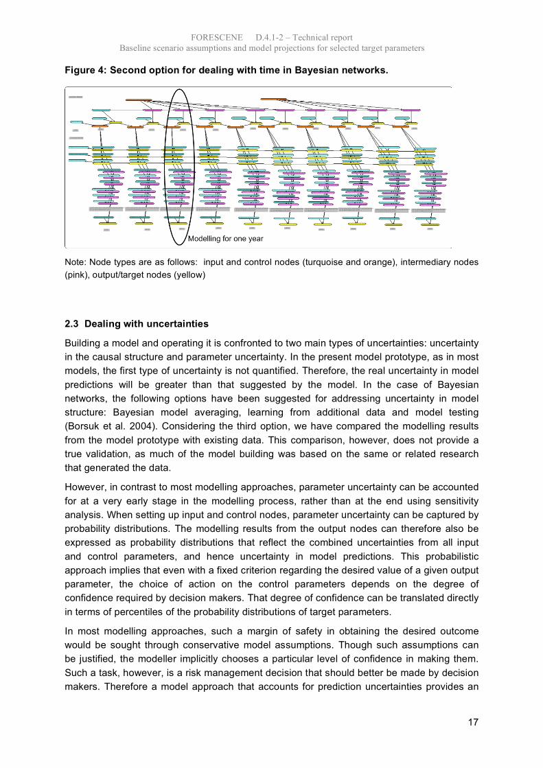
Another option consists in having the different years in one overall network (see Figure 4).
This option is adapted for networks used with simulation based modelling (see previous
section). It also facilitates the updating of input node values, for example for different
scenarios, as there is only one file to update. However, this option is to be reserved to
networks that are not too large and ramified.
Figure 3: First option for dealing with time in Bayesian networks
FORESCENE D.4.1-2 – Technical report
Baseline scenario assumptions and model projections for selected target parameters
17
Figure 4: Second option for dealing with time in Bayesian networks.
Note: Node types are as follows: input and control nodes (turquoise and orange), intermediary nodes
(pink), output/target nodes (yellow)
2.3 Dealing with uncertainties
Building a model and operating it is confronted to two main types of uncertainties: uncertainty
in the causal structure and parameter uncertainty. In the present model prototype, as in most
models, the first type of uncertainty is not quantified. Therefore, the real uncertainty in model
predictions will be greater than that suggested by the model. In the case of Bayesian
networks, the following options have been suggested for addressing uncertainty in model
structure: Bayesian model averaging, learning from additional data and model testing
(Borsuk et al. 2004). Considering the third option, we have compared the modelling results
from the model prototype with existing data. This comparison, however, does not provide a
true validation, as much of the model building was based on the same or related research
that generated the data.
However, in contrast to most modelling approaches, parameter uncertainty can be accounted
for at a very early stage in the modelling process, rather than at the end using sensitivity
analysis. When setting up input and control nodes, parameter uncertainty can be captured by
probability distributions. The modelling results from the output nodes can therefore also be
expressed as probability distributions that reflect the combined uncertainties from all input
and control parameters, and hence uncertainty in model predictions. This probabilistic
approach implies that even with a fixed criterion regarding the desired value of a given output
parameter, the choice of action on the control parameters depends on the degree of
confidence required by decision makers. That degree of confidence can be translated directly
in terms of percentiles of the probability distributions of target parameters.
In most modelling approaches, such a margin of safety in obtaining the desired outcome
would be sought through conservative model assumptions. Though such assumptions can
be justified, the modeller implicitly chooses a particular level of confidence in making them.
Such a task, however, is a risk management decision that should better be made by decision
makers. Therefore a model approach that accounts for prediction uncertainties provides an

18
explicit basis for choosing a decision criterion that includes a margin of safety. The size of
the margin, decided by decision makers, might be reduced by the decision makers
themselves if they settle for a lower degree of confidence, or by reducing prediction
uncertainty. The latter requires further data collection to reduce the uncertainty of input
parameters and of relationships between parameters. This, in turn, requires further
communication with stakeholders, experts and, eventually, decision makers. In that respect,
the explicit dealing with uncertainty of the Bayesian approach fits well in a heuristic
approach.
2.4 General structure and system boundaries
The general structure of the model prototype developed in the FORESCENE project is
shown in Figure 5. The geographical system boundaries are that of the EU-25 with regard to
the driving forces but the impacts on most of the environmental issues are considered at the
global level.
Figure 5: General overview of the structure of the FORESCENE model prototype.
Note: The components of the model considered beyond the EU-25 system borders are represented
with shadows.
More detailed, Figure 6 outlines the general structure of the model prototype, showing
variables and dependencies relevant for the selected environmental fields: ‘resource use and
waste generation’, ‘water’ and ‘biodiversity, landscape and soils’. The central part of the
figure represents the organising structure of the model, consisting of separately developed
modules. In the graphical representation of a Bayesian network, variables are depicted by
nodes, and a dependence between one variable and another is represented by an arrow.
The absence of an arrow between any two nodes implies the conditional independence.
Nodes can be either discrete (i.e. with a defined finite set of possible values called states) or
continuous (i.e. can take in a value between any other two values). The ‘sub-models’ are the
component parts of the model prototype, covering one of the three environmental topics, and
‘modules’ are component parts within a sub-model.
The following sub-models and modules are shown in Figure 6:

FORESCENE D.4.1-2 – Technical report
Baseline scenario assumptions and model projections for selected target parameters
19
• Economy
• Mineral materials
• Fossil fuels
• Biofuels
• GHG emissions
• Agricultural land use
• Water
• Biodiversity and soils
Some modules have been or could be developed in more complex versions, in order, for
example, to further differentiate and parametrise mineral, fossil fuel, greenhouse gas and
crop types. This potential for refinement illustrates the strength of the Bayesian approach
which allows for gradual elaboration of individual elements. The biofuel module actually also
includes a simplified transport module. The biomass and agricultural land use is not fully
functional at this development stage of the model prototype. Solely land use for biofuel crop
production within and outside the EU is calculated from within the BN module at that stage.
Results from existing land use models are used in an aggregated form outside the BNs to
ensure consistency of the input data sets and of the results stemming from the functioning
part of the module.
Any Bayesian network can probably be best explained by starting with their end-points and
proceeding in the “up-arrow” direction. When building the diagram, intermediate variables
and relationships are only included if they contribute to the model’s ability to predict values of
the end-point indicators, that is if they are controllable (e.g. human dependent variables),
predictable or observable at the scale of the modelling exercise. If a variable does not have
one of these characteristics, then it is not explicitly included, and the resulting variability
becomes part of the uncertainty associated with the model (Borsuk 2004).
For some modules (e.g. economy) the end-point or intermediary nodes deliver interim results
that are used in the other modules. The end-point indicators of most modules (e.g. TMR
minerals for the minerals module) are proxies for the assessment of the progress made
towards the sustainability goals. In developing the model structure, one logically starts with
the end-point nodes, which are then related to their immediate causal variables, which are
then related back to their own causes, and so on, back to the drivers. The parentless nodes
at the top of the diagram can either be considered marginal variables representing natural
variability, or those that will be influenced by sustainability strategies.
Causal relationships between the nodes are characterized either with functional equations or
conditional probability tables (CPTs, see Appendix). The latter are the contingency tables of
conditional probabilities stored at each node, containing the probabilities of the node given
each configuration of parent values. The first option is, when possible, to be preferred
because the specification of functional equations between variables reduces the variability of
the results. Probabilities are introduced into the functional equations by assigning probability
distributions to the equation parameters, which represent knowledge uncertainty about the
parameter value from a Bayesian perspective (see section ‘Dealing with uncertainty’).

20
Figure 6: Graphical representation of the Bayesian network for the FORESCENE meta model
Central figure: submodels are indicated with rectangular blocks, model parameters with round nodes, and causal relationships are indicated with arrows.
Surrounding insets: networks representing submodels of the main network. (Note: network images used in this figure do not correspond to their latest
versions).

FORESCENE D.4.1-2 – Technical report
Baseline scenario assumptions and model projections for selected target indicators
21
2.5 Integration of the model components, linkages between the environmental topics
FORESCENE aimed to focus on the interdependencies between the three environmental topics
‘resource use and waste’, ‘water’, and ‘biodiversity and soils’. At the present stage of development
not all interdependencies considered are explicitly modelled in the Bayesian networks. Some
linkages, such as those between agricultural land use and biodiversity, are accounted for but are
partly exogenously determined. For example, because the biomass and land use module is not
fully functional at the present point (it is limited to biofuels), the inputs ‘agricultural land use in EU’
or ‘intensity of agriculture in EU’ are determined exogenously based on results from existing
models and studies and injected into the model, after ensuring consistency with results from the
other BN modules.
The in-built modular structure of the model prototype implies that attention needs to be paid to the
linkages between the modules, also within a sub-model (corresponding to one environmental
topic). The input nodes of one given module consist of its own marginal nodes and of output or
intermediary nodes from another module. Often, the purpose of a marginal node in one module is
to operationalize a linkage between this module and a ‘parent’ module that influences it. For
example, water intensity coefficients (marginal/input nodes of the water module) operationalize the
linkages with the mineral materials and fossil energy modules by associating water abstraction to
material use. Therefore, input data sets generated exogenously (such as water coefficients) and
fed into the marginal nodes need to be consistent across all modules as well as with regard to
modelling results coming as input data from other modules.
2.6 Data Base
Data mining and literature assessment, conducted in order to ‘populate’ the model prototype,
served the following purposes:
! provide a basis of empirical data and expert statements from which relationships between
nodes could be characterised and quantified (whether parameters in functional equations,
or probabilities in CPTs);
! account for parameter uncertainty with probability distributions when different studies
publish diverging data;
! compile time series of input data to be fed into the marginal nodes of the model prototype.
Assumptions and modelling results from existing business-as-usual forecasts were considered in
FORESCENE to build input data sets for the baseline scenario. Knowledge from different sources
could be integrated into one data set while acknowledging their diversity through the use of
probability distributions rather than point average values.
To each module in the model corresponds a spreadsheet containing time series (in five year time
slices) for the input nodes. Spreadsheets are linked in a way to ensure consistency of input data
across the modules (see also section 3.7 ‘Methodology for forecasting’ below). An overview of the
data base of the FORESCENE model prototype is shown in Table 1.

22
Table 1: Data base of the FORESCENE model prototype
Module Data sources
Economy Eurostat, GINFORS model, EEA
Mineral materials WI data base, ETC/RWM NAMEA, MOSUS
Fossil fuels WI data base, Eurostat, EEA, DG TREN
Biofuels WI data base, Eurostat, EEA, DG-ENER
GHG emissions ETC/AAC, IPCC, UNEP/IPSRM, DG TREN
Agricultural land use FAO, FAPRI, EEA, UNEP/IPSRM, Eurostat
Water Aquastat, Eurostat
Biodiversity and soils EEA, Eurostat, FAO, DG AGRI, and diverse
specialised literature sources
2.7 Methodology for forecasting
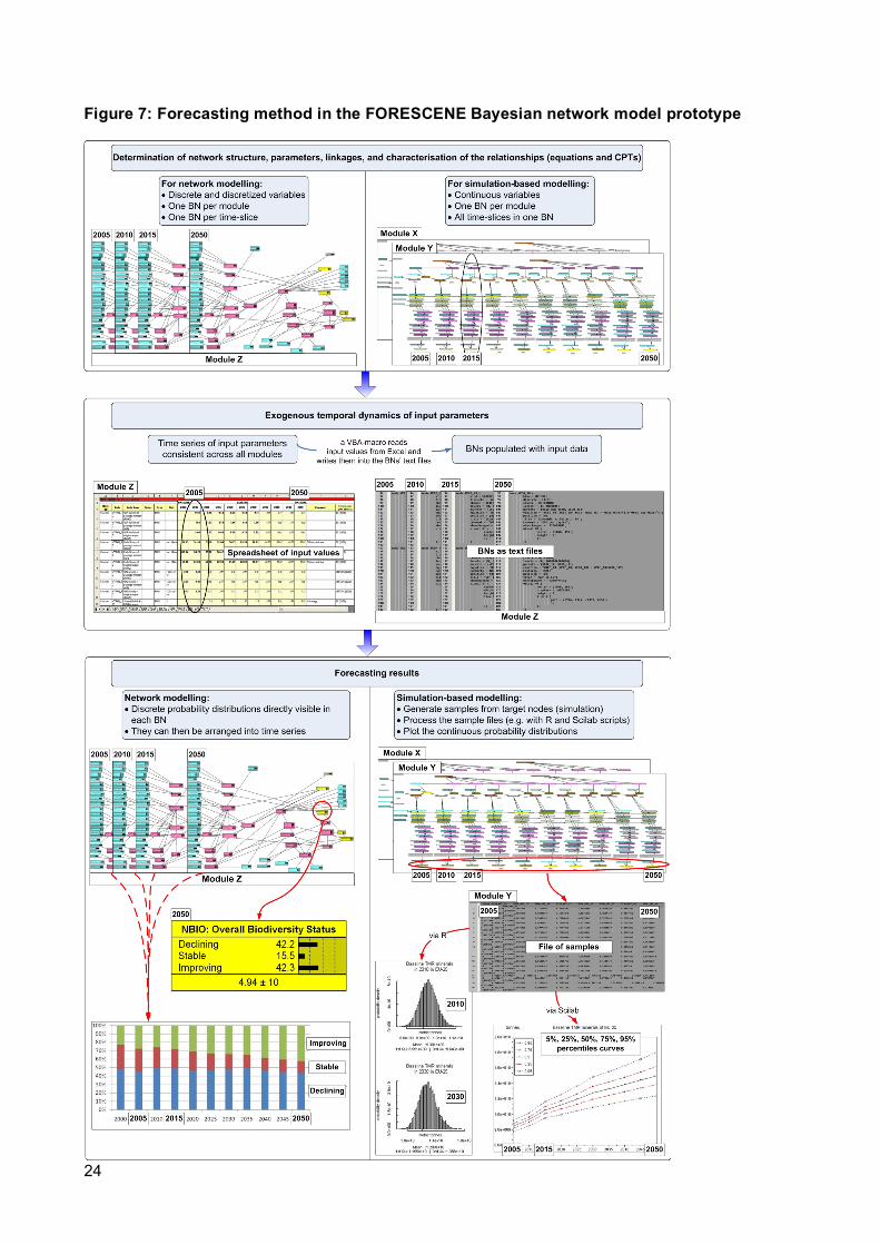
This section explains the forecasting technique used in FORESCENE. Figure 7 gives an overview
of the different steps involved. The upper, middle and lower parts of the figure summarize the
process into three phases:
! Construction of the network, parameterization and characterization of the linkages
! Construction of input data sets for each module
! Model runs, representation and analysis of the results.
The upper and lower parts of the figure are further divided into two boxes. On the left-hand side the
technical description concerns network modelling, while on the right-hand side simulation-based
modelling is described. The former option is reserved to BNs with discrete variables (e.g.
‘Agricultural management’ is ‘green’ or ‘brown’) or continuous variables that can be discretized
without increasing the variability of the results (e.g. ‘pollutant load’ with known thresholds). The
latter method regards BNs with continuous variables linked by functional equations, which would
be much less accurate if discretized.
Both approaches start with a graphical representation of the model structure (upper part of Figure
7). In FORESCENE, a commercial software called Netica1 was used. Parameters deemed
necessary to be considered can stem from participatory processes as in the Steps 1 and 2 of the
FORESCENE framework. The quantitative relationships characterizing the conditional distributions
between the model components need then to be established. The degree of belief and uncertainty
underlying the functional relationships between the variables is acknowledged through probabilities
in CPTs or equations with parameters expressed as probability distributions.
1 www.norsys.com

FORESCENE D.4.1-2 – Technical report
Baseline scenario assumptions and model projections for selected target indicators
23
Once the linkages are characterized, the marginal nodes (without parent nodes) are updated with
their probability distributions (discrete or continuous). Necessary information are read for each time
slice, for each marginal node of each module by a vba-macro from a common spreadsheet and
written into the text-file (i.e. non graphic) version of the BN.
When the model is “populated”, one can re-open its graphical version and run the forecast. With
discrete nodes and a compiled network (lower part, left-hand side of Figure 7) the modelled
probability distributions of target nodes over their discrete states (e.g. ‘Biodiversity status’ is
declining, stable or improving) can be read directly in Netica. Each time slice is modelled in a
separate BN. If an input node is modified, the influence of the change immediately appears.
For simulation-based modelling, sample cases should be generated (Netica has a Monte Carlo-like
function for it) in a sufficient number to cover the extent of the probability distributions of the target
nodes. Then, using the open source softwares for numeric calculation Scilab2 or for statistics R3,
these distributions can be visualised and their characteristics calculated. With the simulation-based
Bayesian modelling, results are more than single point values: the predictive precision, given
model uncertainties, of policy relevant variables is quantified.
2 www.scilab.org
3 www.r-project.org
24
Figure 7: Forecasting method in the FORESCENE Bayesian network model prototype

FORESCENE D.4.1-2 – Technical report
Baseline scenario assumptions and model projections for selected target indicators
25
3 Baseline assumptions for the input nodes
3.1 Resource use and waste generation submodel
3.1.1 Economy module
In its current stage of development, the model prototype does not feature an endogenous
representation of economic development. The economy module is not an econometric model.
Driving parameters such GDP per capita and population level are determined exogenously from
existing studies. The module then calculates GDP of EU-25 which level serves as a driver for
material and energy use, modelled in subsequent modules.
Projections of population growth are taken from Eurostat. From 2000 to 2015, population in EU-25
increases at a 1% rate per 5-year interval. The growth rate then slows down and becomes negative
from 2030 onwards. In 2050, the EU-25 hosts 2.3 million inhabitants less than in 2000.
Empirical data for GDP per capita (also referred to as economic activity) are taken from Eurostat
for the period 2000-2005 (7.5% increase over the period). For the period 2005-2020, an annual
average growth rate of 2% is taken for GDP per capita from the baseline of the GINFORS
economic model (MOSUS project). Other sources are slightly more optimistic, for example EEA
(2005) assumes an average annual growth rate of 2.5% for GDP per capita in the EU-25. To take
this observation into account and build the FORESCENE baseline scenario as a “corridor”
including both pessimistic and optimistic views, the growth of GDP per capita is modelled with a
normal distribution (mean = 2%, standard deviation = 0.3%). The distribution chosen is centred on
2% growth and 90% of its values occur in the interval 1.5%-2.5%. EC (2008), for example, uses a
+1.8% annual average growth rate in its baseline scenario. For the period 2020-2050, economic
activity is assumed to continue growing at a slower rate and is modelled with a normal distribution
centred on 1.5% (standard deviation = 0.3%).
As a result, real GDP increases on average by 2% per year until 2050. But, due to the uncertainty
about the growth rate of GDP per capita (represented by normal distribution), the confidence
interval around the mean value of GDP widens at each time step.
Domestic demand and exports are determined in comparison to GDP. In 2000, domestic demand
is as high as GDP4 while exports represent 36% of that value. The development trends given by
Eurostat until 2009 are prolonged until 2020 (-0.1% and +1.3% per year for the ratios domestic
demand and export to GDP, respectively). After that date, domestic demand and exports are
assumed to remain in the same proportions in comparison with GDP (98% and 51%, respectively).
3.1.2 Mineral materials module
Given the level of domestic demand5 and exports (see section on economy module), the domestic
material input of minerals (DMI minerals) of the European economy is driven by the respective
shares of services and goods in domestic demand and exports and their respective material
intensities. The corresponding input data are estimated from NAMEA6-based input-output analyses
4 At the EU-25 level, foreign trade is almost balanced (the difference between exports and imports represents
only 1% of GDP) which explains why domestic demand is as high as GDP.

26
conducted by the EEA ETC/RWM7 for 8 EU countries8 with monetary and physical IO tables from
1995 (2 countries) and 2000 (6 countries).
Averaging over the complete set of input-output results, the share of services9 in domestic demand
and export is estimated at 64% and 19%, respectively. These input values are assumed constant
over the whole timeframe in the baseline scenario.
Uncertainties arise from the sometimes questionable accuracy of the input-output analyses and
from scaling up the results for application at the EU-25 level. For example, MFA results for Europe
(Eurostat 2002, Moll et al. 2005, Schütz 2007) have been used to re-calibrate material intensities
which come out too high from the input-output analyses (because indirect foreign used extraction
associated with imports is included in the material inputs activated by final use of a product,
whereas DMI contains only imports and domestic used extraction). The proportionality relation
between material intensities of services vs. that of goods is preserved in the process. The point
values found for different material intensities in 2000 are presented in Table 2. Furthermore, it is
usually considered that DMI bears with itself an error of ±5% (we consider it as the 90% confidence
interval). To account for it, material intensities are modelled as normal distributions parameterised
with means as shown in Table 2 and standard deviations of 3% of the mean.
Table 2: Mean material intensity values in EU-25 in 2000
DMI activated
by final use
t / Mill. euros
Metal ores Industrial
minerals
Construction
minerals Total minerals
Goods 52 47 440 539
Services 5 7 69 81
The material intensity of goods is expected to decrease by 1.7% per year in the baseline scenario,
i.e. without the implementation of any particular policy instrument. It reflects the observed inherent
5 Includes the items “Final consumption expenditure by households”, “Final consumption expenditure by non-
profit organisations serving households (NPISH)”, “Final consumption expenditure by government”, “Gross
fixed capital formation” and “Changes in inventories and valuables”.
6 NAMEA: National Accounting Matrix including Environmental Accounts.
7 European Topic Centre on Resource and Waste Management (ETC/RWM, Topic Centre of the European
Environment Agency): Implementation Plan 2006 - task 7.1.2.1 "NAMEA-based Input-Output Analyses".
8 Germany, Denmark, Spain, Hungary, Italy, The Netherlands, Sweden and the United Kingdom.
9 The term ‘services’ includes the aggregated product groups “Wholesale and retail trade, repair of motor
vehicles, motorcycles and personal and household goods; hotels and restaurants; transport, storage and
communication”, “Financial intermediation; real estate, renting and business activities” and “Public
administration and defence, compulsory social security; education; health and social work; other community,
social and personal service activities; private households with employed persons; extra-territorial
organizations and bodies”. The term ‘goods’ corresponds to the aggregated product groups “Agriculture,
hunting, forestry and fishing”, “Total industry (excluding construction)” and “Construction”.

FORESCENE D.4.1-2 – Technical report
Baseline scenario assumptions and model projections for selected target indicators
27
increase of material productivity. Further improvement is not expected to occur in the baseline.
Material intensities of services are assumed constant.
The self-sufficiency of EU regarding minerals (i.e. the imported share of DMI minerals) is taken
from EU-15 MFA studies (Schütz 2007). According to the same source, the share of imports in DMI
metal ores and industrials minerals increased on average by 1.5% and 1.8 % per year during the
decade 1990-2000 (from 62% and 24% up to 72% and 29%, respectively). This trend is prolonged
until 2020 and the share of imports is assumed to remain constant afterwards. Imports of
construction minerals are neglected in view of the massive domestic extraction (mainly sand,
gravels, stones etc).
Moving from direct material input (DMI) to total material requirement (TMR), the indirect flows (IF)
associated with imports and the unused domestic extraction associated with mining in Europe (or
hidden flows, HF) need to be calculated. Hidden flows and indirect flows coefficients come from
EU-15 MFA studies (see Table 3). For the baseline, the trends observed in the decade before 2000
are prolonged until 2020 and flattened afterwards. Depending on the type of mineral materials,
domestic hidden flow and foreign indirect flow intensities are expected to further decrease, and
respectively increase, until 2020 at annual average rates presented in Table 3. TMR is usually said
to come with an error of ±15% (we consider it as the 90% confidence interval). To account for it
(including the error already coming with DMI), HF and IF coefficients are modelled as normal
distributions parameterised with means as shown in Table 3 and standard deviations of 9% of the
mean.
Table 3: Mean values for hidden and indirect flow coefficients for EU-25 in 2000 and baseline assumptions for the development until 2020 (mineral materials)
t / t Metal ores Industrial
minerals
Construction
minerals Total minerals
Hidden flows of
domestic extraction 1.07 0.43 0.22 0.56
Annual change until
2000-2020 -2.9% -3.1% -0.3% -0.9%
Indirect flows of
imports 13 4.01 : 8.09
Annual change until
2000-2020 +1.9% +3.8% : +1.1%
3.1.3 Fossil fuels module
The use of fossil fuels in the EU has in common with the use of mineral materials modelled in the
previous module the issues of extraction of non renewable resources, and the associated indirect
flows and unused extraction. The problem of greenhouse gases emissions is, however, specific to
this category of materials, mainly burnt for energy generation.

28
Table 4 presents the initial conditions (year 2000) and the assumptions for the dynamics of the
energy intensity and energy mix parameters in the baseline scenario. The data come from EC
(2008) until 2030. For the baseline, it is assumed that the parameters remain constant afterwards.
The basic reasoning behind is that any assumption according to which past rates of change, which
had been observed over about a decade, will continue for a period longer than 20 years in the
future would be highly uncertain. Increasing uncertainty could have been reflected by widening the
percentile corridor; this might have lead to unacceptable vagueness of results. One may also argue
that growth or decrease rates of input parameters will level off with time in a baseline scenario (i.e.
without specific strategies implemented to sustain and foster growth or decrease of key driving
factors). Following this rationale, rates of changes are either reduced past 2030 (e.g. in the
economy module) or parameters are simply kept constant. The resulting non-linearity of the
baseline forecasts provide also evidence of the impact of ongoing rates of change. The fossil fuel
mix is implemented partly exogenously to calculate the direct material input of fossil fuels (DMI
fossil fuels) of EU-25, starting from primary energy use. Conversion factors of primary energy into
mass of fuel are taken from EU tables reported to UNFCCC.
The degree of self-sufficiency of Europe regarding fossil fuels, hidden flow (HF) and indirect flow
(IF) coefficients for the domestic and foreign parts of DMI fossil fuels are adapted from the material
flow data base of the WI. The energy mix is taken into account exogenously in the overall
spreadsheet of input values (see section 2.7) and aggregated values are then read into the
Bayesian network model. This way, the complexity and number of ramifications of the network can
be kept at a manageable level. Table 5 shows HF and IF factors, and their development over time
assumed in the baseline. Trends observed over the period 1990-2000 for EU-15 (WI MFA data
base) show little to no change. These flat trends are prolonged until 2020 and parameters are kept
constant afterwards. Only hidden flow coefficients associated with domestic extraction of solid fuels
and natural gas show a slight increase. With the deposits reaching near depletion levels, unused
extraction increases for the same output of usable material. The availability and quality of data is
quite disparate, hence HF and IF coefficients are modelled as normal distributions parameterised
with means as shown in Table 5 and standard deviations of 5% of the mean.
Table 4: Baseline assumption for gross inland energy consumption (GIC) (EC 2008)
Initial conditions (year 2000) 2000-10 2010-20 2020-30 2030-50
toe GIC / Mill. Euro GDP Annual average % change
Energy intensity 170.4 -1.3 -1.7 -1.6 0
% of gross inland consumption Annual average % point change
Solid fuels 14.8 -0.1 +0.07 -0.03 0
Oil 40.4 -0.23 -0.08 -0.02 0
Natural gas 23.3 +0.2 +0.08 -0.01 0
Nuclear 15.3 -0.1 -0.25 -0.15 0
Renewable energy forms 6.0 +0.22 +0.19 +0.19 0

FORESCENE D.4.1-2 – Technical report
Baseline scenario assumptions and model projections for selected target indicators
29
Table 5: Mean values for hidden and indirect flow coefficients for EU-25 in 2000 and
baseline assumptions for the development until 2020 (fossil fuels and nuclear)
t / t Solid
fuels Oil Natural gas Nuclear Total fuels
Hidden flows of
domestic
extraction
7.15 0.01 0.1 : 4.4
Annual change
until 2000-2020 1.52% 0% 1.94% : 1.6%
Indirect flows of
imports 5.95 0.32 0.28 8500 1.8
Annual change
until 2000-2020 0.02% 0% 0% 0% 0%
3.1.4 Transport module
The transport module consists of a separate simplified transport model featuring road transport for
passengers and freight, and air transport for passengers. At the present stage of development of
the model prototype, the focus is to eventually determine the demand for biofuels in road transport
in order to link to the land use and greenhouse gas emissions modules.
The initial (year 2000) activity in freight (road) and passenger (air and road) transport are taken
from Eurostat (EU-25). The evolution of these parameters over time is modelled through elasticity
coefficients relating to the level of GDP growth (provided by the economy module). The baseline
scenario uses elasticities as shown in Table 6. Data up to 2030 come from the baseline scenario of
EC (2008) and are prolonged until 2050. Fuel efficiencies and improvement over time for each type
of transport are also taken from the baseline scenario of EC (2008).
The branch of the module dealing with road transport is then further expanded to model use for
biofuels. Seventy-five percent of the demand for biofuels is assumed to be covered by biodiesel
(own assumption, based on discussions with experts), the rest being bioethanol. The share of
biofuel actually blended with conventional fuel in 2000 and 2005 is taken from Eurostat. From then
until 2030, the baseline scenario values of EC (2008) are used (7.4% in 2020; 9.5% in 2030). After
2030, the highest objective of the EU Biofuel Directive (10%) is used until 2050.
Table 6: Baseline assumptions for the transport module
Unit Initial conditions (year
2005)
Evolution over time (2000-2050)
EU freight transport
(road)
Mt-km 1 793 390
GDP elasticity: 1.07 (2005-2010); 0.86
(2010-2015); 0.78 (2015-2020); 0.62
after 2030
EU passenger
transport (road)
MP-km 5 247 640 GDP elasticity: 0.58 (2005-2010); 0.54
(2010-2015); 0.53 (2015-2020); 0.51
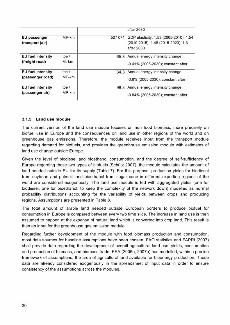
30
after 2030
EU passenger
transport (air)
MP-km 507 071 GDP elasticity: 1.53 (2005-2010); 1.54
(2010-2015); 1.48 (2015-2020); 1.3
after 2030
EU fuel intensity
(freight road)
toe /
Mt-km
65.3 Annual energy intensity change:
-0.41% (2005-2030); constant after
EU fuel intensity
(passenger road)
toe /
MP-km
34.3 Annual energy intensity change:
-0.8% (2005-2030); constant after
EU fuel intensity
(passenger air)
toe /
MP-km
98.3 Annual energy intensity change:
-0.84% (2005-2030); constant after
3.1.5 Land use module
The current version of the land use module focuses on non food biomass, more precisely on
biofuel use in Europe and the consequences on land use in other regions of the world and on
greenhouse gas emissions. Therefore, the module receives input from the transport module
regarding demand for biofuels, and provides the greenhouse emission module with estimates of
land use change outside Europe.
Given the level of biodiesel and bioethanol consumption, and the degree of self-sufficiency of
Europe regarding these two types of biofuels (Schütz 2007), the module calculates the amount of
land needed outside EU for its supply (Table 7). For this purpose, production yields for biodiesel
from soybean and palmoil, and bioethanol from sugar cane in different exporting regions of the
world are considered exogenously. The land use module is fed with aggregated yields (one for
biodiesel, one for bioethanol; to keep the complexity of the network down) modelled as normal
probability distributions accounting for the variability of yields between crops and producing
regions. Assumptions are presented in Table 8.
The total amount of arable land needed outside European borders to produce biofuel for
consumption in Europe is compared between every two time slice. The increase in land use is then
assumed to happen at the expense of natural land which is converted into crop land. This result is
then an input for the greenhouse gas emission module.
Regarding further development of the module with food biomass production and consumption,
most data sources for baseline assumptions have been chosen. FAO statistics and FAPRI (2007)
shall provide data regarding the development of overall agricultural land use, yields, consumption
and production of biomass, and biomass trade. EEA (2006a, 2007a) has modelled, within a precise
framework of assumptions, the area of agricultural land available for bioenergy production. These
data are already considered exogenously in the spreadsheet of input data in order to ensure
consistency of the assumptions across the modules.

FORESCENE D.4.1-2 – Technical report
Baseline scenario assumptions and model projections for selected target indicators
31
Table 7: Baseline assumptions regarding biofuel consumption for the land use module
Unit Initial conditions (year
2005)
Evolution over time (2000-2050)
EU share biodiesel %
(energy)
0.19 5.6% in 2020; 7.1% in 2030; 7.5%
afterwards
EU share
bioethanol
%
(energy)
0.06 1.9% in 2020; 2.4% in 2030; 2.5%
afterwards
EU self-sufficiency
in biodiesel
% 60 constant
EU self-sufficiency
in bioethanol
% 50 constant
Table 8: Baseline assumptions regarding biofuel yields for the land use module (outside EU)
Crops considered Yields (toe / ha)
Biodiesel produced
outside EU
Soybean and palm oil Normal distributions:
! = 1.9; ! = 0.4 in 2005
! = 2.8; ! = 0.6 in 2030
Bioethanol produced
outside EU
Sugar cane Normal distributions:
! = 2.5; ! = 0.3 in 2005
! = 3.7; ! = 0.4 in 2030
3.1.6 Greenhouse gases module
In the actual version of the model prototype, the output of the greenhouse gases module consists
of three main variables: greenhouse gas emissions from fossil fuels, greenhouse gas emission
savings from using biofuels instead of fossil fuels in road transport (excluding emissions from land
use changes due to biofuel production), and greenhouse gas emissions resulting from land
conversion for the production of biofuels. The GHG module is linked to the fossil fuel, transport and
land use modules that deliver the necessary inputs.
Regarding emissions from fossil fuels, the baseline assumptions presented in section 3.1.3 for the
energy mix, and especially the fossil fuel mix, translate as follows in terms of carbon intensity (EC
2008): in 2000 the economy of the EU emitted 2.23 tonnes of CO2 per tonne of oil equivalent (toe)
of gross inland energy consumption (all inclusive, i.e. with renewable sources); between 2000 and
2010 the carbon intensity is assumed to decrease on average by 0.3% per year; between 2020
and 2030 the carbon intensity is expected to decrease on average by 0.2% per year; and until
2050 the status quo is assumed as baseline.
With regard to emissions from the use of biofuels, Menichetti and Otto (2008) summarize activities
and findings of a comprehensive review of the most recent Life Cycle Assessment (LCA) studies
and energy and environmental balances of biofuels publicly available. For the model, the GHG

32
emissions saved life-cycle wide through the use of biofuels in the transport sector need to be
assessed for biodiesel and bioethanol produced in EU and outside (i.e. four estimates of GHG
savings needed). The geographical scope of the studies reviewed by Menichetti and Otto (2008)
usually does not match that of the EU-25. The overall GHG saving ranges given by the different
LCAs considered together are very wide for each of the four types of biofuels. To reflect these
results, normal distributions are built from the data in Menichetti and Otto (2008), assuming that the
ranges given in their review represent 99.8% confidence intervals (i.e. 3.09 standard deviations) for
the GHG emissions improvement compared to conventional fuel. The baseline assumptions finally
retained are presented in Table 9 and are assumed constant for the whole timeframe.
However, the emission savings calculated using LCAs data from the literature do not tell the whole
story because they overlook emissions induced by the conversion of natural land into arable land in
order to grow biofuel crops. This land use change is modelled in the previous module for biofuel
production outside Europe dedicated to the supply of Europe. The methodological framework and
baseline data uses Fargione et al.’s (2008) study. Table 10 shows the ‘carbon debt’ caused by the
conversion of 1 ha of natural land. Large variations of the carbon debt can be observed depending
on the region of production, and hence the type of land converted. These variations are captured in
the baseline assumptions shown in Table 10 in the form of normal probability distrbutions.
Table 9: GHG emissions improvements due to the use of biofuels compared to conventional
fuel (without land use change)
Crops considered
GHG emissions improvement
compared to conventional fuel
Biodiesel produced in
EU
Rapeseed Range: 20% - 80%
Normal distribution: ! = 50; ! = 9.7
Biodiesel produced
outside EU
Soybean and palm oil Range: -17% - 110%
Normal distribution: ! = 46.5; ! = 20.5
Bioethanol produced
in EU
Wheat Range: 2% - 90%
Normal distribution: ! = 46; ! = 14.2
Bioethanol produced
outside EU
Sugar cane Range: 70% - 100%
Normal distribution: ! = 85; ! = 4.9
Table 10: Carbon debt
Crops considered Carbon debt (t CO2 / ha)
Land converted for
biodiesel production
Soybean and palm oil Range: 33.2 - 1125.8 t CO2 / ha
Normal distribution: ! = 580; ! = 177
Land converted for
bioethanol production
Sugar cane Range: 57 - 165 t CO2 / ha
Normal distribution: ! = 111; ! = 17

FORESCENE D.4.1-2 – Technical report
Baseline scenario assumptions and model projections for selected target indicators
33
3.2 Water use submodel
The baseline assumed certain specific values for driving variables, updated each fifth year. These
key variables were given a certain value, assuming either a stable value for the period 2000-2050,
linear increase of exponential increase for the period. The baseline scenario was run with the
following set of input values below.
Cooling water efficiency (LA1) – The efficiency was assumed to remain the same throughout the
period. The EPRI report (2002) states that “it is unclear whether total U.S. freshwater consumption
by the power generation sector will increase or decrease over the next twenty years”. It is assumed
that the same will be valid for the European energy sector.
Industrial water efficiency (LB1) – The efficiency is assumed to increase linearly during the time
period (Cosgrove & Rijsberman, 2000). The efficiency is increasing from a level of 59% to 68%
during the time period.
Household water efficiency (LC1) – The household water efficiency is assumed to increase in a
linear fashion during the time period to 2050, from a level of 69% to 78%, as a result of the
introduction of water pricing and improved technology (Hoekstra & Chapagain, 2007).
Forested area (LF) – The forested area of Europe is expected to continue to increase, with a net
formation rate of new forested area of 0.5%/yr (EEA 2005; Eurostat 2007b).
Evapotranspiration (LG) – The rate of evapotranspiration is mainly determined by climatic factors,
and as the climate change is highly likely to continue, with higher temperatures over vast areas of
Europe (IPCC 2007), this will also lead to increased evapotranspiration. The evapotranspiration is
calculated to increase from 52% to 54% during the time period.
Irrigated area (LJ) – The climate change will also lead to an increase in the amount of irrigated
areas, especially in the southern parts of Europe. It is expected here that the amount will increase,
from a level of 25 million ha to 43 million ha in 2050 (EEA, 2007b).
Desalinized water (LN) – The climate change will also drive the amount of desalinisation of sea
water made. The current level of 1.2 billion m3 per year is expected to increase exponentially to a
level of 80 billion m3 per year (Aquastat 2007).
Recycled wastewater (LR) – Recycled wastewater is assumed to increase exponentially during the
period, from a very low level of 0.025 billion m3 per year to 6.4 billion m3 per year (EEA 2007b).
Precipitation (LT) – Most climate models project increasing precipitation rates for central and
northern Europe and decreasing precipitation rates for southern Europe and more intense rainfall
events (EEA 2007b). It is there assumed a modest increase of 5% during the 2000-2050 period.
Water quality (LWQ) – Water quality is assumed to remain the same during the period, affecting
around 5% of the total amount of available water, by making it unusable (EEA 2007b).

34
Table 11: Baseline assumptions for the water submodel
Node Label Unit 2005 2010 2015 2020 2025 2030 2035 2040 2045 2050
LA1 Cooling
water
efficiency
%
10
10
10
10
10
10
10
10
10
10
LB1 Industrial
water
efficiency
%
59 60 61 62 63 64 65 66 67 68
LC1 Household
water
efficiency
%
69 70 71 72 73 74 75 76 77 78
LF Forested
Area
106 ha
158 160 165 170 175 180 185 190 195 200
LG Evapotrans
piration
% 52 52 53 53 54 54 55 55 56 56
LJ Irrigated
area
106 ha
25 27 29 31 33 35 37 39 41 43
LN Desalinized
water
109 m
3
/year 0,31 0,40 0,60 1,20 2,40 4,80 10,0 20,0 40,0 80,0
LR Recycled
wastewater
109 m
3
/year 0,025 0,025 0,05 0,10 0,20 0,40 0,80 1,60 3,20 6,40
LT Precipitation 109 m
3
/year 1 355 1 360 1 365 1 370 1 375 1 380 1 385 1 390 1 395 1 400
LWQ Water
quality
% 5 5 5 5 5 5 5 5 5 5
3.3 Biodiversity, soils and landscape submodel
The following sections specify the baseline assumptions for the sub-model biodiversity, landscape
and soils. Recent and projected trends for the input parameters are described together with the
data sources from which the trend information was either derived or based. Table 11 at the end of
Section 3.2 provides an overview summary of the modelled trends for the sub-model input nodes.
3.3.1 Biodiversity and landscape module
The agri-environment support node represents the proportion of Common Agricultural Policy Pillar
II (Rural Development) spending on agri-environment programmes. The baseline data (2000) is
derived from mid-term Rural Development reports by Member States/regions, giving an overview
on agri-environmental measures applied in the 2000-2006 Rural Development programming period
(European Commission, 2003; European Commission Directorate General for Agriculture and
Rural Development, 2005). EU Member States report a wide range of proportionate spending on
agri-environment measures and a mean value was used to establish the baseline. In the
subsequent rural development period, 2007-2013, expenditure on agri-environment measures has
been reported at 22% of the EAFRD budget (European Commission, 2007). As a result the model
includes a growth in the expenditure on agri-environment programmes at the start of the period
2000-2050. Due to a lack of data on spending beyond 2013 it is assumed that the probability that
spending on AEP will be greater or less than 50% of the total spent on Pillar II of the CAP will

FORESCENE D.4.1-2 – Technical report
Baseline scenario assumptions and model projections for selected target indicators
35
follow a similar trend to that reported previously, i.e. it will show a small increase over each five-
year time step (Table 12).
Table 12: Probability of percentage spend on AEP
Year 2000 2005 2010 2015 2020 2025 2030 2035 2040 2045 2050
Probability % % % % % % % % % % %
AEP < 50% of Pillar II 85 85 78 78 69 69 58 58 47 47 36
AEP > 50% of Pillar II 15 15 22 22 31 31 42 42 53 53 64
Alliance Environnement, 2007 reports that non-adherence to cross compliance is approximately
12% (prior to 2005 there was no requirement for cross compliance so the model is set to 100%
non-compliance). Due to the short time cross compliance regulations have been in operation data
is fairly limited and predictions of future trends are, therefore, not available. Despite the lack of
predictive data to inform the model it has been assumed that the level of non-compliance will
decrease over the modelling period and a one-percent reduction in non-compliance has been
assumed for each model run (Table 13).
Table 13: Probability of non-compliance with cross compliance regulations
Year 2000 2005 2010 2015 2020 2025 2030 2035 2040 2045 2050
Probability % % % % % % % % % % %
>10% non-
compliance 100 90 89 88 87 86 85 84 83 82 81
<10% non-
compliance 0 10 11 12 13 14 15 16 17 18 19
The quality of forest management is difficult to assess; in the model forest management is defined
as either ‘green’ or ‘brown’. One indicator of forest management quality that can be used to
determine ‘green’ or ‘brown’ status is the area of forest that has been certified by the two main
certifying bodies operating in Europe (the Forest Stewardship Council and the Pan European
Forest Certification Council). Thus in the model ‘green management’ is taken to be the proportion
of forest area under certification. The ‘UNECE FAO Forest Products Annual Market Review (2006)’
reports that the area of certified forest increased by 12% between 2005 and 2006. However, the
figures for Europe show that over the same period the growth in certified forest area was much
smaller from 78.5 million hectares in 2005 to 78.9 million hectares in 2006, representing an annual
increase of about 0.5% (Table 14). An increase of 0.5% per annum is, therefore, assumed in this
model from 2005 onwards.

36
Table 14: Certified forest area by region, 2005-2006
Region Total forest
area
(million ha)
Total certified forest
area 2005 2006
(million ha)
Area certified
2005 2006
(% of total forest)
North America 470.6 140.2 157.7 29.8 33.5
EU/EFTA *155.5 78.5 78.9 50.5 50.7
EECCA 907.4 8.8 13.0 1.0 1.4
Oceania 197.6 3.4 6.4 1.7 3.3
Africa 649.9 6.2 2.1 1.0 0.3
Latin America 964.4 2.3 11.1 0.2 1.1
Asia 524.1 0.8 1.1 0.2 0.2
World total 3869.5 240.2 270.3 6.2 7.0
* Total forest area in this table refers to forest area only. Nodes LF, LFr have larger values as they include
areas classified as both forest and other wooded land (see Appendix 1).
(Source:UNECE/FAO Forest Products Annual Market Review, 2005-2006)
The conservation status of habitats data is derived from Article 17 reporting requirements under the
Habitats Directive (European Commission, 1992) for the period 2001-2006 for the EU2510. A major
component of the report is an assessment of the conservation of all habitats listed on Annexes I
and II of the Directive. The assessment is based around the definition of ‘favourable conservation
status’ set out in the directive, and combines assessments of range, area, structure and functions
and future prospects. Each of the parameters is reported as one of four classes, favourable,
unfavourable-inadequate, unfavourable and unknown. When the results from all four assessments
(range, area and so on) are unequal the results are weighted according to the following rules:
! If more than 25% is unfavourable bad then the result is unfavourable bad
! If more than 75% is favourable then the result is favourable
! If more than 25% is unknown then the result is unknown
! All other combinations the result is unfavourable-inadequate.
For the purpose of this model assessments returning the parameter value unknown have been
equally distributed between the other three categories. Combining the results of all four categories
makes an overall assessment; the habitat status nodes for 2000-2005 are populated with this data,
which was used to build the conditional probability tables. As noted above the assessment includes
a prediction of future prospects for conservation status for the subsequent reporting period. The
future prospects data has been used to establish the trends in future conservation status from 2010
(Figure 8). From 2015 onwards it is assumed that the trends in habitat status will continue as
10 http://biodiversity.eionet.europa.eu/article17/habitatsprogresswebsite

FORESCENE D.4.1-2 – Technical report
Baseline scenario assumptions and model projections for selected target indicators
37
suggested by the predictions made under Article 17 reporting. Taking the example of grassland this
would mean that the unfavourable – bad category will decrease, the unfavourable – inadequate
category will increase and finally that the favourable category would grow over the same time
frame. From 2005 to 2050, grassland habitat classified as bad would reduce from 46% to 19% of
total grassland area, that categorised as inadequate from 27 to 50% and grassland with favourable
conservation status would increase from 19% to 31%.

38
Figure 8: Expected changes in habitat status from 2000-2050 under baseline projections
(input nodes)
0%
20%
40%
60%
80%
100%
2000 2005 2010 2015 2020 2025 2030 2035 2040 2045 2050
Forest
Unfavourable – bad Unfavourable – inadequate Favourable
0%
20%
40%
60%
80%
100%
2000 2005 2010 2015 2020 2025 2030 2035 2040 2045 2050
Sclerophilus scrub
Unfavourable – bad Unfavourable – inadequate Favourable

FORESCENE D.4.1-2 – Technical report
Baseline scenario assumptions and model projections for selected target indicators
39
Figure 9: Expected changes in habitat status from 2000-2050 under baseline projections
(continued)
0%
20%
40%
60%
80%
100%
2000 2005 2010 2015 2020 2025 2030 2035 2040 2045 2050
Bogs and mires
Unfavourable – bad Unfavourable – inadequate Favourable
0%
20%
40%
60%
80%
100%
2000 2005 2010 2015 2020 2025 2030 2035 2040 2045 2050
Heath and Scrub
Unfavourable - bad Unfavourable - inadequate Favourable
0%
20%
40%
60%
80%
100%
2000 2005 2010 2015 2020 2025 2030 2035 2040 2045 2050
Aquatic
Unfavourable – bad Unfavourable – inadequate Favourable

40
Data on the conservation status of mammal and plant species is also derived from Article 17
reporting requirements under the Habitats Directive (European Commission, 1992) for the period
2001-2006 for the EU2511. The assessment is based around the definition of ‘favourable
conservation status’ set out in the directive, and combines assessments of range, population,
suitable habitat and future prospects. Each of the parameters is reported as one of four classes,
favourable, unfavourable-inadequate, unfavourable and unknown. For the purpose of this model
assessments returning the parameter value unknown have been equally distributed between the
other three categories (Table 15). As for habitat data when the results from all four assessments
(range, population and so on) are unequal the results are weighted according to the rules detailed
above. The future prospects data has been used to establish the trends in conservation status from
2010. From 2015 onwards it is assumed that the trends in habitat status will continue as suggested
by the predictions made under Article 17 reporting.
Table 15: Conservation status for mammal and plant species 2000-2005 and projections for 2010
Species Group Conservation Status 2000 2005 2010
Unfavourable – bad
35.0% 35.0% 29%
Unfavourable – inadequate
36.0% 36.0% 33% Mammal species status
Favourable
29.0% 29.0% 38%
Unfavourable – bad
28.0% 28.0% 20%
Unfavourable – inadequate
43.0% 43.0% 42% Plant species status
Favourable
29.0% 29.0% 38%
The following figures illustrate the probability that plant and mammal species will be assessed as
unfavourable – bad, unfavourable – inadequate and favourable for the period 2000-2050. These
figures suggest that that the conservation status of these two species groups will improve and that
by 2020 for plant species and 2025 for mammal species conservation status is more likely to be
favourable than either of the two unfavourable categories.
11 http://biodiversity.eionet.europa.eu/article17/habitatsprogresswebsite

FORESCENE D.4.1-2 – Technical report
Baseline scenario assumptions and model projections for selected target indicators
41
Figure 10: Expected changes in species status from 2000-2050 under baseline projections
(input node)
0%
20%
40%
60%
80%
100%
2000 2005 2010 2015 2020 2025 2030 2035 2040 2045 2050
Mammals
Unfavourable – bad Unfavourable – inadequate Favourable
0%
20%
40%
60%
80%
100%
2000 2005 2010 2015 2020 2025 2030 2035 2040 2045 2050
Plants
Unfavourable – bad Unfavourable – inadequate Favourable
The BirdLife (2004b) found that, 216 (48%) species out of 448 species had unfavourable
conservation status at the EU25 level. This showed that there is a higher proportion of species with
unfavourable status in the EU25 than at the Pan-European level (43% unfavourable). To assess
the conservation status of all wild bird species occurring naturally and regularly in the European
Union Birdlife collected the following data from each country:
! Breeding population size (in or around the year 2000).
! Breeding population trend (over the period 1990–2000).
Wherever possible, national coordinators supplied population trend data as actual percentage
change figures over the period 1990–2000. Where this was not possible data was supplied on
trend direction and magnitude using a fixed set of categories and codes. Trend categories ranged
from -5 to 5, with the sign indicating the direction of the change and with stable populations being
represented by a value of zero. The conservation status of birds in the EU25 was assessed using
the three-step process illustrated in Figure 11.

42
Figure 11: Methodology for determination of EU25 conservation status for bird species
Looking at the situation in 1990, the percentage of species with unfavourable conservation status
at (today) EU25 level was slightly higher (51%) than in 2000. This suggests the overall situation of
birds has slightly improved in the EU and in the new joining countries. In line with this trend a 3%
decrease in the probability of unfavourable conservation status was taken forward for each five-
year time step (Table 16).
Table 16: Projected probability of favourable and unfavourable conservation status for EU25
bird species (input node)
Year 2000 2005 2010 2015 2020 2025 2030 2035 2040 2045 2050
Probability % % % % % % % % % % %
Unfavourable 48.0 46.6 45.0 43.5 42.1 40.6 39.2 37.8 36.4 35.0 33.6
Favourable 52.0 53.6 55.0 56.5 57.9 59.4 60.8 62.2 63.6 65.0 66.4

FORESCENE D.4.1-2 – Technical report
Baseline scenario assumptions and model projections for selected target indicators
43
Figure 12: Current trends in EU mammal and bird populations
Birds population trends
Decreasing
23%
Stable
51%
Increasing
9%
Unknown
17%
Mammal population trends
Decreasing
27%
Stable
32%
Increasing
8%
Unknow n
33%
The current status of mammal species, according to the 2007 publication ‘The Status and
Distribution of European Mammals’ (Temple and Terry, 2007), is that 27% of mammal species are
declining, 32% are stable, 8% are increasing and the final 33% have an unknown population trend
(Figure 12). These figures are used as the starting point for the model. ‘Global Biodiversity Outlook
2’ (Secretariat of the Convention on Biological Diversity, 2006), reports that vertebrate species
have declined by approximately 40% over the period 1970-2000. In line with this data an annual
increase in the probability of species declining of 1.3% per annum has been used to suggest
species trends for 2005-2050.

44
Figure 13: Projected probability of declining, stable, increasing or unknown trend in
mammal and bird populations (input nodes)
Mammals
0%
20%
40%
60%
80%
100%
2000 2005 2010 2015 2020 2025 2030 2035 2040 2045 2050
Declining Stable Increasing Unknown
Birds
0%
20%
40%
60%
80%
100%
2000 2005 2010 2015 2020 2025 2030 2035 2040 2045 2050
Declining Stable Increasing Unknown
Birdlife 2004 report that in 2000 51% of bird species populations were stable, 23% were
decreasing and 9% were increasing (Figure 13). In comparison with the figures for the 1990
assessment species were more likely to have moved from the decreasing to stable category than
vice versa. For that reason the projected probability of stable population increases from 51% to
65% over the period 2000-2050 (Figure 13).
Invasive alien species are non-native species that have been introduced by human action (either
intentionally or unintentionally) outside their natural habitats where they have established and bred
causing damage to biological diversity. Invasive alien species present a significant threat to
European biodiversity, acting as vectors for disease, altering the structure and functioning of the
ecosystem and competing for food and resources with native species. Globally invasive alien
species are considered as a second major threat to biodiversity and at the EU level both the EU 6th
Environmental Action Programme and the 2006 communication from the Commission of Halting
the Loss of Biodiversity by 2010 and beyond have identified invasive alien species as a priority
area for action.
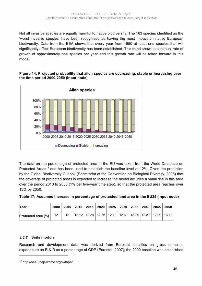
FORESCENE D.4.1-2 – Technical report
Baseline scenario assumptions and model projections for selected target indicators
45
Not all invasive species are equally harmful to native biodiversity. The 163 species identified as the
‘worst invasive species’ have been recognised as having the most impact on native European
biodiversity. Data from the EEA shows that every year from 1950 at least one species that will
significantly affect European biodiversity has been established. This trend shows a continual rate of
growth of approximately one species per year and this growth rate will be taken forward in this
model.
Figure 14: Projected probability that alien species are decreasing, stable or increasing over
the time period 2000-2050 (input node)
0%
20%
40%
60%
80%
100%
2000 2005 2010 2015 2020 2025 2030 2035 2040 2045 2050
Alien species
Decreasing Stable Increasing
The data on the percentage of protected area in the EU was taken from the World Database on
Protected Areas12 and has been used to establish the baseline level at 12%. Given the prediction
by the Global Biodiversity Outlook (Secretariat of the Convention on Biological Diversity, 2006) that
the coverage of protected areas is expected to increase the model includes a small rise in this area
over the period 2010 to 2050 (1% per five-year time step), so that the protected area reaches over
13% by 2050.
Table 17: Assumed increase in percentage of protected land area in the EU25 (input node)
Year 2000 2005 2010 2015 2020 2025 2030 2035 2040 2045 2050
Protected area (%) 12 12 12.12 12.24 12.36 12.49 12.61 12.74 12.87 12.99 13.12
3.3.2 Soils module
Research and development data was derived from Eurostat statistics on gross domestic
expenditure on R & D as a percentage of GDP (Eurostat, 2007); the 2000 baseline was established
12 http://sea.unep-wcmc.org/wdbpa/

46
as 1.9%. Despite the target set by the Lisbon summit for research expenditure to reach 3% of GDP
by 2010 there has been little change in the proportionate spending on R & D over the last decade
(Figure 10). In line with these findings the expenditure on GDP was assumed at a constant 1.9%.
Table 18: Projected share of gross domestic expenditure in R & D (% of GDP) (input node)
1995 1996 1997 1998 1999 2000 2001 2002 2003 2004
% of
GDP
1
.
9
1.8 1.8 1.8 1.9 1.9 1.9 1.9 1.9 1.9
Source: Eurostat Yearbook 2006-2007
Amongst the aims of the proposed Soil Framework Directive are the establishment of a common
framework to “protect soil on the basis of the principles of preservation of soil functions, prevention
of soil degradation, mitigation of its effects, restoration of degraded soils and integration in other
sectoral policies” (European Commission 2006, p.5). However, the Soil Framework Directive has
not yet been implemented. Despite this it was felt that the future introduction of such legislation
could have important implications for a number of soil-based parameters, which made this an
interesting node to include within the sub model. The baseline state for the Soil Framework
Directive has been set to ‘none’. Due to uncertainty about when the Directive will be implemented,
and in what format, the node is set to this state throughout the baseline scenario.
Estimates of greenhouse gas emissions at the global level serve as proxy for representing how
pressing the issue of climate is and will become. Greenhouse gas emission data is obtained from
IPCC data, which reports emissions of 44.7 Gt CO2-equivalent in the year 2000 (IPCC, 2007). Due
to the uncertainty associated with this estimate this is modelled as a normal distribution with a
standard deviation of about 5 Gt CO2- equivalent. The SRES13 Scenarios project an increase of
baseline global gas emissions of between 25 to 90% between 2000 and 2030. Beyond 2030, the
situation is less clear-cut with SRES scenarios predicting both increases and decreases in
greenhouse gas emission. However, data from the CAIT databases14 suggests that on average
emissions of CO2 (Mt CO2 from energy) will increase by an average of 1.5% between 2002 and
2050. Although not accounting for all sectors or all types of emissions this value is used as an
indication of future global greenhouse gas emissions and a 1.5% per annum increase is taken
forward in this model.
13 SRES scenarios are those described in the IPCC Special Report on Emissions Scenarios (2000). The
scenarios are grouped into four families, A1, A2, B1 and B2, which explore a wide range of driving forces
(economic, demographic and technological) and their resulting greenhouse gas emissions.
14 http://cait.wri.org/

FORESCENE D.4.1-2 – Technical report
Baseline scenario assumptions and model projections for selected target indicators
47
Figure 15: Projected greenhouse gas emissions for the period 2000-2050 (input node)
0.0
20.0
40.0
60.0
80.0
100.0
120.0
2000 2005 2010 2015 2020 2025 2030 2035 2040 2045 2050
GT
CO
2 e
quiv
ale
nt
Greenhouse gas emissions
Nutrient transfer efficiency data is taken from a number of sources (Domburg et al., 2000, Raun
and Johnson, 1999; IGER) and so the baseline value has been established using a normal
distribution with mean values of 28% (standard deviation 14%) for grassland and 52% (standard
deviation 26%) for arable crops. Improvements in nutrient use efficiency might be expected in the
future, however, the level of increase in efficiency that might be expected is difficult to quantify. For
that reason the level of nutrient transfer efficiency is increased by one percent for each five year
time period.
Figure 16: Assumed nutrient transfer efficiency for grassland and arable from 2000-2050
(input node)
Nutrient transfer efficiency
0.0
20.0
40.0
60.0
80.0
100.0
2000 2005 2010 2015 2020 2025 2030 2035 2040 2045 2050
Grassland Arable
Fertiliser use intensity for the EU is taken from the CAIT database, 2002 data for EU 27 (excluding
Slovakia, Luxembourg and Latvia). Using this resource a mean and standard deviation were
calculated so that fertiliser use for the baseline year could be modelled as a normal distribution,
reflecting the variability of this statistic. The European Fertiliser Association (EFMA) (2007) predicts
an increase in the use of nitrogen in the EU27 of 3.6% between 2007 and 2017. In contrast, over

48
the same period EFMA suggest that the use of phosphorus will decline by 4.4% and potassium by
2.6%. The FAO report, World Agriculture: 2015/2030 suggests that overall fertiliser use will
continue to grow in the developed world until 2030 by about 1% per annum. This latter figure
represents all nutrient sources so was used to represent the growth in fertiliser use intensity until
2030. Beyond 2030, the direction of future fertiliser use intensity is uncertain so between 2030 and
2050 the value in the baseline scenario will be held constant.
Figure 17: Projected change in fertiliser use intensity for the baseline scenario 2000-2050 (input node)
0
100
200
300
400
500
2000 2005 2010 2015 2020 2025 2030 2035 2040 2045 2050
kg/ha
Fertiliser use intensity

FORESCENE D.4.1-2 – Technical report
Baseline scenario assumptions and model projections for selected target indicators
49
4 Baseline forecasting results for selected intermediary and target
nodes
4.1 Resource use and waste generation submodel
This section presents baseline forecasts for key output nodes of the resource use and waste
generation submodel. As described in chapter 3, the use of probability distributions instead of point
values makes it possible to account for a degree of parameter uncertainty. As a consequence,
forecasts of target indicators are shown as “corridors” that represent the 90% confidence intervals
of the corresponding modelling results, given the input parameter uncertainties.
4.1.1 Economy module
In the economy module, future growth of GDP per capita is modelled using a normal distribution
centred in 2% until 2030 and in 1.5% afterwards (0.3% standard deviation in each case). Figure 18
(upper part) shows the baseline assumptions for population and GDP per capita in the EU-25. The
range defined by the normal distribution for GDP per capita was chosen to reflect differences in
assumptions observed in existing European scenario studies. The lower part of Figure 18 shows
the forecast for European GDP until 2050. The width of the confidence interval increases the
further we look into the future. Given the assumptions for the input parameters, GDP roughly
doubles between 2005 and 2050, though it is expected to increase at a slightly slower rate after
2030. Starting from the point value reported in European statistical data (about 10*106 million
euros), GDP’s mean value reaches about 21*106 million euros in 2050 (90% CI: 18.5 - 25.2 *106
million euros).
4.1.2 Mineral materials module
As a consequence of a growing economy, the 90% confidence interval for TMR minerals increases
from 7.8 – 9.2Gt in 2005 to 12.4 – 18Gt in 2050 (Figure 19). Though the direct material input levels
off over time, due to increasing material productivity and the assumption of a slower GDP growth
after 2030, TMR keeps increasing. This can be explained by the fact that the indirect flows,
especially unused extraction such as mining waste associated with direct material input, keep
increasing as a result of resource depletion. Furthermore, increasingly this waste production occurs
in other parts of the world that export to Europe. This worsening of the problem shifting is illustrated
by the ratio foreign TMR over domestic TMR in Figure 20, which keeps increasing. The forecasted
trend shows that in 2050 between 2.3 and 3.1 (90% CI) times more materials will be extracted, and
for a large part turned into waste, outside the EU than within in order to satisfy European demand
for mineral materials.
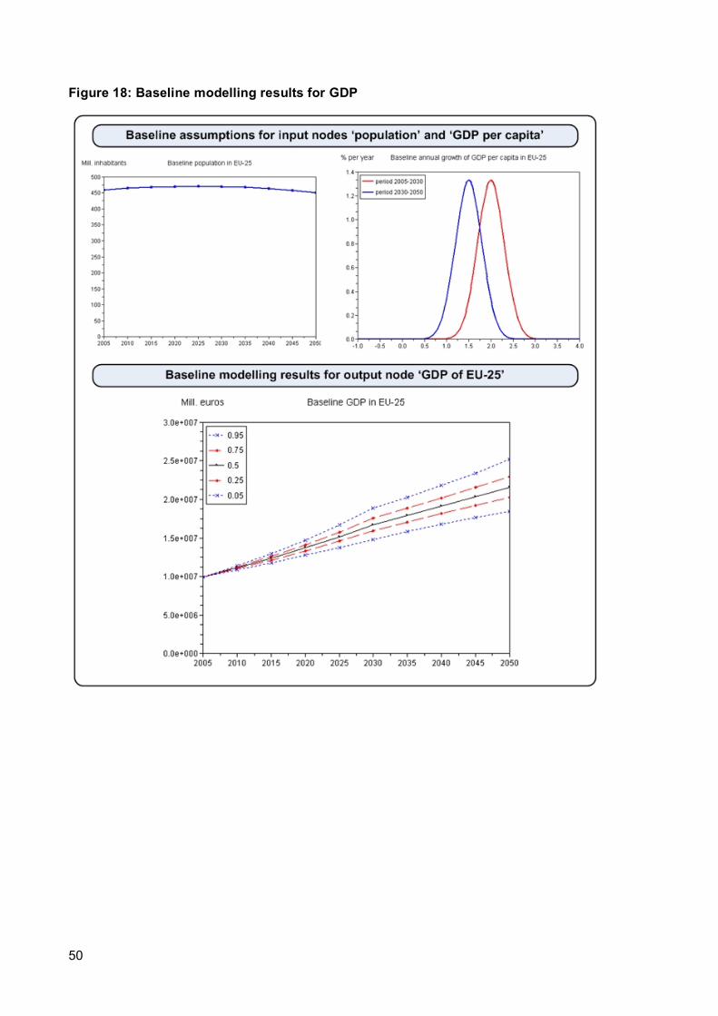
50
Figure 18: Baseline modelling results for GDP

FORESCENE D.4.1-2 – Technical report
Baseline scenario assumptions and model projections for selected target indicators
51
Figure 19: Baseline modelling results for TMR minerals
Figure 20: Baseline modelling results for the ratio foreign vs. domestic TMR minerals

52
4.1.3 Fossil fuels module
For the period 2005-2030, the assumptions for the baseline improvement in energy efficiency and
the development of renewable energy sources in EU-25 were derived from EC 2008, as described
in section 3.1.3. The development of these parameters compensate the joint effects of a growing
economy and growing indirect flows per unit of extracted fossil fuel. Therefore the mean value of
TMR fossil fuels remains rather constant around 6.5 billion tonnes (Figure 21). The 90% confidence
interval, however, gets wider from 6.3-6.9 to 5.7-7.5 billion tonnes reflecting the uncertainties built
in model parameters such as hidden and indirect flow coefficients in the present module, and
economic growth in the “parent” economy module. Baseline assumption that Europe will
increasingly rely on imported fossil fuels for its energy supply also explains that the ratio foreign vs.
domestic TMR increases until 2030 (Figure 22).
Regarding the 2030-2050 period, input parameters such as energy efficiency and development of
renewable energy sources are conservatively kept constant at the baseline level they are expected
to reach in 2030. At the same time, economy is assumed to keep growing (though at a slower rate)
which explains that mean TMR fossil fuels increases from 6.5 to 8.4 billion tonnes between 2030
and 2050 (Figure 21). It is also assumed that, after 2030, the import structure of Europe regarding
fossil fuels has stabilised and the share of imports remain constant at 78%. Therefore, the ratio
foreign vs. domestic TMR remains constant (Figure 22). It means that, in relative terms, the
situation will worsen at the same pace outside and inside EU. However, the absolute amount of
fossil fuels extracted and waste generated outside the EU keeps increasing and remains higher
than in the EU.

FORESCENE D.4.1-2 – Technical report
Baseline scenario assumptions and model projections for selected target indicators
53
Figure 21: Baseline modelling results for TMR fossil fuels
Figure 22: Baseline modelling results for the ratio foreign vs. domestic TMR fossil fuels

54
4.1.4 Transport module
Transport activities in the EU-25 are expected to be tight to economic growth, with elasticities
around 0.5 for passenger road transport, decreasing from 1 to 0.6 for freight road transport, and
remaining higher than 1 at 1.3-1.5 for passenger air transport. Expected activities in million tonne
kilometres and million passenger kilometres are shown in Figure 24. Following growth in road
transport and mandatory biofuel blending with conventional fuel (up to 9.5% in 2030 and constant
afterwards), biofuel use is expected to increase ten fold, from 3.3 to 34 million toe, between 2005
and 2030 (Figure 23).
Figure 23: Baseline modelling results for biofuel consumption

FORESCENE D.4.1-2 – Technical report
Baseline scenario assumptions and model projections for selected target indicators
55
Figure 24: Baseline modelling results for transport
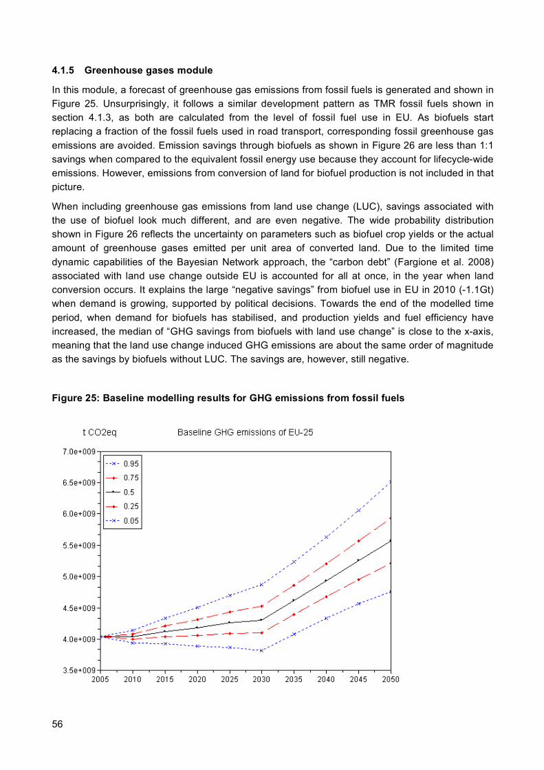
56
4.1.5 Greenhouse gases module
In this module, a forecast of greenhouse gas emissions from fossil fuels is generated and shown in
Figure 25. Unsurprisingly, it follows a similar development pattern as TMR fossil fuels shown in
section 4.1.3, as both are calculated from the level of fossil fuel use in EU. As biofuels start
replacing a fraction of the fossil fuels used in road transport, corresponding fossil greenhouse gas
emissions are avoided. Emission savings through biofuels as shown in Figure 26 are less than 1:1
savings when compared to the equivalent fossil energy use because they account for lifecycle-wide
emissions. However, emissions from conversion of land for biofuel production is not included in that
picture.
When including greenhouse gas emissions from land use change (LUC), savings associated with
the use of biofuel look much different, and are even negative. The wide probability distribution
shown in Figure 26 reflects the uncertainty on parameters such as biofuel crop yields or the actual
amount of greenhouse gases emitted per unit area of converted land. Due to the limited time
dynamic capabilities of the Bayesian Network approach, the “carbon debt” (Fargione et al. 2008)
associated with land use change outside EU is accounted for all at once, in the year when land
conversion occurs. It explains the large “negative savings” from biofuel use in EU in 2010 (-1.1Gt)
when demand is growing, supported by political decisions. Towards the end of the modelled time
period, when demand for biofuels has stabilised, and production yields and fuel efficiency have
increased, the median of “GHG savings from biofuels with land use change” is close to the x-axis,
meaning that the land use change induced GHG emissions are about the same order of magnitude
as the savings by biofuels without LUC. The savings are, however, still negative.
Figure 25: Baseline modelling results for GHG emissions from fossil fuels

FORESCENE D.4.1-2 – Technical report
Baseline scenario assumptions and model projections for selected target indicators
57
Figure 26: Baseline modelling results for GHG emissions savings from biofuel without land
use change
Figure 27: Baseline modelling results for GHG emissions savings from biofuel including land use change

58
4.2 Water use submodel
The water usage efficiencies within the industrial, power generation and household sectors are
assumed to increase linearly but modestly in a business-as-usual scenario, while industrial
recycling and desalinization are assumed to increase exponentially, starting from a low level. The
overall usage of water is expected to increase during the period, driven by increasing material and
energy use, which is outside the water sub-model boundaries. It is also assumed that the number
of households will continue to increase, even if the EU-25 population level remains stable, which
will lead to increase in overall household water consumption. The water balance (difference
between withdrawals and supply) is not expected to change significantly, as increasing
precipitations (as a consequence of climate change, especially in the north of Europe), recycling
and desalinization (especially in the south of Europe) tend to offset increased consumption.
Regional variations, however, can be expected to be more contrasted. But they are, to date, not
captured by the model prototype.
Figure 28: Baseline modelling results for total water withdrawals

FORESCENE D.4.1-2 – Technical report
Baseline scenario assumptions and model projections for selected target indicators
59
Figure 29: Baseline modelling results for water balance
4.3 Biodiversity, soils and landscape submodel
The biodiversity, soils and landscape sub-model consists of discrete and discretized nodes. In
order to reduce the problem of discretizing continuous variables (much information is often lost in
the process and the result can be misleading), for those nodes where the input parameter is
specified as a normal distribution with associated mean and standard deviation (Table 20) initial
model runs were undertaken using the mean value as a numeric input to the model. In addition,
due to lack of data from the water model at the time of the model runs, the value for water
abstraction was held constant (i.e. node LM1 change in water abstraction was set to 100%
probability that abstraction was stable). These considerations need to be borne in mind when
considering the initial model output presented below.
Figure 30 shows the modelled output for the nodes terrestrial, aquatic and overall biodiversity. The
model predicts that aquatic biodiversity status will improve over the period 2000-2050, i.e. there will
be a greater probability of favourable conservation status in 2050 than in 2000. However, it should
be remembered that the water abstraction node was held constant in this model run and allowing
this node to vary would produce more realistic results.
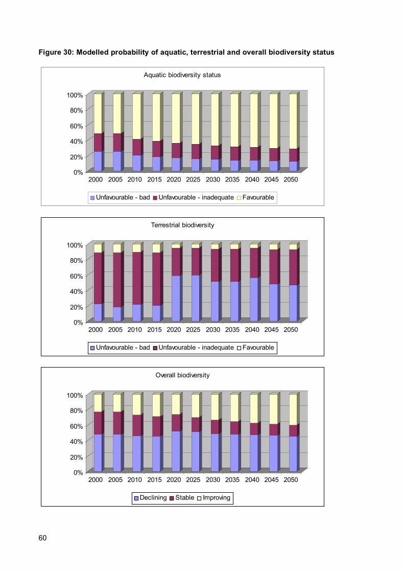
60
Figure 30: Modelled probability of aquatic, terrestrial and overall biodiversity status
0%
20%
40%
60%
80%
100%
2000 2005 2010 2015 2020 2025 2030 2035 2040 2045 2050
Aquatic biodiversity status
Unfavourable - bad Unfavourable - inadequate Favourable
0%
20%
40%
60%
80%
100%
2000 2005 2010 2015 2020 2025 2030 2035 2040 2045 2050
Terrestrial biodiversity
Unfavourable - bad Unfavourable - inadequate Favourable
0%
20%
40%
60%
80%
100%
2000 2005 2010 2015 2020 2025 2030 2035 2040 2045 2050
Overall biodiversity
Declining Stable Improving

FORESCENE D.4.1-2 – Technical report
Baseline scenario assumptions and model projections for selected target indicators
61
In contrast, the model predicts that terrestrial habitat condition will decline over the same period
with the probability of unfavourable habitat status increasing from 25% in 2000 to 48% by 2050.
At the start of the modelling period the model predicts a 48% probability that overall biodiversity will
be declining and an almost equal chance that it will be either stable or increasing. By the end of the
modelling period the model prediction there is a similar probability of declining biodiversity (45%) to
that predicted in 2000, a 14% chance that biodiversity will be stable and a 41% chance that it will
be increasing.
Figure 31 shows the predicted model probability for fragmentation, wider ecological potential and
protected habitat condition, three of the four parent nodes for terrestrial biodiversity. The fourth
parent node for terrestrial biodiversity is area of protected land, which is derived from exogenous
data. In line with the node for terrestrial biodiversity the model predicts that fragmentation will
increase and that the wider ecological potential will be reduced and that overall habitat condition is
most likely to be unfavourable. Looking at the charts in Figure 31 the effect of abrupt changes in
state can be seen. For example, the parents of the fragmentation node (effective mesh size) are
the discrete nodes artificial, forest and agricultural land use change. For the first four model runs
(2000-2015) these nodes are set so that land use is stable (probability 100%) and therefore, the
model predicts that the status of fragmentation will also remain stable. However, by 2020 assumed
changes in land use (set as input) mean that the model now works with a 100% probability that
agricultural area is decreasing, a 100% probability that artificial area is increasing and 100%
probability that forest area remains stable. This change in parent node states can be seen in the
fragmentation chart where the probability of high fragmentation (low MEFF) is now abruptly
increased.
Figure 32 shows the node for soil organic carbon, soil erosion and soil quality. The predicted
probability for these nodes shows little change under modelled conditions as the Soil Framework
Directive, which is a parent node of a number of soil related parameters has been kept constant at
‘none’ (100% probability) for the entire modelling period.
The model predicts that there will be an increase in favourable conservation status over the fifty-
year period 2000-2050. However, the model also suggests that there will be an increase in the
number of species that are experiencing a downward trend in species number.

62
Figure 31: Predicted model probability for soil erosion and soil carbon and the output node
soil quality
0%
20%
40%
60%
80%
100%
2000 2005 2010 2015 2020 2025 2030 2035 2040 2045 2050
Fragmentation
MEFF low MEFF medium MEFF high
0%
20%
40%
60%
80%
100%
2000 2005 2010 2015 2020 2025 2030 2035 2040 2045 2050
Ecological potential - wider landscape
Green index low Green index medium Green index high
0%
20%
40%
60%
80%
100%
2000 2005 2010 2015 2020 2025 2030 2035 2040 2045 2050
Protected habitat condition
Unfavourable - bad Unfavourable - inadequate Favourable

FORESCENE D.4.1-2 – Technical report
Baseline scenario assumptions and model projections for selected target indicators
63
Figure 32: Predicted model probability for soil erosion and soil carbon and the output node
soil quality
0%
20%
40%
60%
80%
100%
2000 2005 2010 2015 2020 2025 2030 2035 2040 2045 2050
Soil erosion
Soil Erosion 0-0.5 t/ha/yr Soil Erosion 0.5-1 t/ha/yr Soil Erosion 1-2 t/ha/yr
Soil Erosion 2-5 t/ha/yr Soil Erosion 5-10 t/ha/yr
0%
20%
40%
60%
80%
100%
2000 2005 2010 2015 2020 2025 2030 2035 2040 2045 2050
Soil carbon
0 to 1% SOC 1 to 2% SOC 2 to 6% SOC
0%
20%
40%
60%
80%
100%
2000 2005 2010 2015 2020 2025 2030 2035 2040 2045 2050
Soil quality
Low Medium High

64
Figure 33: Predicted model probability of species conservation status and trend in species
number
0%
20%
40%
60%
80%
100%
2000 2005 2010 2015 2020 2025 2030 2035 2040 2045 2050
Conservation status - species
Unfavourable Favourable
0%
20%
40%
60%
80%
100%
2000 2005 2010 2015 2020 2025 2030 2035 2040 2045 2050
Trend in species number
Decreasing Stable Increasing

FORESCENE D.4.1-2 – Technical report
Baseline scenario assumptions and model projections for selected target indicators
65
5 Conclusions
The forecasting method using network and simulation-based Bayesian modelling as presented in
this report provided a set of modelling results constituting the baseline scenario of FORESCENE.
The baseline will serve as reference against which alternative scenarios will be elaborated in
workpackage 5. A basic finding from the business-as-usual scenario is that current trends in
material and energy productivity improvements are insufficient to offset the growing demand for
resources that result from continued economic growth. It also shows that a large and increasing
part of the environmental burden associated with material and energy use in Europe actually hits
the environment outside our boundaries.
The modelling approach chosen allows to represent results for quantitative indicators as “corridors”
that reflect the 90% confidence interval. This represents the uncertainties attached to input and
control parameters. As a consequence, the width of the results’ confidence intervals (hence of the
corridor of probability) tend to increase the further we look into the future.
Besides the continuous full probability distributions of quantitative parameters, some more
qualitative indicators can also be represented. In such a case, modelling results take the form of
discrete probability distributions. Nodes are linked probabilistically through the result of expert
judgement and literature data elicitation. Thus the modelling framework allows the inclusion of both
physically measurable and calculated data and more qualitative assessments.
The baseline forecasts provide some first plausible as well as interesting outcomes. However,
more testing is recommended to check the robustness of the various facets of the model prototype.
Endogenous and exogenous linkages between the modules need to be further tested and
improved. The behaviour of the ‘biodiversity and soils’ sub-network, whose long ramifications of
discrete and discretized nodes tend to buffer the effect of influencing parameters situated
upstream, need to be studied closer.
Finally, there are three major options for further development.
Firstly, biodiversity outside the EU has not yet been included in the model explicitly. Nevertheless,
the model shows that the increased land use change for biofuel production leads to enhanced
GHG emissions, and therefore one may conclude that biodiversity in other regions is also
negatively affected. With the modelling of appropriate expert knowledge, this relation, as well as
others, could be modelled using a module made of discrete nodes, similarly to the modelling of
biodiversity within Europe.
Secondly, the modelling of agricultural land use could be extended to food biomass in order to
account for the intra- and extra-EU land use associated with the total consumption of agricultural
goods (including non-food biomass for energetic and material use). This could be used to model
the effectiveness of strategies to enhance efficient use of resources (e.g. through car fleet
consumption caps; reductions of food waste, and longer-term changes in people’s diet). Data exist
but need to be adapted for use in a network model aggregated at the EU-25 geographical scale.
Relationships with the driving forces also need to be worked out and operationalized for Bayesian
modelling. It should be clarified whether this modelling is possible at the level of aggregation
considered or if a detailed, bottom-up network model is required.
Thirdly, the modelling of the external dimension of EU activites could be enhanced by extending
the FORESCENE model with a forestry module. Various member states foster the use of forestry
products for energetic and material purposes; as a consequence, Scandinavian countries have

66
become net importers of forestry products; the impacts on world forests and their biodiversity status
could be assessed in a first stage by expert assessment which may then be refined by more
analytical modelling.

FORESCENE D.4.1-2 – Technical report
Baseline scenario assumptions and model projections for selected target indicators
67
6 References
Alliance Environnement (2007) Evaluation of the application of cross compliance as foreseen
under Regulation 1782/2003.
Alston, J.M., Chan-Kang, C., Marra, M.C., Pardey, P.G. and Wyatt, T.J. (2000) A meta-analysis of
rates of return to agricultural R&D: Ex Pede Herculem?, International Food Policy Research
Institute.
Borsuk, M. E., C. A. Stow and K. H. Reckhow (2003) Integrated approach to total maximum daily
load development for Neuse river estuary using Bayesian probability network model (Neu-BERN).
Journal of Water Resources Planning and Management 129(4): 271-282.
Borsuk, M. E. (2004) Predictive assessment of fish health and fish kills in the Neuse river estuary
using elicited expert judgment. Human and Ecological Risk Assessment 10: 415-434.
Borsuk, M. E., C. A. Stow and K. H. Reckhow (2004) A Bayesian network of eutrophication models
for synthesis, prediction, and uncertainty analysis. Ecological Modelling 173: 219-239.
Birdlife International (2004) Birds in Europe: population estimates, trends and conservation status.
BirdLife International . Cambridge, UK.
BirdLife International. (2004b). Birds in the European Union: a status assessment. BirdLife
International, Wageningen, The Netherlands.
Cain, J. (2001) Planning improvements in natural resources management – Guidelines for using
Bayesian networks to support the planning and management of development programmes in the
water sector and beyond. Centre for Ecology & Hydrology: UK.
Climate Analysis Indicators Tool (CAIT V&A) Version 2.0. (Washington, DC: World Resources
Institute, 2008 (http://cait.wri.org/).
Commission of the European Communities (2001) A Sustainable Europe for a Better World: A
European Union Strategy for Sustainable Development. Brussels, 15.5.2001, COM(2001)264 final.
Commission of the European Communities (2005a) Commission’s Communication on its Strategic
Objectives 2005-2009 (COM (2005) 12).
Commission of the European Communities (2005b) The 2005 Review of the EU Sustainable
Development Strategy (COM(2005)37 final).
Consultative Group on International Agricultural Research Science Council (CGIAR) (2003)
Benefit-Cost Meta-analysis of investment in the International Agricultural Research Centres of the
CGIAR, FAO organisation of the United Nations.
Council of the European Union (2006) Review of the EU Sustainable Development Strategy (EU
SDS) " Renewed Strategy. 10907/06.
Domburg, P. Edwards, A.C., Sinclair, A.H. and Chalmers, N.A. (2000) Assessing nitrogen and
phosphorus efficiency at farm and catchment scale using nutrient budgets. Journal of the Science
of Food and Agriculture 80: 1946-1952.
EEA (European Environment Agency) (2005) European environment outlook. European
Environment Agency. Copenhagen: EEA Report No 4/2005.

68
EEA (2006a) How much bioenergy can Europe produce without harming the environment?
Copenhagen: EEA Report No 7/2006.
EEA (2006b) Towards integrated land and ecosystem accounting, EEA Report No 11/2006.
EEA (2007a) Estimating the environmentally compatible bioenergy potential from agriculture.
Copenhagen: EEA Technical Report No 12/2007.
EEA (2007b) Europe's environment - The fourth assessment. Luxembourg: Office for Official
Publications of the European Communities.
EEA Data Concentration of Nitrates mg NO3/litre,
http://dataservice.eea.europa.eu/atlas/viewdata/viewpub.asp?id=2030
European Commission (1992) Council Directive 92/43/EEC of 21 May 1992 on the conservation of
natural habitats and of wild fauna and flora.
European Commission (2003) Fact Sheet: Rural Development in the EU.
European Commission (2006) Proposal for a Directive of the European Parliament and of the
Council establishing a framework for the protection of soil and amending Directive 2004/35/EC.
European Commission (2007) Report from the Commission to the Council and the European
Parliament On implementation of Council Directive 91/676/EEC concerning the protection of waters
against pollution caused by nitrates from agricultural sources for the period 2000-2003.
European Commission Directorate General for Agriculture and Rural Development (2005). Agri-
environment Measures. Overview on General Principles, Types of Measures and Applications.
European Communities (2008) European energy and transport: Trends to 2030 – Update 2007.
Directorate General for Energy and Transport. Luxembourg: Office for Official Publications of the
European Communities.
European Fertilizer Manufacturers Association (2007) Forecast of food, farming and fertilizer use in
the European Union 2007-2017.
European Union Directorate General for Agriculture and Rural Development (2007). Rural
Development in the European Union. Statistical and Economic Information.
Eurostat (2002) Resource use in the European Union 1980-2000: Indicators and analysis.
Luxembourg: Office for Official Publications of the European Communities.
Eurostat (2007) Science, technology and innovation in Europe: Luxembourg: Office for Official
Publications of the European Communities.
Eurostat (2007b). Forestry Statistics 2007 Edition. Luxembourg: Office for Official Publications of
the European Communities.
Fargione,J., J. Hill, D. Tilman, S. Polasky and P. Hawthorne (2008) Land clearing and the biofuel
carbon debt. Science 319(5867): 1235-1238.
FAO http://faostat.fao.org/site/377/default.aspx#ancor
FAO (2003) World agriculture: towards 2015/2030. An FAO perspective, Earthscan.
http://www.fao.org/docrep/005/y4252e/y4252e00.htm
FAPRI (2007) U.S. and world agricultural outlook 2007. Food and Agricultural Policy Research
Institute. Iowa U.S.A.: Iowa State University, University of Missouri-Columbia.
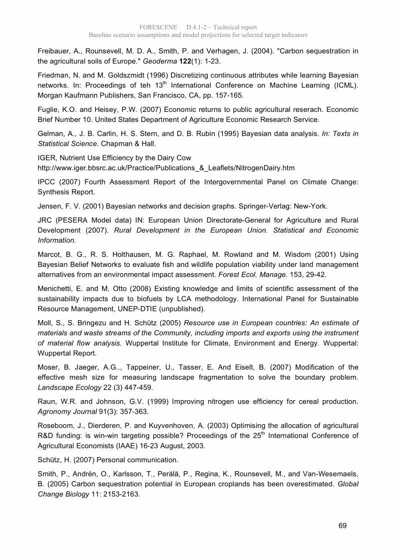
FORESCENE D.4.1-2 – Technical report
Baseline scenario assumptions and model projections for selected target indicators
69
Freibauer, A., Rounsevell, M. D. A., Smith, P. and Verhagen, J. (2004). "Carbon sequestration in
the agricultural soils of Europe." Geoderma 122(1): 1-23.
Friedman, N. and M. Goldszmidt (1996) Discretizing continuous attributes while learning Bayesian
networks. In: Proceedings of teh 13th International Conference on Machine Learning (ICML).
Morgan Kaufmann Publishers, San Francisco, CA, pp. 157-165.
Fuglie, K.O. and Heisey, P.W. (2007) Economic returns to public agricultural reserach. Economic
Brief Number 10. United States Department of Agriculture Economic Research Service.
Gelman, A., J. B. Carlin, H. S. Stern, and D. B. Rubin (1995) Bayesian data analysis. In: Texts in
Statistical Science. Chapman & Hall.
IGER, Nutrient Use Efficiency by the Dairy Cow
http://www.iger.bbsrc.ac.uk/Practice/Publications_&_Leaflets/NitrogenDairy.htm
IPCC (2007) Fourth Assessment Report of the Intergovernmental Panel on Climate Change:
Synthesis Report.
Jensen, F. V. (2001) Bayesian networks and decision graphs. Springer-Verlag: New-York.
JRC (PESERA Model data) IN: European Union Directorate-General for Agriculture and Rural
Development (2007). Rural Development in the European Union. Statistical and Economic
Information.
Marcot, B. G., R. S. Holthausen, M. G. Raphael, M. Rowland and M. Wisdom (2001) Using
Bayesian Belief Networks to evaluate fish and wildlife population viability under land management
alternatives from an environmental impact assessment. Forest Ecol. Manage. 153, 29-42.
Menichetti, E. and M. Otto (2008) Existing knowledge and limits of scientific assessment of the
sustainability impacts due to biofuels by LCA methodology. International Panel for Sustainable
Resource Management, UNEP-DTIE (unpublished).
Moll, S., S. Bringezu and H. Schütz (2005) Resource use in European countries: An estimate of
materials and waste streams of the Community, including imports and exports using the instrument
of material flow analysis. Wuppertal Institute for Climate, Environment and Energy. Wuppertal:
Wuppertal Report.
Moser, B. Jaeger, A.G.., Tappeiner, U., Tasser, E. And Eiselt, B. (2007) Modification of the
effective mesh size for measuring landscape fragmentation to solve the boundary problem.
Landscape Ecology 22 (3) 447-459.
Raun, W.R. and Johnson, G.V. (1999) Improving nitrogen use efficiency for cereal production.
Agronomy Journal 91(3): 357-363.
Roseboom, J., Dierderen, P. and Kuyvenhoven, A. (2003) Optimising the allocation of agricultural
R&D funding: is win-win targeting possible? Proceedings of the 25th International Conference of
Agricultural Economists (IAAE) 16-23 August, 2003.
Schütz, H. (2007) Personal communication.
Smith, P., Andrén, O., Karlsson, T., Perälä, P., Regina, K., Rounsevell, M., and Van-Wesemaels,
B. (2005) Carbon sequestration potential in European croplands has been overestimated. Global
Change Biology 11: 2153-2163.

70
Secretariat of the Convention on Biological Diversity (2006) Global Biodiversity Outlook 2.
Montreal.
Temple, H.J. and Terry, A. (Compilers). 2007. The Status and Distribution of European Mammals.
Luxembourg: Office for Official Publications of the European Communities.
UN, European Forest Sector Outlook Study 1960-2000-2020: Main Report (2005) UNECE, FAO.
UNECE FAO (2006) Forest Products Annual Market Review: Geneva Timber and Forest Study
Paper 21. United Nations, New York and Geneva.
Uusitalo, L. 2007. Advantages and challenges of Bayesian networks in environmental modelling.
Ecological Modelling 203: 312-318.
Van-Camp, L., Bujarrabal, B., Gentile, A.R., Jones, R.J.A., Montanarella, L., Olazabal, C., and
Selvaradjou, S-K. (2004) Reports of the technical working groups established under the Thematic
Strategy for Soil Protection. Volume III: Organic Matter. EUR 21319 EN/3, 872 pp. Office for Official
Publications of the European Communities, Luxembourg.
Weber, J.L., Spyropoulou, R., Soukup, T. and Páramo, F. (2008) Net Landscape Ecological
Potential of Europe and change 1990-2000. EEA.
World Database on Protected Areas, http://sea.unep-wcmc.org/wdbpa/


74
7 Appendix
7.1 Conditional Probability Tables (CPTs)
Cain (2001) defines a Bayesian Network as a ‘graphical tool for building decision support systems
to help make decisions under uncertain conditions’. The key phrase to focus on in this definition is
‘uncertain conditions’. As Cain points out, BNs were originally developed to allow the impact of
uncertainty in management to be accounted for. Using the tools decision makers could balance the
desirability of an outcome against the chance that the management option selected might fail. The
representation of a system in terms of a set of relationships that have probabilities associated with
them is at the heart of the Bayesian approach. An example of a simple BN is shown in Figure 34.
Figure 34: A simple BN
Source: after Cain 2001
If we think about the sorts of things that might influence agricultural yield, for example, then these
might include water supply and fertilizer applications. The amount of water applied to the crop
might, in turn, be influenced by such factors as soil type and the level of irrigation. Figure 34 shows
this diagrammatically. The key variables (that is the things that can change, such as yield, fertilizer
applications and soil type etc.) are shown as a set of boxes or nodes. The relationships between
the variables are shown as a set of arrows. These arrows simply set out the linkages between the
variables; they show what influences what. The arrows describe what we think the causal
relationships are within the system; notice that the arrows have a direction to express this idea of
causality.
In Figure 34 each of the nodes are shown as being able to take various states. Thus yield can be
‘good’ or ‘poor’, or soil type can be ‘sandy’ or ‘clay’. In the diagram, the nodes are represented by a
special type of box, called a ‘belief bar’, which we can use to express the probability that the
variable (node) is in a particular state, and how this might influence the other nodes to which it is
linked. At the moment no real probabilities have been assigned, and all the nodes show a 50:50
chance of being in a particular state. What the BN allows us to do is to assign probabilities to the
states for the different nodes to describe how we think the world actually works. The way we do this
is to build Conditional Probability Tables (CPT) for each node.

FORESCENE D.4.1-2 – Technical report
Baseline scenario assumptions and model projections for selected target indicators
75
Table 19: CPT for the Crop water Application Node
Table 19 shows the CPT for the node ‘Crop Water Application’ that is part of the network described
in Figure 34. Technically CPT is the contingency table of conditional probabilities15 stored at each
node, containing the probabilities of the node given each configuration of parent values. Clearly
when building a BN we do not have to confine ourselves to variables that have only two states. The
software can handle a number of discrete states or even continuous values.
15 The conditional probability of an event is the probability of the event occurring under certain given
conditions.

76
7.2 Values for model input nodes of the biodiversity, soils and landscape submodel for baseline scenarios 2000-2050
Table 20: Values for model input nodes of the biodiversity, soils and landscape submodel for baseline scenarios 2000-2050
Node Node Name Measurement 2000 2005 2010 2015 2020 2025 2030 2035 2040 2045 2050
85% 85% 78% 78% 69% 69% 58% 58% 47% 47% 36% NAES Agri-
environment
support
Probability for
CPT 15% 15% 22% 22% 31% 31% 42% 42% 53% 53% 64%
100% 90% 89% 88% 87% 86% 85% 84% 83% 82% 81% NCC Cross
compliance
Probability for
CPT 0% 10% 11% 12% 13% 14% 15% 16% 17% 18% 19%
% Efficiency
(mean)
28.0 28.3 28.6 28.8 29.1 29.4 29.7 30.0 30.3 30.6 30.9 NGTE Nutrient transfer
efficiency
(grassland)
% Efficiency
(stdev)
14.0 14.1 14.3 14.4 14.6 14.7 14.9 15.0 15.2 15.3 15.5
% Efficiency
(mean)
52.0 52.5 53.0 53.6 54.1 54.7 55.2 55.8 56.3 56.9 57.4 NATE Nutrient transfer
efficiency
(arable) % Efficiency
(stdev)
26.0 26.3 26.5 26.8 27.1 27.3 27.6 27.9 28.2 28.4 28.7
50.8% 49.5% 48.2% 46.9% 45.6% 44.3% 42.9% 41.4% 40.0% 38.5% 36.9% NFM Forest
management
Probability for
CPT 49.2% 50.5% 51.8% 53.1% 54.4% 55.7% 57.1% 58.6% 60.0% 61.5% 63.1%

FORESCENE D.4.1-2 – Technical report
Baseline scenario assumptions and model projections for selected target indicators
77
Table 21: Values for model input nodes of the biodiversity, soils and landscape submodel for baseline scenarios 2000-2050 (Continued 1)
Node Node Name Measurement 2000 2005 2010 2015 2020 2025 2030 2035 2040 2045 2050
Yield t ha-1
yr-1
(mean)
2.46 2.69 2.85 3.00 3.15 3.31 3.48 3.66 3.85 4.04 4.25 WBP9Y
Oilseed yield
Yield t ha-1
yr-1
(stdev)
0.16 0.17 0.18 0.19 0.20 0.21 0.22 0.24 0.25 0.26 0.27
Yield t ha-1
yr-1
(mean)
5.25 5.40 5.62 5.79 5.98 6.16 6.35 6.55 6.76 6.97 7.19 WBP10Y
Wheat yield
Yield t ha-1
yr-1
(stdev)
0.33 0.34 0.35 0.36 0.38 0.39 0.40 0.41 0.42 0.44 0.45
Yield t ha-1
yr-1
(mean)
2.43 2.45 2.55 2.60 2.66 2.71 2.77 2.82 2.88 2.94 3.00 WBP11Y
Grains yield
Yield t ha-1
yr-1
(stdev)
0.23 0.23 0.24 0.25 0.25 0.26 0.26 0.27 0.27 0.28 0.28
Yield t ha-1
yr-1
(mean)
54.24 57.32 60.98 61.60 62.22 62.85 63.49 64.13 64.78 65.43 66.10 WBP12Y
Sugar beet yield
Yield t ha-1
yr-1
(stdev)
3.51 3.71 3.95 3.99 4.03 4.07 4.11 4.15 4.19 4.23 4.28
Yield t ha-1
yr-1
(mean)
4.17 4.26 4.37 4.45 4.54 4.63 4.71 4.80 4.90 4.99 5.09 WBP13Y
Rice yield
Yield t ha-1
yr-1
(stdev)
0.18 0.18 0.18 0.19 0.19 0.19 0.20 0.20 0.21 0.21 0.21
WBP14Y Pasture yield for
beef, mutton
and milk
Yield t ha-1
yr-1
(mean)
0.32 0.30 0.30 0.30 0.30 0.30 0.30 0.30 0.30 0.30 0.30

78
Table 22: Values for model input nodes of the biodiversity, soils and landscape submodel for baseline scenarios 2000-2050 (Continued 2)
Node Node Name Measurement 2000 2005 2010 2015 2020 2025 2030 2035 2040 2045 2050
Hectares 17,059,
563
17,490,
338
17,931,
991
18,384,
797
18,849,
036
19,324,
997
19,812,
978
20,313,
280
20,826,
216
21,352,
104
21,891,
272
NARA EU artificial
area
Hectares
(stdev)
852,97
8
874,51
7
896,60
0
919,24
0
942,45
2
966,25
0
990,64
9
1,015,6
64
1,041,3
11
1,067,6
05
1,094,5
64
Hectares 178,51
7,000
172,37
6,000
167,20
4,720
162,18
8,578
157,32
2,921
152,60
3,233
148,02
5,136
143,58
4,382
139,27
6,851
135,09
8,545
131,04
5,589
WBP1 EU agricultural
area
Hectares
(stdev)
8,925,8
50
8,618,8
00
8,360,2
36
8,109,4
29
7,866,1
46
7,630,1
62
7,401,2
57
7,179,2
19
6,963,8
43
6,754,9
27
6,552,2
79
Hectares 164,17
0,000
166,44
1,000
169,79
6,557
173,21
9,765
176,71
1,986
180,27
4,613
183,90
9,065
187,61
6,790
191,39
9,265
195,25
7,996
199,19
4,523
LF EU forest area
Hectares
(stdev)
8,208,5
00
8,322,0
50
8,489,8
28
8,660,9
88
8,835,5
99
9,013,7
31
9,195,4
53
9,380,8
39
9,569,9
63
9,762,9
00
9,959,7
26
54% 54% 46% 42% 38% 34% 31% 27% 24% 21% 19%
27% 27% 32% 35% 37% 40% 42% 44% 46% 49% 50%
NGHS Grassland
habitat status
Probability for
CPT
19% 19% 22% 23% 25% 26% 27% 28% 29% 30% 31%
41% 41% 27% 22% 17% 13% 10% 7% 5% 4% 3%
33% 33% 37% 38% 37% 37% 35% 34% 32% 30% 28%
NFHS Forest habitat
status
Probability for
CPT
26% 26% 36% 41% 46% 50% 55% 59% 62% 66% 69%
56% 56% 42% 35% 28% 22% 17% 12% 9% 6% 4%
37% 37% 43% 44% 44% 42% 39% 35% 31% 26% 21%
NBHS Bogs and mires
habitat status
Probability for
CPT
8% 8% 15% 21% 28% 35% 44% 53% 61% 68% 75%

FORESCENE D.4.1-2 – Technical report
Baseline scenario assumptions and model projections for selected target indicators
79
Table 23: Values for model input nodes of the biodiversity, soils and landscape submodel for baseline scenarios 2000-2050 (Continued 3)
Node Node Name Measurement 2000 2005 2010 2015 2020 2025 2030 2035 2040 2045 2050
37.0% 37% 28% 23% 19% 15% 12% 9% 6% 5% 3%
40.0% 40% 36% 32% 29% 24% 20% 16% 13% 10% 8%
NHHS Heath and
scrub status
Probability for
CPT
23.0% 23% 36% 44% 52% 60% 68% 75% 80% 85% 89%
10.3% 10% 16% 20% 24% 29% 33% 38% 43% 47% 52%
47.0% 47% 32% 25% 20% 15% 11% 8% 6% 4% 3%
NSHS Sclerophyllus
scrub status
Probability for
CPT
43.3% 43% 52% 55% 56% 56% 55% 54% 51% 48% 45%
34.3% 34% 20% 15% 11% 8% 6% 4% 3% 2% 1%
45.3% 45% 53% 55% 56% 56% 56% 55% 54% 52% 51%
NAHS Aquatic habitat
status
Probability for
CPT
20.3% 20% 27% 30% 33% 36% 39% 41% 43% 45% 48%
35.0% 35.0% 29% 26% 23% 20% 18% 15% 13% 11% 9%
36.0% 36.0% 33% 31% 29% 27% 24% 22% 19% 17% 15%
NMSS Mammal
species status
Probability for
CPT
29.0% 29.0% 38% 43% 48% 53% 58% 63% 68% 72% 76%
28.0% 28.0% 20% 16% 12% 9% 7% 5% 3% 2% 2%
43.0% 43.0% 42% 38% 34% 29% 24% 20% 16% 12% 10%
NPSS Plant species
status
Probability for
CPT
29.0% 29.0% 38% 46% 54% 62% 69% 76% 81% 85% 89%
48.0% 46.6% 45.0% 43.5% 42.1% 40.6% 39.2% 37.8% 36.4% 35.0% 33.6% NBSS Bird species
status
Probability for
CPT 52.0% 53.6% 55.0% 56.5% 57.9% 59.4% 60.8% 62.2% 63.6% 65.0% 66.4%
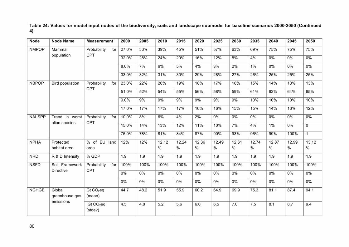
80
Table 24: Values for model input nodes of the biodiversity, soils and landscape submodel for baseline scenarios 2000-2050 (Continued
4)
Node Node Name Measurement 2000 2005 2010 2015 2020 2025 2030 2035 2040 2045 2050
27.0% 33% 39% 45% 51% 57% 63% 69% 75% 75% 75%
32.0% 28% 24% 20% 16% 12% 8% 4% 0% 0% 0%
8.0% 7% 6% 5% 4% 3% 2% 1% 0% 0% 0%
NMPOP Mammal
population
Probability for
CPT
33.0% 32% 31% 30% 29% 28% 27% 26% 25% 25% 25%
23.0% 22% 20% 19% 18% 17% 16% 15% 14% 13% 13%
51.0% 52% 54% 55% 56% 58% 59% 61% 62% 64% 65%
9.0% 9% 9% 9% 9% 9% 9% 10% 10% 10% 10%
NBPOP Bird population Probability for
CPT
17.0% 17% 17% 17% 16% 16% 15% 15% 14% 13% 12%
10.0% 8% 6% 4% 2% 0% 0% 0% 0% 0% 0%
15.0% 14% 13% 12% 11% 10% 7% 4% 1% 0% 0
NALSPP Trend in worst
alien species
Probability for
CPT
75.0% 78% 81% 84% 87% 90% 93% 96% 99% 100% 1
NPHA Protected
habitat area
% of EU land
area
12% 12% 12.12
%
12.24
%
12.36
%
12.49
%
12.61
%
12.74
%
12.87
%
12.99
%
13.12
%
NRD R & D Intensity % GDP 1.9 1.9 1.9 1.9 1.9 1.9 1.9 1.9 1.9 1.9 1.9
100% 100% 100% 100% 100% 100% 100% 100% 100% 100% 100%
0% 0% 0% 0% 0% 0% 0% 0% 0% 0% 0%
NSFD Soil Framework
Directive
Probability for
CPT
0% 0% 0% 0% 0% 0% 0% 0% 0% 0% 0%
Gt CO2eq
(mean)
44.7 48.2 51.9 55.9 60.2 64.9 69.9 75.3 81.1 87.4 94.1 NGHGE Global
greenhouse gas
emissions Gt CO2eq
(stdev)
4.5 4.8 5.2 5.6 6.0 6.5 7.0 7.5 8.1 8.7 9.4
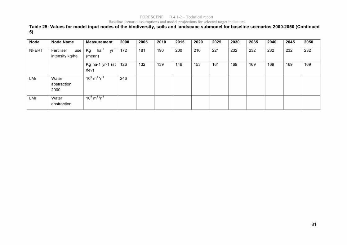
FORESCENE D.4.1-2 – Technical report
Baseline scenario assumptions and model projections for selected target indicators
81
Table 25: Values for model input nodes of the biodiversity, soils and landscape submodel for baseline scenarios 2000-2050 (Continued 5)
Node Node Name Measurement 2000 2005 2010 2015 2020 2025 2030 2035 2040 2045 2050
Kg ha-1
yr-1
(mean)
172 181 190 200 210 221 232 232 232 232 232 NFERT Fertiliser use
intensity kg/ha
Kg ha-1 yr-1 (st
dev)
126 132 139 146 153 161 169 169 169 169 169
LMr Water
abstraction
2000
109 m
3 yr-1
246
LMr Water
abstraction
109 m
3 yr-1

82
Table 26: List of nodes values with value used in place of normal distribution in baseline model test
Node Node Name Measurement 2000 2005 2010 2015 2020 2025 2030 2035 2040 2045 2050
NGTE Nutrient transfer
efficiency
(grassland)
% Efficiency
(mean)
28.0 28.3 28.6 28.8 29.1 29.4 29.7 30.0 30.3 30.6 30.9
NATE Nutrient transfer
efficiency
(arable)
% Efficiency
(mean)
52.0 52.5 53.0 53.6 54.1 54.7 55.2 55.8 56.3 56.9 57.4
WBP9Y
Oilseed yield
Yield t ha-1
yr-1
(mean)
2.46 2.69 2.85 3.00 3.15 3.31 3.48 3.66 3.85 4.04 4.25
WBP10Y
Wheat yield
Yield t ha-1
yr-1
(mean)
5.25 5.40 5.62 5.79 5.98 6.16 6.35 6.55 6.76 6.97 7.19
WBP11Y
Grains yield
Yield t ha-1
yr-1
(mean)
2.43 2.45 2.55 2.60 2.66 2.71 2.77 2.82 2.88 2.94 3.00
WBP12Y
Sugar beet yield
Yield t ha-1
yr-1
(mean)
54.24 57.32 60.98 61.60 62.22 62.85 63.49 64.13 64.78 65.43 66.10
WBP13Y
Rice yield
Yield t ha-1
yr-1
(mean)
4.17 4.26 4.37 4.45 4.54 4.63 4.71 4.80 4.90 4.99 5.09

FORESCENE D.4.1-2 – Technical report
Baseline scenario assumptions and model projections for selected target indicators
83
Node Node name Measurement 2000 2005 2010 2015 2020 2025 2030 2035 2040 2045 2050
NARA EU artificial
area
Hectares 17,059,563 17,490,338 17,931,991 18,384,797 18,849,036 19,324,997 19,812,978 20,313,280 20,826,216 21,352,104 21,891,272
WBP1 EU
agricultural
area
Hectares 178,517,000 172,376,000 167,204,720 162,188,578 157,322,921 152,603,233 148,025,136 143,584,382 139,276,851 135,098,545 131,045,589
LF EU forest
area
Hectares 164,170,000 166,441,000 169,796,557 173,219,765 176,711,986 180,274,613 183,909,065 187,616,790 191,399,265 195,257,996 199,194,523
NGHGE Global
greenhouse
gas
emissions
Gt CO2
equivalent
(mean)
44.7 48.2 51.9 55.9 60.2 64.9 69.9 75.3 81.1 87.4 94.1
NFERT Fertiliser use
intensity
kg/ha
Kg ha-1
yr-1
(mean)
172 181 190 200 210 221 232 232 232 232 232
84
7.3 Definitions of forest land from Eurostat Forestry Statistics 2007
Forest is defined as land with tree crown cover (or equivalent stocking level) of more than 10%
and area of more than 0.5 ha. The trees should be able to reach a minimum height of 5 m at
maturity in situ. It may consist of either closed forest formations, where trees of various storeys
and undergrowth cover a high proportion of the ground, or of open forest formations, with a
continuous vegetation cover, in which tree crown cover exceeds 10% of the area. Young natural
stands and all plantations established for forestry purposes that have yet to reach a crown
density of 10%, or a tree height of 5 m, are included under forest. This is because they are
areas that normally form part of the forest area, that are temporarily unstocked as a result of
human intervention or natural causes, but that are expected to revert to forest.
Other Wooded Land is land either with a tree crown cover (or equivalent stocking level) of 5-
10% of trees able to reach a height of 5 m at maturity in situ, or a crown cover (or equivalent
stocking level) of more than 10% of trees not able to reach a height of 5 m at maturity in situ
(e.g. dwarf or stunted trees) and shrub or bush cover.
FOWL is the total of Forest and Other Wooded Land.