Embed Size (px)
Citation preview
Project Number: BS2 0804
Authentication Schemes based on Physically Unclonable Functions
A Major Qualifying Project Report
submitted to the Faculty
of the
WORCESTER POLYTECHNIC INSTITUTE
in partial ful�llment of the requirements for the
Degree of Bachelor of Science
by
Matthew D. Dailey
Ilan Shomorony
Date: April 30, 2009
Approved:
Professor Berk Sunar, Major Advisor
Professor William J. Martin, Major Advisor
Abstract
In this project we investigate di�erent hardware authentication schemes based on Phys-ically Unclonable Functions. We start by analyzing the concepts of a fuzzy extractorand a secure sketch from an information-theoretic perspective. We then present a hard-ware implementation of a fuzzy extractor which uses the code o�set construction withBCH codes. Finally, we propose a new cryptographic protocol for PUF authenticationbased upon polynomial interpolation using Sudan's list-decoding algorithm. We providepreliminary results into the feasibility of this protocol, by looking at the practicality of�nding a polynomial that can be assigned as a cryptographic key to each device.
Contents
1 Introduction 3
2 Physically Unclonable Functions 42.1 Mathematical Model . . . . . . . . . . . . . . . . . . . . . . . . . . . . . 5
2.1.1 Same neighborhood with high probability . . . . . . . . . . . . . . 52.1.2 Same output with high probability . . . . . . . . . . . . . . . . . 6
3 Error-Correcting Codes 73.1 Terminology . . . . . . . . . . . . . . . . . . . . . . . . . . . . . . . . . . 73.2 Linear Codes . . . . . . . . . . . . . . . . . . . . . . . . . . . . . . . . . 83.3 BCH Codes . . . . . . . . . . . . . . . . . . . . . . . . . . . . . . . . . . 9
3.3.1 Encoding . . . . . . . . . . . . . . . . . . . . . . . . . . . . . . . 93.3.2 Decoding . . . . . . . . . . . . . . . . . . . . . . . . . . . . . . . 10
3.4 Reed-Solomon Codes . . . . . . . . . . . . . . . . . . . . . . . . . . . . . 113.4.1 Code description . . . . . . . . . . . . . . . . . . . . . . . . . . . 113.4.2 Alternative look at Reed-Solomon codes . . . . . . . . . . . . . . 11
4 Fuzzy Extractors and PUFs 134.1 Basic Ideas . . . . . . . . . . . . . . . . . . . . . . . . . . . . . . . . . . 134.2 Preliminary De�nitions . . . . . . . . . . . . . . . . . . . . . . . . . . . . 144.3 Secure Sketches . . . . . . . . . . . . . . . . . . . . . . . . . . . . . . . . 154.4 The Code-O�set construction . . . . . . . . . . . . . . . . . . . . . . . . 174.5 Fuzzy Extractors . . . . . . . . . . . . . . . . . . . . . . . . . . . . . . . 224.6 Hash Functions . . . . . . . . . . . . . . . . . . . . . . . . . . . . . . . . 244.7 Overall design of fuzzy extractors . . . . . . . . . . . . . . . . . . . . . . 26
5 Hardware implementation of Fuzzy Extractors 285.1 BCH codes and Fuzzy Extractors . . . . . . . . . . . . . . . . . . . . . . 285.2 Hardware architecture for a BCH decoder . . . . . . . . . . . . . . . . . 29
5.2.1 Basic steps in BCH decoding . . . . . . . . . . . . . . . . . . . . . 295.2.2 Syndrome Computation . . . . . . . . . . . . . . . . . . . . . . . 305.2.3 Finding the Error-Locator polynomial . . . . . . . . . . . . . . . . 315.2.4 The Berlekamp-Massey Algorithm . . . . . . . . . . . . . . . . . . 345.2.5 Correcting errors . . . . . . . . . . . . . . . . . . . . . . . . . . . 42
5.3 BCH Decoder Implementation Results . . . . . . . . . . . . . . . . . . . 44
1
6 A new approach to PUF-based hardware authentication 486.1 Polynomial as the secret . . . . . . . . . . . . . . . . . . . . . . . . . . . 486.2 Polynomial Interpolation . . . . . . . . . . . . . . . . . . . . . . . . . . . 496.3 Lagrange Interpolation . . . . . . . . . . . . . . . . . . . . . . . . . . . . 50
6.3.1 Restrictions on Lagrange Interpolation . . . . . . . . . . . . . . . 516.4 Polynomial interpolation �with lies� . . . . . . . . . . . . . . . . . . . . . 516.5 Sudan's algorithm . . . . . . . . . . . . . . . . . . . . . . . . . . . . . . . 54
6.5.1 Sudan's algorithm procedure [17] . . . . . . . . . . . . . . . . . . 556.5.2 The polynomial Q(x, y) . . . . . . . . . . . . . . . . . . . . . . . . 566.5.3 Polynomially many solutions . . . . . . . . . . . . . . . . . . . . . 586.5.4 Factoring Polynomials . . . . . . . . . . . . . . . . . . . . . . . . 586.5.5 Implementing Sudan's Algorithm . . . . . . . . . . . . . . . . . . 59
7 Protocol 627.1 Protocol Assumptions . . . . . . . . . . . . . . . . . . . . . . . . . . . . 627.2 Protocol design iterations . . . . . . . . . . . . . . . . . . . . . . . . . . 63
7.2.1 Initial Protocol . . . . . . . . . . . . . . . . . . . . . . . . . . . . 637.2.2 Hashed output . . . . . . . . . . . . . . . . . . . . . . . . . . . . 637.2.3 Sudan's algorithm for recovering from noise . . . . . . . . . . . . 647.2.4 Challenge-dependent hashed coe�cients . . . . . . . . . . . . . . 64
7.3 Existence of low-degree polynomial . . . . . . . . . . . . . . . . . . . . . 657.3.1 The particular case of a zero-degree polynomial . . . . . . . . . . 657.3.2 Back to the original problem . . . . . . . . . . . . . . . . . . . . . 667.3.3 Coding-theory techniques to estimate probability . . . . . . . . . 67
8 Conclusion 728.1 Future Work . . . . . . . . . . . . . . . . . . . . . . . . . . . . . . . . . . 73
Bibliography 75
Appendix 77
A Selected proofs 77
B Hardware Complexity 79B.1 Average number of nonzero coe�cients for elements of GF (2m) . . . . . . 79B.2 Reducing the complexity of Syndrome computation . . . . . . . . . . . . 79B.3 Gate count for Inverter block . . . . . . . . . . . . . . . . . . . . . . . . 81B.4 Gate count for Chien's Search block . . . . . . . . . . . . . . . . . . . . . 81
C Sudan's algorithm maple source code 82
2
Chapter 1
Introduction
In today's world, the concern about piracy and counterfeit products is constantly increas-ing. The same advances that supply us with new technologies provide counterfeiters witha way of reverse-engineering and reproducing them. As we move into an era where we relyon small devices, such as cell-phones, credit cards and RFIDs, to store sensitive personalinformation and to grant us access to bank accounts, medical records and private areas,the importance of �ghting counterfeiting becomes even more evident.
Research for ways of assigning digital �ngerprints to devices, which allow for easyauthentication and the detection of cloned devices has been receiving much attention.One of the most interesting methods of hardware �ngerprinting, proposed in [14], isthe idea of Physically Unclonable Functions (PUFs). These functions make use of verysensitive physical properties of a device in order to assign it a unique identi�er, makingthe task of producing an identical device much harder.
A great deal of e�ort has been put into developing ways of using these PUFs toprovide reliable authentication of devices. Most of the schemes proposed so far rely oncollecting challenge-response pairs that are unique to each PUF device. However, thesame properties that make PUFs attractive for cryptographic applications make themhard to deal with. Due to the high sensitivity to physical parameters, the responses of aPUF are naturally noisy. In this project, we examine some of the ways of handling thisnoise and propose a new method which presents a possible improvement in the securityof the authentication protocol.
In chapter 2, we introduce the idea of a physically unclonable function which mapschallenges to responses that depend highly of the physical properties of each device.Small variations between devices allow for a unique identi�er to be assigned to eachdevice, which can serve as a cryptographic key. In chapter 3, we introduce the conceptof an error-correcting code which allows for messages sent over a noisy channel to becorrectly received. We describe BCH codes and their special case, Reed Solomon Codes.In chapter 4, we analyze the known methods of fuzzy extractors and secure sketches as away to recover from the noise associated with the responses of a PUF device. In chapter5, we provide an implementation of a fuzzy extractor in hardware that aims at areae�ciency. In chapter 6, we introduce a new methodology to assign a key to each PUFdevice based upon polynomial interpolation and present Sudan's list decoding algorithmas a way to extract the key from the noisy outputs of the device. Finally, in chapter 7,we present a protocol which is based upon this method, and analyze its feasibility.
3
Chapter 2
Physically Unclonable Functions
The term Physically Unclonable Function, or PUF, is used by scientists and engineers torefer to a practical device or process with a measurable output that strongly depends uponphysical parameters. These �functions� are usually embodied in a hardware structure,such as a chip or a circuit board, and they obtain their �unclonability� from the fact thattheir outcomes depend on very sensitive physical properties, such as the length of wiresor silicon doping levels, which cannot be precisely controlled in a manufacturing process.
In this report, we will be mostly concerned with a particular kind of PUFs, thechallenge-response PUFs. These PUFs return a physically-dependent response r whengiven a challenge c. An important property of challenge-response PUFs is that when twodevices from the same manufacturing process are given the same input, and are underthe same external in�uences � temperature, pressure, magnetic �elds, etc. � theiroutputs may di�er. These di�erences are not intended, but are inherent in the nature ofmass-produced devices. Therefore, if a PUF exploits a physical parameter with enoughvariability in such a way that the mapping between challenges and responses is uniqueto each device, it can be used to authenticate or uniquely identify that device.
Due to the high level of sensitivity of the physical parameters involved, it is consideredinfeasible for a person, when given the distribution on the responses of a speci�c PUFdevice, to fabricate another device which will produce identical responses. However, it isnot considered infeasible for someone to model the responses of a speci�c PUF and usea di�erent device that simply maps inputs to outputs in the same way, possibly usingsoftware.
An assumption that can be made about PUFs is that their internal workings behaveas a �black box� and only their public output can be measured. For example, if a devicewere to receive ten challenges it would produce ten responses. If the device were torespond (output) with a hash of these ten responses, then it is assumed that the actualresponse to each of the ten inputs is part of the internal workings of the black box. Anadversary would only have access to the hash of these responses. This assumption isjusti�ed by the fact that if an adversary opens the device to view the responses of thecircuit, the physical parameters of the circuit will be altered and it will consequentlyproduce di�erent responses. Putting the device back together does not guarantee thedevice will produce the same outputs as before.
From the cryptographic perspective, PUF devices are attractive since the di�erentoutputs among these otherwise identical devices can be used to identify and authenticate
4
a particular device. Moreover, this can be accomplished without explicitly storing anyauthenticating information on the device, such as a cryptographic key. Other authen-tication schemes such as public-key cryptography require the device's private key to beexplicitly stored somewhere in the memory on the device. An authentication schemeutilizing PUFs can use the unique physical properties of each device to generate a keyevery time the device is prompted with challenges. If an adversary attempted to learnthis key through an active attack, the physical properties of the device would change andthis key would become unusable.
Example 2.1.We now follow [6] to present the delay-based PUF. A delay-based PUF receives a challengec ∈ {0, 1}k and responds with r ∈ {0, 1}. Upon receiving a challenge, a pulse generatorgenerates a signal which then splits and travels down two wires, which we will refer toas the top wire and the bottom wire. Each wire passes through k switches serially. Theoutput of one switch is the input to the next switch. Both wires are then connected toan arbiter which outputs a 1 if the signal on the top wire arrives �rst, a 0 if the signalon the bottom wire arrives �rst, or if the di�erence in arrival times is below the arbiter'ssensitivity level, it outputs 0 or 1 uniformly at random. When the kth challenge bit isa 0, the kth switch allows the two signals to pass through in a straight path and remainon the same wire. Otherwise, if the kth challenge bit is a 1, the kth switch switches thesignal, and the signal which was on the top wire is now on the bottom wire and the signalthat was on the bottom wire is now on the top wire.
These wires are designed to have equal length. However, the process variations lead tolength variations and to di�erent time delays for each signal. These delays are dependentupon the challenge received, and upon the speci�c circuit. Two identically producedcircuits will have di�erent length wires and will respond di�erently to certain challenges.It is these di�erences which can be used to authenticate the device.
2.1 Mathematical Model
We will use two slightly di�erent mathematical models for the PUF function. We will �rstdescribe a PUF which will respond from a set of responses which are in some neighborhoodof each other when given the same challenge. Then we consider the case where, for eachchallenge, the PUF produces an identical output with high probability.
2.1.1 Same neighborhood with high probability
In order to apply the concept of secure sketches to PUFs (see Section 4.3) we need tode�ne the concept of proximity, or distance between the possible outputs of the PUF.A secure sketch can take advantage of a PUF which, when given the same challenge c,outputs responses which are a small distance away from each other (see [3] and [4]).
We formalize this as follows. Let F be a �nite �eld with q elements and let Y be aprobability space. We assume our co-domain F is a metric space with distance functiondis . We let Rc be a set of responses to challenge a c ∈ F such that dis(ri, rj) ≤ t for all
5
ri, rj in Rc. We now de�ne our PUF function as a map
PUF : F× Y → F
such thatPUF (c, y)y←Y ∈ Rc with probability at least 1− ε (2.1)
Property (2.1) formalizes the de�nition of closeness of the outputs to the same input, orthe expected neighborhood.
2.1.2 Same output with high probability
In order to introduce the idea of PUF authentication through polynomial interpolation(see Section 6.1), we modify the previous de�nition slightly. We let F be a �nite �eldwith q elements and Y be a probability space. Then we assume that there exists a highlynonlinear function
f : F→ F
We now model our PUF function as
PUF : F× Y → F
wherePUF (c, y)y←Y = f(c) with probability at least 1− ε (2.2)
Property (2.2) states that with y ranging over all of Y , f(c) is the output with prob-ability at least 1− ε.
We will refer to f(c) as the expected output of the PUF to challenge c. Abusingnotation, we will refer to PUF (c, y)y←Y as PUF (c). We therefore have that for eachc ∈ F, the output of the PUF function to challenge c is PUF (c) with probability at least1− ε.
6
Chapter 3
Error-Correcting Codes
Coding theory primarily addresses the problem of sending information over a channelwhich may distort the information. In a communication system, we assume the existenceof two parties, a transmitter and a receiver. In order to assure that the information iscorrectly received, the transmitter and the receiver agree beforehand on a set of rules,called a Code, which, if followed, will make the transmitted message more resilient tonoise. More speci�cally, the two parties agree on a subset of all transmittable messages,the codewords, which can be sent over the channel.
The theory of error-correcting codes deals with the detection and correction of errorsin the received information and with the design of codes that will increase the chances ofsuccessful information recovery from a noisy channel.
3.1 Terminology
Working over the binary alphabet, we call a 0 or 1 a digit, and we call a sequence ofdigits a word. We will only consider consider block codes, in which all words have thesame length. We letM be a metric space with dimension n = log2 |M|, which consistsof all binary words of length n. A code C is simply a collection of words, i.e. a subset ofM. A word that belongs to the code is called a codeword. We denote the dimension ofC by k = log2 |C|, when C is a subspace ofM.
More generally, if the alphabet F has size q, we refer to the dimension of the code ask = logq |C| and the dimension of the space as n = logq |M|. We de�ne the information
rate of the code to be kn.
The space M has a distance function dis : M×M → [0,+∞). We will mostly beinterested in the Hamming distance.
De�nition 3.1. Hamming distance: If w,w′ ∈ M = Fn, then dis (w,w′) is the numberof positions in which w and w′ di�er. Similarly, the Hamming weight of w is the numberof nonzero positions in w, or simply dis (w, 0).
De�nition 3.2. Minimum distance: The minimum distance d of a code is given by:
d = min {dis (w,w′) : w,w′ ∈ C,w 6= w′}
7
In general, a k-dimensional code which is de�ned over an n-dimensional metric space(and therefore has block size n), and with a minimum distance d is referred to as a(n,M, d)q code, where q is the size of the alphabet F and M = |C|.
Recovering the transmitted codeword
It is assumed that the errors on a transmission channel are somewhat unlikely (withprobability less than 1
2). Therefore the problem of recovering the transmitted codeword
can be reduced to �nding the codeword closest to the received word. In other words, anerror-correcting scheme is usually concerned with �nding the (preferably unique) code-word within a speci�ed distance from the received word. The maximum distance (ornumber of errors) from the received word within which we are assured to have a uniquecodeword is the error-correction bound t of the code.
The maximum likelihood decoding problem, also known as the nearest codeword prob-lem, is the problem of �nding the nearest codeword to the received word. This is oftenused when a large number of errors is considered less likely. This is a generalization of thet-error correction scheme since a received element s, which is at distance most t from acodeword, will be decoded into the codeword. However, if s is at a distance greater thant from a codeword, this scheme will return the nearest codeword, or one of the nearestcodewords.
The p-reconstruction problem also known as the list-decoding problem also generalizesthe t-error correction. In this problem we are given an element s, and we �nd all codewordswhich are within a distance p of s. In other words, we �nd all codewords that are ina moderate-sized n dimensional Hamming sphere around the received element s. Thedecoding is considered successful if the transmitted element is a member of the list.
3.2 Linear Codes
In this report, we will mostly deal with linear codes and not all statements hold for non-linear codes. A linear code is a code which is closed under the addition of codewords,
u, v ∈ C ⇒ (u+ v) ∈ C ,
and scalar multiplication, if q > 2. A linear code must contain the zero word. This isshown by adding a codeword c to itself |F| − 1 times. When the codewords are from thebinary �eld, a codeword added to itself is the zero codeword. The distance of a linear codeC is the minimum weight of any non-zero codeword in C. This is a standard result whichis shown by letting the minimum weight of a non-zero codeword be ω. Then, assume thatthere are two codewords, u, v ∈ C : φ = dis (u, v) < ω. Since C is a linear code, u− v is acodeword which has weight less than ω. Therefore we must have u− v = 0 which impliesu = v.
To refer to linear codes, it is common to use the form [n, k, d]q, where k is the dimensionof C.
8
Hamming bound [7]
If C is a code of length n and minimum distance d = 2t+ 1 or d = 2t+ 2 then
|C|((
n
0
)+
(n
1
)+ ...+
(n
t
))≤ 2n
A perfect code is a code in which the Hamming bound is met. In other words, for eachelement w in our metric space M, there exists a unique codeword c ∈ C such thatdis (w, c) ≤ t, meaning there exists a unique codeword within the error-correcting boundof the code.
We now introduce the two types of error-correcting codes used throughout this report:the BCH codes, and their non-binary special case, the famous Reed-Solomon codes.
3.3 BCH Codes
BCH codes are a large class of powerful error-correcting codes, invented in 1959 by Hoc-quenghem, and independently in 1960 by Bose and Ray-Chaudhuri. The great advantageof BCH codes is that given a block size n = qm−1, for any integer m, one can successfullybuild an [n, k, 2t+ 1]q code for any error-correction bound t ≤ qm−1 − 1, with dimensionk ≥ n−mt (see [15]). In general, even though BCH codes can be de�ned for non-binaryalphabets (q > 2), it is in the binary case that they �nd their largest applicability. Amongthe non-binary examples, we have the ubiquitous Reed Solomon codes, analyzed more indepth in Section 3.4.
Formally, BCH codes are cyclic polynomial codes, constructed as follows. For a givenn = qm − 1 block size, we can build a linear code with minimum distance d = 2t+ 1, bytaking a primitive element α of GF (qm) and de�ning the code generator polynomial as:
g(x) = LCM (φ1(x), φ2(x), φ3(x), ..., φ2t(x)) (3.1)
where φi(x) is the minimal polynomial of αi over GF (q). To show that this generates acode with minimum distance d = 2t + 1 we refer to Appendix A.3, where we prove thisfor the special case of Reed-Solomon codes. The proof for general BCH codes is similar[13].
3.3.1 Encoding
The encoding process for a BCH code takes a k-tuple with symbols from GF (q) andadds d− 1 = 2t parity check digits. Let us suppose that we have our k-symbol message,represented by the following polynomial:
a(x) = a0 + a1x+ ...+ ak−1xk−1
Then we multiply a(x) by xd−1 and use the division algorithm to write:
xd−1a(x) = g(x)c(x) + b(x)⇒ xd−1a(x)− b(x) = g(x)c(x)
Since xd−1a(x)− b(x) is shown to be a multiple of the generator polynomial it must be acodeword.
9
3.3.2 Decoding
Our received codeword r(x), an nth-degree polynomial, can be expressed as r(x) = v(x)+e(x), where v(x) was the transmitted codeword and e(x) is the error vector, caused bythe noise in the channel.Since v(x) is a codeword, we know that v(αi) = 0 for i = 1, 2, ..., d− 1, and therefore wehave
r(αi) = e(αi) i = 1, 2, ..., d− 1
This allows us to compute the d-1 syndromes of the received message to be:
S1 = r(α) = ej1αj1 + ej2α
j2 + ...+ ejταjτ
S2 = r(α2) = ej1α2j1 + ej2α
2j2 + ...+ e2jτα2jτ
...
Sd−1 = r(αd−1) = ej1α(d−1)j1 + ej2α
(d−1)j2 + ...+ ejτα(d−1)jτ
where τ is the number of errors that actually occurred.We then de�ne the error-locator polynomial to be:
σ(x) = (1− αj1x)(1− αj2x)...(1− αjτx) =
= 1 + σ1x+ ...+ στxτ (3.2)
Clearly, if we have the error-locator polynomial, the error locations can easily be foundby �nding the roots of σ(x). Then, if α−i is a root of σ(x), then there was an error atthe ith position. The coe�cients in (3.2) can be found from the d−1 syndromes by usingthe Berlekamp-Massey algorithm (see Section 5.2.4).
Once we have the error-locator polynomial all we have to do is �nd its roots andcalculate their inverses in order to �nd the locations in our received vector r(x) whereerrors have occurred. At this point, if we are in the binary case, correcting the errors istrivial. We simply �ip the bits at the location of the errors.
In the non-binary case, we still need to determine what the actual errors were. Inorder to do that we �rst de�ne the error-evaluator polynomial to be
Z(x) = σ(x)S(x) (mod x2t+1) (3.3)
where S(x) is the 2tth-degree polynomial formed by looking at each of the syndromes Sias the coe�cient of xi. Then we can show that the error eji at the j
thi location is given
by
eji =Z(α−ji)
τ∏a=1,a6=i
(1 + αaα−ji)
. (3.4)
Finally, one can simply subtract each of the errors eji from the jthi coe�cient of r(x) in
order to obtain v(x).
10
3.4 Reed-Solomon Codes
Invented in 1959 by Irving Reed and Gustave Solomon, the Reed-Solomon codes areprobably the most ubiquitous type of error-control codes. The fact that they achievethe Singleton Bound (see Section 7.3.3, Equation (7.5)) allied to their robustness againstburst errors made them the code of choice in several applications, ranging from compactdiscs to the transmission system of the Voyager spacecraft. However, the discovery thatReed-Solomon codes can be thought of as a special non-binary case of BCH codes is dueto Gorenstein and Zierler, in 1961. Because of that, the same encoding and decodingsteps described in the previous section hold for Reed-Solomon codes.
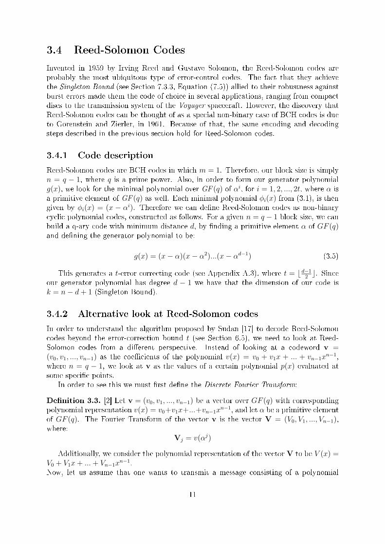
3.4.1 Code description
Reed-Solomon codes are BCH codes in which m = 1. Therefore, our block size is simplyn = q − 1, where q is a prime power. Also, in order to form our generator polynomialg(x), we look for the minimal polynomial over GF (q) of αi, for i = 1, 2, ..., 2t, where α isa primitive element of GF (q) as well. Each minimal polynomial φi(x) from (3.1), is thengiven by φi(x) = (x − αi). Therefore we can de�ne Reed-Solomon codes as non-binarycyclic polynomial codes, constructed as follows. For a given n = q − 1 block size, we canbuild a q-ary code with minimum distance d, by �nding a primitive element α of GF (q)and de�ning the generator polynomial to be:
g(x) = (x− α)(x− α2)...(x− αd−1) (3.5)
This generates a t-error correcting code (see Appendix A.3), where t = bd−12c. Since
our generator polynomial has degree d − 1 we have that the dimension of our code isk = n− d+ 1 (Singleton Bound).
3.4.2 Alternative look at Reed-Solomon codes
In order to understand the algorithm proposed by Sudan [17] to decode Reed-Solomoncodes beyond the error-correction bound t (see Section 6.5), we need to look at Reed-Solomon codes from a di�erent perspective. Instead of looking at a codeword v =(v0, v1, ..., vn−1) as the coe�cients of the polynomial v(x) = v0 + v1x + ... + vn−1x
n−1,where n = q − 1, we look at v as the values of a certain polynomial p(x) evaluated atsome speci�c points.
In order to see this we must �rst de�ne the Discrete Fourier Transform:
De�nition 3.3. [2] Let v = (v0, v1, ..., vn−1) be a vector over GF (q) with correspondingpolynomial representation v(x) = v0+v1x+...+vn−1x
n−1, and let α be a primitive elementof GF (q). The Fourier Transform of the vector v is the vector V = (V0, V1, ..., Vn−1),where:
Vj = v(αj)
Additionally, we consider the polynomial representation of the vector V to be V (x) =V0 + V1x+ ...+ Vn−1x
n−1.Now, let us assume that one wants to transmit a message consisting of a polynomial
11
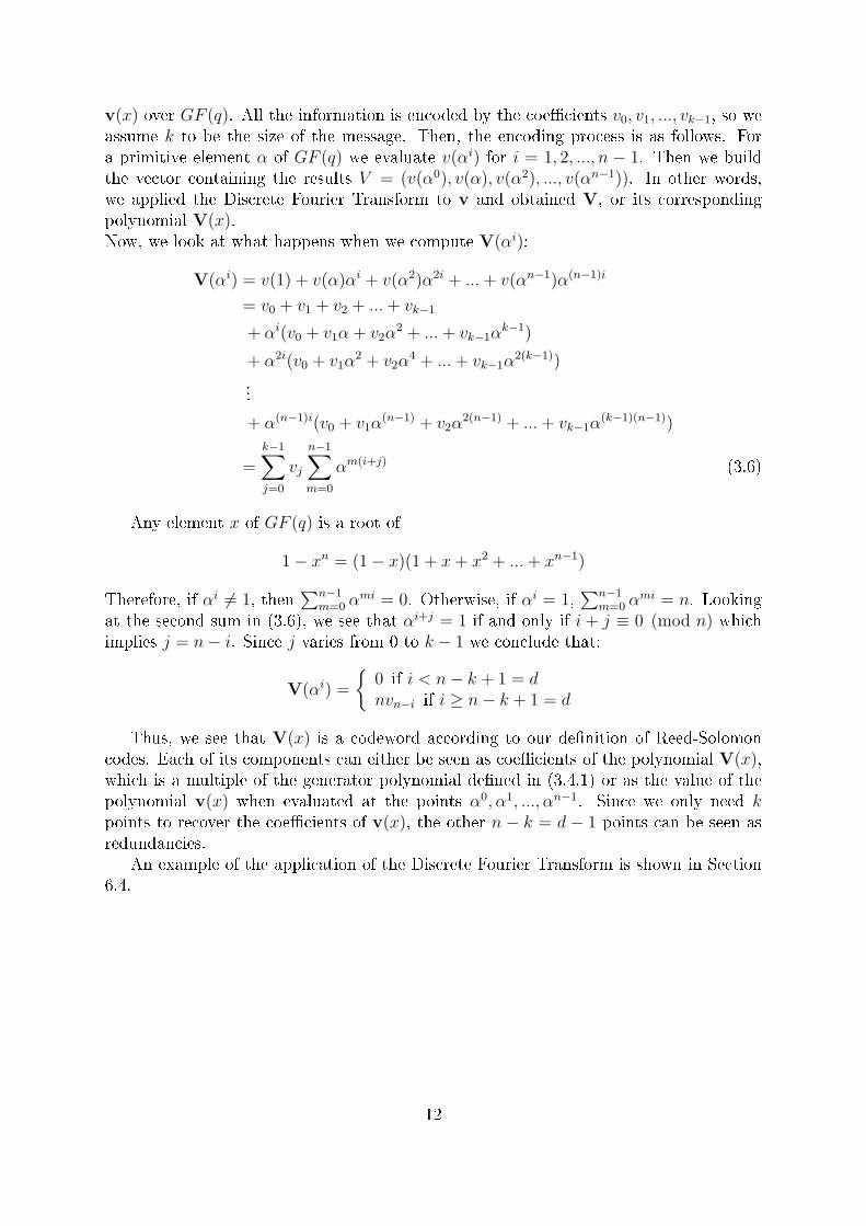
v(x) over GF (q). All the information is encoded by the coe�cients v0, v1, ..., vk−1, so weassume k to be the size of the message. Then, the encoding process is as follows. Fora primitive element α of GF (q) we evaluate v(αi) for i = 1, 2, ..., n − 1. Then we buildthe vector containing the results V = (v(α0), v(α), v(α2), ..., v(αn−1)). In other words,we applied the Discrete Fourier Transform to v and obtained V, or its correspondingpolynomial V(x).Now, we look at what happens when we compute V(αi):
V(αi) = v(1) + v(α)αi + v(α2)α2i + ...+ v(αn−1)α(n−1)i
= v0 + v1 + v2 + ...+ vk−1
+ αi(v0 + v1α + v2α2 + ...+ vk−1α
k−1)
+ α2i(v0 + v1α2 + v2α
4 + ...+ vk−1α2(k−1))
...
+ α(n−1)i(v0 + v1α(n−1) + v2α
2(n−1) + ...+ vk−1α(k−1)(n−1))
=k−1∑j=0
vj
n−1∑m=0
αm(i+j) (3.6)
Any element x of GF (q) is a root of
1− xn = (1− x)(1 + x+ x2 + ...+ xn−1)
Therefore, if αi 6= 1, then∑n−1
m=0 αmi = 0. Otherwise, if αi = 1,
∑n−1m=0 α
mi = n. Lookingat the second sum in (3.6), we see that αi+j = 1 if and only if i + j ≡ 0 (mod n) whichimplies j = n− i. Since j varies from 0 to k − 1 we conclude that:
V(αi) =
{0 if i < n− k + 1 = dnvn−i if i ≥ n− k + 1 = d
Thus, we see that V(x) is a codeword according to our de�nition of Reed-Solomoncodes. Each of its components can either be seen as coe�cients of the polynomial V(x),which is a multiple of the generator polynomial de�ned in (3.4.1) or as the value of thepolynomial v(x) when evaluated at the points α0, α1, ..., αn−1. Since we only need kpoints to recover the coe�cients of v(x), the other n − k = d − 1 points can be seen asredundancies.
An example of the application of the Discrete Fourier Transform is shown in Section6.4.
12
Chapter 4
Fuzzy Extractors and PUFs
Physically Unclonable Functions provide a tamper-resilient method to assign a crypto-graphic key to a hardware device. However, the same dependency upon physical param-eters that give PUFs their protection against active attacks causes their responses to benaturally noisy. The basic premise of PUFs is, nonetheless, that the �distance� betweentwo responses from the same PUF is much smaller than the distance between responsesfrom di�erent PUFs, so that even in the presence of noise it is possible to distinguishresponses originating from di�erent PUF devices.
However, cryptography in general relies on the existence of precisely reproduciblekeys. This means that in order for us to take full advantage of the physical unclonabilityof PUFs we must �nd tools that allow us to cope with this noise. Moreover, it is expectedthat the distribution of PUF responses across multiple PUF devices will not be uniform,and this poses a second problem to the use of PUFs in cryptographic applications. Inorder to address these two issues, namely the small variations in the responses of the samePUF and the nonuniform distribution of responses among di�erent PUFs, the concept ofa fuzzy extractor, initially introduced in [4], is brought into play.
4.1 Basic Ideas
A fuzzy extractor is a primitive that allows the extraction of uniformly random stringsfrom a nonuniform source in a noise-tolerant way. Since there are basically two separateissues being addressed here, it is natural to think that fuzzy extractors will consist oftwo independent steps. This turns out to be the case: �rst we have the informationreconciliation phase, in which a noisy version of the output of a PUF is converted into anoise-free one. A privacy ampli�cation phase follows, extracting randomness out of thenoiseless version of the PUF output.
Regarding the information reconciliation phase, one might ask what we mean bya noiseless version of the PUF response, since all possible outputs seem noisy whencompared to others. The idea here is that prior to the deployment of the device, extensivetesting can be performed in order to determine the expected outcome or, even in theabsence of a prevalent response, we can arbitrarily pick one of the responses as in theneighborhood of the most likely responses as �the noise-free version�. This follows our�rst mathematical model for a PUF, given in Section 2.1.1.
A second question that one might ask, especially when an expected outcome cannot be
13
easily determined from multiple responses, is how a fuzzy extractor can remove the noisefrom a particular PUF response if it has nothing to compare it against. In other words,how can outside information about the noiseless response of the PUF be introduced intothe system? This is done by means of a Helper String.
When a PUF device equipped with a fuzzy extractor system receives a helper stringfrom whoever is trying to verify the identity of the device, it obtains just enough informa-tion to eliminate its response variations and output a consistent response. However, thehelper data is assumed to be public, and therefore must not reveal any useful informationabout the PUF response to someone other than the PUF device itself. In some sense, thehelper data can be thought of as a hint that only makes sense to the person to which itis given.
Once a �clean� response is obtained, traditional techniques for randomness extraction,such as hash functions, can be employed. This allows us to obtain PUF responses thatare almost uniformly distributed across di�erent PUF devices.
In the next sections, we give precise mathematical de�nitions and examples of theprimitives mentioned here.
4.2 Preliminary De�nitions
Before we describe the concepts of secure sketches and fuzzy extractors, we must �rstintroduce a few basic de�nitions, by following [4]. In general,M will denote the metricspace being considered, with a distance function dis :M×M→ R+. We will mostly bedealing with Hamming distances on the setsM = Fn.
In order to study the security of secure sketches and fuzzy extractors, we must �rstbe able to quantify how secure a given random variable is. For this purpose, we use themin-entropy:
De�nition 4.1. Min-Entropy: The min-entropy of a random variable A measures itsunpredictability, or how hard it is for someone to guess its output. It is given by:
H∞(A)def= − log
(maxaP (A = a)
)(4.1)
For our purposes however, we will be more interested in the cases where we want toconsider how hard it is for an adversary to guess the value of a random variable A, ifhe/she �nds out the value of another random variable B.
De�nition 4.2. Average Min-Entropy: The average min-entropy measures the unpre-dictability of a random variable A, given the value of another random variable B. It isde�ned as:
H̃∞(A |B)def= − log
(Eb←B
[maxaP (A = a |B = b)
])(4.2)
Because we are looking for secure sketches and fuzzy extractor's outputs that lookuniformly random to an observer, we need a way to measure how close to uniform arandom variable is. This is accomplished with the concept of statistical distance:
14
De�nition 4.3. Statistical Distance: The statistical distance measures how statisticallyapart are two discrete random variables. It is given by:
SD(A,B) =1
2
∑x
|P (A = v)− P (B = v)| (4.3)
In all these expressions, and throughout this report, P (A = a) will refer to theprobability that A = a and log x will refer to the logarithm base 2 of x.
4.3 Secure Sketches
LetM be a metric space with distance function dis .
De�nition 4.4. [4] An (M,m, m̃, t)-secure sketch is a pair of randomized procedures,�sketch� (SS ) and �recover� (Rec ), with the following properties:
1. The sketching procedure SS on input w ∈M returns a bit string s ∈ {0, 1}∗.
2. The recovery procedure Rec takes an element w′ ∈M and a bit string s ∈ {0, 1}∗.The correctness property of secure sketches guarantees that if dis (w,w′) ≤ t, thenRec (w′, SS (w)) = w. If dis (w,w′) > t, no guarantee is provided about the outputof Rec .
3. The security property guarantees that for any distribution W over M with min-entropy m, the value of W can be recovered by the adversary who observes s withprobability no greater than 2−m̃. That is, H̃∞(W | SS (W )) ≥ m̃.
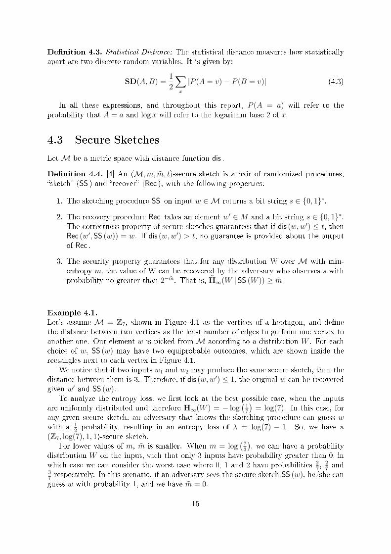
Example 4.1.Let's assume M = Z7, shown in Figure 4.1 as the vertices of a heptagon, and de�nethe distance between two vertices as the least number of edges to go from one vertex toanother one. Our element w is picked fromM according to a distribution W . For eachchoice of w, SS (w) may have two equiprobable outcomes, which are shown inside therectangles next to each vertex in Figure 4.1.
We notice that if two inputs w1 and w2 may produce the same secure sketch, then thedistance between them is 3. Therefore, if dis (w,w′) ≤ 1, the original w can be recoveredgiven w′ and SS (w).
To analyze the entropy loss, we �rst look at the best possible case, when the inputsare uniformly distributed and therefore H∞(W ) = − log
(17
)= log(7). In this case, for
any given secure sketch, an adversary that knows the sketching procedure can guess wwith a 1
2probability, resulting in an entropy loss of λ = log(7) − 1. So, we have a
(Z7, log(7), 1, 1)-secure sketch.For lower values of m, m̃ is smaller. When m = log
(73
), we can have a probability
distribution W on the input, such that only 3 inputs have probability greater than 0, inwhich case we can consider the worst case where 0, 1 and 2 have probabilities 2
7, 2
7and
37respectively. In this scenario, if an adversary sees the secure sketch SS (w), he/she can
guess w with probability 1, and we have m̃ = 0.
15
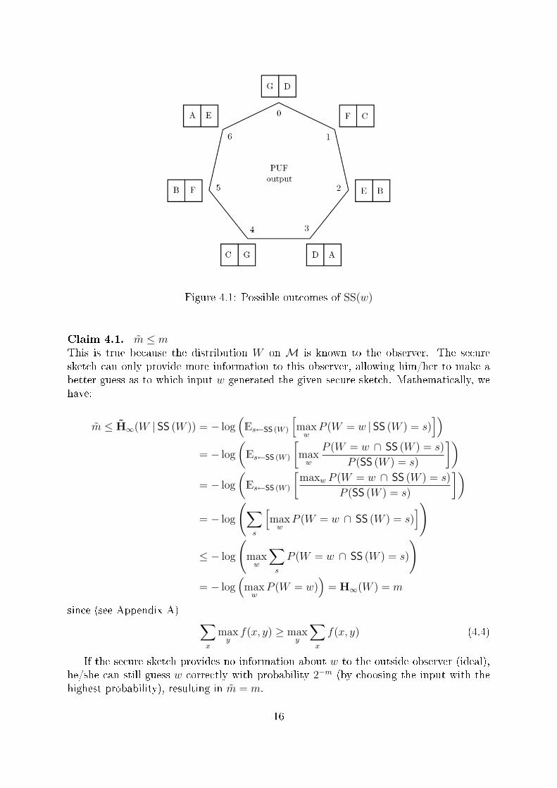
Figure 4.1: Possible outcomes of SS(w)
Claim 4.1. m̃ ≤ mThis is true because the distribution W on M is known to the observer. The securesketch can only provide more information to this observer, allowing him/her to make abetter guess as to which input w generated the given secure sketch. Mathematically, wehave:
m̃ ≤ H̃∞(W | SS (W )) = − log(Es←SS (W )
[maxw
P (W = w | SS (W ) = s)])
= − log
(Es←SS (W )
[maxw
P (W = w ∩ SS (W ) = s)
P (SS (W ) = s)
])= − log
(Es←SS (W )
[maxw P (W = w ∩ SS (W ) = s)
P (SS (W ) = s)
])= − log
(∑s
[maxw
P (W = w ∩ SS (W ) = s)])
≤ − log
(maxw
∑s
P (W = w ∩ SS (W ) = s)
)= − log
(maxw
P (W = w))
= H∞(W ) = m
since (see Appendix A) ∑x
maxyf(x, y) ≥ max
y
∑x
f(x, y) (4.4)
If the secure sketch provides no information about w to the outside observer (ideal),he/she can still guess w correctly with probability 2−m (by choosing the input with thehighest probability), resulting in m̃ = m.
16
4.4 The Code-O�set construction
For practical applications, a good secure sketch construction must have e�cient Rec andSS procedures and must minimize the entropy loss λ = m− m̃. Example 4.1 illustratesa case in which the entropy loss is very signi�cant. That same example also suggests theexistence of an underlying code, since we are essentially correcting errors whenever theyare not too numerous. In the same sense, trying to �nd a good secure sketch is a similarproblem to looking for a good code, since we try to maximize the distance betweeninputs with the same secure sketch while trying to have as many secure sketches aspossible. This connection between secure sketches and codes becomes even clearer whenwe consider a Code-O�set construction, which provides an e�cient and very practicalmethod for designing secure sketches. It is de�ned as follows (see [4]).
We assume the existence of an [n, k, d] code C with codewords de�ned on the samespace M = Fn from which the inputs are taken. We also de�ne the distance to be theHamming distance. For a given input w, the sketching procedure produces SS (w) =w+C(x), where x is a random element from Fk, so that c = C(x) is a random codeword.For the recovery procedure Rec , we assume an input w′ such that dis (w,w′) ≤ bd−1
2c, and
we start by subtracting it from its secure sketch to obtain c′ = w+ c−w′ = c+ (w−w′).Since the Hamming weight of w − w′ is less than bd−1
2c, we know that dis (c, c′) ≤ bd−1
2c
and we can apply a decoding algorithm to obtain the codeword c. Once we have c, wecan simply subtract it from the secure sketch to obtain (w + c) − c = w. So we outputRec (w′, SS (w)) = w.
This construction also presents the advantage that the secure sketch is just anotherelement of Fn and therefore does not represent a problem in terms of storage, as opposedto a secure sketch construction using fuzzy vaults (see [9]) for example. In the remainderof this section, we will mostly deal with secure sketches based on linear codes de�nedover binary �elds, in which addition and subtraction are equivalent, slightly simplifyingthe operations described above.
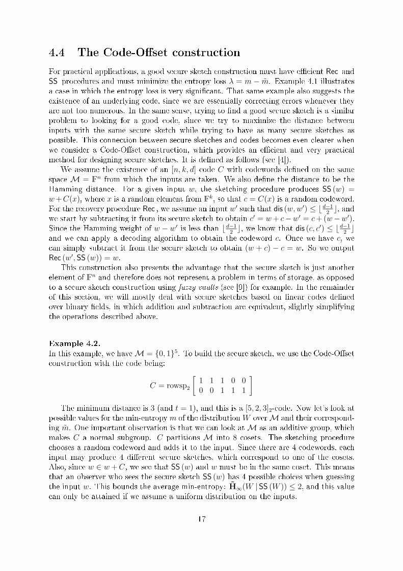
Example 4.2.In this example, we haveM = {0, 1}5. To build the secure sketch, we use the Code-O�setconstruction with the code being:
C = rowsp2
[1 1 1 0 00 0 1 1 1
]The minimum distance is 3 (and t = 1), and this is a [5, 2, 3]2-code. Now let's look at
possible values for the min-entropym of the distributionW overM and their correspond-ing m̃. One important observation is that we can look atM as an additive group, whichmakes C a normal subgroup. C partitions M into 8 cosets. The sketching procedurechooses a random codeword and adds it to the input. Since there are 4 codewords, eachinput may produce 4 di�erent secure sketches, which correspond to one of the cosets.Also, since w ∈ w+C, we see that SS (w) and w must be in the same coset. This meansthat an observer who sees the secure sketch SS (w) has 4 possible choices when guessingthe input w. This bounds the average min-entropy: H̃∞(W | SS (W )) ≤ 2, and this valuecan only be attained if we assume a uniform distribution on the inputs.
17
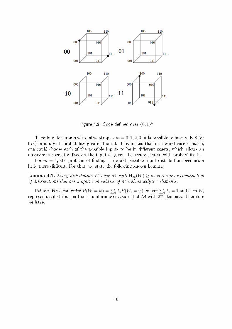
Figure 4.2: Code de�ned over {0, 1}5
Therefore, for inputs with min-entropies m = 0, 1, 2, 3, it is possible to have only 8 (orless) inputs with probability greater than 0. This means that in a worst-case scenario,one could choose each of the possible inputs to be in di�erent cosets, which allows anobserver to correctly discover the input w, given the secure sketch, with probability 1.
For m = 4, the problem of �nding the worst possible input distribution becomes alittle more di�cult. For that, we state the following known Lemma:
Lemma 4.1. Every distribution W overM with H∞(W ) ≥ m is a convex combinationof distributions that are uniform on subsets of M with exactly 2m elements.
Using this we can write P (W = w) =∑
i λiP (Wi = w), where∑
i λi = 1 and each Wi
represents a distribution that is uniform over a subset ofM with 2m elements. Thereforewe have:
18
H̃∞(W | SS (W )) = − log(Es←SS (W )
[maxw
P (W = w | SS (W ) = s)])
= − log
(Es←SS (W )
[maxw
∑i
λiP (Wi = w | SS (W ) = s)
])
≥ − log
(Es←SS (W )
[∑i
λi maxw
P (Wi = w | SS (W ) = s)
])
= − log
(∑i
λiEs←SS (W )
[maxw
P (Wi = w | SS (W ) = s)])
≥ − log(
maxiEs←SS (W )
[maxw
P (Wi = w | SS (W ) = s)])
= − log(Es←SS (W )
[maxw
P (Wk = w | SS (W ) = s)])
= H̃∞(Wk | SS (W )) (4.5)
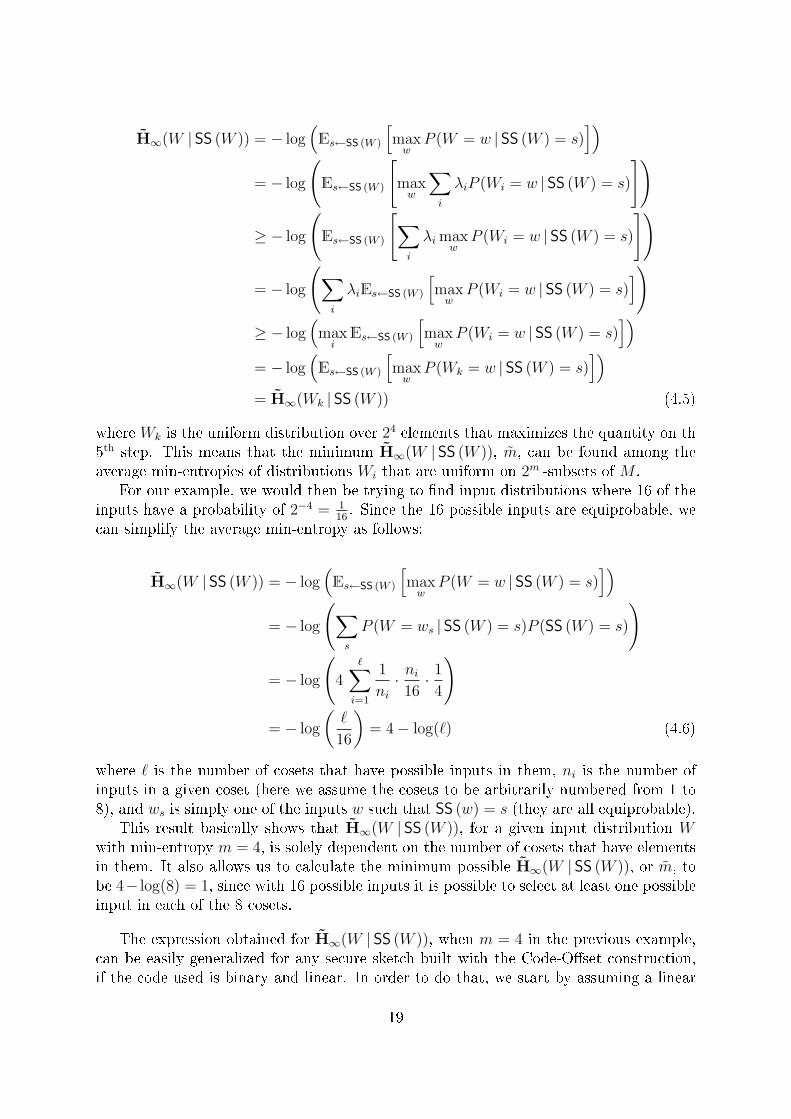
where Wk is the uniform distribution over 24 elements that maximizes the quantity on th5th step. This means that the minimum H̃∞(W | SS (W )), m̃, can be found among theaverage min-entropies of distributions Wi that are uniform on 2m -subsets of M .
For our example, we would then be trying to �nd input distributions where 16 of theinputs have a probability of 2−4 = 1
16. Since the 16 possible inputs are equiprobable, we
can simplify the average min-entropy as follows:
H̃∞(W | SS (W )) = − log(Es←SS (W )
[maxw
P (W = w | SS (W ) = s)])
= − log
(∑s
P (W = ws | SS (W ) = s)P (SS (W ) = s)
)
= − log
(4∑̀i=1
1
ni· ni
16· 1
4
)
= − log
(`
16
)= 4− log(`) (4.6)
where ` is the number of cosets that have possible inputs in them, ni is the number ofinputs in a given coset (here we assume the cosets to be arbitrarily numbered from 1 to8), and ws is simply one of the inputs w such that SS (w) = s (they are all equiprobable).
This result basically shows that H̃∞(W | SS (W )), for a given input distribution Wwith min-entropy m = 4, is solely dependent on the number of cosets that have elementsin them. It also allows us to calculate the minimum possible H̃∞(W | SS (W )), or m̃, tobe 4− log(8) = 1, since with 16 possible inputs it is possible to select at least one possibleinput in each of the 8 cosets.
The expression obtained for H̃∞(W | SS (W )), when m = 4 in the previous example,can be easily generalized for any secure sketch built with the Code-O�set construction,if the code used is binary and linear. In order to do that, we start by assuming a linear
19
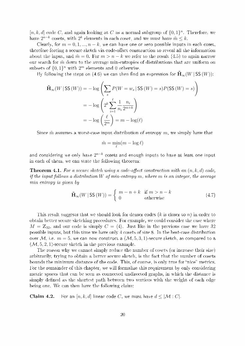
[n, k, d] code C, and again looking at C as a normal subgroup of {0, 1}n. Therefore, wehave 2n−k cosets, with 2k elements in each coset, and we must have m̃ ≤ k.
Clearly, for m = 0, 1, ..., n− k, we can have one or zero possible inputs in each coset,therefore forcing a secure sketch via code-o�set construction to reveal all the informationabout the input, and m̃ = 0. For m > n− k we refer to the result (4.5) to again narrowour search for m̃ down to the average min-entropies of distributions that are uniform onsubsets of {0, 1}n with 2m elements and 0 otherwise.
By following the steps on (4.6) we can then �nd an expression for H̃∞(W | SS (W )):
H̃∞(W | SS (W )) = − log
(∑s
P (W = ws | SS (W ) = s)P (SS (W ) = s)
)
= − log
(2k∑̀i=1
1
ni
ni2m+k
)
= − log
(`
2m
)= m− log(`)
Since m̃ assumes a worst-case input distribution of entropy m, we simply have that
m̃ = min`
(m− log `)
and considering we only have 2n−k cosets and enough inputs to have at least one inputin each of them, we can state the following theorem:
Theorem 4.1. For a secure sketch using a code-o�set construction with an (n, k, d) code,if the input follows a distribution W of min-entropy m, where m is an integer, the averagemin-entropy is given by
H̃∞(W | SS (W )) =
{m− n+ k if m > n− k0 otherwise
(4.7)
This result suggests that we should look for denser codes (k is closer to n) in order toobtain better secure sketching procedures. For example, we could consider the case whereM = Z32, and our code is simply C = 〈4〉. Just like in the previous case we have 32possible inputs, but this time we have only 4 cosets of size 8. In the best-case distributionoverM, i.e. m = 5, we can now construct a (M, 5, 3, 1)-secure sketch, as compared to a(M, 5, 2, 1)-secure sketch in the previous example.
The reason why we cannot simply reduce the number of cosets (or increase their size)arbitrarily, trying to obtain a better secure sketch, is the fact that the number of cosetsbounds the minimum distance of the code. This, of course, is only true for �nice� metrics.For the remainder of this chapter, we will formalize this requirement by only consideringmetric spaces that can be seen as connected undirected graphs, in which the distance issimply de�ned as the shortest path between two vertices with the weight of each edgebeing one. We can then have the following claim:
Claim 4.2. For an [n, k, d] linear code C, we must have d ≤ |M : C|.
20
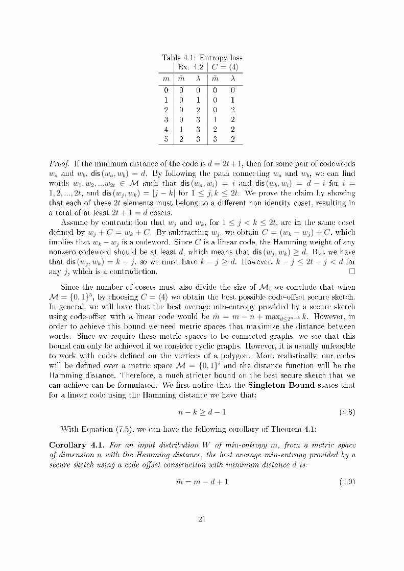
Table 4.1: Entropy lossEx. 4.2 C = 〈4〉
m m̃ λ m̃ λ
0 0 0 0 01 0 1 0 12 0 2 0 23 0 3 1 24 1 3 2 25 2 3 3 2
Proof. If the minimum distance of the code is d = 2t+1, then for some pair of codewordswa and wb, dis (wa, wb) = d. By following the path connecting wa and wb, we can �ndwords w1, w2, ...w2t ∈ M such that dis (wa, wi) = i and dis (wb, wi) = d − i for i =1, 2, ..., 2t, and dis (wj, wk) = |j − k| for 1 ≤ j, k ≤ 2t. We prove the claim by showingthat each of these 2t elements must belong to a di�erent non-identity coset, resulting ina total of at least 2t+ 1 = d cosets.
Assume by contradiction that wj and wk, for 1 ≤ j < k ≤ 2t, are in the same cosetde�ned by wj + C = wk + C. By subtracting wj, we obtain C = (wk − wj) + C, whichimplies that wk−wj is a codeword. Since C is a linear code, the Hamming weight of anynonzero codeword should be at least d, which means that dis (wj, wk) ≥ d. But we havethat dis (wj, wk) = k − j, so we must have k − j ≥ d. However, k − j ≤ 2t − j < d forany j, which is a contradiction.
Since the number of cosets must also divide the size of M, we conclude that whenM = {0, 1}5, by choosing C = 〈4〉 we obtain the best possible code-o�set secure sketch.In general, we will have that the best average min-entropy provided by a secure sketchusing code-o�set with a linear code would be m̃ = m − n + maxd≤2n−k k. However, inorder to achieve this bound we need metric spaces that maximize the distance betweenwords. Since we require these metric spaces to be connected graphs, we see that thisbound can only be achieved if we consider cyclic graphs. However, it is usually unfeasibleto work with codes de�ned on the vertices of a polygon. More realistically, our codeswill be de�ned over a metric space M = {0, 1}i and the distance function will be theHamming distance. Therefore, a much stricter bound on the best secure sketch that wecan achieve can be formulated. We �rst notice that the Singleton Bound states thatfor a linear code using the Hamming distance we have that:
n− k ≥ d− 1 (4.8)
With Equation (7.5), we can have the following corollary of Theorem 4.1:
Corollary 4.1. For an input distribution W of min-entropy m, from a metric spaceof dimension n with the Hamming distance, the best average min-entropy provided by asecure sketch using a code-o�set construction with minimum distance d is:
m̃ = m− d+ 1 (4.9)
21
This result con�rms our intuition that there is a trade-o� between the error-correctingcapability of a Rec procedure of a secure sketch and how much information leaks by thepublishing of the secure sketch. By noticing that for a code to achieve the Singletonbound, we must have d = 2t + 1, where t is the error-correcting bound of the code, we�nd that
m̃ = m− 2t
which means that to increase the noise-tolerance by one bit, we must in fact lose twobits of entropy. This creates an inherent limitation to the noise-tolerance levels of securesketches and also to fuzzy extractors (see next section) built on top of secure sketches,especially in a setting where a large amount of noise is expected at the output of a PUF.
4.5 Fuzzy Extractors
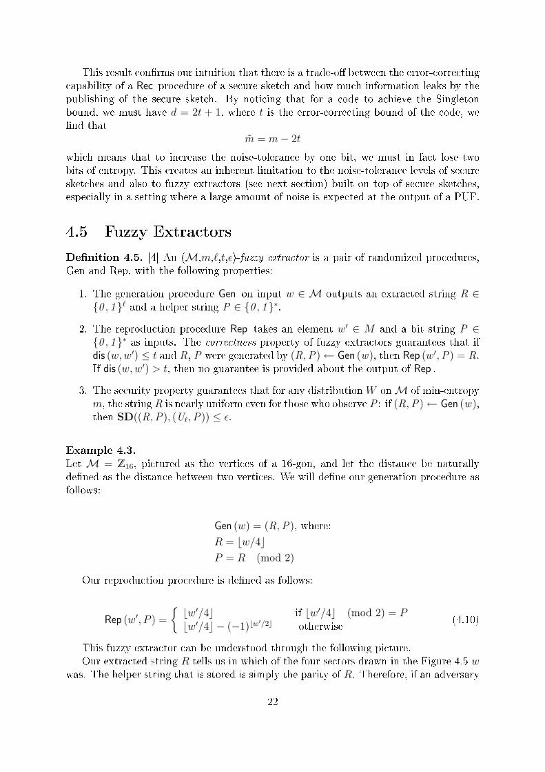
De�nition 4.5. [4] An (M,m,`,t,ε)-fuzzy extractor is a pair of randomized procedures,Gen and Rep, with the following properties:
1. The generation procedure Gen on input w ∈ M outputs an extracted string R ∈{0 , 1}` and a helper string P ∈ {0 , 1}∗.
2. The reproduction procedure Rep takes an element w′ ∈ M and a bit string P ∈{0 , 1}∗ as inputs. The correctness property of fuzzy extractors guarantees that ifdis (w,w′) ≤ t and R, P were generated by (R,P)← Gen (w), then Rep (w′,P) = R.If dis (w,w′) > t, then no guarantee is provided about the output of Rep .
3. The security property guarantees that for any distributionW onM of min-entropym, the string R is nearly uniform even for those who observe P : if (R,P)← Gen (w),then SD((R,P), (U`,P)) ≤ ε.
Example 4.3.Let M = Z16, pictured as the vertices of a 16-gon, and let the distance be naturallyde�ned as the distance between two vertices. We will de�ne our generation procedure asfollows:
Gen (w) = (R,P), where:
R = bw/4cP = R (mod 2)
Our reproduction procedure is de�ned as follows:
Rep (w′, P ) =
{bw′/4c if bw′/4c (mod 2) = Pbw′/4c − (−1)bw
′/2c otherwise(4.10)
This fuzzy extractor can be understood through the following picture.Our extracted string R tells us in which of the four sectors drawn in the Figure 4.5 w
was. The helper string that is stored is simply the parity of R. Therefore, if an adversary
22
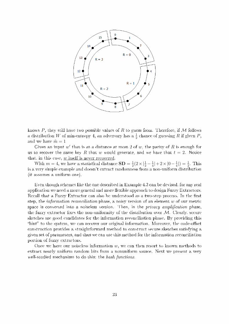
knows P , they still have two possible values of R to guess from. Therefore, ifM followsa distribution W of min-entropy 4, an adversary has a 1
2chance of guessing R if given P ,
and we have m̃ = 1Given an input w′ that is at a distance at most 2 of w, the parity of R is enough for
us to recover the same key R that w would generate, and we have that t = 2. Noticethat, in this case, w itself is never recovered.
With m = 4, we have a statistical distance SD = 12(2×|1
2− 1
4|+2×|0− 1
4|) = 1
2. This
is a very simple example and doesn't extract randomness from a non-uniform distribution(it assumes a uniform one).
Even though schemes like the one described in Example 4.3 can be devised, for any realapplication we need a more general and more �exible approach to design Fuzzy Extractors.Recall that a Fuzzy Extractor can also be understood as a two-step process. In the �rststep, the information reconciliation phase, a noisy version of an element w of our metricspace is converted into a noiseless version. Then, in the privacy ampli�cation phase,the fuzzy extractor �xes the non-uniformity of the distribution overM. Clearly, securesketches are good candidates for the information reconciliation phase. By providing this�hint� to the system, we can recover our original information. Moreover, the code-o�setconstruction provides a straightforward method to construct secure sketches satisfying agiven set of parameters, and thus we can use this method for the information reconciliationportion of fuzzy extractors.
Once we have our noiseless information w, we can then resort to known methods toextract nearly uniform random bits from a nonuniform source. Next we present a verywell-studied mechanism to do this: the hash functions.
23
4.6 Hash Functions
A hash function is used when we have a non-uniform distribution on some source and wewish to extract a uniform distribution with roughly the same entropy. For example, ifwe have a space of binary 10-tuples with all elements having the �rst four digits being 0,we in fact only have six bits of information. A hash function in essence reduces the sizeof our space to re�ect the actual amount of information in it.
Formally, a hash function is a mapping from {0, 1}i, the keys, to {0, 1}j, the values.Following [20], there are three properties of a cryptographic hash function:
1. A hash function h is a one way hash function if, for a random x ∈ {0, 1}i, givenh(x), it is hard to compute y ∈ {0, 1}i such that h(y) = h(x).
2. The hash of a key should be computed in polynomial time, and is sometimes per-formed in linear time in the length of the input.
3. A hash function is called strongly collision free if it is computationally infeasible to�nd two keys x1, x2 such that h(x1) = h(x2). A hash function is weakly collisionfree if, given a key x, it is computationally infeasible to �nd an x′ 6= x such thath(x) = h(x′).
A hash family consists of a set K of keys, a set V of values, and a set H of hashfunctions which map keys to values.
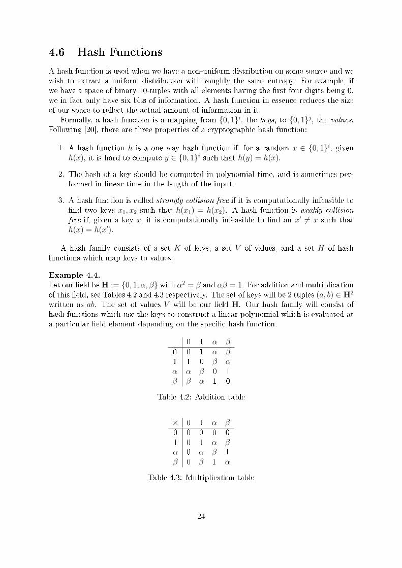
Example 4.4.Let our �eld beH := {0, 1, α, β} with α2 = β and αβ = 1. For addition and multiplicationof this �eld, see Tables 4.2 and 4.3 respectively. The set of keys will be 2 tuples (a, b) ∈ H2
written as ab. The set of values V will be our �eld H. Our hash family will consist ofhash functions which use the keys to construct a linear polynomial which is evaluated ata particular �eld element depending on the speci�c hash function.
+ 0 1 α β0 0 1 α β1 1 0 β αα α β 0 1β β α 1 0
Table 4.2: Addition table
× 0 1 α β0 0 0 0 01 0 1 α βα 0 α β 1β 0 β 1 α
Table 4.3: Multiplication table
24
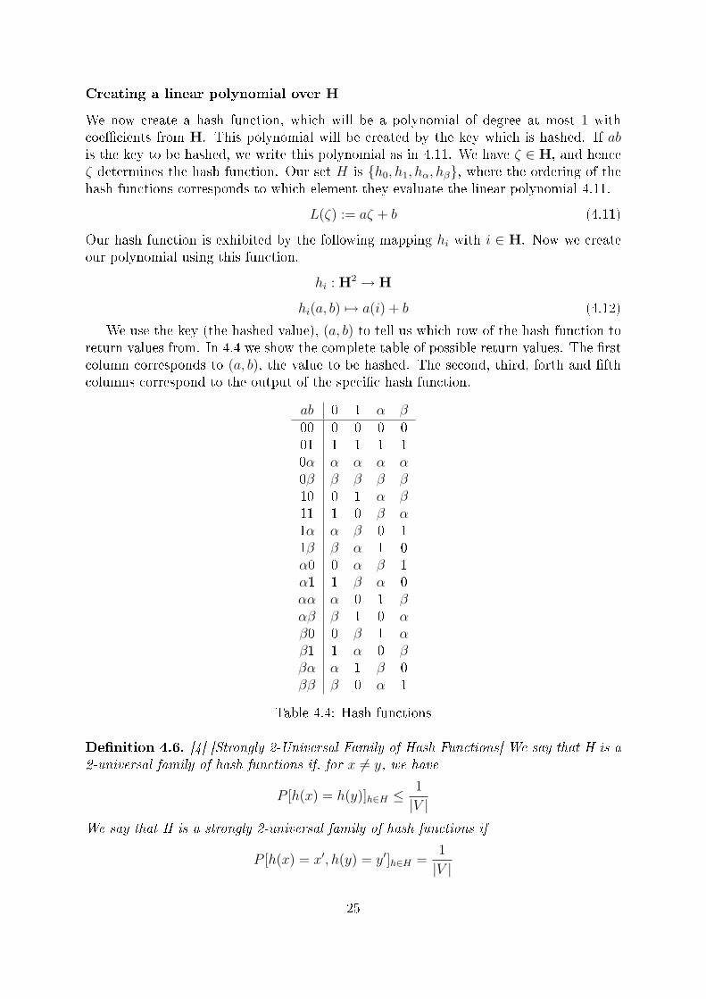
Creating a linear polynomial over H
We now create a hash function, which will be a polynomial of degree at most 1 withcoe�cients from H. This polynomial will be created by the key which is hashed. If abis the key to be hashed, we write this polynomial as in 4.11. We have ζ ∈ H, and henceζ determines the hash function. Our set H is {h0, h1, hα, hβ}, where the ordering of thehash functions corresponds to which element they evaluate the linear polynomial 4.11.
L(ζ) := aζ + b (4.11)
Our hash function is exhibited by the following mapping hi with i ∈ H. Now we createour polynomial using this function.
hi : H2 → H
hi(a, b) 7→ a(i) + b (4.12)
We use the key (the hashed value), (a, b) to tell us which row of the hash function toreturn values from. In 4.4 we show the complete table of possible return values. The �rstcolumn corresponds to (a, b), the value to be hashed. The second, third, forth and �fthcolumns correspond to the output of the speci�c hash function.
ab 0 1 α β00 0 0 0 001 1 1 1 10α α α α α0β β β β β10 0 1 α β11 1 0 β α1α α β 0 11β β α 1 0α0 0 α β 1α1 1 β α 0αα α 0 1 βαβ β 1 0 αβ0 0 β 1 αβ1 1 α 0 ββα α 1 β 0ββ β 0 α 1
Table 4.4: Hash functions
De�nition 4.6. [4] [Strongly 2-Universal Family of Hash Functions] We say that H is a2-universal family of hash functions if, for x 6= y, we have
P [h(x) = h(y)]h∈H ≤1
|V |We say that H is a strongly 2-universal family of hash functions if
P [h(x) = x′, h(y) = y′]h∈H =1
|V |
25
Claim 4.3. Our example is a 2 universal family of hash functions.
Proof. We need to show that P [h(x) = h(y)] ≤ 1|V |
Since h ∈ H is �xed, we only look at one column of 4.4 chosen uniformly at random.Since each column has the same number of occurrences of each value, we will look at justone column. For x ∈ H2 there are exactly 3 other keys which hash to the same value asx. Since there are 15 values that y can take, we conclude
P [h(x) = h(y)]h∈H =3
16≤ 1
4
We conclude that our example is a 2 universal family of hash functions.
4.7 Overall design of fuzzy extractors
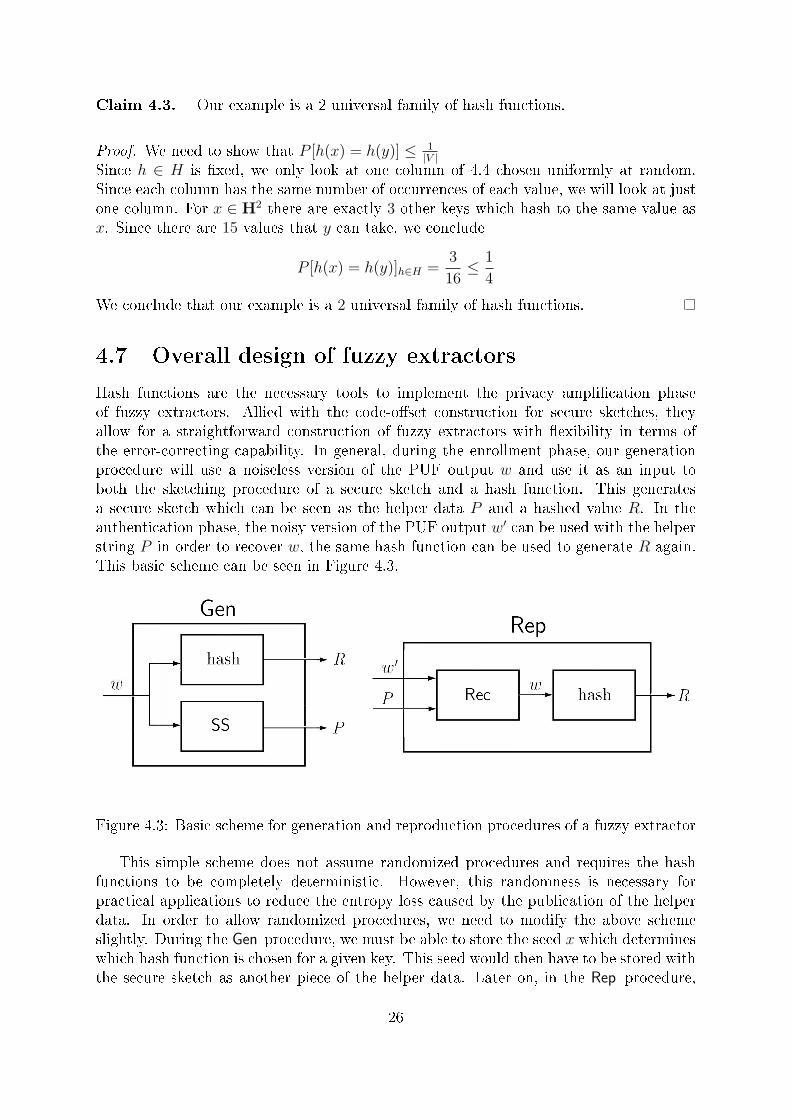
Hash functions are the necessary tools to implement the privacy ampli�cation phaseof fuzzy extractors. Allied with the code-o�set construction for secure sketches, theyallow for a straightforward construction of fuzzy extractors with �exibility in terms ofthe error-correcting capability. In general, during the enrollment phase, our generationprocedure will use a noiseless version of the PUF output w and use it as an input toboth the sketching procedure of a secure sketch and a hash function. This generatesa secure sketch which can be seen as the helper data P and a hashed value R. In theauthentication phase, the noisy version of the PUF output w′ can be used with the helperstring P in order to recover w, the same hash function can be used to generate R again.This basic scheme can be seen in Figure 4.3.
Figure 4.3: Basic scheme for generation and reproduction procedures of a fuzzy extractor
This simple scheme does not assume randomized procedures and requires the hashfunctions to be completely deterministic. However, this randomness is necessary forpractical applications to reduce the entropy loss caused by the publication of the helperdata. In order to allow randomized procedures, we need to modify the above schemeslightly. During the Gen procedure, we must be able to store the seed x which determineswhich hash function is chosen for a given key. This seed would then have to be stored withthe secure sketch as another piece of the helper data. Later on, in the Rep procedure,
26
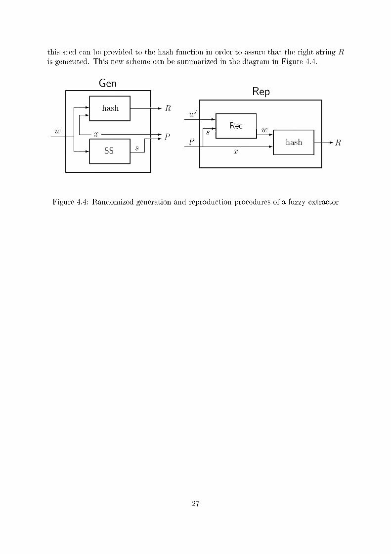
this seed can be provided to the hash function in order to assure that the right string Ris generated. This new scheme can be summarized in the diagram in Figure 4.4.
Figure 4.4: Randomized generation and reproduction procedures of a fuzzy extractor
27
Chapter 5
Hardware implementation of Fuzzy
Extractors
One of the most appealing qualities of a PUF-based authentication system is the fact thatPUFs can � and in fact have to � be implemented in hardware. This provides a securityscheme for lightweight and low-cost hardware devices, such as RFIDs and smartcards [6].However, in order to use fuzzy extractors as a way to obtain reliable cryptographic keysfrom PUFs, while still keeping PUFs attractive for these lightweight hardware devices, afuzzy extractor must be implemented in hardware as well. Moreover, its implementationshould be fairly area-e�cient, or it will defeat the purpose of using PUFs in small hardwaredevices.
The code-o�set/hash-function construction depicted in Figure 4.4 has the advantageof giving �exibility in terms of error-correction and security parameters. The most com-plex component of this scheme is the decoder that must be implemented for the recoveryprocedure of the secure sketch. Therefore, in this section we present a compact imple-mentation for a decoder, which still provides good error-correcting capabilities.
5.1 BCH codes and Fuzzy Extractors
BCH codes are very powerful error-correcting codes. Even though they cannot be imple-mented as easily as other codes, such as Reed-Muller codes, an area-e�cient hardwareimplementation is still feasible. This makes them very good candidates for being usedin the context of fuzzy extractors. Linear codes are very important pieces in Fuzzy Ex-tractors, in particular for the information reconciliation phase. We perform this task byusing a secure sketch with a code-o�set construction. Therefore, we need to be able togenerate a random codeword, i.e. encode a random message, for the sketching procedureand to do decoding for the recovery procedure.
During the enrollment phase the device can be characterized more accurately by takingmultiple samples and averaging to minimize noise. This is followed by the application ofthe sketching procedure which can be performed o�ine via software. Since this occursprior to the deployment of the device and does not need to be done by the device itself,a hardware implementation is only needed for the recovery procedure. Therefore, we willmainly focus on the hardware implementation of a BCH decoder.
28
Since most PUFs output binary responses, and since there is no reason to be concernedabout burst errors, binary codes satisfy our needs and we will be dealing with binary BCHcodes only.
5.2 Hardware architecture for a BCH decoder
For security applications, and more speci�cally for hardware authentication, speed is nota major concern. In other words, it is not fundamental that a device can be correctlyauthenticated in microseconds. However, when we consider applications such as FPGAintellectual property (IP) protection (see [3]), it becomes clear that our main goal is areae�ciency. After all, the authentication circuitry is typically part of a much larger andcomplex circuit, whose IP we want to protect. Therefore, our design focuses on serializingoperations as much as possible, in order to reduce the overall gate count.
5.2.1 Basic steps in BCH decoding
The task of decoding an (n, k, d) BCH code in the communications setting can be sum-marized as follows: given a received polynomial r(x) = v(x) + e(x), we want to �nd theoriginal transmitted polynomial v(x). Equivalently, we can also �nd the error polynomiale(x). While designing the decoder for a binary BCH code, there are mainly four steps wehave to consider.
1. Syndrome computation:We start by computing the 2t syndromes of the received message r(x). That isdone by simply plugging in the 2t roots of the generator polynomial, namely αi fori = 1, 2, ..., 2t, to r(x). Since v(αi) = 0 for i = 1, 2, ..., 2t if v(x) is a codeword, thisis equivalent to computing the syndromes of the error polynomial e(x).
2. Finding the Error-Locator polynomial σ(x):The Error-Locator polynomial σ(x) = 1 + σ1x+ ...+ στx
τ , has τ roots of the formα−ij for j = 1, 2, ..., τ . If α−ik is a root of σ(x) for some k, then the error polynomialhas a coe�cient of 1 in front of its ik
th term. In other words, there was a bit errorat the ik
th position.There are a few di�erent known algorithms for computing the Error-Locator poly-nomial, given the 2t syndromes, such as the Peterson algorithm and the Berlekamp-Massey algorithm.
3. Finding the roots of the Error-Locator polynomial:In the binary case, �nding the roots of σ(x) is enough for us to determine the errorpolynomial e(x), since the only possible coe�cients are 0 (no error at that location)and 1 (error at that location).
4. Finding the transmitted polynomial v(x):In the binary case, this simply means adding the error polynomial to the receivedpolynomial in order to obtain v(x).
29
5.2.2 Syndrome Computation
Syndrome computation in the case of BCH codes basically consists in plugging each ofthe 2t roots of the generator polynomial into the received polynomial. Since these rootsare found in an extension �eld GF (2m), the calculated syndromes are also elements fromGF (2m), and can, therefore, be represented by m bits.The basic approach to computing these syndromes consists in noticing the fact that wecan rewrite the expression for r(αi) (the ith syndrome) as follows
r(αi) = r0 + r1αi + r2α
2i + ...+ rn−1α(n−1)i =
(...(((rn−1αi) + rn−2)α
i) + rn−3)...+ r1)αi + r0 . (5.1)
Equation (5.1) tells us that we can compute the ith syndrome by taking each ofthe binary coe�cients of r(x) starting with the one with the highest degree, adding itto the previous result and then multiplying the result by αi. This recursive recursivecomputation can be e�ciently realized using a Linear Feedback Shift Register (LFSR).
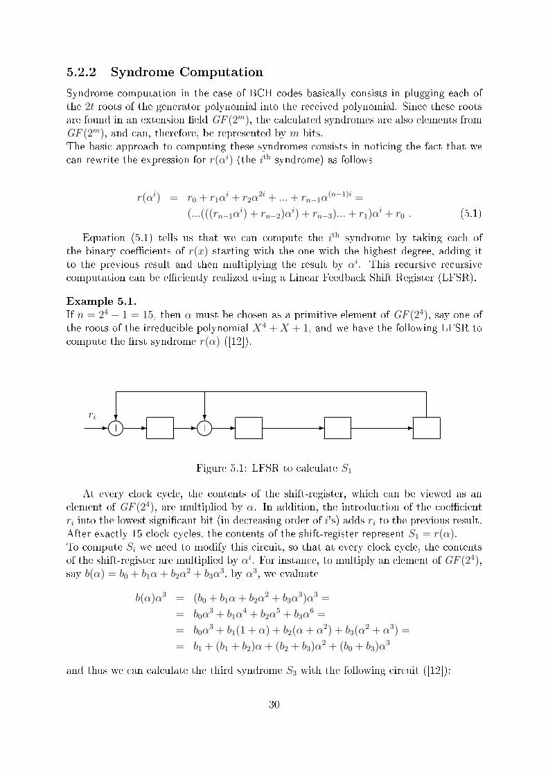
Example 5.1.If n = 24 − 1 = 15, then α must be chosen as a primitive element of GF (24), say one ofthe roots of the irreducible polynomial X4 +X + 1, and we have the following LFSR tocompute the �rst syndrome r(α) ([12]).
- - - -� �� � ��- -+ +
? ?ri
Figure 5.1: LFSR to calculate S1
At every clock cycle, the contents of the shift-register, which can be viewed as anelement of GF (24), are multiplied by α. In addition, the introduction of the coe�cientri into the lowest signi�cant bit (in decreasing order of i's) adds ri to the previous result.After exactly 15 clock cycles, the contents of the shift-register represent S1 = r(α).To compute Si we need to modify this circuit, so that at every clock cycle, the contentsof the shift-register are multiplied by αi. For instance, to multiply an element of GF (24),say b(α) = b0 + b1α + b2α
2 + b3α3, by α3, we evaluate
b(α)α3 = (b0 + b1α + b2α2 + b3α
3)α3 =
= b0α3 + b1α
4 + b2α5 + b3α
6 =
= b0α3 + b1(1 + α) + b2(α + α2) + b3(α
2 + α3) =
= b1 + (b1 + b2)α + (b2 + b3)α2 + (b0 + b3)α
3
and thus we can calculate the third syndrome S3 with the following circuit ([12]):
30
-� �� � �� � �� � ��- - - -+ + + +
? ?
6 6
? ?
6
ri
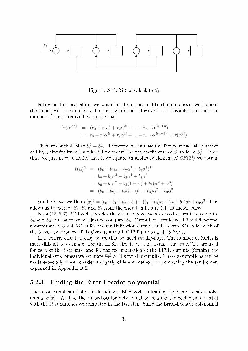
Figure 5.2: LFSR to calculate S3
Following this procedure, we would need one circuit like the one above, with aboutthe same level of complexity, for each syndrome. However, it is possible to reduce thenumber of such circuits if we notice that
(r(αi))2 = (r0 + r1αi + r2α
2i + ...+ rn−1α(n−1)i)
= r0 + r1α2i + r2α
4i + ...+ rn−1α2(n−1)i = r(α2i)
Thus we conclude that S2i = S2i. Therefore, we can use this fact to reduce the number
of LFSR circuits by at least half if we recombine the coe�cients of Si to form S2i . To do
that, we just need to notice that if we square an arbitrary element of GF (24) we obtain
b(α)2 = (b0 + b1α + b2α2 + b3α
3)2
= b0 + b1α2 + b2α
4 + b3α6
= b0 + b1α2 + b2(1 + α) + b3(α
2 + α3)
= (b0 + b2) + b2α + (b1 + b3)α2 + b3α
3
Similarly, we see that b(x)4 = (b0 + b1 + b2 + b3) + (b1 + b3)α+ (b2 + b3)α2 + b3α
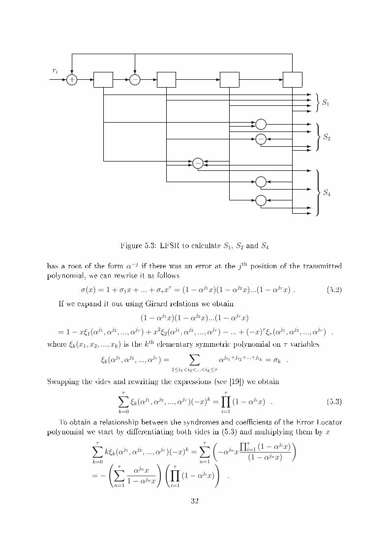
3. Thisallows us to extract S1, S2 and S4 from the circuit in Figure 5.1, as shown below
For a (15, 5, 7) BCH code, besides the circuit above, we also need a circuit to computeS3 and S6, and another one just to compute S5. Overall, we would need 3× 4 �ip-�ops,approximately 3 × 4 XORs for the multiplication circuits and 2 extra XORs for each ofthe 3 even syndromes. This gives us a total of 12 �ip-�ops and 18 XORs.
In a general case it is easy to see that we need tm �ip-�ops. The number of XORs ismore di�cult to estimate. For the LFSR circuit, we can assume that m XORs are usedfor each of the t circuits, and for the recombination of the LFSR outputs (forming theindividual syndromes) we estimate tm2
2XORs for all t circuits. These assumptions can be
made especially if we consider a slightly di�erent method for computing the syndromes,explained in Appendix B.2.
5.2.3 Finding the Error-Locator polynomial
The most complicated step in decoding a BCH code is �nding the Error-Locator poly-nomial σ(x). We �nd the Error-Locator polynomial by relating the coe�cients of σ(x)with the 2t syndromes we computed in the last step. Since the Error-Locator polynomial
31
- - - -� �� � ��- -+ +
? ?ri
----
}S1
--� ��
+ --
- �� ��+
--
S2
- �- �� ��
+-
- �� ��+
-
- �� ��+
--
S4
Figure 5.3: LFSR to calculate S1, S2 and S4
has a root of the form α−j if there was an error at the jth position of the transmittedpolynomial, we can rewrite it as follows
σ(x) = 1 + σ1x+ ...+ στxτ = (1− αj1x)(1− αj2x)...(1− αjτx) . (5.2)
If we expand it out using Girard relations we obtain
(1− αj1x)(1− αj2x)...(1− αjτx)
= 1− xξ1(αj1 , αj2 , ..., αjτ ) + x2ξ2(αj1 , αj2 , ..., αjτ )− ...+ (−x)τξτ (α
j1 , αj2 , ..., αjτ ) .
where ξk(x1, x2, ..., xk) is the kth elementary symmetric polynomial on τ variables
ξk(αj1 , αj2 , ..., αjτ ) =
∑1≤i1<i2<...<ik≤τ
αji1+ji2+...+jik = σk .
Swapping the sides and rewriting the expressions (see [19]) we obtain
τ∑k=0
ξk(αj1 , αj2 , ..., αjτ )(−x)k =
τ∏i=1
(1− αjix) . (5.3)
To obtain a relationship between the syndromes and coe�cients of the Error-Locatorpolynomial we start by di�erentiating both sides in (5.3) and multiplying them by x
τ∑k=0
kξk(αj1 , αj2 , ..., αjτ )(−x)k =
τ∑n=1
(−αjnx
∏τi=1 (1− αjix)
(1− αjnx)
)= −
(τ∑
n=1
αjnx
1− αjnx
)(τ∏i=1
(1− αjix)
).
32
By re-using expression (5.3) and developing the formal power series
= −
(τ∑
n=1
∞∑m=0
(αjnx)m
)(τ∑t=0
ξt(αj1 , αj2 , ..., αjτ )(−x)t
)
= −
(∞∑m=0
τ∑n=1
(αjnx)m
)(τ∑t=0
ξt(αj1 , ..., αjτ )(−x)t
)
=
(∞∑m=0
xmτ∑
n=1
αmjn
)(τ∑t=0
(−1)t+1ξt(αj1 , ..., αjτ )xt
) .
Now we can plug in the syndromes Sm and the coe�cients of the Error-Locatorpolynomial σk
τ∑k=0
(−1)k+1kσkxk =
(∞∑m=0
xmSm
)(τ∑t=0
(−1)t+1σtxt
). (5.4)
Finally, by comparing the coe�cient of xk on both sides of (5.4), we obtain the kth
Newton's identity as followss
(−1)k+1kσk =k∑t=1
(−1)k−t+1Stσk−t . (5.5)
where we assume that σi = 0 for i > τ . Since we are dealing with binary BCH codes, wecan disregard the signs and re-write the expression as follows
k∑t=1
Stσk−t + kσk = 0 . (5.6)
which yields the following list of relations
S1 + σ1 = 0
S2 + σ1S1 + 2σ2 = 0...
Sτ + σ1Sτ−1 + ...+ στ−1S1 + τστ = 0
Sτ+1 + σ1Sτ + ...+ στ−1S2 + στS1 = 0 (5.7)
Sτ+2 + σ1Sτ+1 + ...+ στ−1S3 + στS2 = 0
...
S2t + σ1S2t−1 + ...+ στ−1S2t+1−τ + στS2t−τ = 0 .
By looking at the last 2t − τ equations we see that �nding the coe�cients of the error-locating polynomial σ(x) is equivalent to looking for a linear recursion on the Si.
Sk =τ∑i=1
σiSk−i for k > τ (5.8)
For τ ≤ t there should be only one such linear recursion. It can be found via theBerlekamp-Massey algorithm.
33
5.2.4 The Berlekamp-Massey Algorithm
The Berlekamp-Massey Algorithm provides a polynomial-time algorithm to �nd the short-est linear recursion that generates a given stream. In other words, it allows us to �ndthe minimal polynomial (in our case, the Error-Locator polynomial) that generates arecurrent sequence. It is an iterative method, in which one checks if a trial polynomialσ(x) will generate the next output in the stream and, if not, applies a correction to it.The procedure is as follows:
We start with a polynomial σ(1)(x) that satis�es the �rst identity from (5.7). Thispolynomial can also be seen as just a list of coe�cients, since it will not be used asa polynomial in its proper sense during the steps of the algorithm. So we start withσ(1)(x) = S1x and σi = 0 for i > 1. Now we check to see if these coe�cients satisfy thesecond identity from (5.7). If they do, we set σ(2)(x) := σ(1)(x) and we move on to thenext identity. If not, we need to add a correction term to σ(1)(x) so that it satis�es thesecond identity. In general, at each iteration r, a new polynomial σ(r)(x) is produced. Ifthe coe�cients σ(r)(x) do not satisfy the r+ 1th identity, we �rst calculate how much therth discrepancy ∆r is
∆r = Sr+1 + σ1Sr + ...+ σr−1S2 + σrS1 + rσr (5.9)
In order to eliminate this discrepancy, we look at the previous iterations and �nd aσ(b)(x), for b < r whose discrepancy from the bth identity was also di�erent than 0. Thenwe normalize the polynomial with respect to its discrepancy ∆b, multiply it by our newdiscrepancy ∆r and shift its coe�cients up (or simply multiply it by a power of x) sothat its coe�cients, when added (or subtracted) to those of σ(r)(x), will eliminate thediscrepancy. In [1], Berlekamp proved that if we choose the most recent previous iterationin 2 deg(σ(r)(x)) < r (and ∆r 6= 0), this process yields the smallest-degree polynomialwhose coe�cients satisfy the r + 1th identity. Therefore, after 2t iterations, we obtainthe smallest-degree polynomial that satis�es all identities in (5.7), and thus we have ourError-Locator polynomial.
This iterative process can be systematically summarized in the following steps:
1. Set σ(1)(x) = 1 + S1x. This satis�es the �rst identity.
2. Then loop through the following steps until r = 2t.
3. Compute the discrepancy ∆r (from Equation (5.9))
• If ∆r = 0 set σ(r+1)(x) = σ(r)(x)
• If ∆r 6= 0 set σ(r+1)(x) := σ(r)(x) + xr−b∆r∆−1b σ(b)(x) where σ(b)(x), the
solution at iteration b, is the most recent solution such that ∆b 6= 0 and2 deg(σ(b)(x)) < b
Hardware implementation of Berlekamp-Massey's algorithm
The basic idea behind the hardware implementation for this iterative process is to noticethat, from one identity in (5.7) to the next one, the syndromes get shifted to the righton the coe�cients of σ(r)(x)). Therefore, we store the coe�cients of σ(r)(x)) in a register
34
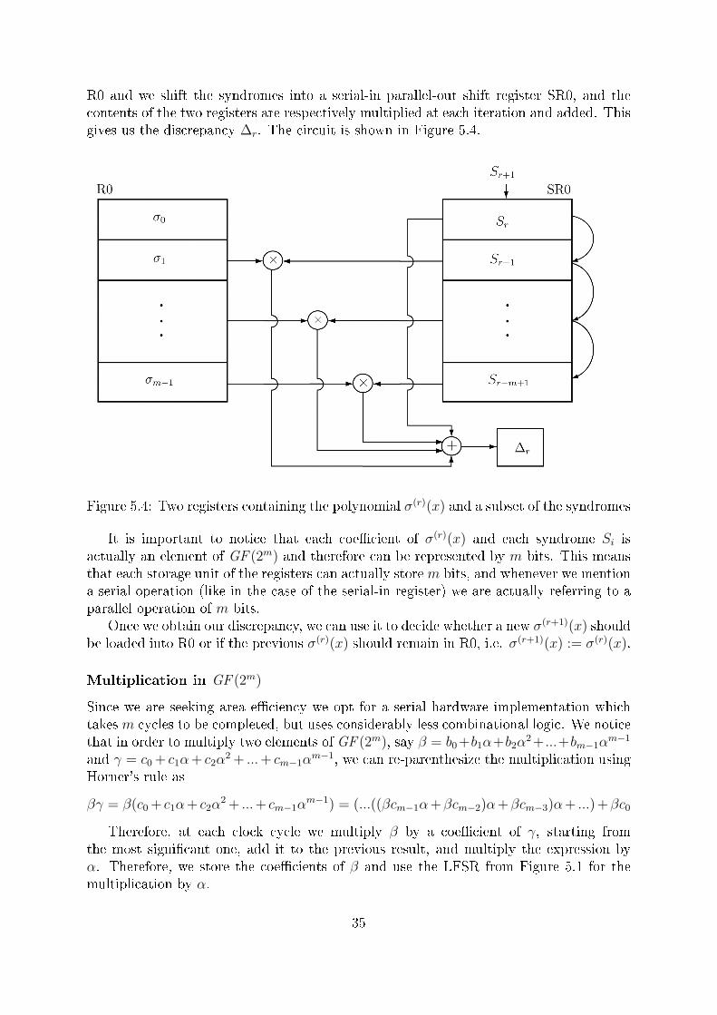
R0 and we shift the syndromes into a serial-in parallel-out shift register SR0, and thecontents of the two registers are respectively multiplied at each iteration and added. Thisgives us the discrepancy ∆r. The circuit is shown in Figure 5.4.
Figure 5.4: Two registers containing the polynomial σ(r)(x) and a subset of the syndromes
It is important to notice that each coe�cient of σ(r)(x) and each syndrome Si isactually an element of GF (2m) and therefore can be represented by m bits. This meansthat each storage unit of the registers can actually storem bits, and whenever we mentiona serial operation (like in the case of the serial-in register) we are actually referring to aparallel operation of m bits.
Once we obtain our discrepancy, we can use it to decide whether a new σ(r+1)(x) shouldbe loaded into R0 or if the previous σ(r)(x) should remain in R0, i.e. σ(r+1)(x) := σ(r)(x).
Multiplication in GF (2m)
Since we are seeking area e�ciency we opt for a serial hardware implementation whichtakes m cycles to be completed, but uses considerably less combinational logic. We noticethat in order to multiply two elements of GF (2m), say β = b0 +b1α+b2α
2 + ...+bm−1αm−1
and γ = c0 + c1α+ c2α2 + ...+ cm−1α
m−1, we can re-parenthesize the multiplication usingHorner's rule as
βγ = β(c0 + c1α+ c2α2 + ...+ cm−1α
m−1) = (...((βcm−1α+βcm−2)α+βcm−3)α+ ...) +βc0
Therefore, at each clock cycle we multiply β by a coe�cient of γ, starting fromthe most signi�cant one, add it to the previous result, and multiply the expression byα. Therefore, we store the coe�cients of β and use the LFSR from Figure 5.1 for themultiplication by α.
35
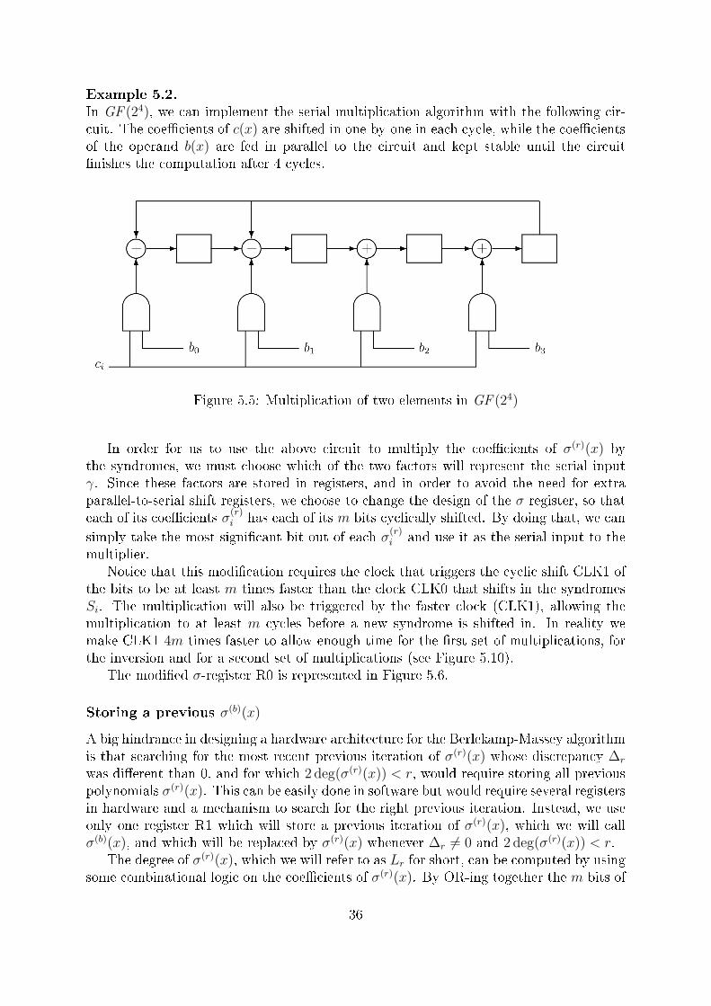
Example 5.2.In GF (24), we can implement the serial multiplication algorithm with the following cir-cuit. The coe�cients of c(x) are shifted in one-by-one in each cycle, while the coe�cientsof the operand b(x) are fed in parallel to the circuit and kept stable until the circuit�nishes the computation after 4 cycles.
Figure 5.5: Multiplication of two elements in GF (24)
In order for us to use the above circuit to multiply the coe�cients of σ(r)(x) bythe syndromes, we must choose which of the two factors will represent the serial inputγ. Since these factors are stored in registers, and in order to avoid the need for extraparallel-to-serial shift registers, we choose to change the design of the σ register, so thateach of its coe�cients σ
(r)i has each of its m bits cyclically shifted. By doing that, we can
simply take the most signi�cant bit out of each σ(r)i and use it as the serial input to the
multiplier.Notice that this modi�cation requires the clock that triggers the cyclic shift CLK1 of
the bits to be at least m times faster than the clock CLK0 that shifts in the syndromesSi. The multiplication will also be triggered by the faster clock (CLK1), allowing themultiplication to at least m cycles before a new syndrome is shifted in. In reality wemake CLK1 4m times faster to allow enough time for the �rst set of multiplications, forthe inversion and for a second set of multiplications (see Figure 5.10).
The modi�ed σ-register R0 is represented in Figure 5.6.
Storing a previous σ(b)(x)
A big hindrance in designing a hardware architecture for the Berlekamp-Massey algorithmis that searching for the most recent previous iteration of σ(r)(x) whose discrepancy ∆r
was di�erent than 0, and for which 2 deg(σ(r)(x)) < r, would require storing all previouspolynomials σ(r)(x). This can be easily done in software but would require several registersin hardware and a mechanism to search for the right previous iteration. Instead, we useonly one register R1 which will store a previous iteration of σ(r)(x), which we will callσ(b)(x), and which will be replaced by σ(r)(x) whenever ∆r 6= 0 and 2 deg(σ(r)(x)) < r.
The degree of σ(r)(x), which we will refer to as Lr for short, can be computed by usingsome combinational logic on the coe�cients of σ(r)(x). By OR-ing together the m bits of
36
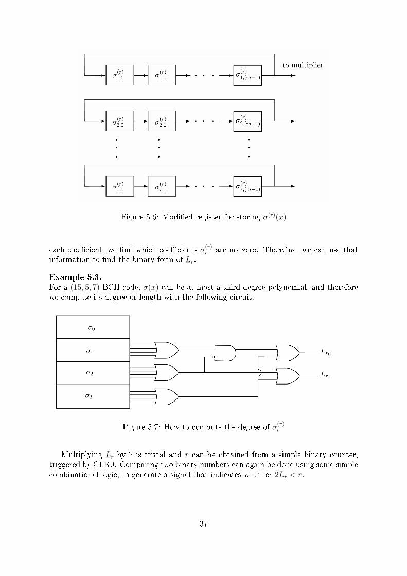
Figure 5.6: Modi�ed register for storing σ(r)(x)
each coe�cient, we �nd which coe�cients σ(r)i are nonzero. Therefore, we can use that
information to �nd the binary form of Lr.
Example 5.3.For a (15, 5, 7) BCH code, σ(x) can be at most a third degree polynomial, and thereforewe compute its degree or length with the following circuit.
Figure 5.7: How to compute the degree of σ(r)i
Multiplying Lr by 2 is trivial and r can be obtained from a simple binary counter,triggered by CLK0. Comparing two binary numbers can again be done using some simplecombinational logic, to generate a signal that indicates whether 2Lr < r.
37
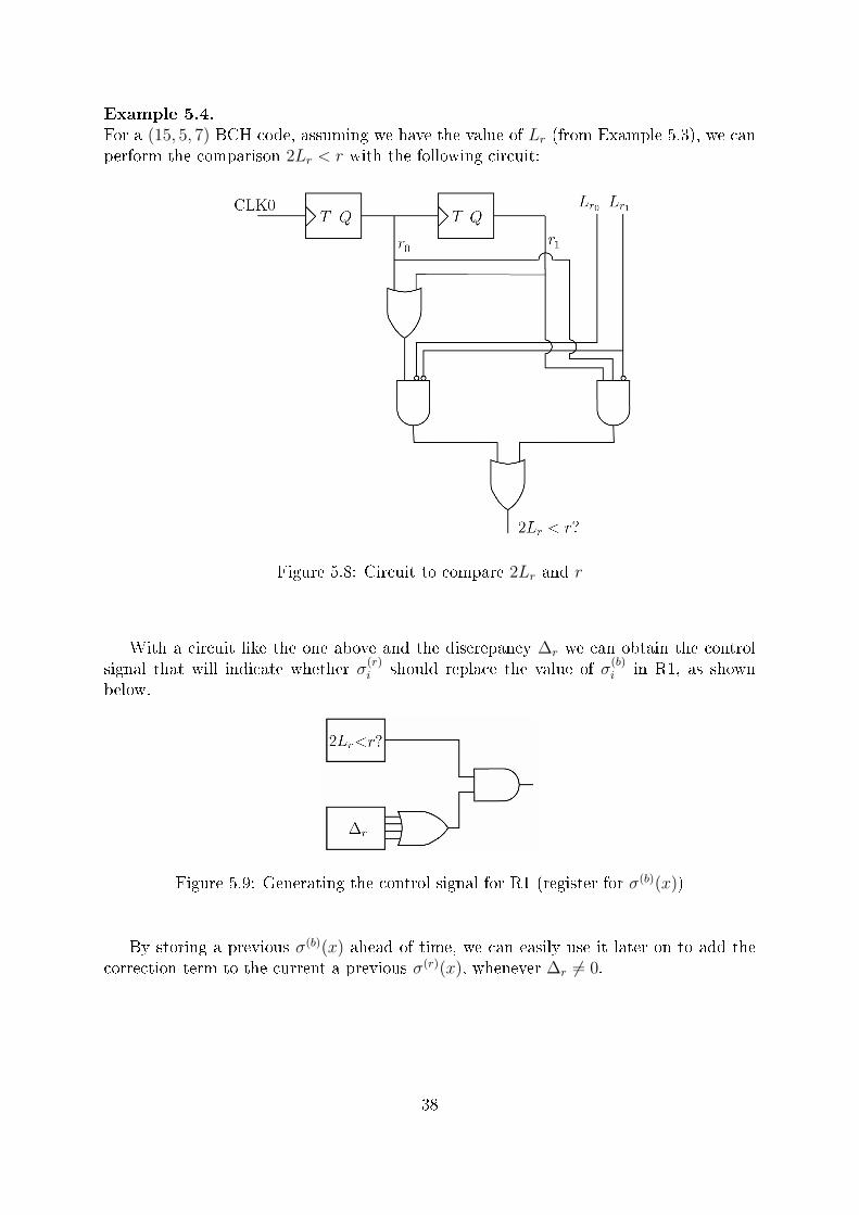
Example 5.4.For a (15, 5, 7) BCH code, assuming we have the value of Lr (from Example 5.3), we canperform the comparison 2Lr < r with the following circuit:
Figure 5.8: Circuit to compare 2Lr and r
With a circuit like the one above and the discrepancy ∆r we can obtain the controlsignal that will indicate whether σ
(r)i should replace the value of σ
(b)i in R1, as shown
below.
Figure 5.9: Generating the control signal for R1 (register for σ(b)(x))
By storing a previous σ(b)(x) ahead of time, we can easily use it later on to add thecorrection term to the current a previous σ(r)(x), whenever ∆r 6= 0.
38
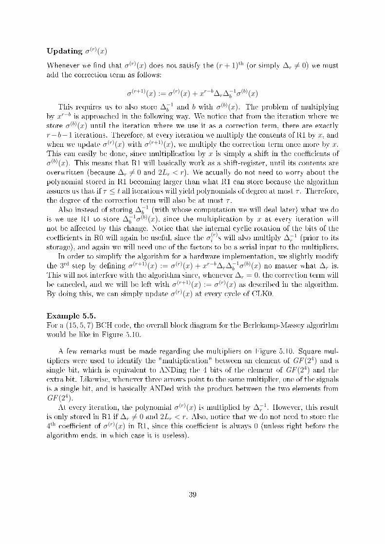
Updating σ(r)(x)
Whenever we �nd that σ(r)(x) does not satisfy the (r + 1)th (or simply ∆r 6= 0) we mustadd the correction term as follows:
σ(r+1)(x) := σ(r)(x) + xr−b∆r∆−1b σ(b)(x)
This requires us to also store ∆−1b and b with σ(b)(x). The problem of multiplying
by xr−b is approached in the following way. We notice that from the iteration where westore σ(b)(x) until the iteration where we use it as a correction term, there are exactlyr−b−1 iterations. Therefore, at every iteration we multiply the contents of R1 by x, andwhen we update σ(r)(x) with σ(r+1)(x), we multiply the correction term once more by x.This can easily be done, since multiplication by x is simply a shift in the coe�cients ofσ(b)(x). This means that R1 will basically work as a shift-register, until its contents areoverwritten (because ∆r 6= 0 and 2Lr < r). We actually do not need to worry about thepolynomial stored in R1 becoming larger than what R1 can store because the algorithmassures us that if τ ≤ t all iterations will yield polynomials of degree at most τ . Therefore,the degree of the correction term will also be at most τ .
Also instead of storing ∆−1b (with whose computation we will deal later) what we do
is we use R1 to store ∆−1b σ(b)(x), since the multiplication by x at every iteration will
not be a�ected by this change. Notice that the internal cyclic rotation of the bits of thecoe�cients in R0 will again be useful, since the σ
(r)i s will also multiply ∆−1
r (prior to itsstorage), and again we will need one of the factors to be a serial input to the multipliers.
In order to simplify the algorithm for a hardware implementation, we slightly modifythe 3rd step by de�ning σ(r+1)(x) := σ(r)(x) + xr−b∆r∆
−1b σ(b)(x) no matter what ∆r is.
This will not interfere with the algorithm since, whenever ∆r = 0, the correction term willbe canceled, and we will be left with σ(r+1)(x) := σ(r)(x) as described in the algorithm.By doing this, we can simply update σ(r)(x) at every cycle of CLK0.
Example 5.5.For a (15, 5, 7) BCH code, the overall block diagram for the Berlekamp-Massey algorithmwould be like in Figure 5.10.
A few remarks must be made regarding the multipliers on Figure 5.10. Square mul-tipliers were used to identify the "multiplication" between an element of GF (24) and asingle bit, which is equivalent to ANDing the 4 bits of the element of GF (24) and theextra bit. Likewise, whenever three arrows point to the same multiplier, one of the signalsis a single bit, and is basically ANDed with the product between the two elements fromGF (24).
At every iteration, the polynomial σ(r)(x) is multiplied by ∆−1r . However, this result
is only stored in R1 if ∆r 6= 0 and 2Lr < r. Also, notice that we do not need to store the4th coe�cient of σ(r)(x) in R1, since this coe�cient is always 0 (unless right before thealgorithm ends, in which case it is useless).
39
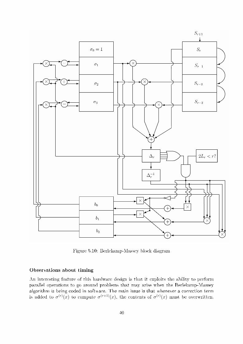
Figure 5.10: Berlekamp-Massey block diagram
Observations about timing
An interesting feature of this hardware design is that it exploits the ability to performparallel operations to go around problems that may arise when the Berlekamp-Masseyalgorithm is being coded in software. The main issue is that whenever a correction termis added to σ(r)(x) to compute σ(r+1)(x), the contents of σ(r)(x) must be overwritten.
40
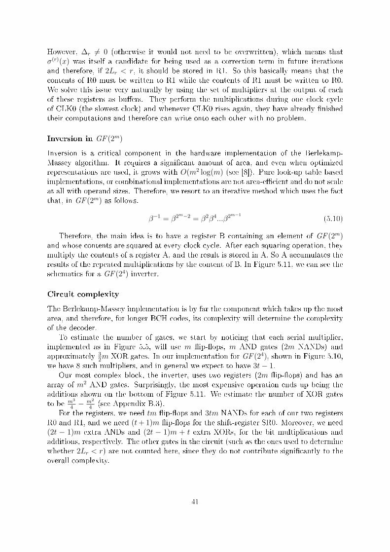
However, ∆r 6= 0 (otherwise it would not need to be overwritten), which means thatσ(r)(x) was itself a candidate for being used as a correction term in future iterationsand therefore, if 2Lr < r, it should be stored in R1. So this basically means that thecontents of R0 must be written to R1 while the contents of R1 must be written to R0.We solve this issue very naturally by using the set of multipliers at the output of eachof these registers as bu�ers. They perform the multiplications during one clock cycleof CLK0 (the slowest clock) and whenever CLK0 rises again, they have already �nishedtheir computations and therefore can write onto each other with no problem.
Inversion in GF (2m)
Inversion is a critical component in the hardware implementation of the Berlekamp-Massey algorithm. It requires a signi�cant amount of area, and even when optimizedrepresentations are used, it grows with O(m2 log(m) (see [8]). Pure look-up table basedimplementations, or combinational implementations are not area-e�cient and do not scaleat all with operand sizes. Therefore, we resort to an iterative method which uses the factthat, in GF (2m) as follows.
β−1 = β2m−2 = β2β4...β2m−1
(5.10)
Therefore, the main idea is to have a register B containing an element of GF (2m)and whose contents are squared at every clock cycle. After each squaring operation, theymultiply the contents of a register A, and the result is stored in A. So A accumulates theresults of the repeated multiplications by the content of B. In Figure 5.11, we can see theschematics for a GF (24) inverter.
Circuit complexity
The Berlekamp-Massey implementation is by far the component which takes up the mostarea, and therefore, for longer BCH codes, its complexity will determine the complexityof the decoder.
To estimate the number of gates, we start by noticing that each serial multiplier,implemented as in Figure 5.5, will use m �ip-�ops, m AND gates (2m NANDs) andapproximately 3
2m XOR gates. In our implementation for GF (24), shown in Figure 5.10,
we have 8 such multipliers, and in general we expect to have 3t− 1.Our most complex block, the inverter, uses two registers (2m �ip-�ops) and has an
array of m2 AND gates. Surprisingly, the most expensive operation ends up being theadditions shown on the bottom of Figure 5.11. We estimate the number of XOR gatesto be m3
4− m2
4(see Appendix B.3).
For the registers, we need tm �ip-�ops and 3tm NANDs for each of our two registersR0 and R1, and we need (t+ 1)m �ip-�ops for the shift-register SR0. Moreover, we need(2t − 1)m extra ANDs and (2t − 1)m + t extra XORs, for the bit multiplications andadditions, respectively. The other gates in the circuit (such as the ones used to determinewhether 2Lr < r) are not counted here, since they do not contribute signi�cantly to theoverall complexity.
41
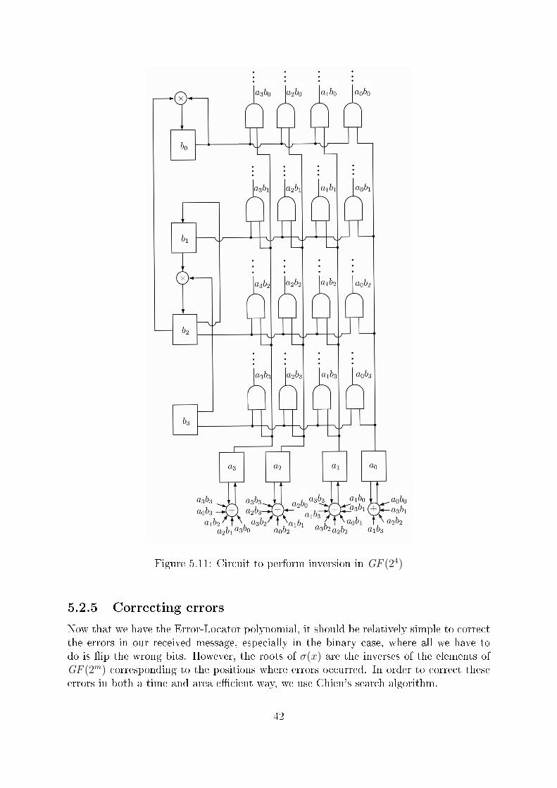
Figure 5.11: Circuit to perform inversion in GF (24)
5.2.5 Correcting errors
Now that we have the Error-Locator polynomial, it should be relatively simple to correctthe errors in our received message, especially in the binary case, where all we have todo is �ip the wrong bits. However, the roots of σ(x) are the inverses of the elements ofGF (2m) corresponding to the positions where errors occurred. In order to correct theseerrors in both a time and area e�cient way, we use Chien's search algorithm.
42
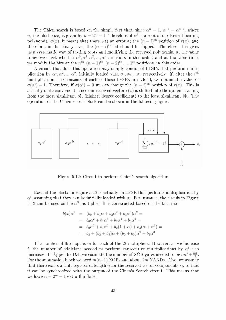
The Chien search is based on the simple fact that, since αn = 1, α−i = αn−i, wheren, the block size, is given by n = 2m − 1. Therefore, if αi is a root of our Error-Locatingpolynomial σ(x), it means that there was an error at the (n − i)th position of r(x), andtherefore, in the binary case, the (n − i)th bit should be �ipped. Therefore, this givesus a systematic way of testing roots and modifying the received polynomial at the sametime: we check whether α0, α1, α2, ..., αn are roots in this order, and at the same time,we modify the bits at the nth, (n− 1)th, (n− 2)th, ..., 1st positions, in this order.
A circuit that does this operation may simply consist of LFSRs that perform multi-plication by α1, α2, ..., ατ , initially loaded with σ1, σ2, ...στ respectively. If, after the ith
multiplication, the contents of each of these LFSRs are added, we obtain the value ofσ(αi) − 1. Therefore, if σ(αi) = 0 we can change the (n − i)th position of r(x). This isactually quite convenient, since our received vector r(x) is shifted into the system startingfrom the most signi�cant bit (highest degree coe�cient) to the least signi�cant bit. Theoperation of the Chien search block can be shown in the following �gure.
Figure 5.12: Circuit to perform Chien's search algorithm
Each of the blocks in Figure 5.12 is actually an LFSR that performs multiplication byαi, assuming that they can be initially loaded with σi. For instance, the circuit in Figure5.13 can be used as the α3 multiplier. It is constructed based on the fact that
b(x)α2 = (b0 + b1α + b2α2 + b3α
3)α2 =
= b0α2 + b1α
3 + b2α4 + b3α
5 =
= b0α2 + b1α
3 + b2(1 + α) + b3(α + α2) =
= b2 + (b2 + b3)α + (b0 + b3)α2 + b1α
3
The number of �ip-�ops is m for each of the 2t multipliers. However, as we increasei, the number of additions needed to perform consecutive multiplications by αi alsoincreases. In Appendix B.4, we estimate the number of XOR gates needed to bemt2+mt
2.
For the summation block we needm(t−1) XORs and about 2m NANDs. Also, we assumethat there exists a shift-register of length n for the received vector components ri, so thatit can be synchronized with the output of the Chien's Search circuit. This means thatwe have n = 2m − 1 extra �ip-�ops.
43
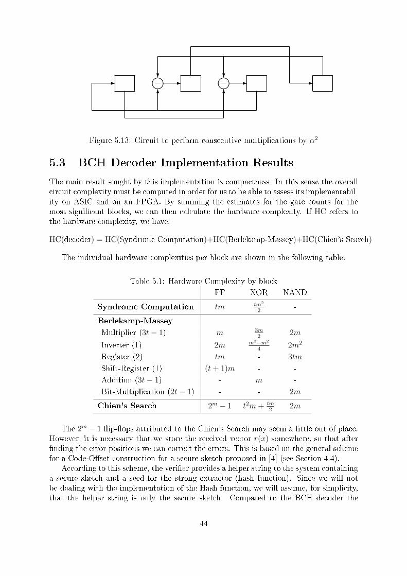
� �� � ��- - - -+ +
? ?
6 6
Figure 5.13: Circuit to perform consecutive multiplications by α2
5.3 BCH Decoder Implementation Results
The main result sought by this implementation is compactness. In this sense the overallcircuit complexity must be computed in order for us to be able to assess its implementabil-ity on ASIC and on an FPGA. By summing the estimates for the gate counts for themost signi�cant blocks, we can then calculate the hardware complexity. If HC refers tothe hardware complexity, we have:
HC(decoder) = HC(Syndrome Computation)+HC(Berlekamp-Massey)+HC(Chien's Search)
The individual hardware complexities per block are shown in the following table:
Table 5.1: Hardware Complexity by block
FF XOR NAND
Syndrome Computation tm tm2
2-
Berlekamp-Massey
Multiplier (3t− 1) m 3m2
2m
Inverter (1) 2m m3−m2
42m2
Register (2) tm - 3tm
Shift-Register (1) (t+ 1)m - -
Addition (3t− 1) - m -
Bit-Multiplication (2t− 1) - - 2m
Chien's Search 2m − 1 t2m+ tm2
2m
The 2m − 1 �ip-�ops attributed to the Chien's Search may seem a little out of place.However, it is necessary that we store the received vector r(x) somewhere, so that after�nding the error positions we can correct the errors. This is based on the general schemefor a Code-O�set construction for a secure sketch proposed in [4] (see Section 4.4).
According to this scheme, the veri�er provides a helper string to the system containinga secure sketch and a seed for the strong extractor (hash function). Since we will notbe dealing with the implementation of the Hash function, we will assume, for simplicity,that the helper string is only the secure sketch. Compared to the BCH decoder the
44
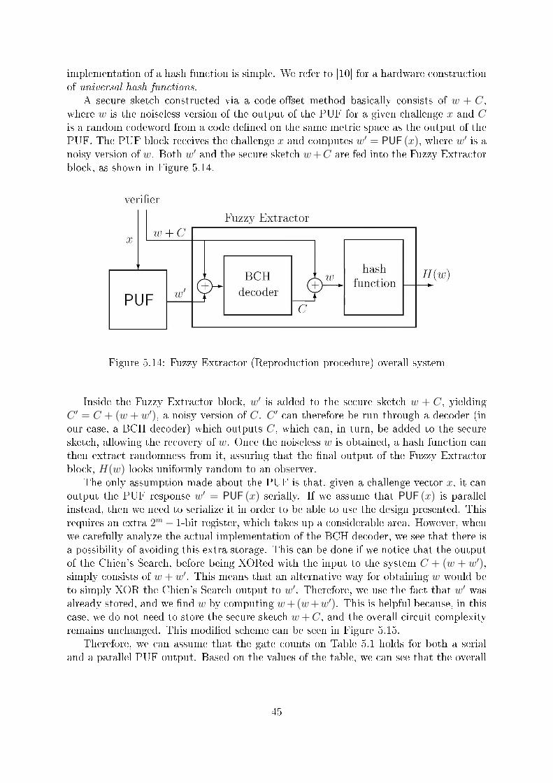
implementation of a hash function is simple. We refer to [10] for a hardware constructionof universal hash functions.
A secure sketch constructed via a code-o�set method basically consists of w + C,where w is the noiseless version of the output of the PUF for a given challenge x and Cis a random codeword from a code de�ned on the same metric space as the output of thePUF. The PUF block receives the challenge x and computes w′ = PUF (x), where w′ is anoisy version of w. Both w′ and the secure sketch w+C are fed into the Fuzzy Extractorblock, as shown in Figure 5.14.
Figure 5.14: Fuzzy Extractor (Reproduction procedure) overall system
Inside the Fuzzy Extractor block, w′ is added to the secure sketch w + C, yieldingC ′ = C + (w + w′), a noisy version of C. C ′ can therefore be run through a decoder (inour case, a BCH decoder) which outputs C, which can, in turn, be added to the securesketch, allowing the recovery of w. Once the noiseless w is obtained, a hash function canthen extract randomness from it, assuring that the �nal output of the Fuzzy Extractorblock, H(w) looks uniformly random to an observer.
The only assumption made about the PUF is that, given a challenge vector x, it canoutput the PUF response w′ = PUF (x) serially. If we assume that PUF (x) is parallelinstead, then we need to serialize it in order to be able to use the design presented. Thisrequires an extra 2m− 1-bit register, which takes up a considerable area. However, whenwe carefully analyze the actual implementation of the BCH decoder, we see that there isa possibility of avoiding this extra storage. This can be done if we notice that the outputof the Chien's Search, before being XORed with the input to the system C + (w + w′),simply consists of w + w′. This means that an alternative way for obtaining w would beto simply XOR the Chien's Search output to w′. Therefore, we use the fact that w′ wasalready stored, and we �nd w by computing w+ (w+w′). This is helpful because, in thiscase, we do not need to store the secure sketch w+C, and the overall circuit complexityremains unchanged. This modi�ed scheme can be seen in Figure 5.15.
Therefore, we can assume that the gate counts on Table 5.1 holds for both a serialand a parallel PUF output. Based on the values of the table, we can see that the overall
45
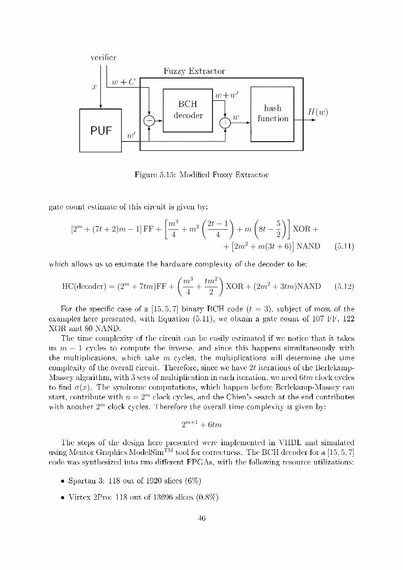
Figure 5.15: Modi�ed Fuzzy Extractor
gate count estimate of this circuit is given by:
[2m + (7t+ 2)m− 1] FF +
[m3
4+m2
(2t− 1
4
)+m
(8t− 5
2
)]XOR +
+[2m2 +m(3t+ 6)
]NAND (5.11)
which allows us to estimate the hardware complexity of the decoder to be:
HC(decoder) = (2m + 7tm)FF +
(m3
4+tm2
2
)XOR + (2m2 + 3tm)NAND (5.12)
For the speci�c case of a [15, 5, 7] binary BCH code (t = 3), subject of most of theexamples here presented, with Equation (5.11), we obtain a gate count of 107 FF, 122XOR and 80 NAND.
The time complexity of the circuit can be easily estimated if we notice that it takesus m − 1 cycles to compute the inverse, and since this happens simultaneously withthe multiplications, which take m cycles, the multiplications will determine the timecomplexity of the overall circuit. Therefore, since we have 2t iterations of the Berlekamp-Massey algorithm, with 3 sets of multiplication in each iteration, we need 6tm clock cyclesto �nd σ(x). The syndrome computations, which happen before Berlekamp-Massey canstart, contribute with n = 2m clock cycles, and the Chien's search at the end contributeswith another 2m clock cycles. Therefore the overall time complexity is given by:
2m+1 + 6tm
The steps of the design here presented were implemented in VHDL and simulatedusing Mentor Graphics ModelSimTM tool for correctness. The BCH decoder for a [15, 5, 7]code was synthesized into two di�erent FPGAs, with the following resource utilizations:
• Spartan 3: 118 out of 1920 slices (6%)
• Virtex 2Pro: 118 out of 13696 slices (0.8%)
46

These results show that this implementation is fairly reasonable in terms of FPGAusage. However, in order for this implementation to be useful, we must consider blocksizes of at least 100 bits (m ≥ 7). Considering the dominant term of our hardwarecomplexity to be m3 (which is reasonable for m < 10), this change would increase theFPGA usage by a factor of at most 8. This means that we should still be able to �t thedesign on a simple Spartan 3 board, although it would become impractical to use it inan FPGA IP protection setting.
47
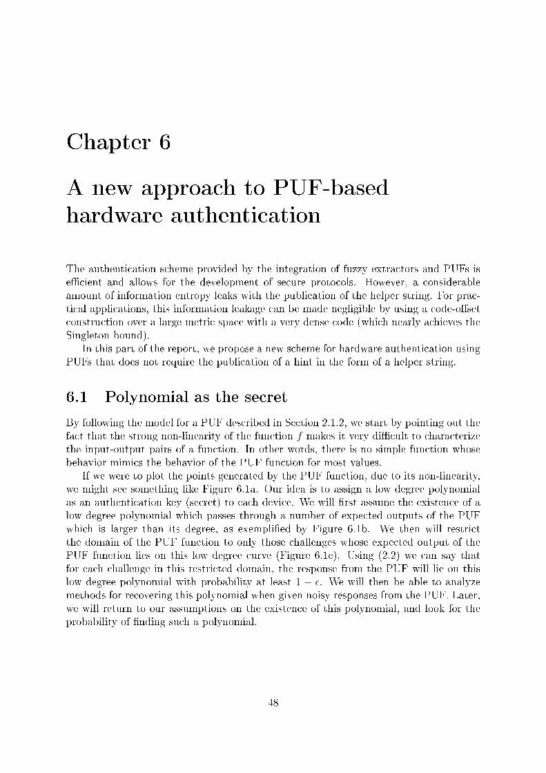
Chapter 6
A new approach to PUF-based
hardware authentication
The authentication scheme provided by the integration of fuzzy extractors and PUFs ise�cient and allows for the development of secure protocols. However, a considerableamount of information entropy leaks with the publication of the helper string. For prac-tical applications, this information leakage can be made negligible by using a code-o�setconstruction over a large metric space with a very dense code (which nearly achieves theSingleton bound).
In this part of the report, we propose a new scheme for hardware authentication usingPUFs that does not require the publication of a hint in the form of a helper string.
6.1 Polynomial as the secret
By following the model for a PUF described in Section 2.1.2, we start by pointing out thefact that the strong non-linearity of the function f makes it very di�cult to characterizethe input-output pairs of a function. In other words, there is no simple function whosebehavior mimics the behavior of the PUF function for most values.
If we were to plot the points generated by the PUF function, due to its non-linearity,we might see something like Figure 6.1a. Our idea is to assign a low degree polynomialas an authentication key (secret) to each device. We will �rst assume the existence of alow degree polynomial which passes through a number of expected outputs of the PUFwhich is larger than its degree, as exempli�ed by Figure 6.1b. We then will restrictthe domain of the PUF function to only those challenges whose expected output of thePUF function lies on this low degree curve (Figure 6.1c). Using (2.2) we can say thatfor each challenge in this restricted domain, the response from the PUF will lie on thislow degree polynomial with probability at least 1 − ε. We will then be able to analyzemethods for recovering this polynomial when given noisy responses from the PUF. Later,we will return to our assumptions on the existence of this polynomial, and look for theprobability of �nding such a polynomial.
48
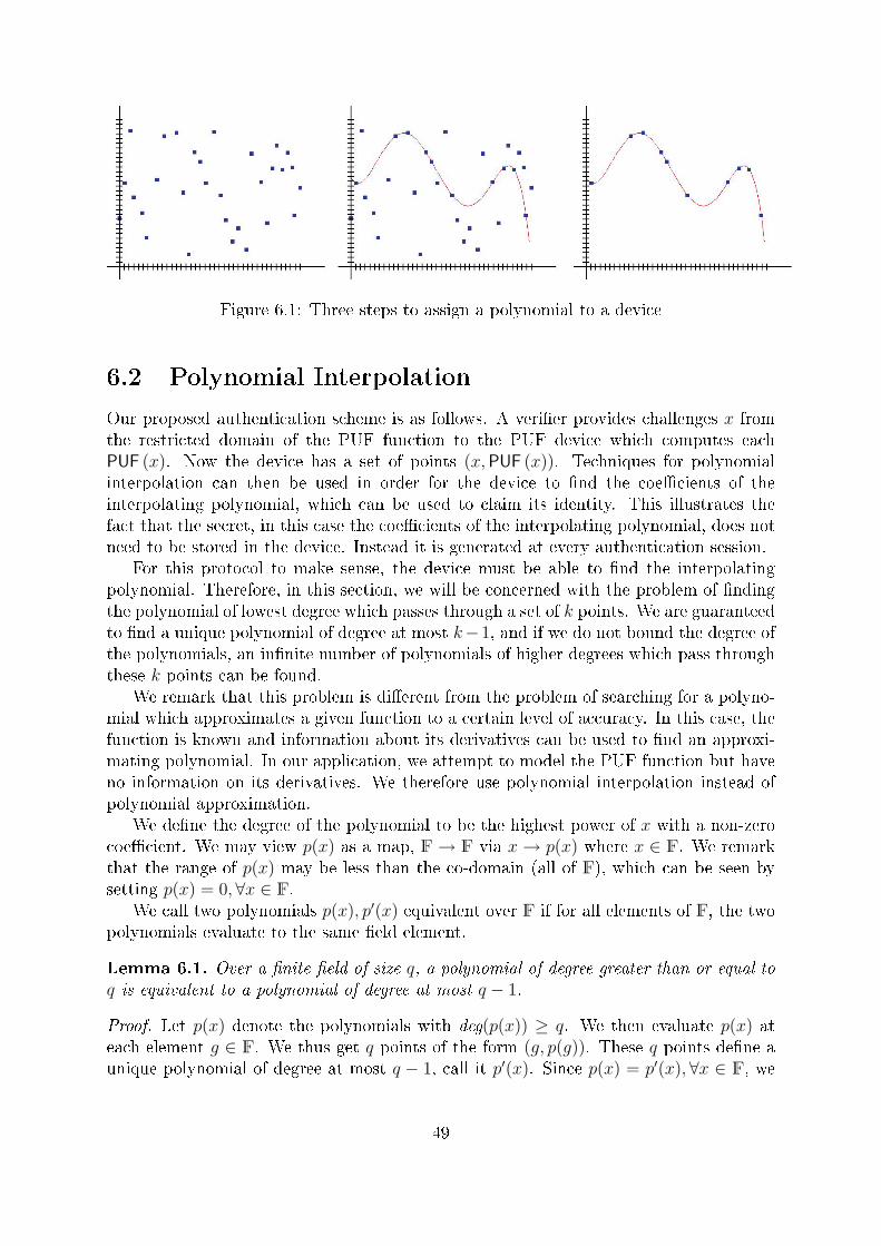
Figure 6.1: Three steps to assign a polynomial to a device
6.2 Polynomial Interpolation
Our proposed authentication scheme is as follows. A veri�er provides challenges x fromthe restricted domain of the PUF function to the PUF device which computes eachPUF (x). Now the device has a set of points (x,PUF (x)). Techniques for polynomialinterpolation can then be used in order for the device to �nd the coe�cients of theinterpolating polynomial, which can be used to claim its identity. This illustrates thefact that the secret, in this case the coe�cients of the interpolating polynomial, does notneed to be stored in the device. Instead it is generated at every authentication session.
For this protocol to make sense, the device must be able to �nd the interpolatingpolynomial. Therefore, in this section, we will be concerned with the problem of �ndingthe polynomial of lowest degree which passes through a set of k points. We are guaranteedto �nd a unique polynomial of degree at most k−1, and if we do not bound the degree ofthe polynomials, an in�nite number of polynomials of higher degrees which pass throughthese k points can be found.
We remark that this problem is di�erent from the problem of searching for a polyno-mial which approximates a given function to a certain level of accuracy. In this case, thefunction is known and information about its derivatives can be used to �nd an approxi-mating polynomial. In our application, we attempt to model the PUF function but haveno information on its derivatives. We therefore use polynomial interpolation instead ofpolynomial approximation.
We de�ne the degree of the polynomial to be the highest power of x with a non-zerocoe�cient. We may view p(x) as a map, F→ F via x→ p(x) where x ∈ F. We remarkthat the range of p(x) may be less than the co-domain (all of F), which can be seen bysetting p(x) = 0,∀x ∈ F.
We call two polynomials p(x), p′(x) equivalent over F if for all elements of F, the twopolynomials evaluate to the same �eld element.
Lemma 6.1. Over a �nite �eld of size q, a polynomial of degree greater than or equal toq is equivalent to a polynomial of degree at most q − 1.
Proof. Let p(x) denote the polynomials with deg(p(x)) ≥ q. We then evaluate p(x) ateach element g ∈ F. We thus get q points of the form (g, p(g)). These q points de�ne aunique polynomial of degree at most q − 1, call it p′(x). Since p(x) = p′(x),∀x ∈ F, we
49
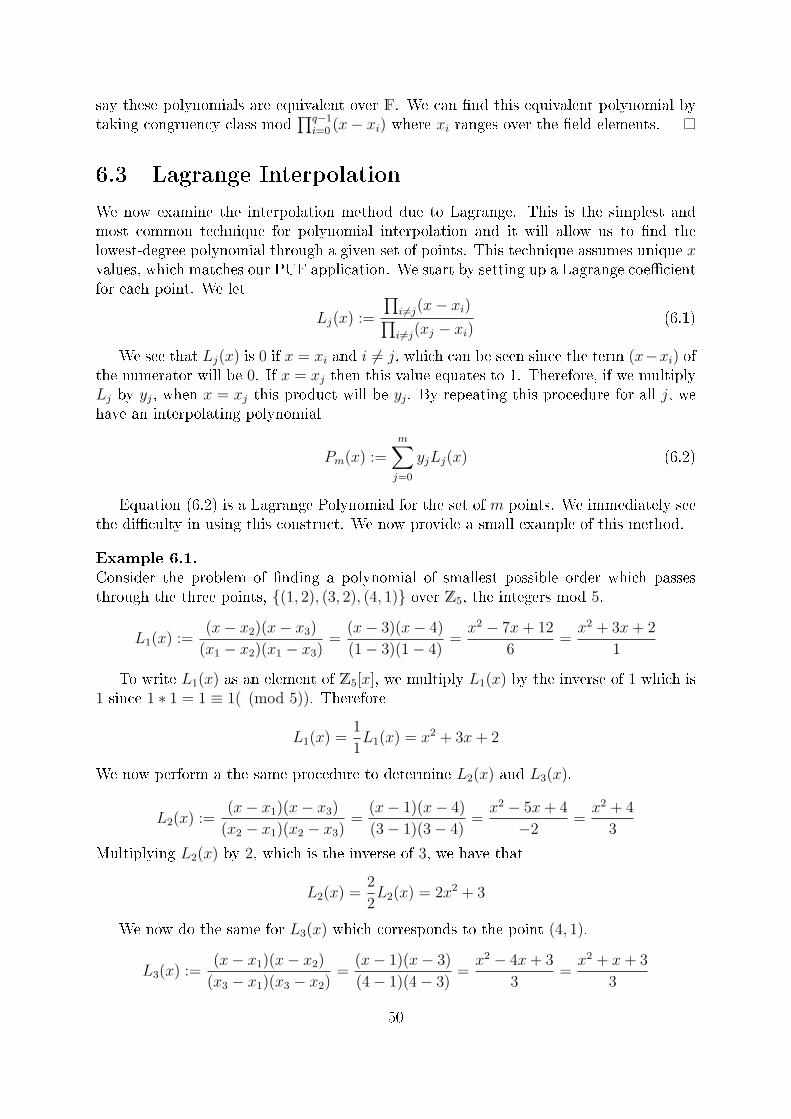
say these polynomials are equivalent over F. We can �nd this equivalent polynomial bytaking congruency class mod
∏q−1i=0 (x− xi) where xi ranges over the �eld elements.
6.3 Lagrange Interpolation
We now examine the interpolation method due to Lagrange. This is the simplest andmost common technique for polynomial interpolation and it will allow us to �nd thelowest-degree polynomial through a given set of points. This technique assumes unique xvalues, which matches our PUF application. We start by setting up a Lagrange coe�cientfor each point. We let
Lj(x) :=
∏i 6=j(x− xi)∏i 6=j(xj − xi)
(6.1)
We see that Lj(x) is 0 if x = xi and i 6= j, which can be seen since the term (x−xi) ofthe numerator will be 0. If x = xj then this value equates to 1. Therefore, if we multiplyLj by yj, when x = xj this product will be yj. By repeating this procedure for all j, wehave an interpolating polynomial
Pm(x) :=m∑j=0
yjLj(x) (6.2)
Equation (6.2) is a Lagrange Polynomial for the set of m points. We immediately seethe di�culty in using this construct. We now provide a small example of this method.
Example 6.1.Consider the problem of �nding a polynomial of smallest possible order which passesthrough the three points, {(1, 2), (3, 2), (4, 1)} over Z5, the integers mod 5.
L1(x) :=(x− x2)(x− x3)
(x1 − x2)(x1 − x3)=
(x− 3)(x− 4)
(1− 3)(1− 4)=x2 − 7x+ 12
6=x2 + 3x+ 2
1
To write L1(x) as an element of Z5[x], we multiply L1(x) by the inverse of 1 which is1 since 1 ∗ 1 = 1 ≡ 1( (mod 5)). Therefore
L1(x) =1
1L1(x) = x2 + 3x+ 2
We now perform a the same procedure to determine L2(x) and L3(x).
L2(x) :=(x− x1)(x− x3)
(x2 − x1)(x2 − x3)=
(x− 1)(x− 4)
(3− 1)(3− 4)=x2 − 5x+ 4
−2=x2 + 4
3
Multiplying L2(x) by 2, which is the inverse of 3, we have that
L2(x) =2
2L2(x) = 2x2 + 3
We now do the same for L3(x) which corresponds to the point (4, 1).
L3(x) :=(x− x1)(x− x2)
(x3 − x1)(x3 − x2)=
(x− 1)(x− 3)
(4− 1)(4− 3)=x2 − 4x+ 3
3=x2 + x+ 3
3
50
Therefore
L3(x) =2
2L3(x) = 2x2 + 2x+ 1
We now create our interpolating polynomial as shown in Equation (6.2)
P3(x) :=3∑j=0
yjLj(x) = 2L1(x) + 2L2(x) + 1L3(x)
P3(x) = (2x2 + x+ 4) + (4x2 + 1) + (2x2 + 2x+ 1) = 3x2 + 3x+ 1
P3(1) = (3 + 3 + 1) = 2 (mod 5)
P3(3) = (27 + 9 + 1) = 2 (mod 5)
P3(4) = (48 + 12 + 1) = 1 (mod 5)
We have that the three points match and hence this P3(x) interpolates the points.During the construction, we could make sure we were construction the Lj(x) correctly. Forexample, we could check L2(x) and make sure L2(1) = 2(1)+3 = 0 , L2(4) = 2(16)+3 = 0and L2(3) = 2(9) + 3 = 1. This shows the term L2(x) is the only term that contributesto P3(x) when x = 3, which corresponds to our second point.
6.3.1 Restrictions on Lagrange Interpolation
A major drawback to Lagrange Interpolation is its inability to handle noise. In theconstruction, we create polynomials Li which correspond to a speci�c x value. If thesex values are known, as will be the case with our protocol, the errors, or the noise, mayonly be present in the y values. There is no built in error-correcting mechanism that willallow for the detection of an incorrect y value. If there was additional information, suchas the degree of the lowest-degree polynomial that passes through k points, then there isan obvious procedure that can be used to �nd such a polynomial. For example, supposewe are looking for an interpolating polynomial for all k points with degree at most k− 2(extra information). We proceed by selecting all k subsets of size k − 1, and looking forthe lowest degree polynomial that goes through them. Then for each polynomial one cancheck how many points it goes through. This procedure becomes tedious and expensive asthe di�erence between the number of points and the degree of the polynomial increases.This however, motivates the search for algorithms which �nd such a polynomial quicklygiven points which may have incorrect y values. We will now present two approaches tothis problem, which we will refer to as polynomial interpolation �with lies�.
6.4 Polynomial interpolation �with lies�
The method provided by Lagrange Interpolation is a straightforward way of obtaining thelowest degree polynomial that goes through a set of points. However, when we considerthe setting where some of those points are misplaced or, in other words, there is noise inthe data, it can do very little for us.
51
When we consider the fact that for one to perform Lagrange Interpolation and �nda polynomial of degree at most d, all we need are d+ 1 points of the actual polynomial,it is intuitive to think that the introduction of some redundancy in the data points couldpossibly help us �nd the original polynomial, even in the presence of noise. For example,if instead of only d + 1 points we have d + 1 + r points, then, even if there are up tor misplaced data points, we should still be able to �nd a subset of d + 1 correct pointsthat allow us to recover the original polynomial via Lagrange Interpolation. Nonetheless,this method requires us to check at most
(d+1+rd+1
)possible sets of d + 1 points. Other
methods must be introduced in order to allow for a more e�cient way to �nd the actualpolynomial.
Interpolating with the aid of the Discrete Fourier Transform
From the comparison between the problem of recovering a polynomial when the datapoints have some noise and the problem of transmitting information over a noisy channelcomes the idea of applying solutions from the �eld of communications to polynomialrecovery.
In a communication system, a common way to �prepare� the information for trans-mission and for the addition of noise is to prede�ne a transmission bandwidth. This way,the receiver �knows� where to look for the information. Similarly, for the polynomialrecovery problem, we will only send nonzero information for a �nite set of frequencies, ora bandwidth.
More speci�cally, if we have a polynomial p(x) of degree k < q − 1 over GF (q), wewill evaluate this polynomial at n = q− 1 �consecutive� points of GF (q), α0, α1, ..., αn−1,where α is any primitive element of GF (q). Once each Vi = αi is transmitted, with somenoise added to it, the receiver may regard it as the coe�cients of another polynomialV (x), of degree n − 1. This is equivalent to the Discrete Fourier Transform on a �nite�eld (see Section 3.4.2).
The Discrete Fourier Transform when applied to �nite �elds demonstrates the dualitybetween the points on a polynomial and its coe�cients. Simply put, the coe�cients of ourinitial polynomial p(x), when multiplied by n will yield the values of V (αi), except that inreverse order. Since k < q− 1, the last few coe�cients of p(x), namely vk+1, vk+2, ..., vn−1
can all be regarded as 0. This yields an important result: if p(x) has degree at mostk, then V (αi) = 0 if i ≤ n − k. This can be interpreted as having a �nite bandwidthcontaining information. If we have nonzero data at those points, we must be dealing withnoise. This can be better understood with the following example.
52
Example 6.2.Consider the polynomial p(x) = 3 + 2x + x2 over Z7. By picking α = 3 (since |3| = 6),we calculate the each Vi = p(αi), as shown below in Table 6.4.
αi 30 = 1 31 = 3 32 = 2 33 = 6 34 = 4 35 = 5
Vi = p(αi) 6 4 4 2 6 3
This allows us to form the polynomial V (x) = 6 + 4x + 4x2 + 2x3 + 6x4 + 3x5. Wenow evaluate it at αi, for α = 1, 2, ..., n:
αi 31 = 3 32 = 2 33 = 6 34 = 4 35 = 2 36 = 1
V (αi) 0 0 0 6 5 4
Notice that 6 · p(x) = 4 + 5x + 6x2 + 0x3 + 0x4 + 0x5, which exempli�es the dualitybetween values of the polynomial when evaluated at certain points and its coe�cients.
In general, if a polynomial p(x) of degree at most k is evaluated at αi, for i =0, 1, 2, ..., n−1, and this information is transmitted via a noisy channel, one can build thepolynomial V (x) and evaluate it at αi, for i = 1, 2, ..., n, and check whether V (αi) = 0 fori = 1, 2, ..., n− k. In this case, there are two possibilities: either the values of p(x) werecorrectly transmitted or enough points were incorrectly transmitted to make it look likeanother polynomials of degree k was transmitted. One can easily show that the lattercase is only possible if n − k or more of the points were incorrectly transmitted, and ingeneral, we will assume the former case.
If V (αi) 6= 0 for some i, 1 ≤ i ≤ n− k, it is guaranteed that some of the points wereincorrectly transmitted. In this case, we simply assume that the received vector was:
V ′(x) = V (x) + e(x) (6.3)
where e(x) = e0 + e1x + ... + en−1xn−1 is the error vector. Now, if we evaluate this
received polynomial at each αi, 1 ≤ i ≤ n− k, we use the fact that V (αi) = 0 to obtainthe following equations:
V ′(α) = e0 + e1α + ...+ en−1αn−1
V ′(α2) = e0 + e1α2 + ...+ en−1α
2(n−1)
...
V ′(αn−k) = e0 + e1α3 + ...+ en−1α
3(n−1)
And we need to solve the following system:
1 α α2 α3 · · · αn−1
1 α2 α4 α6 · · · α2(n−1)
1 α3 α6 α9 · · · α3(n−1)
.... . .
...1 αn−k α2(n−k) α3(n−k) · · · α(n−k)(n−1)
e0e1...
en−1
=
V (α)V (α2)
...V (αn−k)
(6.4)
53
This systems has a large number of solutions, and therefore is not helpful. By assumingthat we only had up to n−k errors, we can then simplify the matrix in Equation (6.4) toa (n− k)× (n− k) matrix, which would yield a unique solution. However, for any choiceof n − k positions for the errors we would obtain a (possibly) di�erent solution, givingus a total of
(n
n− k
)=(nk
)solutions. If we assume that we had exactly t errors, there will
be(
n− tn− k − t
)=(n− tk
)possible combinations of n − k error positions that will give us the
right solution. In [16], it is shown that a �wrong� solution to this system can be given byat most
(t+k−1k
)choices of the n− k error positions. Therefore, in order for a �majority�
argument to work here, we must have(t+k−1k
)<(n−tk
)which implies that we must have
t+ k − 1 < n− t⇒ t <n− k + 1
2.
Therefore, we can recover our original polynomial if we have up to bn−k2c wrong data
points. In the next section, we consider another method for performing polynomial inter-polation with lies: Sudan's list-decoding algorithm. This new method has the advantagethat it does not require the number of errors to be at most bn−k
2c.
6.5 Sudan's algorithm
In this section we consider Sudan's randomized algorithm for constructing a list of allunivariate polynomials in the variable x of degree at most δ over F which agree with aset of n points from F2 in at least τ places. Moreover, if certain constraints are met, thisalgorithm runs in polynomial time in n. We �rst de�ne and describe the necessary inputto the algorithm. We then provide the algorithm, followed by more detailed analysis. Wefollow the approach in [17] closely.
Weighted degree of a polynomial [17]
For weights wx, wy ∈ Z+, the (wx, wy) weighted degree of a monomial qijxiyj is iwx+jwy.
The (wx, wy) weighted degree of a polynomial Q(x, y) =∑
ij qijxiyj is the maximum,
over the monomials with non, zero coe�cients, of the (wx, wy) weighted degree of themonomial.
Example 6.3.Consider the monomial
M(x, y) := 3x2y4
The (1, 3) weighted degree of this monomial is 2 · 1 + 3 · 4 = 14.If we knew y corresponded to the polynomial x2 +4x+1 then we would most likely be
interested in the (1, 2) weighted degree ofM(x, y) since y is a degree 2 function of x. If weknew or were searching for a degree at most ζ polynomial, then we would be interestedin the (1, ζ) weighted degree. The (1, 2) weighted degree of M(x, y) is 2 · 1 + 4 · 2 = 10.The (1, 2) weighted degree of the polynomial
p(x, y) := xy2 + x6 + 3
54
is equal to
max{(1 · 1 + 2 · 2
),(6 · 1 + 0 · 2
),(0 · 1 + 0 · 2
)} = max
{5, 6, 0
}= 6
Input points
The algorithm takes as inputs n points from F2. De�ne the set of these points as
A :={
(x1, y1), (x2, y2), ..., (xn, yn)}
The algorithm �nds all degree δ or less polynomials which agree with A in at least τplaces. In other words, it �nds all polynomials p(x) such that∣∣∣∣∣{(xi, yi) : f(xi) = yi and (xi, yi) ∈ A
}∣∣∣∣∣ ≥ τ
For the particular purpose of our algorithm, we do not allow repeated xi. We remarkthat this restriction is also the case if this algorithm is used for Reed Solomon decoding.
Example 6.4.Let F := Z7 be equal to the integers mod 7. Let n = 3 and let A := {(1, 3), (3, 2), (4, 5)}.Since there are no repeated x values, A is a valid point set. We do not allow A :={(1, 2), (1, 3), (4, 5)} since there are two points {(1, 2), (1, 3)} with the same x value.
6.5.1 Sudan's algorithm procedure [17]
Inputs:
n, δ, τ,{
(x1, y1), ..., (xn, yn)}
Parameters:
Parameters l, m to be set later
Find Q(x, y):
Find any function Q : F2 → F satisfying:
Q(x, y) has (1, δ) weighted degree at most m+ lδ∀i ∈ [n],Q(xi, yi) = 0Q is not identically zero.
}(6.5)
Factor Q(x, y):
Factor the polynomial Q(x, y) into irreducible factors.
55
Output polynomials:
Output all the polynomials f such that (y − f(x)) is a factor of Q and f(xi) = yi for atleast τ values of i from [n]
We remark that Sudan's algorithm does not work on any general code, as the necessaryconditions will not be met. We have the asymptotic condition τ ≥
√2nd, which generally
means this algorithm works better for low rate codes. In general this means that if thealgorithm is to return a low degree polynomial, it will have to agree with the initial pointsfor a large number of x values. We now proceed to analyze the algorithm, and later wewill analyze our implementation in maple.
6.5.2 The polynomial Q(x, y)
Q(x, y) is composed of terms of the form qkjxkyj. More speci�cally
Q(x, y) :=l∑
j=0
m+(l−j)d∑k=0
qkjxkyj (6.6)
We remark that l is the maximum power of y, and that m+ lδ is the maximum power ofx.
Number of coe�cients
In [17], it is claimed that the number of coe�cients of Q(x, y) is (m+ 1)(l + 1) + δ(l+12
)Proof.
l∑j=0
m+(l−j)d∑k=0
qkjxkyj =
l∑j=0
m∑k=0
qkjxkyj +
l∑j=0
m+(l−j)d∑k=m+1
qkjxkyj (6.7)
The �rst summation on the right hand side contributes (m + 1)(δ + 1) to the numberof coe�cients. For the second summation on the right hand side, we use a change ofvariables letting r = k−m. When k = m+ 1 we have that r = 1. When k = m+ (l− j)δwe have that r = (l − j)δ. Therefore we can right the second summation as
l∑j=0
(l−j)d∑k=1
q(r+m)jxr+myj
We can pull out the δ from the bound on the inner summation and then multiply theresulting number of coe�cients by δ. We are only interested in the number of coe�cients,and not the subscripts of q. When looking at the number of coe�cients we have l + (l−1)+(l−2)+ ...+(l− (l−1)+1)+(l− l+1) which is the sum of the �rst l numbers, whichis(l+12
). We multiply this number by δ to get the total contribution from the second
summation of the left hand side of (6.7). By summing the contributions from the �rstand second summations of the right hand side of (6.7), we have the claimed number ofcoe�cients, (m+ 1)(l + 1) + δ
(l+12
).
56
Claim 6.1. If a function Q : F2 → F satisfying (6.5) exists, the one can be found intime poly(n).
Proof. [17] Consider the coe�cient matrix with columns corresponding to the terms of Qde�ned above, and the rows corresponding to the input points from F2. We wish to �ndthe coe�cients qkj which satisfyQ(x, y) = 0 ∀i ∈ [n]. This is solving a linear homogeneousequation which can be done in polynomial time with row reducing the coe�cient matrix.We remark that we are not interested in the trivial solution, all qkj = 0 since then Q(x, y)would be identically zero.
Claim 6.2. If Q(x, y) is a function satisfying (6.5) and f(x) is a polynomial whichagrees with A in at least τ places and τ > m+ lδ then (y − f(x)) divides Q(x, y).
Proof. As given in [17], we argue Q(x, y) has weighted degree at most m + lδ. This isguaranteed through the de�nition of Q(x, y). We then consider Q(x, y) to be Q(x, f(x)).Since t > m + δ, Q(x, f(x)) has more zeros (t) than its degree, and must be identicallyzero. We then consider Q(x, y) to be a polynomial in y with coe�cients from F [x]. Bythe polynomial remainder theorem, we have that if Qx(ξ) = 0 then (y−ξ)) divides Qx(y).We then replace ξ with f(x).
Theorem 6.1. [17] The algorithm given will run in time polynomial in n given that
τ ≥ δ
⌈√2(n+ 1)
δ
⌉−⌊δ
2
⌋Proof. See [17].
Setting m and l
To ful�ll the algorithm requirements, the following parameters m and l can be set to (6.8)and (6.9) respectively (see [17]). (6.10) is used in the proof of showing Q(x, y) has morezeros than its degree and must be identically zero. (6.11) is used to guarantee polyno-mial implementation. Recall that with the algorithm Berlekamp and Welch, polynomialimplementation is guaranteed if τ ≥ n+δ
2, which is the error correction bound of the Reed
Solomon codes. This algorithm only returns at most one result. The asymptotic behaviorof (6.11) is
√2δn but has since been improved to
√δn (see [18]).
m :=
⌈δ
2
⌉− 1 (6.8)
l :=
⌈√2(n+ 1)
δ
⌉− 1 (6.9)
τ > m+ lδ (6.10)
τ ≥ δ
⌈√2(n+ 1)
δ
⌉−⌊δ
2
⌋(6.11)
57
Example 6.5.For example, if we are looking for a degree at most 10 polynomial, we have δ := 10. Letus assume that we have 30 := n points. Then
l :=
⌈√2(30 + 1)
10
⌉− 1 = 2
m :=
⌈10
2
⌉− 1 = 4
For restriction (6.10) we need τ > 4 + 2 · 10 which means we need at least 25 points outof 30 to match. For (6.11) we also need τ ≥ 25. This provides a brief example in thestrict requirements upon the inputs, which limits its practicability. The algorithm is bestsuited for when δ
nis small.
We now slightly modify the parameters and compare the amount of errors whichthese new parameters can tolerate. We let 19 := n points, and we are searching fora degree at most 10 := δ polynomial, we have l = 1 and m = 4 and hence we needt ≥ max(4 + 1 · 10, 10 · 2 − 5) = 15. Therefore, in order to be guaranteed a solutionin polynomial time from Sudan's Algorithm, there needs to exists a degree at most 10polynomial that agrees with the 19 points in at least 15 places.
6.5.3 Polynomially many solutions
In order for Sudan's algorithm to be implemented in polynomial time, the number of solu-
tions which it outputs needs to be polynomially bounded. In [17], if τn≥(√
2 + δ4n
√δn
)−
δ2n
then the number of polynomial returned by Sudan's algorithm is at most b τδ
+ 12−√
( τδ
+ 12)2 − 2n
δc ≤ 2n
τ+ δ2
We now quickly look at the more general problem of the number of polynomials whichare within a certain distance of an element in the metric space. We will follow [18]. Forevery c, we let ec(n, k, d, q) be a function such that for every (n, k)q code C of distancedis (C) = d, and for every received word r, there are at most (qn)c codewords in theHamming ball of radius e around r.
The case c = 0 corresponds to only having one codeword in the Hamming ball of someradius e around any element. For c = 0 this is just the error correcting radius of the codeand we let e = d−1
c.
We now examine the case when c = 2.
Theorem 6.2. [18] Let n, k, d, q, e satisfy d ≤ n′ and e < (1 −√
1− dn′
)n′ where n′ =
(1 − 1q)n. Then for every (n, k)q code C with dis (C) ≥ d and for every received word
r, there are at most qn2 codewords within a Hamming distance e from r. This is ageneralization of the Johnson bound.
6.5.4 Factoring Polynomials
In this section we will present the �rst few steps of Lenstra's algorithm (see [11]) to factorbivariate polynomials over �nite �elds. We will look at (x+2y)(x+3) over Z5. We de�ne
58
f = x2 + 2xy + 3x + 6y ∈ F[x, y], and notice that it is square free. We let δXf and δY fdenote the maximum degree of f in X and Y respectively. We have that δXf = 2 andδY f = 1.
Finding (Y − s)
We now need to �nd a suitable s ∈ Fq such that f mod (Y − s) = f(X, s) ∈ Fq[x]remains square-free. We write f as (2x+ 6)y+ (x2 + 3x), which can be done by collectingthe coe�cients of the varying degrees of y. We now wish to �nd an s ∈ Fq such thatwhen (Y − s) divides f it remains square-free.
We now take s = 1 and divide (Y − 1) into f . The result is x2 + x + 4. We see thatthe gcd(x2 + x+ 4, 2x+ 1) 6= 1 and it turns out that we can write x2 + x+ 4 = (x+ 3)2,meaning the remainder is not square-free. We now take s = 2 and divide (Y − 2) into f .The remainder is x2 + 4x + 3, with derivative 2x + 4. Since their gcd is 1, we have thatfor s = 2 the remainder f mod (Y − 2) remains square free.
Next we would use the Berlekamp-Hensel algorithm to determine an irreducible factorh mod (Y − 2)k of f mod (Y − s)k in Fq [X,Y ]
(Y−2)k, for k su�ciently large.
We then let m be an integer with δXh ≤ m < δXf which in our case is δXh ≤ m < 2.The lattice L ⊂ Fq[Y ]m spanned by the linearly independent vectors b1, b2, ..., bm overFq[Y ] is de�ned as
L =m∑i=1
Fq[Y ]bi = {3∑i=1
ribi : ri ∈ Fq[Y ]}
We then need to permute the rows of B in such a way that
|b′i| ≤ |b′j| for 1 ≤ i < j ≤ m (6.12)
|b′ii| ≥ |b′ij| for 1 ≤ i < j ≤ m (6.13)
|b′ii| > |b′ij| for 1 ≤ j < i ≤ m (6.14)
(6.12) states that in the matrix B, as the rows increase, the maximum degree of Y cannot decrease. (6.13) states that the diagonal elements have a higher degree of Y than allelements in their respective rows which are in columns i+ 1 to m. (6.14) states that thediagonal elements have a strictly higher degree than any other terms in their respectiverows from columns 1 up to i− 1.
In our case the original quotient 2x+ 1 divides f since (2x+ 1)(y + 3x) = 2xy + y +6x2 + 3x = x2 + 2xy + 3x+ y.
Using this algorithm, Q(x, y) can be factored over a �nite �eld with pm elements inO(δ6l2 + (δ3 + l3)pm) arithmetic operations.
6.5.5 Implementing Sudan's Algorithm
We decided to implement Sudan's Algorithm in maple (see Appendix C) to take ad-vantage of its rich libraries. We will now describe the steps used in implementing thealgorithm. The Appendix contains the completed code.
Generating Q(x, y) was done by creating a double summation with m, l, δ speci�ed.We then solved for the coe�cients of the terms of Q(x, y) by generating a coe�cientmatrix whose rows corresponded to the n points, and whose columns corresponded to
59
the terms of Q(x, y). This matrix was then reduced over F with the inert form of GaussJordan reduction. A solution was then generated using linsolve.
This solution was either the trivial solution (if n < m + lδ), a non-trivial solution,or a non-trivial solution involving free variables. The implementation would generate abasis for the solution space by iteratively setting each free variable to 1 and all others to0. The resulting Q(x, y) was factored corresponding to the solution found for each freevariable, and all polynomials found were reported. This process was not needed, but wasoriginally implemented as assurance that the choice of assigning values to free variableswith the restriction that at least one was non zero, was irrelevant. We note that thealgorithm only requires one non zero solution.
Factoring of Q(x, y) was completed using the built in command Factors(P ), whichreturns a list of all the factors of P . Since the coe�cient matrix was reduced over F,the return of Factors was always in F [x, y]. For each factor, we searched for the form(cy + g(x)). If such an g(x) was found, we would �nd the corresponding f(x) such thaty − f(x) = cy + g(x). Since c is assumed to be non-zero, it has a multiplicative inversein F.
Then, for each such f(x), we evaluate f(x) at each xi from the set of n points, andcompare f(xi) to yi. If the number of matches was at least τ , f(x) would be a validpolynomial and it would be returned. In practice, we found that if such a polynomialwas found, it would generally agree with the n points in a large number of values.
Generating Random Points
To generate the points, we �rst created a procedure to generate a list A of unique x valuesfrom the integers mod a number. We then passed these points into a second procedurewith a polynomial m(x) and a probability p. For each x ∈ A, the second procedure setyi = m(xi) with probability p, and sets yi to a random �eld element with probability1− p. The result of this random assignment may be equivalent to m(xi). The proceduredisplays the number of points generated which agree with m(x). This is used as a checkto verify that the algorithm returns m(x) if the number of agreed upon points meets therequirements of the algorithm. In other words, if setting τ to the number of points whichagree with m(xi) satis�es the restriction of Sudan's algorithm, then we can easily checkto see the algorithm found m(x).
Example 6.6.In this example we will be describing an execution of our maple implementation ofSudan's algorithm. We will be working over Z11. The x values of the points correspondedto the eleven �eld elements in Z11. We set our polynomialm(x) = x2+2x+4 and assignedpoints to this polynomial with probability 0.70. There were two points generated whichdid not fall onto m(x). They were {(5, 1), (8, 1)} which should have been {(5, 6), (8, 7)}.We call this set of 11 points A.
We let δ = 6 which means we are searching for all polynomials whose degree is at
most six. We set l = d√
2(12)6e − 1 = 1 and we set m = d6
2e − 1 = 2. Our requirement on
τ is that is must be greater than 2 + 1 · 6 = 8 by (6.9) and that it be at least 6 · 2− 62
= 9by (6.10). This means that for Sudan's algorithm to �nd a polynomial for any nontrivialQ(x, y) there needs to exist a polynomial who agrees with our set of 11 points in at least
60

9 places. Since there were only two points not lying on m(x), we expect to �nd m(x).We �nd one solution to Q(x, y) by reducing the coe�cient matrix and setting the �rst
free variable to 1 and the rest to 0. We have
Q(x, y) = 10x6 + 2x5 + x4y + 4x4 + 10x3y + 5x3 + 6x2y + 8xy2 + xy (6.15)
We now factor Q(x, y) and we are returned three factors;
x, (x2 + 2x+ 10y + 4), (x3 + 7x2 + 8y)
The �rst factor (x) is not linear in y and so we only look at the other two factors.(x2 + 2x+ 10y+ 4) can be written as 10y− (x2 + 2x+ 4). We now take −x2− 2x− 4 andmultiply it by the inverse of 10 mod 11 which is 10. We therefore have f1(x) = −10x2−20x−40 = x2 +2x+4. One can verify that in fact (x2 +2x+10y+4) = y− (x2 +2x+4).We repeat the same procedure for the third factor and multiply −x3 − 7x2 by 7 which isthe inverse of 8 mod 11. We therefore have f2(x) = −7x3 − 49x2 = 4x3 + 6x2.
We now evaluate f1(x) at the eleven elements of Z11 and see that it matches theoriginal points, A in 9 positions. The two which did not match are the two points whichdid not lie on m(x). We return f1(x) since we have that τ = 9. We evaluate f2(x) at theeleven elements of Z11 and see that it matches A in 4 positions and so we do not returnf2(x).
We note that in fact we were returned our original polynomial m(x). The algorithmwould have returned more than one polynomial if there was another polynomial of degreeat most 6 which agreed with A in at least 9 places. To verify this claim, we ran a bruteforce search of all polynomials over Z11 of degree at most 6 who agreed with A in at least9 places.
61
Chapter 7
Protocol
In order to analyze and improve the security of this new approach to hardware authen-tication, we describe here the iterative steps in the design of a hardware authenticationprotocol using PUFs. For each iteration, we will describe a protocol, explain a possibleattack and then proceed to the next iteration trying to prevent it.
7.1 Protocol Assumptions
The purpose of our protocol is to authenticate a device. To accomplish this, we needthe device to contain a secret, whether stored or generated, which can be veri�ed by atrusted authority as being the secret belonging to that particular device. One way is tostore this secret either in hardware or software, and then when requested, read the valueof this secret. Another way, and the one which we will be using, is to use the physicalproperties of the device to create a secret which is device-speci�c. This secret should beprotected against active attacks, meaning that if an adversary attempts to look inside ofthe device where the secret is generated, the physical properties of the device will changeand the secret will become unrecoverable.
The entropy for our protocol is to come from the physical device, the PUF func-tion, instead of from software or from prede�ned storage. The inherent problem withthis source of entropy is that it is a�ected by noise and other factors such as tempera-ture, pressure, and electromagnetic interference. This causes errors to propagate whencompared with the expected value of PUF (x) for a particular challenge x. Also, thedistribution of the PUF responses is not assumed to be uniform, and hence a particularoutcome to a particular challenge is more likely than other outcomes. This becomes aproblem as the key that is generated through the PUF responses is assumed to comefrom a uniform distribution when it is to be used as a key in a cryptographic algorithmor scheme. Therefore, we seek a way to take a noisy entropy source, correct the noiseand map it to a uniform distribution. In [4], this is accomplished with fuzzy extractors.We notice that the use of fuzzy extractors does not increase the amount of entropy thatis gained from the PUF, but allows for a more uniform distribution.
We will make the assumption concerning challenge-response schemes that the proba-bility of a replay attack is minimal. This means that if the response is di�erent dependingupon the particular challenge, we do not consider it to be a successful attack if an outsideparty knows the value of the response for a speci�c set of challenges. We assume the set
62
of possible challenges to be very large, and thus, the probability that an adversary cansuccessfully respond to several challenges chosen at random can be made exponentiallysmall. Our protocol will not guarantee that an honest device (prover) will be able toprove their identity when given a particular set of challenge vectors. This is due to theinherent nature of the PUF which is a�ected by the environment. We will however be ableto bound the probability that an honest prover will be able to authenticate themselves.For example, we may assume the PUF function has an error rate of p when comparedwith the expected value of the PUF. We can then �nd the probability that the devicewill get at least m correct responses out of n challenge vectors.
The protocol involves two parties, a user or veri�er (V ) and a device or prover (D).An honest user knows the secret of the device and asks the device to authenticate itself,to prove the device is the particular device it claims to be. The device does not assumean honest veri�er.
7.2 Protocol design iterations
We now proceed iteratively through creating a protocol based on our mathematical as-sumptions of a PUF function. Each iterative step will aim to solve a possible attack inthe previous protocol.
7.2.1 Initial Protocol
A �rst naive implementation of an authentication protocol built upon a PUF is thefollowing. The veri�er sends a set of challenges to the device. The device calculates theoutput of the PUF function on each of these challenges, and returns these results to theveri�er. The veri�er then checks if the number of incorrect responses is below some errorthreshold set for the particular application. If it is, then the device is authenticated. Ifit is not, the device is not authenticated.
One advantage to this scheme is that it is e�cient. The device simply runs its PUFfunction on the set of challenges and returns the output of the PUF function. If thechallenges are sent one at a time over the channel, the veri�er can stop sending challengesonce the device answers incorrectly to a threshold number of questions.
An inherent problem is that an adversary can model the behavior of the PUF. Bysending each challenge multiple times, an adversary can obtain the expected output forseveral challenges. If we assume that the adversary knows what kind of PUF is usedin the device, and how to mathematically model it, it is possible to obtain a generalexpression for the PUF function based on a certain number of challenge-response pairs(for an example, see [6]).
7.2.2 Hashed output
To �x the problem of an adversary modeling the behavior of the PUF, we will use aone-way hash function (see [20]). Assume the challenges are sent k at a time, and theresponses are returned together. We apply the hash function to the responses to thechallenges. When an adversary views the hashed returned value, it is assumed to becomputationally infeasible to �nd the value and hence the secret which was hashed.
63
An advantage to this protocol is that the response from the device cannot be used tomodel the PUF function as this response is a hashed value.
This protocol does not tolerate noise in the PUF responses. The hashed value of theexpected PUF response and the hashed value of the response with a single noisy responsemay be far away from one another. To account for these errors, the user would need tocheck the hashed value of all responses that have up to the error tolerance number oferrors. In the Hamming metric, if the response is of length ν, and the error tolerancelevel is β, then we need to check
∑βi=0
(νi
)possible hash values.
7.2.3 Sudan's algorithm for recovering from noise
To correct the noise in the PUF responses, we will use Sudan's list decoding algorithm to�nd all polynomials of a certain bounded degree which pass through a suitable numberof the PUF responses. Prior to the deployment of the device, the device will be assigneda low degree polynomial which passes through a large number of the device's expectedoutputs relative to the polynomials degree (see Section 6.1). The set of possible challengeswill be restricted to those whose expected output lies on this low degree polynomial. Theauthenticating key of the device will be the coe�cients of its polynomial. These will befound by running Sudan's algorithm on the challenge-response pairs {(ci, ri)} of the PUFfunction. For each polynomial that is found, its coe�cients will be hashed and the set ofhashed coe�cients will be returned. The device is authenticated if at least one of thesehashed values is equal to the hash of the devices polynomial. If there is not a match, thedevice is not authenticated. Depending upon the speci�c parameters of this protocol, i.e.number of challenges, maximum degree of the polynomial, a bound can be put on thenumber of possible hashed responses returned by the device.
One of the advantages of this protocol is that it corrects the noise that is inherentin the responses. Sudan's algorithm allows for the polynomial to be found even if alarge number of responses from the device do not lie on the polynomial. By hashing thecoe�cients, an adversary is not able to see the polynomial.
Although the coe�cients of all the polynomials Sudan's algorithm returns are hashed,if a device is authenticated on a particular set of challenges then an adversary whoviews the communication between the veri�er and the device knows the hash of thekey polynomial is one of the returned hashed values. The adversary can simply returnthe same set of hashed values for any challenge and be authenticated, even though thisadversary cannot generate the polynomial given only the challenges.
7.2.4 Challenge-dependent hashed coe�cients
We now slightly modify the previous protocol. Each of the hashed values which arereturned from the device now correspond to hashing the coe�cients of the polynomialfound by Sudan's algorithm appended with the value of some function fc evaluated onthe set of received challenges ξ.
We assume a large range of values for fc. Therefore, even if an adversary knows thehash of the coe�cients appended with fc(ξ1) for some set of challenges ξ1, the probabilitythat another set of challenges ξ2, is such that fc(ξ1) = fc(ξ2) is considered negligible. Thiscan be formalized using the assumption on replay attacks. We do not investigate such
64
a function fc but provide evidence towards its existence. If the challenges are elementsin {0, 1}`, then fc can be the sum of each position mod 2. For example, if ` = 3, giventhe challenges {(0, 1, 1), (1, 1, 1), (0, 1, 0), (1, 0, 0)}, fc = (010). We see that the range offc has size 2` if we do not assume we are working in a restricted domain.
We now look at the case where an adversary knows the set of challenges ξ1 and thecorrect hashed value of the coe�cients appended with fc(ξ1). We assume that only oneoutput is returned for each set of challenges sent to the device. Assuming the challengesare selected uniformly at random, an adversary would be guaranteed to return the correcthashed value with probability 1
8, exactly when fc on a new set of challenges ξ2 is the same
as fc(ξ1). If fc(ξ1) 6= fc(ξ2), the adversary will have the probability of being authenticateddepending upon the size of the range of the hash function.
This is our �nal protocol for hardware authentication based on PUFs. We will nowproceed to analyze its feasibility.
7.3 Existence of low-degree polynomial
Our cryptographic protocol for PUFs, described in Section 6.1, relies on the fact thatwe can �nd a set of points of the form (xi,PUF (xi)), which all fall on a low degreepolynomial. This polynomial will then be used as a cryptographic key, or an ID for thedevice.
In this sense, the question of whether a low degree curve can be found on a set of(xi,PUF (xi)) points becomes fundamental for the plausibility of our method. Clearly,given n of those points, we can �nd a polynomial of degree at most n− 1 going throughall of them. However, for degree d polynomials, where d < n− 1 nothing assures us thatwe can �nd one that goes through more than d+1 points. Therefore, we will now analyzehow likely it is that such polynomial in fact exist.
In order to make the problem approachable, we will assume a uniform distribution ofthe outputs of the PUF over F. In this section, we are mainly interested in solving thefollowing problem:
Question 1. Given a set of n random points in F2, with what probability can we �nda polynomial p(x) : F → F of degree at most d that goes through k of these points, fork > d?
We approach this question by �rst considering a much simpler case.
7.3.1 The particular case of a zero-degree polynomial
We start by considering the case when the degree of the polynomial p(x) is 0. In otherwords, we consider the case where we try to �nd a horizontal line that goes through atleast k of our n points. Therefore, we look for the probability of having, among our npoints, at least k with the same y-coordinate.
Question 2. Given a set of n random points in F2, what is the probability that we can�nd at least k of those points with the same y-coordinate?
65
If we consider a speci�c yi = b, then the probability of having at least k of ourrandomly chosen points of the form (xi, b) is simply given by the binomial probabilitybelow, where q = |F|:
n∑i=k
(ni
)(1
q
)i(q − 1
q
)n−i(7.1)
Now, in order to �nd this probability when a single yi is not speci�ed, we cannot justmultiply the above expression by the �eld size q, because we would be re-counting casesin which there is more than one set of at least k elements with the same y-coordinates.However, this only occurs when k < n
2. To eliminate the overcounting we apply an
inclusion-exclusion principle, removing the cases where at least 2 sets are found, andthen adding the cases where at least 3 sets are found, and so on. For example, theprobability of having one subset with at least k points of the form (xi, b) and anothersubset of at least k points of the form (xi, c), where b 6= c, is given by:
n−k∑i=k
n−i∑j=k
(ni
)(n− ij
)(1
q
)i+j (q − 1
q
)n−i−j
Since there are
(q2
)possible choices for b and c we still need to multiply this quantity
by
(q2
). By generalizing this idea, we can apply the inclusion-exclusion principle and
obtain the answer to question 2:
P =
(q1
) n∑i=k
(ni
)(1
q
)i(q − 1
q
)n−i−(q2
) n−k∑i=k
(ni
) n−i∑j=k
(n− ij
)(1
q
)i+j (q − 2
q
)n−i−j+ ...
=
bnkc∑
r=0
(−1)r(
qr + 1
)n−rk∑i1=k
(ni
)n−i1−(r−1)k∑i2=k
(n− i1i2
)...
n−r−1∑j=1
ij∑ir+1=k
n− r−1∑j=1
ij
ir+1
(q − (r + 1))n−
r−1∑j=1
ij
qn
(7.2)
7.3.2 Back to the original problem
Trying to approach the original problem, we observe the fact that a set of d+ 1 di�erentpoints (with no common x coordinate) uniquely de�ne a polynomial of degree at mostd. Since we are looking for a polynomial of degree at most d going through a set of kor more of our n points, we know that, if it exists, it will be the polynomial uniquelydetermined by all subsets of d+ 1 points that are in the set of k or more points throughwhich the polynomial passes.Now let's consider a single set of d + 1 points. The unique polynomial p(x) of degree at
66
most d that it determines has at least d+ 1 matches with our set of n points. So we lookfor the probability that it has at least another k − (d + 1) matches with our remainingn− (d+ 1) points. In order to calculate this probability, we observe that for each of ourremaining points (xji , yji) for i = 1, 2, ..., n − (d + 1), we can evaluate p(xji) and checkwhether yji = p(xji). Since yji was selected at random, this happens with probability 1
p.
Therefore, the probability that p(x) passes through at least k of our points is given by:
P =
n−(d+1)∑i=k−(d+1)
(n− (d+ 1)
i
)(1
q
)i(q − 1
q
)n−(d+1)−i
The next logical step in trying to compute the actual probability of Question 1 wouldbe to consider all possible subsets of d + 1 points out of our n points. However, theprobability when calculated for each new set of d + 1 points is strongly dependent onprevious ones, and therefore it becomes very di�cult to estimate the probability thisway.
7.3.3 Coding-theory techniques to estimate probability
We now consider an alternative approach to the problem of �nding the probability ofQuestion 1. In order to do that, we de�ne a metric space P containing all the polynomialsin F[x] with degree less than q. This is not trivial, since de�ning a metric for polynomialsis not very natural. We start by noticing the following fact, stated as a lemma:
Lemma 7.1. There is a one-to-one relationship between the polynomials in F[x] of degreeless than q and all possible combinations of q points of the form (x, y) ∈ F2 with uniquex-coordinates, where q = |F|.
Proof. All polynomials over F with degree less than q have exactly q coe�cients, if weconsider 0 a coe�cient. Since each coe�cient can assume q values, we have qq such poly-nomials. By counting the number of possible sets of q points with unique x-coordinates,we also �nd qq, since for each of the q possible x-coordinates there are q possible y-coordinates.
Since every set of q points with di�erent x-coordinates uniquely determines a polyno-mial of degree at most q−1 (q coe�cients) we conclude that we must have a bijection.
This one-to-one relationship allows us to represent each element p of the metric spaceP by the q-tuple formed by evaluating p(x) at each of the q possible values of x. Thisconversion is basically a Discrete Fourier transform, described in Section 3.4.2.
Now, we can have our metric naturally de�ned as the Hamming metric, where thedistance between two polynomials p and s is de�ned as dis (p, s) := |{x ∈ F | p(x) 6= s(x)}|.
We now consider D, the subspace of P that contains all polynomials of degree at mostd. Clearly, there are qd+1 such polynomials, and we have the following claim:
Claim 7.1. The minimum distance of D is q − d.
67
Proof. We simply refer to Lemma A.2 to state the fact that two polynomials of degree dcan agree on at most d points. Therefore, ∀p, s ∈ P , we must have
dis (p, s) = |{x ∈ F | p(x) 6= s(x)}| = q − |{x ∈ F | p(x) = s(x)}| ≥ q − d
The probability from Question 1
To understand the probability we are looking for in question 1 in this metric spacewe slightly change the problem to the case where n = q. In the context of PUFs,this is a reasonable assumption, since prior to the deployment of the device, one canexperimentally compute PUF (x), for all x ∈ F. We notice that we are basically lookingfor the probability that a random set of q points with unique x-coordinates (an elementof P) will agree with at least k of the points of a polynomial of degree d. This is thesame as looking for the probability that a random element of P will be within a distanceof q − k of an element of D.
Therefore, if we can calculate the percentage of the space P that falls into balls ofradius q − k around each element of D, we obtain the exact answer to Question 1.
The �rst case we consider is when q − k ≤ b q−d−12c. In this situation, there is no
overlap between the balls of radius q − k, since this is less than half of the minimumdistance. We can then state the following:
Theorem 7.1. If k > d and q − k ≤ b q−d−12c, then the probability that, for q random
points with unique x-coordinates, there is a subset of these points of size k lying on apolynomial of degree at most d is given by
P = qd−q+1
q−k∑i=0
(qi
)(q − 1)i (7.3)
Proof. The �volume� of each ball is the number of q-tuples within a distance of q−k froman element of D. This can be easily calculated by adding all possible combinations of at
most q − k �errors�. For example, there are
(qi
)(q − 1)i elements in P at a distance i of
a given polynomial. Therefore, we �nd that the volume V of each ball is given by:
V =
(q0
)(q − 1)0 +
(q1
)(q − 1)1 + ...+
(q
q − k
)(q − 1)q−k
=
q−k∑i=0
(qi
)(q − 1)i (7.4)
Since q − k ≤ b q−d−12c, there is no overlap between these balls, so for qd+1 such balls, we
obtain a probability of:
P =qd+1
q−k∑i=0
(qi
)(q − 1)i = qd−q+1
q−k∑i=0
(qi
)(q − 1)i
68
Notice that when d = 0, if we have that q − k ≤ b q−12c, then k ≥ q − b q−1
2c ≥ q+1
2,
which means that b qkc = 1. Therefore from Equation (7.2), we obtain:
P = q
q∑i=k
(qi
)(1
q
)i(q − 1
q
)q−i= q
q∑i=k
(q
q − i
)(1
q
)i(q − 1
q
)q−i= q
q−k∑j=0
(qj
)(1
q
)q−j (q − 1
q
)j= q−q+1
q−k∑j=0
(qj
)(q − 1)j
which agrees with the result from Equation (7.3).
Example 7.1.If F = Z13, we can use Equation (7.3) to �nd the probability that there exists a polynomialof degree d = 6 going through k = 10 of q = 13 random points with unique x-coordinates,since 13− 10 = 3 ≤ b16−6−1
2c = 4. This probability turns out to be P = 0.1047 = 10.5%.
The constraint q−k ≤ b q−d−12c severely limits the cases in which we can calculate the
probability precisely. For smaller values of k which do not satisfy this conditions whathappens is that the radius n−k becomes larger than the half of the minimum distance ofD, and some of the balls will overlap. Our subspace D can also be seen as a code, whereall polynomials of degree at most d are codewords. It is, in fact, a maximum distancecode, and the number of codewords achieves the Singleton bound:
|D| = qd+1 = qn−δ+1 (7.5)
where n = q and δ is the minimum distance of the code n − d. The fact that forq − k > b q−d−1
2c we are basically recounting the overlap between the balls several times
means that the expression in (7.3) can still be considered as an upper bound for theprobability, but since this overlap becomes quite signi�cant and increases very fast as wedecrease k, this upper bound will often be greater than 1.
In order to analyze cases where q − k > b q−d−12c, we must therefore try to calculate
the overlap between the balls. We start by analyzing the overlap between two balls whosecenters are at distance δ = n− d, the minimum distance of the code δ = n− d. We areassured that there exist two codewords that are at a distance n − d of each other, bysimply noticing that given one polynomial of degree d, one can pick any d points out ofit and a (d + 1)th point not in the original polynomial, and form a new polynomial ofdegree at most d (thus another codeword) which must be di�erent than the original. Sowe formulate the following question:
Question 3. Given two codewords A and B, such that dis (A,B) = δ, how many elementsp ∈ P are there, such that dis (A, p) ≤ r and dis (B, p) ≤ r?
The answer for r ≤ b δ−12c is clearly 0, since there is no overlap between the balls of
radius r around A and B. For higher values of r > b δ−12c, we analyze the problem in the
following way. Assume, without loss of generality, that:
A = (a1, a2, ..., aδ, cδ+1, cδ+2, ..., cq)
B = (b1, b2, ..., bδ, cδ+1, cδ+2, ..., cq)
69
where ai, bi, ci ∈ F and ai 6= bi for all the indexes considered. Now we attempt to countthe number of polynomials p that satisfy dis (p,A) = ρA and dis (p,B) = ρB. To do that,we start with the codeword polynomial B and build p by changing ρB entries. Assumethat α of the changes are made on the bi entries, and ρB − α changes are made on theci's. The changes on the ci's bring p farther away from A and the changes on the bi's caneither bring p closer to A or farther away from it. So we assume x changes of the formbi → ai and y changes of the form bi → βi 6= ai, totaling x+ y = α. Therefore we have:
dis (p,A) = δ + (ρB − α)− x+ y
= δ + (ρB − α)− x+ (α− x)
= δ + ρB − 2x (7.6)
By setting dis (p,A) = ρA, we conclude that:
x =δ + ρB − ρA
2(7.7)
Clearly, we see that ρB − ρA must have the same parity as δ in order for such p toexist. Assuming it does, we can then count the number of possible ways of obtainingsuch p, for a �xed α, to be:(
δx
)(δ − xy
)· (q − 2)α−x ·
(q − δρB − α
)(q − 1)ρB−α
and summing over α we obtain
SρA,ρB =
ρB∑α=x
(δx
)(δ − xy
)· (q − 2)α−x ·
(q − δρB − α
)(q − 1)ρB−α (7.8)
where SρA,ρBdef= |{p ∈ P | dis (p,A) = ρA and dis (p,B) = ρB}|.
For a given ρA, we can �nd all values of ρB that will make SρA,ρB 6= 0 by �rst invokingthe triangle inequality, as follows:
|δ − ρA| ≤ ρB ≤ δ + ρA (7.9)
So, we now restrict the problem in Question 3 to the case where ρA, ρB < δ. Thisassumption allows us to answer the problem, provided that r < δ. In this case we havethat the number of elements p ∈ P such that dis (A, p) ≤ r and dis (B, p) ≤ r is given by:
Oq(r, d) =r∑
ρA=δ−r
(r∑
ρB=δ−ρA
λρA,ρB SρA,ρB
)(7.10)
where λρA,ρB =
{1 if (δ + ρB − ρA) (mod 2) = 00 otherwise
Example 7.2.If we look at polynomials of degree d = 5 over Z11, we can use Equations (7.10) and
70

(7.8) to calculate the number of polynomials of degree less than 11, which agree with twopolynomials of degree 5 in at least 7 points, by setting δ = 11−5 = 6 and r = 11−7 = 4.We �nd that O11(4, 5) ≤ 1590. Equality is achieved when the two polynomials of degree5 are exactly at a distance 6 away from each other (and agree in 5 points).
Although we can precisely calculate the overlap between two Hamming balls of a givenradius and separated by a given distance, it is di�cult to proceed from here. Technically,by summing over the elements in each Hamming ball centered at a codeword for any radiusq − k, and subtracting the number of elements in each pairwise intersection, we �nd alower bound for the probability of Question 1. However, there can be many polynomialsbelonging to the intersection of more than two balls. In general this approach will yielda signi�cant underestimate to this probability, which in some cases is less than 0.
71

Chapter 8
Conclusion
In this project we studied hardware authentication methods which utilize physical anoma-lies that naturally occur in manufacturing processes. The idea of physically unclonablefunctions was developed as a way to use these anomalies between identically produceddevices to assign a unique measurable identi�er to each device. Moreover, this idea solvesthe problem of key distribution since each device �receives� its key from its own physicalparameters. However, these PUFs rely on very sensitive physical measurements which arein�uenced by temperature, pressure, etc. which cause for noisy readings. In this reportwe analyzed the existing techniques to deal with this noise, and then proposed a newmethod.
A fuzzy extractor allows a reliable cryptographic key to be extracted from PUFs.They can be implemented in hardware, which makes them an attractive accessory for aPUF device. The combination of a fuzzy extractor and a PUF facilitate the design ofhardware authentication protocols. In this report, we present a hardware implementationfor the fuzzy extractor block, which uses a compact architecture for a BCH decoder. Thisis especially important for the protection of intellectual property and the prevention ofcounterfeiting of lightweight and low-cost hardware devices.
The only signi�cant drawback of fuzzy extractors is the publication of a helper stringto aid in the recovery of the device's key. We analyzed this scheme from an information-theoretic perspective and concluded that by trying to make it more noise-tolerant, moreinformation is leaked by the helper string. Speci�cally, in a code o�set construction, welinked the entropy which remains in the system after the publication of the helper stringto the minimum distance of the code used. This clearly showed the trade-o� betweennoise tolerance and security and motivated us to look for a new scheme.
The main contribution of this project is the proposal of an authentication schemewhich is based upon Sudan's list decoding algorithm. This scheme allows for a largernoise-tolerance while not requiring helper information to be published. A disadvantageof this protocol is the increased complexity of the algorithm when compared with othererror-correcting procedures. Furthermore, a low degree polynomial needs to be foundwhen the device is in the enrollment phase, and it is not clear if this is always possible orif there is an e�cient way to do it. This has severe practical implications to this scheme,since the probability of the existence of this curve determines the expected number ofdevices from a manufacturing line that can actually be deployed.
72
8.1 Future Work
The advantages of the scheme proposed in this paper are clear, although its feasibilityhas to be throughly analyzed. Clearly, the complexity of the implementation (especiallyin hardware) would be compromised, and it is important to analyze how much is gainedin terms of security.
We now informally compare our protocol to one which utilizes a fuzzy extractor withan underlying secure sketch. The analysis provides motivation towards the possible im-provements which can be made to our protocol in both security and noise tolerance. Ourprotocol allows the recovery of the cryptographic key of a device when the device is givenchallenges whose expected outputs lie on a low degree polynomial speci�c to the device.We assume an adversary does not increase their probability of guessing this polynomialwhen seeing which challenges are sent to the device. We chose to use a list decodingprocedure in our protocol to allow for a large amount of noise in the responses of thePUF device to be corrected. Asymptotically, we can use Sudan's algorithm to allow upto n−
√nδ responses to not fall on the device's low degree polynomial [17].
From Corollary 4.1, we have that the average min entropy of a secure sketch usingthe code o�set construction is bounded by m− d+ 1. Assuming that d = 2t+ 1, we canwrite this expression as m− 2t. Furthermore, if we assume a uniform input distributionon our metric space, we have that m = n. For this comparison to make sense we use logbase q in our entropy measurements.
The key of each device in our protocol is a degree at most δ polynomial, whichis assigned to each device depending upon the responses of that device. To allow fora comparison to a fuzzy extractor, we view Sudan's algorithm as a decoder for Reed-Solomon codes, and in more familiar notation, we have that δ = k − 1. Asymptotically,this algorithm allows for up to t = n −
√nk noisy measurements, and solving for k, we
obtain k = (n−t)2n
. We now wish to compare the informational entropy associated to thecryptographic keys generated in each scheme.
In the code-o�set construction, an adversary's probability of correctly guessing theelement which corresponds to the helper string is(
1
q
)n−2t
.
In our protocol, the probability of correctly guessing the polynomial is
(1
q
)k=
(1
q
) (n−t)2n
.
Comparing these exponents, we want to know the relationship between n− 2t and (n−t)2n
.
We see however that we can write n − 2t as (n−t)2n− t2
n. This means that the entropy
that remains in the system with fuzzy extractors is always less than the entropy in ourproposed system. Therefore, our informal analysis leads to the probability of an adversary
guessing the polynomial of the device in our protocol to be 1q
t2
n times the probability anadversary guessing on a secure sketch. This provides motivation to analyze whether ouralgorithm provides more security with the same number of challenges.
73

Since our protocol allows for multiple responses to be returned from the device, asSudan's algorithm is a list-decoding algorithm, we must look at the number of polynomialswhich can be returned in conjunction with the decreased probability. Future analysis canbe done on this trade-o� between a larger error tolerance, which is highly desirable forPUF devices which are particularly noisy, and the increased probability that an adversarycan guess the correct value by being allowed to return multiple polynomials. Again, wereiterate the need for future work on the existence and practicality of �nding the initiallow-degree polynomial from the expected outputs of the PUF device, which is critical forthe implementation of this protocol.
74
Bibliography
[1] E. Berlekamp: Algebraic Coding Theory - Revised 1984 Edition: Aegean ParkPress, Walnut Creek, 1984
[2] R. Blahut: Algebraic Codes for Data Transmission. Cambridge University Press,Cambridge, 2003
[3] C. Bosch, J. Guarjardo, A. Sadeghi, J. Shokrollahi and P. Tuyls: E�cient HelperData Key Extractor on FPGAs. Lecture Notes in Computer Science, 5154:181-197,2008.
[4] Y. Dodis, R. Ostrovsky, L. Reyzin and A. Smith: Fuzzy Extractors: How to Gener-ate Strong Kets from Biometrics and Other Noisy Data. Siam J. Computing , 38,pages 97-139, 2008
[5] B. Gassend, D. Clarke, M. Dijk and S. Devadas: Delay-based circuit authenticationand applications. Proceedings of the 2003 ACM Symposium on Applied Computing,pages 294-301 (2003)
[6] G. Hammouri and B. Sunar: PUF-HB: A Tamper-Resilient HB based Authentica-tion Protocol. Lecture Notes in Computer Science, 5037 (2008)
[7] D.G. Ho�man, D.A. Leonard, C.C. Lindner, K.T. Phelps, C.A. Rodger and J.R.Wall: Coding Theory the Essentials. Marcel Dekker, New York, 1991
[8] T. Itoh and S. Tsujii. A Fast Algorithm for Computing Multiplicative Inverses inGF (2m) Using Normal Bases. Information and Computation, 78, pages 171-177,1988.
[9] A. Juels and M. Sudan: A Fuzzy Vault Scheme. Designs, Codes and Cryptography38: pages 237-257, 2006
[10] J. Kaps, K. Yuksel and B. Sunar: Energy Scalable Universal Hashing. IEEE Trans-actions on Computers, Vol. X, No. X, 2004
[11] A. K. Lenstra: Factoring Multivariate Polynomials Over Finite Fields. Proceedingsof the �fteenth annual ACM symposium on Theory of computing, pages 189-192,New York, 1983.
[12] S. Lin and D. Costello, Jr.: Error Control Coding - Fundamentals and Applications.Prentice-Hall, New Jersey, 1983
75
[13] J. H. van Lint: Introduction To Coding Theory: Graduate Texts In Mathematics -Third Edition. Springer, 2004
[14] R. Pappu, B. Recht, J. Taylor and N. Gershenfeld: Physical one-way functions.Science, 6, 2002
[15] V. Pless: Introduction to the Theory of Error-Correcting Codes - Second Edition.Wiley-Interscience, 1990
[16] I.S. Reed and G. Solomon: Polynomial Codes over Certain Finite Fields. SIAMJournal of Applied Mathematics, Vol. 8, pages 300-304, 1960
[17] M. Sudan: Decoding of Reed Solomon codes beyond the error-correction bound.IBM Thomas J. Watson Research Center (1997)
[18] M. Sudan: List Decoding: Algorithms and Applications. SIGACT News ComplexityTheory 25 (2000)
[19] J. Tignol: Galois' theory of algebraic equations World Scienti�c, 2001
[20] W. Trappe and L. Washington: Introduction to Cryptography with Coding Theory- Second Edition. Pearson, Upper Saddle River, New Jersey, 2006
76
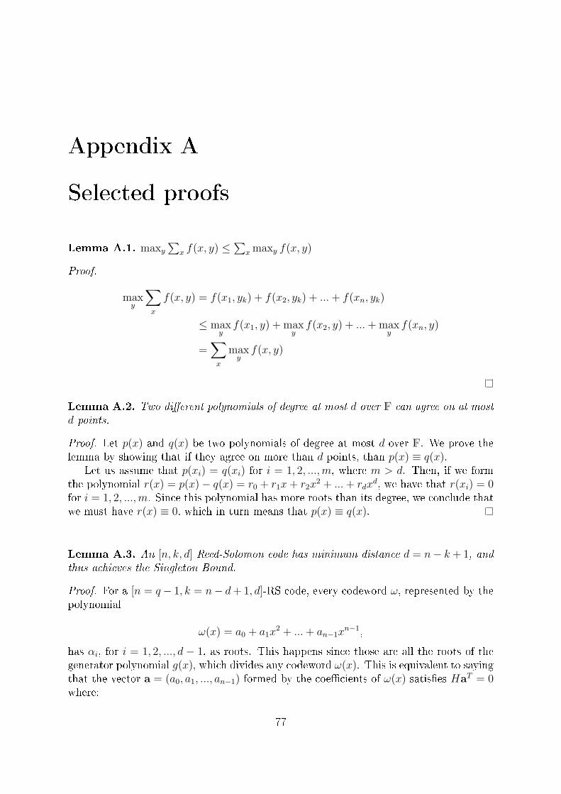
Appendix A
Selected proofs
Lemma A.1. maxy∑
x f(x, y) ≤∑
x maxy f(x, y)
Proof.
maxy
∑x
f(x, y) = f(x1, yk) + f(x2, yk) + ...+ f(xn, yk)
≤ maxyf(x1, y) + max
yf(x2, y) + ...+ max
yf(xn, y)
=∑x
maxyf(x, y)
Lemma A.2. Two di�erent polynomials of degree at most d over F can agree on at mostd points.
Proof. Let p(x) and q(x) be two polynomials of degree at most d over F. We prove thelemma by showing that if they agree on more than d points, than p(x) ≡ q(x).
Let us assume that p(xi) = q(xi) for i = 1, 2, ...,m, where m > d. Then, if we formthe polynomial r(x) = p(x)− q(x) = r0 + r1x+ r2x
2 + ...+ rdxd, we have that r(xi) = 0
for i = 1, 2, ...,m. Since this polynomial has more roots than its degree, we conclude thatwe must have r(x) ≡ 0, which in turn means that p(x) ≡ q(x).
Lemma A.3. An [n, k, d] Reed-Solomon code has minimum distance d = n− k + 1, andthus achieves the Singleton Bound.
Proof. For a [n = q− 1, k = n− d+ 1, d]-RS code, every codeword ω, represented by thepolynomial
ω(x) = a0 + a1x2 + ...+ an−1x
n−1,
has αi, for i = 1, 2, ..., d − 1, as roots. This happens since those are all the roots of thegenerator polynomial g(x), which divides any codeword ω(x). This is equivalent to sayingthat the vector a = (a0, a1, ..., an−1) formed by the coe�cients of ω(x) satis�es HaT = 0where:
77
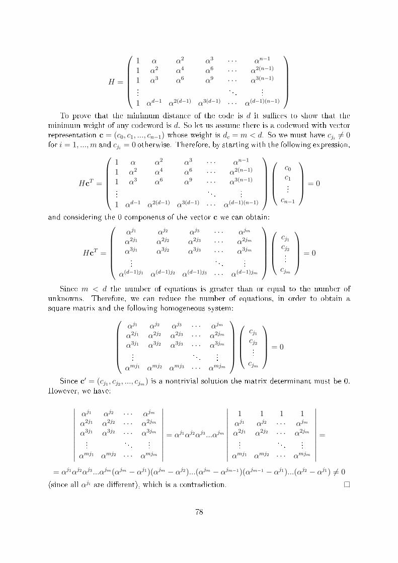
H =
1 α α2 α3 · · · αn−1
1 α2 α4 α6 · · · α2(n−1)
1 α3 α6 α9 · · · α3(n−1)
.... . .
...1 αd−1 α2(d−1) α3(d−1) · · · α(d−1)(n−1)
To prove that the minimum distance of the code is d it su�ces to show that the
minimum weight of any codeword is d. So let us assume there is a codeword with vectorrepresentation c = (c0, c1, ..., cn−1) whose weight is dc = m < d. So we must have cji 6= 0for i = 1, ...,m and cji = 0 otherwise. Therefore, by starting with the following expression,
HcT =
1 α α2 α3 · · · αn−1
1 α2 α4 α6 · · · α2(n−1)
1 α3 α6 α9 · · · α3(n−1)
.... . .
...1 αd−1 α2(d−1) α3(d−1) · · · α(d−1)(n−1)
c0c1...
cn−1
= 0
and considering the 0 components of the vector c we can obtain:
HcT =
αj1 αj2 αj3 · · · αjm
α2j1 α2j2 α2j3 · · · α2jm
α3j1 α3j2 α3j3 · · · α3jm
.... . .
...α(d−1)j1 α(d−1)j2 α(d−1)j3 · · · α(d−1)jm
cj1cj2...cjm
= 0
Since m < d the number of equations is greater than or equal to the number ofunknowns. Therefore, we can reduce the number of equations, in order to obtain asquare matrix and the following homogeneous system:
αj1 αj2 αj3 · · · αjm
α2j1 α2j2 α2j3 · · · α2jm
α3j1 α3j2 α3j3 · · · α3jm
.... . .
...αmj1 αmj2 αmj3 · · · αmjm
cj1cj2...cjm
= 0
Since c′ = (cj1 , cj2 , ..., cjm) is a nontrivial solution the matrix determinant must be 0.However, we have:
∣∣∣∣∣∣∣∣∣∣∣
αj1 αj2 · · · αjm
α2j1 α2j2 · · · α2jm
α3j1 α3j2 · · · α3jm
.... . .
...αmj1 αmj2 · · · αmjm
∣∣∣∣∣∣∣∣∣∣∣= αj1αj2αj3 ...αjm
∣∣∣∣∣∣∣∣∣∣∣
1 1 1 1αj1 αj2 · · · αjm
α2j1 α2j2 · · · α2jm
.... . .
...αmj1 αmj2 · · · αmjm
∣∣∣∣∣∣∣∣∣∣∣=
= αj1αj2αj3 ...αjm(αjm − αj1)(αjm − αj2)...(αjm − αjm−1)(αjm−1 − αj1)...(αj2 − αj1) 6= 0
(since all αji are di�erent), which is a contradiction.
78
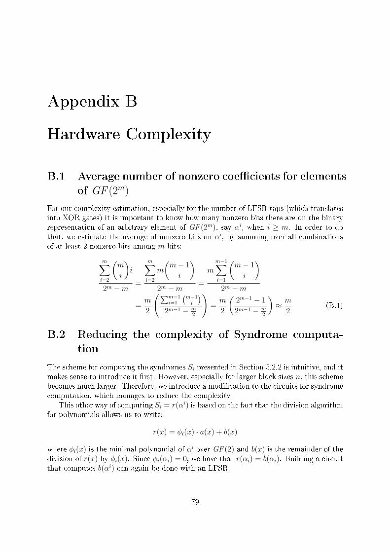
Appendix B
Hardware Complexity
B.1 Average number of nonzero coe�cients for elements
of GF (2m)
For our complexity estimation, especially for the number of LFSR taps (which translatesinto XOR gates) it is important to know how many nonzero bits there are on the binaryrepresentation of an arbitrary element of GF (2m), say αi, when i ≥ m. In order to dothat, we estimate the average of nonzero bits on αi, by summing over all combinationsof at least 2 nonzero bits among m bits:
m∑i=2
(m
i
)i
2m −m=
m∑i=2
m
(m− 1
i
)2m −m
=
mm−1∑i=1
(m− 1
i
)2m −m
=m
2
(∑m−1i=1
(m−1i
)2m−1 − m
2
)=m
2
(2m−1 − 1
2m−1 − m2
)≈ m
2(B.1)
B.2 Reducing the complexity of Syndrome computa-
tion
The scheme for computing the syndromes Si presented in Section 5.2.2 is intuitive, and itmakes sense to introduce it �rst. However, especially for larger block sizes n, this schemebecomes much larger. Therefore, we introduce a modi�cation to the circuits for syndromecomputation, which manages to reduce the complexity.
This other way of computing Si = r(αi) is based on the fact that the division algorithmfor polynomials allows us to write:
r(x) = φi(x) · a(x) + b(x)
where φi(x) is the minimal polynomial of αi over GF (2) and b(x) is the remainder of thedivision of r(x) by φi(x). Since φi(αi) = 0, we have that r(αi) = b(αi). Building a circuitthat computes b(αi) can again be done with an LFSR.
79
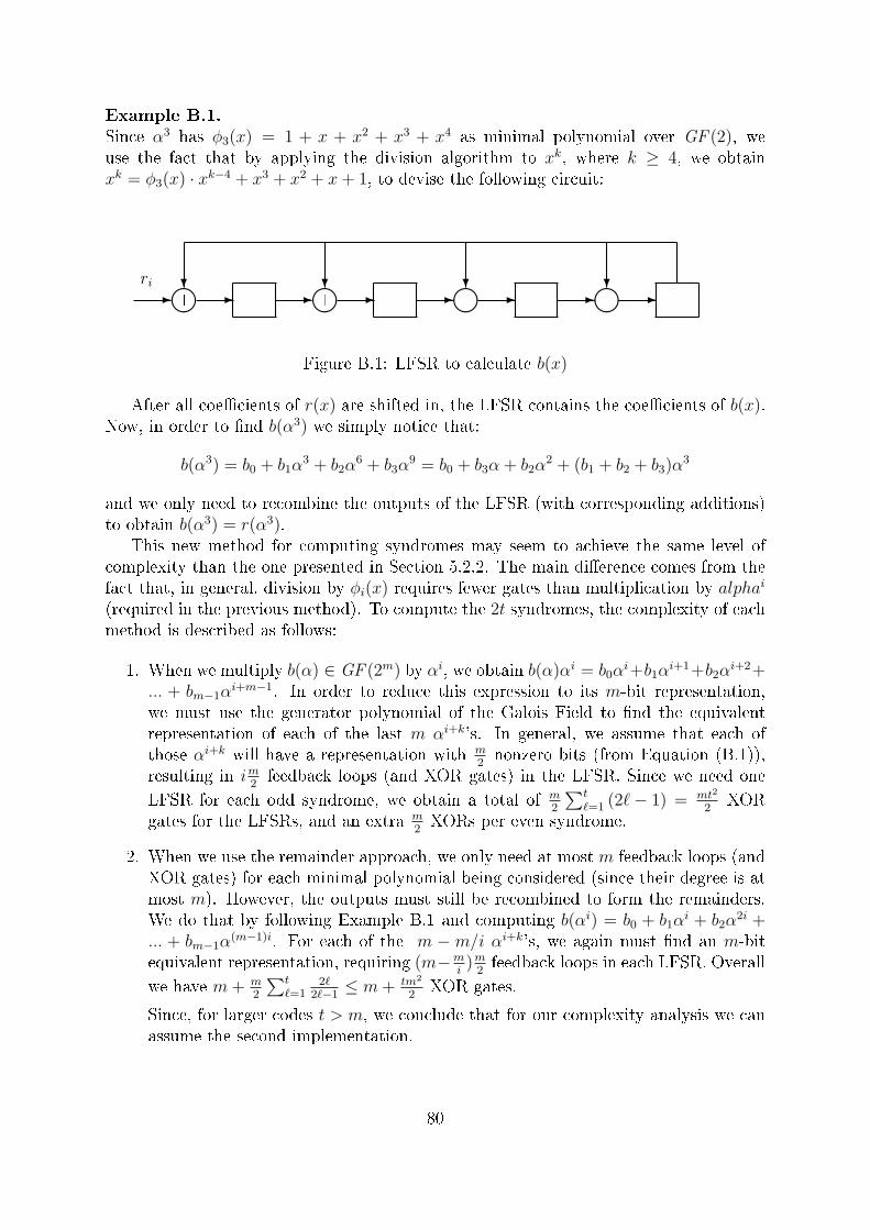
Example B.1.Since α3 has φ3(x) = 1 + x + x2 + x3 + x4 as minimal polynomial over GF (2), weuse the fact that by applying the division algorithm to xk, where k ≥ 4, we obtainxk = φ3(x) · xk−4 + x3 + x2 + x+ 1, to devise the following circuit:
- - - -� �� � �� � �� � ��- - - -+ + + +
? ? ? ?ri
Figure B.1: LFSR to calculate b(x)
After all coe�cients of r(x) are shifted in, the LFSR contains the coe�cients of b(x).Now, in order to �nd b(α3) we simply notice that:
b(α3) = b0 + b1α3 + b2α
6 + b3α9 = b0 + b3α + b2α
2 + (b1 + b2 + b3)α3
and we only need to recombine the outputs of the LFSR (with corresponding additions)to obtain b(α3) = r(α3).
This new method for computing syndromes may seem to achieve the same level ofcomplexity than the one presented in Section 5.2.2. The main di�erence comes from thefact that, in general, division by φi(x) requires fewer gates than multiplication by alphai
(required in the previous method). To compute the 2t syndromes, the complexity of eachmethod is described as follows:
1. When we multiply b(α) ∈ GF (2m) by αi, we obtain b(α)αi = b0αi+b1α
i+1+b2αi+2+
... + bm−1αi+m−1. In order to reduce this expression to its m-bit representation,
we must use the generator polynomial of the Galois Field to �nd the equivalentrepresentation of each of the last m αi+k's. In general, we assume that each ofthose αi+k will have a representation with m
2nonzero bits (from Equation (B.1)),
resulting in im2feedback loops (and XOR gates) in the LFSR. Since we need one
LFSR for each odd syndrome, we obtain a total of m2
∑t`=1 (2`− 1) = mt2
2XOR
gates for the LFSRs, and an extra m2XORs per even syndrome.
2. When we use the remainder approach, we only need at most m feedback loops (andXOR gates) for each minimal polynomial being considered (since their degree is atmost m). However, the outputs must still be recombined to form the remainders.We do that by following Example B.1 and computing b(αi) = b0 + b1α
i + b2α2i +
... + bm−1α(m−1)i. For each of the m − m/i αi+k's, we again must �nd an m-bit
equivalent representation, requiring (m−mi)m
2feedback loops in each LFSR. Overall
we have m+ m2
∑t`=1
2`2`−1≤ m+ tm2
2XOR gates.
Since, for larger codes t > m, we conclude that for our complexity analysis we canassume the second implementation.
80
B.3 Gate count for Inverter block
We can basically divide the inverter into three parts. For the "squarer" LFSR, we realizethat we will need m · m
2XORs. The array of AND gates essentially computes all m2 com-
binations between each bit from a and each bit from b. In order to estimate the numberof XORs needed for the combinational logic responsible for the parallel multiplication,we observe that when we multiply to generic elements of GF (2m), we obtain:(
a0 + a1α + a2α2 + ...+ am−1α
m−1) (b0 + b1α + b2α
2 + ...+ bm−1αm−1)
=
= a0b0 + (a0b1 + a1b0)α + ...+∑i+j=k
aibj αk + ...+ am−1bm−1α
2m (B.2)
Since all the pairs aibj are already available to us we just need to count the numberof sums, which, from Equation (B.2), turn out to be:
0 + 1 + 2 + ...+ (m− 2) + (m− 1) + (m− 2) + ...+ 2 + 1 + 0
However, the coe�cients of αi for i ≥ m actually become feedback loops (since wesimplify them to their m-bit representation). Since, according to Equation (B.1), weobtain in average m
2feedback loops for each such αi, we calculate the number of XORs
to be:
(0 + 1 + 2 + ...+ (m− 1)) +m
2((m− 2) + (m− 3) + ...+ 1 + 0) =
=m(m− 1)
2+m
2· (m− 1)(m− 2)
2=m3
4− m2
4(B.3)
B.4 Gate count for Chien's Search block
In the Chien's Search block, for each of the t blocks containing an αi multiplier, we havem �ip-�ops. Additionally, we obtain im
2LFSR taps, and we therefore have our total XOR
gates count to be:
m
2
2t∑i=1
i =m
2(2t+ 1) t =
m
2(2t+ 1) t = mt2 +
mt
2(B.4)
In the summation block, we need to take each of the m-bits from each of the t multiplierblocks, which requires a total of m(t− 1) XORs. To test whether the m bits of the resultare all 0 except for the least signi�cant one we need 2m NAND gates.
81
Appendix C
Sudan's algorithm maple source code
# Matthew Dailey and Ilan Shomorony
# advised by Prof. Martin
# March 3, 2009
# Sudan list decoding algorithm
with(linalg):
with(PolynomialTools):
with(difforms):
# input n,d,t set of points m,l
# need Q(x,y) to have weighted degree at most m+Ld
# This procedure implements Sudan's list decoding algorithm
# n is the number of points
# d is the maximum degree of a polynomial that one is searching for
# t is the number of points in which a polynomial found must match
the n points in
# m,L are used as parameters and are used for creating Qxy
# allPts is a list of the points stored in a [n x 2] array
# theModulus in a prime number representing which field we are
working over
sudanCoeff:=proc(n,d,t::integer,m,L,allPts, theModulus)
local numPoints, numCoeff,
r,c,allTerms,coeffMat,term,pointX,pointY,coeff, j ,k, theRank,
i,b,B,Qxy, allPoly, solNum, copyMat, allFactors, listFacts,
numFact, kk, currPoly, currInverse,
Thm5, claim4B,boundN,copyCoeff:
# tell if the algorithm gurantees to return a polynomial if one
exists
Thm5 := d* ceil(sqrt(2*(n+1))/d)-floor(d/2);
claim4B := m+l*d:
82
boundN := (m+1)*(l+1)+d*(l+1)*l/2:
printf("For claim 3, we need : %d > : %d :=n\n", boundN, n);
printf("For claim 4, we need t := : %d > : %d\n" , t,
claim4B);
printf("For Theorem 5, we need t:= %d > %d\n", t, Thm5);
allPoly:= []: # a list with all the possible curves
numPoints := n:
# get all terms which have weighted degree less than or equal to
m+Ld
allTerms := simplify(sum(sum( (y^k)*(x^j) ,
j=0..m+(L-k)*d),k=0..L));
#print(allTerms);
numCoeff := nops(allTerms);
printf("numPoints = %d number of coefficients =
%d\n",numPoints, numCoeff);
# generate coefficient matrix
coeffMat := matrix(numPoints, numCoeff):
# Fill the coefficient matrix with the corrent values for each
point
# meaning for each term (i.e. x^2*y) fill in the x value and y
value from the current point
for c from 1 by 1 to numCoeff do
term := op( c, allTerms):
for r from 1 by 1 to numPoints do
pointX := allPts[r,1]:
pointY := allPts[r,2]:
coeff := subs(x=pointX, y=pointY, term):
coeffMat[r,c] := coeff:
end do:
end do:
# To reduce the matrix to find our coefficients
# we need to create the solution vector which is the zero vector
b:=vector(numPoints ):
for i from 1 by 1 to numPoints do
b[i]:=0:
end do:
# We need to use the inert form to row reduce our matrix to stay
in
# our finite field
coeffMat := Gaussjord(coeffMat, 'thRank', 'theDet') mod
theModulus ;
83
# Now we wish to solve for the coefficients of the terms, such
as x^2 and xy
# The number of free variables is equal to
(numCoeff-theRank):=numSolutions
B:=linsolve(coeffMat,b,'theRank',mm );
printf("The rank of the coefficient matrix is %d\n", theRank);
# For each free variable, we will set it equal to one and get
numSolutions different possible solution
# and for each one we will look for factors that are linear in y.
for solNum from 1 by 1 to 1 do #(numCoeff-theRank) -- is
number of different free variables
copyMat:= evalm(B):
# Set the specific variable equal to one and all others zero
for i from 1 by 1 to (numCoeff - theRank) do
for j from 1 by 1 to numCoeff do
if i = solNum then
copyMat[j] := subs( mm[i]=1, copyMat[j]):
else
copyMat[j] := subs( mm[i]=0, copyMat[j]):
end if:
end do:
end do:
# Now we have a specific solution and we print it out
# we take the coefficients and dot product them with the
actual terms to construct the polynomial
Qxy:=sum( copyMat[ii]*op(ii, allTerms),ii=1..numCoeff) :
printf("Solution number %d, and polynomial\n ",solNum);
# now we want to loop through all the factors and find all
those which are linear in y
# and output their inverses (of f(x)) such that we write a
factor linear in y as (y-f(x))
allFactors := Factors(Qxy) mod theModulus:
print(allFactors);
# if we have non-trivial factors
if nops(allFactors) = 2 then
listFacts := allFactors[2]:
numFact := nops(listFacts):
for kk from 1 by 1 to numFact do
currPoly := (listFacts[kk])[1]: # get the actual factors
# printf("Current polynomial :: %a\n", currPoly);
84
# find the inverse, if it exits and add it to the list
currInverse := findInverse( currPoly, y, theModulus):
if currInverse <> -1 then
print(currInverse);
end if:
#-----------------------------------------------------------------
# make sure that for each of the polynomials that we will
return
# that it agrees in at least t places with the points we
inputted
if currInverse <> -1 and isMatcht( t, allPts, n,
currInverse, theModulus) then
allPoly := [op(allPoly), currInverse]:
end if:
end do:
end if:
end do:
# return all possible found polynomials in a list
return allPoly:
end proc:
# This procedure takes in a value t, a list of points, and an
expression in x, a modulus, the number of points
# it returns true if f(points_x_i_value) = (y_i mod theMod) for at
least t x_i's
# The points can have repeated x coordinates
# however, for our usage, the points should not have repeated
coordinates
isMatcht := proc( t::integer, allPts, numPts::integer,
anExpression, theMod::integer)
local numMatches, i:
numMatches := 0:
for i from 1 by 1 to numPts do
if allPts[i,2] = ( subs(x=allPts[i,1], anExpression) mod
theMod ) then
numMatches := numMatches + 1:
end if:
end do:
printf ("numMatches is %d and t is %d and degree is %d\n",
85
numMatches, t, degree(anExpression,x));
return numMatches >= t:
end proc:
# Procedure to build the terms for Sudan's algorithm
# this creates Qxy
generateAllTerm := proc(l::integer, m::integer, d::integer)
local allTheTerms:
allTheTerms := simplify(sum(sum(y^k*x^j, j = 0 .. m+(l-k)*d), k
= 0 .. l)):
return simplify(allTheTerms):
end proc:
# a procedure to make aPoly = (aVar - f(x)) and then find the
inverse of
# f(x) mod primeField
# Requires the coefficient of aVar is a constant
findInverse:=proc(aPoly, aVar, primeField)
local theCoeff, newPoly:
# Look through aPoly to see if it is linear in aVar
# if it is, then find aVar-newPoly := aVar (mod primeField)
# Then find the inverse of newPoly (mod primeField)
# return this value, or -1 if not found
if type(aPoly, linear(aVar)) = false then
return -1:
end if:
# extract the coefficient of aVar
theCoeff := coeff(aPoly,y,1):
# make sure the coefficient is a constant
if type(theCoeff, const) = false then
return -1:
end if:
newPoly := (-1*(aPoly - theCoeff*aVar)) mod primeField:
# if the factor is just c*y, then 0 does not have an inverse
(i.e. newPoly = 0 now)
if newPoly = 0 then
return -1:
end if:
86
newPoly := (newPoly / theCoeff) mod primeField:
newPoly := simplify(newPoly): # standard way to write
return newPoly;
end proc:
# this procedure will generate n random points with success
probability p
# of the function thePoly, and will generate a random field
element otherwise
# the field elements are from 0 to (theMod - 1)
# This function returns a list n by 2 matrix of the (x,thePoly(x))
points
# if a fifth argument is included, it is a list of points with the
x values entered.
genListPoints := proc(n::posint, thePolyB, theMod, p)
local numCorrPoints, thePoints, THEMAXRAND, theNoise,
noiseLevel, roll, i, aVal:
numCorrPoints := 0: # for our records, how many successful
points
# for randomness of the x values and for probability
THEMAXRAND := 1000000:
theNoise := rand(1..THEMAXRAND):
noiseLevel := ceil(p*THEMAXRAND): # if below this value, success
roll := rand(0 .. theMod-1):
# See if the user sent in the points
if nargs(args) = 4 then
thePoints := matrix(n, 2):
for i from 1 to n do
thePoints [i, 1] := roll();
end do:
else # user sent in the points
thePoints := args[5]:
end if:
# generate the (x,y) points
for i from 1 to n do
aVal := theNoise():
if p = 0 then
thePoints [i, 2] := roll():
87
elif aVal < noiseLevel then
# generate a real point
thePoints [i, 2] := thePolyB(thePoints[i, 1]) mod theMod;
numCorrPoints := numCorrPoints + 1:
else
# generate a random point
thePoints [i, 2] := roll():
if thePoints[i,2] = ( thePolyB(thePoints[i,1]) mod theMod)
then
numCorrPoints := numCorrPoints + 1:
end if:
end if:
end do:
printf("Number of actual points generated by %a is: %d\n",
thePoly, numCorrPoints);
return thePoints:
end proc:
# this procedure will generate n random unique x coordinates
# the field elements are from 0 to (theMod - 1)
# This function returns a list n by 2 matrix of the (x, - ) points
genListUniqueX:= proc(n::posint, theMod)
local THEMAXRAND,roll, i, aVal, allPossPts, thePts, tempPoint, j;
thePts := matrix(n, 2);
if n > theMod then
printf("Not enough field elements\n");
return:
end if:
# This will tell us if the point has been chosen already
allPossPts := matrix(theMod, 2):
for i from 1 to theMod do
allPossPts[i,1] := i mod theMod:
allPossPts[i,2] := 0: # not yet selected
end do:
roll := rand(1 .. theMod):
88
for i from 1 to n do
tempPoint := roll();
for j from 1 by 1 while allPossPts[tempPoint, 2] = 1 do
tempPoint := roll();
end do:
# now have a unique x coordinate, add it
allPossPts[tempPoint,2] := 1;
thePts[i,1] := tempPoint mod theMod:
end do:
return thePts:
end proc:
#*************************************************************
#*************************************************************
#*************************************************************
# NOW the new way to call the procedure
myN:= 16: # number of points to generate
theMod := 17: # We are working in Z mod theMod
# This is the probability of selecting a random point
p := .7: # the probability that the random point will be from the
function
f := x -> 4*x^3 + 9*x^2+3*x+2 mod theMod: # the polynomial we are
trying to find
d := 3; # the maximum degree of a polynomial we are looking for
n:= 16:
m:=ceil(d/2) - 1;
m:= 1:
l := ceil ( sqrt(2*(n+1)/d) ) - 1;
l:= 3:
# The number of places in which a factor must match the list of
points
t := max(m+l*d+1, d*(l+1)-m + 1):
# generate all the terms needed
allTerms := generateAllTerm(l, m, d):
# Create unique x points
theMat := genListUniqueX(myN, theMod):
89

# assign y values to these points
theMat := genListPoints(myN, f, theMod, p, theMat):
theMat := evalm(theMat):
# Call sudan's list decoding algorithm
A := sudanCoeff(myN, d, t, m, l, theMat, theMod):
90