Embed Size (px)
Citation preview

University of Tokyo Graduate School of Public Policy
Project Title: “Establishment of URS Campus in Jalajala, Rizal,
Philippines”
Economic Analysis of Public Policy Yoishitsugu Kanemoto
Alamo, Leah Azzani, Meikha
Veloso Camelo Pacheco, Jose Dinis Oyunsuren, Enkhchimeg
August, 2014

TABLE OF CONTENTS
EXECUTIVE SUMMARY .......................................................................................................... 3
1. INTRODUCTION..................................................................................................................... 5
1.1. Project Background .............................................................................................................. 5
1.2. Project Purposes ................................................................................................................... 5
1.3. Research Questions .............................................................................................................. 5
2. LITERATURES REVIEW AND THEORETICAL FRAMEWORK ........................................ 6
2.1. Literatures Review ............................................................................................................... 6
2.2. Theoretical Framework of Cost-Benefit Analysis (CBA) for Education Project ................ 8
2.3. Limitation of CBA for education project ........................................................................... 11
3. PRIMARY MARKET ANALYSIS ....................................................................................... 12
3.1. Primary Market .................................................................................................................. 12
3.1.1. Demand ........................................................................................................................ 12
3.1.2 Supply............................................................................................................................... 13
3.2. Cost and Benefit ................................................................................................................. 14
3.2.1. Costs ............................................................................................................................ 14
3.2.2. Benefits ........................................................................................................................ 17
3.3. Net Present Value (NPV) and Benefit-Cost Ratio (BCR).................................................. 21
4. SECONDARY MARKET ANALYSIS ................................................................................. 25
4.1. Supply- side Analysis .................................................................................................... 27
4.1.1. Accumulated data ........................................................................................................ 27
4.1.2. Findings ....................................................................................................................... 28
4.2. Demand- side Analysis ...................................................................................................... 28
4.3. Labor flows ........................................................................................................................ 30
4.4. Results ................................................................................................................................ 30
4.5. Sensitivity Analysis ............................................................................................................ 31
5. CONCLUSION ....................................................................................................................... 31

EXECUTIVE SUMMARY
As a developing country, Philippine has undergone major improvement on its economic
performance by improving its education system and attainment. Its rank in Human Development
Index in 2013 is 102. There is significant improvement of Philippine scores in HDI components,
especially in education. Philippine has focused to improve its education system since “a deep
regard” for education (DepEd 2008). Despite its improvement in education in country level,
there is significant decline of education standard in several provinces such as in Rizal. In Rizal
province, HDI decreased for 16.4% (HDN, 2013) because the score for education and income
indexes decreased for 2.8% and 31% consecutively in 2013
Focusing to municipality level, Jalajala as a part of Rizal province, encounters major issue in
education due to lack of affordable higher education institution. Every year 70% of the high
school graduates from Jalajala do not strive for higher education due to high cost. Many of
whom also do not have access to receive short term vocational education training, which should
assist them to be employed in the long-run. As a result, 33 percent of the current workforce in
Jalajala (TESDA, 2011) receive the salary of minimum wage as they have high school degree
and do not fully utilize their potential to earn more.
With the intention to promote literacy and education in the area, the Jalajala municipality is
introducing the development of the URS-LGU Jalajala skills training program. The initiative
provides youth, especially fresh high school graduates who struggle with the rising education
costs, with the opportunity to attend quality-driven and knowledge-rich college programs. The
higher education includes four years undergraduate program on five majors.
In order to forecast the impact of this program on the municipality and on the society as a whole,
the study will comprise a projection period of 8 years and construct quantitative/ qualitative
analysis on how much benefit this fully- government funded project can provide. The analysis
comprises the effect from the establishment of URS-LGU Jalajala in both primary and secondary
markets. To analyze whether the project is viable or not, the study incorporates Cost and Benefit
Analsysis (CBA) method. The alternative of the establishment of URS-LGU Jalajala is no

education or no new campus in Jalajala. Conclusion on whether the project will be continued or
not will be dependent from the result of CBA.
Primary market in this study is assumed to be “first best economy” with negligible price
distortion. Tuition and other school fees or the price approximate the marginal cost, thereby
supply curve is horizontal. As usually the case, demand curve is downward sloping. However,
due to data limitation and for conservatism, the analysis did not account for the resulting increase
in consumer surplus in the primary market.
The result of CBA calculation shows that taking into consideration the 15% social discount rate,
the Net Present Value (NPV) and Benefit-Cost Ratio (BCR)can be derived for this project. The
present value of total benefits is P234,401,148 and the present value of total costs is
P166,273,294. Therefore, the NPV is 68,127,854 and the CBR is 1.41. Based on both NPV and
BCR, it can be inferred that the benefits of the project greatly outweigh the costs.
As for secondary market, the analysis is based on labor market forecast model suggests that by
increasing supply, the average wage of university graduates will change; however, the wage
would not necessarily decrease as assumed. The change of wage is different across
occupation/sector specific. For technician/IT, by adding 49 graduates to the Rizal labor market
increase the average wage of university students by 1%. However, work accession rate and
separation rate are close. In other words, the possibility of getting hired is as same as getting
fired. International labor migration is decreasing over the years. In service sector, adding 99
graduates to the Rizal labor market increase the average wage of university students by 0.6%.
Work accession rate is higher than work separation rate.The labor demand market is increasing.
Getting hired is easier than being fired. However, international labor migration is considered to
be remaining still high. Lastly in business sector, adding 49 graduates to the Rizal labor market
decrease the average wage of university students by 0.1%. Work accession rate is higher than
work separation rate. The labor demand market is increasing. Getting hired is easier than being
fired. International labor migration is decreasing over the years.

1. INTRODUCTION
1.1. Project Background Jalajala is a fourth class municipality situated on the southern part of Rizal,covering waterfront
area to the largest freshwater lake, Laguna de Bay. Located 75km from the country capital, the
municipality is a home to 28,728 residents. Although agriculture, especially fish pen operating is
the main economic activity of Jalajala, opportunity from neighboring big metropolitan cities and
big towns of Rizal make it easier for people to find employment on other sectors.
According to Rizal local government, education attainment has become an issue of Jalajala due
to lack of affordable higher education institution. Every year 70% of the high school graduates
from Jalajala do not strive for higher education due to high cost. Many of whom also do not have
access to receive short term vocational education training, which should assist them to be
employed in the long-run. As a result, 33 percent of the current workforce in Jalajala (TESDA,
2011) receive the salary of minimum wage as they have high school degree and do not fully
utilize their potential to earn more.
1.2. Project Purposes With the intention to promote literacy and education in the area, the Jalajala municipality is
introducing government- subsidized URS-LGU Jalajala skills training program. The initiative
provides youth, especially fresh high school graduates who struggle with the rising education
costs, with the opportunity to attend quality-driven and knowledge-rich college. Students who
are attending can pay mere minimum to earn the undergraduate education. This being said, the
program’s goal is to nurture students with sets of skills, enabling their capacity to contribute for
the continuous thrive of the local economy through provision of low cost higher education. The
higher education includes four years undergraduate program on five majors, namely Business,
Technician/ IT, Social science and Teaching. The project has the capacity to prepare around 200
graduates each from from the abovementioned classes.
1.3. Research Questions In order to forecast the impact of this program on the municipality and on the society as a whole,
the study will comprise a projection period of 8 years and construct quantitative/ qualitative
analysis on how much benefit this government funded project can provide. The analysis

comprises the effect from the establishment of URS-LGU Jalajala in both primary and secondary
markets.
To analyze whether the project is viable or not, the study incorporates Cost and Benefit Analysis
(CBA) method. The alternative of the establishment of URS-LGU Jalajala is no education or no
new campus in Jalajala. Conclusion on whether the project will be continued or not will be fully
from the result of CBA. As for the study of secondary market, labor- market forecasting model
was used to understand 1) supply- side analysis, 2) demand- side analysis and 3) labor migration
flow.
2. LITERATURES REVIEW AND THEORETICAL FRAMEWORK
2.1. Literatures Review High economic growth is a major goal of economic activity in every country. From recent
economic growth theory, human capital is one of determinants of economic growth. Good
human capital allows a country to have higher productivity of output level which in turn high
economic growth. Therefore, spending in education policy becomes a concern in every country.
Education has been viewed as investment. Giving good education will raise not only wellbeing
of the people but also beneficial for an economy. Theoretically, education may affect economic
growth from three channels. First is from labor force productivity. Education improves the
quality and productivity of human capital which enable to economy to move to higher level of
output. Second, education promotes innovation, new technology and knowledge that boost
economic growth. Lastly, education is also believed to be able to serve as transmitter and
catalisator to comprehend and implement new technology and information which eventually
boost economic growth.
Hanushek (2010) finds the association of education and economic growth by simply plotting
years of education and economic growth. Figure 1 shows association between years of education
and economic growth. Representation of the association is that years of education are associated
with long-run growth that is 0.58 percentage points higher. However, each country has different
system and even quality of education. Putting solely the measurement of education in years of
education is arguably. Therefore, considering the impact of quality of education is necessary.
Study from Barro (2001) confirms the impact of the quality of education to economic growth.

From macroeconomic point of view, education, measured either by time or quality, affects
economic growth.
Figure 1: The Association of Years of Education and Economic
Source: Hanushek, 2010
Meanwhile from household’s point of view, having higher education is highly related to higher
income. It has been viewed that the benefit of adding one more year of education may increase
income since it is associated to higher skill and productivity. Studies that find the relationship of
education and income
In regard to Philippine, the country’s economic development is considered as developing
countries. Its rank in Human Development Index in 2013 is 102. There is significant
improvement of Philippine scores in HDI components, especially in education. Philippine has
focused to improve its education system since “a deep regard” for education (DepEd 2008).
Figure 2 shows the association of HDI and per capita income. As HDI increases, it is likely that
per capita income also increases.
In particular to Rizal province that has experienced declining of income, its HDI has decreased
as well for 16.4% (HDN, 2013). In Rizal province, the score for education and income indexes
decreases for 2.8% and 31% consecutively.
Figure 2: The Relationship of Education and Per Capita Income
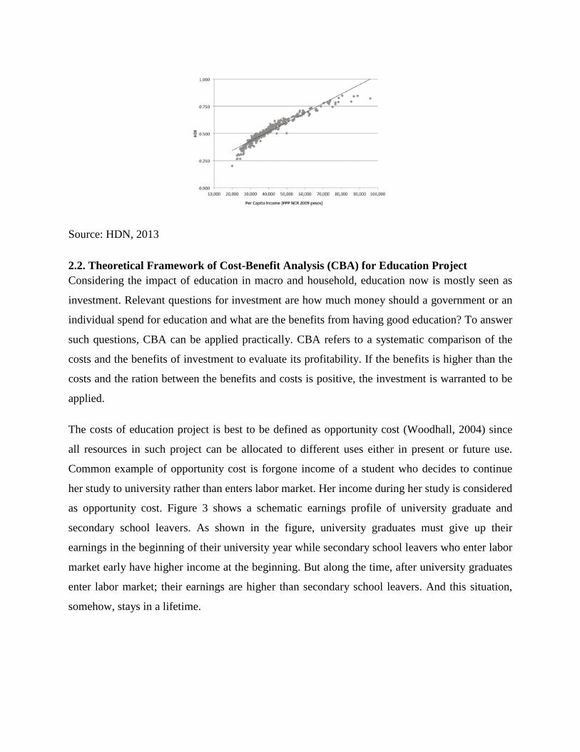
Source: HDN, 2013
2.2. Theoretical Framework of Cost-Benefit Analysis (CBA) for Education Project Considering the impact of education in macro and household, education now is mostly seen as
investment. Relevant questions for investment are how much money should a government or an
individual spend for education and what are the benefits from having good education? To answer
such questions, CBA can be applied practically. CBA refers to a systematic comparison of the
costs and the benefits of investment to evaluate its profitability. If the benefits is higher than the
costs and the ration between the benefits and costs is positive, the investment is warranted to be
applied.
The costs of education project is best to be defined as opportunity cost (Woodhall, 2004) since
all resources in such project can be allocated to different uses either in present or future use.
Common example of opportunity cost is forgone income of a student who decides to continue
her study to university rather than enters labor market. Her income during her study is considered
as opportunity cost. Figure 3 shows a schematic earnings profile of university graduate and
secondary school leavers. As shown in the figure, university graduates must give up their
earnings in the beginning of their university year while secondary school leavers who enter labor
market early have higher income at the beginning. But along the time, after university graduates
enter labor market; their earnings are higher than secondary school leavers. And this situation,
somehow, stays in a lifetime.

Figure 3: Stylized Age-Earnings Profile
Source: Jimenez and Patrinos (2008)
Other concept of costs for education project is social cost. This includes salary of teachers, study
materials, and other related goods and services that are supplied by public fund. Those
expenditures can also be private costs if an individual should provide them by their selves.
Widhall (2004) resumes social and private costs of education in Table 1.
Table 1: Costs of Education
Social cost Private cost
Direct
Teacher salaries Fees, minus average value of scholarships
Other current expenditure pn goods and services Books, etc
Expenditure on books
Imputed rent
Indirect
Earnings forgone Earnings forgone
Source: Windhal, 2004.
Measurement of the benefits is from lifetime earnings of educated people compared to non-
educated people, in other words this is social return (see Figure 3). However, calculating the

benefit of education from lifetime income is not sufficient. Education has huge effect or indirect
effect to society which is difficult to monetize. Such benefit usually refers as positive
externalities that may come in many forms. One of examples of positive externalities is the
declining of fertility rate as more women go to school rather than marry in young age.
There are two approaches to valuing the benefits of education that are national income and
consumer surplus approaches. Most often, consumer surplus approach is used to valuing the
benefits. Consumer surplus approach measures changes in consumer and producer surpluses in a
market directly affected by a policy. It must be considered whether the market is with or without
price distortion (first best economy). In a first best economy where market is efficient but price
effect is negligible, supply curve is horizontal and is marginal cost (price), while demand curve
has downward sloping. In this kind of market, the movement of demand curve does not change
the price but only quantity as shown by Figure 4. Existing consumers in this market are not
influenced In contrast, in an efficient market with price effect, change in demand curve will
definitely change price. Existing consumers in this market is influenced by the policy.
Figure 5: Primary Market in Best Economy with and without Price Effect
Primary Market in Best Economy without Price Effect
Primary Market in Best Economy with Price Effect

Change in primary market may bring indirect effect to secondary market due to policy
implementation. Figure 6 illustrates how change in primary market has an effect to other market
as well.
Figure 6: Primary and Secondary Markets
Formula to calculate the costs and the benefits are in the following (equation 1). Both the costs
and the benefits must be discounted to their present value. The private benefit (B) of having
more years of education is the earning that last for the rest of a person’s life while the private
cost (C) is any cost incurred due to having more years of education plus opportunity cost due to
forgone income. Investment will be continued as long as the net present value is positive.
∑𝐵𝑡/(1 + 𝑟)𝑡 = ∑𝐶𝑡/(1 + 𝑟)𝑡 (1)
2.3. Limitation of CBA for education project Despite its practical implementation for education project, CBA has some limitations (Jimenez
and Patrinos, 2008). Firstly, when estimating social returns, alternatives used are often assumed
to be no education. It is because traditionally, CBA for education project assumes that
government is the only financial source. Thus, the alternatives are when government does not
provide education while actually there are many alternatives such as letting private sector to
provide education. According to Jimenez and Patrinos (2008), this assumption leads to
overestimate of social returns.
Second limitation is its inability to include externality or non-market effects when estimating the
benefits of education. It is because externalities are difficult to be monetized and it is often in
CBA calculation, externalities are neglected. For instance, the effect of education in improving

social equity in a country or reducing crime rate in society is problematic to be calculated or
monetized.
Estimating distributional objectives is the third limitation. Income redistribution and poverty
reduction are considered as social benefits. However, to calculate redistribution objective in a
standard CBA is difficult in practice although the method has been developed by using rate of
return formula.
Fourth limitation is correcting for market failure. So far income gap between university
graduates and secondary school leavers is considered as the benefits of education. This benefit is
actually arguably and may be overestimate the benefits of education. It is because skill and
productivity do not necessarily resulted by being longer at school but also experience. Jimenez
and Patrinos (2008) suggest that added productivity considered by labor market is because labor
market takes the sorting done by school.
Lastly, CBA cannot capture different effect of education project. Currently, education does not
only aim to expand the length of education but also quality of education. As many countries are
already succeeded to expand years of education, they tend to focus on the quality of education.
CBA cannot estimate the quality of education. Woodhall (2004) suggests to use cost
effectiveness analysis in the area where CBA cannot cover.
3. PRIMARY MARKET ANALYSIS
3.1. Primary Market In this project, the primary market dealt with the demand and supply for tertiary education. Due
to the limited access on data, we relied on the figures provided in the project proposal made by
the Municipality of Jalajala and other studies conducted in the Philippines relative to tertiary
education.
3.1.1. Demand The total demand pertains to the highschool graduates of Jalajala. In the past years, based on the
project proposal of Municipality of Jalajala, about 30% of them were able to enter various
universities. However, the proposal does not include the list of universities and the amount of
fees charged by those institutions to these students. Also, we cannot find reliable study

conducted regarding the varying amount of fees charged by the different universities/colleges in
the locality or in the Philippines. Hence, to find the number of enrollees, we relied on the
projection made by Municipality which is constrained by the capacity of the facilities. As in any
case, we can assume that demand curve is downward sloping.
3.1.2 Supply In the Philippines, educational institution is usually established as a non-profit organization and
shall not declare any dividend as such but shall use their resources for furtherance of its
operation as laid down in the Corporation Code. Further, schools are exempted from income tax.
Hence, we can say that tuition and other school fees or the price approximate the marginal cost,
supply curve is horizontal and there is no price distortion as in the case of “first best economy”.
Based on the data on tuition fee increase for school year 2012-2013, the average proposed tuition
per unit for Region IVA, the region where Rizal Province belongs, is P714.62. Based on the
proposal of the establishment the University of Rizal, Jalajala Campus shall charge P100 per unit
lower than the average school fees. This is within the range of fees charge in other campus of
the University of Rizal.
Given the explanation above and as discussed in the background study, primary market can be
depicted by this figure:
Figure 7: Primary Market
In this figure, P0 is the average price of school fees without the project and P1 is the price
charged by the University of Rizal, Jalajala Campus. Based on this illustration, there is an
additional consumer surplus in pursuing the project represented by the area “B”. However, since
reliable demand curve can hardly be established and for conservatism, the group decided not to
P1
P0 A
B

consider this additional consumer surplus in the computation of the cost and benefit of the
project.
3.2. Cost and Benefit
3.2.1. Costs The costs of the project include the fixed and variable (operating costs) costs, and opportunity
cost for students which are the amount of money they could earn had they not entered the
university.
3.2.1.1 Fixed Costs Fixed costs comprise of the cost of the land, building, and furniture and pieces of equipment that
will be used by this Campus. The building has a useful life of 20 years while furniture and
equipment have a useful life of 5 years. Since this project will run for 8 years, additional
furniture and equipment will be purchased on the 6th year. We use the estimated initial costs of
these fixed assets and adjust their prices based on average inflation to project their costs on the
6th year.
Table 2: Fixed Costs
Fixed Costs units price 1st Year 6th Year*
Furniture and Equipment
Armchair 1100 925.00 1,017,500.00 1,225,496.22
Computer Units 54 5,000.00 1,350,000.00 1,625,965.51
Teachers Table 17 2,500.00 42,500.00 51,187.80
Executive Chair 4 5,500.00 22,000.00 26,497.22
Executive Table 4 7,800.00 31,200.00 37,577.87
Monobloc Chairs 900 275.00 247,500.00 298,093.68
Modular Computer Table 54 1,500.00 81,000.00 97,557.93
Computer Chair 54 1,000.00 54,000.00 65,038.62
6 - 8 seater table 24 10,000.00 240,000.00 289,060.53
Multi Media Projector 3 35,000.00 105,000.00 126,463.98

Projector Screen 3 5,000.00 15,000.00 18,066.28
Aircon Units - 2hp 6 33,000.00 198,000.00 238,474.94
Aircon Units - 1hp 6 15,000.00 90,000.00 108,397.70
Science Lab Table 12 10,000.00 120,000.00 144,530.27
Cubicle/Divider 6 21,244.00 127,464.00 153,520.05
Book Shelves 15 10,000.00 150,000.00 180,662.83
Laboratory Cabinet 3 15,000.00 45,000.00 54,198.85
Microscope 3 50,000.00 150,000.00 180,662.83
Photo Copier 3 60,000.00 180,000.00 216,795.40
Scanner 3 5,000.00 15,000.00 18,066.28
Printer 3 8,000.00 24,000.00 28,906.05
Conference Table 1 15,000.00 15,000.00 18,066.28
Conference Chair 10 1,500.00 15,000.00 18,066.28
Fax Machine 1 9,000.00 9,000.00 10,839.77
Library Holdings 3 50,000.00 150,000.00 180,662.83
Welding Machine 9 15,000.00 135,000.00 162,596.55
Welding Mask 9 2,000.00 18,000.00 21,679.54
Filing Cabinet 9 10,000.00 90,000.00 108,397.70
Sub-total 4,737,164.00 5,705,529.83
Land 5,400,000.00
Building 30,200,000.00
TOTAL FIXED COSTS 10,137,164.00 5,705,529.83
* Average inflation rate of 3.79% from 2008 to 2013 was used to project the cost.
3.2.1.2 Variable Costs Variable costs include salaries of staff and faculty and utilities. We assume that salary will
increase every two years using the salary matrix used for government employees. Further, there

will be additional professors on 2nd to 4th year of operation. Other benefits comprise of
premium for social insurance system, health insurance, housing fund, mandatory allowances,
13th month pay and cash gifts. Utilities include electricity, water and communication costs. We
allocate P66.00 monthly for every student on the first year as suggested in the project proposal
and use the inflation rate to adjust costs for the succeeding years.
Table 3: Variable Costs
1st Year 2nd Year 3rd Year 4th Year 5th Year 6th Year 7th Year 8th Year
Basic 2,938,860.00 3,560,040.00 4,401,624.00 5,069,388.00 5,352,888.00 5,449,548.00 5,754,384.00 5,858,316.00
Other benefits 1,190,145.40 1,423,075.60 1,705,229.36 1,948,563.32 2,011,878.32 2,033,465.72 2,101,545.76 2,124,757.24
Sub-total 4,129,005.40 4,983,115.60 6,106,853.36 7,017,951.32 7,364,766.32 7,483,013.72 7,855,929.76 7,983,073.24
Utilities 274,032.00 526,090.75 695,376.00 863,280.00 860,904.00 858,528.00 862,488.00 861,696.00
Variable Cost 4,403,037.40 5,509,206.35 6,802,229.36 7,881,231.32 8,225,670.32 8,341,541.72 8,718,417.76 8,844,769.24
3.2.1.3 Opportunity Cost Opportunity cost pertain to amount of money students can earn for four years had they not
entered the university. We use the average daily rate for a highschool graduate determined in the
study conducted by Luo and Terada on Education and Wage Differentials in the Philippines
(using Year 2000 as base year) and adjust it using the average salary increase of 1.8% from 2008
to 2013. Recognizing that not all of them would be employed, we consider the unemployment
rate (49%) for the age group, 15-24, published in the Philippine Statistics Authority website.
Adjusted average daily rate2014 = P176.47 x (1 + 1.8%)(2014-2000) = P176.47 x (1 + 1.8%)14 =
P266.54
Adjusted annual salary2014 = P266.54 x 12 x 299 working days = P67,734.66

Table 4: Opportunity Costs
Year of Operation Factor Amount
No. of Students
Employment Rate Total Amount
a =
(1+1.8%)t-1 B C D e = a x b x c x d
1 1.00 67,734.66 213 51% 7,358,016.30
2 1.02 68,953.89 640 51% 22,506,548.26
3 1.04 70,195.06 878 51% 31,431,941.97
4 1.05 71,458.57 1090 51% 39,723,817.14
5 1.07 72,744.82 1087 51% 40,327,546.27
6 1.09 74,054.23 743 51% 28,061,368.43
7 1.11 75,387.20 458 51% 17,608,943.02
8 1.13 76,744.17 210 51% 8,219,300.96
3.2.2. Benefits Benefits from the project can be traced from the increase in salary of the graduates, revenue
from tuition and other fees and residual value of fixed assets including land
3.2.2.1 Increase in Salary of the Graduates The benefits that will be obtained from establishing the campus in Jalajala, Rizal will come
mainly from the difference between the income a college graduate can earn as against the income
a highschool graduate can make in their productive years. Again, we use the average daily rate,
for both degree holder (P354.86) and highschool (P176.47), determined in the study conducted
by Luo and Terada on Education and Wage Differentials in the Philippines (using Year 2000 as
base year) to compute for the marginal salary. We adjust it for succeeding years using the
average salary increase of 1.8% from 2008 to 2013. Further, we consider the unemployment rate
in the every age bracket (Table5) as published in the Philippine Statistics Authority website and
assume that the rest will be employed.

Table 5: Age Group and Unemployment Rate
AGE GROUP Unemployment Rate
15 – 24 49.00
25 – 34 30.75
35 – 44 10.10
45 – 54 6.35
55 – 64 3.15
65 and over 0.65
Marginal average daily rate2014 = (P 354.86 - P176.47) x (1 + 1.8%)(2014-2000) = P178.39 x (1 +
1.8%)14 = P229.14
Marginal annual salary2014 = P229.14 x 12 x 299 working days = P68,512.49
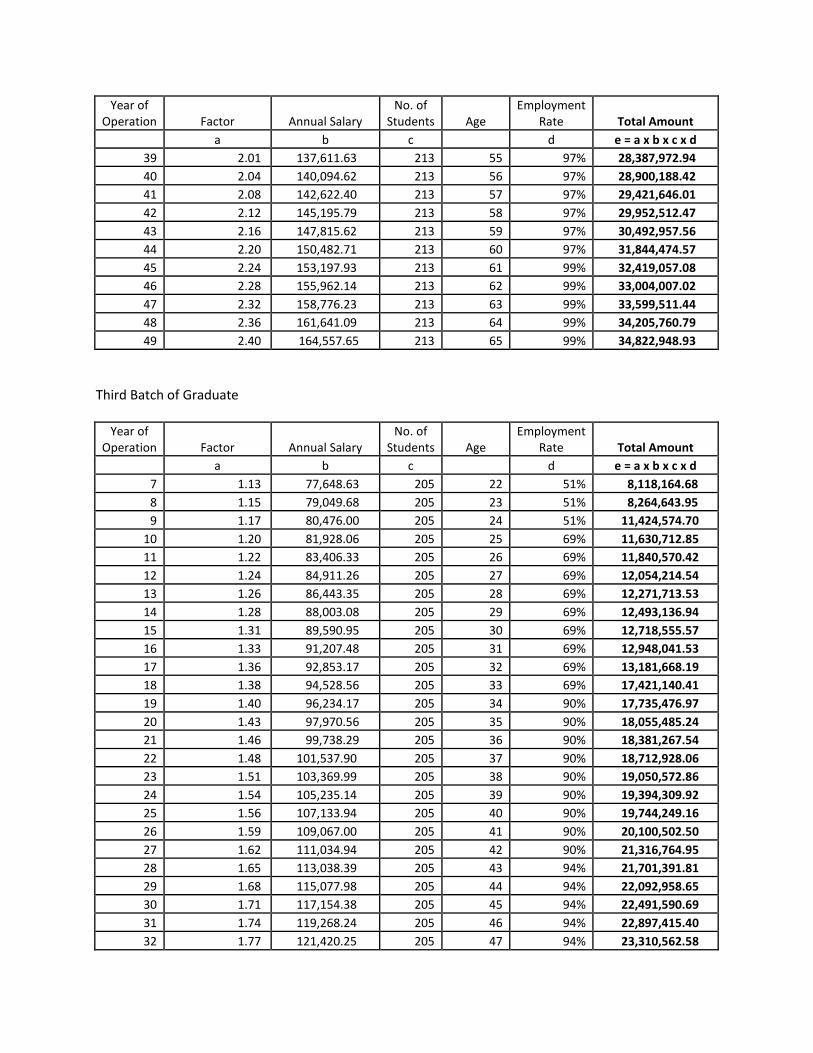
To illustrate, computation for the first batch of graduate is shown below. Computation other
batches is shown in Appendix ______.
Table 6: Illustration of Annual Salary of First Graduates
Year of Operation Factor Annual Salary No. of
Students Age Employment Rate Total Amount
A B C D e = a x b x c x d
5 1.09 74,920.60 213 22 51% 8,138,624.58
6 1.11 76,272.42 213 23 51% 8,285,473.02
7 1.13 77,648.63 213 24 51% 8,434,971.10
8 1.15 79,049.68 213 25 69% 11,660,025.29
9 1.17 80,476.00 213 26 69% 11,870,411.76
10 1.20 81,928.06 213 27 69% 12,084,594.32
11 1.22 83,406.33 213 28 69% 12,302,641.46
12 1.24 84,911.26 213 29 69% 12,524,622.92
13 1.26 86,443.35 213 30 69% 12,750,609.67

14 1.28 88,003.08 213 31 69% 12,980,673.99
15 1.31 89,590.95 213 32 69% 13,214,889.45
16 1.33 91,207.48 213 33 69% 13,453,330.95
17 1.36 92,853.17 213 34 90% 17,780,175.02
18 1.38 94,528.56 213 35 90% 18,100,989.79
19 1.40 96,234.17 213 36 90% 18,427,593.15
20 1.43 97,970.56 213 37 90% 18,760,089.54
21 1.46 99,738.29 213 38 90% 19,098,585.29
22 1.48 101,537.90 213 39 90% 19,443,188.66
23 1.51 103,369.99 213 40 90% 19,794,009.85
24 1.54 105,235.14 213 41 90% 20,151,161.04
25 1.56 107,133.94 213 42 90% 20,514,756.45
26 1.59 109,067.00 213 43 94% 21,756,085.01
27 1.62 111,034.94 213 44 94% 22,148,638.70
28 1.65 113,038.39 213 45 94% 22,548,275.39
29 1.68 115,077.98 213 46 94% 22,955,122.89
30 1.71 117,154.38 213 47 94% 23,369,311.30
31 1.74 119,268.24 213 48 94% 23,790,973.08
32 1.77 121,420.25 213 49 94% 24,220,243.07
33 1.80 123,611.08 213 50 94% 24,657,258.54
34 1.84 125,841.44 213 51 94% 25,102,159.26
35 1.87 128,112.05 213 52 97% 26,428,299.25
36 1.90 130,423.63 213 53 97% 26,905,155.56
37 1.94 132,776.91 213 54 97% 27,390,615.98
38 1.97 135,172.66 213 55 97% 27,884,835.76
39 2.01 137,611.63 213 56 97% 28,387,972.94
40 2.04 140,094.62 213 57 97% 28,900,188.42
41 2.08 142,622.40 213 58 97% 29,421,646.01
42 2.12 145,195.79 213 59 97% 29,952,512.47

43 2.16 147,815.62 213 60 97% 30,492,957.56
44 2.20 150,482.71 213 61 99% 31,844,474.57
45 2.24 153,197.93 213 62 99% 32,419,057.08
46 2.28 155,962.14 213 63 99% 33,004,007.02
47 2.32 158,776.23 213 64 99% 33,599,511.44
48 2.36 161,641.09 213 65 99% 34,205,760.79
3.2.2.2 Revenue from Tuition and Other Fees Revenue from tuition and other fees to be charged by URS-Jalajala Campus as a benefit as this
will diminish the costs that will be incurred by the government. Moreover, this an additional
benefit since such transaction would not be realized if this Campus will not be established. We
use the proposed tuition and other fees which is within the range of fees charged by other
campuses and adjust them using average inflation rate for the succeeding years
Table 7: Revenues
Year 1 Year 2 Year 3 Year 4 Year 5 Year 6 Year 7 Year 8
Enrollees 1st Yr.
346 346 334 343 341 341 341 341
2nd Yr. 294 294 284 292 290 290 290
3rd Yr. 250 250 241 248 247 247
4th Yr. 213 213 205 211 210
Total 346 640 878 1090 1087 1084 1089 1088
Fees Tuition Fee
2,400.00 2,490.96 2,585.37 2,683.35 2,785.05 2,890.61 3,000.16 3,113.87
Miscellaneous 1,660.00 1,722.91 1,788.21 1,855.99 1,926.33 1,999.34 2,075.11 2,153.76
Total 4,060.00 4,213.87 4,373.58 4,539.34 4,711.38 4,889.94 5,075.27 5,267.62
Semesters 2 2 2 2 2 2 2 2
Revenue 809,520.00 393,758.72 680,006.17 895,757.93 0,242,538.88 0,601,391.46 1,053,936.89 1,462,345.85

3.2.2.3 Horizon Value of Fixed Assets and Land Since we limit this study for 5 batches of graduates, we will account the amount that can be
allocated for the rest of the useful life of the fixed assets after the 8th year as residual value of
these assets. On the other hand, since land does not depreciate and usually appreciates, we use
its whole cost and inflation to project for the amount it will be saleable after the 8th year.
Table 8: Depreciable Assets
a. Depreciable Assets Furniture and Equipment* Building
Cost 5,705,529.83 30,200,000.00
Divided by useful Life 5 20
1,141,105.97 1,510,000.00
Multiplied by remaining useful life after 8th year 2 12
Residual Value 2,282,211.94 18,120,000.00
*purchased on 6th year b. Non-depreciable Asset
Value of Land2022 = P5,400,000.00 x (1+3.79%)(2022-2014) = P7,006,196.98 c. Total Horizon Value
Horizon Value = 2,282,211.94 + 18,120,000.00 +7,006,196.98 =27,408,408.91
3.3. Net Present Value (NPV) and Benefit-Cost Ratio (BCR)
The table below summarizes the benefits and costs. Amounts were discounted at 15%, the rate
used by the National Economic Development Authority (NEDA), the planning agency of the
Philippines.

Table 9: Benefits and Costs Calculation
Yr. Factor
Increase in Salary Revenue
Horizon Value
Total Benefits
Discounted Benefits
Fixed Cost
Variable Cost
Opportunity Cost
Total Costs
Discounted
Cost
1 1.0000
2,809,520
2,809,520 2,809,520 24,137,16
4 4,403,03
7 7,358,016 35,898,21
8 35,898,21
8
2 0.7561
5,393,759
5,393,759 4,078,456
5,509,206 22,506,548
28,015,755
21,183,935
3 0.6575
7,680,006
7,680,006 5,049,729
6,802,229 31,431,942
38,234,171
25,139,588
4 0.5718
9,895,758
9,895,758 5,657,932
7,881,231 39,723,817
47,605,048
27,218,341
5 0.4972 8,138,625 10,242,53
9
18,381,163 9,138,687
8,225,670 40,327,546
48,553,217
24,139,530
6 0.4323 16,570,946 10,601,39
1
27,172,337 11,747,351 3,423,318 8,341,54
2 28,061,368 39,826,22
8 17,217,97
7
7 0.3759 24,988,107 11,053,93
7
36,042,044 13,549,539
8,718,418 17,608,943
26,327,361 9,897,430
8 0.3269 37,018,372 11,462,34
6 27,408,409 75,889,127 24,808,290
8,844,769 8,219,301
17,064,070 5,578,275
9 0.2843 52,444,401
52,444,401 14,907,972 10 0.2472 59,685,414
59,685,414 14,753,322
11 0.2149 60,762,342
60,762,342 13,060,454 12 0.1869 61,858,701
61,858,701 11,561,834
13 0.1625 62,974,842
62,974,842 10,235,172 14 0.1413 64,111,122
64,111,122 9,060,739
15 0.1229 65,267,905
65,267,905 8,021,066 16 0.1069 66,445,559
66,445,559 7,100,689
17 0.0929 71,728,563
71,728,563 6,665,440 18 0.0808 81,182,212
81,182,212 6,559,938
19 0.0703 91,013,277
91,013,277 6,395,077 20 0.0611 92,655,466
92,655,466 5,661,275
21 0.0531 94,327,285
94,327,285 5,011,673

Yr. Factor
Increase in Salary Revenue
Horizon Value
Total Benefits
Discounted Benefits
Fixed Cost
Variable Cost
Opportunity Cost
Total Costs
Discounted
Cost
22 0.0462 96,029,270
96,029,270 4,436,609 23 0.0402 97,761,964
97,761,964 3,927,531
24 0.0349 99,525,922
99,525,922 3,476,867
25 0.0304 101,321,70
8
101,321,708 3,077,914
26 0.0264 104,021,06
8
104,021,068 2,747,752
27 0.0230 107,638,43
5
107,638,435 2,472,440
28 0.0200 111,365,19
1
111,365,191 2,224,385
29 0.0174 113,374,59
8
113,374,598 1,969,148
30 0.0151 115,420,26
1
115,420,261 1,743,198
31 0.0131 117,502,83
4
117,502,834 1,543,175
32 0.0114 119,622,98
5
119,622,985 1,366,104
33 0.0099 121,781,39
0
121,781,390 1,209,351
34 0.0086 123,978,74
0
123,978,740 1,070,584
35 0.0075 127,088,94
9
127,088,949 954,297
36 0.0065 131,126,61
2
131,126,612 856,187
37 0.0057 135,281,35
2
135,281,352 768,100
38 0.0049 137,722,28
7
137,722,287 679,965
39 0.0043 140,207,26
5
140,207,265 601,942
40 0.0037 142,737,08
1
142,737,081 532,872
41 0.0032 145,312,54
3
145,312,543 471,728

Yr. Factor
Increase in Salary Revenue
Horizon Value
Total Benefits
Discounted Benefits
Fixed Cost
Variable Cost
Opportunity Cost
Total Costs
Discounted
Cost
42 0.0028 147,934,47
5
147,934,475 417,600
43 0.0025 150,603,71
5
150,603,715 369,682
44 0.0021 154,122,43
8
154,122,438 328,973
45 0.0019 158,504,24
9
158,504,249 294,197
46 0.0016 163,005,70
6
163,005,706 263,089
47 0.0014 165,946,88
3
165,946,883 232,901
48 0.0012 168,941,12
8
168,941,128 206,176
49 0.0011 137,166,45
1
137,166,451 145,564
50 0.0009 104,190,12
7
104,190,127 96,147 51 0.0008 71,334,664
71,334,664 57,241
52 0.0007 36,224,643
36,224,643 25,276
Total
4,954,515,738
234,401,148
281,524,068
166,273,294
Net Present Value = PV of Benefit – PV of Cost = P234,401,148 - P166,273,294 = P68,127,854
Benefit-Cost Ratio = PV of Benefit/ PV of Cost = P234,401,148/P166,273,294 = 1.41
Taking into consideration the 15% social discount rate, the Net Present Value (NPV) and Benefit-Cost Ratio (BCR)can be derived for
this project. The present value of total benefits is P234,401,148 and the present value of total costs is P166,273,294. Therefore, the
NPV is 68,127,854 and the CBR is 1.41. Based on both NPV and BCR, it can be inferred that the benefits of the project greatly
outweigh the costs.

4. SECONDARY MARKET ANALYSIS
Figure 8: Basic Information of Rizal
• The population of Rizal is 1,476,572
• More than 85% of the residents have been living in the area for the last 5 years.
• Consists with 9 urban municipalities and four rural area- 1 secondary metropolitan city, 4 medium city, 2 large towns and 2 small towns
• As only 4.5% of the population lives in the rural area, non-agricultural sectors lead in this region.
Source: Rizal Provincial Government (2013) This part of the paper reviews what is known about the role of education in improving the labor
market outcome, with a particular focus on how the betterment of human capital affect the
individual’s wage. Particularly, the objective of the study is to analyze the effect of URS campus
on labor market of Rizal, the Philippines by asking how the average wage would change over
time if the number of university graduates increase.
The Demand and Supply theory indicates: with the increase in supply, the demand should
increase substantially to explain the increase in wage.

Figure 9: Demand-Supply of Labor Market
Hypothesis: As the labor supply increase, the average wage should decrease. However, in the
long run, as the quality of human capital increases, the labor demand market also expand- which
result in increase of average wage. To gain a comprehensive picture of education–labor market
linkages, supply-side analysis needs to be complemented with demand-side analysis (Fasih,
2008). To do both demand and supply analysis, the labor- market forecasting model was utilized
in this paper (Hensen and Cörvers, 2004).
Figure 10: Diagram of Labor Market Model

According to this model, future recruitment per occupational group is characterized by three
dimensions, such as 1) labor supply, 2) labor demand- job opening rate and 3) labor flows
between regions.
4.1. Supply- side Analysis
To calculate the supply- side the following method is used.
1. Calculate number of workers with university degree in each labor sector in 2013
1. Calculate Elasticity of labor supply market of Rizal based on previous 2008 and 2010
data
e= % change in employment = (Emp rate2010-Emp rate 2008)/ Emp rate 2010
% change in wage (Wage2010-Wage2008)/ Wage2010
3. Forecast the wage changes for 2013, based on previous elasticity for each sector
% change in wage =# university students added2013/ # university students2013
4.1.1. Accumulated data The following data of Rizal area was accumulated from Philippine Statistics Authority.
Table 10: Employment Data in Rizal Province
Sources: (TESDA, 2011) and (POEA, 2013)

4.1.2. Findings URS campus offers 4- year undergraduate education in four majors, naming Business, IT-
Technician, Social science and Teaching; therefore, we are interested in the occupational sectors
of 1) Technician/IT, 2)Service worker (social science and teaching and 3)Business. Using the
data from PSA, we predicted the number of workforce, of which how many will be university
degreed. Furthermore, based on our CBA calculation.
Table 11: Elasticity Calculations
• All three sectors’ labor supply sides are inelastic, in other words, regardless of wage,
there will be supply of labor.
• The IT and Service sectors’ labor supply change and wage changes are positively
correlated. As the supply increases the wage increases. Ex: Adding 99 university
student in the service market increases university graduate wage by 0.6%.
• Business sectors’ labor supply change and wage changes are negatively correlated.
Having more 49 university graduates in the sector decreases the wage by 0.1%.
4.2. Demand- side Analysis If there are major issues that affect education–labor market linkages originate in the demand side
of the labor market, further expansion of education is unwarranted without attempting to address
these issues (Fasih, 2008). For example, subsidies in tertiary education need to be accompanied
by the creation of an environment conducive to investment and technological progress. In the

absence of such an environment, countries will find their population emigrating for better
opportunities and governments will need to continue subsidizing education to compensate for
weak effective demand (Fasih, 2008). Therefore, to understand the labor demand the side, labor
market demand forecast is studied.
• Forecast is limited to the medium term, that is, to a period of five years. Within this
horizon the changes on the labor market are less uncertain than in the long term due to
geographical mobility and possibility of opening new business/ industry, uncertainties are
larger for the small scale analysis (Hensen and Cörvers, 2004).
• National occupational and educational structure of employment within sectors of industry
is very similar to the employment structure in many regions as the trend in employment
structure in segmented regional labor market (Hensen and Cörvers, 2004).
• Has both ex ante and ex post substitution process (Hensen and Cörvers, 2004)
Table 12: Labor Turnover rate in the Philippines, December 2013
Industry Group Total Accession Separation
Accession
Separation Percent difference
Expansion Replacement
Employee- initiated
Employer- initiated
Technician/ IT 7.97 7.13 0.84 5.19 2.78 1.32 5.81
Service 9.05 5.35 3.7 4.28 4.82 2.31 3.04
Business 10.15 6.37 3.77 2.85 7.3 1.7 4.68
Source: Philippine Statistics Authority, 2014 According to Philippine Statistics Authority, the table suggests in Technician sector, an addition
of 8 workers per 1,000 employed: 79 workers per 1,000 employed were added to the workforce
due to expansion or replacement while 71 workers per 1,000 employed were terminated or quit
their jobs. Labor turnover figure for the remaining two sectors (service and business) are rather
similar. However, in these two sectors graduates are more likely to be hired than terminated
compare to the technician sector.

4.3. Labor flows As reported by Department of Labor and Employment, compare to domestic migration the
international labor migration is increasing rapidly over the years.
Table 13: Philippine Labor Migration by Major Occupation (%)
Occupation 2005 2010 2011
Technician/ IT 8 5.6 5
Service 13.6 15.1 15.5
Business 14.7 14.9 12.8
Source: Capones, 2013 Although the overall labor migration is increasing, in our interested sectors, especially technician
and Business sectors, the migration is decreasing over the last few years.
4.4. Results Labor market forecast model (analysing supply, demand and labor flow) suggests that due to
increase of supply, there will be change in average wage of university graduates; however, the
wage would not necessarily decrease as assumed. The wage change was occupation/ sector
specific. Furthermore, current situation of firms’ demand for labor force was also different across
sector.
Technician/ IT- Adding 49 graduates to the Rizal labor market increase the average wage of
university students by 1%. However, work accession rate and separation rate are close. In other
words, the possibility of getting hired is as same as getting fired. International labor migration is
decreasing over the years.
Service- Adding 99 graduates to the Rizal labor market increase the average wage of university
students by 0.6%. Work accession rate is higher than work separation rate.The labor demand
market is increasing. Getting hired is easier than being fired. However, international labor
migration is considered to be remaining still high.
Business- Adding 49 graduates to the Rizal labor market decrease the average wage of university
students by 0.1%. Work accession rate is higher than work separation rate. The labor demand

market is increasing. Getting hired is easier than being fired. International labor migration is
decreasing over the years.
4.5. Sensitivity Analysis • Elasticity calculation
The forecast calculation is based on elasticity between the period of 2008 and 2010. For better
accuracy, at least 20 years of observation is needed.
• Effect of economic shock on labor market as a whole
Ideally, the shock is calculated for the elasticity; however, as the unemployment rate and labor
participation rate were stable during the last 10 years, we did not include the shock effect.
• Internal labor flow
Due to lack of data, we only concentrated on international labor migration in each sector. As the
literature suggests that the international labor migration issue is more of an issue than domestic
migration, we excluded internal region to region migration.
5. CONCLUSION The Jalajala municipality is introducing the development of the URS-LGU Jalajala skills training
program. The initiative provides youth, especially fresh high school graduates who struggle with
the rising education costs, with the opportunity to attend quality-driven and knowledge-rich
college programs. The higher education includes four years undergraduate program on five
majors.
In order to forecast the impact of this program on the municipality and on the society as a whole,
the study will comprise a projection period of 8 years and construct quantitative/ qualitative
analysis on how much benefit this fully- government funded project can provide. In order to
forecast the impact of this program on the municipality and on the society as a whole, the study
will comprise a projection period of 8 years and construct quantitative/ qualitative analysis on
how much benefit this fully- government funded project can provide. The analysis comprises the
effect from the establishment of URS-LGU Jalajala in both primary and secondary markets. To
analyze whether the project is viable or not, the study incorporates Cost and Benefit Analsysis
(CBA) method. The alternative of the establishment of URS-LGU Jalajala is no education or no
new campus in Jalajala. Conclusion on whether the project will be continued or not will be fully
from the result of CBA.

Primary market in this study is assumed to be “first best economy” with negligible price
distortion. Tuition and other school fees or the price approximate the marginal cost, thereby
supply curve is horizontal. It is because the establishment of URS does not affect other university
to respond by changing their tuitions. While demand curve is as usual that is downward sloping.
Unfortunately, the analysis, so far, cannot be continued due to data limitation.
The result of CBA calculation shows that taking into consideration the 15% social discount rate,
the Net Present Value (NPV) and Benefit-Cost Ratio (BCR)can be derived for this project. The
present value of total benefits is P234,401,148 and the present value of total costs is
P166,273,294. Therefore, the NPV is 68,127,854 and the CBR is 1.41. Based on both NPV and
BCR, it can be inferred that the benefits of the project greatly outweigh the costs.
As for secondary market, the analysis is based on labor market forecast model suggests that by
increasing supply, the average wage of university graduates will change; however, the wage
would not necessarily decrease as assumed. The change of wage is different across
occupation/sector specific. For technician/IT, by adding 49 graduates to the Rizal labor market
increase the average wage of university students by 1%. However, work accession rate and
separation rate are close. In other words, the possibility of getting hired is as same as getting
fired. International labor migration is decreasing over the years. In service sector, adding 99
graduates to the Rizal labor market increase the average wage of university students by 0.6%.
Work accession rate is higher than work separation rate.The labor demand market is increasing.
Getting hired is easier than being fired. However, international labor migration is considered to
be remaining still high. Lastly in business sector, adding 49 graduates to the Rizal labor market
decrease the average wage of university students by 0.1%. Work accession rate is higher than

REFERENCES Capones, E. (2013). National Economic and Development Authority: Labor Migration in the
Philippines. The Asian Development Bank Institute. Retrieved from http://www.adbi.org/files/2013.01.23.cpp.sess1.5.capones.labor.migration.philippines.pdf.
Connolly, H., & Gottschalk, P. (2006). Differences in Wage Growth by Education Level: Do Less-Educated Workers Gain Less from Work Experience? (No. 2331). IZA Discussion Papers
Dickson, M. (2013). The Causal Effect of Education on Wages Revisited*.Oxford Bulletin of Economics and Statistics, 75(4), 477-498.
Fasih, T. (2008). Linking Education Policy to Labor Market Outcomes. The World Bank. doi:10.1596/978-0-8213-7509-9
Hanushek E. A., L. Woomann. (2010). Education and Economic Growth. Elsevier.
Hensen, M; Cörvers,F. Forecasting Regional Labor- Market Developments by Occupation and Education. Paper presented at System, Institutional Frameworks and Processes for Early Identification of Skill Needs conference Dublin, Ireland, 2004. Retrieved from http://www.cedefop.europa.eu/etv/Upload/Projects_Networks/Skillsnet/Publications/Coervers.pdf.
Human Development Network. (2013). Human Development in Philippine Provinces 1997-2009.
Jimenez, E., & Patrinos, H. (2008). Can cost-benefit analysis guide education policy in developing countries? World Bank Policy Research Working Paper Series.
Luo, X., & Terada, T. (2009). Education and Wage Differentials in the Philippines World Bank Policy Research Working Paper Series.
Medalla, E. (2014). Using the Social Rate of Discount in Evaluating Public Investments in the Philippines Philippine Institute for Development Studies Policy Notes.
Philippine Overseas Employment Administration (POEA). (2013). Selected Labor and Wage Indicators. Retrieved from http://www.bsp.gov.ph/statistics/spei_pub/Table%2053.pdf.
Philippine Statistics Authority (PSA). (2014). Labstat Updates: Labor Turnover Statistics. Retrieved from http://www.bles.dole.gov.ph/PUBLICATIONS/LABSTAT%20UPDATES/vol18_10.pdf.
Philippine Statistics Authority (PSA). (2014). Unemployed Persons by Age Group, Sex and Highest Grade Completed, Philippines. Retrieved from

http://www.census.gov.ph/sites/default/files/attachments/hsd/pressrelease/TABLE%206%20Unemployed%20Persons%20by%20Age%20Group%2C%20Sex%20and%20Highest%20Grade%20Completed%2C%20Philippines%20Apr%202013%20and%20Apr%202014.pdf
Rizal Provincial Government (RPG). (2013). Provincial Development and Physical Framework Plan 2008- 2013. Retrieved from http://rizalprovince.ph/factsandfigures-settlements.html.
Technical Education and Skills Development Authority (TESDA). (2011). Labor Market Intelligence Report: Highlights of the Wage and Salary Workers Employed in Government. Retrieved from http://www.tesda.gov.ph/uploads/File/LMIR2011/dec/Highlights%20of%20the%20Wage%20Workers.pdf.
Woodhall, M., Hernes, G., & Beeby, C. E. (2004). Cost-benefit analysis in educational planning. UNESCO, International Institute for Educational Planning.

Appendix I – Increase in Salary of the Graduates First Batch of Graduate
Year of Operation Factor Annual Salary
No. of Students Age
Employment Rate Total Amount
a b c d e = a x b x c x d 5 1.09 74,920.60 213 22 51% 8,138,624.58 6 1.11 76,272.42 213 23 51% 8,285,473.02 7 1.13 77,648.63 213 24 51% 8,434,971.10 8 1.15 79,049.68 213 25 69% 11,660,025.29 9 1.17 80,476.00 213 26 69% 11,870,411.76
10 1.20 81,928.06 213 27 69% 12,084,594.32 11 1.22 83,406.33 213 28 69% 12,302,641.46 12 1.24 84,911.26 213 29 69% 12,524,622.92 13 1.26 86,443.35 213 30 69% 12,750,609.67 14 1.28 88,003.08 213 31 69% 12,980,673.99 15 1.31 89,590.95 213 32 69% 13,214,889.45 16 1.33 91,207.48 213 33 69% 13,453,330.95 17 1.36 92,853.17 213 34 90% 17,780,175.02 18 1.38 94,528.56 213 35 90% 18,100,989.79 19 1.40 96,234.17 213 36 90% 18,427,593.15 20 1.43 97,970.56 213 37 90% 18,760,089.54 21 1.46 99,738.29 213 38 90% 19,098,585.29 22 1.48 101,537.90 213 39 90% 19,443,188.66 23 1.51 103,369.99 213 40 90% 19,794,009.85 24 1.54 105,235.14 213 41 90% 20,151,161.04 25 1.56 107,133.94 213 42 90% 20,514,756.45 26 1.59 109,067.00 213 43 94% 21,756,085.01 27 1.62 111,034.94 213 44 94% 22,148,638.70 28 1.65 113,038.39 213 45 94% 22,548,275.39 29 1.68 115,077.98 213 46 94% 22,955,122.89 30 1.71 117,154.38 213 47 94% 23,369,311.30 31 1.74 119,268.24 213 48 94% 23,790,973.08 32 1.77 121,420.25 213 49 94% 24,220,243.07 33 1.80 123,611.08 213 50 94% 24,657,258.54 34 1.84 125,841.44 213 51 94% 25,102,159.26 35 1.87 128,112.05 213 52 97% 26,428,299.25 36 1.90 130,423.63 213 53 97% 26,905,155.56 37 1.94 132,776.91 213 54 97% 27,390,615.98 38 1.97 135,172.66 213 55 97% 27,884,835.76 39 2.01 137,611.63 213 56 97% 28,387,972.94 40 2.04 140,094.62 213 57 97% 28,900,188.42 41 2.08 142,622.40 213 58 97% 29,421,646.01 42 2.12 145,195.79 213 59 97% 29,952,512.47 43 2.16 147,815.62 213 60 97% 30,492,957.56 44 2.20 150,482.71 213 61 99% 31,844,474.57

Year of Operation Factor Annual Salary
No. of Students Age
Employment Rate Total Amount
a b c d e = a x b x c x d 45 2.24 153,197.93 213 62 99% 32,419,057.08 46 2.28 155,962.14 213 63 99% 33,004,007.02 47 2.32 158,776.23 213 64 99% 33,599,511.44 48 2.36 161,641.09 213 65 99% 34,205,760.79
Second Batch of Graduate
Year of Operation Factor Annual Salary
No. of Students Age
Employment Rate Total Amount
a b c d e = a x b x c x d 6 1.11 76,272.42 213 22 51% 8,285,473.02 7 1.13 77,648.63 213 23 51% 8,434,971.10 8 1.15 79,049.68 213 24 51% 11,660,025.29 9 1.17 80,476.00 213 25 69% 11,870,411.76
10 1.20 81,928.06 213 26 69% 12,084,594.32 11 1.22 83,406.33 213 27 69% 12,302,641.46 12 1.24 84,911.26 213 28 69% 12,524,622.92 13 1.26 86,443.35 213 29 69% 12,750,609.67 14 1.28 88,003.08 213 30 69% 12,980,673.99 15 1.31 89,590.95 213 31 69% 13,214,889.45 16 1.33 91,207.48 213 32 69% 13,453,330.95 17 1.36 92,853.17 213 33 69% 17,780,175.02 18 1.38 94,528.56 213 34 90% 18,100,989.79 19 1.40 96,234.17 213 35 90% 18,427,593.15 20 1.43 97,970.56 213 36 90% 18,760,089.54 21 1.46 99,738.29 213 37 90% 19,098,585.29 22 1.48 101,537.90 213 38 90% 19,443,188.66 23 1.51 103,369.99 213 39 90% 19,794,009.85 24 1.54 105,235.14 213 40 90% 20,151,161.04 25 1.56 107,133.94 213 41 90% 20,514,756.45 26 1.59 109,067.00 213 42 90% 21,756,085.01 27 1.62 111,034.94 213 43 94% 22,148,638.70 28 1.65 113,038.39 213 44 94% 22,548,275.39 29 1.68 115,077.98 213 45 94% 22,955,122.89 30 1.71 117,154.38 213 46 94% 23,369,311.30 31 1.74 119,268.24 213 47 94% 23,790,973.08 32 1.77 121,420.25 213 48 94% 24,220,243.07 33 1.80 123,611.08 213 49 94% 24,657,258.54 34 1.84 125,841.44 213 50 94% 25,102,159.26 35 1.87 128,112.05 213 51 94% 26,428,299.25 36 1.90 130,423.63 213 52 97% 26,905,155.56 37 1.94 132,776.91 213 53 97% 27,390,615.98 38 1.97 135,172.66 213 54 97% 27,884,835.76
Year of Operation Factor Annual Salary
No. of Students Age
Employment Rate Total Amount
a b c d e = a x b x c x d 39 2.01 137,611.63 213 55 97% 28,387,972.94 40 2.04 140,094.62 213 56 97% 28,900,188.42 41 2.08 142,622.40 213 57 97% 29,421,646.01 42 2.12 145,195.79 213 58 97% 29,952,512.47 43 2.16 147,815.62 213 59 97% 30,492,957.56 44 2.20 150,482.71 213 60 97% 31,844,474.57 45 2.24 153,197.93 213 61 99% 32,419,057.08 46 2.28 155,962.14 213 62 99% 33,004,007.02 47 2.32 158,776.23 213 63 99% 33,599,511.44 48 2.36 161,641.09 213 64 99% 34,205,760.79 49 2.40 164,557.65 213 65 99% 34,822,948.93
Third Batch of Graduate
Year of Operation Factor Annual Salary
No. of Students Age
Employment Rate Total Amount
a b c d e = a x b x c x d 7 1.13 77,648.63 205 22 51% 8,118,164.68 8 1.15 79,049.68 205 23 51% 8,264,643.95 9 1.17 80,476.00 205 24 51% 11,424,574.70
10 1.20 81,928.06 205 25 69% 11,630,712.85 11 1.22 83,406.33 205 26 69% 11,840,570.42 12 1.24 84,911.26 205 27 69% 12,054,214.54 13 1.26 86,443.35 205 28 69% 12,271,713.53 14 1.28 88,003.08 205 29 69% 12,493,136.94 15 1.31 89,590.95 205 30 69% 12,718,555.57 16 1.33 91,207.48 205 31 69% 12,948,041.53 17 1.36 92,853.17 205 32 69% 13,181,668.19 18 1.38 94,528.56 205 33 69% 17,421,140.41 19 1.40 96,234.17 205 34 90% 17,735,476.97 20 1.43 97,970.56 205 35 90% 18,055,485.24 21 1.46 99,738.29 205 36 90% 18,381,267.54 22 1.48 101,537.90 205 37 90% 18,712,928.06 23 1.51 103,369.99 205 38 90% 19,050,572.86 24 1.54 105,235.14 205 39 90% 19,394,309.92 25 1.56 107,133.94 205 40 90% 19,744,249.16 26 1.59 109,067.00 205 41 90% 20,100,502.50 27 1.62 111,034.94 205 42 90% 21,316,764.95 28 1.65 113,038.39 205 43 94% 21,701,391.81 29 1.68 115,077.98 205 44 94% 22,092,958.65 30 1.71 117,154.38 205 45 94% 22,491,590.69 31 1.74 119,268.24 205 46 94% 22,897,415.40 32 1.77 121,420.25 205 47 94% 23,310,562.58

Year of Operation Factor Annual Salary
No. of Students Age
Employment Rate Total Amount
a b c d e = a x b x c x d 33 1.80 123,611.08 205 48 94% 23,731,164.32 34 1.84 125,841.44 205 49 94% 24,159,355.16 35 1.87 128,112.05 205 50 94% 24,595,272.01 36 1.90 130,423.63 205 51 94% 25,894,633.29 37 1.94 132,776.91 205 52 97% 26,361,860.45 38 1.97 135,172.66 205 53 97% 26,837,517.98 39 2.01 137,611.63 205 54 97% 27,321,757.99 40 2.04 140,094.62 205 55 97% 27,814,735.33 41 2.08 142,622.40 205 56 97% 28,316,607.66 42 2.12 145,195.79 205 57 97% 28,827,535.47 43 2.16 147,815.62 205 58 97% 29,347,682.16 44 2.20 150,482.71 205 59 97% 29,877,214.06 45 2.24 153,197.93 205 60 97% 31,201,439.92 46 2.28 155,962.14 205 61 99% 31,764,419.90 47 2.32 158,776.23 205 62 99% 32,337,557.96 48 2.36 161,641.09 205 63 99% 32,921,037.38 49 2.40 164,557.65 205 64 99% 33,515,044.75 50 2.45 167,526.83 205 65 99% 34,119,770.02
Fourth Batch
Year of Operation Factor Annual Salary
No. of Students Age
Employment Rate Total Amount
a b c d e = a x b x c x d 8 1.15 79,049.68 211 22 51% 8,506,535.97 9 1.17 80,476.00 211 23 51% 8,660,022.78
10 1.20 81,928.06 211 24 51% 11,971,123.95 11 1.22 83,406.33 211 25 69% 12,187,123.70 12 1.24 84,911.26 211 26 69% 12,407,020.82 13 1.26 86,443.35 211 27 69% 12,630,885.63 14 1.28 88,003.08 211 28 69% 12,858,789.72 15 1.31 89,590.95 211 29 69% 13,090,805.98 16 1.33 91,207.48 211 30 69% 13,327,008.60 17 1.36 92,853.17 211 31 69% 13,567,473.11 18 1.38 94,528.56 211 32 69% 13,812,276.43 19 1.40 96,234.17 211 33 69% 18,254,564.10 20 1.43 97,970.56 211 34 90% 18,583,938.46 21 1.46 99,738.29 211 35 90% 18,919,255.85 22 1.48 101,537.90 211 36 90% 19,260,623.51 23 1.51 103,369.99 211 37 90% 19,608,150.60 24 1.54 105,235.14 211 38 90% 19,961,948.26 25 1.56 107,133.94 211 39 90% 20,322,129.63 26 1.59 109,067.00 211 40 90% 20,688,809.89

Year of Operation Factor Annual Salary
No. of Students Age
Employment Rate Total Amount
a b c d e = a x b x c x d 27 1.62 111,034.94 211 41 90% 21,062,106.32 28 1.65 113,038.39 211 42 90% 22,336,554.50 29 1.68 115,077.98 211 43 94% 22,739,581.83 30 1.71 117,154.38 211 44 94% 23,149,881.15 31 1.74 119,268.24 211 45 94% 23,567,583.66 32 1.77 121,420.25 211 46 94% 23,992,822.94 33 1.80 123,611.08 211 47 94% 24,425,734.99 34 1.84 125,841.44 211 48 94% 24,866,458.24 35 1.87 128,112.05 211 49 94% 25,315,133.63 36 1.90 130,423.63 211 50 94% 25,771,904.65 37 1.94 132,776.91 211 51 94% 27,133,427.10 38 1.97 135,172.66 211 52 97% 27,623,006.31 39 2.01 137,611.63 211 53 97% 28,121,419.20 40 2.04 140,094.62 211 54 97% 28,628,825.15 41 2.08 142,622.40 211 55 97% 29,145,386.42 42 2.12 145,195.79 211 56 97% 29,671,268.22 43 2.16 147,815.62 211 57 97% 30,206,638.71 44 2.20 150,482.71 211 58 97% 30,751,669.10 45 2.24 153,197.93 211 59 97% 31,306,533.70 46 2.28 155,962.14 211 60 97% 32,694,110.24 47 2.32 158,776.23 211 61 99% 33,284,023.07 48 2.36 161,641.09 211 62 99% 33,884,579.93 49 2.40 164,557.65 211 63 99% 34,495,972.88 50 2.45 167,526.83 211 64 99% 35,118,397.44 51 2.49 170,549.58 211 65 99% 35,752,052.65
Fifth Batch
Year of Operation Factor Annual Salary
No. of Students Age
Employment Rate Total Amount
a b c d e = a x b x c x d 9 1.17 80,476.00 210 22 51% 8,618,980.02
10 1.20 81,928.06 210 23 51% 11,914,388.77 11 1.22 83,406.33 210 24 51% 12,129,364.82 12 1.24 84,911.26 210 25 69% 12,348,219.78 13 1.26 86,443.35 210 26 69% 12,571,023.62 14 1.28 88,003.08 210 27 69% 12,797,847.59 15 1.31 89,590.95 210 28 69% 13,028,764.25 16 1.33 91,207.48 210 29 69% 13,263,847.42 17 1.36 92,853.17 210 30 69% 13,503,172.29 18 1.38 94,528.56 210 31 69% 13,746,815.40 19 1.40 96,234.17 210 32 69% 18,168,049.58 20 1.43 97,970.56 210 33 69% 18,495,862.93 21 1.46 99,738.29 210 34 90% 18,829,591.13

Year of Operation Factor Annual Salary
No. of Students Age
Employment Rate Total Amount
a b c d e = a x b x c x d 22 1.48 101,537.90 210 35 90% 19,169,340.93 23 1.51 103,369.99 210 36 90% 19,515,220.98 24 1.54 105,235.14 210 37 90% 19,867,341.87 25 1.56 107,133.94 210 38 90% 20,225,816.22 26 1.59 109,067.00 210 39 90% 20,590,758.66 27 1.62 111,034.94 210 40 90% 20,962,285.91 28 1.65 113,038.39 210 41 90% 22,230,694.05 29 1.68 115,077.98 210 42 90% 22,631,811.30 30 1.71 117,154.38 210 43 94% 23,040,166.07 31 1.74 119,268.24 210 44 94% 23,455,888.95 32 1.77 121,420.25 210 45 94% 23,879,112.88 33 1.80 123,611.08 210 46 94% 24,309,973.21 34 1.84 125,841.44 210 47 94% 24,748,607.72 35 1.87 128,112.05 210 48 94% 25,195,156.69 36 1.90 130,423.63 210 49 94% 25,649,762.92 37 1.94 132,776.91 210 50 94% 27,004,832.66 38 1.97 135,172.66 210 51 94% 27,492,091.59 39 2.01 137,611.63 210 52 97% 27,988,142.33 40 2.04 140,094.62 210 53 97% 28,493,143.51 41 2.08 142,622.40 210 54 97% 29,007,256.63 42 2.12 145,195.79 210 55 97% 29,530,646.10 43 2.16 147,815.62 210 56 97% 30,063,479.29 44 2.20 150,482.71 210 57 97% 30,605,926.60 45 2.24 153,197.93 210 58 97% 31,158,161.50 46 2.28 155,962.14 210 59 97% 32,539,161.85 47 2.32 158,776.23 210 60 97% 33,126,278.89 48 2.36 161,641.09 210 61 99% 33,723,989.51 49 2.40 164,557.65 210 62 99% 34,332,484.86 50 2.45 167,526.83 210 63 99% 34,951,959.54 51 2.49 170,549.58 210 64 99% 35,582,611.64 52 2.53 173,626.87 210 65 99% 36,224,642.85
Summary
Year 1st Batch 2nd Batch 3rd Batch 4th Batch 5th Batch Total 5 8,138,624.58 8,138,629.58 6 8,285,473.02 8,285,473.02 16,570,952.04 7 8,434,971.10 8,434,971.10 8,118,164.68 24,988,113.88 8 11,660,025.29 11,660,025.29 8,264,643.95 8,506,535.97 37,018,371.85 9 11,870,411.76 11,870,411.76 11,424,574.70 8,660,022.78 8,618,980.02 52,444,401.03
10 12,084,594.32 12,084,594.32 11,630,712.85 11,971,123.95 11,914,388.77 59,685,414.22 11 12,302,641.46 12,302,641.46 11,840,570.42 12,187,123.70 12,129,364.82 60,762,341.88 12 12,524,622.92 12,524,622.92 12,054,214.54 12,407,020.82 12,348,219.78 61,858,700.97 13 12,750,609.67 12,750,609.67 12,271,713.53 12,630,885.63 12,571,023.62 62,974,842.11 14 12,980,673.99 12,980,673.99 12,493,136.94 12,858,789.72 12,797,847.59 64,111,122.23

15 13,214,889.45 13,214,889.45 12,718,555.57 13,090,805.98 13,028,764.25 65,267,904.70 16 13,453,330.95 13,453,330.95 12,948,041.53 13,327,008.60 13,263,847.42 66,445,559.46 17 17,780,175.02 17,780,175.02 13,181,668.19 13,567,473.11 13,503,172.29 71,728,563.38 18 18,100,989.79 18,100,989.79 17,421,140.41 13,812,276.43 13,746,815.40 81,182,211.82 19 18,427,593.15 18,427,593.15 17,735,476.97 18,254,564.10 18,168,049.58 91,013,276.96 20 18,760,089.54 18,760,089.54 18,055,485.24 18,583,938.46 18,495,862.93 92,655,465.70 21 19,098,585.29 19,098,585.29 18,381,267.54 18,919,255.85 18,829,591.13 94,327,285.11 22 19,443,188.66 19,443,188.66 18,712,928.06 19,260,623.51 19,169,340.93 96,029,269.82 23 19,794,009.85 19,794,009.85 19,050,572.86 19,608,150.60 19,515,220.98 97,761,964.12 24 20,151,161.04 20,151,161.04 19,394,309.92 19,961,948.26 19,867,341.87 99,525,922.12 25 20,514,756.45 20,514,756.45 19,744,249.16 20,322,129.63 20,225,816.22 101,321,707.90 26 21,756,085.01 21,756,085.01 20,100,502.50 20,688,809.89 20,590,758.66 104,021,068.42 27 22,148,638.70 22,148,638.70 21,316,764.95 21,062,106.32 20,962,285.91 107,638,434.57 28 22,548,275.39 22,548,275.39 21,701,391.81 22,336,554.50 22,230,694.05 111,365,191.15 29 22,955,122.89 22,955,122.89 22,092,958.65 22,739,581.83 22,631,811.30 113,374,597.57 30 23,369,311.30 23,369,311.30 22,491,590.69 23,149,881.15 23,040,166.07 115,420,260.52 31 23,790,973.08 23,790,973.08 22,897,415.40 23,567,583.66 23,455,888.95 117,502,834.17 32 24,220,243.07 24,220,243.07 23,310,562.58 23,992,822.94 23,879,112.88 119,622,984.53 33 24,657,258.54 24,657,258.54 23,731,164.32 24,425,734.99 24,309,973.21 121,781,389.61 34 25,102,159.26 25,102,159.26 24,159,355.16 24,866,458.24 24,748,607.72 123,978,739.64 35 26,428,299.25 26,428,299.25 24,595,272.01 25,315,133.63 25,195,156.69 127,088,949.09 36 26,905,155.56 26,905,155.56 25,894,633.29 25,771,904.65 25,649,762.92 131,126,611.99 37 27,390,615.98 27,390,615.98 26,361,860.45 27,133,427.10 27,004,832.66 135,281,352.17 38 27,884,835.76 27,884,835.76 26,837,517.98 27,623,006.31 27,492,091.59 137,722,287.40 39 28,387,972.94 28,387,972.94 27,321,757.99 28,121,419.20 27,988,142.33 140,207,265.39 40 28,900,188.42 28,900,188.42 27,814,735.33 28,628,825.15 28,493,143.51 142,737,080.83 41 29,421,646.01 29,421,646.01 28,316,607.66 29,145,386.42 29,007,256.63 145,312,542.74 42 29,952,512.47 29,952,512.47 28,827,535.47 29,671,268.22 29,530,646.10 147,934,474.73 43 30,492,957.56 30,492,957.56 29,347,682.16 30,206,638.71 30,063,479.29 150,603,715.28 44 31,844,474.57 31,844,474.57 29,877,214.06 30,751,669.10 30,605,926.60 154,122,438.44 45 32,419,057.08 32,419,057.08 31,201,439.92 31,306,533.70 31,158,161.50 158,504,249.28 46 33,004,007.02 33,004,007.02 31,764,419.90 32,694,110.24 32,539,161.85 163,005,706.03 47 33,599,511.44 33,599,511.44 32,337,557.96 33,284,023.07 33,126,278.89 165,946,882.80 48 34,205,760.79 34,205,760.79 32,921,037.38 33,884,579.93 33,723,989.51 168,941,128.40 49 34,822,948.93 33,515,044.75 34,495,972.88 34,332,484.86 137,166,451.42 50 34,119,770.02 35,118,397.44 34,951,959.54 104,190,127.00 51 35,752,052.65 35,582,611.64 71,334,664.29 52 36,224,642.85 36,224,642.85