Embed Size (px)
DESCRIPTION
Electric field mechanism for transfer of excitation at cell junctions of cardiac muscle
Citation preview
Propagation of Excitation in Cardiac Muscle Using PSpice Analysis for
Simulated Action Potentials 2010
Authors
Nicholas Sperelakis
Dept. of Molecular & Cellular Physiology, University of Cincinnati College of Medicine Cincinnati, OH 45267, USA
Lakshminarayanan Ramasamy
Dept. of Electrical and Computer Engineering, University of Cincinnati College of Engineering,
Cincinnati, OH 45219, USA.
Transworld Research Network, T.C. 37/661 (2), Fort P.O., Trivandrum-695 023 Kerala, India

Published by Transworld Research Network 2010; Rights Reserved Transworld Research Network T.C. 37/661(2), Fort P.O., Trivandrum-695 023, Kerala, India Authors Nicholas Sperelakis Lakshminarayanan Ramasamy Managing Editor S.G. Pandalai Publication Manager A. Gayathri Transworld Research Network assumes no responsibility for the opinions and statements advanced by the Authors ISBN: 978-81-7895-494-3
Contents
Summary of article 1 Introduction 3 General methods 5 Types of experiments performed 9 Section A: Electric field mechanism for transfer of excitation at cell junctions of cardiac muscle 9
Abstract 9 Methods 10 Results 11 Basic responses 11 Firing sequence and staircase propagation 13 junctional delay, cleft potential, and optimal RJC 14 Effect of the Capacitances (Cs and Cj) 15 Effect of variation in membrane excitability on propagation velocity 15 Discussion 16 Section B: Combined electric field and gap junctions on propagation of cardiac action potentials 20
Abstract 20 Background 20 Methods 21
Results 21 Discussion 22 Section C: Transverse propagation in a two-dimensional sheet of myocardial cells 24
Abstract 24 Background 25 Methods 25 Results 26 Discussion 29 Section D: Profile of propagation velocities through a cross-section of a cardiac muscle bundle 30
Abstract 30 Background 31 Methods 32 Results 32 Discussion 33 Section E: Propagation velocity in a long single chain of simulated myocardial cells 36
Abstract 36 Background 36 Methods 36 Results and discussion 37 1. Variation in number of gj channels (100-cell chain) 37 2. Variation in length of single chain 37 Section F: Cable properties of a long single chain 40
Abstract 40 Background 41 Methods 41 Results and discussion 42 1. Length constant (λ) measurements 42 2. Input resistance (Rin) measurements 43 Bibliography 48
Transworld Research Network 37/661 (2), Fort P.O. Trivandrum-695 023 Kerala, India
Propagation of Excitation in Cardiac Muscle Using PSpice Analysis for Simulated Action Potentials, 2010: 1-51 ISBN: 978-81-7895-494-3
Authors: Nicholas Sperelakis and Lakshminarayanan Ramasamy
Propagation of excitation in cardiac muscle using PSpice analysis for simulated
action potentials
Nicholas Sperelakis1 and Lakshminarayanan Ramasamy2 1Dept. of Molecular & Cellular Physiology, University of Cincinnati College of Medicine
Cincinnati, OH 45267, USA; 2Dept. of Electrical and Computer Engineering, University of Cincinnati College of Engineering, Cincinnati, OH 45219, USA
Summary of article This review article reviews and summarizes our research during the past 8 years on propagation of excitation in cardiac muscle using the PSpice electrical engineering software program for simulation of cardiac action potentials (APs). In confirmation of our prior mathematical analysis [Sperelakis & Mann, 1977; Picone et al., 1991], we found that propagation down a chain of simulated myocardial cells can occur at a velocity in the physiological range, in the complete absence of gap-junction (gj) ion channels. In this situation, transmission of excitation from one cell to the next occurs by means of the intense electric field (EF) that develops in the narrow junctional cleft (intercalated disks (IDs)) when the pre-junctional membrane fires an AP. This cleft potential is negative (with respect to ground (interstitial fluid bathing the cells)), and thus acts to depolarize the post- junctional membrane to its threshold Correspondence/Reprint request: Dr. Lakshminarayanan Ramasamy, Dept. of Electrical and Computer Engineering, University of Cincinnati College of Engineering, Cincinnati, OH 45219, USA E-mail: [email protected]
Nicholas Sperelakis & Lakshminarayanan Ramasamy 2
potential. This causes the surface sarcolemma of the post-junctional cell to fire an AP, and the process is repeated at the next junction. For this EF mechanism to work, the pre-junctional membrane must fire slightly before the surface sarcolemma of the pre-junctional cell [Sperelakis & Mann, 1977]. The fact that the density of fast Na+ channels is greater at the ID membranes than in the surface sarcolemma [Sperelakis et al., 1991; Cohen et al., 1994; Kucera et al., 2002]means that the excitability of the junctional membranes is greater than that of the surface sarcolemma. Sperelakis & Ramasamy showed in 2002 that the amplitude of the cleft potential (VJC) is a function of RJC, the radial resistance of the junctional cleft. The higher the RJC, the greater is the VJC. Some other electrical parameters also affect the amplitude of VJC. The EF mechanism was shown to occur even when the excitability of the simulated myocardial cells was greatly lowered [Sperelakis & Kalloor, 2004]. As mentioned above, the junctional membranes have greater excitability than the surface sarcolemma, and so fire first. Because of the cable properties of the myocardial cell, the entire surface sarcolemma fires simultaneously. Thus, propagation down a chain of cells has a staircase shape. This means that the entire TPT reflects the summed delays at the cell junctions. Actual discontinuous conduction was shown to occur in real cardiac muscle [Spach et al., 1981]. In cardiac muscles that possess some functioning gj channels, these would act to speed the propagation velocity, as was observed in our PSpice simulations [Sperelakis & Murali, 2003]. Consistent with this, it was recently shown that in the connexin-43 (Cx43) knockout mouse [Morley et al., 1999; Tamaddon et al., 2000; Vaidya et al., 2001; Gutstein et al., 2001], the propagation velocity is reduced to about 60% of normal. But the hearts still function well and the animals survive. As stated above, adding some gj channels to our PSpice model caused the velocity of propagation (θ) to increase substantially. In fact, insertion of 100 gj channels or more caused θ to become very fast and non-physiological. This suggests that in intact mammalian cardiac muscle, the number of functioning gj channels at any instant of time may be very low (e.g., 1 -10). A PSpice model was constructed to examine transverse propagation of excitation in a 2-dimensional sheet of myocardial cells (10 parallel chains of 10 cells each). Transverse propagation between the parallel chains occurred even in the absence of gj channels between the parallel chains [Ramasamy & Sperelakis, 2006b]. We believe that a large EF develops in the interstial fluid (ISF) space between the chains, and that this acts to depolarize the cells in the adjacent chain to threshold. The tighter the packing of the chains, the higher the external ISF resistance, and the larger the EF that is developed.
Cell-to-Cell Transmission by EF 3
A PSpice model was also constructed to examine propagation in a bundle of cells/fibers (20 parallel chains of 10 cells each). When there were many gj channels (e.g., 100) inserted longitudinally within each parallel chains, propagation was dominated by them, and the profile through a cross-section of the bundle was flat [Sperelakis & Ramasamy, 2006]. That is, all fibers throughout the depth of the bundle propagated at the same velocity. However, when there were no gj channels, the profile was bell-shaped, with the fibers at the center of the bundle propagating at a much slower velocity than those at the surface of the bundle. This phenomenon can be explained by the higher external resistance (Ro) for the fibers in the depths of the bundle. In a long single chain (100 cells), It was found that propagation occurred at a uniform velocity down the entire chain except for some edge effects at the very end of the chain. When the EF mechanism was dominant (0, 1, and 10 gj channels), the longer the chain length, the faster the overall velocity (θov). In contrast, when the local-circuit current mechanism was dominant (100 gj channels or more), θov was slightly slowed with lengthening of the chain. Increasing the number of gj channels produced an increase in θov and caused the firing order to become more uniform. The cable properties of the long single chain were measured. By injecting current into one cell (#51) near the middle of the long chain, it was shown that, when there were no gj-channels present, there was a sharp discontinuity in ΔVm in the two contiguous cells (#50 & #52). When there were 300 or more channels, the ΔVm was exponential. The length constant (λ) was 150 µm with 300 gj-channels, 270 µm at 1000 channels, and 440 µm at 3,000 channels. The measured input resistance (Rin) was 29.4 MΩ at 0 gj-channels, 20 MΩ at 100 channels, 13.8 MΩ at 300 channels, 8.4 MΩ at 1000 channels, and 5.1 MΩ at 3,000 channels. In conclusion, our PSpice modeling constitutes a good representation of the physiological behavior of intact cardiac muscle. The results clearly demonstrate that successful transmission of excitation can occur from one myocardial cell to the next one in the complete absence of functioning gj-channels at the intercalated disks. These findings verify our previous physical model and mathematical model. Introduction Successful transmission of excitation from one myocardial cell to the next contiguous cell can occur without the necessity of gj channels between the cells. This has been demonstrated to be possible in theoretical and modeling studies by Sperelakis and colleagues [Sperelakis & Mann, 1977; Picone et al., 1991; Sperelakis & Ramasamy, 2002; Sperelakis, 2002]. In addition, the
Nicholas Sperelakis & Lakshminarayanan Ramasamy 4
phenomenon of EF transmission has been confirmed by other laboratories, [Hogues et al., 1992; Rohr et al., 1997; Rohr, 2004]. As was stated in the 1977 paper of Sperelakis and Mann, for the EF mechanism to work successfully, the junctional membrane must be more excitable than the contiguous surface sarcolemma. The fact that the junctional membranes (i.e., the intercalated disks) have a higher concentration (density) of fast Na+ channels than the surface sarcolemma [Cohen, 1994; Sperelakis, 1995; Sperelakis & McConnell, 2002; Kucera et al., 2002; Rohr 2004] should cause them to be more excitable than the surface membrane.
Kucera et al. did a simulation study of cardiac muscle in 2002, in which they determined how conduction velocity varied as a function of the junctional resistance (i.e., number of gj channels) while varying the fraction of fast INa channels located in the junctional membranes. For a 10 nm (100 Å) cleft width and 50 % of the INa channels located in the junctional membranes (i.e., much greater density), they found that conduction still occurred at a velocity of about 20 cm/sec when cell coupling was reduced to 10 % of normal. Velocity was about 10 cm/sec when coupling was 1 % of normal. Consistent with our previous report [Sperelakis & Murali, 2003], they observed that the EF mechanism actually slowed velocity by a significant amount when there was strong coupling. In biological studies on connexin43 (Cx-43) knockout mice, and therefore virtually absent in gj channels in their hearts, it was shown that propagation velocity only was slowed to about 2/3rd of normal velocity, but not blocked [Morley et al., 1999; Tamaddon et al., 2000; Vaidya et al., 2001; Gutstein et al., 2001]. And these mice survive. Therefore, it seems clear that the presence of gj-channels is not essential for propagation of excitation in the heart. But when hearts do contain gj channels (e.g., mammals and birds), propagation velocity is speeded up. The PSpice simulation studies suggest that too many gj channels (e.g., more than 100 channels per junction) causes the propagation velocity to greatly exceed the physiological range. In biological experiments, Rohr et al. found in 1997 that partial uncoupling of the heart (using 10 µm palmitoleic acid) actually improved impulse conduction (although slower) by converting unidirectional propagation to bidirectional.
Several different cardiac muscle preparations lack low-resistance connections between the cells [summarized in Sperelakis, 2002; Sperelakis & McConnell 2002]. Specifically, gjs appear to be absent from lower vertebrates, such as reptiles, amphibians, and fish. They also appear to be absent from some regions of the hearts of higher vertebrates. When present, the gj channels are mainly located between the cells in the longitudinal direction. However, transverse gj channels have been described in a few cases.
Cell-to-Cell Transmission by EF 5
In several different cardiac muscle preparations, we concluded that there were no low-resistance connections between the cells (summarized in Sperelakis & McConnell, 2002). In a computer simulation study of propagation in cardiac muscle, it was shown in 1977 by Sperelakis and Mann that the EF that is generated in the narrow junctional clefts, when the pre-junctional membrane fires an AP, depolarizes the post-junctional membrane to its threshold. This results in excitation of the post-junctional cell, after a brief junctional delay. Others have reported a similar cleft potential [Kucera et al., 2002]. The TPT consists primarily of the summed junctional delays. This results in a staircase-shaped propagation, the entire surface sarcolemma of each cell firing almost simultaneously [Picone et al, 1991]. Discontinuous propagation has also been reported by others [Spach et al., 1981; Diaz et al., 1983]. High concentrations of fast Na+ channels are localized at the intercalated disks [Cohen, 1994; Sperelakis, 1995; Kucera et al., 2002]. We recently modeled propagation of APs of cardiac muscle using the PSpice program for circuit design and analysis [Sperelakis & Ramasamy, 2002; Sperelakis & Murali, 2003; Sperelakis, 2003]. Like the mathematical simulation [Sperelakis & Mann, 1977; Picone et al., 1991], we found that the EF developed in the junctional clefts (negative VJC) was large and sufficient to allow transfer of excitation to the contiguous cell, without the requirement of gj channels. Because our findings dealing with propagation of excitation in cardiac muscle using PSpice simulations is scattered in about 10 published papers, we have attempted in the present version to summarize all of those findings in an abbreviated form. That is, the present paper is a review article that summarizes the most important findings. General methods The full version of the PSpice software for circuit analysis/circuit design was purchased from the Cadence Co., (Portland, Oregon). It took several months of effort before we were able to make the circuit perform properly. The major complication was that the PSpice program does not have a variable resistor (voltage-dependent resistance), but rather a V-controlled current source (our “black-box”). So the appropriate current values must be calculated and entered into a table (V versus I) in the program. Now we have worked out all the details, and the values are included herewith. Therefore, anyone can now quickly repeat these experiments (simulations) to verify the findings. One advantage of using PSpice is that it allows the direct entry of circuit components. As detailed in previous papers [Sperelakis & Ramasamy, 2002; Ramasamy & Sperelakis, 2005], each myocardial cell was simulated by four basic circuit
Nicholas Sperelakis & Lakshminarayanan Ramasamy 6
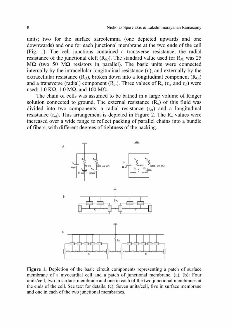
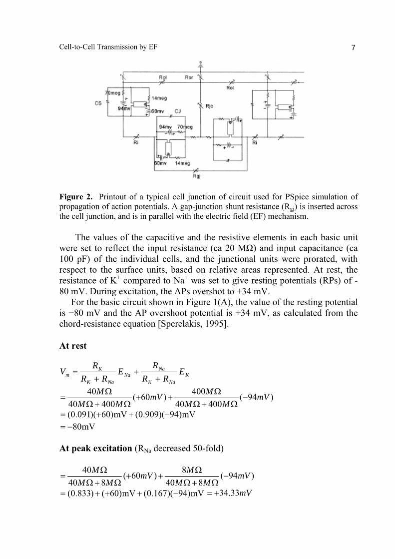
units; two for the surface sarcolemma (one depicted upwards and one downwards) and one for each junctional membrane at the two ends of the cell (Fig. 1). The cell junctions contained a transverse resistance, the radial resistance of the junctional cleft (RJC). The standard value used for RJC was 25 MΩ (two 50 MΩ resistors in parallel). The basic units were connected internally by the intracellular longitudinal resistance (ri), and externally by the extracellular resistance (RO), broken down into a longitudinal component (ROl) and a transverse (radial) component (Ror). Three values of Ro (ror and rol) were used: 1.0 KΩ, 1.0 MΩ, and 100 MΩ. The chain of cells was assumed to be bathed in a large volume of Ringer solution connected to ground. The external resistance (Ro) of this fluid was divided into two components: a radial resistance (ror) and a longitudinal resistance (rol). This arrangement is depicted in Figure 2. The Ro values were increased over a wide range to reflect packing of parallel chains into a bundle of fibers, with different degrees of tightness of the packing.
Figure 1. Depiction of the basic circuit components representing a patch of surface membrane of a myocardial cell and a patch of junctional membrane. (a), (b): Four units/cell, two in surface membrane and one in each of the two junctional membranes at the ends of the cell. See text for details. (c): Seven units/cell, five in surface membrane and one in each of the two junctional membranes.
Cell-to-Cell Transmission by EF 7
Figure 2. Printout of a typical cell junction of circuit used for PSpice simulation of propagation of action potentials. A gap-junction shunt resistance (Rgj) is inserted across the cell junction, and is in parallel with the electric field (EF) mechanism.
The values of the capacitive and the resistive elements in each basic unit were set to reflect the input resistance (ca 20 MΩ) and input capacitance (ca 100 pF) of the individual cells, and the junctional units were prorated, with respect to the surface units, based on relative areas represented. At rest, the resistance of K+ compared to Na+ was set to give resting potentials (RPs) of -80 mV. During excitation, the APs overshot to +34 mV. For the basic circuit shown in Figure 1(A), the value of the resting potential is −80 mV and the AP overshoot potential is +34 mV, as calculated from the chord-resistance equation [Sperelakis, 1995]. At rest
KNaK
NaNa
NaK
Km E
RRR
ERR
RV
++
+=
40 400( 60 ) ( 94 )40 400 40 400
M MmV mVM M M M
Ω Ω= + + −
Ω+ Ω Ω+ Ω
(0.091)( 60)mV (0.909)( 94)mV= + + − 80mV= −
At peak excitation (RNa decreased 50-fold)
40 8( 60 ) ( 94 )40 8 40 8
M MmV mVM M M M
Ω Ω= + + −
Ω+ Ω Ω+ Ω
(0.833) ( 60)mV (0.167)( 94)mV= + + + − mV33.34+=
Nicholas Sperelakis & Lakshminarayanan Ramasamy 8
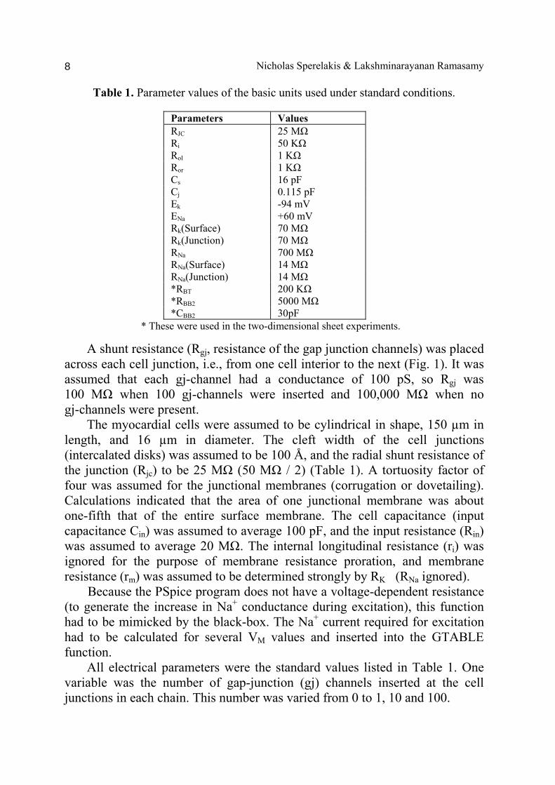
Table 1. Parameter values of the basic units used under standard conditions.
Parameters Values RJC 25 MΩ Ri 50 KΩ Rol 1 KΩ Ror 1 KΩ Cs 16 pF Cj 0.115 pF Ek -94 mV ENa +60 mV Rk(Surface) 70 MΩ Rk(Junction) 70 MΩ RNa 700 MΩ RNa(Surface) 14 MΩ RNa(Junction) 14 MΩ *RBT 200 KΩ *RBB2 5000 MΩ *CBB2 30pF
* These were used in the two-dimensional sheet experiments.
A shunt resistance (Rgj, resistance of the gap junction channels) was placed across each cell junction, i.e., from one cell interior to the next (Fig. 1). It was assumed that each gj-channel had a conductance of 100 pS, so Rgj was 100 MΩ when 100 gj-channels were inserted and 100,000 MΩ when no gj-channels were present.
The myocardial cells were assumed to be cylindrical in shape, 150 µm in length, and 16 µm in diameter. The cleft width of the cell junctions (intercalated disks) was assumed to be 100 Å, and the radial shunt resistance of the junction (Rjc) to be 25 MΩ (50 MΩ / 2) (Table 1). A tortuosity factor of four was assumed for the junctional membranes (corrugation or dovetailing). Calculations indicated that the area of one junctional membrane was about one-fifth that of the entire surface membrane. The cell capacitance (input capacitance Cin) was assumed to average 100 pF, and the input resistance (Rin) was assumed to average 20 MΩ. The internal longitudinal resistance (ri) was ignored for the purpose of membrane resistance proration, and membrane resistance (rm) was assumed to be determined strongly by RK (RNa ignored). Because the PSpice program does not have a voltage-dependent resistance (to generate the increase in Na+ conductance during excitation), this function had to be mimicked by the black-box. The Na+ current required for excitation had to be calculated for several VM values and inserted into the GTABLE function.
All electrical parameters were the standard values listed in Table 1. One variable was the number of gap-junction (gj) channels inserted at the cell junctions in each chain. This number was varied from 0 to 1, 10 and 100.
Cell-to-Cell Transmission by EF 9
The longitudinal average propagation velocity (θ) was calculated from the measured TPT, assuming a cell length of 150 µm, from the following equation:
scmmssmsTPT
junccmjunc //10)(
/100.1593
3
=×××
=Θ−
−
The operation of the PSpice program is very complex, and it is not
necessary to present those details here. The reader is referred to the User Manual from the Cadence program. In addition, the following books are very helpful in understanding the PSpice operation [Nilsson, 2000; Tront, 2007]. When the program is working properly, the results are consistent and reliable. A great amount of information about the electric field transmission and propagation can be learned very quickly and conveniently. For example, the cleft potential amplitude and its action to depolarize the post-junctional membrane can be clearly seen. Types of experiments performed
Section A: Electric field mechanism for transfer of excitation at cell junctions of cardiac muscle
Abstract An EF mechanism was proposed by Sperelakis and colleagues for the transmission of excitation between excitable cells. The EF mechanism was first modeled for cardiac muscle [Sperelakis & Mann, 1977] and subsequently refined in a series of papers [Ruffner et al., 1980; Mann et al., 1981; Picone et al., 1991]. The relevant literature from other laboratories was summarized previously in several review articles [Sperelakis & McConnell, 2001, 2002]. The EF model was first developed on a “breadboard” using physical electronic components (e.g., resistors, capacitors, batteries) and was then modeled mathematically by a series of differential equations and matrix equations, and then simulated on a large computer (CDC-6400) [Sperelakis & Mann, 1977]. The results obtained by the two methods agreed very closely. However, these two methods of analysis are quite cumbersome. Therefore, in order to simplify the EF simulation, we wanted to model it on the PSpice program for electrical engineering. In this Section A, we discuss how we succeeded in demonstrating transmission of excitation from cell to cell in cardiac muscle based on EF transmission at the cell junctions. We presented evidence of a large negative cleft potential that developed in the junctional cleft when the pre-junctional membrane fired an AP. This cleft potential

Nicholas Sperelakis & Lakshminarayanan Ramasamy 10
depolarized the post-junctional membrane to threshold. Thus, successful transmission of excitation occurred in the complete absence of gj-channels. Methods In our first set of experiments, one surface unit represented 2.5 times the membrane area of one junctional unit. Thus, as depicted in Figure 1 (A), CJ was 40% of CS, RK (j) is 2.5 times RK (s), and RNa(j) is 2.5 times RNa(s). In a second set of experiments, the number of surface units per cell was increased to five [Figure 1(C)]. Therefore, each unit represents an equal area of membrane (i.e., there were five surface units/cell). Most experiments were done using a chain length of six cells. To make the circuit as simple as possible, all other types of ion channels (e.g., CaL, CaT, Cl−, Na+ slow, KATP, and KCa) were not entered. We focused only on those channels that set the resting potential (RP; −80 mV) and predominate during the rising phase of the action potential (AP; overshoot to +34 mV). That is, we only wanted to inscribe the rising phase of the APs in a chain of six cells to study rapid propagation. The external longitudinal resistance is relatively low, so it was not entered; that is, the chain of cells was assumed to be bathed in a large volume of medium at ground potential. The longitudinal resistance (Rlj) in each junctional cleft was calculated from the following equation to be 14 Ω [for a cleft thickness (L) of 100 Å and a resistivity (ρ) of the cleft fluid of 50 Ω-cm (about the same as Ringer solution)]: R = ρ L / Ax where Ax is the cross-sectional area of the cleft. Therefore, the radial cleft shunt resistance (Rjc) was connected from the center of two 7 Ω resistances to ground [as depicted in Figure 1(C)]. Increasing the longitudinal cleft resistance over a very wide range had no effect on propagation velocity, because there is almost no local-circuit current across the cell junctions. The circuit used for the entire six-cell chain is too large to be illustrated. A stimulating current pulse was applied to the inside of unit 1 of cell 1. The values for the rectangular current pulse were 0.50 ms duration and 0.5 nA amplitude. The voltages were measured across all units, both surface and junctional. In addition, the voltage was measured across RJC (the cleft potential). The values for RNa in each unit were calculated. The relationship between potential (Vm) and resistance was assumed to be sigmoidal between −60 mV and −30 mV. The peak current supplied by the black-box was 1.95 nA at a Vm of 0 mV. Our black-box is a voltage-controlled current source. The black-box requires a table that gives the response of the desired function (current) for different inputs (membrane voltages). It is used in the circuit in place of a
Cell-to-Cell Transmission by EF 11
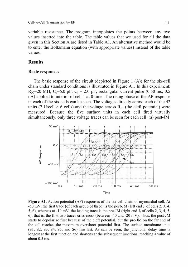
variable resistance. The program interpolates the points between any two values inserted into the table. The table values that we used for all the data given in this Section A are listed in Table A1. An alternative method would be to enter the Boltzmann equation (with appropriate values) instead of the table values. Results Basic responses The basic response of the circuit (depicted in Figure 1 (A)) for the six-cell chain under standard conditions is illustrated in Figure A1. In this experiment: RJC=20 MΩ; Cs=6.0 pF; Cj = 2.0 pF; rectangular current pulse (0.50 ms; 0.5 nA) applied to interior of cell 1 at 0 time. The rising phase of the AP response in each of the six cells can be seen. The voltages directly across each of the 42 units (7 U/cell × 6 cells) and the voltage across RJC (the cleft potential) were measured. Because the five surface units in each cell fired virtually simultaneously, only three voltage traces can be seen for each cell: (a) post-JM
Figure A1. Action potential (AP) responses of the six-cell chain of myocardial cell. At -50 mV, the first trace (of each group of three) is the post-JM (left end Jl of cells 2, 3, 4, 5, 6), whereas at -10 mV, the leading trace is the pre-JM (right end Jr of cells 2, 3, 4, 5, 6); that is, the first two traces criss-cross (between -40 and -20 mV). Thus, the post-JM starts to depolarize first because of the cleft potential, but the pre-JM on the far end of the cell reaches the maximum overshoot potential first. The surface membrane units (S1, S2, S3, S4, S5, and S6) fire last. As can be seen, the junctional delay time is longest at the first junction and shortens at the subsequent junctions, reaching a value of about 0.5 ms.
Nicholas Sperelakis & Lakshminarayanan Ramasamy 12
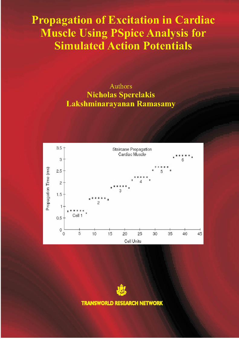
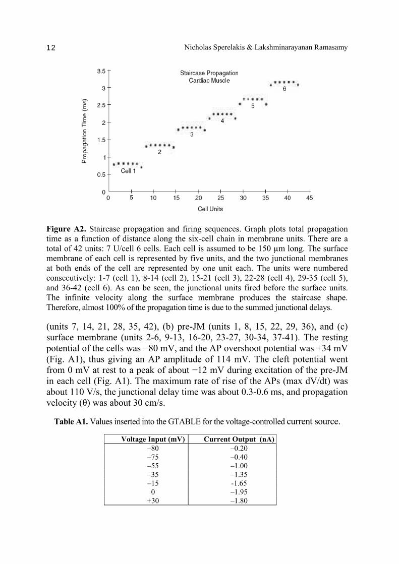
Figure A2. Staircase propagation and firing sequences. Graph plots total propagation time as a function of distance along the six-cell chain in membrane units. There are a total of 42 units: 7 U/cell 6 cells. Each cell is assumed to be 150 µm long. The surface membrane of each cell is represented by five units, and the two junctional membranes at both ends of the cell are represented by one unit each. The units were numbered consecutively: 1-7 (cell 1), 8-14 (cell 2), 15-21 (cell 3), 22-28 (cell 4), 29-35 (cell 5), and 36-42 (cell 6). As can be seen, the junctional units fired before the surface units. The infinite velocity along the surface membrane produces the staircase shape. Therefore, almost 100% of the propagation time is due to the summed junctional delays. (units 7, 14, 21, 28, 35, 42), (b) pre-JM (units 1, 8, 15, 22, 29, 36), and (c) surface membrane (units 2-6, 9-13, 16-20, 23-27, 30-34, 37-41). The resting potential of the cells was −80 mV, and the AP overshoot potential was +34 mV (Fig. A1), thus giving an AP amplitude of 114 mV. The cleft potential went from 0 mV at rest to a peak of about −12 mV during excitation of the pre-JM in each cell (Fig. A1). The maximum rate of rise of the APs (max dV/dt) was about 110 V/s, the junctional delay time was about 0.3-0.6 ms, and propagation velocity (θ) was about 30 cm/s.
Table A1. Values inserted into the GTABLE for the voltage-controlled current source.
Voltage Input (mV) Current Output (nA)–80 –0.20 –75 –0.40 –55 –1.00 –35 –1.35 –15 -1.65 0 –1.95
+30 –1.80
Cell-to-Cell Transmission by EF 13
Firing sequence and staircase propagation
The firing sequence of the seven units of each cell is shown in Figure A2. As can be seen, in cell 1, the pre-JM (unit 7) fired before the post-JM (unit 1), which fired before the surface units (units 2-6). As stated earlier, all surface units fired virtually simultaneously. The lead time of the pre-JM became less in cell 2 and was further reduced in cell 3 (Fig. A2). In cells 4, 5, and 6, the pre-JM and post-JM of each cell fired almost simultaneously. This behavior pattern of the pre-JM (right end of cell) firing slightly before the post-JM (left end of cell) was also observed in the mathematical model [Picone et al., 1991]. The total elapsed time to firing (to 50% of AP amplitude) of the 42 units is listed in Table A2. The graphic plot of propagation time as a function of distance along the chain of six cells (each cell length assumed to be 150 μm) also illustrates the staircase propagation (Fig. A2) [Sperelakis & Ramasamy, 2002]. That is, the shape of the plot is like a staircase. The flat part of each step represents the long surface membrane of each cell. The sharp rise of each step represents the very short (e.g., 100 Å) cell junction gap. As shown, the overall propagation time consists almost entirely of the junctional delay times summed. That is, almost all of the propagation time is due to the junctional transmission process. The velocity of propagation within each cell is almost infinite; i.e., the surface sarcolemma along the cell’s entire length fires simultaneously. Staircase propagation was also observed in the mathematical model [Picone et al., 1991].
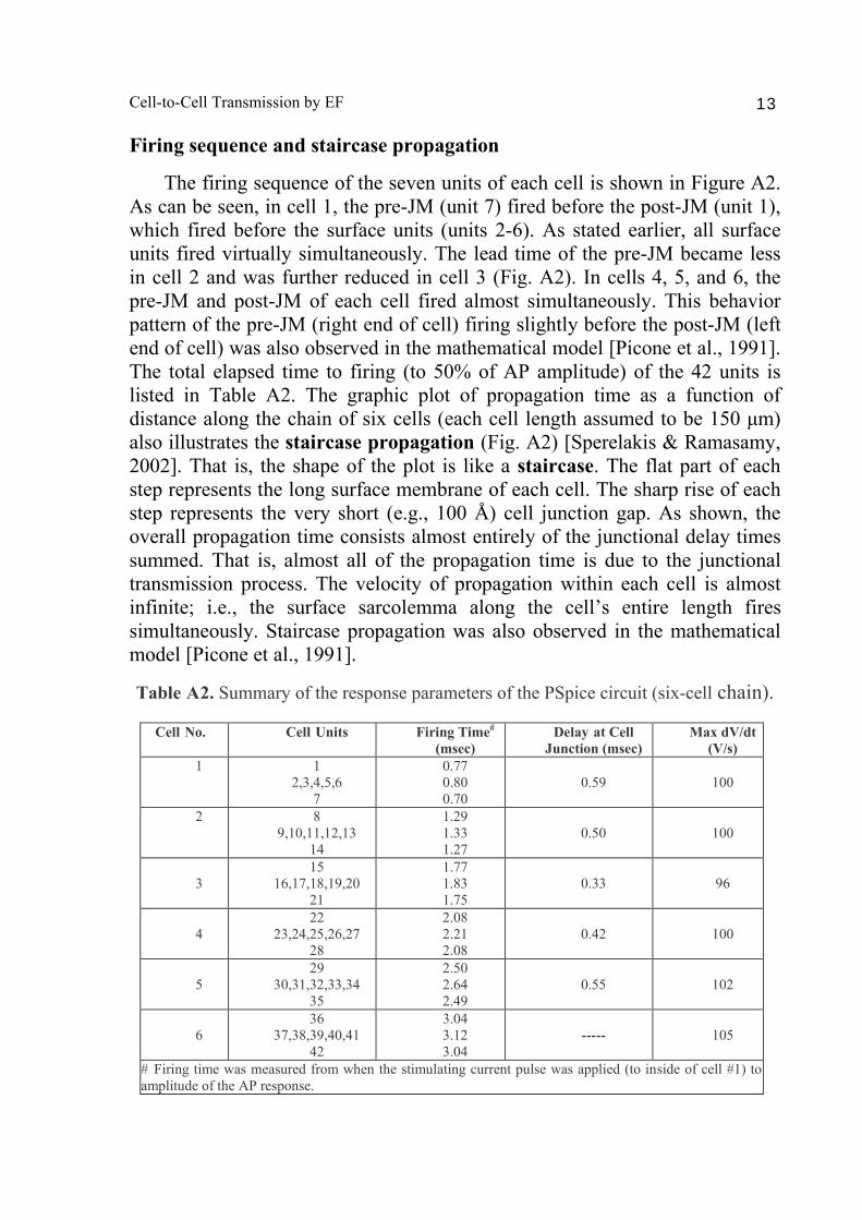
Table A2. Summary of the response parameters of the PSpice circuit (six-cell chain).
Cell No. Cell Units Firing Time# (msec)
Delay at Cell Junction (msec)
Max dV/dt (V/s)
1 1 2,3,4,5,6
7
0.77 0.80 0.70
0.59
100
2 8 9,10,11,12,13
14
1.29 1.33 1.27
0.50
100
3
15 16,17,18,19,20
21
1.77 1.83 1.75
0.33
96
4
22 23,24,25,26,27
28
2.08 2.21 2.08
0.42
100
5
29 30,31,32,33,34
35
2.50 2.64 2.49
0.55
102
6
36 37,38,39,40,41
42
3.04 3.12 3.04
-----
105
# Firing time was measured from when the stimulating current pulse was applied (to inside of cell #1) to amplitude of the AP response.
Nicholas Sperelakis & Lakshminarayanan Ramasamy 14
Junctional delay, cleft potential, and optimal RJC
As stated earlier, the junctional delay time was about 0.3-0.6 ms (Fig. A1, A2 and Table A2). As seen in Figure A1, the junctional delay decreased and leveled off at junctions 1 (cells 1-2), 2 (cells 2-3), 3 (cells 3-4), and 4 (cells 4-5). The delay at junction 5 (cells 5-6) increased again, which we believe is due to an “edge effect.” The delay time is affected by a number of circuit parameters, including magnitude of cleft potential, RJC, Cj , and Cs. In general, the transmission delay is reduced when RJC and the cleft potential are increased and when Cj and Cs are decreased. The negative cleft potential shown in Figure A1 has a peak value of about −12 mV. The magnitude of the cleft potential is affected by a number of circuit parameters, including RJC , Cj , Cs , and the sequence of firing of the units. In general, the cleft potential is larger when RJC is increased and when Cj and Cs are
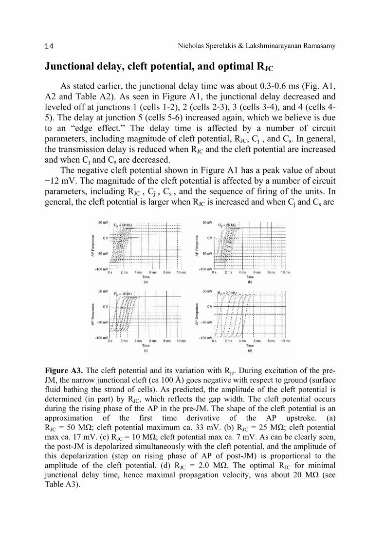
Figure A3. The cleft potential and its variation with Rjc. During excitation of the pre-JM, the narrow junctional cleft (ca 100 Å) goes negative with respect to ground (surface fluid bathing the strand of cells). As predicted, the amplitude of the cleft potential is determined (in part) by RJC, which reflects the gap width. The cleft potential occurs during the rising phase of the AP in the pre-JM. The shape of the cleft potential is an approximation of the first time derivative of the AP upstroke. (a) RJC = 50 MΩ; cleft potential maximum ca. 33 mV. (b) RJC = 25 MΩ; cleft potential max ca. 17 mV. (c) RJC = 10 MΩ; cleft potential max ca. 7 mV. As can be clearly seen, the post-JM is depolarized simultaneously with the cleft potential, and the amplitude of this depolarization (step on rising phase of AP of post-JM) is proportional to the amplitude of the cleft potential. (d) RJC = 2.0 MΩ. The optimal RJC for minimal junctional delay time, hence maximal propagation velocity, was about 20 MΩ (see Table A3).

Cell-to-Cell Transmission by EF 15
decreased. When RJC was increased from our standard 20 MΩ to 50 MΩ and 100 MΩ, the cleft potential increased from −10 mV, to −27 mV, and to −47 mV. The relationship of the cleft potential to depolarization of the post-JM can be clearly seen. The cleft potential instantly depolarizes the post-JM by an equal amount because of its patch-clamp-like action. This produces a prominent step on the rising phase of the AP of the post-cell (e.g., see Fig. A1). The value of RJC for minimum junctional delay, and hence maximal propagation velocity, seemed to pass through a broad optimum. In many experiments, the optimum was 20-30 MΩ. When RJC was reduced below 20 MΩ, θ decreased [Fig. A3 (c)-(d]. All values for delay time are summarized in Table A3. The value of RJC reflects the degree of closeness of the two junctional membranes. Effect of the capacitances (Cs and Cj) The magnitude of the capacitance of the surface membrane (Cs) affected the rise-time of the APs, and hence max dV/dt, when all other parameters were held constant. As expected, based on the RC time constant (τ), lowering Cs increased max dV/dt (Table A4). In agreement with the mathematical model, max dV/dt and Cs had only little effect on θ and junctional delays, especially at Cs values of 5-10 pF (Table A4). The capacitance of the junctional membrane (Cj) affected the junctional delay time more prominently. Lowering Cj decreased the junctional delay and increased θ (Fig. A4). In agreement with the mathematical model, Cj had a pronounced effect on θ, as expected, because propagation time is primarily consumed at the cell junctions. The summary of all the data plotted in Figure A4 shows that the junctional delay increases as Cj is increased and that θ decreases. Effect of variation in membrane excitability on propagation velocity Studies were done on single chains (five cells) of cardiac muscle cells having high, intermediate, and low levels of excitability. Experiments were done with a single chain of five cells. There were no gap junctions between cells within any chain. The GTABLE values we originally used made the myocardial cells somewhat hyper-excitable. Therefore, in the present experiments, the GTABLE values were altered to produce three levels of excitability in the cells: high, intermediate, and low. The present high excitability is the same level of excitability used previously. One key factor determining the amplitude of the negative junctional cleft potential (VJC) was previously shown to be the value of the radial resistance of
Nicholas Sperelakis & Lakshminarayanan Ramasamy 16
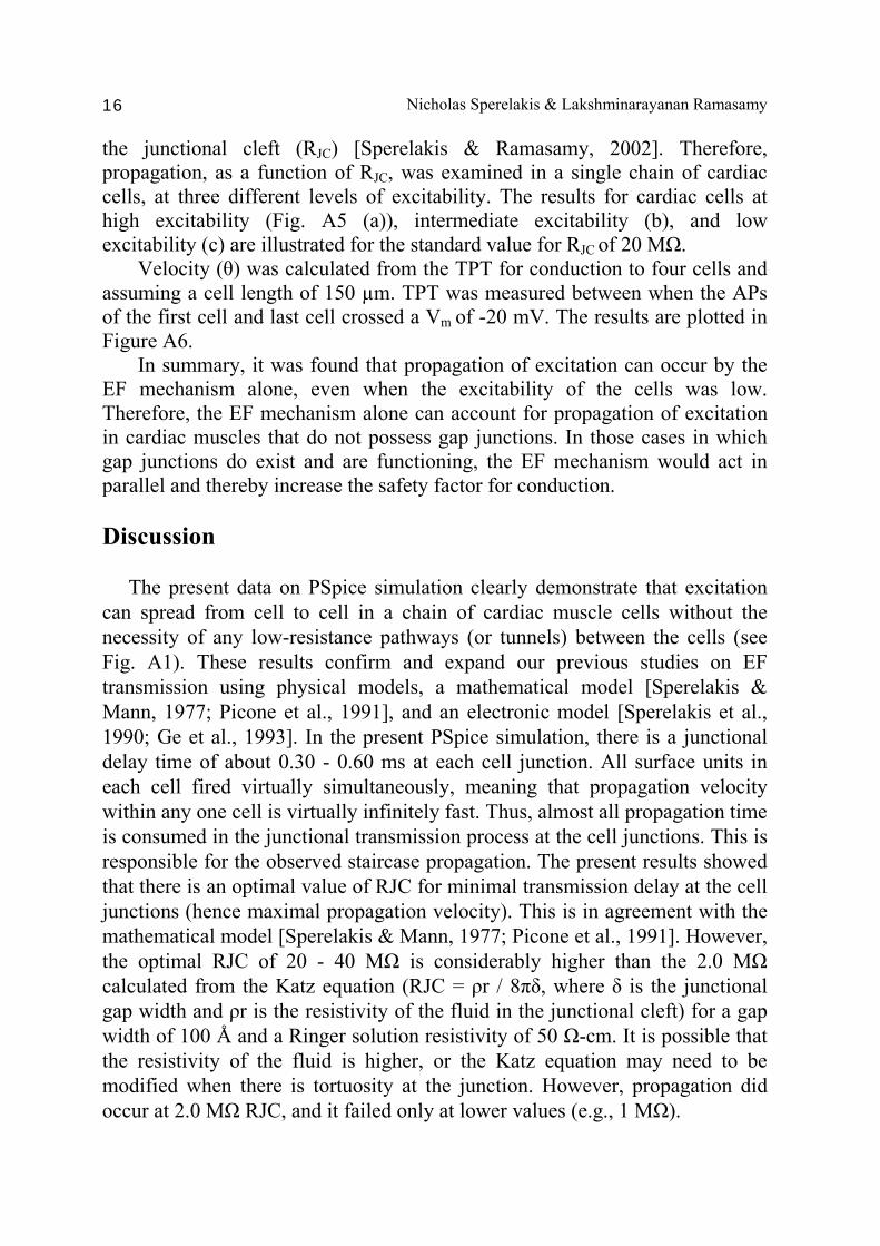
the junctional cleft (RJC) [Sperelakis & Ramasamy, 2002]. Therefore, propagation, as a function of RJC, was examined in a single chain of cardiac cells, at three different levels of excitability. The results for cardiac cells at high excitability (Fig. A5 (a)), intermediate excitability (b), and low excitability (c) are illustrated for the standard value for RJC of 20 MΩ. Velocity (θ) was calculated from the TPT for conduction to four cells and assuming a cell length of 150 µm. TPT was measured between when the APs of the first cell and last cell crossed a Vm of -20 mV. The results are plotted in Figure A6. In summary, it was found that propagation of excitation can occur by the EF mechanism alone, even when the excitability of the cells was low. Therefore, the EF mechanism alone can account for propagation of excitation in cardiac muscles that do not possess gap junctions. In those cases in which gap junctions do exist and are functioning, the EF mechanism would act in parallel and thereby increase the safety factor for conduction. Discussion The present data on PSpice simulation clearly demonstrate that excitation can spread from cell to cell in a chain of cardiac muscle cells without the necessity of any low-resistance pathways (or tunnels) between the cells (see Fig. A1). These results confirm and expand our previous studies on EF transmission using physical models, a mathematical model [Sperelakis & Mann, 1977; Picone et al., 1991], and an electronic model [Sperelakis et al., 1990; Ge et al., 1993]. In the present PSpice simulation, there is a junctional delay time of about 0.30 - 0.60 ms at each cell junction. All surface units in each cell fired virtually simultaneously, meaning that propagation velocity within any one cell is virtually infinitely fast. Thus, almost all propagation time is consumed in the junctional transmission process at the cell junctions. This is responsible for the observed staircase propagation. The present results showed that there is an optimal value of RJC for minimal transmission delay at the cell junctions (hence maximal propagation velocity). This is in agreement with the mathematical model [Sperelakis & Mann, 1977; Picone et al., 1991]. However, the optimal RJC of 20 - 40 MΩ is considerably higher than the 2.0 MΩ calculated from the Katz equation (RJC = ρr / 8πδ, where δ is the junctional gap width and ρr is the resistivity of the fluid in the junctional cleft) for a gap width of 100 Å and a Ringer solution resistivity of 50 Ω-cm. It is possible that the resistivity of the fluid is higher, or the Katz equation may need to be modified when there is tortuosity at the junction. However, propagation did occur at 2.0 MΩ RJC, and it failed only at lower values (e.g., 1 MΩ).
Cell-to-Cell Transmission by EF 17
Table A3. Effect of varying the cleft radial shunt resistance (RJC) on the junctional delay time (between cells 4-5).
RJC (MΩ) Junctional Delay Time (ms) 0.5 Failed 1 1.48 2 0.96 10 0.77 20 0.50 50 0.64
Table A4. Effect of variation in capacitance of surface membrane (Cs) on maximum rate of rise of the action potential (max dV/dt) and on the junctional delay time (between cells 4-5).
Cs (pF) Max dV/dt (V/s) Junctional Delay (ms)
3 169 0.59 4 130 0.50 5 122 0.32 6 102 0.34 7 96 0.32 8 85 0.32 9 76 0.32
Figure A4. Summary graphs of effect of the capacitance of the junctional membranes (Cj) on junctional delay time (a) and on propagation velocity (θ) (b). Cs was held constant at 6 pF. As shown, lowering Cj from 5 pF to 1 pF decreased the delay from 0.88 ms to 0.33 ms, and θ increased from 17 cm/s to 44 cm/s.
Nicholas Sperelakis & Lakshminarayanan Ramasamy 18
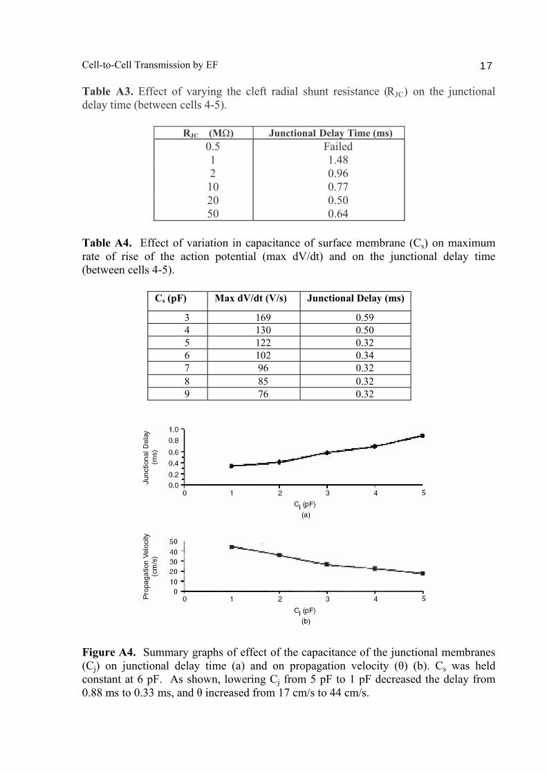
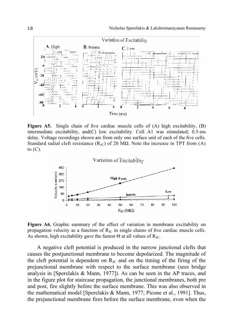
Figure A5. Single chain of five cardiac muscle cells of (A) high excitability, (B) intermediate excitability, and(C) low excitability. Cell A1 was stimulated; 0.5-ms delay. Voltage recordings shown are from only one surface unit of each of the five cells. Standard radial cleft resistance (RJC) of 20 MΩ. Note the increase in TPT from (A) to (C).
Figure A6. Graphic summary of the effect of variation in membrane excitability on propagation velocity as a function of RJC in single chains of five cardiac muscle cells. As shown, high excitability gave the fastest Θ at all values of RJC. A negative cleft potential is produced in the narrow junctional clefts that causes the postjunctional membrane to become depolarized. The magnitude of the cleft potential is dependent on RJC and on the timing of the firing of the prejunctional membrane with respect to the surface membrane (sees bridge analysis in [Sperelakis & Mann, 1977]). As can be seen in the AP traces, and in the figure plot for staircase propagation, the junctional membranes, both pre and post, fire slightly before the surface membrane. This was also observed in the mathematical model [Sperelakis & Mann, 1977; Picone et al., 1991]. Thus, the prejunctional membrane fires before the surface membrane, even when the
Cell-to-Cell Transmission by EF 19
junctional units and surface units were identical in almost all respects (including table values for RNa variation). This leading of the junctional units should become even greater if the junctional units are made more excitable (than the surface units) (by shifting the sigmoidal curve for RNa to the left by about 10 mV). Since we and others have shown (by fluorescent antibody technique) that fast Na+ channels are in higher density in the junctional membranes (intercalated disks) than in the surface membrane [Sperelakis, 1995], the junctional membranes should be more excitable than the surface membranes. The staircase propagation in the EF model causes a discontinuous conduction. This finding is in good agreement with the results of other investigators, in both experimental and theoretical studies. For example, Spach et al. [Spach et al., 1981] showed in 1981 that propagation in normal cardiac muscle was discontinuous in nature. They reported in 1987 similar findings in computer simulations. In theoretical simulations, Diaz et al. [Diaz et al., 1983] concluded in 1983 that continuous cable theory does not apply to propagation in cardiac muscle and that excitation jumps from cell junction to cell junction. These findings were further explored by Rudy and Quan in 1987 [Rudy & Quan, 1987]. A proceedings book was published in 1997 that covers numerous aspects of discontinuous conduction in heart muscle [Spooner et al., 1997]. The mechanism for the transmission of excitation from one cell to the next is not by local-circuit current from the pre-cell to the post-cell. This is clearly evident by examining the voltage across the post-JM. As can be seen in the various figures, the post-JM is not hyperpolarized, as would be requisite if local-circuit current passed through it (IR drop). Rather, the post-JM is depolarized and along the time course dictated by the cleft potential. In addition, if local-circuit current were the mechanism, the post-JM would fire after the surface membrane and not before it. In addition, increasing the longitudinal cleft resistance (Rlj) from 7 Ω to 7 MΩ had no effects whatsoever on propagation velocity. In summary, we modeled propagation in cardiac muscle using the PSpice program. Excitation was shown to transmit from one cell to the next in a chain of cells not connected by low-resistance pathways. The mechanism for the transfer of excitation from one cell to another is by the electric field (negative cleft potential) that develops in the narrow junctional clefts when the prejunctional membrane fires. This negative cleft potential depolarizes the postjunctional membrane by a patch-clamp-like effect. Depolarization of the postjunctional membrane to threshold brings the subsequent distal prejunctional membrane in that cell to threshold, followed by the entire surface membrane. The magnitude of the cleft pot is a function of RJC and the timing of firing. The entire length of each cell’s surface membrane fires virtually

Nicholas Sperelakis & Lakshminarayanan Ramasamy 20
simultaneously, causing staircase propagation, with almost all propagation time being consumed at the cell junctions. The junctional delay time being consumed at the cell junctions. The junctional delay time was about 0.30-0.60 ms and propagation velocity was about 25-40 cm/s. Therefore, the present results provide strong evidence in support of the EF mechanism for cell-to-cell transmission in cardiac muscle. The EF mechanism is an independent method for transmission of excitation from one cell to the next, but it may work in parallel with other mechanisms, such as K+ accumulation and gap-junction tunnels (see discussion [Sperelakis & McConnell, 2001, 2002]). Section B: Combined electric field and gap junctions on propagation of cardiac action potentials
Abstract
Propagation of APs in cardiac muscle was simulated using the PSpice program. Excitation was transmitted from cell to cell along a strand of 6 cells either not connected or connected by low-resistance tunnels (gap-junction channels). A large negative cleft potential (VJC) develops in the narrow junctional cleft when the pre-junctional membrane (pre-JM) fires. VJC depolarizes the postjunctional membrane (post-JM) to threshold. With few connecting tunnels, cell-to-cell transmission by the EF mechanism was facilitated. With many tunnels, propagation was dominated by the low-resistance mechanism, and propagation velocity (θ) became very fast and non-physiological. In conclusion, when the two mechanisms for cell-to-cell transfer of excitation were combined, the two mechanisms facilitated each other in a synergistic manner. When there were many connecting tunnels, the tunnel mechanism was dominant. Background An EF mechanism was first proposed in 1977 by Sperelakis and Mann for the transmission of excitation between cardiac muscle cells. The EF mechanism for propagation was recently modeled on the PSpice program by Sperelakis and Ramasamy (2002) for cardiac muscle, using short chains of 6 or 10 cells. Although these strands of cells were not connected by low- resistance pathways (gap-junction connexons), propagation occurred nicely by means of the EF that develops in the narrow junctional clefts when the prejunctional membrane (pre-JM) fires an AP. The magnitude of the cleft potential (VJC) that is generated is a function of the magnitude of the RJC. When the external resistance (Ro) was varied over a very wide range, It was found that propagation can occur at very high external resistance, indicating
Cell-to-Cell Transmission by EF 21
that local-circuit current is not important for transmission from cell to cell [Sperelakis & Murali, 2003]. When the EF mechanism was combined with the gap junction mechanism (this was performed by placing a variable shunt resistor across each junction), it was found that the two mechanisms were facilitory. When there were many connecting tunnels, the tunnel mechanism became dominant. Methods The values for the circuit parameters used under standard conditions are listed in Table 1 for both the surface units and junctional units. There was a V-controlled current source (our “black-box”) in each of the basic circuit units (Fig. 2). The current output of the black-box at various membrane voltages are listed in Table A1. The currents were calculated assuming a sigmoidal relationship between membrane voltage and resistance between -60 mV and -30 mV.
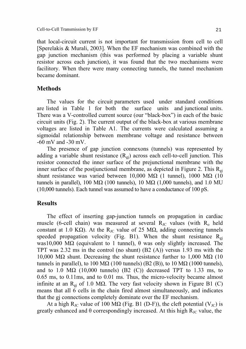
The presence of gap junction connexons (tunnels) was represented by adding a variable shunt resistance (Rgj) across each cell-to-cell junction. This resistor connected the inner surface of the prejunctional membrane with the inner surface of the postjunctional membrane, as depicted in Figure 2. This Rgj shunt resistance was varied between 10,000 MΩ (1 tunnel), 1000 MΩ (10 tunnels in parallel), 100 MΩ (100 tunnels), 10 MΩ (1,000 tunnels), and 1.0 MU (10,000 tunnels). Each tunnel was assumed to have a conductance of 100 pS. Results The effect of inserting gap-junction tunnels on propagation in cardiac muscle (6-cell chain) was measured at several RJC values (with Ro held constant at 1.0 KΩ). At the RJC value of 25 MΩ, adding connecting tunnels speeded propagation velocity (Fig. B1). When the shunt resistance Rgj was10,000 MΩ (equivalent to 1 tunnel), θ was only slightly increased. The TPT was 2.32 ms in the control (no shunt) (B2 (A)) versus 1.93 ms with the 10,000 MΩ shunt. Decreasing the shunt resistance further to 1,000 MΩ (10 tunnels in parallel), to 100 MΩ (100 tunnels) (B2 (B)), to 10 MΩ (1000 tunnels), and to 1.0 MΩ (10,000 tunnels) (B2 (C)) decreased TPT to 1.33 ms, to 0.65 ms, to 0.11ms, and to 0.01 ms. Thus, the micro-velocity became almost infinite at an Rgj of 1.0 MΩ. The very fast velocity shown in Figure B1 (C) means that all 6 cells in the chain fired almost simultaneously, and indicates that the gj connections completely dominate over the EF mechanism. At a high RJC value of 100 MΩ (Fig. B1 (D-F)), the cleft potential (VJC) is greatly enhanced and θ correspondingly increased. At this high RJC value, the
Nicholas Sperelakis & Lakshminarayanan Ramasamy 22
Figure B1. Effect of inserting gap-junction channels on propagation in cardiac muscle (6-cell chain), at the standard radial junctional cleft resistance (RJC) of 25 MΩ and standard external resistance (Ro; ror and rol) of 1.0 KΩ. (A) Control (no gap-junction shunt resistance (Rgj) or ∞ Rgj). Total propagation time (TPT) over the 6 cells was 2.32 ms. The maximum rate of rise of the AP (dV/dt max) was about 185 V/s. (B) Rgj = 100 MΩ (100 tunnels). TPT = 0.65 ms. (C) Rgj = 1.0 MΩ (10,000 tunnels). TPT = ca. 0.01 ms. The AP responses of the 6 cells occurred nearly simultaneously. dV/dt max was about 250 v/s. Stimulus (0.5ms; 0.5 nA) was applied to inside of cell #1 at zero time. effect of the shunt Rgj was slightly reduced. When Rgj was decreased to 1,000 MΩ, 100 MΩ, 10 MΩ, and 1.0 MΩ, propagation occurred over the entire chain at increasing velocities. TPT was 1.40 ms, 0.64 ms, 0.10 ms, and <0.01 ms. Discussion Discontinuous conduction is caused by a high junctional resistance, and one evidence for the latter is a high input resistance measured for a myocardial cell within a bundle by Sperelakis and colleagues (see refs [Sperelakis & McConnell, 2001, 2002]). Others have observed similar high values in isolated cell pairs of about 25 MΩ [Weingart & Metzger, 1988; Joyner et al., 1991]. More evidence for high junctional resistance is the short length constant, of about one cell length, measured by Sperelakis and colleagues (see discussion in refs [Sperelakis & McConnell, 2001, 2002]). Kleber et al. (1987) reported a λ value of about 350 µm, a value much shorter than that they had previously reported [Weidmann, 1966].
Cell-to-Cell Transmission by EF 23
The present results demonstrated that insertion of junctional tunnels has a pronounced effect on propagation velocity in cardiac muscle. Even insertion of only 1 tunnel had a significant effect. When 10,000 tunnels were inserted, the APs of all cells in the chain occurred nearly simultaneously. This means that the entire group of cells behaved electrically as one cell. With greater shunting (lower Rgj), the local-circuit current transmission between cells dominates over the EF mechanism. Henriquez et al. (2001) did a computer simulation study on a gj model [Vogel & Weingart, 1998], coupling 300 myocardial cells in a linear strand. Conduction velocity was very slow and junctional delay was very long when the junctional resistance was 70–180 MΩ (equivalent to about 150–50 channels). The study of Henriquez et al. (2001) did not consider the role played by the junctional cleft potential, which would allow physiological velocity in the complete absence of gap junctions. This oversight was corrected in a paper by Kucera et al. (2002) in which they incorporated our EF mechanism into their gj model for propagation in cardiac muscle, along with our demonstration that the ID membranes have a higher density of fast Na+ channels than the surface membrane (see refs [Sperelakis & McConnell, 2001, 2002]). Their modeling confirmed the presence of a large negative junctional cleft potential that produced a supra-threshold depolarization of the post-JM, and they concluded that the EF mechanism facilitates transmission from cell to cell and increases conduction velocity. Computer simulation studies on propagation in cardiac muscle were also conducted by Rudy and colleagues [Shaw & Rudy, 1997; Rudy, 2001] Velocity could be reduced to 0.26 cm/s before failure occurred, meaning that propagation can occur with very high junctional resistance, as proposed in our present study. If they had introduced the role played by the junctional cleft potential, their results would probably be in closer agreement with the present findings. The cleft potential was incorporated in a simulation by Hogues et al. (1992). The EF mechanism is an electrical mechanism for the rapid transfer of excitation from one cell to the next, without the requirement of gj channels being present and open. The myocardium of many vertebrates does not even contain gjs. Since gj channels can be closed and made nonfunctioning by certain factors, such as elevated [CaI] that occurs during contraction, this mechanism is labile. In contrast, the EF mechanism depends only on the junctional membranes being excitable and firing slightly before the surface membrane. This has been shown to occur in our mathematical model [Sperelakis & Mann, 1977] and PSpice model [Sperelakis & Ramasamy, 2002; Sperelakis & Murali, 2003]. The shorter the junctional gap, the greater is the negative cleft potential, and hence the shorter is the junctional delay and the
Nicholas Sperelakis & Lakshminarayanan Ramasamy 24
faster the propagation velocity. The sum of the junctional delays accounts for almost all of the propagation time down a strand of cells. The EF mechanism accounts very nicely for the experimental fact that propagation in cardiac muscle is discontinuous in nature. The present study suggests that, if many gj channels are simultaneously open, propagation velocity becomes very fast and non-physiological. The EF mechanism is consistent with recent reports showing that propagation velocity in heart is only moderately slowed in the connexins-43 and connexin-40 knockout mice [Tamaddon et al., 2000; Vaidya et al., 2001]. In summary, the present results show that the EF mechanism and the gj mechanism can act in concert to improve and stabilize propagation in cardiac muscle. Insertion of only one gap-junction channel is capable of increasing propagation velocity and of enabling complete propagation in cases where failure had occurred at some junction. Insertion of more and more tunnels produced faster and faster velocities. The propagation velocities quickly far exceeded the physiological values in the strongly coupled cases. Therefore, in cases where gap junctions are present morphologically, only a small fraction of the channels may be open and functioning at any given instant in time. The presence of the two mechanisms in parallel increases the safety factor for propagation. Section C: Transverse propagation in a two-dimensional sheet of myocardial cells Abstract Transverse propagation in a two-dimensional sheet of cardiac muscle was examined. Longitudinal propagation within each chain, and transverse propagation between parallel chains, occurred even when there were no gj channels inserted between the simulated myocardial cells either longitudinally or transversely. There were pronounced edge (boundary) effects and end-effects even within single chains. Transverse velocity increased with increase in model size. We examined boundary effects on transverse propagation velocity when the length of the chains was held constant at 10 cells and the number of parallel chains was varied from 3 to 5, to 7, to 10, and to 20. The number of gj channels was either zero, both longitudinally and transversely (0/0), or 100/100. Some experiments were also made at 100/ 0, 1/1, and 10/10. Transverse velocity and overall velocity (both longitudinal and transverse components) was calculated from the measured TPT, i.e., the elapsed time between when the first AP and the last AP crossed the zero potential level. The transverse g-j channels were placed only at the ends of each chain, such that
Cell-to-Cell Transmission by EF 25
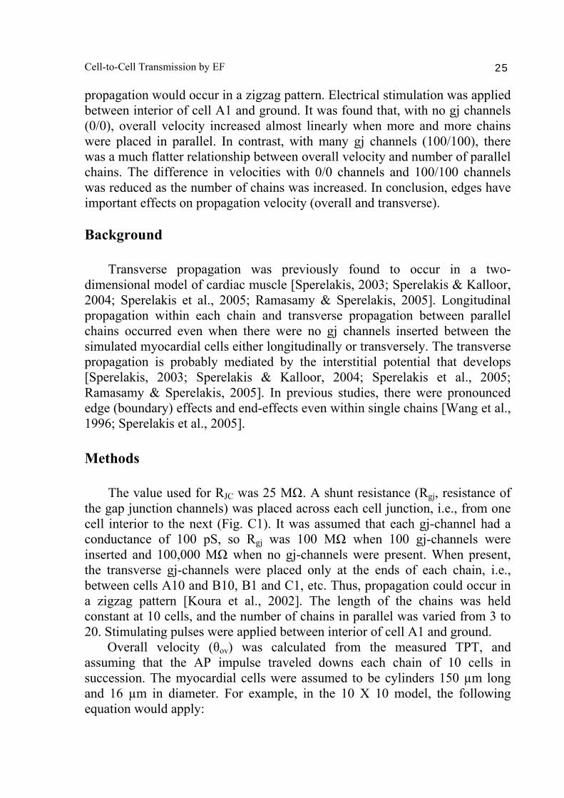
propagation would occur in a zigzag pattern. Electrical stimulation was applied between interior of cell A1 and ground. It was found that, with no gj channels (0/0), overall velocity increased almost linearly when more and more chains were placed in parallel. In contrast, with many gj channels (100/100), there was a much flatter relationship between overall velocity and number of parallel chains. The difference in velocities with 0/0 channels and 100/100 channels was reduced as the number of chains was increased. In conclusion, edges have important effects on propagation velocity (overall and transverse). Background Transverse propagation was previously found to occur in a two-dimensional model of cardiac muscle [Sperelakis, 2003; Sperelakis & Kalloor, 2004; Sperelakis et al., 2005; Ramasamy & Sperelakis, 2005]. Longitudinal propagation within each chain and transverse propagation between parallel chains occurred even when there were no gj channels inserted between the simulated myocardial cells either longitudinally or transversely. The transverse propagation is probably mediated by the interstitial potential that develops [Sperelakis, 2003; Sperelakis & Kalloor, 2004; Sperelakis et al., 2005; Ramasamy & Sperelakis, 2005]. In previous studies, there were pronounced edge (boundary) effects and end-effects even within single chains [Wang et al., 1996; Sperelakis et al., 2005]. Methods The value used for RJC was 25 MΩ. A shunt resistance (Rgj, resistance of the gap junction channels) was placed across each cell junction, i.e., from one cell interior to the next (Fig. C1). It was assumed that each gj-channel had a conductance of 100 pS, so Rgj was 100 MΩ when 100 gj-channels were inserted and 100,000 MΩ when no gj-channels were present. When present, the transverse gj-channels were placed only at the ends of each chain, i.e., between cells A10 and B10, B1 and C1, etc. Thus, propagation could occur in a zigzag pattern [Koura et al., 2002]. The length of the chains was held constant at 10 cells, and the number of chains in parallel was varied from 3 to 20. Stimulating pulses were applied between interior of cell A1 and ground. Overall velocity (θov) was calculated from the measured TPT, and assuming that the AP impulse traveled downs each chain of 10 cells in succession. The myocardial cells were assumed to be cylinders 150 µm long and 16 µm in diameter. For example, in the 10 X 10 model, the following equation would apply:
Nicholas Sperelakis & Lakshminarayanan Ramasamy 26
(100 cells) (150 µm/cell) (100) (15.0 x 10⁻³ cm) θov = ____________________ = ___________________
TPT (ms) TPT (x 10-3 sec)
Then, the transverse velocity (θtr) was calculated from the following equation:
(10 cells) (16 µm/cell) (10) (1.6 x 10⁻³ cm) Θtr = __________________ = _________________
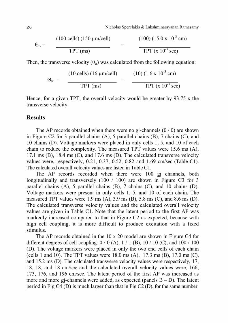
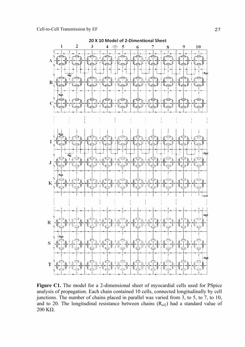
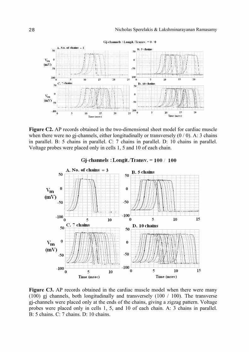
TPT (ms) TPT (x 10-3 sec) Hence, for a given TPT, the overall velocity would be greater by 93.75 x the transverse velocity. Results The AP records obtained when there were no gj-channels (0 / 0) are shown in Figure C2 for 3 parallel chains (A), 5 parallel chains (B), 7 chains (C), and 10 chains (D). Voltage markers were placed in only cells 1, 5, and 10 of each chain to reduce the complexity. The measured TPT values were 15.6 ms (A), 17.1 ms (B), 18.4 ms (C), and 17.6 ms (D). The calculated transverse velocity values were, respectively, 0.21, 0.37, 0.52, 0.82 and 1.69 cm/sec (Table C1). The calculated overall velocity values are listed in Table C1. The AP records recorded when there were 100 gj channels, both longitudinally and transversely (100 / 100) are shown in Figure C3 for 3 parallel chains (A), 5 parallel chains (B), 7 chains (C), and 10 chains (D). Voltage markers were present in only cells 1, 5, and 10 of each chain. The measured TPT values were 1.9 ms (A), 3.9 ms (B), 5.8 ms (C), and 8.6 ms (D). The calculated transverse velocity values and the calculated overall velocity values are given in Table C1. Note that the latent period to the first AP was markedly increased compared to that in Figure C2 as expected, because with high cell coupling, it is more difficult to produce excitation with a fixed stimulus. The AP records obtained in the 10 x 20 model are shown in Figure C4 for different degrees of cell coupling: 0 / 0 (A), 1 / 1 (B), 10 / 10 (C), and 100 / 100 (D). The voltage markers were placed in only the two end cells of each chain (cells 1 and 10). The TPT values were 18.0 ms (A), 17.3 ms (B), 17.0 ms (C), and 15.2 ms (D). The calculated transverse velocity values were respectively, 17, 18, 18, and 18 cm/sec and the calculated overall velocity values were, 166, 173, 176, and 196 cm/sec. The latent period of the first AP was increased as more and more gj-channels were added, as expected (panels B – D). The latent period in Fig C4 (D) is much larger than that in Fig C2 (D), for the same number
Cell-to-Cell Transmission by EF 27
Figure C1. The model for a 2-dimensional sheet of myocardial cells used for PSpice analysis of propagation. Each chain contained 10 cells, connected longitudinally by cell junctions. The number of chains placed in parallel was varied from 3, to 5, to 7, to 10, and to 20. The longitudinal resistance between chains (Rol2) had a standard value of 200 KΩ.
Nicholas Sperelakis & Lakshminarayanan Ramasamy 28
Figure C2. AP records obtained in the two-dimensional sheet model for cardiac muscle when there were no gj-channels, either longitudinally or transversely (0 / 0). A: 3 chains in parallel. B: 5 chains in parallel. C: 7 chains in parallel. D: 10 chains in parallel. Voltage probes were placed only in cells 1, 5 and 10 of each chain.
Figure C3. AP records obtained in the cardiac muscle model when there were many (100) gj channels, both longitudinally and transversely (100 / 100). The transverse gj-channels were placed only at the ends of the chains, giving a zigzag pattern. Voltage probes were placed only in cells 1, 5, and 10 of each chain. A: 3 chains in parallel. B: 5 chains. C: 7 chains. D: 10 chains.
Cell-to-Cell Transmission by EF 29
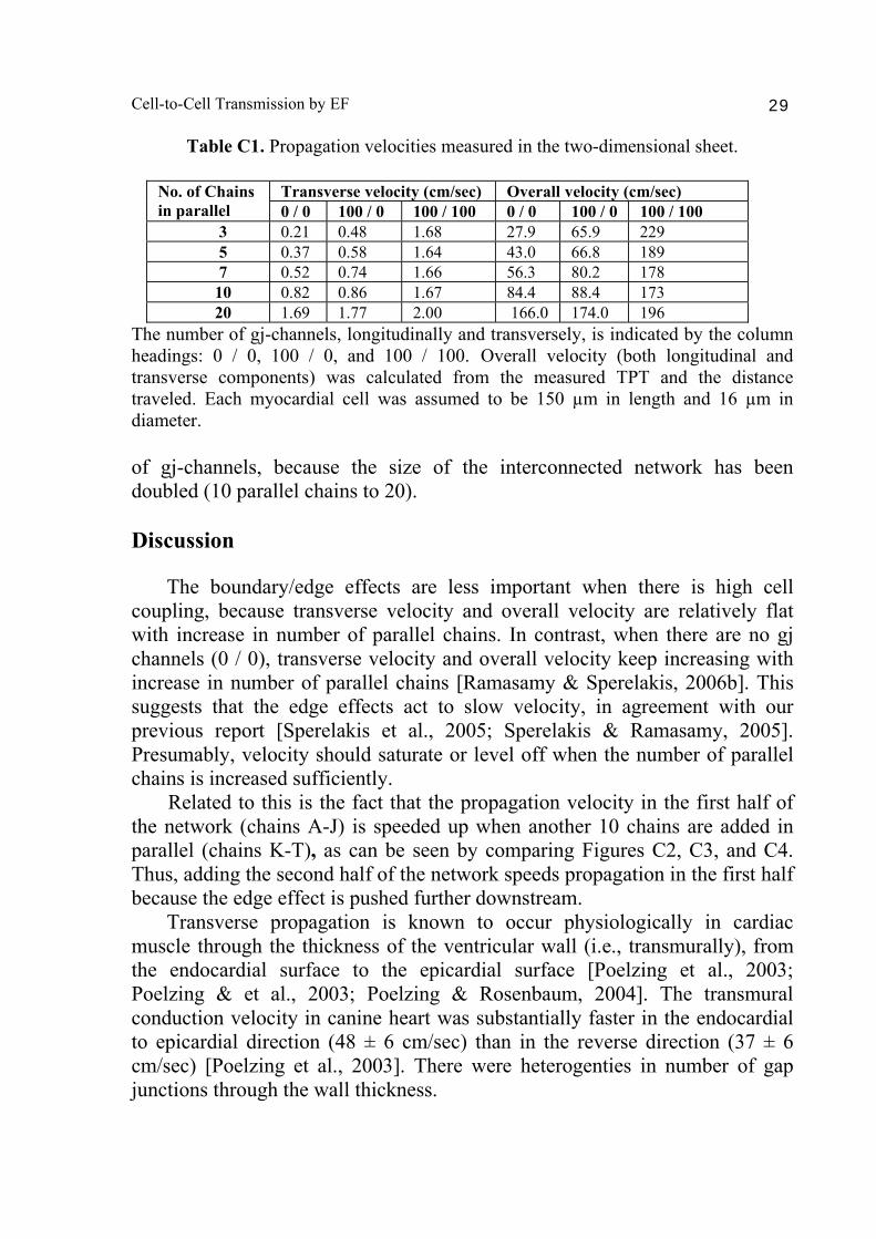
Table C1. Propagation velocities measured in the two-dimensional sheet.
Transverse velocity (cm/sec) Overall velocity (cm/sec) No. of Chains in parallel 0 / 0 100 / 0 100 / 100 0 / 0 100 / 0 100 / 100
3 0.21 0.48 1.68 27.9 65.9 229 5 0.37 0.58 1.64 43.0 66.8 189 7 0.52 0.74 1.66 56.3 80.2 178 10 0.82 0.86 1.67 84.4 88.4 173 20 1.69 1.77 2.00 166.0 174.0 196
The number of gj-channels, longitudinally and transversely, is indicated by the column headings: 0 / 0, 100 / 0, and 100 / 100. Overall velocity (both longitudinal and transverse components) was calculated from the measured TPT and the distance traveled. Each myocardial cell was assumed to be 150 µm in length and 16 µm in diameter. of gj-channels, because the size of the interconnected network has been doubled (10 parallel chains to 20). Discussion The boundary/edge effects are less important when there is high cell coupling, because transverse velocity and overall velocity are relatively flat with increase in number of parallel chains. In contrast, when there are no gj channels (0 / 0), transverse velocity and overall velocity keep increasing with increase in number of parallel chains [Ramasamy & Sperelakis, 2006b]. This suggests that the edge effects act to slow velocity, in agreement with our previous report [Sperelakis et al., 2005; Sperelakis & Ramasamy, 2005]. Presumably, velocity should saturate or level off when the number of parallel chains is increased sufficiently. Related to this is the fact that the propagation velocity in the first half of the network (chains A-J) is speeded up when another 10 chains are added in parallel (chains K-T), as can be seen by comparing Figures C2, C3, and C4. Thus, adding the second half of the network speeds propagation in the first half because the edge effect is pushed further downstream. Transverse propagation is known to occur physiologically in cardiac muscle through the thickness of the ventricular wall (i.e., transmurally), from the endocardial surface to the epicardial surface [Poelzing et al., 2003; Poelzing & et al., 2003; Poelzing & Rosenbaum, 2004]. The transmural conduction velocity in canine heart was substantially faster in the endocardial to epicardial direction (48 ± 6 cm/sec) than in the reverse direction (37 ± 6 cm/sec) [Poelzing et al., 2003]. There were heterogenties in number of gap junctions through the wall thickness.
Nicholas Sperelakis & Lakshminarayanan Ramasamy 30
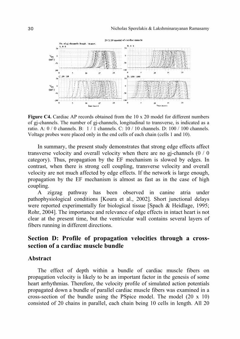
Figure C4. Cardiac AP records obtained from the 10 x 20 model for different numbers of gj-channels. The number of gj-channels, longitudinal to transverse, is indicated as a ratio. A: 0 / 0 channels. B: 1 / 1 channels. C: 10 / 10 channels. D: 100 / 100 channels. Voltage probes were placed only in the end cells of each chain (cells 1 and 10). In summary, the present study demonstrates that strong edge effects affect transverse velocity and overall velocity when there are no gj-channels (0 / 0 category). Thus, propagation by the EF mechanism is slowed by edges. In contrast, when there is strong cell coupling, transverse velocity and overall velocity are not much affected by edge effects. If the network is large enough, propagation by the EF mechanism is almost as fast as in the case of high coupling. A zigzag pathway has been observed in canine atria under pathophysiological conditions [Koura et al., 2002]. Short junctional delays were reported experimentally for biological tissue [Spach & Heidlage, 1995; Rohr, 2004]. The importance and relevance of edge effects in intact heart is not clear at the present time, but the ventricular wall contains several layers of fibers running in different directions. Section D: Profile of propagation velocities through a cross-section of a cardiac muscle bundle Abstract The effect of depth within a bundle of cardiac muscle fibers on propagation velocity is likely to be an important factor in the genesis of some heart arrhythmias. Therefore, the velocity profile of simulated action potentials propagated down a bundle of parallel cardiac muscle fibers was examined in a cross-section of the bundle using the PSpice model. The model (20 x 10) consisted of 20 chains in parallel, each chain being 10 cells in length. All 20
Cell-to-Cell Transmission by EF 31
chains were stimulated simultaneously. The variables were (1) the number of longitudinal gj channels (0, 1, 10, 100), (2) the longitudinal resistance between the parallel chains (Rol2) (reflecting the closeness of the packing of the chains), and (3) the bundle termination resistance at the two ends of the bundle (RBT). It was found that the velocity profile was bell-shaped when there was 0 or only 1 gj-channel. The velocity at the surface of the bundle (θ1 and θ20) was more than double (2.15x) that at the core of the bundle (θ10, θ11). This surface/core ratio of velocities was dependent on the values of Rol2 and RBT. When there were 100 gj-channels, the velocity profile was flat, i.e. the velocity at the core was about the same as that at the surface. Both velocities were more than 10-fold higher than in the absence of gj-channels. Varying Rol2 and RBT had almost no effect. When there were 10 gj-channels, the cross-sectional velocity profile was bullet-shaped, but with a low surface/core ratio. Therefore, when some gj-channels close under pathophysiological conditions, this marked velocity profile could contribute to the genesis of arrhythmias. Background It is predicted from cable theory that velocity of propagation along a fiber is a function of the external resistance of the fluid bathing the fiber: the higher the resistance, the slower the velocity [Sperelakis, 2001]. When parallel fibers are packed within a small-diameter bundle, the outside resistance of fibers near the core should be greater than that of fibers at the surface. Therefore, it is predicted that, by recording electrically at different depths within a myocardial bundle, the propagation velocity of the deeper fibers should be slower than that of the surface fibers. This phenomenon would occur presumably because of the high longitudinal resistance of the interstitial space (or Rol2). Consistent with this, measurements of tissue resistivity in the longitudinal direction vs. transverse (radial) direction showed a marked asymmetry, the resistivity being much higher in the transverse direction [Sperelakis & Macdonald, 1974]. In 1996, Wang et al. carried out a simulation study of a tightly-packed cardiac muscle bundle and found a large interstitial potential. The central (core) fiber exhibited a much slower propagation velocity than the surface fiber when there was no transverse coupling (i.e. no gj-channels) between the parallel fibers. When there was transverse coupling, the central fiber and surface fiber had the same velocity. Other simulation studies of propagation in a cardiac muscle bundle were carried out by Henriquez and Plonsey (1988, 1990a and 1990b). Such slowing of the propagation velocity within the depths of cardiac bundles may be an important factor in the genesis of certain arrhythmias under some pathophysiological conditions, such as transient ischemia. Therefore,
Nicholas Sperelakis & Lakshminarayanan Ramasamy 32
experiments were carried out on a cardiac muscle bundle model, using PSpice to analyze the propagation of simulated cardiac APs at different depths within the bundle. It was found that when there were no or few gj channels, the velocity profile was bell-shaped, with the velocity at the core of the bundle more than 2-fold slower than at the surface. The profile was flat when there were many gj-channels. Therefore, any change in number of gj channels caused by pathophysiological conditions could contribute to certain arrhythmias. Methods The model of cardiac muscle consisted of 20 chains in parallel, each chain being 10 cells in length (20 x 10 model) (Fig. D1), and was intended to represent a cross-sectional plane through a cardiac muscle bundle of small diameter. The top and bottom of the model were made symmetrical, including identical Rol and Ror values, and two grounds to reflect the upper and lower surfaces of the bundle (Fig. D1). Twenty identical electrical stimulators were placed on the left end of the model so that all 20 chains could be stimulated simultaneously. The rectangular current pulses were all identical, i.e. 0.25 nA in amplitude and 0.25 ms in duration, and stimulation was applied intracellularly. Voltage recordings (markers placed intracellularly) were made only from cells 1, 5 and 10 of each chain in order to limit the total number of traces to 60 (20 chains x 3 markers/chain). One variable was the number of gj channels inserted at the cell junctions in each chain. This number was varied from 0 to 1, 10 and 100, with each gj-channel assumed to be 100 pS. Another variable was the value of the longitudinal resistance of the interstitial fluid space between the parallel chains (Rol2). The Rol2 value (standard value of 200 KΩ) reflects the closeness of packing of the chains: the higher the value, the tighter the packing. The third variable was the bundle termination resistance (RBT) at the two ends of the bundle (standard value of 200 KΩ). The longitudinal average propagation velocity (θ) was calculated from the measured TPT, assuming a cell length of 150 µm, from the following equation:
scmmssmsTPT
junccmjunc //10)(
/100.1593
3
=×××
=Θ−
−
Results With 0 gj-channels, the TPT for the impulses to reach cell #10 of each chain are plotted in Figure D2 (A). Note that this curve is bell-shaped, and TPT
Cell-to-Cell Transmission by EF 33
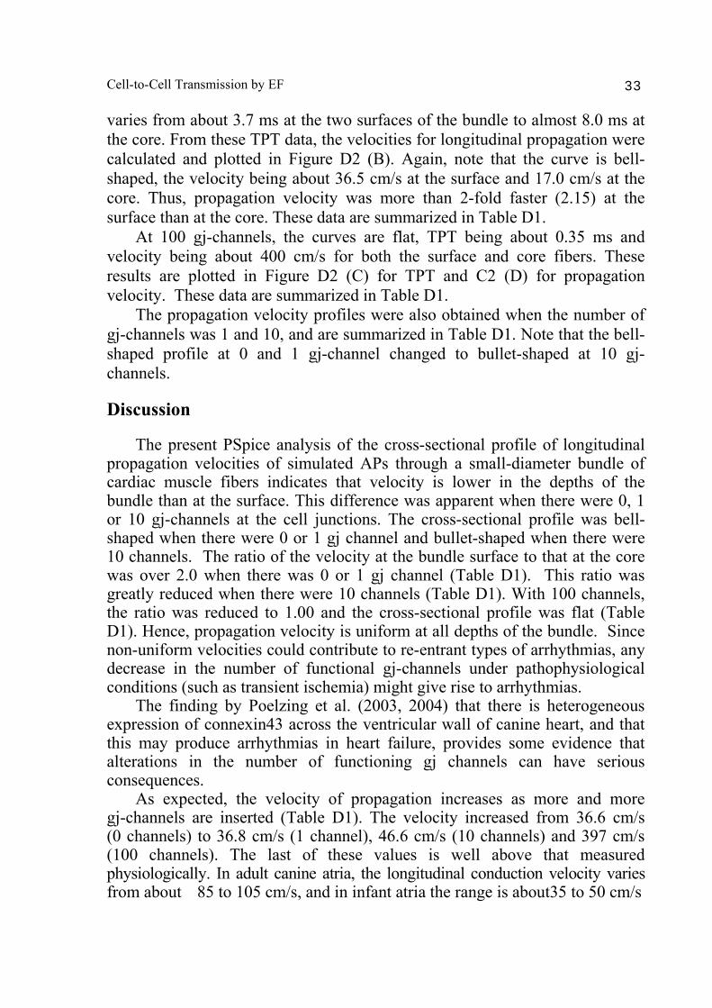
varies from about 3.7 ms at the two surfaces of the bundle to almost 8.0 ms at the core. From these TPT data, the velocities for longitudinal propagation were calculated and plotted in Figure D2 (B). Again, note that the curve is bell-shaped, the velocity being about 36.5 cm/s at the surface and 17.0 cm/s at the core. Thus, propagation velocity was more than 2-fold faster (2.15) at the surface than at the core. These data are summarized in Table D1. At 100 gj-channels, the curves are flat, TPT being about 0.35 ms and velocity being about 400 cm/s for both the surface and core fibers. These results are plotted in Figure D2 (C) for TPT and C2 (D) for propagation velocity. These data are summarized in Table D1.
The propagation velocity profiles were also obtained when the number of gj-channels was 1 and 10, and are summarized in Table D1. Note that the bell-shaped profile at 0 and 1 gj-channel changed to bullet-shaped at 10 gj-channels.
Discussion The present PSpice analysis of the cross-sectional profile of longitudinal propagation velocities of simulated APs through a small-diameter bundle of cardiac muscle fibers indicates that velocity is lower in the depths of the bundle than at the surface. This difference was apparent when there were 0, 1 or 10 gj-channels at the cell junctions. The cross-sectional profile was bell-shaped when there were 0 or 1 gj channel and bullet-shaped when there were 10 channels. The ratio of the velocity at the bundle surface to that at the core was over 2.0 when there was 0 or 1 gj channel (Table D1). This ratio was greatly reduced when there were 10 channels (Table D1). With 100 channels, the ratio was reduced to 1.00 and the cross-sectional profile was flat (Table D1). Hence, propagation velocity is uniform at all depths of the bundle. Since non-uniform velocities could contribute to re-entrant types of arrhythmias, any decrease in the number of functional gj-channels under pathophysiological conditions (such as transient ischemia) might give rise to arrhythmias. The finding by Poelzing et al. (2003, 2004) that there is heterogeneous expression of connexin43 across the ventricular wall of canine heart, and that this may produce arrhythmias in heart failure, provides some evidence that alterations in the number of functioning gj channels can have serious consequences. As expected, the velocity of propagation increases as more and more gj-channels are inserted (Table D1). The velocity increased from 36.6 cm/s (0 channels) to 36.8 cm/s (1 channel), 46.6 cm/s (10 channels) and 397 cm/s (100 channels). The last of these values is well above that measured physiologically. In adult canine atria, the longitudinal conduction velocity varies from about 85 to 105 cm/s, and in infant atria the range is about35 to 50 cm/s
Nicholas Sperelakis & Lakshminarayanan Ramasamy 34
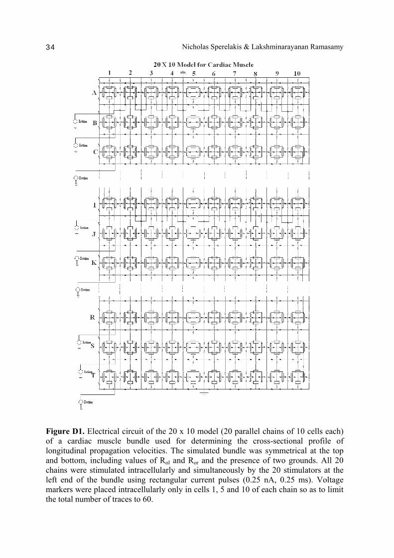
Figure D1. Electrical circuit of the 20 x 10 model (20 parallel chains of 10 cells each) of a cardiac muscle bundle used for determining the cross-sectional profile of longitudinal propagation velocities. The simulated bundle was symmetrical at the top and bottom, including values of Rol and Ror and the presence of two grounds. All 20 chains were stimulated intracellularly and simultaneously by the 20 stimulators at the left end of the bundle using rectangular current pulses (0.25 nA, 0.25 ms). Voltage markers were placed intracellularly only in cells 1, 5 and 10 of each chain so as to limit the total number of traces to 60.
Cell-to-Cell Transmission by EF 35
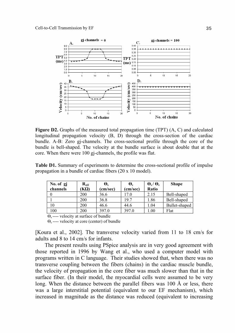
Figure D2. Graphs of the measured total propagation time (TPT) (A, C) and calculated longitudinal propagation velocity (B, D) through the cross-section of the cardiac bundle. A-B: Zero gj-channels. The cross-sectional profile through the core of the bundle is bell-shaped. The velocity at the bundle surface is about double that at the core. When there were 100 gj-channels, the profile was flat. Table D1. Summary of experiments to determine the cross-sectional profile of impulse propagation in a bundle of cardiac fibers (20 x 10 model).
No. of gj channels
Rol2 (KΩ)
Θs (cm/sec)
Θc (cm/sec)
Θs / Θc Ratio
Shape
0 200 36.6 17.0 2.15 Bell-shaped 1 200 36.8 19.7 1.86 Bell-shaped 10 200 46.6 44.6 1.04 Bullet-shaped 100 200 397.0 397.0 1.00 Flat
Θs ---- velocity at surface of bundle Θc ---- velocity at core (center) of bundle [Koura et al., 2002]. The transverse velocity varied from 11 to 18 cm/s for adults and 8 to 14 cm/s for infants. The present results using PSpice analysis are in very good agreement with those reported in 1996 by Wang et al., who used a computer model with programs written in C language. Their studies showed that, when there was no transverse coupling between the fibers (chains) in the cardiac muscle bundle, the velocity of propagation in the core fiber was much slower than that in the surface fiber. (In their model, the myocardial cells were assumed to be very long. When the distance between the parallel fibers was 100 Å or less, there was a large interstitial potential (equivalent to our EF mechanism), which increased in magnitude as the distance was reduced (equivalent to increasing
Nicholas Sperelakis & Lakshminarayanan Ramasamy 36
Rol2). When there was strong transverse coupling between the parallel chains, the propagation velocity in the core chain was the same as that in the surface chain. Section E: Propagation velocity in a long single chain of simulated myocardial cells Abstract Propagation of simulated APs was previously studied in short single chains of myocardial cells [Sperelakis & Ramasamy, 2002; Sperelakis, 2003; Ramasamy & Sperelakis, 2005]. The present study was undertaken to examine propagation in a long single chain of cells of various lengths, and with varying numbers of gj channels. Simulations were carried out using the PSpice program. When the EF mechanism was dominant (0, 1, and 10 gj-channels), the longer the chain length, the faster the overall velocity (θov). There seems to be no simple explanation for this phenomenon. In contrast, when the local-circuit current mechanism was dominant (100 gj-channels or more), θov was slightly slowed with lengthening of the chain. Increasing the number of gj channels produced an increase in θov and caused the firing order to become more uniform. The end-effect was more pronounced at longer chain lengths and at greater number of gj channels. Thus, when there were only 0, 1, or 10 gj channels, θov increased with increase in chain length, whereas at 100 gj-channels or higher, θov did not increase with chain length. Background In previous studies, propagation of APs was examined in short chains of cells (e.g., 10 cells long), with the number of gj channels varied from zero to 10,000 [Sperelakis & Mann, 1977; Picone et al., 1991; Sperelakis & Ramasamy, 2002; Sperelakis, 2002]. Propagation of excitation occurred at near-physiological speeds, even when there were no gj channels connecting between the longitudinally-oriented cells [Sperelakis & Ramasamy, 2002]. The mechanism proposed was the relatively large EF that develops in the narrow junctional clefts when the prejunctional membrane fires an AP [Sperelakis & Mann, 1977; Picone et al., 1991; Sperelakis, 1995; Sperelakis & Ramasamy, 2002; Sperelakis, 2002]. Methods We used long single chains of 10, 20, 50, and 100 cells. The 100-cell chain is depicted in Figure E1. All parameters used were those used previously
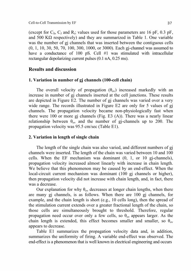
Cell-to-Cell Transmission by EF 37
(except for CS, CJ and Ri; values used for those parameters are 16 pF, 0.3 pF, and 500 KΩ respectively) and they are summarized in Table 1. One variable was the number of gj channels that was inserted between the contiguous cells (0, 1, 10, 30, 50, 70, 100, 300, 1000, or 3000). Each gj-channel was assumed to have a conductance of 100 pS. Cell #1 was stimulated with intracellular rectangular depolarizing current pulses (0.1 nA, 0.25 ms). Results and discussion 1. Variation in number of gj channels (100-cell chain) The overall velocity of propagation (θov) increased markedly with an increase in number of gj channels inserted at the cell junctions. These results are depicted in Figure E2. The number of gj channels was varied over a very wide range. The records illustrated in Figure E2 are only for 5 values of gj channels. The propagation velocity became non-physiologically fast when there were 100 or more gj channels (Fig. E3 (A)). There was a nearly linear relationship between θov and the number of gj-channels up to 200. The propagation velocity was 95.5 cm/sec (Table E1). 2. Variation in length of single chain The length of the single chain was also varied, and different numbers of gj channels were inserted. The length of the chain was varied between 10 and 100 cells. When the EF mechanism was dominant (0, 1, or 10 gj-channels), propagation velocity increased almost linearly with increase in chain length. We believe that this phenomenon may be caused by an end-effect. When the local-circuit current mechanism was dominant (100 gj channels or higher), then propagation velocity did not increase with chain length, and, in fact, there was a decrease. Our explanation for why θov decreases at longer chain lengths, when there are many gj channels, is as follows. When there are 100 gj channels, for example, and the chain length is short (e.g., 10 cells long), then the spread of the stimulation current extends over a greater fractional length of the chain, so those cells are simultaneously brought to threshold. Therefore, regular propagation need occur over only a few cells, so θov appears larger. As the chain length is extended, this effect becomes smaller and smaller, so θov appears to decrease. Table E1 summarizes the propagation velocity data and, in addition, summarizes the uniformity of firing. A variable end-effect was observed. The end-effect is a phenomenon that is well known in electrical engineering and occurs
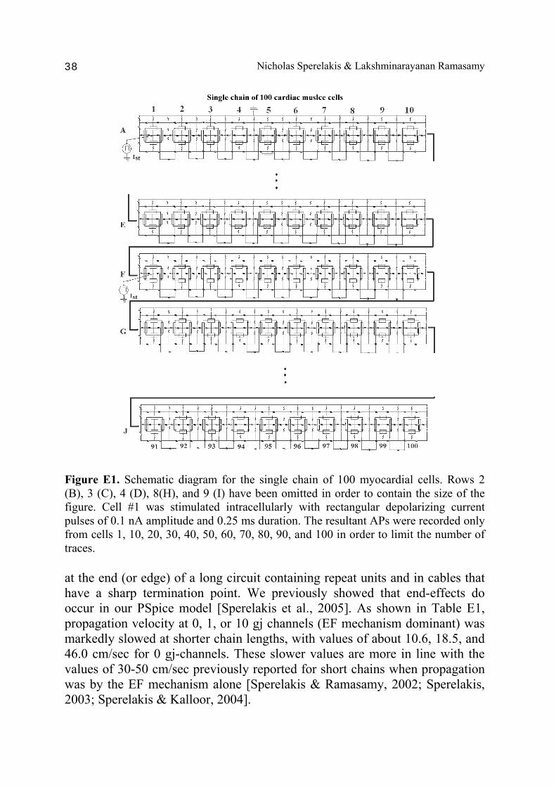
Nicholas Sperelakis & Lakshminarayanan Ramasamy 38
Figure E1. Schematic diagram for the single chain of 100 myocardial cells. Rows 2 (B), 3 (C), 4 (D), 8(H), and 9 (I) have been omitted in order to contain the size of the figure. Cell #1 was stimulated intracellularly with rectangular depolarizing current pulses of 0.1 nA amplitude and 0.25 ms duration. The resultant APs were recorded only from cells 1, 10, 20, 30, 40, 50, 60, 70, 80, 90, and 100 in order to limit the number of traces. at the end (or edge) of a long circuit containing repeat units and in cables that have a sharp termination point. We previously showed that end-effects do occur in our PSpice model [Sperelakis et al., 2005]. As shown in Table E1, propagation velocity at 0, 1, or 10 gj channels (EF mechanism dominant) was markedly slowed at shorter chain lengths, with values of about 10.6, 18.5, and 46.0 cm/sec for 0 gj-channels. These slower values are more in line with the values of 30-50 cm/sec previously reported for short chains when propagation was by the EF mechanism alone [Sperelakis & Ramasamy, 2002; Sperelakis, 2003; Sperelakis & Kalloor, 2004].
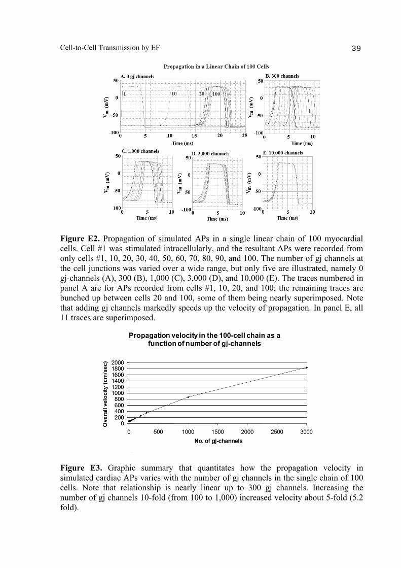
Cell-to-Cell Transmission by EF 39
Figure E2. Propagation of simulated APs in a single linear chain of 100 myocardial cells. Cell #1 was stimulated intracellularly, and the resultant APs were recorded from only cells #1, 10, 20, 30, 40, 50, 60, 70, 80, 90, and 100. The number of gj channels at the cell junctions was varied over a wide range, but only five are illustrated, namely 0 gj-channels (A), 300 (B), 1,000 (C), 3,000 (D), and 10,000 (E). The traces numbered in panel A are for APs recorded from cells #1, 10, 20, and 100; the remaining traces are bunched up between cells 20 and 100, some of them being nearly superimposed. Note that adding gj channels markedly speeds up the velocity of propagation. In panel E, all 11 traces are superimposed.
Figure E3. Graphic summary that quantitates how the propagation velocity in simulated cardiac APs varies with the number of gj channels in the single chain of 100 cells. Note that relationship is nearly linear up to 300 gj channels. Increasing the number of gj channels 10-fold (from 100 to 1,000) increased velocity about 5-fold (5.2 fold).
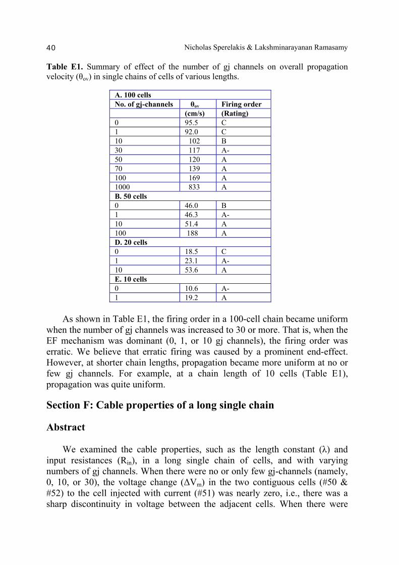
Nicholas Sperelakis & Lakshminarayanan Ramasamy 40
Table E1. Summary of effect of the number of gj channels on overall propagation velocity (θov) in single chains of cells of various lengths.
A. 100 cells No. of gj-channels θov Firing order (cm/s) (Rating) 0 95.5 C 1 92.0 C 10 102 B 30 117 A- 50 120 A 70 139 A 100 169 A 1000 833 A B. 50 cells 0 46.0 B 1 46.3 A- 10 51.4 A 100 188 A D. 20 cells 0 18.5 C 1 23.1 A- 10 53.6 A E. 10 cells 0 10.6 A- 1 19.2 A
As shown in Table E1, the firing order in a 100-cell chain became uniform when the number of gj channels was increased to 30 or more. That is, when the EF mechanism was dominant (0, 1, or 10 gj channels), the firing order was erratic. We believe that erratic firing was caused by a prominent end-effect. However, at shorter chain lengths, propagation became more uniform at no or few gj channels. For example, at a chain length of 10 cells (Table E1), propagation was quite uniform. Section F: Cable properties of a long single chain Abstract We examined the cable properties, such as the length constant (λ) and input resistances (Rin), in a long single chain of cells, and with varying numbers of gj channels. When there were no or only few gj-channels (namely, 0, 10, or 30), the voltage change (ΔVm) in the two contiguous cells (#50 & #52) to the cell injected with current (#51) was nearly zero, i.e., there was a sharp discontinuity in voltage between the adjacent cells. When there were
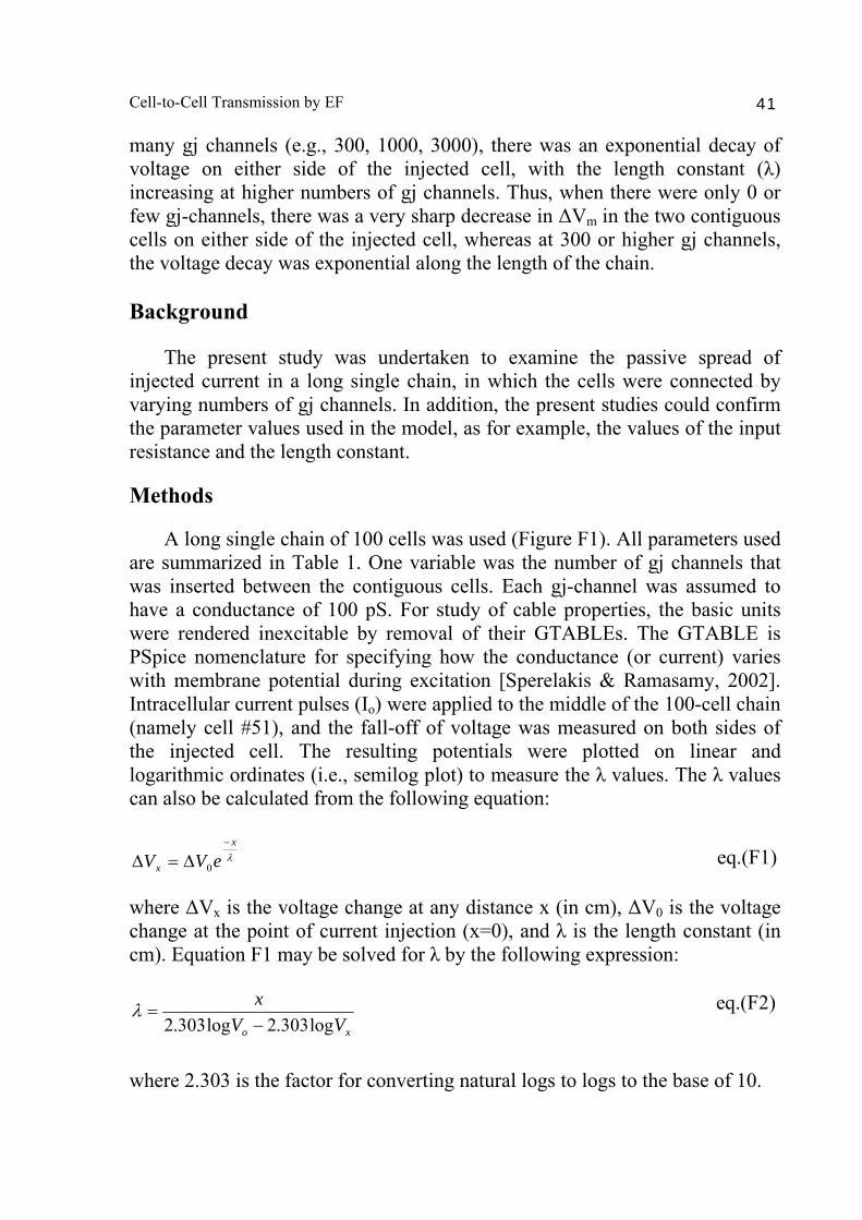
Cell-to-Cell Transmission by EF 41
many gj channels (e.g., 300, 1000, 3000), there was an exponential decay of voltage on either side of the injected cell, with the length constant (λ) increasing at higher numbers of gj channels. Thus, when there were only 0 or few gj-channels, there was a very sharp decrease in ΔVm in the two contiguous cells on either side of the injected cell, whereas at 300 or higher gj channels, the voltage decay was exponential along the length of the chain. Background The present study was undertaken to examine the passive spread of injected current in a long single chain, in which the cells were connected by varying numbers of gj channels. In addition, the present studies could confirm the parameter values used in the model, as for example, the values of the input resistance and the length constant. Methods A long single chain of 100 cells was used (Figure F1). All parameters used are summarized in Table 1. One variable was the number of gj channels that was inserted between the contiguous cells. Each gj-channel was assumed to have a conductance of 100 pS. For study of cable properties, the basic units were rendered inexcitable by removal of their GTABLEs. The GTABLE is PSpice nomenclature for specifying how the conductance (or current) varies with membrane potential during excitation [Sperelakis & Ramasamy, 2002]. Intracellular current pulses (Io) were applied to the middle of the 100-cell chain (namely cell #51), and the fall-off of voltage was measured on both sides of the injected cell. The resulting potentials were plotted on linear and logarithmic ordinates (i.e., semilog plot) to measure the λ values. The λ values can also be calculated from the following equation:
λx
x eVV−
Δ=Δ 0 eq.(F1)
where ΔVx is the voltage change at any distance x (in cm), ΔV0 is the voltage change at the point of current injection (x=0), and λ is the length constant (in cm). Equation F1 may be solved for λ by the following expression:
xo VVx
log303.2log303.2 −=λ eq.(F2)
where 2.303 is the factor for converting natural logs to logs to the base of 10.
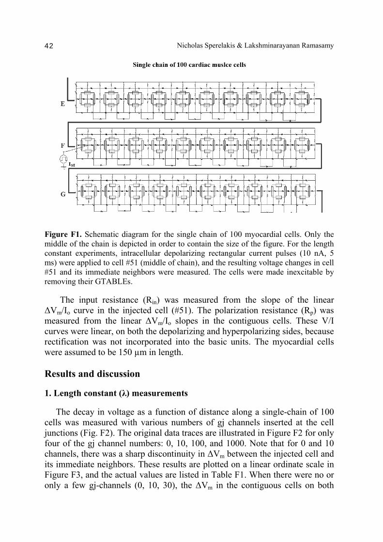
Nicholas Sperelakis & Lakshminarayanan Ramasamy 42
Figure F1. Schematic diagram for the single chain of 100 myocardial cells. Only the middle of the chain is depicted in order to contain the size of the figure. For the length constant experiments, intracellular depolarizing rectangular current pulses (10 nA, 5 ms) were applied to cell #51 (middle of chain), and the resulting voltage changes in cell #51 and its immediate neighbors were measured. The cells were made inexcitable by removing their GTABLEs. The input resistance (Rin) was measured from the slope of the linear ΔVm/Io curve in the injected cell (#51). The polarization resistance (Rp) was measured from the linear ΔVm/Io slopes in the contiguous cells. These V/I curves were linear, on both the depolarizing and hyperpolarizing sides, because rectification was not incorporated into the basic units. The myocardial cells were assumed to be 150 µm in length. Results and discussion 1. Length constant (λ) measurements The decay in voltage as a function of distance along a single-chain of 100 cells was measured with various numbers of gj channels inserted at the cell junctions (Fig. F2). The original data traces are illustrated in Figure F2 for only four of the gj channel numbers: 0, 10, 100, and 1000. Note that for 0 and 10 channels, there was a sharp discontinuity in ΔVm between the injected cell and its immediate neighbors. These results are plotted on a linear ordinate scale in Figure F3, and the actual values are listed in Table F1. When there were no or only a few gj-channels (0, 10, 30), the ΔVm in the contiguous cells on both
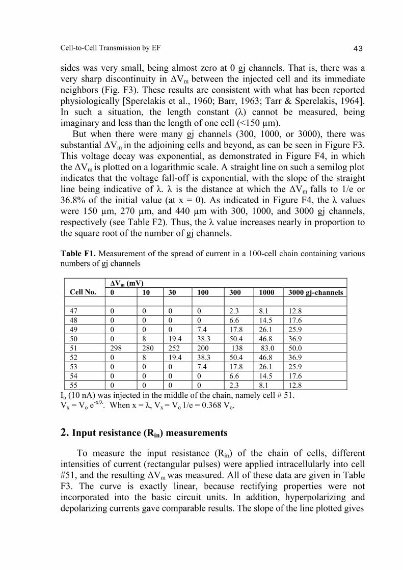
Cell-to-Cell Transmission by EF 43
sides was very small, being almost zero at 0 gj channels. That is, there was a very sharp discontinuity in ΔVm between the injected cell and its immediate neighbors (Fig. F3). These results are consistent with what has been reported physiologically [Sperelakis et al., 1960; Barr, 1963; Tarr & Sperelakis, 1964]. In such a situation, the length constant (λ) cannot be measured, being imaginary and less than the length of one cell (<150 µm). But when there were many gj channels (300, 1000, or 3000), there was substantial ΔVm in the adjoining cells and beyond, as can be seen in Figure F3. This voltage decay was exponential, as demonstrated in Figure F4, in which the ΔVm is plotted on a logarithmic scale. A straight line on such a semilog plot indicates that the voltage fall-off is exponential, with the slope of the straight line being indicative of λ. λ is the distance at which the ΔVm falls to 1/e or 36.8% of the initial value (at x = 0). As indicated in Figure F4, the λ values were 150 µm, 270 µm, and 440 µm with 300, 1000, and 3000 gj channels, respectively (see Table F2). Thus, the λ value increases nearly in proportion to the square root of the number of gj channels. Table F1. Measurement of the spread of current in a 100-cell chain containing various numbers of gj channels
ΔVm (mV) Cell No. 0 10 30 100 300 1000 3000 gj-channels 47 0 0 0 0 2.3 8.1 12.8 48 0 0 0 0 6.6 14.5 17.6 49 0 0 0 7.4 17.8 26.1 25.9 50 0 8 19.4 38.3 50.4 46.8 36.9 51 298 280 252 200 138 83.0 50.0 52 0 8 19.4 38.3 50.4 46.8 36.9 53 0 0 0 7.4 17.8 26.1 25.9 54 0 0 0 0 6.6 14.5 17.6 55 0 0 0 0 2.3 8.1 12.8
Io (10 nA) was injected in the middle of the chain, namely cell # 51. Vx = Vo e-x/λ. When x = λ, Vx = Vo 1/e = 0.368 Vo. 2. Input resistance (Rin) measurements To measure the input resistance (Rin) of the chain of cells, different intensities of current (rectangular pulses) were applied intracellularly into cell #51, and the resulting ΔVm was measured. All of these data are given in Table F3. The curve is exactly linear, because rectifying properties were not incorporated into the basic circuit units. In addition, hyperpolarizing and depolarizing currents gave comparable results. The slope of the line plotted gives
Nicholas Sperelakis & Lakshminarayanan Ramasamy 44
Figure F2. Experiment to measure the spread of current in the linear chain of 100 cells. The myocardial cells were rendered inexcitable by removing their GTABLEs. Depolarizing current pulses (10 nA, 5 ms) were applied intracellularly to cell #51 near the mid-point of the chain, and the resulting membrane voltage changes were recorded from cell #51 and its immediate neighbors (e.g., cells 44-58). The initial voltage was the resting potential of -80 mV. The number of gj channels was varied over a wide range, but the results from only 4 are illustrated in this figure: 0 gj-channels (A), 10 (B), 100 (C), and 1,000 (D). A: With no gj channels, the voltage change in cell #51 was very large (ca 215 mV), whereas there was almost zero voltage change in the contiguous cells (49, 50, 52, 53). B: With 10 gj channels, the ΔVm in cell 51 was ca 200 mV, whereas that in cells on either side (cells 50 & 52) was only about 8 mV. C: With 100 gj channels, the ΔVm in cell 51 was ca 120 mV, that in cells 50 and 52 was ca 40 mV, and that in cells 49 and 53 was ca 8 mV. D: With 1000 gj channels, the ΔVm in cell 51 was ca 84 mV, and those in the contiguous cells were ca 44 mV (cells 50 & 52), ca 26 mV (cells 49 & 53), ca 15 mV (cells 48 & 54), and ca 8 mV (cells 47 & 55).
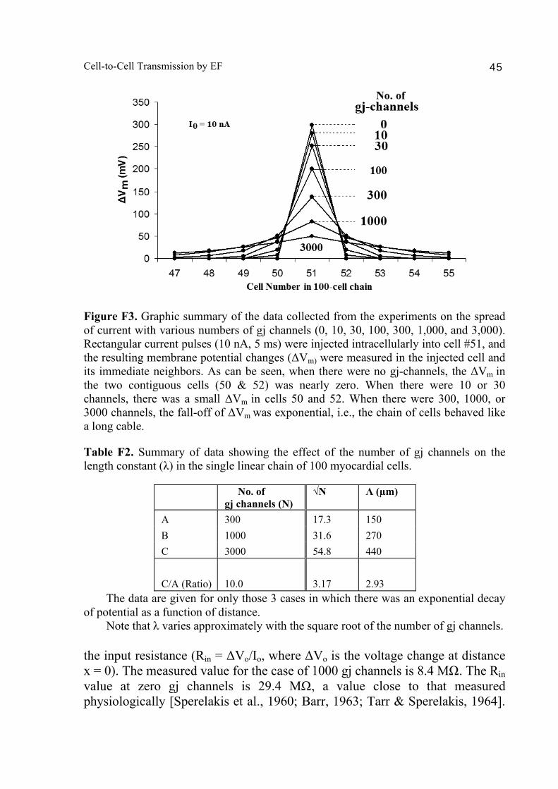
Cell-to-Cell Transmission by EF 45
Figure F3. Graphic summary of the data collected from the experiments on the spread of current with various numbers of gj channels (0, 10, 30, 100, 300, 1,000, and 3,000). Rectangular current pulses (10 nA, 5 ms) were injected intracellularly into cell #51, and the resulting membrane potential changes (ΔVm) were measured in the injected cell and its immediate neighbors. As can be seen, when there were no gj-channels, the ΔVm in the two contiguous cells (50 & 52) was nearly zero. When there were 10 or 30 channels, there was a small ΔVm in cells 50 and 52. When there were 300, 1000, or 3000 channels, the fall-off of ΔVm was exponential, i.e., the chain of cells behaved like a long cable. Table F2. Summary of data showing the effect of the number of gj channels on the length constant (λ) in the single linear chain of 100 myocardial cells.
No. of gj channels (N)
√N Λ (µm)
A 300 17.3 150 B 1000 31.6 270 C 3000 54.8 440 C/A (Ratio)
10.0
3.17
2.93
The data are given for only those 3 cases in which there was an exponential decay of potential as a function of distance.
Note that λ varies approximately with the square root of the number of gj channels. the input resistance (Rin = ΔVo/Io, where ΔVo is the voltage change at distance x = 0). The measured value for the case of 1000 gj channels is 8.4 MΩ. The Rin value at zero gj channels is 29.4 MΩ, a value close to that measured physiologically [Sperelakis et al., 1960; Barr, 1963; Tarr & Sperelakis, 1964].
Nicholas Sperelakis & Lakshminarayanan Ramasamy 46
Table F3 lists the Rin values obtained for all numbers of gj-channels. These values can also be obtained from the ΔVm values measured in cell #51 presented in Figure F3. The equation for calculating Rin is:
Ω=Δ
=0
0
IV
Rin eq. (F3)
where ΔV0 is the voltage change at the site of current injection (x=0) and I0 is the amount of current injected (at x = 0). The equation relating Rin and λ in a cable is:
λ)(21
jini rrR += eq. (F4)
Ω=
Ω+
Ω=Ω cm
cmcm)(
where rm is the internal longitudinal resistance in Ω/cm, and rj is the junctional resistance in Ω/cm. The ½ factor reflects the fact that the injected current spreads in both directions from the point of injection. Since
m
i 0
rλ =r + r
eq. (F5)
2. cm
cmcm
cmcm =Ω
+ΩΩ
=
where rm is the membrane resistance in Ω-cm. Then assuming the external longitudinal resistance r0, to be zero:
mi
jiin r
r
rrR
⎥⎥⎦
⎤
⎢⎢⎣
⎡+=
21 eq. (F6)
=Ω
⎥⎥⎥⎥
⎦
⎤
⎢⎢⎢⎢
⎣
⎡
Ω
Ω
+Ω
=Ω cm
cm
cmcm
.
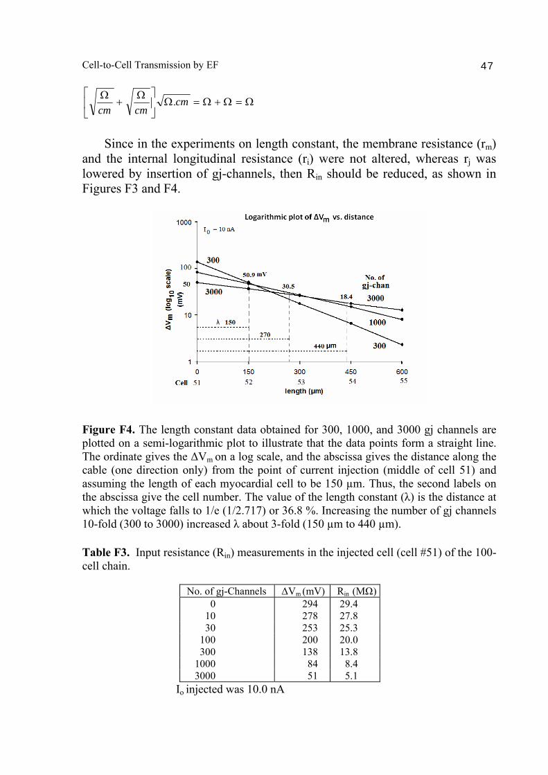
Cell-to-Cell Transmission by EF 47
Ω=Ω+Ω=Ω⎥⎦
⎤⎢⎣
⎡ Ω+
Ω cmcmcm
.
Since in the experiments on length constant, the membrane resistance (rm) and the internal longitudinal resistance (ri) were not altered, whereas rj was lowered by insertion of gj-channels, then Rin should be reduced, as shown in Figures F3 and F4.
Figure F4. The length constant data obtained for 300, 1000, and 3000 gj channels are plotted on a semi-logarithmic plot to illustrate that the data points form a straight line. The ordinate gives the ΔVm on a log scale, and the abscissa gives the distance along the cable (one direction only) from the point of current injection (middle of cell 51) and assuming the length of each myocardial cell to be 150 µm. Thus, the second labels on the abscissa give the cell number. The value of the length constant (λ) is the distance at which the voltage falls to 1/e (1/2.717) or 36.8 %. Increasing the number of gj channels 10-fold (300 to 3000) increased λ about 3-fold (150 µm to 440 µm). Table F3. Input resistance (Rin) measurements in the injected cell (cell #51) of the 100-cell chain.
No. of gj-Channels ΔVm (mV) Rin (MΩ) 0 294 29.4 10 278 27.8 30 253 25.3 100 200 20.0 300 138 13.8 1000 84 8.4 3000 51 5.1
Io injected was 10.0 nA
Nicholas Sperelakis & Lakshminarayanan Ramasamy 48
Bibliography 1. Barr L, "Propagation in vertebrate visceral smooth muscle," J. Theor. Biol., vol. 4,
pp. 73-85, 1. 1963. 2. Cohen S, "Immunocytochemical localization of rH1 sodium channel in adult rat
heart atria and ventricle. Presence in terminal intercalated disks," Circulation, vol. 74, pp. 1071, 1994.
3. Diaz P, Rudy Y and Plonsey R, "Intercalated discs as a cause for discontinuous propagation in cardiac muscle: A theoretical simulation," Ann. Biomed. Eng., vol. 11, pp. 177, 1983.
4. Ge J, Sperelakis N and Ortiz-Zuozaga H, "Simulation of action potential propagation with electronic circuits," Innovation Et Technologie En Biologie Et Médecine, vol. 14, pp. 404-17, 1993.
5. Gutstein D, Morley G, Tamaddon H, D. Vaidya D, M. Schneider M, J. Chen J, K. Chien K, H. Stuhlmann H and G. Fishman G, "Conduction slowing and sudden arrythmic death in mice with cardiac restricted inactivation of connexin43," Circ. Res., vol. 88, pp. 333, 2001.
6. Henriquez C and Plonsey R, "Simulation of propagation along a cylindrical bundle of cardiac tissues. II. Results of simulation," IEEE Trans. Biomed. Eng., vol. 37, pp. 861, 1990.
7. Henriquez C and Plonsey R, "Simulation of propagation along a cylindrical bundle of cardiac tissues. I. Mathematical formulation," IEEE Tans Biomed Eng, vol. 37, pp. 850-11, 1990.
8. Henriquez C, Trayanova N and Plonsey R, "Potential and current distributions in a cylindrical bundle of cardiac muscle," Biophys. J., vol. 53, pp. 907, 1988.
9. Henriquez A, Vogel V, Muller-Borer B, Henriquez C, Weingart R and Cascio W, "Influence of dynamic gap junction resistance on impulse propagation in ventricular myocardium: a computer simulation study," Biophys. J., vol. 81, pp. 2112, 2001.
10. Hogues H, Leon L and Roberge F, "A model of study of electric field interactions between cardiac myocytes," IEEE Tans Biomed Eng, vol. 30, pp. 1232, 1992.
11. Joyner R, Sugiura H and Tan R, "Unidirectional block between isolated rabbit ventricular cells coupled by a variable resistance," Biophys. J., vol. 60, pp. 1038, 1991.
12. Kleber A, Riegger C and Janse M, "Extracellular K+ and H+ shifts in early ischemia: Mechanisms and relation to changes in impulse propagation," J. Mol. Cell. Cardiol., vol. 19, pp. 35, 1987.
13. Koura T, Hara M, Takeuchi S, Ota K, Okada Y, Miyoshi S, Watanabe A, Shiraiwa K, Mitamura H, Kodama I and Ogawa S, "Anisotropic conduction properties in canine atria analyzed by high-resolution optical mapping," Circulation, vol. 105, pp. 2092, 2002.
14. Kucera J, Rohr S and Rudy Y, "Localization of sodium channels in intercalated disks modulates cardiac conduction," Circ. Res., vol. 91, pp. 1176, 2002.
15. Morley G, Vaidya D, Samie F, Lo C, Taffet S, Delmar M and Jalife J, "Characterization of conduction in the ventricles of normal and heterozygous Cx43 knockout mice using optical mapping," J. Cardiovasc. Electrophysiol., vol. 10, pp. 1361, 1999.

Cell-to-Cell Transmission by EF 49
16. Nilsson J.W, Introduction to PSpice® Manual, Electric Circuits: Using ORCad® Release 9.1. , 4th ed. Prentice Hall, 2000.
17. Picone J, Sperelakis N and Mann J, "Expanded model of the electric field: Hypothesis for propagation in cardiac muscle," Math and Computer Modeling, vol. 15, pp. 17, 1991.
18. Poelzing S, Akar F, Baron E and Rosenbaum D, "Heterogeneous connexin43 expression produces electrophysiological heterogeneities across ventricular wall," Am J Physiol: vol. 286, pp. H2001, 2003.
19. Poelzing S and Rosenbaum D, "Altered connexin43 expression produces arrhythmia substrate in heart failure," Am J Physiol: Heart & Circ Physiol, vol. 287, pp. H1762, 2004.
20. Ramasamy L and Sperelakis N, "Action potential repolarization enabled by Ca++ channel deactivation in PSpice simulation of smooth muscle propagation," BioMedical Engineering Online, vol. 4, pp. 71, 2005.
21. Ramasamy L and Sperelakis N, "Gap-junction channels inhibit transverse propagation in cardiac muscle," Biomed Eng Online, vol. 4, pp. 7, 2005.
22. Ramasamy L and Sperelakis N, "Effect of transverse gap-junction channels on transverse propagation in an enlarged PSpice model of cardiac muscle," Theor Biol Med Modeling, vol. 3, pp. 14, 2006a.
23. Ramasamy L and Sperelakis N, "Transverse propagation in an expanded PSpice model for cardiac muscle with gap-junction ion channels," BioMedical Engineering Online, vol. 5, pp. 46, 2006b.
24. Rohr S, "Role of gap junctions in the propagation of the cardiac action potential," Cardiovasc. Res., vol. 62, pp. 309, 2004.
25. Rohr S, Kucera J, Fast V and Kleber A, "Paradoxical improvement of impulse conduction in cardiac tissue by partial cellular uncoupling," Science, vol. 275, pp. 841, 1997.
26. Ruffner A, Sperelakis N and Mann J. E, "Application of the Hodgkin-Huxley equations to an electric field model for interaction between excitable cells," J. Theor. Biol., vol. 87, pp. 129-24, 1980
27. Rudy Y, "The ionic mechanisms of conduction in cardiac tissue," J Electrocardial, vol. 34, pp. 65, 2001.
28. Rudy Y and Quan R, "Effects of the discreet cellular structure on electrical propagation in cardiac tissue," In Electromechanical Activation, Metabolism and Perfusion of the Heart, pp. 61, 1987.
29. Shaw R and Rudy Y, "Ionic mechanisms of propagation in cardiac tissue. Roles of the sodium and L-type calcium currents during reduced excitability and decreased gap junction coupling," Circ. Res., vol. 81, pp. 727, 1997.
30. Spach M and Heidlage J, "The stochastic nature of cardiac propagation at a microscopic level: electrical description of myocardial architecture and its application to conduction," Circ. Res., vol. 76, pp. 366, 1995.
31. Spach M, Miller W, Geselowitz D, Barr R, Kootsey J and Johnson E, "The discontinuous nature of propagation in normal canine cardiac muscle. Evidence for recurrent discontinuity of intracellular resistance that affects the membrane currents," Circ. Res., vol. 48, pp. 39, 1981.
Nicholas Sperelakis & Lakshminarayanan Ramasamy 50
32. Sperelakis N, "Cable properties and propagation of action potentials. Chapt. 18," Cell Physiology Source Book, pp. 245, 1995.
33. Sperelakis N, "Editorial: An electric field mechanism for transmission of excitation between myocardial cells," Circ. Res., vol. 91, pp. 985, 2002.
34. Sperelakis N, "Propagation of action potentials between parallel chains of cardiac muscle cells in PSpice simulation," Can. J. Physiol. Pharmacol., vol. 81, pp. 1, 2003.
35. Sperelakis N and Kalloor B, "Transverse propagation of action potentials between parallel chains of cardiac muscle and smooth muscle cells in PSpice simulations," Biomed Eng Online, vol. 3, 2004.
36. Sperelakis N and Macdonald R, "Ratio of transverse to longitudinal resistivities of isolated cardiac muscle fiber bundles," J. Electrocardiol., vol. 7, pp. 301, 1974.
37. Sperelakis N and Mann J, "Evaluation of electric field changes in the cleft between excitable cells," J. Theor. Biol., vol. 64, pp. 71, 1977.
38. Sperelakis N and McConnell K, "An electric field mechanism for transmission of excitation from cell to cell in cardiac muscle and smooth muscles," In: Research Advances in Biomed. Eng., vol. 2, pp. 39, 2001.
39. Sperelakis N and McConnell K, "Electric field interactions between closely-abutting excitable cells," IEEE-EMB, vol. 21, pp. 77, 2002.
40. Sperelakis N and Murali K, "Combined electric field and gap junctions on propagation of action potentials in cardiac muscle and smooth muscle in PSpice simulation," J. Electrocardiol., vol. 36, pp. 279, 2003a
41. Sperelakis N and Murali K, "Effect of external resistance on propagation of action potentials in cardiac muscle and visceral smooth muscle in PSpice simulation," J Math & Comp Mod., vol. 37, pp. 1443, 2003b.
42. Sperelakis N and Ramasamy L, "Propagation in cardiac muscle and smooth muscle based on electric field transmission at cell junctions: An analysis by PSpice," IEEE-EMB, vol. 21, pp. 130, 2002.
43. Sperelakis N and Ramasamy L, "Gap-junction channels inhibit transverse propagation in cardiac muscle," BioMedical Engineering Online, vol. 4, pp. 7, 2005.
44. Sperelakis N and Ramasamy L, "Propagation velocity profile in a cross-section of a cardiac muscle bundle from PSpice simulation," Theoretical Biology and Medical Modeling, vol. 3, pp. 29, 2006.
45. Sperelakis N, Hoshiko T and Berne R. M, "Nonsyncytial nature of cardiac muscle: membrane resistance of single cells," Am J Physiol, vol. 198, pp. 531-536, 1960.
46. Sperelakis N, Kalloor B and Ramasamy L, "Boundary effects influence velocity of transverse propagation of simulated cardiac action potentials," Theoretical Biology and Medical Modeling, vol. 2, pp. 36, 2005.
47. Sperelakis N, Rollins C and Bryant S. H, "An electronic analog simulation for cardiac arrhythmias and reentry," J. Cardiovasc. Electrophysiol., vol. 1, pp. 294-9, 1990.
48. Spooner P, Joyner R, Jalife J and editors, Discontinuous Conduction in the Heart. Wiley, pp. 569, 1997.
49. Tamaddon H, Vaidya D, Simon A, Paul D, Jalife J and Morley G, "High resolution optical mapping of the right bundle branch in connexin40 knockout mice reveals slow conduction in the specialized conduction system," Circ. Res., vol. 87, pp. 929, 2000.
Cell-to-Cell Transmission by EF 51
50. Tarr M and Sperelakis N, "Weak electronic interaction between contiguous cardiac cells," Am J Physiol, vol. 207, pp. 691-700, 1964.
51. Tront J. G, PSpice for Basic Circuit Analysis, 2nd ed. Boston: McGraw-Hill Higher Education, 2007.
52. Vaidya D, Tamaddon H, Lo C, Taffet S, Delmar M and Morley G, "Null mutation of connexin43 causes slow propagation of ventricular activation in the late stages of mouse embryonic development," Circ. Res., vol. 88, pp. 1196, 2001.
53. Vogel R and Weingart R, "Mathematical model of vertebrate gap junctions derived from electrical measurements on homotypic and heterotypic channels," J. Physiol., vol. 510, pp. 177, 1998.
54. Wang S, Leon L and Roberge F, "Interactions between adjacent fibers in a cardiac muscle bundle," Ann. Biomed. Eng., vol. 24, pp. 662, 1996.
55. Weidmann S, "The diffusion of radiopotassium across intercalated disks of mammalian cardiac muscle," J. Physiol. (Lond.), vol. 187, pp. 322, 1966.
56. Weingart R and Metzger P, "Action potential transfer in cell pairs isolated from adult rat and guinea pig ventricles," Circ. Res., vol. 63, pp. 72, 1988.