propeller characterization - casde.iitb.ac.in · Selecting correct combination of engine and propeller is very crucial step in design of any airworthy vehicle. Whether the output

1

Propeller Characterization

Practical Training Report Submitted by

Kailash Kotwani

Under guidance of Professor S K Sane and Dr. Hemendra Arya

Center for Aerospace System and Design Engineering Department of Aerospace Engineering

Indian Institute of Technology, Bombay August, 2003

2

Abstract

Selecting correct combination of engine and propeller is very crucial step in design of any airworthy vehicle. Whether the output power produced by selected engine propeller combination will be sufficient enough to provide esteemed mission requirements, is the chief question in front of any design engineer. ‘Power vs Velocity’ and ‘Thrust vs Velocity’ characteristics are very important for the design purpose. The information regarding these characteristics is not available in open literature for small propellers and engines used for MAVs. The objective of present study is to establish a measurement system and obtain performance maps for mini propellers and small engines. To reduce the efforts involved and widen the range of analysis, the characteristics are studied using non-dimensional parameters (CP, CT , J etc). Another important aspect is optimizing performance by selecting propeller of best efficiency in the required velocity ranges. These characteristics are determined experimentally using the wind tunnel system built for the MAV development purpose. Different engine-propeller combinations are tested in wind tunnel at different flow velocities. Required plots are generated using data obtained from experiments. Nomenclature A = Area (m2) c = Chord Length (m) CP = Coefficient of Power CT = Coefficient of Thrust CQ = Coefficient of Torque d = Diameter (inch/m) D = Drag (N)/Diameter (inch/m) Eb = Back EMF (V) I = Current Supplied (A) J = Advance Ratio K = DC motor constant L = Lift (N) N = RPM (1/min) n = RPS or Rotational frequency (1/s) P = Power (W) p = pitch (inch) PI = Input Power (W) Po = Output Power (W) PA = Net or Useful power for thrust production (W) Q = Torque (N.m) r = radius (inch/m) Ra = Armature Resistance (Ω) T = Thrust (N) TA = Thrust Available (N)

3

V = Voltage Across motor (V)/Flow Velocity (m/s) VR = Resultant flow Velocity (m/s) V∞ = Translational Velocity Component (Upstream flow velocity) (m/s) Vr = Rotational Velocity Component (m/s) ηx = Efficiency of x ϕ = DC motor flux β = Pitch angle or angle of airfoil with plane of rotation (radian/degree) ω = Rotational Velocity (rad/s) φ = Angle to direction of motion to which VR acts (radian/degree) α = Angle of attack of airfoil (radian/degree) Contents Abstract Nomenclature Contents 1. Introduction 2. Theory and background 3. Operation Limitations

3.1 Motor Operating Limiations 3.2 Propeller Operating Limitations

4. Experiment to determine NO LOAD characteristics of Motor

4.1 Apparatus 4.2 Theory 4.3 Set Up Description and Measurements4.4 Observation: 4.5 Calculations and Analysis 4.6 Conclusions

5. Experiment to predict the shaft power of DC motor

5.1 Apparatus 5.2 Theory 5.3 Experimental Set-up and description 5.4 Observations 5.5 Calculation and Analysis

6. Discussion and Further work References Appendix

A) Motor Specifications B) Observation and Calculation tables C) Matlab Codes

Acknowledgement

4

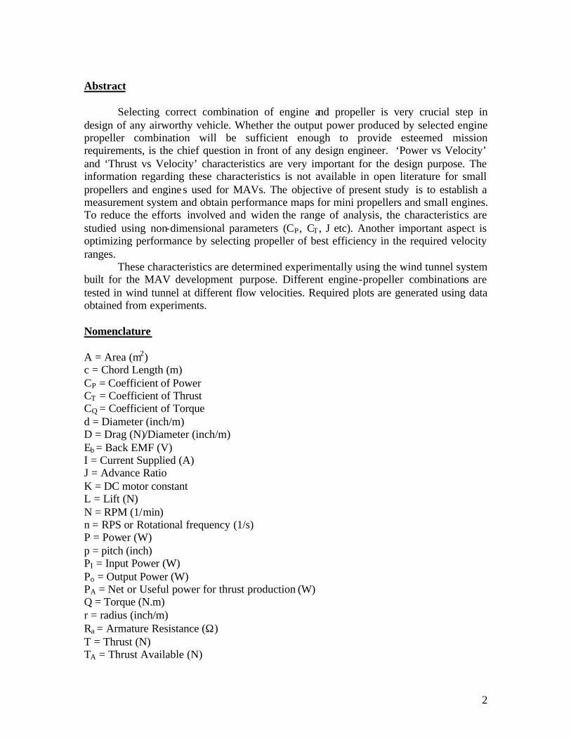
1. Introduction Because of Simplicity, efficiency and cost effectiveness, propeller based IC engines are the best choice as means for thrust production at the first stage of developing a MAV (Mini aerial Vehicle). Thrust and Power generated by a propeller is function of propeller geometry (This include pitch, diameter, airfoil sections at different crossections, weight, no. of blades etc.), flow velocity, RPM and torque applied by the shaft of engine. The MAV being developed will encounter flow velocities in the range of 20 m/s. A wind tunnel system (test section of crossection 1mX1m) has been developed which can generate flow velocities up to 10 m/s (Image 1). In future it will be upgraded to generate velocities in the range of 20 to 25 m/s. So with present system experiments have been conducted upto the velocity of 10 m/s only.

Image 1: Wind Tunnel for experimentation on MAV

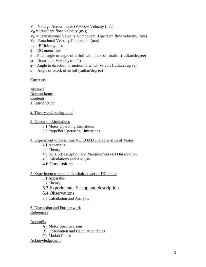
As running an IC engine inside the tunnel involves many complexities e.g. starting trouble, oil in exhaust, variable RPM at constant fuel supply etc. So it was decided to use an electric DC motor for experimentation purpose which is very easy to handle though an IC engine will be used for onboard flights. Here an Astro 15 Cobalt Geared Motor (Model no. p/n 615G) was used for experimentation. Motor is shown in Image 2 and its specifications are given in appendix (A).

5

Image 2: Cobalt Geared DC Motor

There are two methods by which power at the shaft of motor can be estimated

1) Determining No load characteristics then assuming that Back EMF vs RPM characteristics and Mechanical Losses at No Load and Loaded conditions are same.

2) Directly measuring torque at the shaft using torque sensor The task of power measurement using first method has been completed till now (With

an 11X7 Masterscrew glass filled nylon propeller) and is discussed in this section. In this method first armature resistance of motor is measured by short-circuiting it at the supply of very low current and voltage (Armature Resistance is measured at beginning and at the end of experiment because it is sensitive to temperature of motor which varies during the operation). Motor is run under No Load condition (No propeller at the shaft) and input power consumption at different RPM is measured. Hence back EMF and mechanical losses are calculated using theoretical relationship. Again motor is run at loaded condition and Input power consumption is measured at different RPM. Using no load characteristics of back EMF and mechanical losses, shaft power is calculated. This way we obtain Shaft Power vs RPM characteristics. Experiment under Loaded condition is repeated for different flow velocities in wind tunnel and corresponding CP vs J plot is obtained. Shaft Power vs RPM plot at different flow velocities is cross-plotted to obtain Shaft power vs flow velocity plot at different RPM. All these characteristics are analyzed carefully and compared with ones available in literature for larger propeller.

6

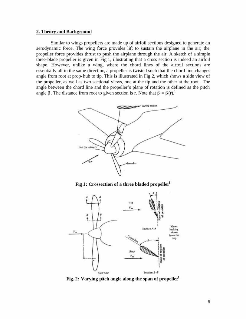
2. Theory and Background Similar to wings propellers are made up of airfoil sections designed to generate an aerodynamic force. The wing force provides lift to sustain the airplane in the air; the propeller force provides thrust to push the airplane through the air. A sketch of a simple three-blade propeller is given in Fig 1, illustrating that a cross section is indeed an airfoil shape. However, unlike a wing, where the chord lines of the airfoil sections are essentially all in the same direction, a propeller is twisted such that the chord line changes angle from root at prop-hub to tip. This is illustrated in Fig 2, which shows a side view of the propeller, as well as two sectional views, one at the tip and the other at the root. The angle between the chord line and the propeller’s plane of rotation is defined as the pitch angle β . The distance from root to given section is r. Note that β = β(r).1

Fig 1: Crossection of a three bladed propeller1

Fig. 2: Varying pitch angle along the span of propeller1

7

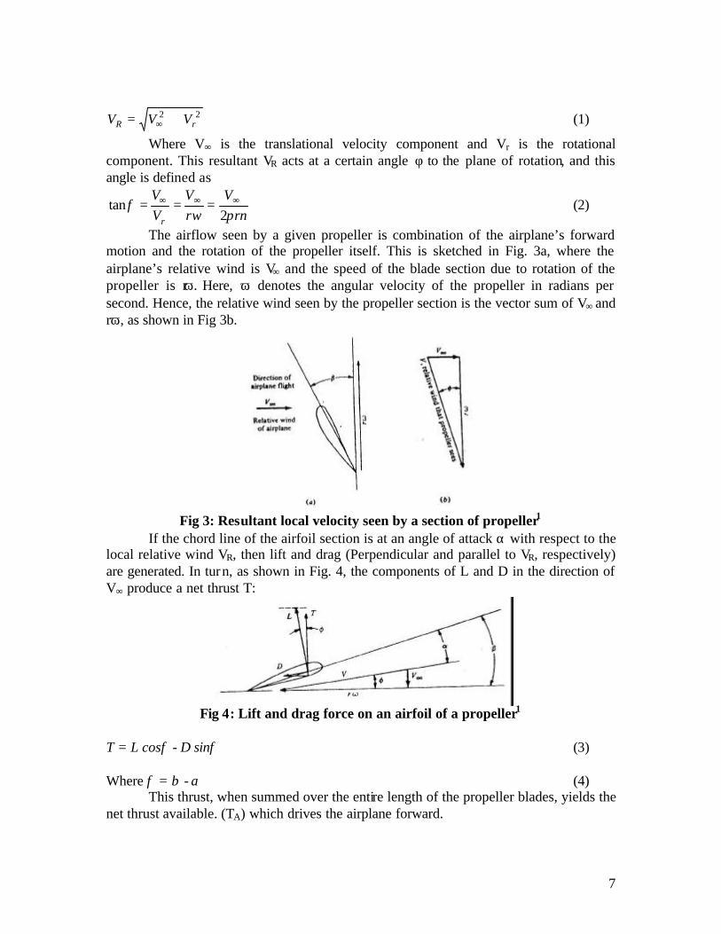
22rR VVV += ∞ (1)

Where V∞ is the translational velocity component and Vr is the rotational component. This resultant VR acts at a certain angle φ to the plane of rotation, and this angle is defined as

rnV

rV

VV

r πωφ

2tan ∞∞∞ === (2)

The airflow seen by a given propeller is combination of the airplane’s forward motion and the rotation of the propeller itself. This is sketched in Fig. 3a, where the airplane’s relative wind is V∞ and the speed of the blade section due to rotation of the propeller is rω. Here, ω denotes the angular velocity of the propeller in radians per second. Hence, the relative wind seen by the propeller section is the vector sum of V∞ and rω, as shown in Fig 3b.

Fig 3: Resultant local velocity seen by a section of propeller1

If the chord line of the airfoil section is at an angle of attack α with respect to the local relative wind VR, then lift and drag (Perpendicular and parallel to VR, respectively) are generated. In turn, as shown in Fig. 4, the components of L and D in the direction of V∞ produce a net thrust T:

Fig 4: Lift and drag force on an airfoil of a propeller1

T = L cosφ - D sinφ (3) Where φ = β - α (4) This thrust, when summed over the entire length of the propeller blades, yields the net thrust available. (TA) which drives the airplane forward.

8

There is one more important parameter, propeller efficiency (η) which is defined as

P

TAAP C

CJ

PVT

PP

? ×=×

== ∞ (5)

Where P is power at the shaft of engine, J is advance ratio, CT is thrust coefficient and CP is power coefficient. The advance ratio J, which is a measure of how far the propeller moves forward through the medium per rotation of the propeller, is defined as

nDV

J ∞= (6)

For a propeller the non dimensional thrust coefficient is defined as

42 DnT

CTρ

= (7)

Similarly, Power coefficient is defined as

53 DnP

CPρ

= (8)

A propeller is nomenclatured in terms of two parameters, pitch and diameter. Pitch is defined as the horizontal distance moved by propeller in one complete rotation at 100 % efficiency and zero slipping. So airfoil at particular section of propeller performs motion in helical direction as shown in Fig. 5. If the helix is unwrapped onto a two dimensional plane, the length p is defined geometrically as

βπ tan.2 rp = (9)

Fig. 5: Measuring Pitch of a propeller4

It should be noted that industry standards are that pitch is measured at 75% of radius that is value of r and β in eqn (9) is what at 75% of radius.

9

3 Operation Limitations 3.1 DC Motor Operating Limitation 1) Voltage, Current and Power Limitations Normal voltage range specified = 8 to 12 Volt (Appendix A) Though 12 volt is not maximum upper limit because the same motor has been used with 12 Nicads battery (Expected performance mapping Appendix A) ∴Maximum Applied voltage = 1.2*12=14.4 Volt. For performance mapping manufacturer has crossed 12 Volt, is confirmed from the fact that with 12 Nicads batteries power consumption was 325 Watt at 24 A current supply ∴ Applied voltage at that time = 325/24=13.54 Volt Another way to obtain maximum voltage across the motor is through maximum continuous current and power specified by manufacturer Maximum Continuous current = 25 A Maximum Continuous power= 400 W Maximum applied voltage = 400/25 = 16 V This analysis shows that it is not unsafe to run motor between 12 to 16 Volt range. One thing should be kept in mind that in high voltage ranges motor should not be run for longer time as motor becomes too hot. Secondly armature resistance is sensible to temperature of motor. Analysis of manufacturer’s specification from three different perspectives is giving three different values of Maximum voltage. This confirms that specification provided by manufacturer is not suitable for engineering analysis and one should develop one’s own safeguards and measuring systems for engineering and research analysis. 2) RPM and Torque Limitations This cobalt motor uses a gear for reducing the final RPM at the shaft. Gear Ratio = 2.38 to 1 (Appendix A) Motor Speed/volt = 1488 rpm/volt Geared motor speed/volt = 652 rpm/volt Lets say maximum applied voltage across the motor = 15 V Geared motor speed = 652*15= 9780 rpm Ungeared motor speed = 22320 rpm This large ungeared speed can be utilized by taking out gear and using motor directly. Even with gear motor provides decent rpm which is in the range of 10000. Similarly, Motor torque/amp = 0.91 in-oz/amp Geared torque/amp = 2.17 in-oz/amp At maximum current = 25 A ∴ Geared torque = 0.91*25=22.75 in-oz Ungeared torque = 2.17*25 = 54.25 in-oz

10

3.2 Propeller operating limitations 1) Noise Considerations

The prop tip speed should not exceed 600 to 650 feet per second (180 to 200 m/s) to keep it within the noise limit (For a master airscrew nylon prop).6

Tip Speed = Vr (ft/s) = rω = 0.00436*RPM*(Diameter in Inches)

DV

RPM r

×=

00436.0 (10)

Lets Say we take limiting propeller tip speed as 600 ft/s For 11X7 master-airscrew propeller, limiting RPM can be calculated Limiting RPM = 600/(0.00436*11) =12510 rpm

2) Mechanical Considerations

One of the differences between wood and glass-filled nylon propellers is that glass- filled nylon props have suggested RPM limits for mechanical considerations. This varies according to Diameter of prop. For a Master Airscrew prop RPM limit recommended by manufacturer is calculated as follows.6

RPM operating limit = 160,000/(Diameter in inches) (11) For a 11X7 prop, RPM operating limit = 160,000/11 = 14,545 rpm Minimum of the above two operating limits will be taken into consideration that

is 12510 rpm.

11

4. Experiment to determine NO LOAD characteristics of Motor The objective of this experiment was 1) To measure the armature resistance of the motor 2) To determine the No Load characteristics of the motor that is obtaining ‘Back EMF vs RPM’ and ‘Mechanical losses vs RPM’ characteristics. The above data will be used to predict the shaft power of DC motor. 4.1 Apparatus

DC Regulated power supply, DM 20 Multimeter, DC Motor, Optical tachometer. 4.2 Theory Voltage eqn of Motor is given as2 V = Eb + I*Ra (12) Multiplying (1) by I V*I = I* Eb+ I2*Ra (13) Where, V*I = Input Power I2*Ra = Electrical losses in armature I* Eb = Mechanical power developed Hence eqn (13) can be interpreted as Input power = Mechanical power developed + electrical losses in armature

Certain percentage of mechanical power developed is required for supplying iron and friction losses in the motor and rest is available as output to drive the shaft of motor Hence one can write eqn as Input power = V*I= mechanical losses + Electrical losses + output (or net available power at the shaft) (14)

Under no load conditions, torque applied at the shaft is zero hence output of motor is zero. That is the total power supplied is used to overcome mechanical and electrical losses only. Output = 0 (under no load conditions) (15) Relationship between speed and back emf of motor is given as2 Eb = N*ϕ/K (16) When RPM is zero back emf is also zero (from (16)). So eqn (13) will become Ra = V/I (17) Using this Ra to calculate back emf for all values of current and voltage. This will enable us to determine characteristic of mechanical losses Vs RPM using eqns (13), (14) and (15). For a constant flux motor back emf is directly proportional to speed of motor (from (16))

12

Hence, Eb α RPM This will provide linear relationship between back emf and RPM, which will be used to evaluate back emf under loaded conditions and hence mechanical power developed.

Fig. 6: Experiment Set up

Image 3: No Load experiment set up

13

4.3 Set Up Description and Measurements: Set up is arranged as shown in Fig. 6 and Image 3. Motor at no load is mounted on rigid stand and connected to power supply. Voltmeter is connected to measure the voltage across the motor. A white patch is marked on shaft of motor of measuring RPM using Tachometer.

Before switching on power supply it is ensured that voltage and current knobs of supply are at zero. Supply is switched on and voltage and current are increased gradually. For measuring Ra, one has to ensure that motor shaft should not rotate and current is brought in the range of 1 amp. After that voltage is measured in steps of 1 volt and readings of current and RPM are noted down. This is done upto 10 volts. At the end of experiment readings are taken again for measuring Ra. Precautions: 1) Select the proper measurement range of voltmeter for accuracy in results. Select

smaller range (i.e. 200 mV or 2 V) for measuring Ra and higher range (20 V) for measuring voltage across the motor.

2) While measuring Ra ensure that shaft of motor is not rotating. Circuit should behave like a short circuit.

3) All electrical devices have transition time for warming up, so after changing any parameter one should wait for sometime to stabilize readings that is steady state.

4) Measure armature resistance at the start and again at the end because of high heating due to long run-time of motor there is enormous difference in both the readings.

4.4 Observation: I set of readings Date: 28th July 2003 Experiment begins at: 11:21 Experiment Ends at: 12:24 Temperature at the start/end: 28.5/29 deg C Pressure at the start/end: 995/996 mbar Humidity at the start/end: 81/80 % Armature Resistance Measurement (Ra):

(Measurements were taken when motor shaft was not rotating.)

Voltage across motor (V) Current Supplied (A) Starting 0.075 1.0

End 0.215 2.0 Table 1: Armature resistance measurement

14

Obs. no.

Voltage Across Motor (V)

Current Supplied (A)

Speed (RPM)

1. 0.98 2.0 476 2. 2.03 2.5 1108 3. 3.01 2.8 1760 4. 4.01 3.7 2455 5. 5.0 4.3 3159 6. 6.0 4.5 3866 7. 7.0 4.8 4587 8. 8.01 5.0 5345 9. 9.01 5.2 6082 10. 10.0 5.2 6770

Table 2: Measuring Voltage, current and speed During this experiment range of voltmeter selected was higher (20 V). Hence it

was decided to repeat the experiment for measuring Ra at lower voltage ranges. Accordingly in the second set of readings, Ra was measured at all possible ranges of voltmeter. II set of readings Date: 2/8/03 Experiment starts at: 11:02 am Ends at: 12.40 pm Temp: 29 oC Pressure: 1001 mbar Humidity: 80% Armature Resistance Measurement (Ra):

(Measurements were taken when motor shaft was not rotating.)

Sr. No. Voltage (V) Current (A) Voltage Range used (V) A) Before starting the experiment

1 0.0775 1 2 V D.C. 2 0.08 1 20 V D.C. 3 0.11 1 200 V D.C. 4 0.0835 1 200 mV D.C.

B) At the end of the experiment 1 0.188 2 2 V D.C. 2 0.235 2 20 V D.C. 3 0.22 1.9 200 V D.C.

Table 3: Armature resistance measurement

Readings obtained at 2 V DC were coming close to the values provided by manufacturer. So it was decided to consider these values only.

15

Obs. no. Voltage Across Motor (V)

Current Supplied (A)

Speed (RPM)

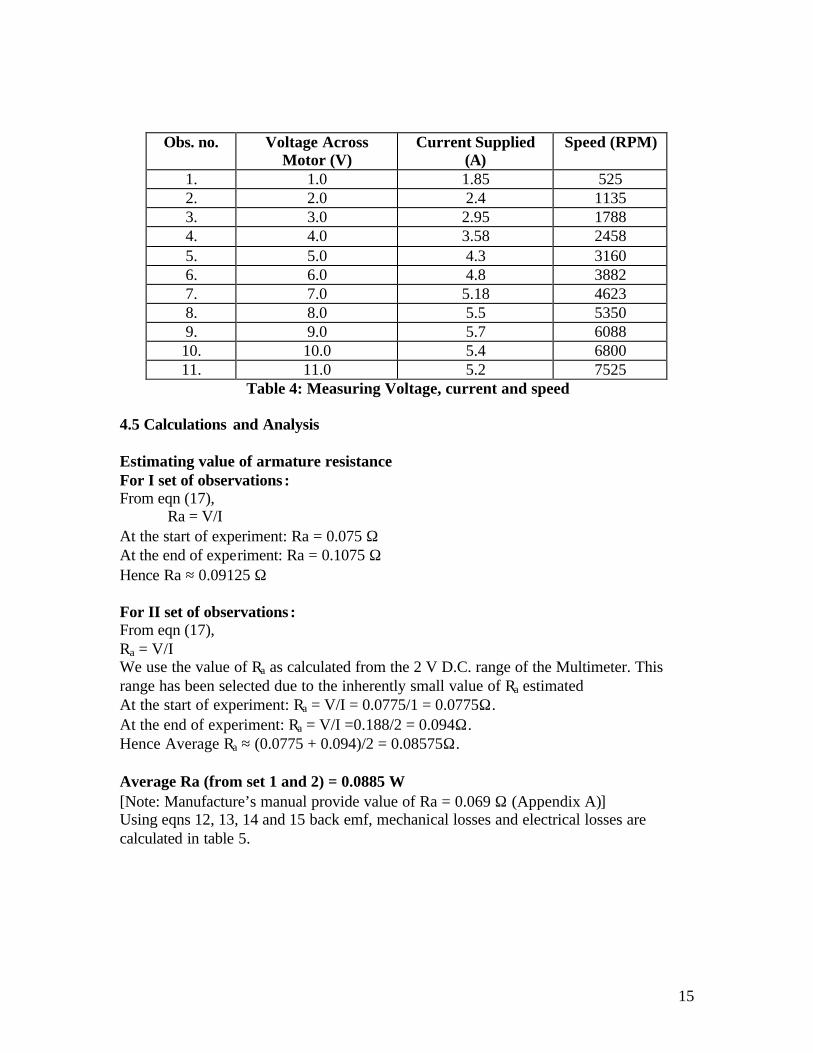
1. 1.0 1.85 525 2. 2.0 2.4 1135 3. 3.0 2.95 1788 4. 4.0 3.58 2458 5. 5.0 4.3 3160 6. 6.0 4.8 3882 7. 7.0 5.18 4623 8. 8.0 5.5 5350 9. 9.0 5.7 6088 10. 10.0 5.4 6800 11. 11.0 5.2 7525

Table 4: Measuring Voltage, current and speed 4.5 Calculations and Analysis Estimating value of armature resistance For I set of observations : From eqn (17),

Ra = V/I At the start of experiment: Ra = 0.075 Ω At the end of experiment: Ra = 0.1075 Ω Hence Ra ≈ 0.09125 Ω For II set of observations : From eqn (17), Ra = V/I We use the value of Ra as calculated from the 2 V D.C. range of the Multimeter. This range has been selected due to the inherently small value of Ra estimated

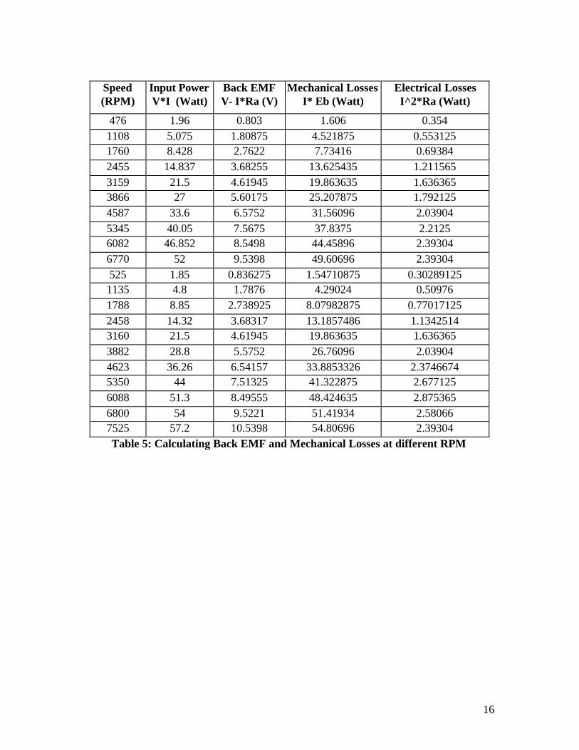
At the start of experiment: Ra = V/I = 0.0775/1 = 0.0775Ω. At the end of experiment: Ra = V/I =0.188/2 = 0.094Ω. Hence Average Ra ≈ (0.0775 + 0.094)/2 = 0.08575Ω. Average Ra (from set 1 and 2) = 0.0885 Ω [Note: Manufacture’s manual provide value of Ra = 0.069 Ω (Appendix A)] Using eqns 12, 13, 14 and 15 back emf, mechanical losses and electrical losses are calculated in table 5.

16

Speed (RPM)

Input Power V*I (Watt)

Back EMF V- I*Ra (V)

Mechanical Losses I* Eb (Watt)

Electrical Losses I^2*Ra (Watt)

476 1.96 0.803 1.606 0.354 1108 5.075 1.80875 4.521875 0.553125 1760 8.428 2.7622 7.73416 0.69384 2455 14.837 3.68255 13.625435 1.211565 3159 21.5 4.61945 19.863635 1.636365 3866 27 5.60175 25.207875 1.792125 4587 33.6 6.5752 31.56096 2.03904 5345 40.05 7.5675 37.8375 2.2125 6082 46.852 8.5498 44.45896 2.39304 6770 52 9.5398 49.60696 2.39304 525 1.85 0.836275 1.54710875 0.30289125 1135 4.8 1.7876 4.29024 0.50976 1788 8.85 2.738925 8.07982875 0.77017125 2458 14.32 3.68317 13.1857486 1.1342514 3160 21.5 4.61945 19.863635 1.636365 3882 28.8 5.5752 26.76096 2.03904 4623 36.26 6.54157 33.8853326 2.3746674 5350 44 7.51325 41.322875 2.677125 6088 51.3 8.49555 48.424635 2.875365 6800 54 9.5221 51.41934 2.58066 7525 57.2 10.5398 54.80696 2.39304 Table 5: Calculating Back EMF and Mechanical Losses at different RPM

17

The values of back emf are plotted against those of motor speeds for both the sets of readings, on the same scale to yield an approximately straight line.

0

2

4

6

8

10

12

0 1000 2000 3000 4000 5000 6000 7000 8000

Motor Speed (RPM)

Bac

k E

MF

(V)

Graph 1: Back EMF vs Motor Speed

Graph 2: Mechanical and Electrical Losses Vs RPM

0

10

20

30

40

50

60

0 1000 2000 3000 4000 5000 6000 7000 8000

Speed (RPM)

Lo

sses

(Wat

t)

Mechanical Losses Electrical Losses

18

4.6 Conclusions 1) Value of Ra = 0.0885 Ω which is closer to the value provided in manufacturer’s

manual (Ra= 0.069Ω). 2) Relationship between back emf and speed is determined as linear experimentally, this matches with theoretical formula. Determined mathematically relationship can be given as Back emf = 0.001366*RPM + 0.2629 (18) 3) Mechanical losses (Iron and friction) are calculated at various speeds and

mathematical relationship between them is obtained Mechanical Losses = -1.5446*E-10*(speed)3 + 1.92*E-6*(speed)2 + 1.5*E-3*(speed) + 0.372 (19) (Matlab code for obtaining eqn (18) and (19) is given in Appendix C (1))

19

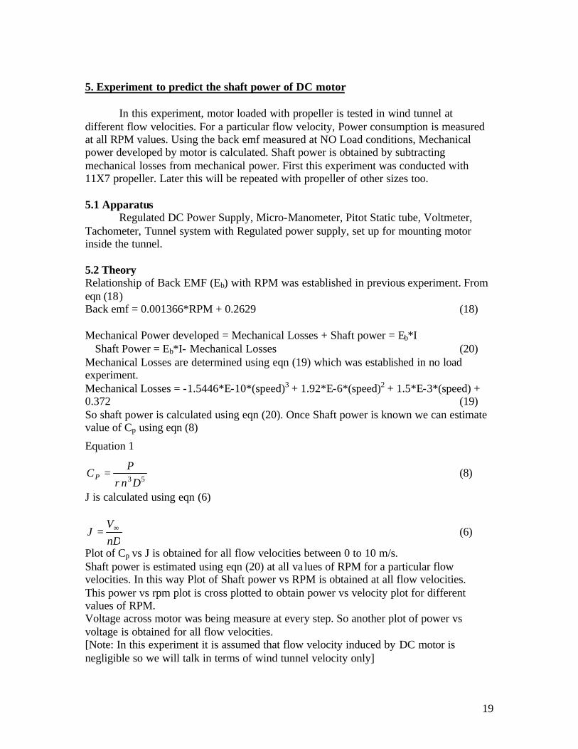
5. Experiment to predict the shaft power of DC motor In this experiment, motor loaded with propeller is tested in wind tunnel at different flow velocities. For a particular flow velocity, Power consumption is measured at all RPM values. Using the back emf measured at NO Load conditions, Mechanical power developed by motor is calculated. Shaft power is obtained by subtracting mechanical losses from mechanical power. First this experiment was conducted with 11X7 propeller. Later this will be repeated with propeller of other sizes too. 5.1 Apparatus Regulated DC Power Supply, Micro-Manometer, Pitot Static tube, Voltmeter, Tachometer, Tunnel system with Regulated power supply, set up for mounting motor inside the tunnel. 5.2 Theory Relationship of Back EMF (Eb) with RPM was established in previous experiment. From eqn (18) Back emf = 0.001366*RPM + 0.2629 (18) Mechanical Power developed = Mechanical Losses + Shaft power = Eb*I ∴Shaft Power = Eb*I- Mechanical Losses (20) Mechanical Losses are determined using eqn (19) which was established in no load experiment. Mechanical Losses = -1.5446*E-10*(speed)3 + 1.92*E-6*(speed)2 + 1.5*E-3*(speed) + 0.372 (19) So shaft power is calculated using eqn (20). Once Shaft power is known we can estimate value of Cp using eqn (8)

Equation 1

53 DnP

CPρ

= (8)

J is calculated using eqn (6)

nDV

J ∞= (6)

Plot of Cp vs J is obtained for all flow velocities between 0 to 10 m/s. Shaft power is estimated using eqn (20) at all va lues of RPM for a particular flow velocities. In this way Plot of Shaft power vs RPM is obtained at all flow velocities. This power vs rpm plot is cross plotted to obtain power vs velocity plot for different values of RPM. Voltage across motor was being measure at every step. So another plot of power vs voltage is obtained for all flow velocities. [Note: In this experiment it is assumed that flow velocity induced by DC motor is negligible so we will talk in terms of wind tunnel velocity only]

20

5.3 Experime ntal Set-up and description Experimental set-up is shown in (Image 4). Motor with a mount is rigidly clamped on a stand and this stand is fixed on the base of tunnel in test-section. Height of stand is such that propeller is at the center of tunnel. A white patch of paint is coated on back side of each blade of propeller. This white patch is for the purpose of reflecting light emanating from optical tachometer fixed at the back of propeller on stand for measuring RPM of propeller. Motor is supplied current from a DC regulated power supply. A voltmeter is connected across motor to measure the voltage. Flow velocity inside the tunnel is controlled using Dimmer stat. A pitot static tube mounted at 78 cm from tunnel inlet is connected to micro-manometer for measuring tunnel flow velocity.

Image 4: Set up inside the tunnel for predicting output power

21

5.4 Observations

First this experiment was conducted when there was no flow inside the tunnel. Later on this experiment was repeated with V=2, 3 …m/s. Observation and Calculation tables for rest of the flow velocities are given in Appendix B. Date : 04/08/03 Obs. No.

Parameter At beginning of the expt.

At end of the experiment

1 Time 16:55 17:20 2 Temperature (ºC) 29 29 3 Pressure (mbar) 1003 1003 4 Relative Humidity 79% 80% 5 Voltage across motor at static

condition (for measuring Ra) (V)

0.104

0.175 6 Current through motor at static

condition (for measuring Ra) (A)

1.5

1.7 Table 6: Measuring Experiment Parameters

Flow Velocity=0 m/s with a 11X7 propeller

Obs. No. Voltage across DC motor

(V)

Current through DC Motor

(A)

2 × Propeller Speed (RPM)

1 1.0 2.1 1062 2 2.0 2.85 2250 3 3.0 3.9 3465 4 4.0 5.0 4750 5 5.0 6.25 5985 6 6.0 7.3 7008 7 7.0 9.0 8464 8 8.0 10.4 9650 9 9.0 11.85 10808 10 10.0 13.35 11900 11 11.0 14.8 12936 12 12.0 16.5 13938

Table 7: Observation table for power consumption and RPM

22

5.5 Calculation and Analysis All the parameters as explained in section 5.2 theory are calculated and their plots are obtained for all flow velocities. (Note: Observation and Calculation tables for velocities other than 0 m/s are given in Appendix B)

Voltage across DC

Motor

Motor RPM

Input Power

Mechanical Losses

Back emf Shaft power

Efficiency of Motor

Cp

1 531 2.1 1.69 0.99 0.39 18.34 0.3053 2 1125 5.7 4.28 1.80 0.85 14.92 0.0709 3 1732.5 11.7 7.95 2.63 2.31 19.73 0.0527 4 2375 20 12.72 3.51 4.82 24.08 0.0427 5 2992.5 31.25 17.95 4.35 9.24 29.57 0.0409 6 3504 43.8 22.60 5.05 14.26 32.56 0.0393 7 4232 63 29.46 6.04 24.93 39.58 0.0390 8 4825 83.2 35.03 6.85 36.25 43.57 0.0383 9 5404 106.65 40.26 7.64 50.33 47.19 0.0378 10 5950 133.5 44.84 8.39 67.17 50.32 0.0378 11 6468 162.8 48.72 9.10 85.93 52.78 0.0377 12 6969 198 51.93 9.78 109.48 55.29 0.0384

Table 8: Calculating Cp and shaft power at zero flow velocity.

For obtaining correct plot of Cp Vs J, all those points which have values of J greater than 0.8 were ignored because J is ratio of forward velocity to rotational velocity at tip of prop. For a MAV in flight Values of RPM are much higher and therefore forward velocity is much lesser than rotational velocity at the tip of prop. Also those first few values of Cp which were obtained at very low power supply giving enormously high values, were ignored.

23

Cp Vs J

-0.02

-0.01

0.00

0.01

0.02

0.03

0.04

0.05

0.06

0.00 0.20 0.40 0.60 0.80 1.00 1.20

J (advancd ratio)

Cp

(po

wer

co

effi

cien

t)

V=2.25 m/s

V=3.19 m/s

V = 3.9 m/s

V = 5.04 m/s

v = 6.36 m/s

V = 7.34 m/s

V = 8.11 m/s

V = 9.18 m/s

V = 9.63 m/s

Graph 3: Cp Vs J plot for velocities 2.25 to 9.63 m/s

Graph 4: Shaft Power vs RPM at different flow velocities

Power vs RPM plot was crossploted using Matlab code (given in Appendix C) to obtain power vs Velocity plot shown in Graph 5.

Shaft Power Vs RPM

-20.00

0.00

20.00

40.00

60.00

80.00

100.00

120.00

140.00

0 1000 2000 3000 4000 5000 6000 7000 8000

Motor Speed (RPM)

Po

wer

Wat

ts

V = 0 m/s

V=2.25 m/s

V=3.19 m/s

V=3.90 m/s

V = 5.04 m/s

V = 6.36 m/s

V = 7.34 m/s

V = 8.11 m/s

V = 9.18 m/s

V = 9.63 m/s

24

Graph 5: Power vs Velocity at different RPM

Graph 6: Power Vs Voltage at different flow Velocities

Plots of Shaft Power v/s Voltage across motor for different observed forward velocities

-20

0

20

40

60

80

100

120

140

0 2 4 6 8 10 12 14

Voltage across motor (Volt)

Sha

ft P

ower

(W

att)

Obs velocity v = 0 m/s

Obs velocity v = 2.25 m/s




obs velocity v = 6.36 m/s



obs velocity v = 9.18 m/s


Power Vs Velocity

-20

0

20

40

60

80

100

120

140

0 2 4 6 8 10 12

Velocity (m/s)

Sha

ft P

ower

(W

att) Power at RPM = 1000

Power at RPM=2000

Power at RPM=3000

Power at RPM=4000

Power at RPM=5000

Power at RPM=6000

Power at RPM = 7000

25

6. Discussion and Further work

1) Upto this point sufficient technical information about the motor and different propellers has been collected and this will serve as an exhaustive matter of reference for further work in future. 2) Motor’s No load characteristics have been determined which helped in predicting power generated at the shaft and obtaining other necessary plots. 3) A typical plot of Cp Vs J is shown in fig. 7 taken from reference no. 4

Fig7. Blade Performance Coefficients4

The plot of Cp Vs J obtained in Graph 3 looks similar to that shown in Fig 7. Even

the maximum value of Cp in both the plot is coming closer to same value of 0.04. This confirms the validity of prediction of shaft power using no load characteristics.

4) From the plot of Power vs RPM (Graph 4), the relationship between power and rpm is

coming cubic which again is in confirmation with physics. 5) Power Vs flow velocity plot (Graph 5) shows that shaft power required to rotate prop

will decrease as flow velocity increases this again confirms physics of system because energy of flow will aid propeller to rotate hence lesser shaft power will be required.

Following Tasks will be completed in future to finish this exercise of power plant measurement.

1) Uninstalled thrust measurement using load cell 2) Uninstalled toque measurement using torque sensors 3) Installed thrust and torque measurements 4) Repeating the whole exercise with different propeller-engine combinations

26

References 1. Anderson, J.D.,”Introduction to Flight”, Mc Graw Hill publishing company, Fourth

Edition, 2000, page no. 595-602. 2. Thareja, B.L., “Introduction to electrical engineering”, S. Chand company and

publisher limited, 1993 3. B B DALY, “Woods Practical Guide to Fan Engineering”, Woods of Colchester

Limited publisher. 4. Von mises, R., “Theory of flight”, Dover Inc., New York,1959 5. http://www.geocities.com/Yosemite/geyser/2126/flyinggadgets.html 6. http://www.masterairscrew.com/techbull.asp(Masterscrew propeller instruction mannual) 7. http://www.astroflight.com (For DC motor instruction manual)

27

Appendix A

Cobalt 15 Geared Motor 7

Cobalt 15 Geared Mtr 2.4 to 1 ratio, 10 to 12 cells, 300W

Astro 15 Cobalt Geared Motor p/n 615G7

Model No. p/n 615G

Name 05 Geared

Gear Ratio 2.38 to 1

Armature Winding 7 turns

Armature Resistance 0.069 ohms

Magnet Type Sm Cobalt

Bearings Ball Bearings

Motor Speed 1488 rpm/volt

Geared Motor Speed 652 rpm/volt

Motor Torque/amp 0.91 in-oz /amp

Geared Torque 2.17 in-oz /amp

Voltage Range 8 to 12 volts

No Load Currrent 2 amps

Maximum Continuous Current 25 amps

Maximum Continuous Power 400 watts

Gear Motor Length 3.3 inches

Motor Diameter 1.3 inches

Motor Shaft Diameter 5/32 inch

Prop Shaft Diameter ¼ inch

Gear Motor Weight 9 oz

Expected Performance of Cobalt 15 Geared Motor7

28

Battery Prop Amps Watts Rpm

10 Nicads 11 x 7 14 amps 168 watts 6,400 rpm




Table 9: Motor specifications and expected performance mapping

Voltage Current Prop Watts RPM 10 5.4 No Load 54 6800 11 5.2 No Load 57.2 7525 10 13.35 11X7 (static flow) 133.5 5950 12 16.5 11X7 (static flow) 198 6969

Table 9A: Performance Results obtained in Lab

29

Appendix B a) Flow velocity: 2.25 m/sec Date: 05/08/03

Obs. No.

Parameter At beginning of the experiment


1 Time 14:30

15:08

2 Temperature (ºC) 28.5 28.5 3 Pressure (mbar) 1002 1002 4 Relative Humidity 81% 81% 5 Voltage across motor at no

load (for measuring Ra) (V)

0.0875 1

6 Current through motor at no load (for measuring Ra) (A)

0.1728

1.8

7 Wattmeter 1 (W) 16 16 8 Wattmeter 2 (W) 13 14 9 Wattmeter 3 (W) 14 14 10 ∆ P (mm of H 2 O) 0.3 0.3 11 Observed Velocity (m/sec) 1.9 2.0 12 Dimmer stat Voltage (V) 72 72

Table 10: Observations: Experiment paramters at V=2.25 m/s

30

Obs. No. Voltage across DC

motor (V)


(A)


1 1.0 2.1 1072 2 2.0 2.9 2260 3 3.0 3.9 3450 4 4.0 5.1 4676 5 5.0 6.4 5940 6 6.0 7.75 7180 7 7.0 9.2 8380 8 8.0 10.6 9560 9 9.0 12.1 10700 10 10.0 13.6 11780 11 11.0 15.2 12800 12 12.0 17.0 13780

Table 11: Observations: Measuring power consumption and propeller speed

Voltage across DC

motor

Propeller Speed(RPM)

Mechanical Losses

Back EMF shaft power

Efficiency of Motor

Cp J

1 536 1.71 1.00 0.38 18.21 0.29 0.92 2 1130 4.30 1.81 0.93 16.11 0.08 0.44 3 1725 7.90 2.62 2.32 19.83 0.05 0.29 4 2338 12.42 3.46 5.20 25.51 0.05 0.21 5 2970 17.75 4.32 9.90 30.93 0.04 0.17 6 3590 23.40 5.17 16.64 35.79 0.04 0.14 7 4190 29.06 5.99 26.01 40.39 0.04 0.12 8 4780 34.62 6.79 37.38 44.08 0.04 0.10 9 5350 39.79 7.57 51.82 47.59 0.04 0.09 10 5890 44.36 8.31 68.64 50.47 0.04 0.08 11 6400 48.25 9.01 88.64 53.01 0.04 0.08 12 6890 51.47 9.67 113.00 55.39 0.04 0.07

Table 12: Calculation: Predicting shaft, Cp and J at V=2.25 m/s

×

31

b) Approach velocity: 3.19 m/sec. Date: 05/08/03

Obs. No.

Parameter At beginning of the exp.


1 Time 15:20 16:00 2 Temperature (ºC) 28.5 28.5 3 Pressure (mbar) 1002 1002 4 Relative Humidity 81% 77% 5 Voltage across motor at no load

(for measuring Ra) (V)

0.1404

0.292 6 Current through motor at no load

(for measur ing Ra) (A)

1.6

1.8 7 Wattmeter 1 (W) 24.2 24.2 8 Wattmeter 2 (W) 22.1 22.1 9 Wattmeter 3 (W) 23 23 10 ∆ P (mm of H 2 O) 0.6 0.6 11 Observed Velocity (m/sec) 3.2 3.2 12 Dimmerstat Voltage (V) 90 90

Table 13: Observation: Measuring Experimental Parameters at V=3.19 m/s


(V)


(A)


1 1.0 2.0 1093 2 2.0 2.6 2270 3 3.0 3.6 3485 4 4.0 4.9 4720 5 5.0 6.5 6000 6 6.0 7.9 7250 7 7.0 9.3 8430 8 8.0 10.9 9610 9 9.0 12.35 10740 10 10.0 14.1 11850 11 11.0 15.85 12900 12 12.0 17.7 13880

Table 14: Observation: Measuring Power Consumption at V=3.19 m/s

32

Voltage Across

the Motor

prop speed

Mechanical Losses

Back EMF

Shaft power

Efficiency of Motor

Cp J

1 546.5 1.74 1.01 0.28 13.76 0.20 1.27 2 1135 4.33 1.81 0.38 7.38 0.03 0.61 3 1742.5 8.01 2.64 1.50 13.90 0.03 0.40 4 2360 12.60 3.49 4.48 22.88 0.04 0.29 5 3000 18.02 4.36 10.33 31.78 0.05 0.23 6 3625 23.73 5.21 17.47 36.85 0.04 0.19 7 4215 29.30 6.02 26.69 41.00 0.04 0.16 8 4805 34.85 6.83 39.56 45.37 0.04 0.14 9 5370 39.96 7.60 53.87 48.47 0.04 0.13 10 5925 44.64 8.36 73.19 51.90 0.04 0.12 11 6450 48.60 9.07 95.22 54.61 0.04 0.11 12 6940 51.77 9.74 120.68 56.82 0.04 0.10

Table 15: Calculations: Shaft power, Cp and J at V=3.19 m/s c) Flow velocity: 3.9 m/sec. Date: 05/08/03

Obs. No.





0.1350


(for measuring Ra) (A)

1.8

1.8 7 Wattmeter 1 (W) 33.5 34 8 Wattmeter 2 (W) 31 32 9 Wattmeter 3 (W) 29 31 10 ∆ P (mm of H 2 O) 0.9 0.9 11 Observed Velocity (m/sec) 3.9 4.0

Table 16: Observations: Measuring experimental parameters

×

33


motor (V)


(A)


1 1.0 2.05 1082 2 2.0 2.5 2300 3 3.0 3.6 3520 4 4.0 5.1 4762 5 5.0 6.65 6000 6 6.0 8.0 7240 7 7.0 9.5 8440 8 8.0 10.9 9600 9 9.0 12.25 10700 10 10.0 13.9 11800 11 11.0 15.5 12800 12 12.0 17.85 13840

Table 17: Observations: Measuring Power Consumption and prop RPM

Voltage Across

DC Motor prop speed

Mechanical Losses

Back EMF

Shaft power

Efficiency of Motor Cp J

1 541 1.72 1.00 0.33 16.07 0.2467 1.57 2 1150 4.41 1.83 0.17 3.48 0.0136 0.74 3 1760 8.13 2.67 1.47 13.59 0.0319 0.48 4 2381 12.77 3.52 5.16 25.30 0.0453 0.36 5 3000 18.02 4.36 10.98 33.03 0.0482 0.28 6 3620 23.68 5.21 17.98 37.46 0.0450 0.24 7 4220 29.35 6.03 27.91 41.98 0.0441 0.20 8 4800 34.80 6.82 39.53 45.34 0.0424 0.18 9 5350 39.79 7.57 52.96 48.03 0.0410 0.16 10 5900 44.44 8.32 71.24 51.25 0.0411 0.14 11 6400 48.25 9.01 91.34 53.57 0.0413 0.13 12 6920 51.65 9.72 121.78 56.85 0.0436 0.12

Table 18: Calculation: Shaft power, Cp and J at V=3.90 m/s

×

34

d) Approach velocity: 5.04 m/sec. Date: 06/08/03 Obs. No.



1 Time 11:20 11:49 2 Temperature (ºC) 28 ºC 28 ºC 3 Pressure (mbar) 998 998 4 Relative Humidity 81% 81% 5 Voltage across motor at no load


0.148



1.75

1.5 7 Wattmeter 1 (W) 43 42.5 8 Wattmeter 2 (W) 41 40.5 9 Wattmeter 3 (W) 40 40 10 ∆ P (mm of H 2 O) 1.5 1.5 11 Observed Velocity (m/sec) 5 5 12 Dimmer stat Voltage (V) 120 120

Table 19: Observation: Measuring Experimental Parameters


(V)


(A)


1 1.0 2.15 1072 2 2.0 2.7 2328 3 3.0 3.6 3560 4 4.0 4.95 4786 5 5.0 6.6 6010 6 6.0 8.0 7250 7 7.0 9.45 8480 8 8.0 10.95 9630 9 9.0 12.5 10740 10 10.0 14.15 11830 11 11.0 15.8 12900 12 12.0 17.6 13880

Table 20: Observations: Measuring power consumption and RPM at V=5.04 m/s

35

Voltage across DC

motor

Prop speed

Mechanical Losses

Back EMF

Shaft power

Efficiency of Motor

Cp J

1 536 1.71 1.00 0.43 20.10 0.33 2.05 2 1164 4.48 1.85 0.52 9.59 0.04 0.95 3 1780 8.27 2.69 1.43 13.23 0.03 0.62 4 2393 12.86 3.53 4.62 23.32 0.04 0.46 5 3005 18.06 4.37 10.77 32.62 0.05 0.37 6 3625 23.73 5.21 17.99 37.48 0.04 0.30 7 4240 29.54 6.05 27.68 41.85 0.04 0.26 8 4815 34.94 6.84 39.96 45.62 0.04 0.23 9 5370 39.96 7.60 55.01 48.90 0.04 0.20 10 5915 44.56 8.34 73.49 51.94 0.04 0.19 11 6450 48.60 9.07 94.76 54.52 0.04 0.17 12 6940 51.77 9.74 119.71 56.68 0.04 0.16

Table 21: Calculations: Shaft power, Cp and J at V=5.04 m/s e) Flow Velocity = 6.36 m/s Date: 08/08/03 Obs. No.





0.088



1.0

1.0 7 Wattmeter 1 (W) 51 50 8 Wattmeter 2 (W) 51 49 9 Wattmeter 3 (W) 48 48 10 ∆ P (mm of H 2 O) 2.4 2.4 11 Observed Velocity (m/sec) 6.0 6.0 12 Dimmer stat Voltage (V) 134 134

Table 22: Observations: Measuring Experimental parameters

×

36


motor (V)


(A)


1 1.0 2.45 1024 2 2.0 2.95 2264 3 3.0 3.7 3510 4 4.0 4.8 4730 5 5.0 6.2 5940 6 6.0 7.95 7140 7 7.0 9.5 8350 8 8.0 10.95 9540 9 9.0 12.5 10700 10 10.0 14 11800 11 11.0 15.7 12840 12 12.0 17.5 13800

Table 23: Observations: Measuring Power consumption and prop RPM

Current through

DC Motor

Prop speed

Mechanical Losses

Back EMF

shaft power

Efficiency of Motor

Cp J

2.45 512 1.63 0.96 0.73 29.87 0.64 2.71 2.95 1132 4.32 1.81 1.02 17.32 0.08 1.23 3.7 1755 8.10 2.66 1.74 15.71 0.04 0.79 4.8 2365 12.64 3.49 4.13 21.51 0.04 0.59 6.2 2970 17.75 4.32 9.03 29.14 0.04 0.47 7.95 3570 23.22 5.14 17.64 36.99 0.05 0.39 9.5 4175 28.92 5.97 27.76 41.74 0.05 0.33

10.95 4770 34.52 6.78 39.70 45.32 0.04 0.29 12.5 5350 39.79 7.57 54.85 48.75 0.04 0.26 14 5900 44.44 8.32 72.07 51.48 0.04 0.24

15.7 6420 48.39 9.03 93.42 54.10 0.04 0.22 17.5 6900 51.53 9.69 118.02 56.20 0.04 0.20

Table 24: Calculations: Shaft power, Cp and J at V= 6.36 m/s

37

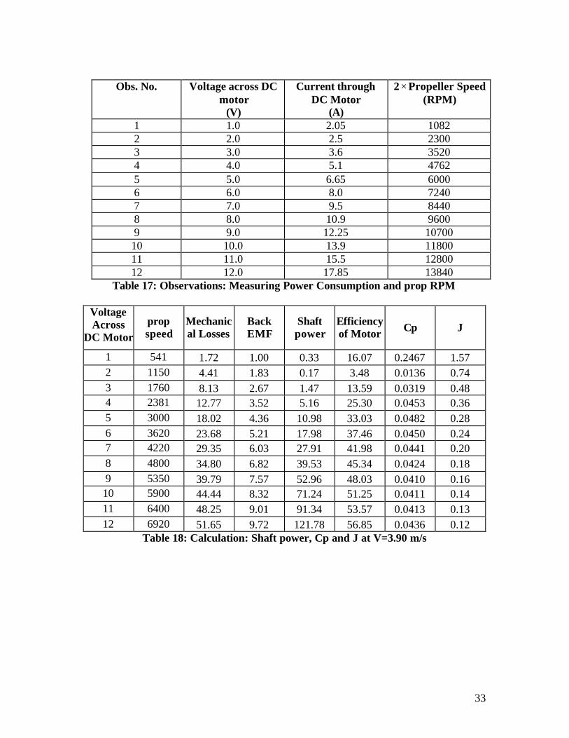
f) Flow Velocity = 7.34 m/s Date: 08/08/03 Obs. No.





0.0774



1.0


Table 25: Observations: Measuring Experimental Parameters


(V)


(A)


1 1.0 2.1 1084 2 2.0 2.5 2326 3 3.0 3.1 3600 4 4.0 4.4 4840 5 5.0 6.15 6080 6 6.0 7.75 7285 7 7.0 9.45 8480 8 8.0 11.0 9650 9 9.0 12.5 10740 10 10.0 14.15 11840 11 11.0 16.0 12890 12 12.0 17.9 13880

Table 26: Observations: Measuring power consumption and prop RPM

38

Voltage

across DC motor

prop speed

Mechanical Losses


Efficiency of Motor

Cp J

1 542 1.73 1.00 0.38 18.04 0.28 2.95 2 1163 4.48 1.85 0.15 2.99 0.01 1.38 3 1800 8.41 2.72 0.03 0.31 0.00 0.89 4 2420 13.08 3.57 2.62 14.88 0.02 0.66 5 3040 18.37 4.42 8.78 28.56 0.04 0.53 6 3642.5 23.89 5.24 16.71 35.93 0.04 0.44 7 4240 29.54 6.05 27.68 41.85 0.04 0.38 8 4825 35.03 6.85 40.36 45.86 0.04 0.33 9 5370 39.96 7.60 55.01 48.90 0.04 0.30 10 5920 44.60 8.35 73.55 51.98 0.04 0.27 11 6445 48.56 9.07 96.50 54.83 0.04 0.25 12 6940 51.77 9.74 122.63 57.09 0.04 0.23

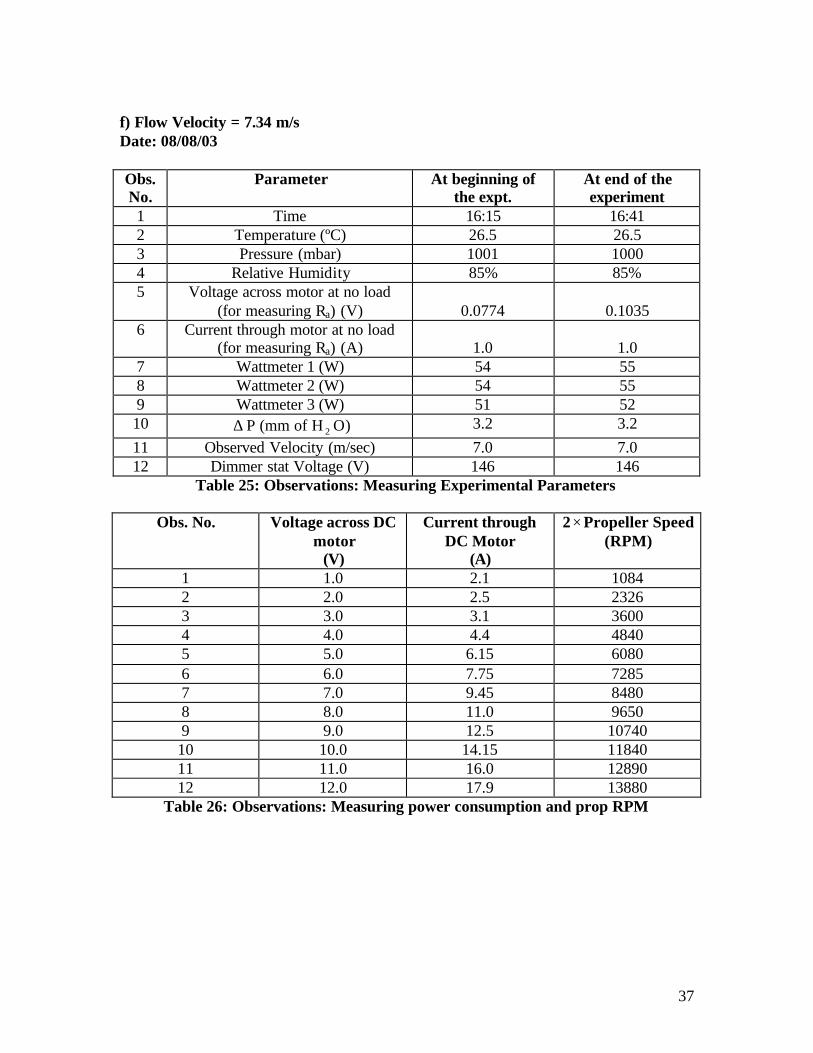
Table 27: Calculations: Shaft Power, Cp and J at V = 7.34 m/s g) Flow Velocity = 8.11 Date: 08/08/03 Obs. No.





0.085



1.0



39


motor (V)


(A)


1 1.0 2.0 1104 2 2.0 2.55 2368 3 3.0 2.95 3650 4 4.0 4.15 4910 5 5.0 5.95 6130 6 6.0 7.7 7350 7 7.0 9.3 8520 8 8.0 10.9 9650 9 9.0 12.6 10800 10 10.0 14.3 11880 11 11.0 16.2 12920 12 12.0 18.0 13880 Table 29: Observations: Measuring power consumption and RPM

Voltage across

DC motor

prop speed

ML Back EMF

shaft powe r

Efficiency of Motor

Cp J

1 552 1.76 1.02 0.27 13.56 0.19 3.20 2 1184 4.59 1.88 0.20 3.96 0.01 1.49 3 1825 8.58 2.76 -0.45 -5.11 -0.01 0.97 4 2455 13.37 3.62 1.64 9.89 0.01 0.72 5 3065 18.60 4.45 7.88 26.49 0.03 0.58 6 3675 24.20 5.28 16.48 35.67 0.04 0.48 7 4260 29.73 6.08 26.84 41.23 0.04 0.42 8 4825 35.03 6.85 39.67 45.50 0.04 0.37 9 5400 40.23 7.64 56.03 49.41 0.04 0.33 10 5940 44.76 8.38 75.03 52.47 0.04 0.30 11 6460 48.67 9.09 98.54 55.30 0.04 0.27 12 6940 51.77 9.74 123.61 57.23 0.04 0.25

Table 30: Calculations: Shaft Power, Cp and J at V= 8.11 m/s

40

h) Flow Velocity = 9.18 m/s Date: 08/08/03 Obs. No.





0.083



1.0




(V)


(A)


1 1.0 2.1 1113 2 2.0 2.7 2396 3 3.0 3.1 3715 4 4.0 4.0 5005 5 5.0 5.7 6255 6 6.0 7.4 7423 7 7.0 9.1 8608 8 8.0 10.9 9720 9 9.0 12.45 10830 10 10.0 13.95 11930 11 11.0 15.8 12980 12 12.0 17.85 13900

Table 32: Observations: Measuring Power Consumption and prop RPM

41

Voltage

across DC motor

Prop speed

Mechanical Losses


Efficiency of Motor

Cp J

1 556.5 1.78 1.02 0.37 17.62 0.25 3.60 2 1198 4.67 1.90 0.46 8.51 0.03 1.67 3 1857.5 8.81 2.80 -0.13 -1.39 0.00 1.08 4 2502.5 13.76 3.68 0.97 6.06 0.01 0.80 5 3127.5 19.16 4.54 6.69 23.49 0.03 0.64 6 3711.5 24.54 5.33 14.92 33.61 0.03 0.54 7 4304 30.14 6.14 25.75 40.43 0.04 0.47 8 4860 35.36 6.90 39.87 45.72 0.04 0.41 9 5415 40.36 7.66 55.01 49.09 0.04 0.37 10 5965 44.96 8.41 72.38 51.88 0.04 0.34 11 6490 48.88 9.13 95.35 54.86 0.04 0.31 12 6950 51.82 9.76 122.33 57.11 0.04 0.29

Table 33: Calculations: Shaft power, Cp and J at V=9.18 m/s

i) Flow Velocity = 9.63 m/s Date: 08/08/03

Obs. No.



1 Time 18:05 18:32 2 Temperature (ºC) 26.5 26.5 3 Pressure (mbar) 999 999 4 Relative Humidity 87 87 5 Voltage across motor at no load


0.08



1.0


Table 34: Observations: Measuring Experimental parameters

42


motor (V)


(A)


1 1.0 2.1 1110 2 2.0 2.65 2386 3 3.0 3.15 3734 4 4.0 3.85 5040 5 5.0 5.55 6280 6 6.0 7.3 7460 7 7.0 9.0 8590 8 8.0 10.75 9735 9 9.0 12.45 10840 10 10.0 14.2 11940 11 11.0 16.0 12940 12 12.0 17.85 13900

Table 35: Observations: Measuring Shaft power and prop RPM

Voltage across DC

motor

Prop speed

Mechanical Losses

Back EMF

shaft power

Efficiency of Motor

Cp J

1 555 1.70 1.02 0.44 21.10 0.31 3.79 2 1193 4.55 1.89 0.47 8.82 0.03 1.76 3 1867 8.74 2.81 0.13 1.34 0.00 1.13 4 2520 13.70 3.71 0.57 3.70 0.00 0.83 5 3140 19.00 4.55 6.27 22.58 0.02 0.67 6 3730 24.38 5.36 14.73 33.64 0.03 0.56 7 4295 29.67 6.13 25.50 40.47 0.04 0.49 8 4867.5 35.00 6.91 39.30 45.70 0.04 0.43 9 5420 39.96 7.67 55.49 49.52 0.04 0.39 10 5970 44.56 8.42 74.98 52.80 0.04 0.35 11 6470 48.33 9.10 97.29 55.28 0.04 0.32 12 6950 51.46 9.76 122.69 57.28 0.04 0.30

Table 36: Calculations : Shaft power, Cp and J at V = 9.36 m/s

43

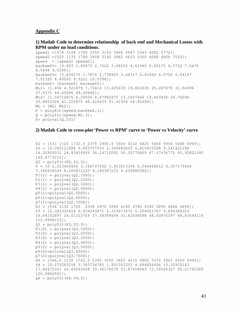
Appendix C 1) Matlab Code to determine relationship of back emf and Mechanical Losses with RPM under no load conditions. speed1 =[476 1108 1760 2455 3159 3866 4587 5345 6082 6770]; speed2 =[525 1135 1788 2458 3160 3882 4623 5350 6088 6800 7525]; speed = [speed1 speed2]; backemf1= [0.803 1.80875 2.7622 3.68255 4.61945 5.60175 6.5752 7.5675 8.5498 9.5398]; backemf2= [0.836275 1.7876 2.738925 3.68317 4.61945 5.5752 6.54157 7.51325 8.49555 9.5221 10.5398]; backemf= [backemf1 backemf2]; ML1= [1.606 4.521875 7.73416 13.625435 19.863635 25.207875 31.56096 37.8375 44.45896 49.60696]; ML2= [1.54710875 4.29024 8.07982875 13.1857486 19.863635 26.76096 33.8853326 41.322875 48.424635 51.41934 54.80696]; ML = [ML1 ML2]; P = polyfit(speed,backemf,1); Q = polyfit(speed,ML,3); R= polyval(Q,531) 2) Matlab Code to cross-plot ‘Power vs RPM’ curve to ‘Power vs Velocity’ curve X2 = [531 1125 1732.5 2375 2992.5 3504 4232 4825 5404 5950 6468 6969]; Y2 = [0.385111588 0.850707533 2.308882603 4.815833598 9.241422298 14.25909031 24.93418906 36.24712091 50.32770609 67.17436772 85.92821245 109.4773216]; Q2 = polyfit(X2,Y2,3); V = [0 2.253405806 3.186797052 3.903013345 5.044668012 6.357179464 7.340638549 8.105871243 9.180387233 9.630880586]; P1(1) = polyval(Q2,1000); P2(1) = polyval(Q2,2000); P3(1) = polyval(Q2,3000); P4(1) = polyval(Q2,4000); p5(1)=polyval(Q2,5000); p6(1)=polyval(Q2,6000); p7(1)=polyval(Q2,7000); X3 = [536 1130 1725 2338 2970 3590 4190 4780 5350 5890 6400 6890]; Y3 = [0.382332824 0.934243871 2.319673572 5.204451707 9.896384323 16.64102897 26.01313759 37.38389699 51.82038098 68.63875297 88.63544116 112.9996123]; Q3 = polyfit(X3,Y3,3); P1(2) = polyval(Q3,1000); P2(2) = polyval(Q3,2000); P3(2) = polyval(Q3,3000); P4(2) = polyval(Q3,4000); p5(2) = polyval(Q3,5000); p6(2)=polyval(Q3,6000); p7(2)=polyval(Q3,7000); X4 = [546.5 1135 1742.5 2360 3000 3625 4215 4805 5370 5925 6450 6940]; Y4 = [0.275283258 0.383734785 1.501352333 4.484856496 10.32920163 17.46675351 26.69245408 39.56170078 53.87458043 73.18566327 95.21765389 120.6842461]; Q4 = polyfit(X4,Y4,3);

44

P1(3) = polyval(Q4,1000); P2(3) = polyval(Q4,2000); P3(3) = polyval(Q4,3000); P4(3) = polyval(Q4,4000); p5(3) = polyval(Q4,5000); p6(3)= polyval(Q4,6000); p7(3)=polyval(Q4,7000); X5 = [541 1150 1760 2381 3000 3620 4220 4800 5350 5900 6400 6920]; Y5 = [0.329375074 0.174241137 1.468123359 5.160188944 10.98333663 17.98033014 27.91407678 39.53365284 52.95603098 71.24057809 91.33703116 121.775865]; Q5 = polyfit(X5,Y5,3); P1(4) = polyval(Q5,1000); P2(4) = polyval(Q5,2000); P3(4) = polyval(Q5,3000); P4(4) = polyval(Q5,4000); p5(4) = polyval(Q5,5000); p6(4)= polyval(Q5,6000); p7(4)=polyval(Q5,7000); X6 = [536 1164 1780 2393 3005 3625 4240 4815 5370 5915 6450 6940]; Y6 = [0.432086624 0.517976713 1.429317758 4.617532275 10.76601841 17.98821851 27.68137638 39.95985194 55.01432843 73.49043 94.76397389 119.7099521]; Q6 = polyfit(X6,Y6,3); P1(5) = polyval(Q6,1000); P2(5) = polyval(Q6,2000); P3(5) = polyval(Q6,3000); P4(5) = polyval(Q6,4000); p5(5)=polyval(Q6,5000); p6(5)=polyval(Q6,6000); p7(5)=polyval(Q6,7000); X7 = [512 1132 1755 2365 2970 3570 4175 4770 5350 5900 6420 6900]; Y7 = [0.731707824 1.022106421 1.743709729 4.128969468 9.032400323 17.64377849 27.75658069 39.70461438 54.84878098 72.07280809 93.42486765 118.0161655]; Q7 = polyfit(X7,Y7,3); P1(6) = polyval(Q7,1000); P2(6) = polyval(Q7,2000); P3(6) = polyval(Q7,3000); P4(6) = polyval(Q7,4000); p5(6)=polyval(Q7,5000); p6(6)=polyval(Q7,6000); p7(6)=polyval(Q7,7000); X8 = [542 1163 1800 2420 3040 3642.5 4240 4825 5370 5920 6445 6940]; Y8 = [0.378887851 0.14932772 0.028784322 2.619389143 8.78337784 16.70609438 27.68137638 40.35943091 55.01432843 73.54693736 96.50455452 122.6328341]; Q8 = polyfit(X8,Y8,3); P1(7) = polyval(Q8,1000); P2(7) = polyval(Q8,2000); P3(7) = polyval(Q8,3000); P4(7) = polyval(Q8,4000); p5(7) = polyval(Q8,5000); p6(7) = polyval(Q8,6000); p7(7) = polyval(Q8,7000); X9 = [552 1184 1825 2455 3065 3675 4260 4825 5400 5940 6460 6940];

45

Y9 = [0.271185775 0.202108448 -0.452495632 1.641359588 7.880408753 16.48156982 26.83777208 39.67404591 56.02743129 75.0299195 98.54458474 123.6071281]; Q9 = polyfit(X9,Y9,3); P1(8) = polyval(Q9,1000); P2(8) = polyval(Q9,2000); P3(8) = polyval(Q9,3000); P4(8) = polyval(Q9,4000); p5(8) = polyval(Q9,5000); p6(8) = polyval(Q9,6000); p7(8)= polyval(Q9,7000); X10 = [556.5 1198 1857.5 2502.5 3127.5 3711.5 4304 4860 5415 5965 6490 6950]; Y10 = [0.370066198 0.459808671 -0.129400758 0.96955156 6.694276971 14.92318331 25.75163058 39.87125821 55.00548826 72.37514697 95.34809061 122.3309858]; Q10 = polyfit(X10,Y10,3); P1(9) = polyval(Q10,1000); P2(9) = polyval(Q10,2000); P3(9) = polyval(Q10,3000); P4(9) = polyval(Q10,4000); p5(9) = polyval(Q10,5000); p6(9) = polyval(Q10,6000); p7(9)=polyval(Q10,7000); X11 = [555 1193 1867 2520 3140 3730 4295 4867.5 5420 5970 6470 6950]; Y11 = [0.443173975 0.467513133 0.126215662 0.569752071 6.266828005 14.73285352 25.49611604 39.30041543 55.49041635 74.97559798 97.28896479 122.6923657]; Q11 = polyfit(X11,Y11,3); P1(10) = polyval(Q11,1000); P2(10) = polyval(Q11,2000); P3(10) = polyval(Q11,3000); P4(10) = polyval(Q11,4000); p5(10) = polyval(Q11,5000); p6(10) = polyval(Q11,6000); p7(10)=polyval(Q11,7000); RPM1 = [V;P1]'; RPM2 = [V;P2]'; RPM3 = [V;P3]'; RPM4 = [V;P4]'; RPM5 = [V;p5]'; RPM6 = [V;p6]'; RPM7 = [V;p7]';

Documents

propeller characterization - casde.iitb.ac.in · Selecting correct combination of engine and propeller is very crucial step in design of any airworthy vehicle. Whether the output