Naval Architecture

Simulating propeller and Propeller-Hull Interaction in OpenFOAM

Master of Science Thesis

Reza Mehdipour

Autumn 2013 Master’s Thesis at Centre for Naval Architecture

Royal Institute of Technology, Stockholm, Sweden

Abstract This is a master’s thesis performed at the Department of Shipping and Marine Technology research group in Hydrodynamics at Chalmers University of Technology and is written for the Center for Naval Architecture at the Royal Institute of Technology, KTH.

In order to meet increased requirements on efficient ship propulsions with low noise level, it is important to consider the complete system with both the hull and the propeller in the simulation. OpenFOAM (Open Field Operation and Manipulation) provides different techniques to simulate a rotating propeller with different physical and computational properties. MRF (The Multiple Reference Frame Model) is, perhaps, the easiest way but is a computationally efficient technique to model a rotating frame of reference. The sliding grid techniques provide the more complex way to simulate the propeller and its surrounding region, rotating and interpolate on interface for transient effects. AMI, Arbitrary Mesh Interface, is a sliding grid implementation which is available in the recent versions of OpenFOAM, introduced in the official releases after v2.1.0. In this study, the main objective is to compare these two techniques, MRF and AMI, to perform the open water characteristics of the propeller with the Reynolds-Averaged Navier-Stokes equation computations (RANS) and study the accuracy in parallel performance and the benefits of each approach. More specifically, a self-propelled ship is simulated to study the interaction between the hull and propeller. In order to simplify and decrease the computational complexity the free surface is not considered. The ship under investigation is a 7000 DWT chemical tanker which is subject of a collaborative R&D project called STREAMLINE, strategic research for innovative marine propulsion concepts. In self-propelled condition, the transient forces on the propeller shall be evaluated. This study investigates the results of the experimental work with advanced CFD for accurate analysis and design of the propulsion. In this thesis, all simulations are conducted by using parallel computing. Therefore, a scalability analysis is studied to find out how to affect the average computational time by using different number of nodes.

Keywords: CFD, OpenFOAM, AMI, MRF, Open Water Characteristics, Self-Propelled Ship, Scalability, Parallel Computing

Preface This thesis is a part of the master degree at KTH, Royal Institute of Technology, and has been carried out at the Department of Shipping and Marine of Chalmers University of Technology.

Acknowledgements I would like to express my sincere gratitude to my supervisor, professor Rickard E Bensow, head of Hydrodynamics Group, for his continuous support throughout the whole project, this work wouldn’t have been possible without him, tack så mycket Rickard. My sincere thanks also go to the PHD students of the Hydrodynamics group department of Shipping and Marine of Chalmers University of Technology particularly Abolfazl Asnaghi, Andreas Feymark and Arash Eslamdoost for taking their time to help me through the project. Goteborg, October2013 Reza Mehdipour

Contents 1 Introduction ............................................................................................................................................... 1

2 Theory ......................................................................................................................................................... 2

2.1 Governing Equations ........................................................................................................................ 2

2.2 Turbulent Flows and Turbulence Modeling .................................................................................. 2

2.3 Turbulent Viscosity Hypothesis ...................................................................................................... 3

2.4 Near Wall Modeling .......................................................................................................................... 4

2.5 Discretization Scheme ...................................................................................................................... 4

2.6 Pressure-Velocity Coupling .............................................................................................................. 5

2.7 Meshing ............................................................................................................................................... 5

2.8 Parallel Computing ............................................................................................................................ 6

2.9 Rotational Motion ............................................................................................................................. 6

2.9.1 The MRF Formulation ............................................................................................................... 7

2.9.2 Sliding Mesh ................................................................................................................................ 8

2.10 Open Water Characteristics ........................................................................................................ 8

3 Softwares ................................................................................................................................................... 9

3.1 OpenFOAM ....................................................................................................................................... 9

3.1.1 OpenFOAM’s Incompressible Solvers .................................................................................. 9

3.2 Mesh Generator ............................................................................................................................... 10

4 Workplan of Model Tests ..................................................................................................................... 12

4.1 STREAMLINE Project .................................................................................................................. 12

4.2 Computational Setup in Open Water Test .................................................................................. 14

4.2.1 Simulation Open Water through AMI Technique ................................................................ 16

4.2.2 Simulation Open Water through MRF Technique ............................................................... 17 4.3 Computational Setup in Self-propelled Test ............................................................................... 17 5 Results and Discussions ........................................................................................................................ 19

5.1 Case I – Open Water Test with Multi Reference Frame, MRF ................................................ 19

5.2 Case II – Open Water Test with Arbitrary Mesh Interface, AMI ............................................ 21 5.3 Open Water Test and Scalability ................................................................................................... 24

5.4 Self-propulsion Test ........................................................................................................................ 25

5.4.1 Case III – Self-propulsion Test with Multi Reference Frame, MRF ................................. 25

5.4.2 Case IV – Self-propulsion Test with AMI ............................................................................ 27 6 Conclusions and Future Work ............................................................................................................. 30

6.1 Conclusion ........................................................................................................................................ 30

6.2 Future Work ..................................................................................................................................... 31

List of Figures 2.1: Coordinate System for Relative Velocity .......................................................................................... 7 3.1: The general structure of the AMI and MRF methods .................................................................. 10 3.2: The geometry and mesh in Ponitwise ............................................................................................. 11 4.1: The simulation domain of the open water test ....................................................................................... 15 4.2: Simulation a propeller by AMI ........................................................................................................ 16 4.3: The geometry of the self-propelled simulation .............................................................................. 18 5.1: Axial velocity distribution for J =1.0 .............................................................................................. 20 5.2: Pressure distribution in suction side for J =0.629. ......................................................................... 20 5.3: Pressure distribution in pressure side for J =0.629................................................................................ 20

5.4: Axial velocity distribution for J =1.0 ............................................................................................... 22 5.5: Pressure distribution in the suction side for J =0.629 ................................................................... 23 5.6: Pressure distribution in the pressure side for J =0.629 ........................................................................ 23

5.7: Propeller reference system adopted for the MRF .......................................................................... 25

5.8: Pressure distribution in the suction side for J =0.629 ................................................................... 26 5.9: Pressure distribution in the pressure side for J =0.629 ................................................................. 26 5.10: Pressure distribution on the hull for J =0.629 .............................................................................. 26 5.11: Pressure distribution on the hull for J =0.629 .............................................................................. 27 5.12: Upstream and downstream wake with the propeller ................................................................... 28 5.13: Longitudinal axial velocity with the propeller .................................................................................... 28

5.14: Upstream and downstream wake generated by the AMI approach ......................................... 28

5.15: Pressure distribution in the pressure side ..................................................................................... 29

5.16: Pressure distribution in the suction side ...................................................................................... 29

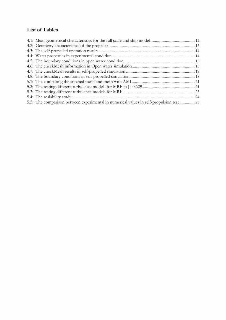
List of Tables 4.1: Main geometrical characteristics for the full scale and ship model ................................................. 12 4.2: Geometry characteristics of the propeller ............................................................................................... 13 4.3: The self-propelled operation results .......................................................................................................... 14 4.4: Water properties in experimental condition ........................................................................................... 14 4.5: The boundary conditions in open water condition .............................................................................. 15 4.6: The checkMesh information in Open water simulation ..................................................................... 15 4.7: The checkMesh results in self-propelled simulation ............................................................................ 18 4.8: The boundary conditions in self-propelled simulation........................................................................ 18 5.1: The comparing the stitched mesh and mesh with AMI ..................................................................... 21 5.2: The testing different turbulence models for MRF in J=0.629 .......................................................... 21 5.3: The testing different turbulence models for MRF ............................................................................... 23 5.4: The scalability study ....................................................................................................................................... 24 5.5: The comparison between experimental in numerical values in self-propulsion test ................. 28

List of Graphs Graph 4.1: Open water characteristics reported from STREAMLINE ................................................ 13 Graph 5.1: The Open water characteristics for the MRF ............................................................................ 19 Graph 5.2: The Open water characteristics for the AMI ............................................................................. 22 Graph 5.3: Scalability analyses .............................................................................................................................. 24

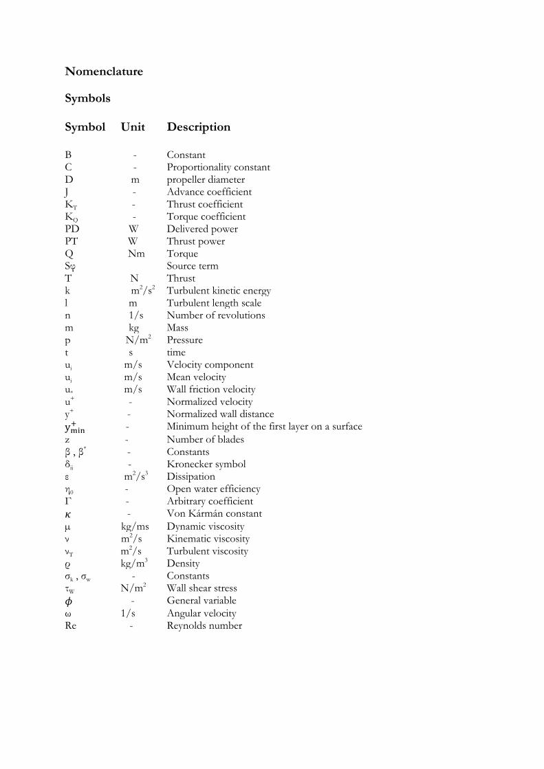
Nomenclature

Symbols Symbol Unit Description

B - Constant C - Proportionality constant D m propeller diameter J - Advance coefficient KT - Thrust coefficient KQ - Torque coefficient PD W Delivered power PT W Thrust power Q Nm Torque Sφ Source term T N Thrust k m2/s2 Turbulent kinetic energy l m Turbulent length scale n 1/s Number of revolutions m kg Mass p N/m2 Pressure

t s time ui m/s Velocity component ui m/s Mean velocity u* m/s Wall friction velocity

u+ - Normalized velocity

y+ - Normalized wall distance

- Minimum height of the first layer on a surface

z - Number of blades β , β* - Constants δij - Kronecker symbol ε m2/s3 Dissipation η0 - Open water efficiency Γ - Arbitrary coefficient

- Von Kármán constant

µ kg/ms Dynamic viscosity ν m2/s Kinematic viscosity νT m2/s Turbulent viscosity ρ kg/m3 Density σk , σw - Constants τW N/m2 Wall shear stress

- General variable

ω 1/s Angular velocity Re - Reynolds number

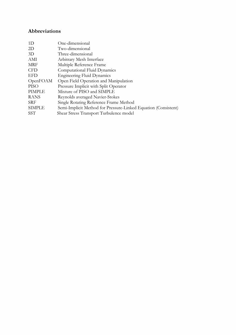
Abbreviations 1D One-dimensional 2D Two-dimensional 3D Three-dimensional AMI Arbitrary Mesh Interface MRF Multiple Reference Frame CFD EFD

Computational Fluid Dynamics Engineering Fluid Dynamics

OpenFOAM Open Field Operation and Manipulation PISO Pressure Implicit with Split Operator PIMPLE Mixture of PISO and SIMPLE RANS Reynolds averaged Navier-Stokes SRF Single Rotating Reference Frame Method SIMPLE Semi-Implicit Method for Pressure-Linked Equation (Consistent) SST Shear Stress Transport Turbulence model

1

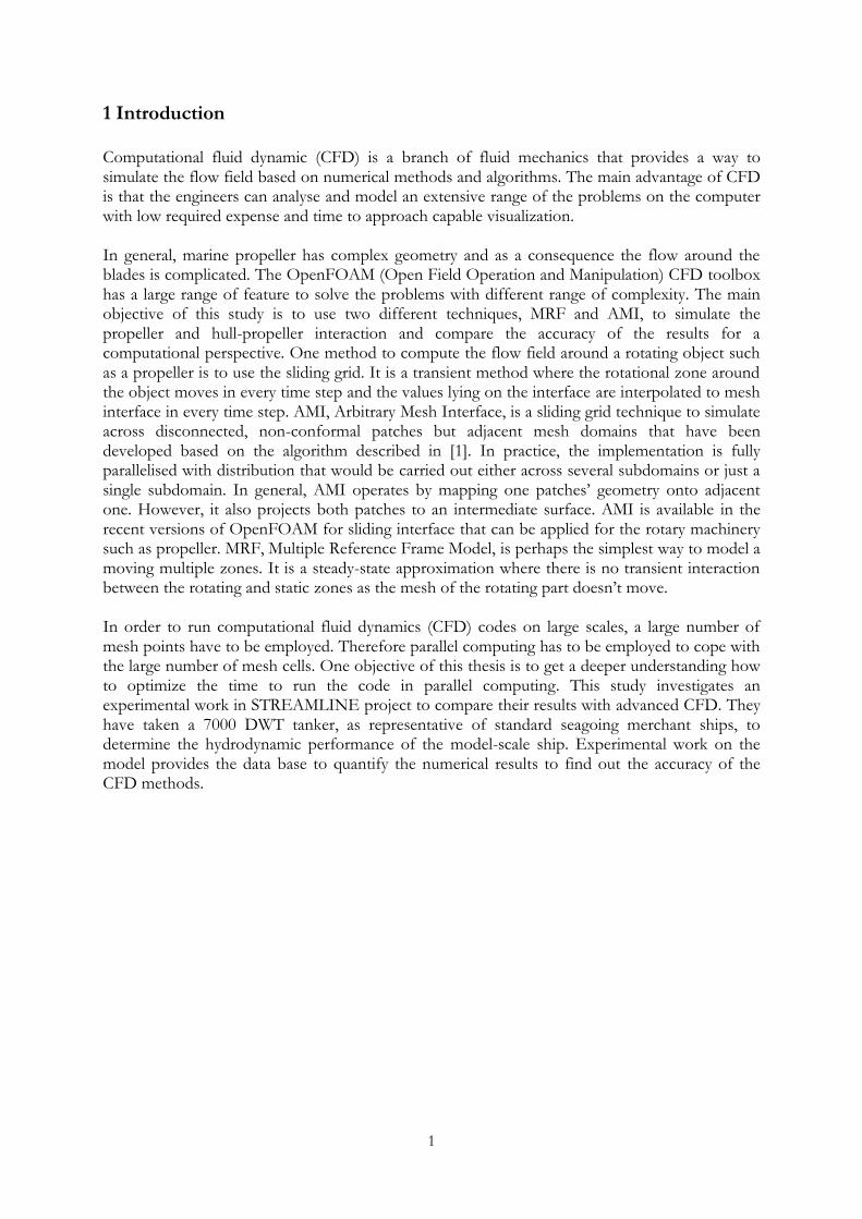
1 Introduction Computational fluid dynamic (CFD) is a branch of fluid mechanics that provides a way to simulate the flow field based on numerical methods and algorithms. The main advantage of CFD is that the engineers can analyse and model an extensive range of the problems on the computer with low required expense and time to approach capable visualization. In general, marine propeller has complex geometry and as a consequence the flow around the blades is complicated. The OpenFOAM (Open Field Operation and Manipulation) CFD toolbox has a large range of feature to solve the problems with different range of complexity. The main objective of this study is to use two different techniques, MRF and AMI, to simulate the propeller and hull-propeller interaction and compare the accuracy of the results for a computational perspective. One method to compute the flow field around a rotating object such as a propeller is to use the sliding grid. It is a transient method where the rotational zone around the object moves in every time step and the values lying on the interface are interpolated to mesh interface in every time step. AMI, Arbitrary Mesh Interface, is a sliding grid technique to simulate across disconnected, non-conformal patches but adjacent mesh domains that have been developed based on the algorithm described in [1]. In practice, the implementation is fully parallelised with distribution that would be carried out either across several subdomains or just a single subdomain. In general, AMI operates by mapping one patches’ geometry onto adjacent one. However, it also projects both patches to an intermediate surface. AMI is available in the recent versions of OpenFOAM for sliding interface that can be applied for the rotary machinery such as propeller. MRF, Multiple Reference Frame Model, is perhaps the simplest way to model a moving multiple zones. It is a steady-state approximation where there is no transient interaction between the rotating and static zones as the mesh of the rotating part doesn’t move. In order to run computational fluid dynamics (CFD) codes on large scales, a large number of mesh points have to be employed. Therefore parallel computing has to be employed to cope with the large number of mesh cells. One objective of this thesis is to get a deeper understanding how to optimize the time to run the code in parallel computing. This study investigates an experimental work in STREAMLINE project to compare their results with advanced CFD. They have taken a 7000 DWT tanker, as representative of standard seagoing merchant ships, to determine the hydrodynamic performance of the model-scale ship. Experimental work on the model provides the data base to quantify the numerical results to find out the accuracy of the CFD methods.

2

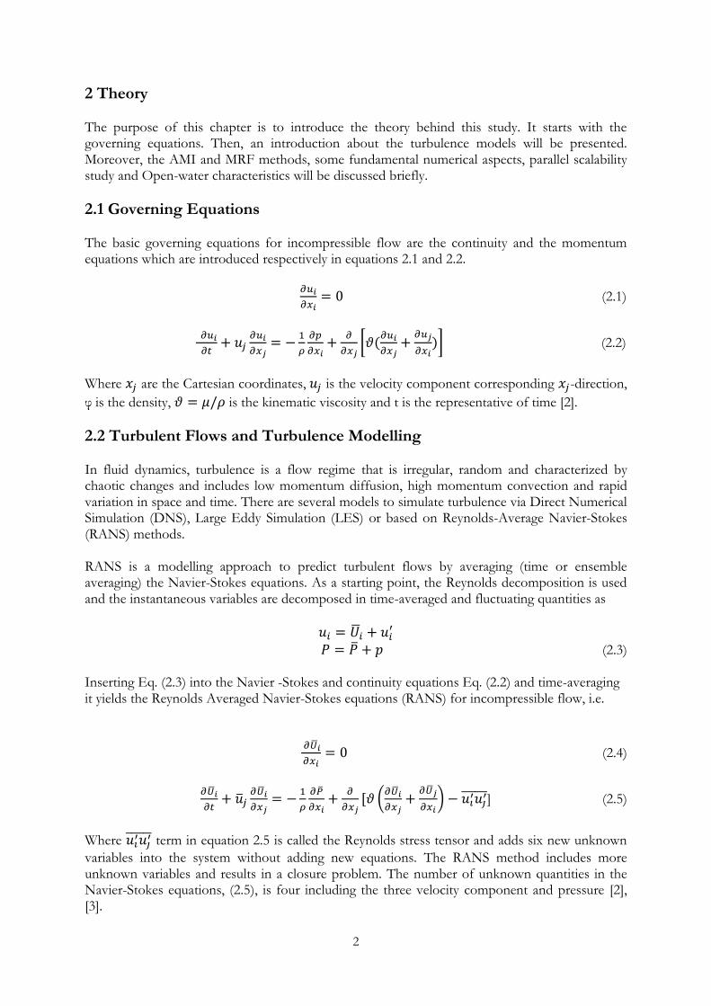
2 Theory The purpose of this chapter is to introduce the theory behind this study. It starts with the governing equations. Then, an introduction about the turbulence models will be presented. Moreover, the AMI and MRF methods, some fundamental numerical aspects, parallel scalability study and Open-water characteristics will be discussed briefly.

2.1 Governing Equations The basic governing equations for incompressible flow are the continuity and the momentum equations which are introduced respectively in equations 2.1 and 2.2.

(2.1)

[

] (2.2)

Where are the Cartesian coordinates, is the velocity component corresponding -direction,

φ is the density, is the kinematic viscosity and t is the representative of time [2].

2.2 Turbulent Flows and Turbulence Modelling

In fluid dynamics, turbulence is a flow regime that is irregular, random and characterized by chaotic changes and includes low momentum diffusion, high momentum convection and rapid variation in space and time. There are several models to simulate turbulence via Direct Numerical Simulation (DNS), Large Eddy Simulation (LES) or based on Reynolds-Average Navier-Stokes (RANS) methods. RANS is a modelling approach to predict turbulent flows by averaging (time or ensemble averaging) the Navier-Stokes equations. As a starting point, the Reynolds decomposition is used and the instantaneous variables are decomposed in time-averaged and fluctuating quantities as

(2.3)

Inserting Eq. (2.3) into the Navier -Stokes and continuity equations Eq. (2.2) and time-averaging it yields the Reynolds Averaged Navier-Stokes equations (RANS) for incompressible flow, i.e.

(2.4)

(

)

] (2.5)

Where

term in equation 2.5 is called the Reynolds stress tensor and adds six new unknown

variables into the system without adding new equations. The RANS method includes more unknown variables and results in a closure problem. The number of unknown quantities in the Navier-Stokes equations, (2.5), is four including the three velocity component and pressure [2], [3].

3

2.3 Turbulent Viscosity Hypothesis In the previous section, we have observed that the number of unknown variables in the Navier-Stokes equations (2.2) is four, the three velocity component and the pressure. The Reynolds

stress tensor,

is a symmetric tensor and contains 6 new unknown variables without adding

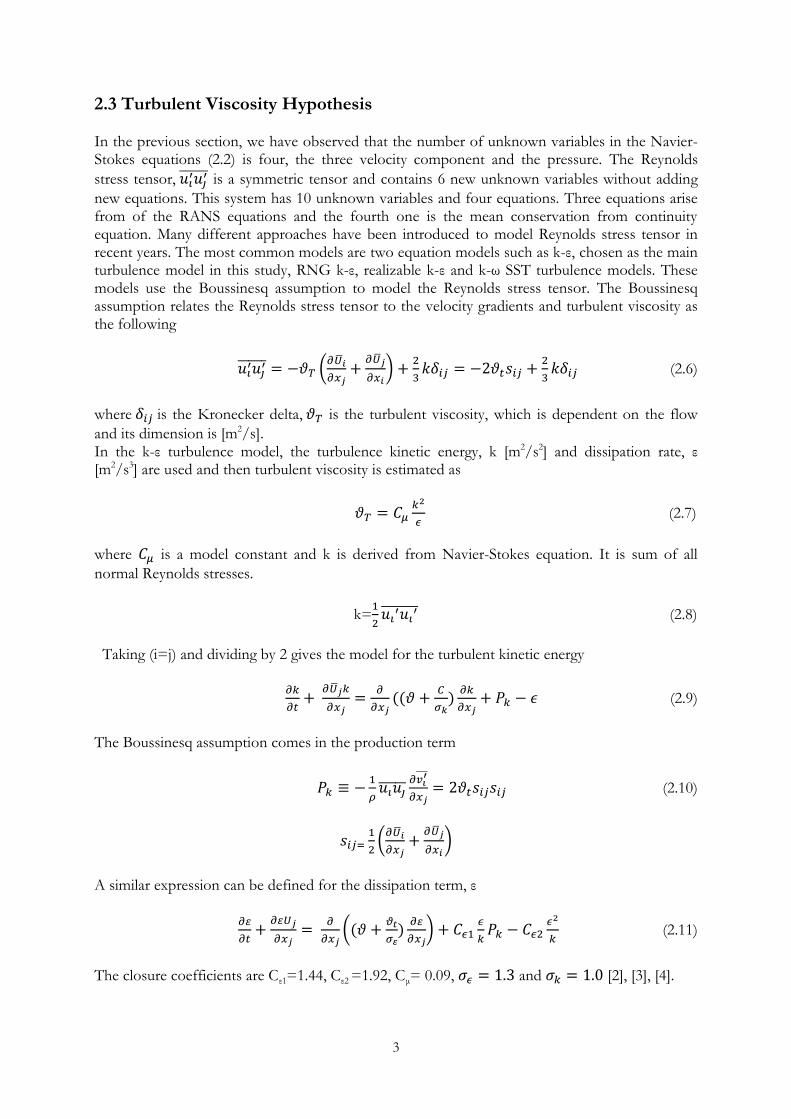
new equations. This system has 10 unknown variables and four equations. Three equations arise from of the RANS equations and the fourth one is the mean conservation from continuity equation. Many different approaches have been introduced to model Reynolds stress tensor in recent years. The most common models are two equation models such as k-ε, chosen as the main turbulence model in this study, RNG k-ε, realizable k-ε and k-ω SST turbulence models. These models use the Boussinesq assumption to model the Reynolds stress tensor. The Boussinesq assumption relates the Reynolds stress tensor to the velocity gradients and turbulent viscosity as the following

(

)

(2.6)

where is the Kronecker delta, is the turbulent viscosity, which is dependent on the flow

and its dimension is [m2/s]. In the k-ε turbulence model, the turbulence kinetic energy, k [m2/s2] and dissipation rate, ε [m2/s3] are used and then turbulent viscosity is estimated as

(2.7)

where is a model constant and k is derived from Navier-Stokes equation. It is sum of all

normal Reynolds stresses.

k=

(2.8)

Taking (i=j) and dividing by 2 gives the model for the turbulent kinetic energy

(2.9)

The Boussinesq assumption comes in the production term

(2.10)

(

)

A similar expression can be defined for the dissipation term, ε

(

)

(2.11)

The closure coefficients are Cε1=1.44, Cε2 =1.92, Cμ= 0.09, and [2], [3], [4].

4

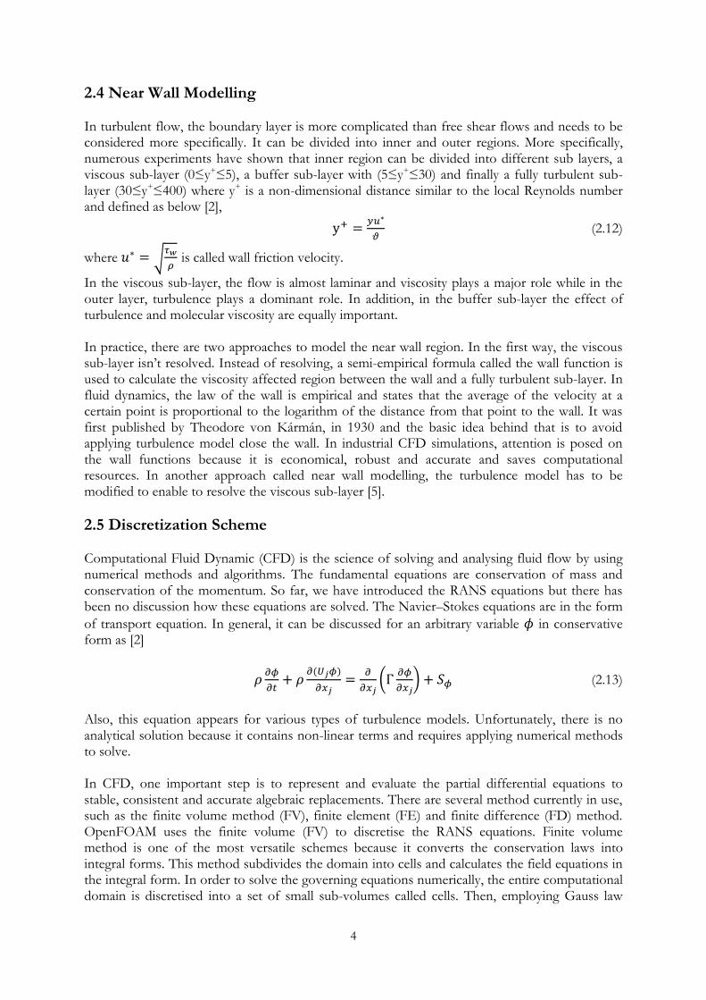
2.4 Near Wall Modelling In turbulent flow, the boundary layer is more complicated than free shear flows and needs to be considered more specifically. It can be divided into inner and outer regions. More specifically, numerous experiments have shown that inner region can be divided into different sub layers, a viscous sub-layer (0≤y+≤5), a buffer sub-layer with (5≤y+≤30) and finally a fully turbulent sub-layer (30≤y+≤400) where y+ is a non-dimensional distance similar to the local Reynolds number and defined as below [2],

(2.12)

where √

is called wall friction velocity.

In the viscous sub-layer, the flow is almost laminar and viscosity plays a major role while in the outer layer, turbulence plays a dominant role. In addition, in the buffer sub-layer the effect of turbulence and molecular viscosity are equally important. In practice, there are two approaches to model the near wall region. In the first way, the viscous sub-layer isn’t resolved. Instead of resolving, a semi-empirical formula called the wall function is used to calculate the viscosity affected region between the wall and a fully turbulent sub-layer. In fluid dynamics, the law of the wall is empirical and states that the average of the velocity at a certain point is proportional to the logarithm of the distance from that point to the wall. It was first published by Theodore von Kármán, in 1930 and the basic idea behind that is to avoid applying turbulence model close the wall. In industrial CFD simulations, attention is posed on the wall functions because it is economical, robust and accurate and saves computational resources. In another approach called near wall modelling, the turbulence model has to be modified to enable to resolve the viscous sub-layer [5].

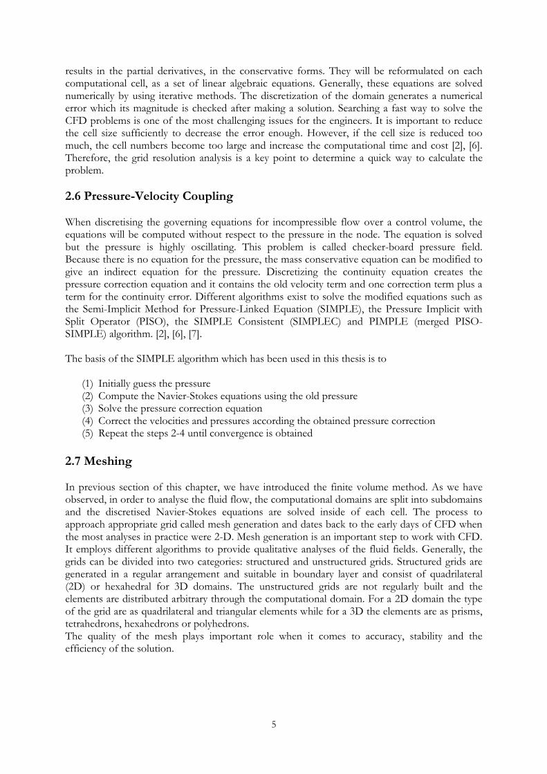
2.5 Discretization Scheme Computational Fluid Dynamic (CFD) is the science of solving and analysing fluid flow by using numerical methods and algorithms. The fundamental equations are conservation of mass and conservation of the momentum. So far, we have introduced the RANS equations but there has been no discussion how these equations are solved. The Navier–Stokes equations are in the form

of transport equation. In general, it can be discussed for an arbitrary variable in conservative form as [2]

(

) (2.13)

Also, this equation appears for various types of turbulence models. Unfortunately, there is no analytical solution because it contains non-linear terms and requires applying numerical methods to solve. In CFD, one important step is to represent and evaluate the partial differential equations to stable, consistent and accurate algebraic replacements. There are several method currently in use, such as the finite volume method (FV), finite element (FE) and finite difference (FD) method. OpenFOAM uses the finite volume (FV) to discretise the RANS equations. Finite volume method is one of the most versatile schemes because it converts the conservation laws into integral forms. This method subdivides the domain into cells and calculates the field equations in the integral form. In order to solve the governing equations numerically, the entire computational domain is discretised into a set of small sub-volumes called cells. Then, employing Gauss law

5

results in the partial derivatives, in the conservative forms. They will be reformulated on each computational cell, as a set of linear algebraic equations. Generally, these equations are solved numerically by using iterative methods. The discretization of the domain generates a numerical error which its magnitude is checked after making a solution. Searching a fast way to solve the CFD problems is one of the most challenging issues for the engineers. It is important to reduce the cell size sufficiently to decrease the error enough. However, if the cell size is reduced too much, the cell numbers become too large and increase the computational time and cost [2], [6]. Therefore, the grid resolution analysis is a key point to determine a quick way to calculate the problem.

2.6 Pressure-Velocity Coupling When discretising the governing equations for incompressible flow over a control volume, the equations will be computed without respect to the pressure in the node. The equation is solved but the pressure is highly oscillating. This problem is called checker-board pressure field. Because there is no equation for the pressure, the mass conservative equation can be modified to give an indirect equation for the pressure. Discretizing the continuity equation creates the pressure correction equation and it contains the old velocity term and one correction term plus a term for the continuity error. Different algorithms exist to solve the modified equations such as the Semi-Implicit Method for Pressure-Linked Equation (SIMPLE), the Pressure Implicit with Split Operator (PISO), the SIMPLE Consistent (SIMPLEC) and PIMPLE (merged PISO-SIMPLE) algorithm. [2], [6], [7]. The basis of the SIMPLE algorithm which has been used in this thesis is to

(1) Initially guess the pressure (2) Compute the Navier-Stokes equations using the old pressure (3) Solve the pressure correction equation (4) Correct the velocities and pressures according the obtained pressure correction (5) Repeat the steps 2-4 until convergence is obtained

2.7 Meshing In previous section of this chapter, we have introduced the finite volume method. As we have observed, in order to analyse the fluid flow, the computational domains are split into subdomains and the discretised Navier-Stokes equations are solved inside of each cell. The process to approach appropriate grid called mesh generation and dates back to the early days of CFD when the most analyses in practice were 2-D. Mesh generation is an important step to work with CFD. It employs different algorithms to provide qualitative analyses of the fluid fields. Generally, the grids can be divided into two categories: structured and unstructured grids. Structured grids are generated in a regular arrangement and suitable in boundary layer and consist of quadrilateral (2D) or hexahedral for 3D domains. The unstructured grids are not regularly built and the elements are distributed arbitrary through the computational domain. For a 2D domain the type of the grid are as quadrilateral and triangular elements while for a 3D the elements are as prisms, tetrahedrons, hexahedrons or polyhedrons. The quality of the mesh plays important role when it comes to accuracy, stability and the efficiency of the solution.

6

Below, different aspects of quality are introduced briefly [6]: Non-Orthogonaility errors concerns on the angle between the face normal and the vector between the cell midpoint and the face. In order to approach well-converged solutions, we avoid high non-orthogonal cells. Aspect ratio is related to the squareness of the cells, for instance for a cube the aspect ratio equals to one. High aspect ratio implies that the cells are stretched in one direction. One reason to approach poor results is that the cells with high aspects ratio are not aligned with the local flow structure. High skewness usually relates with small faces and is defined as the nearest of the intersection between the face node and the vector from the center node and the neighbourhood node. It reduces the quality of the solution but might be unavoided when the geometry is complex like a propeller.

2.8 Parallel Computing In order to compute CFD problems with complex geometries and fluid flows a large number of cells have to be employed. Therefore parallel computing is an appropriate choice to cope with this problem. Developing computer clusters with high performance has become significant means to improve efficiency. Computer clusters consists of a set of connected computers that work together and they can be considered as a single system. They are desired to compute large complex CFD problems with more computing reliability and performance. One challenging issue in industrial CFD is to distribute the cells among the multi-grids to approach a good performance on parallel computing. The time per iteration reduces by increasing number of processors, however the efficiency of the parallel performance is dependent the meshing and the processors. Normally, CFD simulation is affected by the quality of the mesh. A high-quality mesh makes the computational performance quicker and approaches to the more accurate results. One main issue in this thesis is to predict how to affect the average computational time with employing different number of processors. Consequently, it helps us to optimize the parallel computing that leads save time and energy [8], [9]. In this thesis, all simulations will be conducted by using parallel computing since the cases are too large.

2.9 Rotational Motion There are a variety of engineering problems involving rotational parts. Consider a rotating propeller behind a ship, to compute the interaction between a propeller and hull the sliding interface is required to provide the exchange of information between non-matching parts of the cells. Another solution is to use reference frames. A variety of problems can be solved with this capability such as, impeller in mixing tanks, axial fans or cooling ducts. When there are no stators or baffles, the simulation can be performed in a domain that moves with rotating part and the flow is steady relative to the rotating frame that makes the calculation simple. On the other hand, if the stators or baffles are added in closely adjacent, the solution is more complex and the stator-rotor interaction will be important. Therefore, it is not feasible to perform the computation as steady by choosing a computational domain which rotates with the rotor or impeller. There are different approaches to solve these kinds of problems. The multiple reference frame model or MRF in which the flow is assumed steady and cell zones move at different rotational/translational speeds. The cells in the rotational domain are static and their positions don’t have to be recalculated in each time step. It is the model of choice where the rotor-stator interaction is relatively weak or an approximation is required. It gives acceptable time-averaged

7

consequences for many engineering problems. Furthermore, this approach is appropriate when the flow at the boundary between the zones are assumes approximately uniform. We can also model a problem with MRF to compute a flow field that can be used as initial condition of a transient sliding mesh calculation [10].

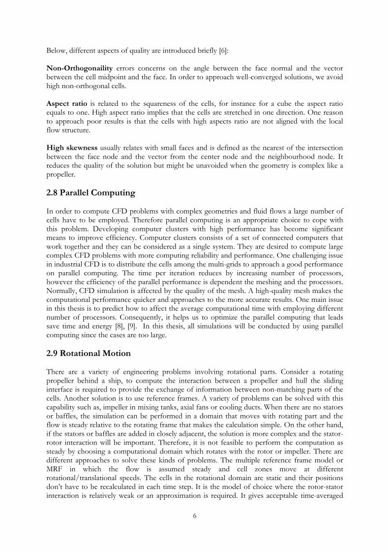
2.9.1 The MRF Formulation In MRF implementation, the computational domain is divided into two subdomains that can be assumed as rotating or translating according to the initial frame. The governing equations in each sub-domain are obtained on the sub-domain’s reference frame. When the relative velocity is used, the position vector relative to the origin of the zone rotation axis is defined as

(2.14)

Let and be the position of the absolute Cartesian coordinate system and the origin of the zone rotation axis respectively.

Figure 2.1: Coordinate System for Relative Velocity [10]

To obtain the absolute velocity, the relative velocity in the moving reference frame can be augmented to the velocity in the rotational zone using the following equation:

(2.15)

Where is the velocity in the absolute inertial reference frame, is defined as the velocity in the

relative reference frame and is the translational velocity of non-inertial reference frame. Using these definitions into Navier-Stokes equations gives the governing equations for the inertial reference frame.

(2.16)

(2.17) Calculating the governing equations for the rotating reference frames results

(2.18)

(2.19)

8

Using the relative formulation respect to the rotating reference of frame derives the governing equations for the frame.

(2.20)

(2.21) Where the second term is the additional Coriolis and the third one is defined as centripetal acceleration [10].

2.9.2 Sliding Mesh The sliding mesh is a computational unsteady technique to model the CFD problems. It is performed, as the interaction between stator and rotor is strong and more accurate computation is desired. The idea behind the sliding mesh is too complex and is not covered in this thesis. AMI is a sliding mesh technique where the rotational zone around the object moves in every time step and the values lying on the interface are interpolated to update the mesh in every time step. It enables to simulate across disconnected, non-conformal patches but adjacent mesh domains that have been developed based on the algorithm described in [1]. In practice, the implementation is fully parallelised with distribution that would be carried out either across several subdomains or just a single subdomain. In general, AMI operates by mapping one patches’ geometry onto adjacent one. However, it also projects both patches to an intermediate surface. AMI is available in the recent versions of OpenFOAM for sliding interface that can be applied for the rotary machinery such as propeller.

2.10 Open Water Characteristics Propeller tests in open water are commonly used to derive the graph of hydrodynamic performance of the propeller while it is acting in different working conditions. The test is conducted in uniform flow in a towing tank or a cavitation tunnel. During the test the revolution is often assumed constant whereas the advance velocity VA varies. Regarding the following expressions, thrust and torque acting on the blades are measured to derive the hydrodynamic coefficients of the propeller over the advanced coefficient (J) [13].

(2.22)

(2.23)

where is the density of the water in the towing tank or cavitation tunnel, n is the revolution in rps and D is diameter of the propeller in [m]. Furthermore, the efficiency of the propeller is introduced as the ratio of the thrust power PT=TVA and delivered power defined as PD=2πnQ.

(2.23)

Comparison between the open-water characteristics and numerical results leads to estimate how accurate the numerical methods are. In this thesis, the open water graph is provided by the STREAMLINE project that will be introduced in next chapter.

9

3 Softwares This chapter includes an overview of the source software which has been employed in this work. OpenFOAM as the CFD source code, its solvers and numerical schemes will be discussed. It also gives a brief introduction about Pointwise that has been used as the mesh generator in this study.

3.1 OpenFOAM This study uses OpenFOAM OpenSource CFD tool to compute the incompressible flow field around the propeller and the propeller-hull interaction in the self-propulsion condition. OpenFOAM (Open source Field Operation and Manipulation) is a free, open source computational fluid dynamic (CFD) software package that provides different solvers, libraries and different utilities for various CFD problems released by OpenCFD. The initial purpose of OpenFOAM was to develop a more robust and flexible simulation platform than FORTRAN. C++ as a programming language was a good choice because its highest modularity and being object oriented. Today, OpenFOAM is known as a powerful, flexible, cost effective tool to model the CFD problems. In addition, it is an open source tool that makes it more attractive in engineering applications. The present work uses the OpenFOAM-2.1x released in 2011 as the CFD code. It should be noted that further information can be found either in the OpenFOAM User Guide or on the OpenFOAM homepage [12], [14].

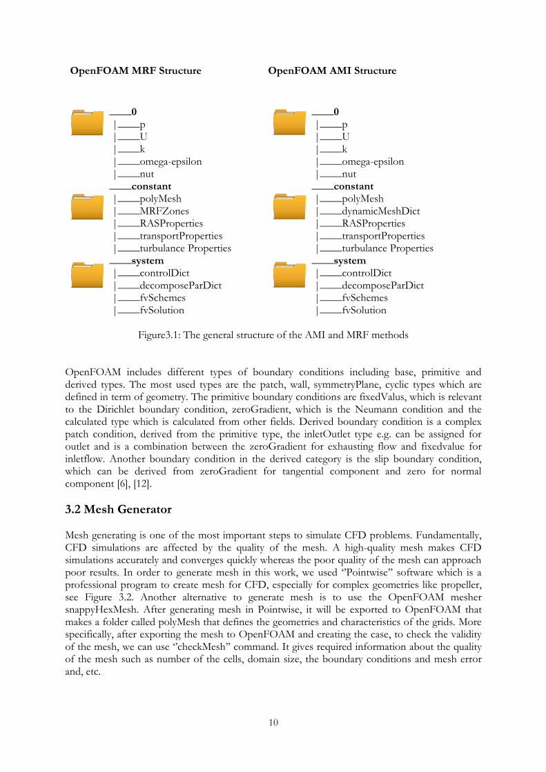
3.1.1 OpenFOAM’s Incompressible Solvers Today, OpenFOAM is used not only for CFD but also for other areas such as stress analyses, finance and electromagnetics. Nevertheless, it has been found mainly for CFD affairs thus a set of various solvers are available depending on the CFD problems. In order to analyse the CFD incompressible problems, different solvers have been developed following the nature of the problem such as icoFoam, channelFoam, MRFSimpleFoam and pimpleDyMFoam (DyM is abbreviation of Dynamic). In this study, MRFSimpleFoam and pimpleDyMFoam are used respectively for MRF and AMI techniques. MRFSimpleFoam is a steady-state solver for incompressible fluids with MRF regions while pimpleDyMFoam is an unsteady solver for incompressible fluids on a moving mesh using the PIMPLE (merged PISO-SIMPLE) algorithm. Normally, OpenFOAM’s solvers have a typical structure which consists of different subdomains. In the time 0 subdirectory boundary and initial condition are defined and when running the case, solver creates corresponding time subdirectories for each time solution solved. The sub-directory constant provides information about mesh and employed turbulence model. The sub-directory system includes the computational schemes and solutions parameters. The fvSchemes dictionary in the system folder describes the numerical schemes for the equations terms. Also, fvSolution in the system contains a set of subdirectories that solver needs during runtime. It specifies the equation solvers, tolerance and algorithms. One important sub-directory in the system is cotroldict that determines the time steps, maximum courant number, the required functions to measure the forces on the blades, start time, end time and writing time of the output files, etc. Finally, the computational results can be exported for a post-processing program, for instance ParaView, to visualize the simulation. Figure 3.1 shows the templates of the OpenFOAM’s structure for to the AMI and MRF solvers.

10

OpenFOAM MRF Structure OpenFOAM AMI Structure

____0 |____p |____U |____k |____omega-epsilon |____nut ____constant |____polyMesh |____MRFZones |____RASProperties |____transportProperties |____turbulance Properties ____system |____controlDict |____decomposeParDict |____fvSchemes |____fvSolution

____0 |____p |____U |____k |____omega-epsilon |____nut ____constant |____polyMesh |____dynamicMeshDict |____RASProperties |____transportProperties |____turbulance Properties ____system |____controlDict |____decomposeParDict |____fvSchemes |____fvSolution

Figure3.1: The general structure of the AMI and MRF methods

OpenFOAM includes different types of boundary conditions including base, primitive and derived types. The most used types are the patch, wall, symmetryPlane, cyclic types which are defined in term of geometry. The primitive boundary conditions are fixedValus, which is relevant to the Dirichlet boundary condition, zeroGradient, which is the Neumann condition and the calculated type which is calculated from other fields. Derived boundary condition is a complex patch condition, derived from the primitive type, the inletOutlet type e.g. can be assigned for outlet and is a combination between the zeroGradient for exhausting flow and fixedvalue for inletflow. Another boundary condition in the derived category is the slip boundary condition, which can be derived from zeroGradient for tangential component and zero for normal component [6], [12].

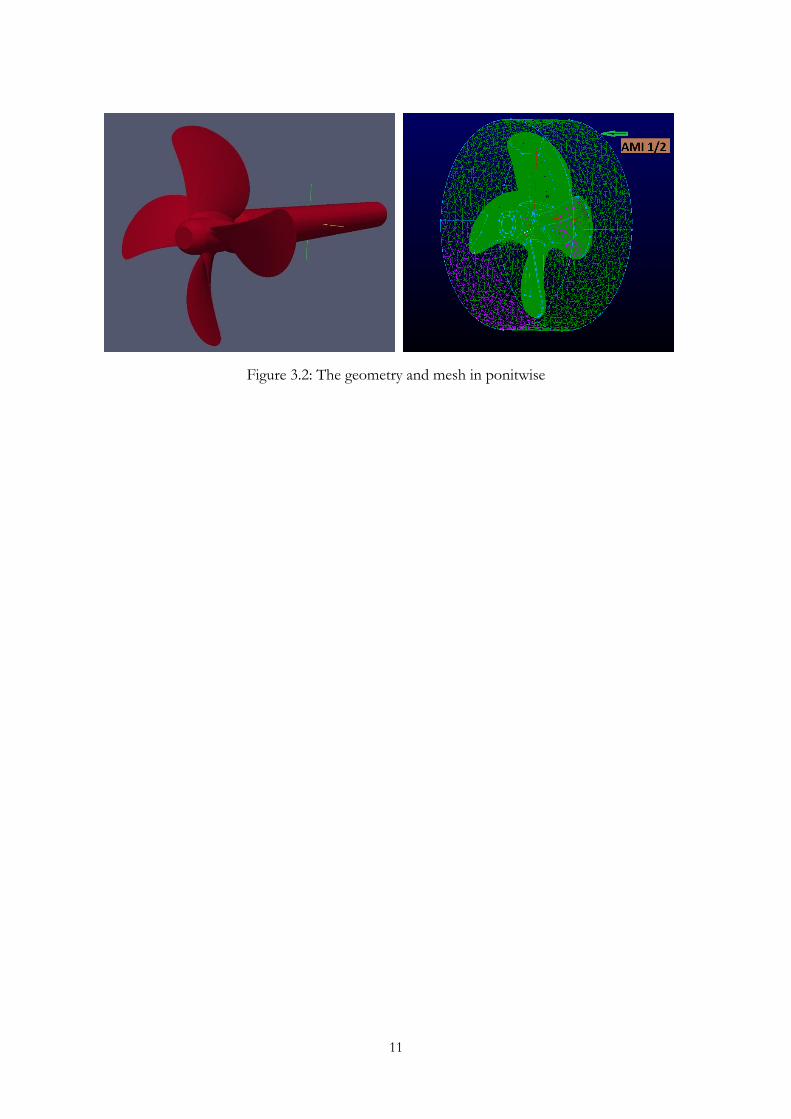
3.2 Mesh Generator Mesh generating is one of the most important steps to simulate CFD problems. Fundamentally, CFD simulations are affected by the quality of the mesh. A high-quality mesh makes CFD simulations accurately and converges quickly whereas the poor quality of the mesh can approach poor results. In order to generate mesh in this work, we used ‘’Pointwise’’ software which is a professional program to create mesh for CFD, especially for complex geometries like propeller, see Figure 3.2. Another alternative to generate mesh is to use the OpenFOAM mesher snappyHexMesh. After generating mesh in Pointwise, it will be exported to OpenFOAM that makes a folder called polyMesh that defines the geometries and characteristics of the grids. More specifically, after exporting the mesh to OpenFOAM and creating the case, to check the validity of the mesh, we can use ‘’checkMesh’’ command. It gives required information about the quality of the mesh such as number of the cells, domain size, the boundary conditions and mesh error and, etc.

11

Figure 3.2: The geometry and mesh in ponitwise

12

4 Workplan of Model Tests This chapter deals with the propeller geometry and main ship particulars which are the basis for the CFD analysis. It also explains the experimental set-up, the boundary conditions and further details about the implementations of the solvers.

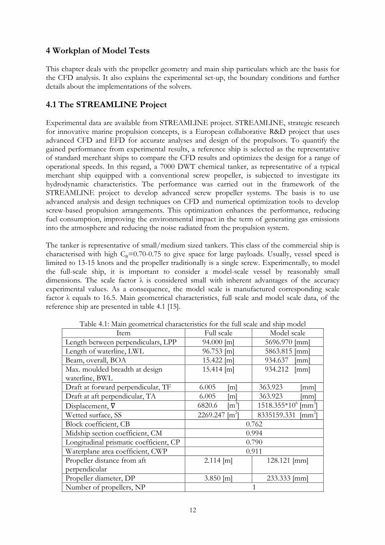
4.1 The STREAMLINE Project Experimental data are available from STREAMLINE project. STREAMLINE, strategic research for innovative marine propulsion concepts, is a European collaborative R&D project that uses advanced CFD and EFD for accurate analyses and design of the propulsors. To quantify the gained performance from experimental results, a reference ship is selected as the representative of standard merchant ships to compare the CFD results and optimizes the design for a range of operational speeds. In this regard, a 7000 DWT chemical tanker, as representative of a typical merchant ship equipped with a conventional screw propeller, is subjected to investigate its hydrodynamic characteristics. The performance was carried out in the framework of the STREAMLINE project to develop advanced screw propeller systems. The basis is to use advanced analysis and design techniques on CFD and numerical optimization tools to develop screw-based propulsion arrangements. This optimization enhances the performance, reducing fuel consumption, improving the environmental impact in the term of generating gas emissions into the atmosphere and reducing the noise radiated from the propulsion system. The tanker is representative of small/medium sized tankers. This class of the commercial ship is characterised with high CB=0.70-0.75 to give space for large payloads. Usually, vessel speed is limited to 13-15 knots and the propeller traditionally is a single screw. Experimentally, to model the full-scale ship, it is important to consider a model-scale vessel by reasonably small dimensions. The scale factor λ is considered small with inherent advantages of the accuracy experimental values. As a consequence, the model scale is manufactured corresponding scale factor λ equals to 16.5. Main geometrical characteristics, full scale and model scale data, of the reference ship are presented in table 4.1 [15].

Table 4.1: Main geometrical characteristics for the full scale and ship model

Item Full scale Model scale

Length between perpendiculars, LPP 94.000 [m] 5696.970 [mm]

Length of waterline, LWL 96.753 [m] 5863.815 [mm]

Beam, overall, BOA 15.422 [m] 934.637 [mm]

Max. moulded breadth at design waterline, BWL

15.414 [m] 934.212 [mm]

Draft at forward perpendicular, TF 6.005 [m] 363.923 [mm]

Draft at aft perpendicular, TA 6.005 [m] 363.923 [mm]

Displacement, 6820.6 [m3] 1518.355*106 [mm3]

Wetted surface, SS 2269.247 [m2] 8335159.331 [mm2]

Block coefficient, CB 0.762

Midship section coefficient, CM 0.994

Longitudinal prismatic coefficient, CP 0.790

Waterplane area coefficient, CWP 0.911

Propeller distance from aft perpendicular

2.114 [m] 128.121 [mm]

Propeller diameter, DP 3.850 [m] 233.333 [mm]

Number of propellers, NP 1

13

Full scale ship involves a four-bladed fixed-pitch propeller with diameter 3.850 m. The scale factor λ=16.5 yields a model diameter with diameter DP=233.33 mm. Geometry characteristics of the propeller is summarised in table 4.2. The dimensions are related to the model scale whereas the non-dimensional data is referred to the propeller diameter DP.

Table 4.2: Geometry characteristics of the propeller

Diameter, DP [mm] 233.33

Number of blades, N 4 (fixed pitch)

Rotation right handed

Nominal pitch ratio, (P/D0.7R) 1.0

Skew angle [deg] 13.0

Rake angle [deg] 3.0

Expanded area ratio, EAR (approx.) 0.58

Boss diameter ratio, DH/DP (at prop. disc) 0.168

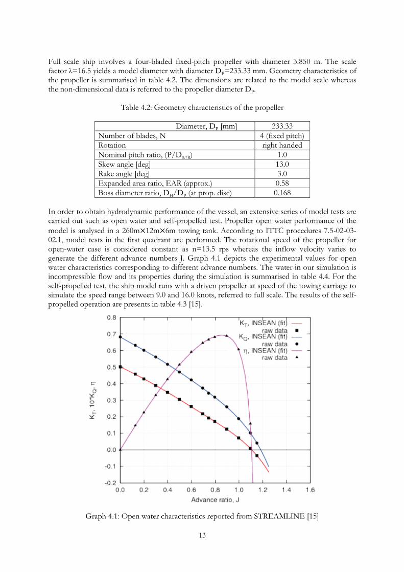
In order to obtain hydrodynamic performance of the vessel, an extensive series of model tests are carried out such as open water and self-propelled test. Propeller open water performance of the

model is analysed in a 260m 12m 6m towing tank. According to ITTC procedures 7.5-02-03-02.1, model tests in the first quadrant are performed. The rotational speed of the propeller for open-water case is considered constant as n=13.5 rps whereas the inflow velocity varies to generate the different advance numbers J. Graph 4.1 depicts the experimental values for open water characteristics corresponding to different advance numbers. The water in our simulation is incompressible flow and its properties during the simulation is summarised in table 4.4. For the self-propelled test, the ship model runs with a driven propeller at speed of the towing carriage to simulate the speed range between 9.0 and 16.0 knots, referred to full scale. The results of the self-propelled operation are presents in table 4.3 [15].

Graph 4.1: Open water characteristics reported from STREAMLINE [15]

14

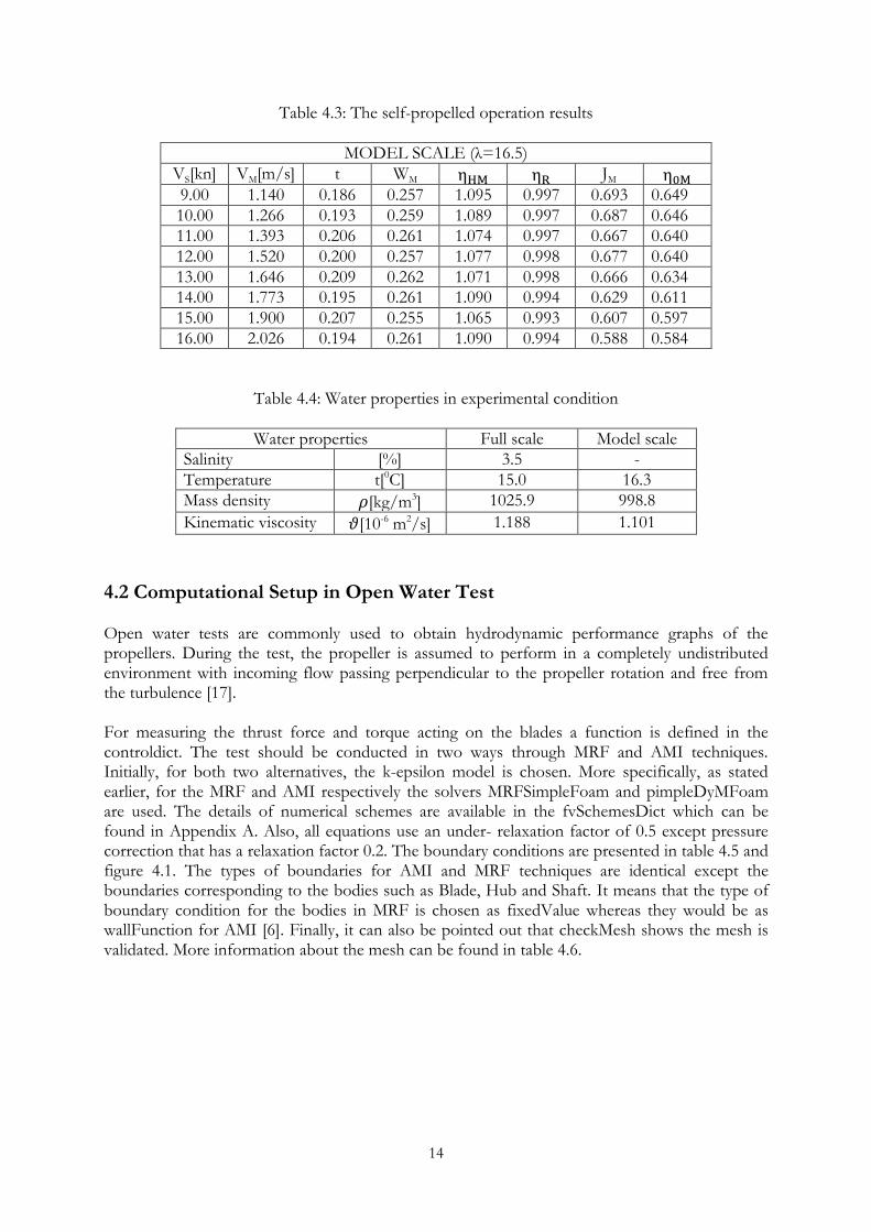
Table 4.3: The self-propelled operation results

MODEL SCALE (λ=16.5)

VS[kn] VM[m/s] t WM JM 9.00 1.140 0.186 0.257 1.095 0.997 0.693 0.649

10.00 1.266 0.193 0.259 1.089 0.997 0.687 0.646

11.00 1.393 0.206 0.261 1.074 0.997 0.667 0.640

12.00 1.520 0.200 0.257 1.077 0.998 0.677 0.640

13.00 1.646 0.209 0.262 1.071 0.998 0.666 0.634

14.00 1.773 0.195 0.261 1.090 0.994 0.629 0.611

15.00 1.900 0.207 0.255 1.065 0.993 0.607 0.597

16.00 2.026 0.194 0.261 1.090 0.994 0.588 0.584

Table 4.4: Water properties in experimental condition

Water properties Full scale Model scale

Salinity [%] 3.5 -

Temperature t[0C] 15.0 16.3

Mass density [kg/m3] 1025.9 998.8

Kinematic viscosity [10-6 m2/s] 1.188 1.101

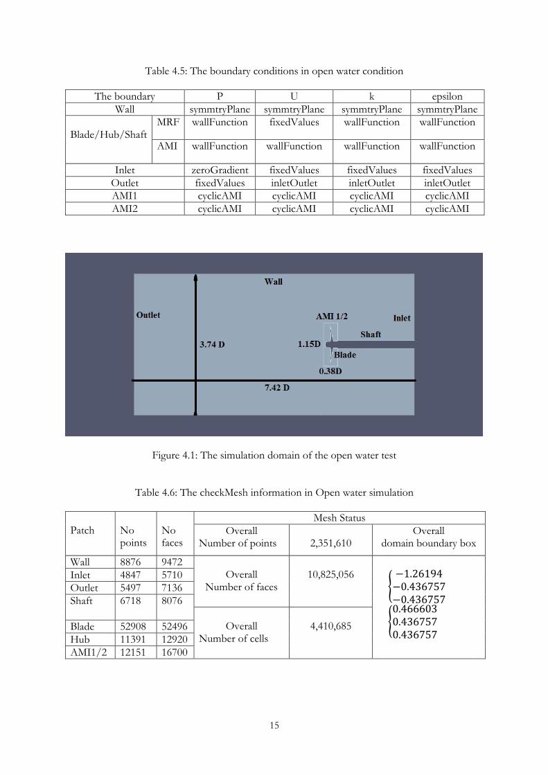
4.2 Computational Setup in Open Water Test Open water tests are commonly used to obtain hydrodynamic performance graphs of the propellers. During the test, the propeller is assumed to perform in a completely undistributed environment with incoming flow passing perpendicular to the propeller rotation and free from the turbulence [17]. For measuring the thrust force and torque acting on the blades a function is defined in the controldict. The test should be conducted in two ways through MRF and AMI techniques. Initially, for both two alternatives, the k-epsilon model is chosen. More specifically, as stated earlier, for the MRF and AMI respectively the solvers MRFSimpleFoam and pimpleDyMFoam are used. The details of numerical schemes are available in the fvSchemesDict which can be found in Appendix A. Also, all equations use an under- relaxation factor of 0.5 except pressure correction that has a relaxation factor 0.2. The boundary conditions are presented in table 4.5 and figure 4.1. The types of boundaries for AMI and MRF techniques are identical except the boundaries corresponding to the bodies such as Blade, Hub and Shaft. It means that the type of boundary condition for the bodies in MRF is chosen as fixedValue whereas they would be as wallFunction for AMI [6]. Finally, it can also be pointed out that checkMesh shows the mesh is validated. More information about the mesh can be found in table 4.6.

15

Table 4.5: The boundary conditions in open water condition

The boundary P U k epsilon

Wall symmtryPlane symmtryPlane symmtryPlane symmtryPlane

Blade/Hub/Shaft

MRF wallFunction fixedValues wallFunction wallFunction

AMI wallFunction wallFunction wallFunction wallFunction

Inlet zeroGradient fixedValues fixedValues fixedValues

Outlet fixedValues inletOutlet inletOutlet inletOutlet

AMI1 cyclicAMI cyclicAMI cyclicAMI cyclicAMI

AMI2 cyclicAMI cyclicAMI cyclicAMI cyclicAMI

Figure 4.1: The simulation domain of the open water test

Table 4.6: The checkMesh information in Open water simulation

Patch

No points

No faces

Mesh Status

Overall Number of points

2,351,610

Overall domain boundary box

Wall 8876 9472 Overall

Number of faces

10,825,056

{

{

Inlet 4847 5710

Outlet 5497 7136

Shaft 6718 8076

Overall

Number of cells

4,410,685 Blade 52908 52496

Hub 11391 12920

AMI1/2 12151 16700

16

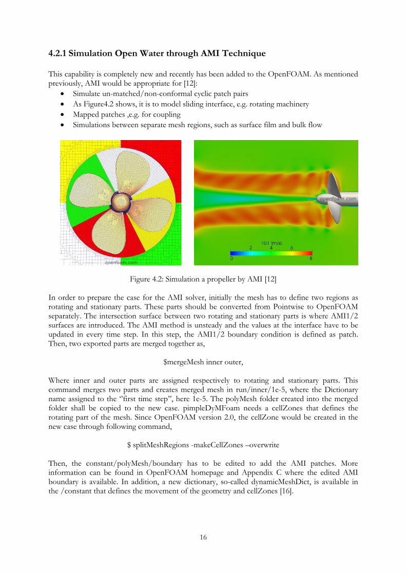
4.2.1 Simulation Open Water through AMI Technique This capability is completely new and recently has been added to the OpenFOAM. As mentioned previously, AMI would be appropriate for [12]:

Simulate un-matched/non-conformal cyclic patch pairs

As Figure4.2 shows, it is to model sliding interface, e.g. rotating machinery

Mapped patches ,e.g. for coupling

Simulations between separate mesh regions, such as surface film and bulk flow

Figure 4.2: Simulation a propeller by AMI [12] In order to prepare the case for the AMI solver, initially the mesh has to define two regions as rotating and stationary parts. These parts should be converted from Pointwise to OpenFOAM separately. The intersection surface between two rotating and stationary parts is where AMI1/2 surfaces are introduced. The AMI method is unsteady and the values at the interface have to be updated in every time step. In this step, the AMI1/2 boundary condition is defined as patch. Then, two exported parts are merged together as,

$mergeMesh inner outer,

Where inner and outer parts are assigned respectively to rotating and stationary parts. This command merges two parts and creates merged mesh in run/inner/1e-5, where the Dictionary name assigned to the ‘’first time step’’, here 1e-5. The polyMesh folder created into the merged folder shall be copied to the new case. pimpleDyMFoam needs a cellZones that defines the rotating part of the mesh. Since OpenFOAM version 2.0, the cellZone would be created in the new case through following command,

$ splitMeshRegions -makeCellZones –overwrite

Then, the constant/polyMesh/boundary has to be edited to add the AMI patches. More information can be found in OpenFOAM homepage and Appendix C where the edited AMI boundary is available. In addition, a new dictionary, so-called dynamicMeshDict, is available in the /constant that defines the movement of the geometry and cellZones [16].

17

4.2.2 Simulation Open Water through MRF Technique In order to model the propeller in this steady state method, we divide the calculation zones in two different cylindrical domains, moving and stationary zones. The size of this domain is dependent on the diameter of the propeller. The aim of this zone is to simulate the movement of the propeller and hub by applying the Corioilis acceleration term in the Navier Stokes equations. In this method unlike the sliding grid method, the mesh is static. It means that MRF doesn’t need to be updated in every iteration step. There are several ways to prepare the case for MRF. First, it should be used the stitchMesh utility of OpenFOAM. In this regard similar what we did for AMI, the merged mesh must be stitched as

$stitchMesh –perfect inner outer

It should be noted that if the number of cells assigned to AMI boundaries and boundary mesh on each interface are identical and matched up,’’-perfect ‘’ should be used otherwise it is ‘’-partial’’. In the MRF method, MRFZones, located in the constant, introduces which part relates to the reference frame, also the origin axis and the rotation of the rotor. Normally, employing the stitchMesh utility is difficult to control and can lead some problems in mesh quality, especially when the geometry becomes complex for instance in self-propulsion test. An alternative might be similar with the AMI set-up, without stitching and by removing the AMI boundaries but the AMI1/2 must be added in the MRFZones as non-rotational zones. In this thesis it has been used due to its implementation is easier especially when we perform the self-propelled case.

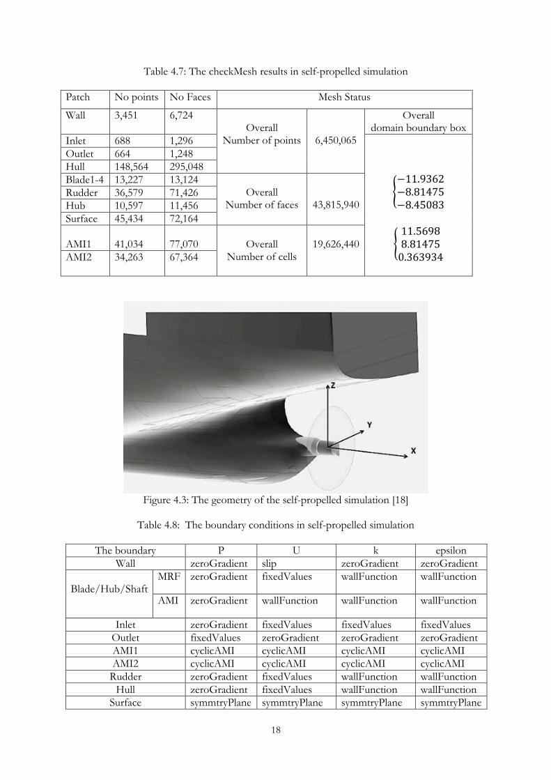
4.3 Computational Setup in Self-propelled Test Alike the open water condition, self-propelled test will be conducted in two ways, using AMI and MRF techniques. The tests were performed on a reference ship in the speed range of 9.0 and 16.0 knots in the large towing tank, observe table 4.3. The CFD simulation is performed only for j=0.629 corresponding to the speed of the full-scale ship V=14 knots or Vs=1.773 m/s in model-scale case. The geometry is more complex than the open-water case and requires longer time and large number of nodes to run by computer Cluster. We use the cyclicAMI boundary conditions instead of the stitching alternative. Also, we considered identical numerical schemes and characteristics, turbulence model and the solvers with open-water test. The mesh is also verified after using ‘’checkMesh’’ and the results are presented in table 4.7. The boundary conditions, and the geometry are presented in table 4.8 and figure 4.3.

18

Table 4.7: The checkMesh results in self-propelled simulation

Patch No points No Faces Mesh Status

Wall 3,451 6,724 Overall

Number of points

6,450,065

Overall domain boundary box

Inlet 688 1,296

Outlet 664 1,248

Hull 148,564 295,048

Blade1-4 13,227 13,124 Overall

Number of faces

43,815,940

{

Rudder 36,579 71,426

Hub 10,597 11,456

Surface 45,434 72,164

AMI1

41,034

77,070

Overall

Number of cells

19,626,440 {

AMI2

34,263 67,364

Figure 4.3: The geometry of the self-propelled simulation [18]

Table 4.8: The boundary conditions in self-propelled simulation

The boundary P U k epsilon

Wall zeroGradient slip zeroGradient zeroGradient

Blade/Hub/Shaft

MRF zeroGradient fixedValues wallFunction wallFunction

AMI zeroGradient wallFunction wallFunction wallFunction

Inlet zeroGradient fixedValues fixedValues fixedValues

Outlet fixedValues zeroGradient zeroGradient zeroGradient

AMI1 cyclicAMI cyclicAMI cyclicAMI cyclicAMI

AMI2 cyclicAMI cyclicAMI cyclicAMI cyclicAMI

Rudder zeroGradient fixedValues wallFunction wallFunction

Hull zeroGradient fixedValues wallFunction wallFunction

Surface symmtryPlane symmtryPlane symmtryPlane symmtryPlane

19

5 Results and Discussions In this chapter the results from the simulations are presented to validate their accuracy. First, the open-water computational results in different advance numbers for the MRF and AMI models are investigated. Then, scalability analyses on the open-water case are studied to get a deeper understanding of how the computation should be configured to approach optimum number of processors within parallel set-up. Finally, in the self-propulsion condition, the flow field will be studied in order to compute the thrust force and torque acting on the blades. In this section, as a starting point, we employ standard k-epsilon as the main turbulence model and then we proceed the implementation with different turbulence models to find out dependency of turbulence models on the numerical predictions.

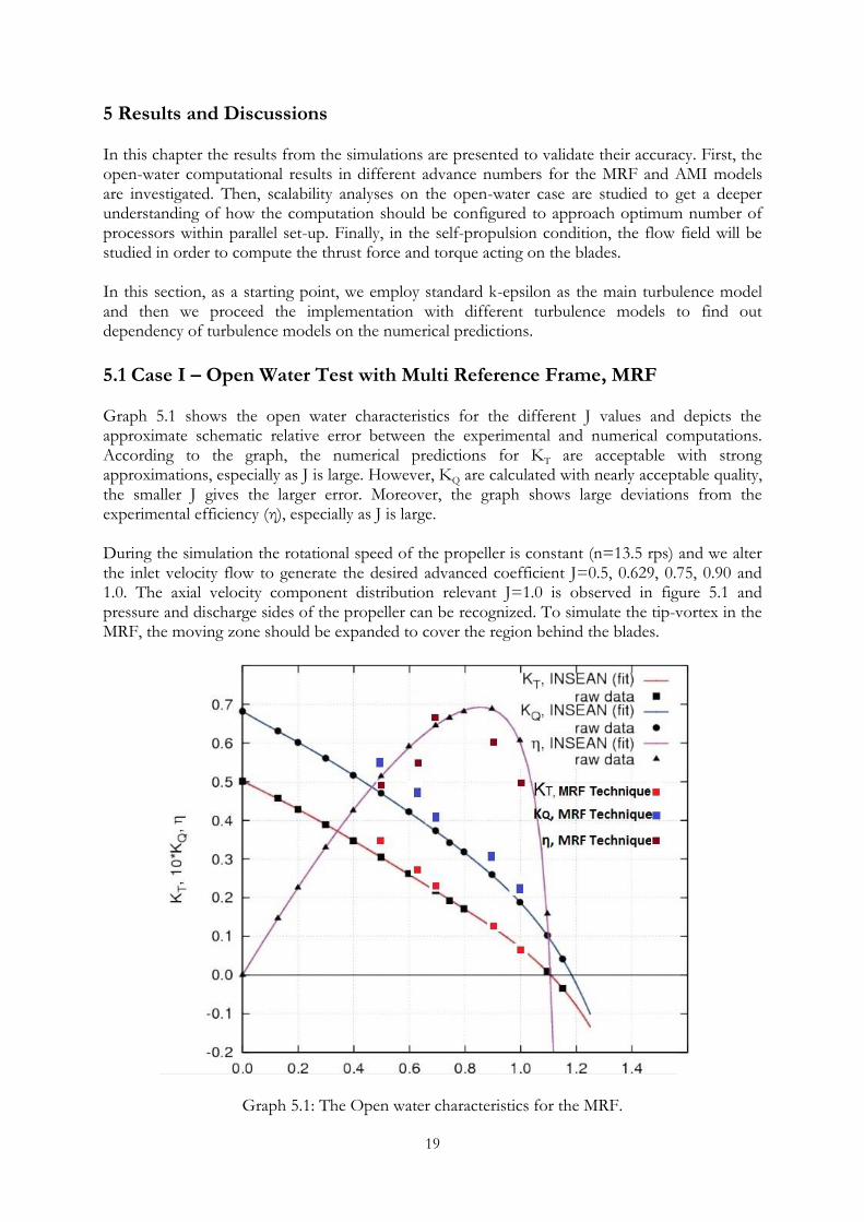
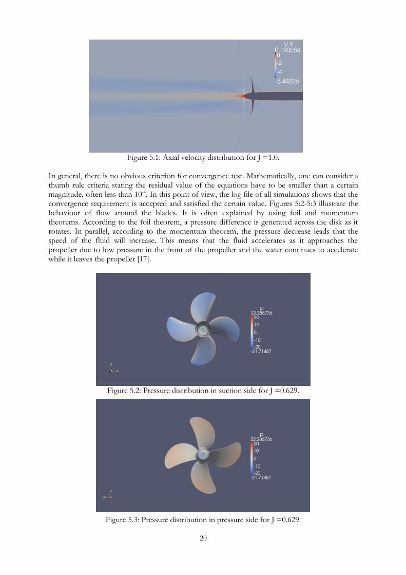
5.1 Case I – Open Water Test with Multi Reference Frame, MRF Graph 5.1 shows the open water characteristics for the different J values and depicts the approximate schematic relative error between the experimental and numerical computations. According to the graph, the numerical predictions for KT are acceptable with strong approximations, especially as J is large. However, KQ are calculated with nearly acceptable quality, the smaller J gives the larger error. Moreover, the graph shows large deviations from the experimental efficiency (η), especially as J is large. During the simulation the rotational speed of the propeller is constant (n=13.5 rps) and we alter the inlet velocity flow to generate the desired advanced coefficient J=0.5, 0.629, 0.75, 0.90 and 1.0. The axial velocity component distribution relevant J=1.0 is observed in figure 5.1 and pressure and discharge sides of the propeller can be recognized. To simulate the tip-vortex in the MRF, the moving zone should be expanded to cover the region behind the blades.

Graph 5.1: The Open water characteristics for the MRF.

20

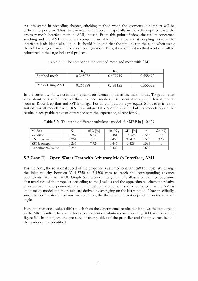
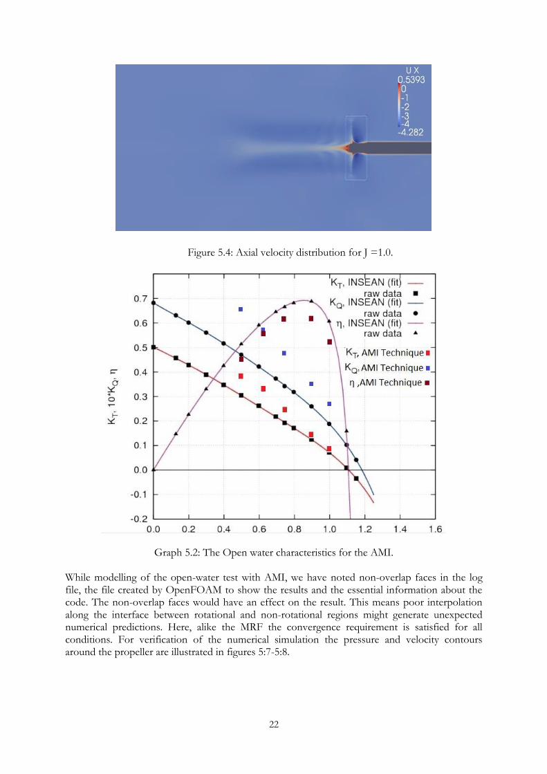
Figure 5.1: Axial velocity distribution for J =1.0. In general, there is no obvious criterion for convergence test. Mathematically, one can consider a thumb rule criteria stating the residual value of the equations have to be smaller than a certain magnitude, often less than 10-4. In this point of view, the log file of all simulations shows that the convergence requirement is accepted and satisfied the certain value. Figures 5:2-5:3 illustrate the behaviour of flow around the blades. It is often explained by using foil and momentum theorems. According to the foil theorem, a pressure difference is generated across the disk as it rotates. In parallel, according to the momentum theorem, the pressure decrease leads that the speed of the fluid will increase. This means that the fluid accelerates as it approaches the propeller due to low pressure in the front of the propeller and the water continues to accelerate while it leaves the propeller [17].

Figure 5.2: Pressure distribution in suction side for J =0.629.

Figure 5.3: Pressure distribution in pressure side for J =0.629.

21

As it is stated in preceding chapter, stitching method when the geometry is complex will be difficult to perform. Thus, to eliminate this problem, especially in the self-propelled case, the arbitrary mesh interface method, AMI, is used. From this point of view, the results concerned stitching and the AMI method are compared in table 5.1. It proves that coupling between the interfaces leads identical solution. It should be noted that the time to run the code when using the AMI is longer than stitched mesh configuration. Thus, if the stitched method works, it will be prioritized in the large industrial projects.

Table 5.1: The comparing the stitched mesh and mesh with AMI

Item KT KQ η

Stitched mesh 0.265072 0.477719

0.555472

Mesh Using AMI 0.266888 0.481122 0.555322

In the current work, we used the k-epsilon turbulence model as the main model. To get a better view about on the influence of the turbulence models, it is essential to apply different models such as RNG k-epsilon and SST k-omega. For all computations y+ equals 5 however it is not suitable for all models except RNG k-epsilon. Table 5.2 shows all turbulence models obtain the results in acceptable range of difference with the experience, except for KQ.

Table 5.2: The testing different turbulence models for MRF in J=0.629

Models KT ΔKT [%] 10×KQ ΔKQ [%] η Δη [%]

k-epsilon 0.267 8.537 0.481 14.524 0.555 7.5

RNG k-epsilon 0.264 7.317 0.458 9.0476 0.578 3.67

SST k-omega 0.265 7.724 0.447 6.429 0.594 1

Experimental value 0.246 - 0.420 - 0.600 -

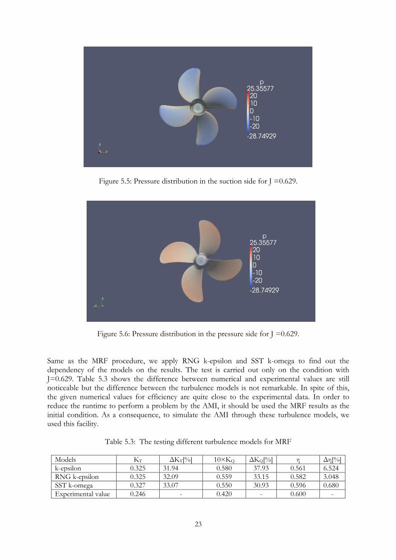
5.2 Case II – Open Water Test with Arbitrary Mesh Interface, AMI For the AMI, the rotational speed of the propeller is assumed constant (n=13.5 rps) .We change the inlet velocity between V=1.5750 to 3.1500 m/s to reach the corresponding advance coefficients J=0.5 to J=1.0. Graph 5.2, identical to graph 5.1, illustrates the hydrodynamic characteristics of the propeller according to the J values and the approximate schematic relative error between the experimental and numerical computations. It should be noted that the AMI is an unsteady model and the results are derived by averaging on the last rotation. More specifically, since the open water is a symmetric condition, the thrust force is not dependent on the rotation angle. Here, the numerical values differ much from the experimental results but it shows the same trend as the MRF results. The axial velocity component distribution corresponding J=1.0 is observed in figure 5.6. In this figure the pressure, discharge sides of the propeller and the tip vortex behind the blades can be identified.

22

Figure 5.4: Axial velocity distribution for J =1.0.

Graph 5.2: The Open water characteristics for the AMI.

While modelling of the open-water test with AMI, we have noted non-overlap faces in the log file, the file created by OpenFOAM to show the results and the essential information about the code. The non-overlap faces would have an effect on the result. This means poor interpolation along the interface between rotational and non-rotational regions might generate unexpected numerical predictions. Here, alike the MRF the convergence requirement is satisfied for all conditions. For verification of the numerical simulation the pressure and velocity contours around the propeller are illustrated in figures 5:7-5:8.

23

Figure 5.5: Pressure distribution in the suction side for J =0.629.

Figure 5.6: Pressure distribution in the pressure side for J =0.629.

Same as the MRF procedure, we apply RNG k-epsilon and SST k-omega to find out the dependency of the models on the results. The test is carried out only on the condition with J=0.629. Table 5.3 shows the difference between numerical and experimental values are still noticeable but the difference between the turbulence models is not remarkable. In spite of this, the given numerical values for efficiency are quite close to the experimental data. In order to reduce the runtime to perform a problem by the AMI, it should be used the MRF results as the initial condition. As a consequence, to simulate the AMI through these turbulence models, we used this facility.

Table 5.3: The testing different turbulence models for MRF

Models KT ΔKT[%] 10×KQ ΔKQ[%] η Δη[%]

k-epsilon 0.325 31.94 0.580 37.93 0.561 6.524

RNG k-epsilon 0.325 32.09 0.559 33.15 0.582 3.048

SST k-omega 0.327 33.07 0.550 30.93 0.596 0.680

Experimental value 0.246 - 0.420 - 0.600 -

24

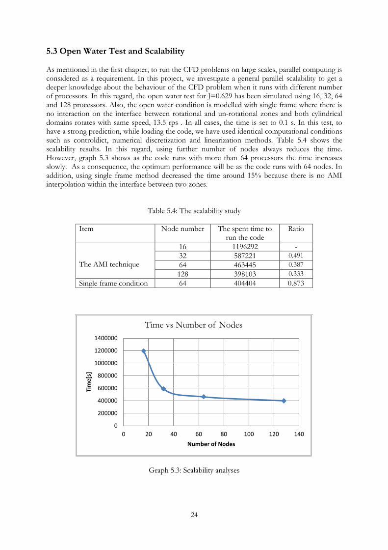
5.3 Open Water Test and Scalability As mentioned in the first chapter, to run the CFD problems on large scales, parallel computing is considered as a requirement. In this project, we investigate a general parallel scalability to get a deeper knowledge about the behaviour of the CFD problem when it runs with different number of processors. In this regard, the open water test for J=0.629 has been simulated using 16, 32, 64 and 128 processors. Also, the open water condition is modelled with single frame where there is no interaction on the interface between rotational and un-rotational zones and both cylindrical domains rotates with same speed, 13.5 rps . In all cases, the time is set to 0.1 s. In this test, to have a strong prediction, while loading the code, we have used identical computational conditions such as controldict, numerical discretization and linearization methods. Table 5.4 shows the scalability results. In this regard, using further number of nodes always reduces the time. However, graph 5.3 shows as the code runs with more than 64 processors the time increases slowly. As a consequence, the optimum performance will be as the code runs with 64 nodes. In addition, using single frame method decreased the time around 15% because there is no AMI interpolation within the interface between two zones.

Table 5.4: The scalability study

Item Node number The spent time to run the code

Ratio

The AMI technique

16 1196292 -

32 587221 0.491

64 463445 0.387

128 398103 0.333

Single frame condition 64 404404 0.873

Graph 5.3: Scalability analyses

0

200000

400000

600000

800000

1000000

1200000

1400000

0 20 40 60 80 100 120 140

Tim

e[s

]

Number of Nodes

Time vs Number of Nodes

25

5.4 Self-propulsion Test After determining the resistance of the scale model ship along a resistance test in a towing tank, the next step is self-propulsion test where the model is propelled by its own propeller. The test is performed to evaluate the required power and the rotational speed of the propeller when the full-scale ship is moving in the service speed. The experimental tests were carried out in the speed range of 9.0 and 16.0 knots. In this thesis, we investigate validation of the numerical methods when the model-scale ship performs in J=0.629 and inflow velocity is 1.77 m/s (Froude = 0.23), corresponding to the full-scale ship service speed V=14 knots. Here, In contrast with the open-water case, the interaction between hull and propeller is not axisymmetric, see figure4.4. As a consequence, the flow field around the propeller is dependent on the positions of the blades and the hull. In this test, the grid around the propeller is identical to the open water case and the turbulence model is RNG k-epsilon to simulate the test for the MRF and AMI techniques and y+ is around 5.

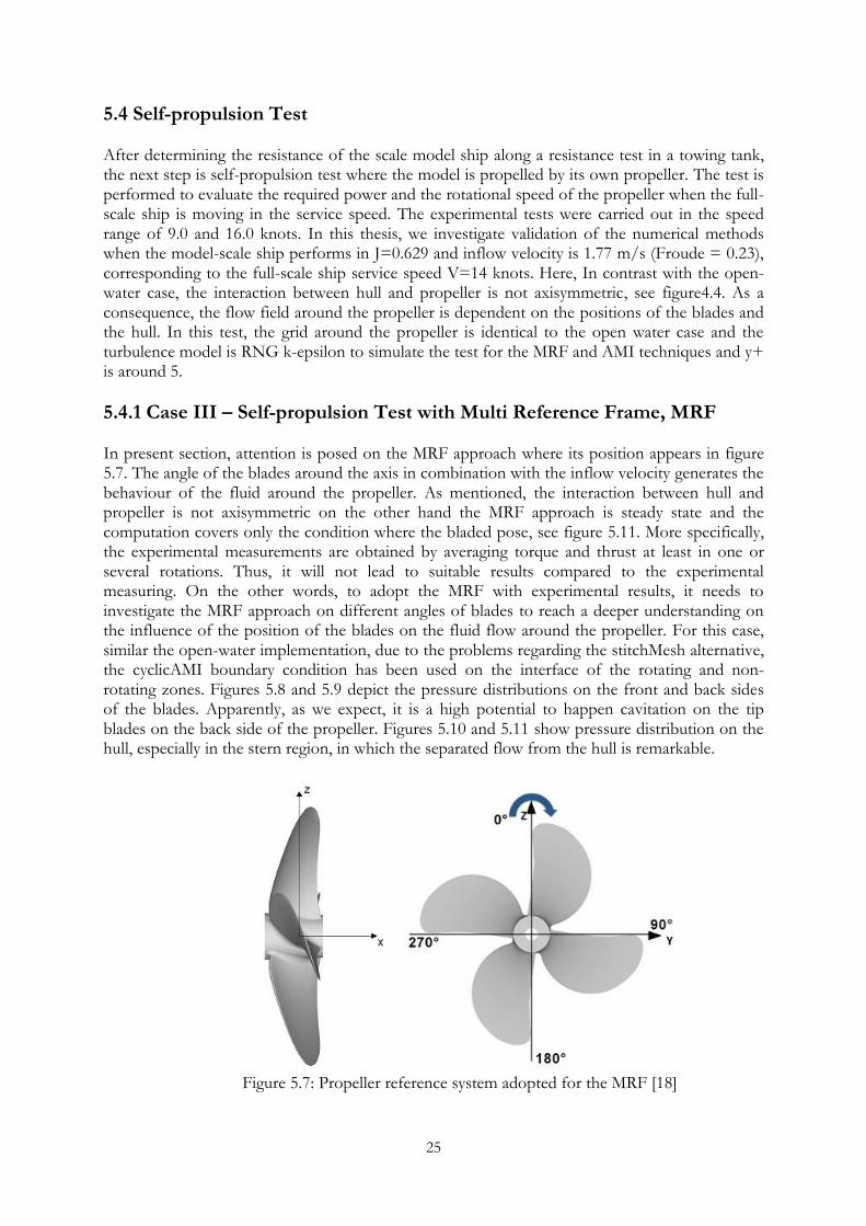
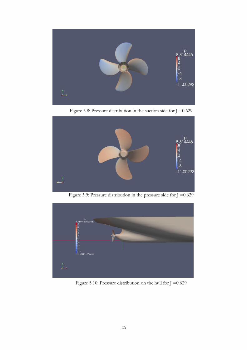
5.4.1 Case III – Self-propulsion Test with Multi Reference Frame, MRF In present section, attention is posed on the MRF approach where its position appears in figure 5.7. The angle of the blades around the axis in combination with the inflow velocity generates the behaviour of the fluid around the propeller. As mentioned, the interaction between hull and propeller is not axisymmetric on the other hand the MRF approach is steady state and the computation covers only the condition where the bladed pose, see figure 5.11. More specifically, the experimental measurements are obtained by averaging torque and thrust at least in one or several rotations. Thus, it will not lead to suitable results compared to the experimental measuring. On the other words, to adopt the MRF with experimental results, it needs to investigate the MRF approach on different angles of blades to reach a deeper understanding on the influence of the position of the blades on the fluid flow around the propeller. For this case, similar the open-water implementation, due to the problems regarding the stitchMesh alternative, the cyclicAMI boundary condition has been used on the interface of the rotating and non-rotating zones. Figures 5.8 and 5.9 depict the pressure distributions on the front and back sides of the blades. Apparently, as we expect, it is a high potential to happen cavitation on the tip blades on the back side of the propeller. Figures 5.10 and 5.11 show pressure distribution on the hull, especially in the stern region, in which the separated flow from the hull is remarkable.

Figure 5.7: Propeller reference system adopted for the MRF [18]

26

Figure 5.8: Pressure distribution in the suction side for J =0.629

Figure 5.9: Pressure distribution in the pressure side for J =0.629

Figure 5.10: Pressure distribution on the hull for J =0.629

27

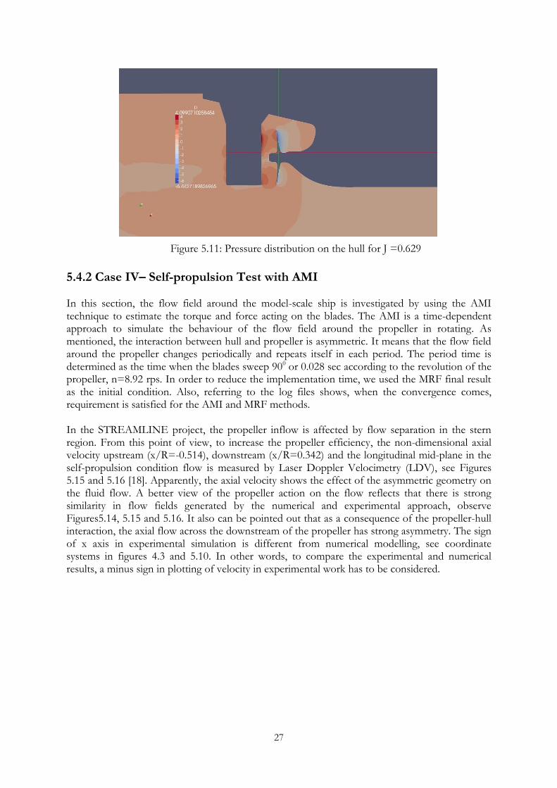
Figure 5.11: Pressure distribution on the hull for J =0.629

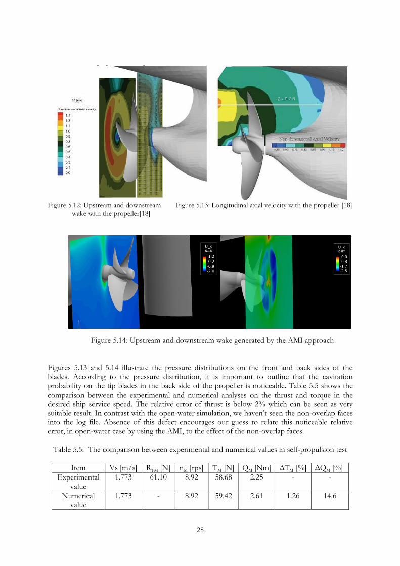
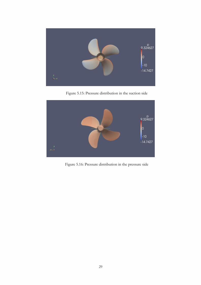
5.4.2 Case IV– Self-propulsion Test with AMI In this section, the flow field around the model-scale ship is investigated by using the AMI technique to estimate the torque and force acting on the blades. The AMI is a time-dependent approach to simulate the behaviour of the flow field around the propeller in rotating. As mentioned, the interaction between hull and propeller is asymmetric. It means that the flow field around the propeller changes periodically and repeats itself in each period. The period time is determined as the time when the blades sweep 900 or 0.028 sec according to the revolution of the propeller, n=8.92 rps. In order to reduce the implementation time, we used the MRF final result as the initial condition. Also, referring to the log files shows, when the convergence comes, requirement is satisfied for the AMI and MRF methods. In the STREAMLINE project, the propeller inflow is affected by flow separation in the stern region. From this point of view, to increase the propeller efficiency, the non-dimensional axial velocity upstream (x/R=-0.514), downstream (x/R=0.342) and the longitudinal mid-plane in the self-propulsion condition flow is measured by Laser Doppler Velocimetry (LDV), see Figures 5.15 and 5.16 [18]. Apparently, the axial velocity shows the effect of the asymmetric geometry on the fluid flow. A better view of the propeller action on the flow reflects that there is strong similarity in flow fields generated by the numerical and experimental approach, observe Figures5.14, 5.15 and 5.16. It also can be pointed out that as a consequence of the propeller-hull interaction, the axial flow across the downstream of the propeller has strong asymmetry. The sign of x axis in experimental simulation is different from numerical modelling, see coordinate systems in figures 4.3 and 5.10. In other words, to compare the experimental and numerical results, a minus sign in plotting of velocity in experimental work has to be considered.

28

Figure 5.12: Upstream and downstream Figure 5.13: Longitudinal axial velocity with the propeller [18]

wake with the propeller[18]

Figure 5.14: Upstream and downstream wake generated by the AMI approach

Figures 5.13 and 5.14 illustrate the pressure distributions on the front and back sides of the blades. According to the pressure distribution, it is important to outline that the cavitation probability on the tip blades in the back side of the propeller is noticeable. Table 5.5 shows the comparison between the experimental and numerical analyses on the thrust and torque in the desired ship service speed. The relative error of thrust is below 2% which can be seen as very suitable result. In contrast with the open-water simulation, we haven’t seen the non-overlap faces into the log file. Absence of this defect encourages our guess to relate this noticeable relative error, in open-water case by using the AMI, to the effect of the non-overlap faces.

Table 5.5: The comparison between experimental and numerical values in self-propulsion test

Item Vs [m/s] RTM [N] nM [rps] TM [N] QM [Nm] ΔTM [%] ΔQM [%]

Experimental value

1.773 61.10 8.92 58.68 2.25 - -

Numerical value

1.773 - 8.92 59.42 2.61 1.26 14.6

29

Figure 5.15: Pressure distribution in the suction side

Figure 5.16: Pressure distribution in the pressure side

30

6 Conclusions and Future Work 6.1 Conclusion The main purpose of this thesis was to approach the propeller hydrodynamic performance via numerical modelling. We have investigated the feasibility study on the use of two dynamic mesh techniques, MRF and AMI, to predict the flow around the propeller in the open-water and self-propulsion conditions. As the starting point, a study on simulating the propeller in the open-water test has been carried out to predict the hydrodynamic performance of the propeller in some advance numbers J. Then, we investigated a general parallel scalability in open-water condition for J=0.629. It got a deeper knowledge about the behaviour of the problem when it runs with different number of processors. Finally, the self-propulsion case has been studied to derive the thrust and torque which is required to run the model-scale ship in the service speed. The results of the open-water case by using the MRF method shows that the turbulence models k-Epsilon, SST k-omega and RNG-k-Epsilon are agreeing well with the experiments. However, the result corresponding SST k-omega and RNG-k-Epsilon show closer to the experimental results. Furthermore, we have investigated the stitching and using AMI alternatives to make rotating and non-rotating zones. Comparison between the methods shows identical solution that causes employing the AMI method can be prioritized. Another study was on the AMI method to model the flow field around the propeller in open-water condition. It differs much from the experiments. Despite of this, it can predict the flow field around the propeller that would be explained with the momentum and foil theorems. As running the code, it has been observed the non-overlapped faces that might effect on the accuracy. Notable is how this might affect on the result where generating a new mesh is quite difficult and time consuming. Also, applying different turbulence models show that the numerical approach is not dependent on the turbulent models. From the scalability study on the AMI, it can be seen that applying further processors always reduces the required time. It can also be pointed out that as the code runs with higher number of processors the time increases slowly. The use of higher processors is expensive, beside of the reaching shorter time by applying higher nodes, it results the optimum performance happens when the code runs with 64 processors. In addition, using single frame method decreased the time around 15% due to no interpolation within the interface between the zones. Regarding the self-propulsion test, it could be seen, the interaction between hull and propeller is asymmetric. The MRF approach is a steady state method and approaches to the averaged results in that particular blade position. Thus, in order to adopt the MRF with experimental results, it requires new attempts to simulate the flow on different positions of the blades. On the other hand, the AMI is a time-dependent approach and enables to simulate the behaviour of the flow field around the propeller in rotating. It is useful for the modelling of the interaction between hull and propeller. The relative error of thrust is below 2% which can be seen as suitable results. In contrast with the open-water condition, we haven’t realized the non-overlap faces here. Absence of this defect increases the possibility to relate the notable relative error to the effect of the non-overlap faces.

31

6.2 Future Work In recent years, the development of OpenFOAM has aided to predict ship propeller performances with acceptable accuracy. Despite the development, many different problems related to accuracy of the dynamic mesh methods still exist and needs further studies. Further developing of this thesis could be to study unfavourable wake and separated flow from the hull and investigate its effect on the propeller performance. It might cause a dramatic development on the design of the hull with low cost. Also, special attention has to be paid to study the effect of the radiated noise problems to increase environmental standard. From this point of view, new challenges are to reduce the pressure pulses and radiated noise. Thus, in self-propelled condition, the transient forces on the propeller and pressure pulses shall be evaluated. Unfortunately, we couldn’t perform a pressure pulses study on the hull due to it was not determined the pressure point reference in the STREAMLINE’s report to adopt the numerical results to the experiments. Regarding the scalability study, it would be developed further by investigating the effect of altering the number of grids and nodes. From this point of view, it should be studied the runtime when the numbers of the nodes and processors are altered with a same growth ratio, e.g. if the number of grids grows two times the number of processors will increase with a growth rate of two as well. Finally, this current study would be developed with the study on the effect of the turbulence models on the all advance numbers (J). In addition, we can assign the recommended y+ values for each turbulence models in the mesh generating. Finally, the other turbulent model such as Linear and Non-linear eddy viscosity models shall be studied to find out their effect on the numerical results.

i

Bibliography [1] Farrell P. E. and Maddison J. R., Comput. Methods Appl. Mech Engrg 200:89 (2011).

[2] L. Haakansson M. Mortensen R. Sudiyo B. Andersson, R. Andersson and B.Wachem. Computational Fluid Dynamics for Chemical Engineers. Gothenburg, Sweden, 6th edition, 2010. [3] Pope S.B., Turbulent Flows. Cambridge University Press, 2000. [4] Petit O., Towards Full Predictions of the Unsteady Incompressible Flow in Rotating Machines, Using OpenFOAM, Gothenburg, Sweden, 2012. [5] Salim .M. Salim, and Cheah S.C., Wall y+ Strategy for Dealing with Wall-bounded, Proceedings of the International MultiConference of Engineers and Computer Scientists 2009 Vol II IMECS 2009, March 18 - 20, 2009, Hong Kong. [6] MÜHLHÖLZER. ROSA, Feasibility Study on the Use of Multiple-Reference Frames for Computations of Propeller-Hull Interaction in OpenFOAM®, Gothenburg, Sweden, 2012. [7] Klerebrant Klasson. Olof, A Validation, Comparison and Automation of Different Computational Tools for Propeller Open Water Predictions, Gothenburg, Sweden, 2011. [8] Shang Zhi., Performance analysis of large scale parallel CFD computing based on Code_Saturne , Department of Computational Science and Engineering, Science and Technology Facilities Council, Daresbury Laboratory, Warrington WA4 4AD, United Kingdom. [9] CHEN .Jian-zhen, LI .Bin, SHEN .Dan-ping., The Multi-core CPU Parallel Computation for CFD Simulation of Flowmeter, 2008 International Symposium on Information Science and Engieering. [10] ANSYS, Inc. ANSYS FLUENT 12.0 - Theory guide, 2009. [11] STREAMLINE, D35.1 – Mesh Coupling Using A Sliding Grid Approach, October 2011. [12] The OpenFOAM Foundation. www.openfoam.org,2013. Ltd. OpenCFD. OpenFOAM - User guide- Version 2.1.0, 2011. [13] Garme K., Ship Resistance and Powering, KTH Marina Center, Stockholm 2011.

[14] www.wikipedia.org, 2013. [15] STREAMLINE, Deliverable D21.1- Results of model tests on reference configurations, August 2011. [16] AKIMOTO.H, Division of Ocean Systems Engineering (OSE), Korea Advanced Institute of Science and Technology, Dynamic mesh control. [17] Kuttenkeuler J., propeller Analysis, KTH Marina Center, Stockholm 2010.

ii

[18] Pecoraro Andrea, Di Felice Fabio, Felli Mario, Salvatore Francesco, Viviani Michele, Propeller-hull interaction in a single-screw vessel, Third International Symposium on Marine Propulsorssmp’13, Launceston, Tasmania, Australia, May 2013. [19] Nakisa. Mehdi, Abbasi. Mohammad Javad, MobasherAmini. Ahmad. Assessment of Marine Propeller Hydrodynamic Performance In Open Water Via CFD, The International Conference on Marine Technology, December 2010, BUET, Dhaka, Bangladesh.

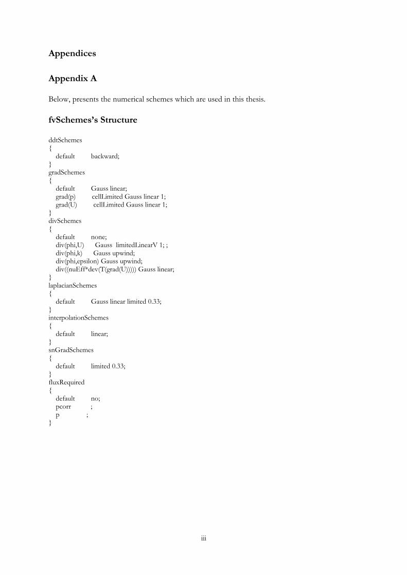
iii

Appendices

Appendix A Below, presents the numerical schemes which are used in this thesis.

fvSchemes’s Structure ddtSchemes { default backward; } gradSchemes { default Gauss linear; grad(p) cellLimited Gauss linear 1; grad(U) cellLimited Gauss linear 1; } divSchemes { default none; div(phi,U) Gauss limitedLinearV 1; ; div(phi,k) Gauss upwind; div(phi,epsilon) Gauss upwind; div((nuEff*dev(T(grad(U))))) Gauss linear; } laplacianSchemes { default Gauss linear limited 0.33; } interpolationSchemes { default linear; } snGradSchemes { default limited 0.33; } fluxRequired { default no; pcorr ; p ; }

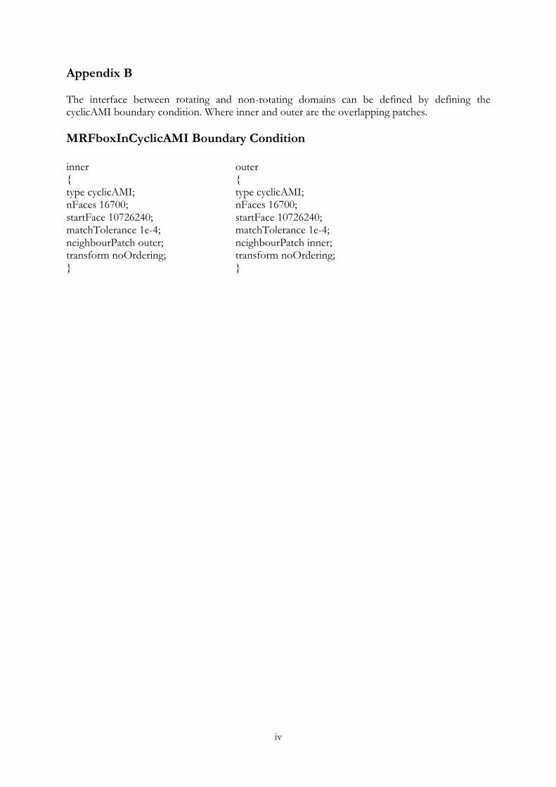
iv

Appendix B The interface between rotating and non-rotating domains can be defined by defining the cyclicAMI boundary condition. Where inner and outer are the overlapping patches.

MRFboxInCyclicAMI Boundary Condition inner { type cyclicAMI; nFaces 16700; startFace 10726240; matchTolerance 1e-4; neighbourPatch outer; transform noOrdering; }

outer { type cyclicAMI; nFaces 16700; startFace 10726240; matchTolerance 1e-4; neighbourPatch inner; transform noOrdering; }