Embed Size (px)
Citation preview

Properties of Halo Nuclei
from Atomic Isotope Shifts
Gordon W.F. Drake
University of Windsor, Canada
Collaborators
Zong-Chao Yan (UNB)
Mark Cassar (A.I.P.)
Zheng Zhong (Ph.D. student)
Qixue Wu (Ph.D. student)
Atef Titi (Ph.D. student)
Razvan Nistor (M.Sc. completed)
Levent Inci (M.Sc. completed)
Financial Support: NSERC and SHARCnet
Few Body 18 ConferenceSao Paulo, Brazil22 August 2006
semin00.tex, August 2006

Halo Nuclei Halo Nuclei 66He and He and 88HeHe
Borromean
Isotope Half-life Spin Isospin Core + Valence
He-6 807 ms 0+ 1 α + 2n
He-8 119 ms 0+ 2 α + 4n
I. Tanihata et al., Phys. Lett. (1992)
( ) ( ) ( )26 4 6I I nHe He Heσ σ σ−− =
( ) ( ) ( ) ( )2 48 4 8 8I I n nHe He He Heσ σ σ σ− −− = +
( ) ( ) ( )28 6 8I I nHe He Heσ σ σ−− ≠
Core-Halo Structure3.0
2.5
2.0
1.5
1.0
Inte
ract
ion
Rad
ius
(fm)
876543
Helium Mass Number A
I. Tanihata et al., Phys. Lett. (1985)

Charge Radii MeasurementsCharge Radii Measurements
Methods of measuring nuclear radii (interaction radii, matter radii, charge radii)Nuclear scattering – model dependentElectron scattering – stable isotope onlyMuonic atom spectroscopy – stable isotope onlyAtomic isotope shift
He-3 He-4 He-6 He-8QMC Theory 1.74(1) 1.45(1) 1.89(1) 1.86(1)
µ-He Lamb Shift 1.474(7)
Atomic Isotope Shift 1.766(6) ? ?p-He Scattering 1.95(10) GG
1.81(09) GO1.68(7) GG1.42(7) GO
RMS point proton radii (fm) from theory and experiment
G.D. Alkhazov et al., Phys. Rev. Lett. 78, 2313 (1997);D. Shiner et al., Phys. Rev. Lett. 74, 3553 (1995).
6He

Laser Spectroscopic Determination of the Nuclear Charge Radius oLaser Spectroscopic Determination of the Nuclear Charge Radius off 66HeHe
6He: 4He + 2nIts charge radius expands due to the motion of the 4He core
Motivation • Test the Standard Nuclear Structure Model;• Study nucleon interactions in neutron-rich matter.
Method: Atomic isotope shift6He – 4He isotope shift at 2 3S1 – 3 3P2 , 389 nmIS (MHz) = 43,196.202(20) + 1.008 x [<r2>4He - <r2>6He]
-- G.W.F. Drake, Nucl. Phys. A737c, 25 (2004)
L.-B. Wang, P. Mueller, K. Bailey, J.P. Greene, D. Henderson, R.J. Holt, R.V.F. Janssens, C.L. Jiang, Z.-T. Lu, T.P. O'Connor, R.C. Pardo, K.E. Rehm, J.P. Schiffer, X.D. Tang Argonne National Lab.G.W.F. Drake University of Windsor
Spectrum of 150 6He atoms in one hour
-8 -6 -4 -2 0 2 4 6 850
100
150
200
250
300xc: -0.008 +/- 0.106 MHzw: 5.135 +/- 0.298 MHz
frequency (MHz)
phot
on c
ount
s
0 5 10 15 200
10
20
30
40
50
60
Phot
on c
ount
s
Time (s)Fluorescence signal of one trapped 6He atom
Atomic Energy Levels of HeliumAtomic Energy Levels of Helium
23S1
11S0
389 nm
1083 nm
23P0,1,2
19.82 eV
33P0,1,2
He energy level diagram
A helium glow discharge
100 ns
100 ns 1.6 MHz

Two-Photon Lithium Spectroscopy
LiS
The ToPLiS Collaboration
University of Windsor, CanadaG. W. F. Drake
University of New Brunswick, CanadaZ.-C. YanTH
EOR
Y
GSIA. Dax, G. Ewald, S. Götte, R. Kirchner, H.-J. Kluge
Th. Kühl, R. Sanchez, A. WojtaszekUniversität Tübingen
W. Nörtershäuser, C. ZimmermannPacific Northwest National Lab
B. A. BushawTRIUMF
D. Albers, J. Behr, P. Bricault, J. Dilling, M. Dombsky, J. Lassen, P. Levy, M. Pearson, E. Prime, V. Rijkov
EXPE
RIM
ENT

Two-Photon Lithium Spectroscopy
LiS
Resonance Ionization of Lithium
2s 2S1/2
3s 2S1/2
2p 2P1/2,3/2
3d 2D3/2,5/2τ = 30 ns
2 × 735 nm
610 nm
5.3917 eV2s – 3s transition→ Narrow line2-photon spectroscopy→ Doppler cancellation
“Doubly-Resonant-4-Photon Ionization”
Spontaneous decay→ Decoupling of precise
spectroscopy and efficient ionization
2p – 3d transition → Resonance enhancement
for efficient ionization

Objectives
1. Calculate nonrelativistic eigenvalues for helium, lithium and Be+ of
spectroscopic accuracy.
2. Include finite nuclear mass (mass polarization) effects up to second
order by perturbation theory.
3. Include relativistic and QED corrections by perturbation theory.
4. Compare the results with high precision measurements.
5. Use the results to measure the nuclear radius of exotic “halo” isotopes
of helium, lithium and beryllium such as 6He, 11Li, and 11Be+.
What’s New?
1. Essentially exact solutions to the quantum mechanical three- and four-
body problems.
2. Recent advances in calculating QED corrections – especially the Bethe
logarithm.
3. Single atom spectroscopy.

High precision measurements for helium and He-like ions.
Group Measurements
Amsterdam (Eikema et al.) He 1s2 1S – 1s2p 1P
NIST (Bergeson et al.) He 1s2 1S – 1s2s 1S
Harvard (Gabrielse) He 1s2s 3S – 1s2p 3P
N. Texas (Shiner et al.) He 1s2s 3S – 1s2p 3P
Florence (Inguscio et al.) He 1s2s 3S – 1s2p 3P
York (Storry & Hessels) He 1s2p 3P fine structure
Argonne (Z.-T. Lu et al.) He 1s3p 3P fine structure
Paris (Biraben et al.) He 1s2s 3S – 1s3d 3D
NIST (Sansonetti & Gillaspy) He 1s2s 1S – 1snp 1P
Argonne (Z.-T. Lu et al.) 6He I.S. completed June/04
Yale (Lichten et al.) He 1s2s 1S – 1snd 1D
Colorado State (Lundeen et al.) He 10 1,3L – 10 1,3(L+1)
York (Rothery & Hessels) He 10 1,3L – 10 1,3(L+1)
Strathclyde (Riis et al.) Li+ 1s2s 3S – 1s2p 3P
York (Clarke & van Wijngaarden) Li+ 1s2s 3S – 1s2p 3P
U. West. Ont (Holt & Rosner) Be++ 1s2s 3S – 1s2p 3P
Argonne (Berry et al.) B3+ 1s2s 3S – 1s2p 3P
Florida State (Myers et al.) N5+ 1s2s 3S – 1s2p 3P
Florida State (Myers/Silver) F7+ 1s2p 3P fine structure
Florida State (Myers/Tarbutt) Mg10+ 1s2p 3P fine structure
transp05.tex, May, 2004

Contributions to the energy and their orders of magnitude in terms of
Z, µ/M = 1.370 745 624× 10−4, and α2 = 0.532 513 6197× 10−4.
Contribution Magnitude
Nonrelativistic energy Z2
Mass polarization Z2µ/M
Second-order mass polarization Z2(µ/M)2
Relativistic corrections Z4α2
Relativistic recoil Z4α2µ/M
Anomalous magnetic moment Z4α3
Hyperfine structure Z3gIµ20
Lamb shift Z4α3 ln α + · · ·Radiative recoil Z4α3(ln α)µ/M
Finite nuclear size Z4〈RN/a0〉2
transp06.tex, May 06

Nonrelativistic Eigenvalues
´´
´´
´´
s
q
q
©©©©©©©©*
¢¢¢¢¢¢¢¢@
@@
@
x
y
z
Ze
e−
e−
θ
r2
r1
r12 = |r1 − r2|
The Hamiltonian in atomic units is
H = −1
2∇2
1 −1
2∇2
2 −Z
r1− Z
r2+
1
r12
Expand
Ψ(r1, r2) =∑
i,j,kaijk ri
1rj2r
k12 e−αr1−βr2 YM
l1l2L(r1, r2)
(Hylleraas, 1929). Pekeris shell: i + j + k ≤ Ω, Ω = 1, 2, . . ..
transp09.tex, January/05

Mass Scaling
¡¡
¡¡
¡¡
¡¡
¡¡
¡¡
¡µ
-£££££££££££££±
u
r
rM, Ze
m, e
m, e
X
x1
x2
H = − h2
2M∇2
X −h2
2m∇2
x1− h2
2m∇2
x2− Ze2
|X− x1| −Ze2
|X− x2| +e2
|x1 − x2|Transform to centre-of-mass plus relative coordinates R, r1, r2
R =MX + mx1 + mx2
M + 2mr1 = X− x1
r2 = X− x2
and ignore centre-of-mass motion. Then
H = − h2
2µ∇2
r1− h2
2µ∇2
r2− h2
M∇r1 · ∇r2 −
Ze2
r1− Ze2
r2+
e2
|r1 − r2|
where µ =mM
m + Mis the electron reduced mass.
semin03.tex, January/05

Expand
Ψ = Ψ0 +µ
MΨ1 +
( µ
M
)2Ψ2 + · · ·
E = E0 +µ
ME1 +
( µ
M
)2E2 + · · ·
The zero-order problem is the Schrodinger equation for infinite nuclear mass−
1
2∇2
ρ1− 1
2∇2
ρ2− Z
ρ1− Z
ρ2+
1
|ρ1 − ρ2|
Ψ0 = E0Ψ0
The “normal” isotope shift is
∆Enormal = − µ
M
( µ
m
)E0 2R∞
The first-order “specific” isotope shift is
∆E(1)specific = − µ
M
( µ
m
)〈Ψ0|∇ρ1 · ∇ρ2|Ψ0〉 2R∞
The second-order “specific” isotope shift is
∆E(2)specific =
(− µ
M
)2 ( µ
m
)〈Ψ0|∇ρ1 · ∇ρ2|Ψ1〉 2R∞
semin03.tex, January/05

New Variational Techniques
I. Double the basis set
If φi,j,k(α, β) = ri1r
j2r
k12e
−αr1−βr2
then φi,j,k = a1φi,j,k(α1, β1) + a2φi,j,k(α2, β2)
asymptotic inner correlation
II. Include the screened hydrogenic function
φSH = ψ1s(Z)ψnL(Z − 1)
explicitly in the basis set.
III. Optimize the nonlinear parameters
∂E
∂αt= −2〈Ψtr | H − E | r1Ψ(r1, r2; αt)± r2Ψ(r2, r1; αt)〉
∂E
∂βt= −2〈Ψtr | H − E | r2Ψ(r1, r2; αt)± r1Ψ(r2, r1; αt)〉
for t = 1, 2, with 〈Ψtr | Ψtr〉 = 1.Ψ(r1, r2; αt) = terms in Ψtr which depend explicitly on αt.
semin04.tex, January, 2005

Convergence study for the ground state of helium [1].
Ω N E(Ω) R(Ω)
8 269 –2.903 724 377 029 560 058 4009 347 –2.903 724 377 033 543 320 480
10 443 –2.903 724 377 034 047 783 838 7.9011 549 –2.903 724 377 034 104 634 696 8.8712 676 –2.903 724 377 034 116 928 328 4.6213 814 –2.903 724 377 034 119 224 401 5.3514 976 –2.903 724 377 034 119 539 797 7.2815 1150 –2.903 724 377 034 119 585 888 6.8416 1351 –2.903 724 377 034 119 596 137 4.5017 1565 –2.903 724 377 034 119 597 856 5.9618 1809 –2.903 724 377 034 119 598 206 4.9019 2067 –2.903 724 377 034 119 598 286 4.4420 2358 –2.903 724 377 034 119 598 305 4.02
Extrapolation ∞ –2.903 724 377 034 119 598 311(1)
Korobov [2] 5200 –2.903 724 377 034 119 598 311 158 7Korobov extrap. ∞ –2.903 724 377 034 119 598 311 159 4(4)
Schwartz [3] 10259 –2.903 724 377 034 119 598 311 159 245 194 404 4400Schwartz extrap. ∞ –2.903 724 377 034 119 598 311 159 245 194 404 446
Goldman [4] 8066 –2.903 724 377 034 119 593 82Burgers et al. [5] 24 497 –2.903 724 377 034 119 589(5)
Baker et al. [6] 476 –2.903 724 377 034 118 4
[1] G.W.F. Drake, M.M. Cassar, and R.A. Nistor, Phys. Rev. A 65, 054501 (2002).[2] V.I. Korobov, Phys. Rev. A 66, 024501 (2002).[3] C. Schwartz, http://xxx.aps.org/abs/physics/0208004[4] S.P. Goldman, Phys. Rev. A 57, R677 (1998).[5] A. Burgers, D. Wintgen, J.-M. Rost, J. Phys. B: At. Mol. Opt. Phys. 28, 3163(1995).[6] J.D. Baker, D.E. Freund, R.N. Hill, J.D. Morgan III, Phys. Rev. A 41, 1247 (1990).transp24.tex, Nov./00

Variational Basis Set for Lithium
Solve for Ψ0 and Ψ1 by expanding in Hylleraas coordinates
rj11 rj2
2 rj33 rj12
12 rj2323 rj31
31 e−αr1−βr2−γr3 YLM(`1`2)`12,`3
(r1, r2, r3) χ1 , (1)
where YLM(`1`2)`12,`3
is a vector-coupled product of spherical harmonics, and
χ1 is a spin function with spin angular momentum 1/2.
Include all terms from (1) such that
j1 + j2 + j3 + j12 + j23 + j31 ≤ Ω , (2)
and study the eigenvalues as Ω is progressively increased.
The explicit mass-dependence of E is
E = ε0 + λε1 + λ2ε2 + O(λ3) , in units of 2RM = 2(1 + λ)R∞ .
semin05.tex, January, 2005

Variational upper bounds for nonrelativistic eigenvalues.
State Nterms E∞ (2R∞) EM (2RM)
Li(1s22s 2S) 6413 –7.478 060 323 869 –7.478 036 728 322
9577 –7.478 060 323 892 –7.478 036 728 344
9576 –7.478 060 323 890a
Li(1s23s 2S) 6413 –7.354 098 421 392 –7.354 075 591 755
9577 –7.354 098 421 425 –7.354 075 591 788
Li(1s22p 2P) 5762 –7.410 156 532 488 –7.410 137 246 549
9038 –7.410 156 532 593 –7.410 137 246 663
Be+(1s22s 2S) 6413 –14.324 763 176 735 –14.324 735 613 884
9577 –14.324 763 176 767 –14.324 735 613 915
Be+(1s23s 2S) 6413 –13.922 789 268 430 –13.922 763 157 509
9577 –13.922 789 268 518 –13.922 763 157 598
Be+(1s22p 2P) 5762 –14.179 333 293 227 –14.179 323 188 964
9038 –14.179 333 293 333 –14.179 323 189 509aM. Puchalski and K. Pachucki, Phys. Rev. A 73, 022503 (2006).
semin43.tex, May, 2006

Relativistic Corrections
Relativistic corrections of O(α2) and anomalous magnetic moment corrections of O(α3)are (in atomic units)
∆Erel = 〈Ψ|Hrel|Ψ〉J , (3)
where Ψ is a nonrelativistic wave function and Hrel is the Breit interaction defined by
Hrel = B1 + B2 + B4 + Bso + Bsoo + Bss +m
M(∆2 + ∆so)
+ γ(2Bso +
4
3Bsoo +
2
3B
(1)3e + 2B5
)+ γ
m
M∆so .
where γ = α/(2π) and
B1 =α2
8(p4
1 + p42)
B2 = −α2
2
(1
r12p1 · p2 +
1
r312
r12 · (r12 · p1)p2
)
B4 = α2π
(Z
2δ(r1) +
Z
2δ(r2)− δ(r12)
)
semin07.tex, January, 2005

Hrel = B1 + B2 + B4 + Bso + Bsoo + Bss +m
M(∆2 + ∆so)
+ γ(2Bso +
4
3Bsoo +
2
3B
(1)3e + 2B5
)+ γ
m
M∆so .
Spin-dependent terms
Bso =Zα2
4
[1
r31(r1 × p1) · σ1 +
1
r32(r2 × p2) · σ2
]
Bsoo =α2
4
[1
r312
r12 × p2 · (2σ1 + σ2)− 1
r312
r12 × p1 · (2σ2 + σ1)
]
Bss =α2
4
[−8
3πδ(r12) +
1
r312
σ1 · σ2 − 3
r312
(σ1 · r12)(σ2 · r12)
]
Relativistic recoil terms (A.P. Stone, 1961)
∆2 = −Zα2
2
1
r1(p1 + p2) · p1 +
1
r31br1 · [r1 · (p1 + p2)]p1
+1
r2(p1 + p2) · p2 +
1
r32br2 · [r2 · (p1 + p2)]p2
∆so =Zα2
2
(1
r31r1 × p2 · σ1 +
1
r32r2 × p1 · σ2
)
semin07.tex, January, 2005

Two-Electron QED Shift
The lowest order helium Lamb shift is given by the Kabir-Salpeter formula (in atomicunits)
EL,1 =4
3Zα3|Ψ0(0)|2
[ln α−2 − β(1sn`) +
19
30
]
where β(1sn`) is the two-electron Bethe logarithm defned by
β(1sn`) =ND =
∑
i
|〈Ψ0|p1 + p2|i〉|2(Ei − E0) ln |Ei − E0|∑
i
|〈Ψ0|p1 + p2|i〉|2(Ei − E0)
Ψ0
hν
Ψi
Ψ0qqqqqqqqqqqqqqqqqqqqqqqqqqqqqqqqqqqqqqqqqqqqqqqqqqqqqq
qqqqqqqqqqqqqqqqqqqqqqqqqqqqqqqqqqq
qqqqqqqqqqqqqqqqqqqqqqqqqqqqqqqqqqqqqqqqqqqqqqqqqqqqqqqqqqqq
qqqqqqqqqqqqqqqqqqqqqqqqqqqqqqqqqqqqqqqqqqqqqqqqqqqqqqqqqqqqqqqqqqqqqqqqqqqqqqqqqqqqqqqqqqqqqqqqqqqqqqqqqqqqqqqqqqqqqqqqqqqqqqqqqqqqqqqqqqqqqqqqqqqqqqqq
semin09.tex, January, 2005

Alternative method: demonstration for hydrogen
Define a variational basis set with multiple distance scales according to:
χi,j = ri exp(−αjr) cos(θ),
with
j = 0, 1, . . . , Ω− 1
i = 0, 1, . . . , Ω− j − 1
andαj = α0 × gj, g ' 10
The number of elements is N = Ω(Ω + 1)/2.
Diagonalize the Hamiltonian in this basis set to generate a set of pseudostates.
semin09.tex, January, 2005

The sequence of basis sets is:
Ω = 1; N = 1 :
e−αr
Ω = 2; N = 3 :
e−10αr
e−αr, re−αr
Ω = 3; N = 6 :
e−100αr
e−10αr, re−10αr,
e−αr, re−αr, r2e−αr
Ω = 4 : N = 10
e−1000αr
e−100αr, re−100αr,
e−10αr, re−10αr, r2e−10αr
e−αr, re−αr, r2e−αr, r3e−αr
semin09.tex, January, 2005

E (a.u.)
dβ(E
)/dE
100 102 104 106 108-0.2
-0.1
0.0
0.1
0.2
0.3
0.4
0.5
qqqqqqqq
q
q
q
q
qqq q q q q
qqqqqqqq q q q q q q q q q q q q q q q q q q q q q q q
Differential contributions to the Bethe logarithm for the ground state of hydrogen. Eachpoint represents the contribution from one pseudostate.
semin10.tex, January, 2005

Convergence of the Bethe logarithm for hydrogen.
Ω N β(1s) Differences Ratios
2 3 2.041334736712356432073 6 2.25562501021050378880 0.214290273498147356724 10 2.28660583806175080919 0.03098082785124702039 6.9175 15 2.29046731873800820861 0.00386148067625739942 8.0236 21 2.29092465658916831858 0.00045733785116010997 8.4437 28 2.29097528980426278650 0.00005063321509446792 9.0328 36 2.29098074679466355929 0.00000545699040077279 9.2799 45 2.29098131145011677157 0.00000056465545321228 9.664
10 55 2.29098136890590489232 0.00000005745578812075 9.82811 66 2.29098137458983244603 0.00000000568392755370 10.10812 78 2.29098137514650642811 0.00000000055667398208 10.21113 91 2.29098137519991895769 0.00000000005341252957 10.42214 105 2.29098137520502205119 0.00000000000510309350 10.46715 120 2.29098137520550236046 0.00000000000048030928 10.62516 136 2.29098137520554763881 0.00000000000004527834 10.60817 153 2.29098137520555186303 0.00000000000000422422 10.71918 171 2.29098137520555226032 0.00000000000000039729 10.63319 190 2.29098137520555229746 0.00000000000000003714 10.69720 210 2.29098137520555230096 0.00000000000000000351 10.594Extrap. 2.29098137520555230133
semin65.tex, June 06

Bethe logarithms for He-like atoms.
State Z = 2 Z = 3 Z = 4 Z = 5 Z = 6
1 1S 2.983 865 9(1) 2.982 624 558(1) 2.982 503 05(4) 2.982 591 383(7) 2.982 716 949(1)
2 1S 2.980 118 275(4) 2.976 363 09(2) 2.973 976 98(4) 2.972 388 16(3) 2.971 266 29(2)
2 3S 2.977 742 36(1) 2.973 851 679(2) 2.971 735 560(4) 2.970 424 952(5) 2.969 537 065(5)
2 1P 2.983 803 49(3) 2.983 186 10(2) 2.982 698 29(1) 2.982 340 18(7) 2.982 072 79(6)
2 3P 2.983 690 84(2) 2.982 958 68(7) 2.982 443 5(1) 2.982 089 5(1) 2.981 835 91(5)
3 1S 2.982 870 512(3) 2.981 436 5(3) 2.980 455 81(7) 2.979 778 086(4) 2.979 289 8(9)
3 3S 2.982 372 554(8) 2.980 849 595(7) 2.979 904 876(3) 2.979 282 037 2.978 844 34(6)
3 1P 2.984 001 37(2) 2.983 768 943(8) 2.983 584 906(6) 2.983 449 763(6) 2.983 348 89(1)
3 3P 2.983 939 8(3) 2.983 666 36(4) 2.983 479 30(2) 2.983 350 844(8) 2.983 258 40(4)
4 1S 2.983 596 31(1) 2.982 944 6(3) 2.982 486 3(1) 2.982 166 154(3) 2.981 932 94(5)
4 3S 2.983 429 12(5) 2.982 740 35(4) 2.982 291 37(7) 2.981 988 21(2) 2.981 772 015(7)
4 1P 2.984 068 766(9) 2.983 961 0(2) 2.983 875 8(1) 2.983 813 2(1) 2.983 766 6(2)
4 3P 2.984 039 84(5) 2.983 913 45(9) 2.983 828 9(1) 2.983 770 1(2) 2.983 727 5(2)
5 1S 2.983 857 4(1) 2.983 513 01(2) 2.983 267 901(6) 2.983 094 85(5) 2.982 968 66(2)
5 3S 2.983 784 02(8) 2.983 422 50(2) 2.983 180 677(6) 2.983 015 17(3) 2.982 896 13(2)
5 1P 2.984 096 174(9) 2.984 038 03(5) 2.983 992 23(1) 2.983 958 67(5) 2.983 933 65(5)
5 3P 2.984 080 3(2) 2.984 014 4(4) 2.983 968 9(4) 2.983 937 2(4) 2.983 914 07(6)
For He+, β(1s) = 2.984 128 555 765
G.W.F. Drake and S.P. Goldman, Can. J. Phys. 77, 835 (1999).
semin12.tex, March 99

Comparison of Bethe Logarithms ln(k0) in units of ln(Z2R∞).
Atom 1s22s 1s23s 1s2 1s
Li 2.981 06(1) 2.982 36(6) 2.982 624 2.984 128
Be+ 2.979 24(1) ? 2.982 503 2.984 128
Comparison of Bethe Logarithm
finite mass coefficient ∆βMP.
Atom 1s22s 1s23s 1s2 1s
Li 0.113 05(5) 0.110 5(3) 0.1096 0.0
Be+ 0.125 7(2) ? 0.1169 0.0
ln(k0/Z2RM) = β∞ + (µ/M)∆βMP
where β∞ is the Bethe logarithm for infinite nuclear mass.

Comparison of Bethe Logarithms ln(k0) in units of ln(Z2R∞).
Atom 1s22s 1s23s 1s2 1s
Li 2.981 06(1) 2.982 36(6) 2.982 624 2.984 128
Be+ 2.979 24(1) 2.982 4(1) 2.982 503 2.984 128
Comparison of Bethe Logarithm
finite mass coefficient ∆βMP.
Atom 1s22s 1s23s 1s2 1s
Li 0.113 05(5) 0.110 5(3) 0.1096 0.0
Be+ 0.125 7(2) 0.118(1) 0.1169 0.0
ln(k0/Z2RM) = β∞ + (µ/M)∆βMP
where β∞ is the Bethe logarithm for infinite nuclear mass.
semin43.tex, May, 2006

Contributions to the 6He - 4He isotope shift (MHz ).
Contribution 2 3S1 3 3P2 2 3S1 − 3 3P2
Enr 52 947.324(19) 17 549.785(6) 35 397.539(16)
µ/M 2 248.202(1) –5 549.112(2) 7 797.314(2)
(µ/M)2 –3.964 –4.847 0.883
α2µ/M 1.435 0.724 0.711
Eanuc –1.264 0.110 –1.374
α3µ/M , 1-e –0.285 –0.037 –0.248
α3µ/M , 2-e 0.005 0.001 0.004
Total 55 191.453(19) 11 996.625(4) 43 194.828(16)
Experimentb 43 194.772(56)
Difference 0.046(56)
aAssumed nuclear radius is rnuc(6He) = 2.04 fm.
In general, IS(2S − 3P ) = 43 196.202(16) + 1.008[r2nuc(
4He)− r2nuc(
6He)].
Adjusted nuclear radius is rnuc(6He) = 2.054(14) fm.
bZ.-T. Lu, Argonne collaboration.
semin16.tex, June, 2004

2.12.01.91.81.7
Point-Proton Radius of 6He (fm)
Tanihata et al 92
Alkhazov et al 97
Csoto 93
Funada et al 94
Varga et al 94
Wurzer et al 97
Esbensen et al 97
Pieper&Wiringa 01 (AV18 + IL2)
This work 04
Navratil et al 01
(AV18 + UIX)
(AV18)
Reaction collision
Elastic collision
Atomic isotope shift
Cluster models
No-core shell model
Quantum MC
Expe
rimen
tsTh
eorie
s
A Proving Ground for Nuclear Structure TheoriesA Proving Ground for Nuclear Structure Theories

Contributions to the 7Li–6Li isotope shift for the 1s23s 2S–1s22s 2S transi-tion. Units are MHz.
Contribution 3 2S–2 2S
µ/M 11 454.668 801(29)a
(µ/M)2 –1.793 864 0(41)
α2 µ/M 0.190(55)
α3 µ/M , one-electron –0.064 2(3)
α3 µ/M , two-electron 0.011 2(2)
r2rms 1.24±0.39
r2rms µ/M –0.000 677(98)
Total 11 454.25(5)±0.39
Kingb 11 446.1
Vadla et al.c (experiment) 11 434(20)
Bushaw et al.d (experiment) 11 453.734(30)
aThe additional uncertainty from the atomic mass determinations is ±0.008 MHz.bF. W. King, Phys. Rev. A 40, 1735 (1989); 43, 3285 (1991).cC. Vadla, A. Obrebski, and K. Niemax, Opt. Commun. 63, 288 (1987).dB. A. Bushaw, W. Nortershauser, G. Ewalt, A. Dax, and G. W. F. Drake, Phys. Rev.Lett. 91, 043004 (2003).
semin18.tex, June, 2004

Isotope
r c(f
m)
3He 4He 6He 6Li 7Li 8Li 9Li1.6
1.8
2.0
2.2
2.4
2.6
X
se4
X
` ` ` ` ` ` ` ` ` ` ` ` ` ` ` ` ` ` ` ` ` ` ` ` ` ` ` `
s
` ` ` ` ` ` ` ` ` ` ` ` ` ` ` ` ` ` ` ` ` ` ` ` ` ` e
` ` ` ` ` ` ` ` ` ` ` ` ` ` ` ` ` ` ` ` ` ` ` `4
` ` ` ` ` ` ` ` ` ` ` ` ` ` ` ` ` ` ` ` ` ` ` `
X
`````````````````````````````````````````
s
```````````````````````````````````````e
`````````````````````````````````
4
```````````````````````````````````````
⊗
⊕
X
``````````````````````````````````````
s
` `` `` `` `` `` `` `` `` `` `` `` `` `
e
`````````````````````````````````````````
4
``````````````````````````````````````Φ¦
X
` ` ` ` ` ` ` ` ` ` ` ` ` ` ` ` ` ` s
` ` ` ` ` ` ` ` ` ` ` ` ` ` ` ` ` ` ` `
e
` ` ` ` ` ` ` ` ` ` ` ` `4
` ` ` ` ` ` ` ` ` ` ` `
Θ
Φ
` ` ` ` ` ` ` ` ` ` ` ` `5¦` ` ` ` ` ` ` ` ` ` ` ` X` ` ` ` ` ` `
s
` ` ` ` ` ` ` ` ` ` ` ` `
e
` ` ` ` ` ` ` ` ` ` ` ` `4
` ` ` ` ` ` ` ` ` ` ` ` ` ` ` ` ` `
Θ
` ` ` ` ` ` ` ` ` ` `
5
` ` ` ` ` ` ` ` ` `
¦
` ` ` ` ` ` ` ` ` ` ` ` ` ` ` ` `
X
` ` ` ` ` ` ` ` ` ` ` ` s` ` ` ` ` ` `
e` ` ` ` ` ` ` `
4
` ` ` ` ` ` ` ` ` `
Θ` ` ` ` ` ` `
Φ` ` ` ` ` ` ` ` ` ` ` ` ` ` ` ` ` `
5` ` ` ` ` ` ` ` ` `
¦` ` ` ` ` ` ` ` ` ` ` `
Comparison of nuclear structure theories with experiment for the rms nuclear chargeradius rc. The dotted lines connect sequences of calculations for different nuclei, andthe error bars denote the experimental values, relative to the 4He and 7Li referencenuclei. The points are grouped as (
⊗) variational microcluster calculations and a
no-core shell model ; (⊕
) effective three-body cluster models ; (Θ) large-basis shellmodel ; (5) stochastic variational multicluster ; (Φ) dynamic correlation model . Theremaining points are quantum Monte Carlo calculations with various effective potentialsas follows: (X) AV8’; (•) AV18/UIX; () AV18/IL2; (4) AV18/IL3; (¦) AV18/IL4 (for

Two-Photon Lithium SpectroscopyLiS
Nuclear Charge RadiiNuclear Charge Radii
6 7 8 9 10 11
2.1
2.2
2.3
2.4
2.5
2.6
2.7
r c (fm
)
Li Isotope

6 7 8 9 10 11
2.1
2.2
2.3
2.4
2.5
2.6
2.7 This Pachucki LBSM SVMC DCM AV18IL2 NCSM FMD
r c (fm
)
Li Isotope

APS - 2006 37th Meeting of the Division of Atomic, Molecu...
1 of 1 5/15/2006 6:23 PM
4:00 PM, Wednesday, May 17, 2006Knoxville Convention Center - Ballroom AB, 4:00pm - 6:00pm
Abstract: G1.00036 : Towards a Laser Spectroscopic Determination of the $^8$He Nuclear Charge Radius
Authors:. MuellerK. BaileyR.J. HoltR.V.F. JanssensZ.-T. LuT.P. O'ConnorI. Sulai (Argonne National Lab)
M.-G. Saint LaurentJ.-Ch. ThomasA.C.C. Villari (GANIL)
O. Naviliat-CuncicX. Flechard (Laboratoire de Physique CorpusculaireCaen)
S.-M. Hu (University of Science and Technology ofChina)
G.W.F. Drake (University ofWindsor)
M. Paul (Hebrew University)
We will report on the progress towards a laser spectroscopic determination of the $^8$He nuclear charge radius.$^8$He (t$_1/2$ = 119 ms) has the highest neutron to proton ratio of all known isotopes. Precision measurements ofits nuclear structure shed light on nuclear forces in neutron rich matter, e.g. neutron stars. The experiment is based onour previous work on high-resolution laser spectroscopy of individual helium atoms captured in a magneto-optical trap.This technique enabled us to accurately measure the atomic isotope shift between $^6$He and $^4$He and therebyto determine the $^6$He rms charge radius to be 2.054(14) fm. We are currently well on the way to improve theoverall trapping efficiency of our system to compensate for the shorter lifetime and lower production rates of $^8$Heas compared to $^6$He. The $^8$He measurement will be performed on-line at the GANIL cyclotron facility in Caen,France and is planned for late 2006.

1.5 1.6 1.7 1.8 1.9 2.0 2.1 2.2 2.3
8He
RMS Charge Radius of 8He (fm)
Pieper '01
Caurier '06
Navratil '01
Nesterov '01
Wurzer '97
Varga '94
Alkhazov '97
Tanihata '92
QMCab initio
No-core
Clustermodels
Th
eo
ryE
xpe
rim
en
t

4 6 8 1 0 1 2 1 4
1 .6
1 .8
2 .0
2 .2
2 .4
2 .6
2 .8
3 .0
3 .2
3 .4
1 1B e
6H e R
MS
Nu
cle
ar
Ma
tte
r R
ad
ius
[fm
H e L i B e
A
1 1L i
7Be53.12 d3/2-
9Be∞
3/2-
10Be1.5×106 a
0+
11Be13.81 s1/2+
12Be21.5 ms
0+
14Be4.84 ms
0+
7Be53.12 d3/2-
9Be∞
3/2-
10Be1.5×106 a
0+
11Be13.81 s1/2+
12Be21.5 ms
0+
14Be4.84 ms
0+

Conclusions
• The finite basis set method with multiple distance scales provides an effective andefficient method of calculating Bethe logarithms, thereby enabling calculations upto order α3 Ry for lithium.
• The objective of calculating isotope shifts to better than ± 100 kHz has beenachieved for two- and three-electron atoms, thus allowing measurements of thenuclear charge radius to ±0.02 fm.
• The results provide a significant test of theoretical models for the nucleon-nucleonpotential, and hence for the properties of nuclear matter in general.
semin23.tex, January 2005

References
• Z.-C. Yan, M. Tambasco, and G. W. F. Drake, “Energies and oscillator strengthsfor lithiumlike ions”, Phys. Rev. A 57, 1652 (1998).
• Z.-C. Yan and G. W. F. Drake, “Relativistic and QED energies in lithium”, Phys.Rev. Lett. 81, 774 (1998).
• Z.-C. Yan and G. W. F. Drake, “Calculations of lithium isotope shifts”, Phys. Rev.A, 61, 022504 (2000).
• Z.-C. Yan and G. W. F. Drake, “Lithium transition energies and isotope shifts:QED recoil corrections”, Phys. Rev. A, 66, 042504 (2002).
• Z.-C. Yan and G. W. F. Drake, “Bethe logarithm and QED shift for lithium”,Phys. Rev. Lett. 91, 113004 (2003).
semin08.tex, January, 2005 3

Conclusions
• Sufficiently accurate theory is in place to measure nuclear radii from high precisionspectroscopy on two- and three-electron atoms.
• New QED theory is now available for for the spin-independent terms of order α4
Ryd. These can be tested at present levels of experimental accuracy.
• A new measurement of the fine structure constant can be obtained from helium finestructure, but a substantial discrepancy between theory and experiment remainsfor the J = 1 → 2 interval.
semin24.tex, January 2005

Proposed experiment: lithium “halo” isotopes
Summary of the nuclear spin (S), lifetime (T1/2), atomic mass (MA), magnetic di-pole and electric quadrupole nuclear moments (µI and Q), hyperfine structure splitting(HFS, in the 2S state), rms mass radius R(m)
rms, and charge radius R(e)rms for the isotopes
of lithium.Quantity 7Li 8Li 9Li 11Li
S 3/2 2 3/2 3/2
T1/2 (ms) ∞ 838(6) 178.3(4) 8.59(14)
MA (u) 7.016 0040(5) 8.022 4867(5) 9.026 7891(21) 11.043 796(29)
µI (nm) 3.256 4268(17) 1.653 560(18) 3.439 1(6) 3.667 8(25)
Q (mbarn) –40.0(3) 31.1(5) –27.4(1.0) –31.2(4.5)
HFS (MHz) 803.504 0866(10) 382.543(7) 856(16) 920(39)
R(m)rms (fm) 2.35(3) 2.38(2) 2.32(2) 3.10(17)
R(e)rms (fm) 2.39(3) 2.25(1)a 2.17(1)a ?
aQuantum Monte Carlo calculation by Steven C. Pieper and Robert B. Wiringa, ANL.
Experiment: Use two-photon spectroscopy to measure the isotope shift in the 2S – 3Stransition for 11Li to an accuracy of ±200 kHz. Compare with high precision theory todetermine the nuclear charge radius to an accuracy of ±0.03 fm.
semin01.tex, January, 2005

Comparison Result for Li+
From the isotope shift in the 1s2s 3S1 − 1s2p 3PJ transitions of Li+,
Rrms(6Li)−Rrms(
7Li) = 0.15± 0.01 fm
From nuclear scattering data
Rrms(6Li) = 2.55± 0.04 fm
Rrms(7Li) = 2.39± 0.03 fm
difference = 0.16± 0.05 fm
E. Riis, A. G. Sinclair, O. Poulsen, G. W. F. Drake, W. R. C. Rowley and A. P. Levick,Phys. Rev. A 49, 207 (1994).
semin02.tex, January, 2005

Comparison between theory and experiment for the 7Li transition frequenciesand ionization potential. Units are cm−1.
Transition Theory Experiment Difference
2 2P1/2 − 2 2S1/2 14 903.6541(10) 14 903.648130(14)a –0.0060(10) *
2 2P3/2 − 2 2S1/2 14 903.9893(10) 14 903.983648(14)a –0.0057(10) *
3 2S1/2 − 2 2S1/2 27 206.0926(9) 27 206.0952(10)b –0.0025(25)
27 206.09420(10)c –0.0016(9)
27 206.09412(13)d –0.0015(9)
2 2S1/2 I.P. 43 487.1583(6) 43 487.150(5)e 0.0083(50)
43 487.159 34(17)f –0.0010(6)
aC. J. Sansonetti, B. Richou, R. Engleman, Jr., and L. J. Radziemski, Phys. Rev. A 52,2682 (1995).
bL. J. Radziemski, R. Engleman, Jr., and J. W. Brault, Phys. Rev. A 52, 4462 (1995).cB.A. Bushaw, W. Nortershauser, G. Ewald, A. Dax, and G.W. F. Drake, Phys. Rev.Lett., 91, 043004 (2003).
dG. Ewald, W. Nortershauser, A. Dax, G. Gotte, R. Kirchner, H.-J. Kluge, Th. Kuhl, R.Sanchez, A Wojtaszek, B.A. Bushaw, G.W. F. Drake, Z.-C. Yan, and C. Zimmermann,Phys. Rev. Lett., 93, 113002 (2004).
eC. E. Moore, NSRDS-NBS Vol. 14 (U.S. Department of Commerce, Washington, DC,1970)
fB.A. Bushaw, preliminary value* no Bethe log calculation for 2 2P states.
semin14.tex, January 2005
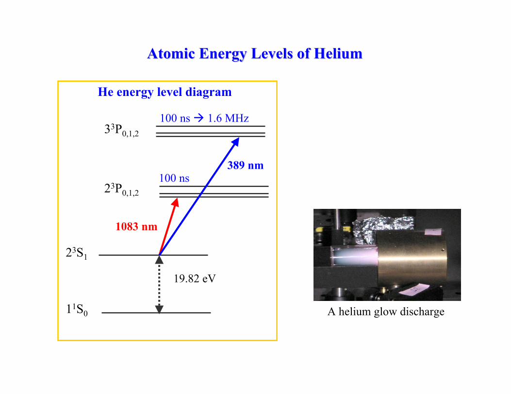
Variational energies for the n = 10 singlet and triplet states of helium.
State Singlet Triplet
10 S –2.005 142 991 747 919(79) –2.005 310 794 915 611 3(11)
10 P –2.004 987 983 802 217 9(26) –2.005 068 805 497 706 7(30)
10 D –2.005 002 071 654 256 81(75) –2.005 002 818 080 228 84(53)
10 F –2.005 000 417 564 668 80(11) –2.005 000 421 686 604 88(26)
10 G –2.005 000 112 764 318 746(22) –2.005 000 112 777 003 317(21)
10 H –2.005 000 039 214 394 532(17) –2.005 000 039 214 417 416(17)
10 I –2.005 000 016 086 516 1947(3) –2.005 000 016 086 516 2194(3)
10 K –2.005 000 007 388 375 8769(0) –2.005 000 007 388 375 8769(0)
E = −2− 1
2n2+ · · ·
= −2.005 · · ·
semin41.tex, January, 2005

ASYMPTOTIC EXPANSIONS
Core Polarization Model (Drachman)
– neglect exchange.
– Rydberg electron moves in the field generated by the polarizable core.
V (x) = − Z − 1
x+ ∆V (x)
pppppp
ppppppp pp pp pp ppppppppppppppp
pp
pp
pp
pp
pp
pp
pp
p
p
p
p
p
p
p
p
p
p
p
p
p
p
p
p
p
p
p
p
p
p
p
p
p
p
p
p
p
p
p
p
p
p
p
p
p
p
p
p
p
p
p
p
p
p
p
p
p
p
p
p
p
p
p
p
p
p
p
p
p
p
p
p
p
p
p
p
p
p
p
p
p
p
p
p
p
p
p
p
p
p
p
p
p
p
p
p
pp
pp
pp
pp
pp
pp
pp
ppppppppppppppp pp pp ppppppp
pppppppppppppppppppppppppppppppptt
pp
ppppppppppppppppppppppppppp
p
p
p
p
p
p
p
p
p
p
p
p
p
p
p
p
p
p
p
p
p
p
p
p
p
p
p
p
p
p
p
p
p
p
p
p
p
p
p
p
p
p
p
p
p
p
p
p
p
p
p
p
p
p
p
p
p
p
p
p
p
p
p
p
p
p
p
p
p
p
p
p
p
p
p
p
p
p
p
p
p
p
p
p
p
p
pp
pp
pp
pp
pp
ppppppp pp ppppppppp
pppppppppppppppppppppppppppppppp
t
»»»»»»9
»»»»»»:
xZe−
Polarizable core
e−
Rydberg electron
Illustration of the physical basis for the asymptotic expansion method in
which the Rydberg electron moves in the field generated by the polarized
core.
∆V (x) = − c4
x4− c6
x6− c7
x7− c8
x8− c9
x9− c10
x10+ · · ·
For example, c4 = 12α1.
semin40.tex, January, 2005

Then
∆EnL = − (Z − 1)2
2n2+ 〈χ0 | ∆V (x) | χ0〉 + 〈χ0 | ∆V (x) | χ1〉
where | χ1〉 = first-order perturbation correction to | χ0〉 due to ∆V (x);
i.e.
[h0(x)− e0] | χ1〉 + ∆V (x) | χ0〉 =| χ0〉〈| ∆V (x) | χ0〉semin40.tex, January, 2005

Asymptotic expansion for the energy of the 1s10k state of helium.
Quantity Value
−Z2/2 –2.000 000 000 000 000 00
−1/(2n2) –0.005 000 000 000 000 00
c4〈r−4〉 –0.000 000 007 393 341 95
c6〈r−6〉 0.000 000 000 004 980 47
c7〈r−7〉 0.000 000 000 000 278 95
c8〈r−8〉 –0.000 000 000 000 224 33
c9〈r−9〉 –0.000 000 000 000 002 25
c10〈r−10〉 0.000 000 000 000 003 73
Second order –0.000 000 000 000 070 91
Total –2.005 000 007 388 376 30(74)
Variational –2.005 000 007 388 375 8769(0)
Difference –0.000 000 000 000 000 42(74)
' 3 Hz
semin42.tex, January, 2005

Two-electron Bethe logs for high angular momentum
β(1snl) = β(1s) +
(Z − 1
Z
)4 β(nl)
n3 +0.316205
Z6 〈x−4〉+ ∆β(1snl)
Residual two-electron Bethe logs n3∆β(1snl).
State n3∆β(1snl) Least squares fit Difference3 1D –0.000 001 08(4)3 3D 0.000 181 74(5)
4 1D –0.000 018 4(3)4 3D 0.000 231 18(7)
5 1D –0.000 026 84(9)5 3D 0.000 249 73(12) a
4 1F 0.000 006 58(2) 0.000 006 60 –0.000 000 02(2)4 3F 0.000 007 63(2) 0.000 007 64 –0.000 000 01(2)
5 1F 0.000 008 70(3) 0.000 008 69 0.000 000 01(3)5 3F 0.000 010 42(3) 0.000 010 41 0.000 000 01(3)
6 1F 0.000 009 8(1) 0.000 009 83 0.000 000 0(1)6 3F 0.000 011 9(3) 0.000 011 98 –0.000 000 1(3)
5 1G 0.000 000 770(3) 0.000 000 770 0.000 000 000(3)5 3G 0.000 000 771(3) 0.000 000 771 0.000 000 000(3)
6 1G 0.000 001 043(3) 0.000 001 042 0.000 000 001(3)6 3G 0.000 001 050(8) 0.000 001 047 0.000 000 003(8)
6 1H 0.000 000 127(2) 0.000 000 127 0.000 000 000(2)6 3H 0.000 000 127(2) 0.000 000 127 0.000 000 000(2)
a Corresponds to an energy uncertainty of ±14 Hz.
A least-squares fit gives
∆β(1snl 1L) = 95.6(0.9)〈x−6〉 − 841(19)〈x−7〉+ 1394(50)〈x−8〉∆β(1snl 3L) = 95.0(0.9)〈x−6〉 − 840(23)〈x−7〉+ 1581(60)〈x−8〉

Partial contributions to the Bethe log for the1s5g 1G state of He.
PartialΩ N Bethe log Difference Ratio
5 1G− n 1F (25.9%)
4 222 4.369 008 35395 353 4.370 451 7910 0.001 443 43726 522 4.370 605 2673 0.000 153 4763 9.4057 688 4.370 622 6186 0.000 017 3513 8.8458 878 4.370 624 3521 0.000 001 7335 10.0099 1105 4.370 624 5545 0.000 000 2023 8.568
10 1399 4.370 624 5749 0.000 000 0204 9.91611 1716 4.370 624 5772 0.000 000 0023 8.836Extrap. 4.370 624 5775 0.000 000 0003
5 1G− n 1Go (33.3%)
4 169 4.370 262 90445 265 4.370 397 1135 0.000 134 20916 385 4.370 411 1743 0.000 014 0608 9.5457 530 4.370 412 7458 0.000 001 5715 8.9478 699 4.370 412 9039 0.000 000 1582 9.9359 894 4.370 412 9227 0.000 000 0187 8.443
10 1126 4.370 412 9247 0.000 000 0020 9.35312 1384 4.370 412 9249 0.000 000 0003 7.664Extrap. 4.370 412 9250 0.000 000 0001
5 1G− n 1H (40.7%)
4 260 4.370 124 59415 403 4.370 283 7562 0.000 159 16216 585 4.370 299 9202 0.000 016 1640 9.8477 806 4.370 301 7021 0.000 001 7818 9.0718 1066 4.370 301 8745 0.000 000 1725 10.3329 1372 4.370 301 8944 0.000 000 0199 8.669
10 1742 4.370 301 8965 0.000 000 0020 9.705Extrap. 4.370 301 8967 0.000 000 0002

Atomic Isotope ShiftAtomic Isotope Shift
Isotope Shift δν = δνMS + δνFS
Field shift:due to nucleus size
δνFS∝ Ζ × ∆[Ψ(0)]2 × δ<r2>
IS(23S1 - 23P2) = 34473.625(20) + 1.210(<r2>He4 - <r2>He6) MHzIS(23S1 - 33P2) = 43196.202(20) + 1.008(<r2>He4 - <r2>He6) MHz*G. Drake, Univ. of Windsor, private communication
100 kHz error in frequency 1% error in radius
δνMS ∝ ''
AAAA−
Mass shift:due to nucleus recoil

Single Atom DetectionSingle Atom Detection
95 100
0
50
100
150
time (sec)
phot
on c
ount
s / 5
0ms
One 4He atom in the trap
Capture efficiency ~ 10-8
Single atom detection necessary!
Single-atom signal ~ 1.5 kHz
Single-atom S/N ~ 10 in 100 ms6He capture rate ~ 100 per hour

NucleonNucleon--Nucleon Interaction at Low EnergyNucleon Interaction at Low Energy
Fundamental theory QCD not calculable in low-energy regime (nucleus structure)
Modern nuclear calculation uses “effective potential” between nucleons
QCD
q
q
NN
N
MesonExchange
π
N

Isotope Shifts and Charge Radius
of Halo Nuclei
Gordon W.F. Drake
University of Windsor and GSI
Collaborators
Zong-Chao Yan (UNB)
Mark Cassar (PDF)
Zheng Zhong (Ph.D. student)
Qixue Wu (Ph.D. student)
Atef Titi (Ph.D. student)
Razvan Nistor (M.Sc. completed)
Levent Inci (M.Sc. completed)
Financial Support: NSERC and SHARCnet
Imperial College, February 27, 2006.
semin00.tex

Main Theme:
• Derive nuclear charge radii by combining atomic theory with high pre-
cision spectroscopy (especially 6He and 11Li halo nuclei).
What’s New?
1. Essentially exact solutions to the quantum mechanical three- and four-
body problems.
2. Recent advances in calculating QED corrections – especially the Bethe
logarithm.
3. Single atom spectroscopy.
semin00.tex, January 2005

dragon.jpg (JPEG Image, 181x250 pixels)
1 of 1 2005-01-31 12:41 AM

Effective Model & Quantum Monte Carlo CalculationEffective Model & Quantum Monte Carlo Calculation
∑ ∑<
+++=i ji
Rijijiji vvvKH πγ
EM 1-π short-range
Coupling parameters fit to NN scattering data
Problem: binding energy of most light nuclei too small
Rijkijkijkijk VVVV ++= ππ 32
Coupling parameters fit to energy levels of light nuclei
S. Pieper and R. Wiringa. Ann. Rev. Nucl. Part. Sci. 51, 53 (2001)
Two-body potentialArgonne V18
Three-body potentialIllinois-2

High precision measurements for lithium.
Group Measurements
NIST (Radziemski et al. [1]) many transitions
York (Van Wijngaarden et al. [2]) 2 2S – 2 2P I.S.
GSI (Bushaw et al. [3]) 2 2S – 3 2S I.S.
GSI (Ewald et al. [4]) 8Li, 9Li I.S.
TRIUMF/GSI (Sanchez et al. [5]) 11Li I.S.
Windsor/UNB (Yan, Drake [6]) theory
[1] L. J. Radziemski, R. Engleman, Jr., and J. W. Brault, Phys. Rev. A 52, 4462 (1995).[2] J. Walls, R, Ashby J.J. Clarke, B. Lu, and W.A. van Wijngaarden, Eur. Phys. J D22 159 (2003).[3] B. A. Bushaw, W. Nortershauser, G. Ewalt, A. Dax, and G. W. F. Drake, Phys.Rev. Lett. 91, 043004 (2003).[4] G. Ewald, W. Nordershauser, A. Dax, S. Gote, R. Kirchner, H.-J. Kluge, Th. Kuhl,R. Sanchez, A. Wojtaszek, B.A. Bushaw, G.W.F. Drake, Z.-C. Yan, and C. Zimmer-mann, Phys. Rev. Lett. 93, 113002 (2004) (2004).[5] R. Sanchez et al. Phys. Rev. Lett. 96, 033022 (2006).[6] Z.-C. Yan and G.W.F. Drake, Phys. Rev. Lett. 91, 113004 (2003).
transp05.tex, Feb., 2006

Comparison of values for the rms nuclear charge radius R of 3He obtainedby various methods. (IS: isotope shift)
Method R (fm) Year Author
e− scattering 1.87(5) 1965 Collard et al.
e− scattering 1.88(5) 1970 McCarthy et al.
e− scattering 1.844(45) 1977 McCarthy et al.
e− scattering 1.89(5) 1977 Szalata et al.
e− scattering 1.935(30) 1983 Dunn et al.
e− scattering 1.877(30) 1984 Retzlaff et al.
e− scattering 1.976(15) 1985 Ottermann et al.
e− scattering 1.959(30)a 1994 Amroun et al.
Theory 1.92 1983 Hadjimichael et al.
Theory 1.92 1986 Schiavilla et al.
Theory 1.93 1986 Chen et al.
Theory 1.95 1987 Strueve et al.
Theory 1.92 1988 Kim et al.
Theory 1.958(6) 1993 Wu et al.
Theory 1.954(7) 1993 Friar et al.
Theory 1.96(1) 2001 Piper and Wiringa
Atomic IS 1.951(10)b 1993 Drake
Atomic IS 1.9659(14) 1994 Shiner et al.
Atomic IS 1.985(42) 1994 Marin et al.
aAnalysis and fit to all previous electron scattering data.bFrom the measurements of Zhao et al., and corrected for hyperfine mixing of the 2 3S1
state with the 2 1S0 state.
transp11.tex, March 99

Comparison of nuclear charge radius determinations for 3He.
rc (fm)
1.85 1.90 1.95 2.00 2.05
oHe(2 3S1 – 2 3P0) IS
oHe(2 3S1 – 2 3P1) IS
oHe(2 3S1 – 2 3P2) IS
oHe(2 3S1 – 2 3P0) IS
oHe(2 3S1 – 3 3P0) IS
xe−-nuclear scattering
INuclear theory
semin20.tex, January, 2005

Comparison of nuclear charge radius determinations for 6Li.
rc (fm)
2.30 2.35 2.40 2.45 2.50 2.55 2.60
oLi+(2 3S1 – 2 3P0) IS
oLi+(2 3S1 – 2 3P1) IS
oLi+(2 3S1 – 2 3P2) IS
oLi(2 2S1/2 – 3 2S1/2) IS
oLi(2 2S1/2 – 3 2S1/2) IS
oLi(2 2S1/2 – 2 2P1/2) IS
oLi(2 2S1/2 – 2 2P1/2) IS
oLi(2 2S1/2 – 2 2P3/2) IS
oLi(2 2S1/2 – 2 2P1/2) IS
oLi(2 2S1/2 – 2 2P3/2) IS
oLi(2 2S1/2 – 2 2P1/2) IS
oLi(2 2S1/2 – 2 2P3/2) IS
xe−-nuclear scattering
INuclear theory
The inner error bars exclude the ±0.03 fm uncertainty due to the reference radiusrc(
7Li) = 2.39(3) fm.
semin21.tex, January, 2005

Strategy
1. Calculate nonrelativistic eigenvalues for helium-like and lithium-like ions to spec-troscopic accuracy.
2. Include finite nuclear mass (mass polarization) effects up to second order by per-turbation theory.
3. Include relativistic and QED corrections by perturbation theory.
4. Compare the results for transition frequencies with high precision measurements.
5. Use the residual discrepancy between theory and experiment to measure the nuclearcharge radius of exotic “halo” isotopes of lithium such as 11Li.
Question: Why not use hydrogenic ions where the theory is much simpler?
Answer: Line widths are narrower in the corresponding helium-like or lithium-like ionby a factor of 100 or more, and these charge states are easier to produce.
semin22.tex, January 2005

Bethe logarithms for lithium
N β(2 2S) Difference Ratio
87 2.846 5271
207 2.964 2629 0.117 7357
459 2.978 9857 0.014 7228 8.00
937 2.980 7196 0.001 7339 8.49
1763 2.980 9043 0.000 1847 9.39
Extrp. 2.980 93(3)
Li+(1s2 1S) 2.982 624 555(4)
N β(3 2S) Difference Ratio
87 2.746 4739
207 2.939 4848 0.193 0108
459 2.975 0774 0.035 5926 5.42
937 2.981 2660 0.006 1886 5.75
1763 2.982 2261 0.000 9601 6.45
Extrp. 2.982 4(2)
Li+(1s2 1S) 2.982 624 555(4)
Z.-C. Yan and G. W. F. Drake, “Bethe logarithm and QED shift for lithium”, Phys.Rev. Lett. 91, 113004 (2003).
semin13.tex, January 2005

Bethe logarithms for lithium – finite mass correction
N ∆βM(2 2S) Difference Ratio
87 0.123 748
207 0.119 291 0.004 457
459 0.115 390 0.003 901 1.14
937 0.114 140 0.001 250 3.12
1763 0.113 845 0.000 295 4.24
Extrap 0.113 5(3)
Li+(1s2 1S) 0.1096
N ∆βM(3 2S) Difference Ratio
87 0.098298281
207 0.104933801
459 0.110410361
937 0.112767733
1763 0.110416727
Extrap 0.112(1)
Li+(1s2 1S) 0.1096
Z.-C. Yan and G. W. F. Drake, “Bethe logarithm and QED shift for lithium”, Phys.Rev. Lett. 91, 113004 (2003).
semin13.tex, January 2005

Final Results for the 6He Isotope Shift
Using the accurately measured transition frequency in 4He as a reference, the transitionfrequency in 6He can be accurately calculated to be
ν(2 3S1 − 2 3P2) = 276 766 663.53(2)− 1.2104r26He MHz (9)
where r6He is the rms nuclear radius of 6He, in units of fm, and the 6He – 4He isotopeshift is
δν(2 3S1 − 2 3P2) = 34 473.625(13) + 1.2104(r24He − r2
6He) MHz . (10)
δν(2 3S1 − 3 3P2) = 43 196.202(16) + 1.008(r24He − r2
6He) MHz . (11)
The uncertainty of ±16 kHz is due entirely to the uncertainty in the measured atomicmass of 6He (6.018 888(1) u), and not to the atomic structure calculations themselves.From Eq. (11) it follows that a measurement of the isotope shift to an accuracy of 100kHz is sufficient to determine the nuclear radius of 6He (relative to 4He) to an accuracyof 1%. The result provides a direct test of the theoretical value r6He = 2.04 fm recentlyobtained by Monte Carlo techniques by
S.C. Pieper, and R.B. Wiringa. Ann. Rev. Nucl. Part. Science 51, 53 (2001); S.C.Pieper, K. Varga, and R.B. Wiringa, Phys. Rev. C 66, 044310 (2002).
Argonne Collaboration L.-B. Wang, P. Mueller, K. Bailey, G.W.F. Drake, J. Greene,D. Henderson, R.J. Holt, R.V.F. Janssens, C.L. Jiang, Z.-T. Lu, T.P. O’Conner, R.C.Pardo, K.E. Rehm, J.P. Schiffer, and X.-D. Tang.
semin17.tex, June, 2004

Single AtomSingle AtomSpectroscopySpectroscopy
~ 150 6He atoms in one hour
April 6, 2004
-8 -6 -4 -2 0 2 4 6 80
200
400
600
800
1000
1200 xc: 0.034 +/- 0.030 MHzw: 5.737 +/- 0.095 MHz
phot
on c
ount
sfrequency (MHz)
-8 -6 -4 -2 0 2 4 6 850
100
150
200
250
300xc: -0.008 +/- 0.106 MHzw: 5.135 +/- 0.298 MHz
frequency (MHz)
phot
on c
ount
s
4He
6He

658.5 659.0
Lamb ('57)
Pipkin ('78)
Metcalf ('86)
ATTA ('04)
8113.5 8114.0 8772.0 8772.5
3 3P1 - 3 3P
2
3 3P
0 - 3 3P1
3 3P0 - 3 3P
2
4He Finestructure Splitting in 3p 3P0,1,2
FS Splitting in MHzLamb ('57): I. Wieder and W.E. Lamb, Jr., Phys. Rev. 107, 125 (1957)Pipkin ('78): P. Kramer and F. Pipkin, Phys. Rev. A18, 212 (1978)Metcalf ('86): D.-H. Yang, P. McNicholl, and H. Metcalf, Phys. Rev. A33, 1725 (1986)ATTA ('04): this work Drake ('04): private ommuncation

658.5 659.0
Lamb ('57)
Pipkin ('78)
Metcalf ('86)
ATTA ('04)
Drake ('04)
8113.5 8114.0 8772.0 8772.5
3 3P1 - 3 3P23 3P0 - 3 3P1
3 3P0 - 3 3P2
4He Finestructure Splitting in 3p 3P0,1,2
FS Splitting in MHzLamb ('57): I. Wieder and W.E. Lamb, Jr., Phys. Rev. 107, 125 (1957)Pipkin ('78): P. Kramer and F. Pipkin, Phys. Rev. A18, 212 (1978)Metcalf ('86): D.-H. Yang, P. McNicholl, and H. Metcalf, Phys. Rev. A33, 1725 (1986)ATTA ('04): this work Drake ('04): private ommuncation

Experimental Setup Experimental Setup -- SchematicSchematic
Transport time ~ 1 sec
PhotonCounter
RF dischargeKr, 4He
6HeHe* Zeeman Slower MOT
TransversalCooling
389 nm 1083 nm
6HeProduction
Kr or 4HeCarrier gas
Mixingchamber
389 nm
2S-2P, 1083 nm
2S-3P, 389 nm

Experimental Setup Experimental Setup -- SchematicSchematic
Transport time ~ 1 sec
PhotonCounter
RF dischargeKr, 4He
6HeHe* Zeeman Slower MOT
TransversalCooling
389 nm 1083 nm
6HeProduction
Kr or 4HeCarrier gas
Mixingchamber
389 nm
2S-2P, 1083 nm
2S-3P, 389 nm

Two-Photon Lithium Spectroscopy
LiS
Experimental Arrangement
Ti:Sa Laser735 nm
Dye Laser 610 nm
ElectrostaticLenses
PZT
CO -Laser2
Comparison
Serv
o
RF Generator
Reference Diode Laser I2
Servo
UNILAC BeamC, 11.4 MeV/u12
Reaction Products
Surface Ion Source
Magnet
Servo
Servo
W Target
Ion Signal

6He - Nuclear Charge Radius
Isotope shift(23S1 - 33P2, 6He – 4He)
43 194.772(56) MHz
6He rms charge radius
2.054(14) fm (0.7%)
L.-B. Wang et al.,PRL 93, 142501 (2004)
1.7 1.8 1.9 2.0 2.1 Point-Proton Radius of He-6 (fm)
He-6
Reaction collision
Elastic collision
Atomic isotope shift
Cluster models
No-core shell model
Quantum MC
Modelindependent!
Expe
rimen
tTh
eory
Tanihata ‘92
Alkhazov ‘97
This work
Csoto ‘93
Funada ‘94
Varga ‘94
Wurzer ‘97
Esbensen ‘97
Navratil ‘01
Pieper ‘04
Courtesy of Peter Müller, Argonne Nat. Lab

Determination of the Nuclear Radius for Isotopes of Lithium
R2rms(
ALi) = R2rms(
6Li) +EA
meas − EA0
C(12)
where EAmeas is the measured isotope shift for ALi relative to 6Li, and EA
0
contains all the calculated contributions to the isotope shift with the excep-
tion of the shift due to finite nuclear size.
Values of EA0 to determine R2
rms from the
measured isotope shift in various transitions. Units are MHz.
Isotopes EA0 (2 2P1/2 − 2 2S) EA
0 (2 2P3/2 − 2 2S) EA0 (3 2S − 2 2S)
7Li–6Li 10 532.19(7) 10 532.58(7) 11 453.00(6)8Li–6Li 18 472.86(12) 18 473.55(12) 20 088.10(10)9Li–6Li 24 631.11(16) 24 632.03(16) 26 785.01(13)10Li–6Li 29 575.46(20) 29 576.56(20) 32 161.92(17)11Li–6Li 33 615.19(24) 33 616.45(24) 36 555.11(21)
C = −2.4565 MHz/fm2 for the 2 2PJ − 2 2S1/2 I.S.
C = −1.5661 MHz/fm2 for 3 2S1/2 − 2 2S1/2 I.S.

Contributions to the 7Li 1s23s 2S− 1s22s 2S transition energyand 1s22s 2S ionization potential (I.P.), in units of cm−1.
Term 3 2S1/2 − 2 2S1/2 2 2S1/2 I.P.
Nonrelativistic 27 206.492 856(4) 43 488.220 2449(16)Nonrel., µ/M –2.295 854 30(16) –3.621 707 668(4)Nonrel., (µ/M)2 0.000 165 962 0.000 315 803Relativistic, α2 2.089 0(4) 2.811 33(2)Rel. recoil, α2µ/M –0.000 04(1) –0.000 011(9)QED(e−–nucl.), α3 –0.198 6(3) –0.258 32(3)QED(e−–e−), α3 0.010 747 0.013 884QED higher order, α4 · · · –0.005 4(4) –0.007 0(4)Nuclear size, R2 –0.000 298(8) –0.000 389(10)Total 27 206.092 6(9) 43 487.158 3(6)Expt. 27 206.095 2(10)a 43 487.150(5)c
27 206.094 20(9)b 43 487.159 34(17)d
Diff. –0.001 6(9) –0.001 0(5)
aL. J. Radziemski, R. Engleman, Jr., and J. W. Brault, Phys. Rev. A 52, 4462 (1995).bB. A. Bushaw, W. Nortershauser, G. Ewalt, A. Dax, and G. W. F. Drake, Phys. Rev.Lett. 91, 043004 (2003).
cC. E. Moore, NSRDS-NBS Vol. 14 (U.S. Department of Commerce, Washington, DC,1970.
dBruce Bushaw, preliminary value.
semin25.tex, January 2005

Contributions to the 7Li–6Li isotope shifts for the 1s22p 2PJ–1s22s 2S tran-sitions and comparison with experiment. Units are MHz.
Contribution 2 2P1/2–2 2S 2 2P3/2–2 2S
Theory
µ/M 10 533.501 92(60)a 10 533.501 92(60)a
(µ/M)2 0.057 3(20) 0.057 3(20)
α2 µ/M –1.397(66) –1.004(66)
α3 µ/M , anom. magnetic –0.000 175 3(84) 0.000 087 5(84)
α3 µ/M , one-electron 0.0045(10) 0.0045(10)
α3 µ/M , two-electron 0.010 5(20) 0.010 5(20)
r2rms 1.94(61) 1.94(61)
r2rms µ/M –0.000 73(11) –0.000 73(11)
Total 10 534.12(7)±0.61 10 534.51(7)±0.61
Experiment
Sansonetti et al.b 10 532.9(6) 10 533.3(5)
Windholz et al.c 10 534.3(3) 10 539.9(1.2)
Scherf et al.d 10 533.13(15) 10 534.93(15)
Walls et al.e 10 534.26(13)
aThe additional uncertainty from the atomic mass determinations is ±0.008 MHz.bC. J. Sansonetti, B. Richou, R. Engleman, Jr., and L. J. Radziemski, Phys. Rev. A 52,2682 (1995).
cL. Windholz and C. Umfer, Z. Phys. D 29, 121 (1994).dW. Scherf, O. Khait, H. Jager, and L. Windholz, Z. Phys. D 36, 31, (1996).eJ. Walls, R. Ashby, J. J. Clarke, B. Lu, and W. A. van Wijngaarden, Eur. Phys. J D22 159 (2003).
semin15.tex, June, 2003

Rayleigh-Schrodinger Variational Principle
Diagonalize H in the
χijk = ri1r
j2r
k12 e−αr1−βr2 YM
l1l2L(r1, r2)
basis set to satisfy the variational condition
δ∫
Ψ (H − E) Ψ dτ = 0.
For finite nuclear mass M ,
H = −1
2∇2
1 −1
2∇2
2 −Z
r1− Z
r2+
1
r12− µ
M∇1 · ∇2
in reduced mass atomic units e2/aµ, where aµ = (m/µ)a0 is the reduced
mass Bohr radius, and µ = mM/(m + M) is the electron reduced mass.
transp09.tex, January/05

Rescale distances and energies according to
ρ = r/aµ
E = E/(e2/aµ)
where aµ =h2
µe2is the reduced mass Bohr radius,
ande2
aµ= 2Rµ = 2
µ
mR∞ = 2
(1− µ
M
)R∞.
The Schrodinger equation is then (in mass-scaled atomic units)−
1
2∇2
ρ1− 1
2∇2
ρ2− µ
M∇ρ1 · ∇ρ2 −
Z
ρ1− Z
ρ2+
1
|ρ1 − ρ2|
Ψ = EΨ
semin03.tex, January/05

New Variational Techniques
I. Double the basis set
If φi,j,k(α, β) = ri1r
j2r
k12e
−αr1−βr2
then φi,j,k = a1φi,j,k(α1, β1) + a2φi,j,k(α2, β2)
asymptotic inner correlation
II. Include the screened hydrogenic function
φSH = ψ1s(Z)ψnL(Z − 1)
explicitly in the basis set.
III. Optimize the nonlinear parameters
∂E
∂αt= −2〈Ψtr | H − E | r1Ψ(r1, r2; αt)± r2Ψ(r2, r1; αt)〉
∂E
∂βt= −2〈Ψtr | H − E | r2Ψ(r1, r2; αt)± r1Ψ(r2, r1; αt)〉
for t = 1, 2, with 〈Ψtr | Ψtr〉 = 1.
Ψ(r1, r2; αt) = terms in Ψtr which depend explicitly on αt.
semin04.tex, January, 2005

Convergence of the nonrelativistic energies for the 1s22s 2S and 1s22p 2Pstates of lithium, in atomic units.
Ω No. of terms E(Ω) E(Ω)− E(Ω− 1) R(Ω)a
1s22s 2S
2 19 –7.477 555 720 321 83 51 –7.477 995 835 140 8 –0.000 440 114 819 04 121 –7.478 053 567 299 9 –0.000 057 732 159 1 7.6235 257 –7.478 059 464 463 7 –0.000 005 897 163 8 9.7906 503 –7.478 060 228 080 1 –0.000 000 763 616 4 7.7237 919 –7.478 060 311 092 9 –0.000 000 083 012 9 9.1998 1590 –7.478 060 321 724 7 –0.000 000 010 631 8 7.8089 2626 –7.478 060 323 416 8 –0.000 000 001 692 1 6.28310 3502 –7.478 060 323 618 9 –0.000 000 000 202 1 8.371∞ –7.478 060 323 650 3(71)
1s22p 2P2 20 –7.410 088 210 4273 56 –7.410 146 240 952 –0.000 058 030 5254 139 –7.410 155 057 909 –0.000 008 816 956 6.5825 307 –7.410 156 274 821 –0.000 001 216 912 7.2456 623 –7.410 156 490 483 –0.000 000 215 662 5.6437 1175 –7.410 156 524 272 –0.000 000 033 789 6.3838 1846 –7.410 156 530 070 –0.000 000 005 798 5.8289 2882 –7.410 156 531 534 –0.000 000 001 464 3.96010 3463 –7.410 156 531 721 –0.000 000 000 187 7.813∞ –7.410 156 531 763(42)
aR(Ω) =R(Ω− 1)−R(Ω− 2)
R(Ω)−R(Ω− 1)semin06.tex, January, 2005

QED Corrections
the QED shift for a 1s2nL n 2L state of lithium then has the form
EQED = EL,1 + EM,1 + ER,1 + EL,2
where the main one-electron part is (in atomic units)
EL,1 =4Zα3〈δ(ri)〉(0)
3
ln(Zα)−2 − β(n 2L) +
19
30+ · · ·
the mass scaling and mass polarization corrections are
EM,1 =µ〈δ(ri)〉(1)
M〈δ(ri)〉(0)EL,1 +4Zα3µ〈δ(ri)〉(0)
3M
[1−∆βMP(n 2L)
]
and the recoil corrections (including radiative recoil) are given by
ER,1 =4Z2µα3〈δ(ri)〉(0)
3M
[1
4ln(Zα)−2 − 2β(n 2L)− 1
12− 7
4a(n 2L)
]
where β(n 2L) = ln(k0/Z2R∞) is the two-electron Bethe logarithm.
semin08.tex, January, 2005
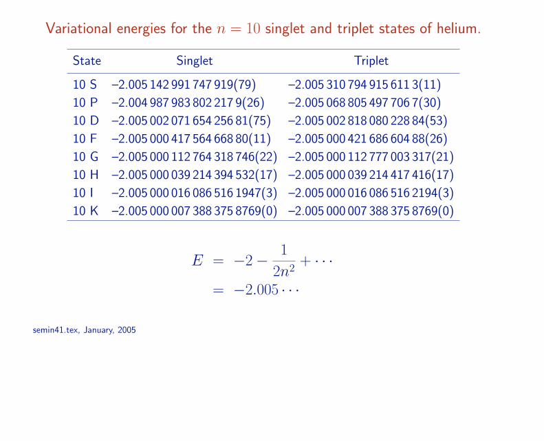
The Recoil Term
The recoil term a(n 2L) corresponds, in the hydrogenic case, to the term a(nL) givenby
a(nL) = −2
ln
2
n+
n∑
q=1q−1 + 1− 1
2n
δL,0 +
1− δL,0
L(L + 1)(2L + 1). (4)
In the multi-electron case, it corresponds to the term
a(n 2L) =2Q1
〈δ(ri)〉(0) + 2 ln Z − 3 . (5)
where Q1 is the matrix element
Q1 = (1/4π) limε→0〈r−3
i (ε) + 4π(γeu + ln ε)δ(ri)〉 ,
γeu is Euler’s constant, ε is the radius of a sphere about ri = 0 excluded from theintegration, and a summation over i from 1 to 3 is assumed for lithium.
semin08.tex, January, 2005

Variational upper bounds for nonrelativistic eigenvalues.
State Nterms E∞ (2R∞) EM (2RM)
Li(1s22s 2S) 6413 –7.478 060 323 869 –7.478 036 728 322
9577 –7.478 060 323 892 –7.478 036 728 344
Li(1s23s 2S) 6413 –7.354 098 421 392 –7.354 075 591 755
9577 –7.354 098 421 425 –7.354 075 591 788
Li(1s22p 2P ) 5762 –7.410 156 532 488 –7.410 137 246 549
9038 –7.410 156 532 593 –7.410 137 246 663
Be+(1s22s 2S) 6413 –14.324 763 176 735 –14.324 735 613 884
9577 –14.324 763 176 767 –14.324 735 613 915
Be+(1s23s 2S) 6413 –13.922 789 268 430 –13.922 763 157 509
9577 –13.922 789 268 518 –13.922 763 157 598
Be+(1s22p 2S) 5762 –14.179 333 293 227 –14.179 323 188 964
9038 –14.179 333 293 333 –14.179 323 189 509

e The Electron-Electron Term
The electron-electron part is (Araki and Sucher)
∆EL,2 = α3(14
3ln α +
164
15
)〈δ(rij)〉 − 14
3α3Q , (6)
where the Q term is defined by
Q = (1/4π) limε→0〈r−3
ij (ε) + 4π(γ + ln ε)δ(rij)〉 . (7)
γ is Euler’s constant, ε is the radius of a sphere about rij = 0 excluded from theintegration.
Finite Nuclear Size Correction
In lowest order
∆Enuc =2πZr2
rms
3〈δ(ri)〉 , (8)
where rrms = Rrms/aBohr, Rrms is the root-mean-square radius of the nuclear chargedistribution, and aBohr is the Bohr radius.
semin08.tex, January, 2005

The sum in the denominator can be completed by closure:
D = 〈Ψ0|p(H − E0)p|Ψ0〉 = 2πZ|Ψ0(0)|2
where p = p1 + p2.
Schwartz (1961) transformed the numerator to read
N = limK→∞
(−K〈Ψ0|p · p|Ψ0〉+D ln(K) +
∫ K
0k dk〈Ψ0|p(H − E0 + k)−1p|Ψ0〉
)
Expensive in computer time and slowly convergent. Recent work by
J. D. Baker,R. C. Rorrrey, M. Jerziorska, and J. D. Morgan III (unpublished),V. I. Korobov and S. V. Korobov, Phys. Rev. A 59, 3394 (1999).
semin09.tex, January, 2005

E (a.u.)
β(E
)
100 102 104 106
0.0
0.5
1.0
1.5
2.0
qq q q q q qqqqqqqqqqqqqqqqqqqqqqqqqqqqqqqqqqqqqqqqqqqqqqqqqqqqqqqqqqqqqqqqqqqqqqqqqqqqqqqqqqqqqqqqqqqqqqqqqqqqqqqqqqqqqqqqqqqqqqqqqqqqqqqqqqqqqqqqqqqqqqqqqqqqqqqqqqqqqqqqqqqqqqqqqqqqqqqqqqqqqqqqqqqqqqqqqq
qqqqqqqqqqqqqqqqqqqqqqqqqqqqqqqqqqqqqqqqqqqqqqqqqqqqqqqqqqqqqqqqqqqqqqqqqqqqqqqqqqqqqqqqqqqqqqqqqqqqqqqqqqqqqqqqqqqqqqqqqqqqqqqqqqqqqqqqqqqqqqqqqqqqqqqqqqqqqqqqqqqqqqqqqqqqqqqqqqqqqqqqqqqqqqqqqqqqqqqqqqqqqqq
qqqqqqqqqqqqqqqqqqqqqqqqqqqqqqqqqqqqqqqqqqqqqqqqqqqqqqqqqqqqqqqqqqq
qqqqqqqqqqqqqqqqqqqqqqqqqqqqqqqqqqqqqqqqqqqqqqqqqqqqqqqqqqqqqqqqqqqqqqqqqqqqqqqqqqqqqqqqqqqqqqqqqqqqqqqqqqqqqqqqqqqqqqqqqqqqqqqqqqqqqqqqqqqq
qqqqqqqqqqqqqqqqqqqqqqqqqqqqqqqqqqqqqqqqqqqqqqqqqqqqqqqqqqqqqqqqqqqqqqqqqqqqqqqqqqqqqqqqqqqqqqqqqqqqqqqqqqqqqqqqqqqqqqqqqqqqqqqqqqqqqqqqq
qqqqqqqqqqqqqqqqqqqqqqqqqqqqqqqqqqqqqqqqqqqqqqqqqqqqqqqqqqqqqqqqqqqqqqqqqqqqqqq
qqqqqqqqqqqqqqqqqqqqqqqqqqqqqqqqqqqqqqqqqqqqqqqqqqqqqqqqqqqq
qqqqqqqqqqqqqqqqqqqqqqqqqqqqqqqqqqqqqqqqqqqqqqqqqqqqqqqqqqqqqqqqqqqqqqqqqqqqqqqqqqqqqqqqqqqqqqqqqqq
qqqqqqqqqqqqqqqqqqqqqqqqqqqqqqqqqqqqqqqqqqqqqqqqqqqqqqqqqqqqq
qqqqqqqqqqqqqqqqqqqqqqqqqqqqqqqqqqqqqqqqqqq
qqqqqqqqqqqqqqqqqqqqqqqqqqqqqq
q qqqqqqqqqqqqqqq qqqqq qqqq qqqqqq
q qqqqqqqqq q qqq q qqqqqqqqqqq qqqq q qqqq q
eeeeeeeeeeeeeeeeeee
ee
eeeeeeeeeeeee
ee
ee
eeeeeeeeeeeeeeeeeeeeeeeeee
Partial Bethe logarithm sums for the ground state of helium, summed over pseudostatesup to energy E. Each solid point represents the contribution from one pseudostate.The open circles are the corresponding partial sums for hydrogen.
semin11.tex, January, 2005
CE: PM
INSTITUTE OF PHYSICS PUBLISHING JOURNAL OF PHYSICS B: ATOMIC, MOLECULAR AND OPTICAL PHYSICS
J. Phys. B: At. Mol. Opt. Phys. 37 (2004) 1–8 PII: S0953-4075(04)71603-X
High precision variational calculations for H+2
Mark M Cassar and G W F Drake
University of Windsor, Windsor, ON N9B 3P4, Canada
E-mail: [email protected]
Received 5 November 2003, in final form 29 April 2004Published DD MMM 2004Online at stacks.iop.org/JPhysB/37/1DOI: 10.1088/0953-4075/37/0/000
AbstractA double basis set in Hylleraas coordinates is used to obtain improvedvariational upper bounds for the nonrelativistic energy of the 1 1S (v = 0, R =0), 2 1S (v = 1, R = 0) and 2 3P (v = 0, R = 1) states of H+
2. Thismethod shows a remarkable convergence rate for relatively compact basis setexpansions. A comparison with the most recent work is made. The accuracyof the wavefunctions is tested using the electron–proton Kato cusp condition.
1. Introduction
The hydrogen molecular ion H+2 is a fundamental three-body quantum system. This ion
presents the complexities associated with multi-centred systems while still remaining amenableto high precision calculation. The recent theoretical and experimental interest in this ion comesfrom two fronts. The first is due to the precision measurement of the dipole polarizability forH+
2, as determined by an analysis of the Rydberg states of H2, by Jacobson et al [1, 2]. Thisexperiment revealed a discrepancy with theory of about 0.0007 a3
0 , where a0 is the first Bohrradius. This discrepancy was only partially removed by including the Breit α2 corrections tothe nonrelativistic Hamiltonian [3], where α ≈ 137−1 is the fine structure constant. Thereare, in addition, other unexplained experimental results [4, 5] that would benefit from furthertheoretical study. The second is due to the possible improvement in the accuracy of the protonto electron mass ratio by an order of magnitude. The possibility of a precise determinationof this fundamental mass ratio through the use of two-photon high resolution spectroscopyin H+
2 was pointed out almost a decade ago [6]. In order for such an experiment to be usedfor metrological purposes, however, the relativistic and QED corrections to the energy levelsinvolved in the measured transition frequencies must be known to order α5, in atomic units.The feasibility of this experiment was recently shown by Hilico et al [7], and is currently beingcarried out [8].
The motivation for the present work lies in the fact that if corrections to the nonrelativisticenergy levels of H+
2 are required to order α5 ≈ 10−10, then the wavefunctions must beaccurate, at least, to this same level. The wavefunctions, however, are typically accurate to
0953-4075/04/000001+08$30.00 © 2004 IOP Publishing Ltd Printed in the UK 1

2 M M Cassar and G W F Drake
less than half as many significant figures as the energy; hence, relativistic and QED correctionscalculated from these wavefunctions suffer the same reduction in accuracy. This implies thatthe nonrelativistic energies need to be accurate to order 10−20 or better in order to take fulladvantage of the experimental accuracy.
To date, the most accurate calculations for H+2 have employed two types of basis set
expansions [9–11]. In the first approach, the trial function is expanded in the form
(r1, r2) =n∑
i=1
ai exp(−αir1 − βir2 − γir12) ± (exchange), (1)
where rj is the distance of the electron from the j th proton, r12 is the inter-protonic coordinateand αi , βi and γi are real (or complex) numbers chosen in a so-called quasi-random mannerfrom a small number of real intervals. This method, as described in [9, 10, 12], has yieldedvery accurate upper bounds for the ground state energy and geometrical properties for a widevariety of three-body systems.
In the second approach, the trial function is expanded in Hylleraas coordinates as
(r1, r2) =m∑
q=1
i+j+k∑
i,j,k
a(q)
ijk ri1r
j
2 rk12 exp(−α(q)r1 − β(q)r2) ± (exchange), (2)
where jmin ≈ 35, and q is an integer that partitions the basis set into m sectors withdistinct scale factors α(q) and β(q). In such a calculation, a complete optimization is performedwith respect to all nonlinear parameters. This method yielded an upper bound to the groundstate energy comparable to expansion (1), but with half as many terms, as well as a new upperbound to the first triplet P-state [11].
The present paper extends previous results for H− and Ps− [13], using a double basisset [14], to cover a wider range of bound three-body systems, including H+
2. It was foundthat including higher powers of r12 and an extra exponential scale factor exp(−γ r12) wasessential, since this allows the vibrational modes along the inter-protonic coordinate to be wellrepresented. The result is a new lowest upper bound for the first three states of H+
2, i.e. the(v = 0, R = 0), (v = 0, R = 1) and (v = 1, R = 0) vibronic states (see table 1 of [15] for adiscussion of the correspondence between atomic and molecular notation).
2. Calculations
After isolating the centre-of-mass motion, the Hamiltonian for H+2 may be written (in reduced
mass atomic units) as
H = −1
2∇2
r1− 1
2∇2
r2− µ
me∇r1 · ∇r2 − 1
r1− 1
r2+
1
r12, (3)
where µ is the reduced electron mass; the electron has been chosen to be at the origin of thecoordinate system. The main task now is to solve the Schrodinger equation
H(r1, r2) = E(r1, r2), (4)
for the stationary states of the Hamiltonian H.For our modified double basis set, the trial function for S-states is given by
S(r1, r2) =2∑
p=1
1∑
i,j=0
high∑
k=low
a(p)
ijk ri1r
j
2 rk12 exp(−α(p)r1 − β(p)r2 − γ (p)r12) ± (exchange),
(5)

High precision variational calculations for H+2 3
where 1 i + j , that is, 1 is the maximum sum of powers of r1 and r2,
low = M − 1 + (i + j),
high = M + 1 − (i + j),
and the integer M > 1 is an adjustable parameter; and for states with L > 0,
L>0(r1, r2) =∑
ang
S(r1, r2)YLMl1l2
(r1, r2), (6)
where YLMl1l2
(r1, r2) is a vector-coupled product of spherical harmonics [16] and∑
ang meansthat all distinct angular couplings are included according to the scheme in [17].
Normally, all distinct combinations of powers i, j, k would be included in expansions (5)and (6); however, in order to avoid problems of near linear dependence for S-states, all termswith i > j are omitted only in (5). In addition, we employed a form of truncation firstintroduced by Kono and Hattori [18] in which terms with i+j +|M−k|−|l1−l2|+|j −i| > 1
are avoided.For a given state, M is varied until a minimum in the energy is found for the largest basis
set used. The value of M is then held at this value for all basis set sizes N as 1 is increased.The inclusion of rk
12 exp(−γ r12) in (5) and (6), where k is a large integer, allows the trialfunctions to effectively represent a nuclear vibrational wavefunction, which is known from theBorn–Oppenheimer approximation to be Gaussian [19, 20]. The condition γ ≈ M/2 of [19]naturally appears in this calculation upon optimization of E with respect to γ . It was foundthat M = 39, 38, 37 give the minimum energy (and good convergence) for the three loweststates of H+
2.After constructing the basis set, the principal computational step is to solve the generalized
eigenvalue problem (H − EO)x = 0. The Hamiltonian matrix H and the overlap matrix Ohave elements Hab = 〈φa|H |φb〉, and Oab = 〈φa|φb〉, respectively, where
φ = ri1r
j
2 rk12 exp(−αr1 − βr2 − γ r12), (7)
is any member of the basis set, and a (and b) represents a specific combination of radial powersi, j, k.
The optimization of α(p), β(p) and γ (p) is accomplished by simultaneously calculatingthe first derivatives of the energy with respect to the nonlinear parameters:
∂E
∂α(p)= −2
〈|(H − E)r1|(p)〉〈|〉 , (8)
where (p) denotes the part of the wavefunction that depends explicitly on α(p), and similarlyfor the β(p) and γ (p) derivatives. There is no contribution to these derivatives from variationsof the a
(p)
ijk because of the variational stability of the wavefunction. The final step is then tochange α(p), β(p) and γ (p) in the directions indicated by the derivatives, resolve the generalizedeigenvalue problem, recalculate the derivatives and locate their zeros by Newton’s method.
All calculations were done in quadruple precision (about 32 decimal digits) arithmetic onSHARCnet’s Tiger cluster of Compaq Alpha ES40 workstations.
3. Results
We present our results in tables 1–5. The value used for the proton mass was mp =1836.152 701 [21], in atomic units1. Tables 1, 3 and 4 show the convergence pattern for
1 In order to facilitate a comparison with other results, the more recent value of mp = 1836.152 672 61 [22] was notused.

4 M M Cassar and G W F Drake
Table 1. Convergence study for the ground state of H+2 . (=M + 1) is the highest power of r12
and N is the total number of terms in the basis set. Atomic units are used.
N E() Ratioa
42 33 −0.597 138 979 257 696 807 296 09543 57 −0.597 139 061 191 160 229 487 98244 90 −0.597 139 062 954 250 154 856 869 46.4745 134 −0.597 139 063 120 531 138 258 260 10.6046 190 −0.597 139 063 123 316 985 447 178 59.6947 260 −0.597 139 063 123 402 568 522 508 32.5548 345 −0.597 139 063 123 404 987 310 249 35.3849 447 −0.597 139 063 123 405 072 038 078 28.5550 567 −0.597 139 063 123 405 074 674 920 32.1351 707 −0.597 139 063 123 405 074 825 966 17.4652 868 −0.597 139 063 123 405 074 834 205 18.3353 1052 −0.597 139 063 123 405 074 834 331 65.43
Extrapolation −0.597 139 063 123 405 074 834 338(3) 19.80b 2200 −0.597 139 063 123 405 0740c −0.597 139 063 123 405 076(2)d 3500 −0.597 139 063 123 405 074 83e 1330 −0.597 139 063 123 405 0741f −0.597 139 063 123 405 074 5(4)
a Ratio is the ratio of successive differences [E( − 1) − E( − 2)]/[E() − E( − 1)].b Korobov variational bound [10].c Korobov extrapolation [10].d Bailey and Frolov variational bound [9].e Yan et al variational bound [11].f Yan et al extrapolation [11].
the ground state and the first two excited states of H+2 and comparisons with other calculations.
The ratios given in the last column of each table are defined by
R() = E( − 1) − E( − 2)
E() − E( − 1), (9)
where = M + 1, and thus give the values of the ratios of successive differences in theenergies. If R() were constant, the extrapolated value of the energy would simply be theseries limit of a geometric series. Since this is not the case, we fit the ratios to the forma/b and sum the series of differences to obtain the extrapolated value. The final quoteduncertainty is thus determined from the uncertainty in the parameters a and b. For the threestates calculated, the largest basis set gives the lowest upper bound to date. However, all theresults agree to within their estimated uncertainties.
The wavefunction for each state may be reproduced immediately using the optimized scalefactors listed in table 5. Carrying out a complete optimization of all nonlinear parametersnaturally partitions the basis set into two distinct sectors: one describing the asymptoticbehaviour of the wavefunction, and the other describing the short-range behaviour. Thispartitioning preserves the numerical stability of the calculations within standard quadrupleprecision arithmetic for the basis set sizes listed.
A useful test of the accuracy of the wavefunctions near a two-particle coalescence pointis the Kato cusp condition [23, 24]
νij =⟨δ(rij ) · ∂
∂rij
⟩
〈δ(rij )〉 , (10)

High precision variational calculations for H+2 5
Table 2. Convergence study for the electron–proton cusp condition νep for the 1 1S and 2 1S statesin atomic units.
1 1S 2 1S
N a νep N νep
33 −1.000 019 529 846 20 −1.004 119 449 15057 −0.999 672 587 190 40 −1.001 983 322 00490 −0.999 487 499 090 70 −0.999 731 407 353
134 −0.999 469 240 363 112 −0.999 540 780 459190 −0.999 459 218 417 168 −0.999 467 185 612260 −0.999 456 326 808 240 −0.999 459 647 216345 −0.999 455 752 544 330 −0.999 456 274 413447 −0.999 455 687 556 440 −0.999 455 794 843567 −0.999 455 684 622 572 −0.999 455 713 857707 −0.999 455 679 856 728 −0.999 455 686 394868 −0.999 455 679 492 910 −0.999 455 681 786987 −0.999 455 679 464 1015 −0.999 455 679 820
1240 −0.999 455 679 5021496 −0.999 455 679 491
νbep −0.999 455 679 432 νb
ep −0.999 455 679 432
a Using M = 40 in expansion (5).b Exact value as given by equation (13).
Table 3. Convergence study for the 21S state of H+2 . (=M + 1) is the highest power of r12
and N is the total number of terms in the basis set. Atomic units are used.
N E() Ratioa
39 20 −0.587 151 043 016 274 880 16740 40 −0.587 155 435 230 538 473 19041 70 −0.587 155 671 003 177 129 307 18.6342 112 −0.587 155 678 540 275 385 079 31.2843 168 −0.587 155 679 208 721 236 702 11.2844 240 −0.587 155 679 212 575 658 166 173.4245 330 −0.587 155 679 212 741 279 834 23.2746 440 −0.587 155 679 212 746 648 696 30.8547 572 −0.587 155 679 212 746 807 755 33.7548 728 −0.587 155 679 212 746 811 406 43.5649 910 −0.587 155 679 212 746 812 118 5.1350 1015 −0.587 155 679 212 746 812 191 9.6551 1240 −0.587 155 679 212 746 812 205 5.5752 1496 −0.587 155 679 212 746 812 211 2.03
Extrapolation −0.587 155 679 212 746 812 212(2) 6.18b −0.587 155 679 212(1)c −0.587 155 679 2127d −0.587 155 679 213 6(5)
a Ratio is the ratio of successive differences [E( − 1) − E( − 2)]/[E() − E( − 1)].b Hilico et al [15].c Moss variational bound [26].d Taylor et al [27].
where rij is any inter-particle coordinate. The exact values of the cusps are known to be
νexactij = qiqj
mimj
mi + mj
, (11)

6 M M Cassar and G W F Drake
Table 4. Convergence study for the 23P state of H+2 . (=M + 1) is the highest power of r12
and N is the total number of terms in the basis set. Atomic units are used.
N E() Ratioa
40 39 −0.596 872 821 718 250 761 3141 82 −0.596 873 728 191 903 938 7442 149 −0.596 873 738 113 177 432 23 91.3743 244 −0.596 873 738 822 338 108 35 13.9944 373 −0.596 873 738 832 029 635 19 73.1745 540 −0.596 873 738 832 750 200 25 13.4546 751 −0.596 873 738 832 762 355 10 59.2847 1010 −0.596 873 738 832 764 668 79 5.2548 1323 −0.596 873 738 832 764 729 56 38.0749 1694 −0.596 873 738 832 764 734 80 11.60
Extrapolation −0.596 873 738 832 764 734 96(5) 32.92b −0.596 873 738 832 8(5)c −0.596 873 738 832 8d −0.596 873 738 832 764 733(1)
a Ratio is the ratio of successive differences [E( − 1) − E( − 2)]/[E() − E( − 1)].b Taylor et al [27].c Moss variational bound [26].d Yan et al extrapolation [11].
where qi and qj are the charges and mi and mj are the masses of the particles. In the chosencoordinate system, and in atomic units, the electron–proton cusp is
νep =⟨δ(r1) · ∂
∂r1
⟩
〈δ(r1)〉 , (12)
with the exact value
νexactep = − mp
mp + 1= −0.999 455 679 432 931. (13)
The results of this calculation are shown in table 2.
4. Discussion
The results of this paper demonstrate that a double basis set in Hylleraas coordinates can beeasily constructed to give highly accurate nonrelativistic energies for H+
2. Compared withother methods, this approach produces lower upper bounds using basis sets with fewer or thesame number of terms. For the basis set sizes presented here, the numerical stability of thecalculation is excellent, and so does not require the use of extended precision arithmetic.
One notable feature of this calculation is the large values and scatter of the Ratio, especiallyfor the 2 1S state, given in the last column of tables 1, 3 and 4. Although this would normallyreduce the confidence in the stability of a calculation, it is here a result of a combination ofeffects: a change in the location of the lowest minimum on the energy surface (see figure 2(a)of [15]), a strong dependence of the energy on the range of powers of r12 included in the basisset and a related even/odd alternation in the values of the Ratio with [25]. As a simpleillustration, one may note that the largest value for the Ratio in table 3 occurs for = 44which is preceded by a corresponding jump in the optimized scale factor β(2) listed in table 5.Further investigation of this, however, is still required.

Contributions to the 7Li–6Li isotope shifts for the 1s22p 2PJ–1s22s 2S
transitions and comparison with experiment. Units are MHz.
Contribution 2 2P1/2–2 2S 2 2P3/2–2 2S
Theory
µ/M 10 533.501 92(60)a 10 533.501 92(60)a
(µ/M)2 0.057 3(20) 0.057 3(20)
α2 µ/M –1.397(66) –1.004(66)
α3 µ/M , anom. magnetic –0.000 175 3(84) 0.000 087 5(84)
α3 µ/M , one-electron 0.0045(10) 0.0045(10)
α3 µ/M , two-electron 0.010 5(20) 0.010 5(20)
r2rms 1.94(61) 1.94(61)
r2rms µ/M –0.000 73(11) –0.000 73(11)
Total 10 534.12(7)±0.61 10 534.51(7)±0.61
Experiment
Sansonetti et al.b 10 532.9(6) 10 533.3(5)
Windholz et al.c 10 534.3(3) 10 539.9(1.2)
Scherf et al.d 10 533.13(15) 10 534.93(15)
Walls et al.e 10 534.26(13)
Noble et al.f 10 534.039(70)
aThe additional uncertainty from the atomic mass determinations is ±0.008
MHz.bC. J. Sansonetti, B. Richou, R. Engleman, Jr., and L. J. Radziemski, Phys.
Rev. A 52, 2682 (1995).cL. Windholz and C. Umfer, Z. Phys. D 29, 121 (1994).dW. Scherf, O. Khait, H. Jager, and L. Windholz, Z. Phys. D 36, 31, (1996).eJ. Walls, R. Ashby, J. J. Clarke, B. Lu, and W. A. van Wijngaarden, Eur.
Phys. J. D 22 159 (2003).fG.A. Noble, B.E. Schultz, H. Ming, W.A. van Wijngaarden, Phys. Rev. A
submitted.
semin43.tex, June, 2003

Comparison between theory and experiment for the fine structure splittings
and 7Li–6Li splitting isotope shift (SIS). Units are MHz.
Reference 7Li 2 2P3/2 − 2 2P1/26Li 2 2P3/2 − 2 2P1/2 SIS
Present work 10 051.24(2)±3a 10 050.85(2)±3a 0.393(6)
Brog et al. b 10 053.24(22) 10 052.76(22) 0.48(31)
Scherf et al. c 10 053.4(2) 10 051.62(20) 1.78(28)
Walls et al. d 10 052.37(11) 10 053.044(91) –0.67(14)
Orth et al. e 10 053.184(58)
Noble et al. f 10 053.119(58) 10 052.964(50) 0.155(76)
Recommended value 10 053.2(1) 10 052.8(1)
aIncludes uncertainty of ±3 MHz due to mass-independent higher-order
terms not yet calculated.bK.C. Brog, Phys. Rev. 153, 91 (1967).cW. Scherf, O. Khait, H. Jager, and L. Windholz, Z. Phys. D 36, 31 (1996).dJ. Walls, R. Ashby, J. J. Clarke, B. Lu, and W. A. van Wijngaarden, Eur.
Phys. J D 22 159 (2003).eH. Orth, H. Ackermann, and E.W. Otten, Z. Phys. A 273, 221 (1975).fG.A. Noble, B.E. Schultz, H. Ming, W.A. van Wijngaarden, Phys. Rev. A
submitted.semin43.tex, May, 2006

Doc5Printed on Thursday, June 15, 2006 at 01:32:47 Page1
7Li-11Li 2- 1 nr mu/M 25104.803934335 0.000062605 0.114928928 nr (mu/M)^2 -2.967598804 0.000006864 0.000010569 rel mu/M 0.415505222 0.121140432 anom mu/M 0.000000000 0.000000000^3 Bethe log corr -0.013934996 0.004087835^3 mu/M 2-e EL2 0.024632937 0.004480293^3 mu/M -0.131023010 0.000857103^3 mu/M 1-e TOTAL -0.144958006 0.004176724 H.O. sum > a^3 -0.120325070 0.006125197 25102.131515683 totals mu/M 25105.099114488 0.121226300 0.114930280 (mu/M)^2 -2.967598804 0.000006864 0.000010569 R^2 0.000000000 0.000000000 0.000000000 R^2mu/M 0.000000000 TOTAL 25102.131515741 0.121226300 0.114930280 TOTALerr 0.167047254

High Precision Theory and Isotope Shifts
for Li and Be+
Gordon W.F. Drake
University of Windsor, Canada
Zong-Chao Yan
University of New Brunswick, Canada
Collaborators
Mark Cassar (AIP)
Zheng Zhong (Ph.D. student)
Qixue Wu (Ph.D. student)
Atef Titi (Ph.D. student)
Financial Support: NSERC and SHARCnet
DAMOP, KnoxvilleMay 2006
damop00.tex, May 2006
May, 2006.
damop00.tex, May, 2006

Studies of Light Halo Nuclei
from Atomic Isotope Shifts
Gordon W.F. Drake
University of Windsor, Canada
Collaborators
Zong-Chao Yan (UNB)
Mark Cassar (PDF)
Zheng Zhong (Ph.D. student)
Qixue Wu (Ph.D. student)
Atef Titi (Ph.D. student)
Razvan Nistor (M.Sc. completed)
Levent Inci (M.Sc. completed)
Financial Support: NSERC and SHARCnet
The Lindgren SymposiumGoteborg, Sweden2 June 2006
semin00.tex, June 2006

Isotope Shifts for the
Determination of Nuclear Halo Radii
Gordon W.F. Drake
University of Windsor, Canada
Collaborators
Zong-Chao Yan (UNB)
Mark Cassar (PDF)
Zheng Zhong (Ph.D. student)
Qixue Wu (Ph.D. student)
Atef Titi (Ph.D. student)
Razvan Nistor (M.Sc. completed)
Levent Inci (M.Sc. completed)
Financial Support: NSERC and SHARCnet
PSAS2006Venice, Italy15 June 2006
semin00.tex, June 2006
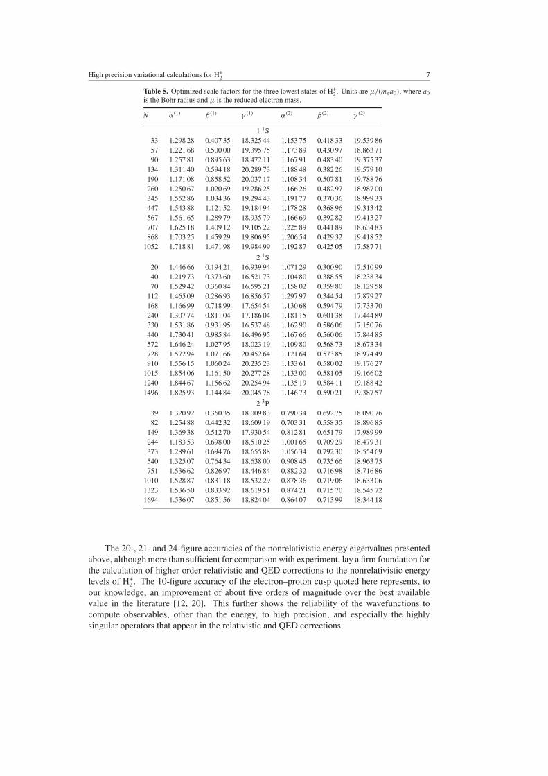
High precision variational calculations for H+2 7
Table 5. Optimized scale factors for the three lowest states of H+2 . Units are µ/(mea0), where a0
is the Bohr radius and µ is the reduced electron mass.
N α(1) β(1) γ (1) α(2) β(2) γ (2)
1 1S33 1.298 28 0.407 35 18.325 44 1.153 75 0.418 33 19.539 8657 1.221 68 0.500 00 19.395 75 1.173 89 0.430 97 18.863 7190 1.257 81 0.895 63 18.472 11 1.167 91 0.483 40 19.375 37
134 1.311 40 0.594 18 20.289 73 1.188 48 0.382 26 19.579 10190 1.171 08 0.858 52 20.037 17 1.108 34 0.507 81 19.788 76260 1.250 67 1.020 69 19.286 25 1.166 26 0.482 97 18.987 00345 1.552 86 1.034 36 19.294 43 1.191 77 0.370 36 18.999 33447 1.543 88 1.121 52 19.184 94 1.178 28 0.368 96 19.313 42567 1.561 65 1.289 79 18.935 79 1.166 69 0.392 82 19.413 27707 1.625 18 1.409 12 19.105 22 1.225 89 0.441 89 18.634 83868 1.703 25 1.459 29 19.806 95 1.206 54 0.429 32 19.418 52
1052 1.718 81 1.471 98 19.984 99 1.192 87 0.425 05 17.587 71
2 1S20 1.446 66 0.194 21 16.939 94 1.071 29 0.300 90 17.510 9940 1.219 73 0.373 60 16.521 73 1.104 80 0.388 55 18.238 3470 1.529 42 0.360 84 16.595 21 1.158 02 0.359 80 18.129 58
112 1.465 09 0.286 93 16.856 57 1.297 97 0.344 54 17.879 27168 1.166 99 0.718 99 17.654 54 1.130 68 0.594 79 17.733 70240 1.307 74 0.811 04 17.186 04 1.181 15 0.601 38 17.444 89330 1.531 86 0.931 95 16.537 48 1.162 90 0.586 06 17.150 76440 1.730 41 0.985 84 16.496 95 1.167 66 0.560 06 17.844 85572 1.646 24 1.027 95 18.023 19 1.109 80 0.568 73 18.673 34728 1.572 94 1.071 66 20.452 64 1.121 64 0.573 85 18.974 49910 1.556 15 1.060 24 20.235 23 1.133 61 0.580 02 19.176 27
1015 1.854 06 1.161 50 20.277 28 1.133 00 0.581 05 19.166 021240 1.844 67 1.156 62 20.254 94 1.135 19 0.584 11 19.188 421496 1.825 93 1.144 84 20.045 78 1.146 73 0.590 21 19.387 57
2 3P39 1.320 92 0.360 35 18.009 83 0.790 34 0.692 75 18.090 7682 1.254 88 0.442 32 18.609 19 0.703 31 0.558 35 18.896 85
149 1.369 38 0.512 70 17.930 54 0.812 81 0.651 79 17.989 99244 1.183 53 0.698 00 18.510 25 1.001 65 0.709 29 18.479 31373 1.289 61 0.694 76 18.655 88 1.056 34 0.792 30 18.554 69540 1.325 07 0.764 34 18.638 00 0.908 45 0.735 66 18.963 75751 1.536 62 0.826 97 18.446 84 0.882 32 0.716 98 18.716 86
1010 1.528 87 0.831 18 18.532 29 0.878 36 0.719 06 18.633 061323 1.536 50 0.833 92 18.619 51 0.874 21 0.715 70 18.545 721694 1.536 07 0.851 56 18.824 04 0.864 07 0.713 99 18.344 18
The 20-, 21- and 24-figure accuracies of the nonrelativistic energy eigenvalues presentedabove, although more than sufficient for comparison with experiment, lay a firm foundation forthe calculation of higher order relativistic and QED corrections to the nonrelativistic energylevels of H+
2. The 10-figure accuracy of the electron–proton cusp quoted here represents, toour knowledge, an improvement of about five orders of magnitude over the best availablevalue in the literature [12, 20]. This further shows the reliability of the wavefunctions tocompute observables, other than the energy, to high precision, and especially the highlysingular operators that appear in the relativistic and QED corrections.

8 M M Cassar and G W F Drake
References
[1] Jacobson P L, Fisher D S, Fehrenbach C W, Sturrus W G and Lundeen S R 1997 Phys. Rev. A 56 R4361Jacobson P L, Fisher D S, Fehrenbach C W, Sturrus W G and Lundeen S R 1998 Phys. Rev. A 57 4065 (erratum)
[2] Jacobson P L, Komara R A, Sturrus W G and Lundeen S R 2000 Phys. Rev. A 62 012509[3] Korobov V I 2001 Phys. Rev. A 63 044501[4] Sturrus W G, Hessels E A, Arcuni P W and Lundeen S R 1991 Phys. Rev. A 44 3032[5] Fu Z W, Hessels E A and Lundeen S R 1992 Phys. Rev. A 46 R5313[6] Nez F, Plimmer M D, Bourzeix S, Julien L, Biraben F, Felder R, Millerioux Y and de Natale P 1995 IEEE
Trans. Instrum. Meas. 44 568[7] Hilico L, Billy N, Gremaud B and Delande D 2001 J. Phys. B: At. Mol. Opt. Phys. 34 1[8] Hilico L private communication[9] Bailey D H and Frolov A M 2002 J. Phys. B: At. Mol. Opt. Phys. 35 4287
[10] Korobov V I 2000 Phys. Rev. A 61 064503[11] Yan Z-C, Zhang J-Y and Y L 2003 Phys. Rev. A 67 062504 See endnote 1[12] Frolov A M 2002 J. Phys. B: At. Mol. Opt. Phys. 35 L331[13] Cassar M M 1998 MSc Thesis University of Windsor[14] Drake G W F 1996 Atomic, Molecular and Optical Physics Handbook ed G W F Drake (Woodbury, NY: AIP)[15] Hilico L, Billy N, Gremaud B and Delande D 2000 Eur. Phys. J. D 12 449[16] Zare R N 1988 Angular Momentum: Understanding Spatial Aspects in Chemistry and Physics (Toronto: Wiley)[17] Drake G W F 1993 Long Range Casimir Forces: Theory and Recent Experiments in Atomic Systems
ed F S Levin and D A Micha (New York: Plenum)[18] Kono A and Hattori S 1985 Phys. Rev. A 31 1199[19] Bhatia A K 1998 Phys. Rev. A 58 2787[20] Bhatia A K and Drachman R J 1999 Phys. Rev. A 59 205
Bhatia A K and Drachman R J 1998 Phys. Rev. A 31 383[21] Cohen E R and Taylor B N 2000 Phys. Today 53 9[22] http://physics.nist.gov/cuu/Constants/index.html[23] Kato T 1957 Commun. Pure Appl. Math. 10 151[24] Pack R T and Brown W B 1966 J. Chem. Phys. 45 556[25] Drake G W F and Yan Zong-Chao 1994 Chem. Phys. Lett. 229 486[26] Moss R E 1999 J. Phys. B: At. Mol. Opt. Phys. 32 L89[27] Taylor J M, Yan Z-C, Dalgarno A and Babb J F 1999 Mol. Phys. 97 25

HIGH PRECISION SPECTROSCOPY
THEORY
– Hyperfine structure
– N.R. energies and relativistic corrections
– QED effects
Fine StructureIsotope Shift
⇒ internal check oftheory and experiment
4He – 6He
0
1s2p 3P
1
2
6 6
TransitionIsotope Shift⇒ nuclear radius
4He – 6He
0
1
2
1s2s 3S 1
6 6
Total TransitionFrequency⇒ QED shift
4He
0
1
2
1
6
Flow diagram for types of measurements.
transp08.tex, June/04