MITSUBISHI ELECTRIC RESEARCH LABORATORIEShttp://www.merl.com

Proportional-Integral Extremum Seeking for VaporCompression Systems

Burns, D.J.; Laughman, C.R.; Guay, M.

TR2019-032 June 22, 2019

AbstractIn this paper, we optimize vapor compression system power consumption through the appli-cation of a novel proportional–integral extremum seeking controller (PI-ESC) that convergesat the same timescale as the process. This extremum seeking method uses time-varying pa-rameter estimation to determine the local gradient in the map from manipulated inputs toperformance output. Additionally, the extremum seeking control law includes terms propor-tional to the estimated gradient, which requires subsequent modification of the estimationroutine in order to avoid bias. The PI-ESC algorithm is derived and compared to other meth-ods on a benchmark example that demonstrates the improved convergence rate of PI-ESC.PI-ESC is applied to the problem of compressor discharge temperature setpoint selectionfor a vapor compression system such that power consumption is driven to a minimum. Aphysicsbased simulation model of the vapor compression system is used to demonstrate thatwith PI-ESC, convergence to the optimal operating point occurs faster than the bandwidthof typical disturbances—enabling application of extremum seeking control to vapor compres-sion systems in environments under realistic operating conditions. Finally, experiments on aproduction room air conditioner installed in an adiabatic test facility validate the approachin the presence of significant noise and actuator and sensor quantization.

IEEE Transactions on Control Systems Technology

This work may not be copied or reproduced in whole or in part for any commercial purpose. Permission to copy inwhole or in part without payment of fee is granted for nonprofit educational and research purposes provided that allsuch whole or partial copies include the following: a notice that such copying is by permission of Mitsubishi ElectricResearch Laboratories, Inc.; an acknowledgment of the authors and individual contributions to the work; and allapplicable portions of the copyright notice. Copying, reproduction, or republishing for any other purpose shall requirea license with payment of fee to Mitsubishi Electric Research Laboratories, Inc. All rights reserved.

Copyright c© Mitsubishi Electric Research Laboratories, Inc., 2019201 Broadway, Cambridge, Massachusetts 02139

IEEE TRANSACTIONS ON CONTROL SYSTEMS TECHNOLOGY, VOL. XX, NO. YY, MONTH YYYY 1

Proportional–Integral Extremum Seekingfor Vapor Compression Systems

Daniel J. Burns,† Senior Member, IEEE, Christopher R. Laughman, Member, IEEEand Martin Guay, Senior Member, IEEE

Abstract—In this paper, we optimize vapor compression sys-tem power consumption through the application of a novelproportional–integral extremum seeking controller (PI-ESC) thatconverges at the same timescale as the process. This extremumseeking method uses time-varying parameter estimation to deter-mine the local gradient in the map from manipulated inputs toperformance output. Additionally, the extremum seeking controllaw includes terms proportional to the estimated gradient, whichrequires subsequent modification of the estimation routine inorder to avoid bias. The PI-ESC algorithm is derived andcompared to other methods on a benchmark example thatdemonstrates the improved convergence rate of PI-ESC.

PI-ESC is applied to the problem of compressor dischargetemperature setpoint selection for a vapor compression systemsuch that power consumption is driven to a minimum. A physics-based simulation model of the vapor compression system is usedto demonstrate that with PI-ESC, convergence to the optimaloperating point occurs faster than the bandwidth of typicaldisturbances—enabling application of extremum seeking controlto vapor compression systems in environments under realisticoperating conditions. Finally, experiments on a production roomair conditioner installed in an adiabatic test facility validate theapproach in the presence of significant noise and actuator andsensor quantization.

I. INTRODUCTION

VAPOR compression machines move thermal energy froma low temperature zone to a high temperature zone,

performing either cooling or heating depending on the config-uration of the refrigerant piping. The relative simplicity of themachine and its effective and robust performance has enabledthe vapor compression machine in various forms and packagesto become widely deployed, and it is critical to modern com-fort standards and the global food production and distributionindustries. It is the most common means for commercial andresidential space cooling [1], often employed for space orwater heating [2], and extensively used in refrigeration (bothstationary and mobile [3]), desalination [4], and cryogenicapplications [5].

In many control formulations for vapor compression ma-chines the evaporator superheat temperature is selected as aregulated variable for cycle efficiency and equipment protec-tion [6], [7], [8]. However, a measurement of the evaporatorsuperheat is often not available on production equipment.

D. J. Burns (burns@merl.com) and C. R. Laughman(laughman@merl.com) are with Mitsubishi Electric ResearchLaboratories, 201 Broadway, Cambridge, MA 02139.

M. Guay is with the Department of Chemical Engineering, Queen’s Univer-sity, Kingston, ON, Canada. email: martin.guay@chee.queensu.ca

† Corresponding author.

Instead, cycle efficiency can be maintained through the regu-lation of the compressor discharge temperature to a setpointthat depends on the heat load and the outdoor air temperaturedisturbances. The discharge temperature is often measuredfor equipment protection making it a commonly availablesignal, and because the refrigerant state at this location inthe cycle is always superheated, this signal is a one-to-onefunction of the disturbances over the full range of expectedoperating points [9]. Because discharge temperature changeswith heat loads and outdoor air temperatures, its setpointcannot be regulated to a constant, but instead must vary withexternal conditions. It is the aim of this paper to automate thegeneration of such setpoints.

However, determining these energy-optimal setpoints is notstraightforward. Models of the vapor compression system thatattempt to describe the influence of commanded inputs onthermodynamic behavior and power consumption are oftenlow in fidelity, and while they may have useful predictivecapabilities near the conditions at which they were calibrated,the environments into which these systems are deployed are sodiverse as to render comprehensive calibration and model tun-ing intractable. Therefore, relying on model-based strategiesfor realtime optimization is problematic.

Recently, model-free extremum seeking methods that op-erate in realtime and aim to optimize a cost have receivedincreased attention and have demonstrated improvements inthe optimization of vapor compression systems and otherHVAC applications [10], [11], [12], [13], [14]. To date, thedominant extremum seeking algorithm that appears in theHVAC research literature is the traditional perturbation-basedalgorithm first developed in the 1920s [15] and re-popularizedin the late 1990s by an elegant proof of convergence for ageneral class of nonlinear systems [16].

Most extremum seeking controllers can be viewed as agradient descent optimization algorithm implemented as afeedback controller [17] and therefore consists of two maincomponents: (1) an estimation part that determines the localgradient of the performance map with respect to the decisionvariables, and (2) a control law part that manipulates thedecision variables to steer the system to the optimizer of themap. In the traditional perturbation-based method, a sinusoidalterm is added to the input at a slower frequency than thenatural plant dynamics, inducing a sinusoidal response in theperformance metric and introducing a timescale slower thanthe process dynamics. The controller then filters this signal toobtain an estimate of the gradient. Averaging the perturbationintroduces yet another (and slower) time scale in the opti-

2 IEEE TRANSACTIONS ON CONTROL SYSTEMS TECHNOLOGY, VOL. XX, NO. YY, MONTH YYYY

mization process. Using a gradient estimate obtained in thisway, the control law integrates the estimated gradient to drivethe gradient to zero. As a result, the traditional perturbation-based extremum seeking converges to the neighborhood of theoptimum at about two timescales slower than the plant dy-namics due to inefficient estimation of the gradient, and slow(integral-action dominated) adaptation in the control law. Forthermal systems such as vapor compression machines wherethe dynamics are already on the order of tens of minutes, theslow convergence property of perturbation-based extremumseeking becomes an impediment to wide-scale deployment.

However, convergence rates can be improved by addressingboth components of the extremum seeking algorithm. Anefficient method for estimating gradients is developed thattreats the gradient as an unknown time-varying parameter tobe identified. Time-varying extremum seeking (TV-ESC) usesadaptive filtering techniques to estimate the parameters of thegradient—eliminating the timescale associated with averagingperturbations [18]. However, that method does not modify thecontrol law, and while convergence is significantly improvedcompared to the perturbation-based method, the control lawof TV-ESC remains integral-action dominated. In this paper,we apply PI-ESC [19] to vapor compression systems in whichthe algorithm estimates the gradient using the efficient time-varying approach, but also modifies the control law to includea term proportional to the value of the estimated gradient. Thisterm drives the system toward the optimum operating point atthe same timescale as the vapor compression system dynamics.

The remainder of this paper is organized as follows: Thevapor compression system and control objectives are describedin Section II. The discrete-time PI-ESC algorithm is thenderived in Section III and its convergence properties aredemonstrated in comparison to other ESC methods. Section IVpresents simulated and experimental results and concludingremarks are offered in Section V.

II. VAPOR COMPRESSION SYSTEM

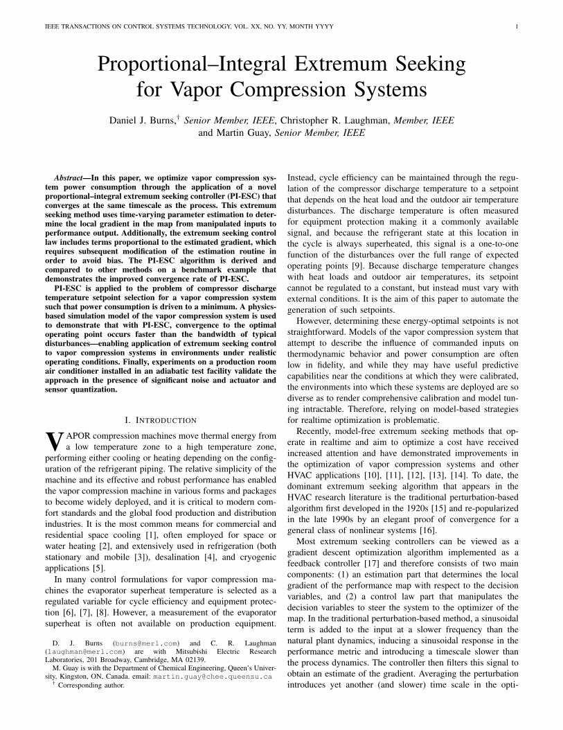
This section briefly describes the operation of the vaporcompression system (VCS) and control inputs, measurementsand objectives. The specific application considered in thispaper employs the VCS as an air conditioner, and thereforecertain assumptions on heat exchanger type, refrigerant flowdirection and control objectives have been made, althoughother applications of VCS (refrigeration, heat pumps, etc.) canbe considered with straightforward substitutions of machineconfigurations.

A. Physical Description

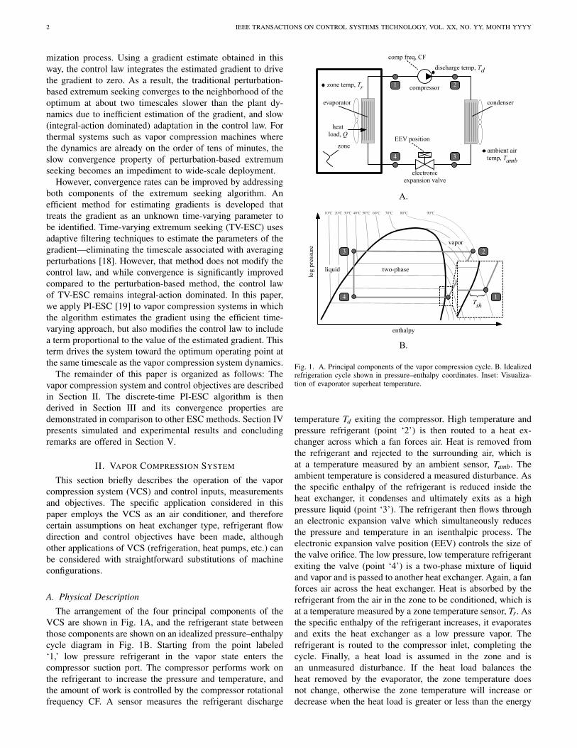
The arrangement of the four principal components of theVCS are shown in Fig. 1A, and the refrigerant state betweenthose components are shown on an idealized pressure–enthalpycycle diagram in Fig. 1B. Starting from the point labeled‘1,’ low pressure refrigerant in the vapor state enters thecompressor suction port. The compressor performs work onthe refrigerant to increase the pressure and temperature, andthe amount of work is controlled by the compressor rotationalfrequency CF. A sensor measures the refrigerant discharge

B.

compressor

electronic expansion valve

EEV position

comp freq, CF

A.

ambient air temp, Tamb

discharge temp, Td

zone

heat load, Q

zone temp, Tr 1

evaporator condenser

2

34

Tsh

23

4

enthalpy

log

pres

sure

liquid two-phase

vapor

10ºC 20ºC 30ºC 40ºC 50ºC 60ºC 70ºC 80ºC 90ºC

1

Fig. 1. A. Principal components of the vapor compression cycle. B. Idealizedrefrigeration cycle shown in pressure–enthalpy coordinates. Inset: Visualiza-tion of evaporator superheat temperature.

temperature Td exiting the compressor. High temperature andpressure refrigerant (point ‘2’) is then routed to a heat ex-changer across which a fan forces air. Heat is removed fromthe refrigerant and rejected to the surrounding air, which isat a temperature measured by an ambient sensor, Tamb. Theambient temperature is considered a measured disturbance. Asthe specific enthalpy of the refrigerant is reduced inside theheat exchanger, it condenses and ultimately exits as a highpressure liquid (point ‘3’). The refrigerant then flows throughan electronic expansion valve which simultaneously reducesthe pressure and temperature in an isenthalpic process. Theelectronic expansion valve position (EEV) controls the size ofthe valve orifice. The low pressure, low temperature refrigerantexiting the valve (point ‘4’) is a two-phase mixture of liquidand vapor and is passed to another heat exchanger. Again, a fanforces air across the heat exchanger. Heat is absorbed by therefrigerant from the air in the zone to be conditioned, which isat a temperature measured by a zone temperature sensor, Tr. Asthe specific enthalpy of the refrigerant increases, it evaporatesand exits the heat exchanger as a low pressure vapor. Therefrigerant is routed to the compressor inlet, completing thecycle. Finally, a heat load is assumed in the zone and isan unmeasured disturbance. If the heat load balances theheat removed by the evaporator, the zone temperature doesnot change, otherwise the zone temperature will increase ordecrease when the heat load is greater or less than the energy

BURNS et al.: PI-ESC FOR VAPOR COMPRESSION SYSTEMS 3

removed by the evaporator.Remark 1: Note the lines of constant temperature in Fig. 1B.

The evaporating and condensing processes of refrigerant phasechange occurs at a constant temperature (within the ‘two-phase’ region between the saturation curves of Fig. 1B) whenthe refrigerant used is a pure or near-azeotropic fluid [20], as isthe case for many commercially-available systems. Therefore,the thermodynamic state of refrigerant undergoing a phasechange process is not measurable from temperature or pressuresensors.

B. Evaporator Superheat vs. Discharge Temperature

Consider again the refrigerant in the evaporator. As heatis absorbed, the state changes from a mostly liquid two-phase mixture to a mostly vapor mixture, ultimately reaching asaturated vapor state during an isothermal process. As furtherheat is absorbed by a saturated vapor, a measurable changein temperature occurs. This increase in temperature above thesaturation temperature is called the superheat temperature Tsh,

Tsh = T1−Tsat, p1 , (1)

where T1 is the temperature of the refrigerant at point ’1’on Fig. 1B, and Tsat, p1 is the saturation temperature of therefrigerant at that pressure p1. Note that superheat temperatureis not defined for values less than zero (see Remark above.)

Many control designs use Tsh as a process variable andregulate it to a small positive value using the EEV. A lowsuperheat temperature ensures that the majority of the evapo-rator contains two-phase refrigerant, which has a much higherheat transfer coefficient than refrigerant in the vapor state,and therefore low Tsh is associated with good cycle efficiency.However, disturbances can perturb the superheat temperatureto zero, causing the feedback loop to open. As a result, manyTsh controllers have low gain in order to tolerate occasionalopen loop operation, and this leads to the well-known issue ofvalve ‘hunting,’ which is limit cycling induced by low gainfeedback [21], whether that feedback is mechanical as forthermostatic expansion valves or electronic as for EEVs. Incontrast to previous work, we select the compressor dischargetemperature Td as a process variable. As seen from point ‘2’of Fig. 1B, the refrigerant at the compressor outlet is far fromthe saturation boundary and within the measurable superheatedregion where temperatures at this point in the cycle are a one-to-one function of the disturbances, which maintains systemobservability and enables higher gain feedback.

However, while controlling Td has certain advantages, itcannot be regulated to a constant, but instead must be sched-uled on system disturbances. In following sections, we useextremum seeking to determine setpoints for a Td regulator.

C. Controller Architecture

The control objective is to regulate the zone temperature Trto a setpoint determined by an occupant, rejecting heat load Qand ambient air temperature Tamb disturbances. Further, powerconsumption P must be minimized at steady state. The systemactuators are the compressor frequency CF, and electronicexpansion valve position EEV. We assume that the fan speeds

VCS & Zone

Tamb, Q

Tr Setpt

ESC

P

Optimization Target

ykuk

K2

K1 Tr

Td

CF

EEV

-

-

Td SetptK

Power

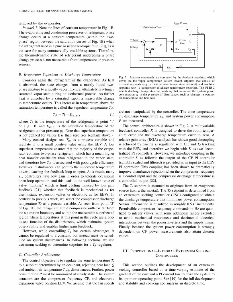
Fig. 2. Actuator commands are computed by the feedback regulator, whichdrives the the vapor compression system toward setpoints that consist ofexternal setpoints (e.g., a desired zone temperature setpoint) and machinesetpoints (e.g., a compressor discharge temperature setpoint). The PI-ESCselects discharge temperature setpoints uk that minimize the system powerconsumption yk in the presence of disturbances such as changes in outdoorair temperature and heat load.

are not manipulated by the controller. The zone temperatureTr, discharge temperature Td , and system power consumptionP are measured.

The control architecture is shown in Fig. 2. A multivariablefeedback controller K is designed to drive the room temper-ature error and the discharge temperature error to zero. Arelative gain array (RGA) analysis has shown good decouplingis achieved by pairing Tr regulation with CF, and Td trackingwith the EEV, and therefore we begin with K as two decen-tralized PI controllers. However, we introduce coupling in thecontroller K as follows: the output of the CF PI controller(suitably scaled and filtered) is provided as an input to the EEVPI controller. This coupling has been shown to dramaticallyimprove disturbance rejection when the compressor frequencyis a control input and the compressor discharge temperature isa controlled output [22].

The Tr setpoint is assumed to originate from an exogenoussource (i.e., a thermostat). The Td setpoint is determined froman extremum seeking controller (ESC) configured to obtainthe discharge temperature that minimizes power consumption.Sensor information is quantized in roughly 0.5 C increments.Permissible compressor frequency commands in Hz are quan-tized to integer values, with some additional ranges excludedto avoid mechanical resonances and detrimental electricalinteractions between the power inverters and the supply mains.Finally, because the system power consumption is stronglydependent on CF, power measurements also attain discretevalues.

III. PROPORTIONAL–INTEGRAL EXTREMUM SEEKINGCONTROLLER

This section outlines the development of an extremumseeking controller based on a time-varying estimate of thegradient of the cost and a PI control law to drive the system toits optimum operating point. See [19] for the full developmentand stability and convergence analysis in discrete time.

4 IEEE TRANSACTIONS ON CONTROL SYSTEMS TECHNOLOGY, VOL. XX, NO. YY, MONTH YYYY

Parameter Estimator Control Law

yk ✓kMk

ek

⌃�1kRk

Mk =1↵⌃

�1k wk

1 + 1↵wT

k ⌃�1k wk

Rk =1↵2⌃

�1k wT

k wk⌃�1k

1 + 1↵wT

k ⌃�1k wk

<latexit sha1_base64="d/3HuynIj4CKb2WQqGUtvAwTKrg=">AAACtHiclVFNT+MwEHXCV+myUODIxaJaaSW0KEYIuCAhuHBBKh+lSE0JE9dprThOZDugKsov5MaNf4PT9gAtHHYk209v3szYz2EmuDae9+64C4tLyyu11fqvtd/rG43NrXud5oqyNk1Fqh5C0ExwydqGG8EeMsUgCQXrhPFFle88M6V5Ku/MKGO9BAaSR5yCsVTQeL0KYnyK/UgBLSY7KQsfRDaE0r/lgwSC+LH4R8qXIC4LsjereanSd/NS7Pt1fPNz88eDuZqqjz2+0P8zMmg0vX1vHHgekCloomm0gsab309pnjBpqACtu8TLTK8AZTgVrKz7uWYZ0BgGrGuhhITpXjE2vcR/LNPHUarskgaP2c8VBSRaj5LQKhMwQz2bq8jvct3cRCe9gsssN0zSyaAoF9ikuPpB3OeKUSNGFgBV3N4V0yFYi4z957o1gcw+eR7cH+wTi68Pm2fnUztqaAftor+IoGN0hi5RC7URdYjTcZ4ccI9c36Uum0hdZ1qzjb6EKz8A8uPYkQ==</latexit><latexit sha1_base64="d/3HuynIj4CKb2WQqGUtvAwTKrg=">AAACtHiclVFNT+MwEHXCV+myUODIxaJaaSW0KEYIuCAhuHBBKh+lSE0JE9dprThOZDugKsov5MaNf4PT9gAtHHYk209v3szYz2EmuDae9+64C4tLyyu11fqvtd/rG43NrXud5oqyNk1Fqh5C0ExwydqGG8EeMsUgCQXrhPFFle88M6V5Ku/MKGO9BAaSR5yCsVTQeL0KYnyK/UgBLSY7KQsfRDaE0r/lgwSC+LH4R8qXIC4LsjereanSd/NS7Pt1fPNz88eDuZqqjz2+0P8zMmg0vX1vHHgekCloomm0gsab309pnjBpqACtu8TLTK8AZTgVrKz7uWYZ0BgGrGuhhITpXjE2vcR/LNPHUarskgaP2c8VBSRaj5LQKhMwQz2bq8jvct3cRCe9gsssN0zSyaAoF9ikuPpB3OeKUSNGFgBV3N4V0yFYi4z957o1gcw+eR7cH+wTi68Pm2fnUztqaAftor+IoGN0hi5RC7URdYjTcZ4ccI9c36Uum0hdZ1qzjb6EKz8A8uPYkQ==</latexit><latexit sha1_base64="d/3HuynIj4CKb2WQqGUtvAwTKrg=">AAACtHiclVFNT+MwEHXCV+myUODIxaJaaSW0KEYIuCAhuHBBKh+lSE0JE9dprThOZDugKsov5MaNf4PT9gAtHHYk209v3szYz2EmuDae9+64C4tLyyu11fqvtd/rG43NrXud5oqyNk1Fqh5C0ExwydqGG8EeMsUgCQXrhPFFle88M6V5Ku/MKGO9BAaSR5yCsVTQeL0KYnyK/UgBLSY7KQsfRDaE0r/lgwSC+LH4R8qXIC4LsjereanSd/NS7Pt1fPNz88eDuZqqjz2+0P8zMmg0vX1vHHgekCloomm0gsab309pnjBpqACtu8TLTK8AZTgVrKz7uWYZ0BgGrGuhhITpXjE2vcR/LNPHUarskgaP2c8VBSRaj5LQKhMwQz2bq8jvct3cRCe9gsssN0zSyaAoF9ikuPpB3OeKUSNGFgBV3N4V0yFYi4z957o1gcw+eR7cH+wTi68Pm2fnUztqaAftor+IoGN0hi5RC7URdYjTcZ4ccI9c36Uum0hdZ1qzjb6EKz8A8uPYkQ==</latexit><latexit sha1_base64="d/3HuynIj4CKb2WQqGUtvAwTKrg=">AAACtHiclVFNT+MwEHXCV+myUODIxaJaaSW0KEYIuCAhuHBBKh+lSE0JE9dprThOZDugKsov5MaNf4PT9gAtHHYk209v3szYz2EmuDae9+64C4tLyyu11fqvtd/rG43NrXud5oqyNk1Fqh5C0ExwydqGG8EeMsUgCQXrhPFFle88M6V5Ku/MKGO9BAaSR5yCsVTQeL0KYnyK/UgBLSY7KQsfRDaE0r/lgwSC+LH4R8qXIC4LsjereanSd/NS7Pt1fPNz88eDuZqqjz2+0P8zMmg0vX1vHHgekCloomm0gsab309pnjBpqACtu8TLTK8AZTgVrKz7uWYZ0BgGrGuhhITpXjE2vcR/LNPHUarskgaP2c8VBSRaj5LQKhMwQz2bq8jvct3cRCe9gsssN0zSyaAoF9ikuPpB3OeKUSNGFgBV3N4V0yFYi4z957o1gcw+eR7cH+wTi68Pm2fnUztqaAftor+IoGN0hi5RC7URdYjTcZ4ccI9c36Uum0hdZ1qzjb6EKz8A8uPYkQ==</latexit>

yk = yk�1 + Kek�1 + �Tk�1✓k�1 + wT

k�1(✓k � ✓k�1)<latexit sha1_base64="O0YEj5JXDJX5AkKxOherVjCPof4=">AAACZHicbZFLS8NAFIUn8VGtr6i4EmSwCIpYEinoRhDcCG4U2io0tUymt2bI5MHMjVJC/6Q7l278HU5rW7T1wsDHOecyyZkgk0Kj635Y9sLi0nJpZbW8tr6xueVs7zR1misODZ7KVD0FTIMUCTRQoISnTAGLAwmPQXQz9B9fQWmRJnXsZ9CO2UsieoIzNFLHKfyQYdEfdCJ6RSdcRGfegJ7SO5iin4XiuahPvFHSxxCQTeNvv/zjP4GInv2zcdJxKm7VHQ2dB28MFTKe+47z7ndTnseQIJdM65bnZtgumELBJQzKfq4hYzxiL9AymLAYdLsYlTSgR0bp0l6qzEmQjtTfGwWLte7HgUnGDEM96w3F/7xWjr3LdiGSLEdI+M9FvVxSTOmwcdoVCjjKvgHGlTDfSnnIFONo3qVsSvBmf3kemudVz/BDrXJdG9exQvbJITkmHrkg1+SW3JMG4eTTKlmOtW192ev2rr33E7Wt8c4u+TP2wTf3dbaX</latexit><latexit sha1_base64="O0YEj5JXDJX5AkKxOherVjCPof4=">AAACZHicbZFLS8NAFIUn8VGtr6i4EmSwCIpYEinoRhDcCG4U2io0tUymt2bI5MHMjVJC/6Q7l278HU5rW7T1wsDHOecyyZkgk0Kj635Y9sLi0nJpZbW8tr6xueVs7zR1misODZ7KVD0FTIMUCTRQoISnTAGLAwmPQXQz9B9fQWmRJnXsZ9CO2UsieoIzNFLHKfyQYdEfdCJ6RSdcRGfegJ7SO5iin4XiuahPvFHSxxCQTeNvv/zjP4GInv2zcdJxKm7VHQ2dB28MFTKe+47z7ndTnseQIJdM65bnZtgumELBJQzKfq4hYzxiL9AymLAYdLsYlTSgR0bp0l6qzEmQjtTfGwWLte7HgUnGDEM96w3F/7xWjr3LdiGSLEdI+M9FvVxSTOmwcdoVCjjKvgHGlTDfSnnIFONo3qVsSvBmf3kemudVz/BDrXJdG9exQvbJITkmHrkg1+SW3JMG4eTTKlmOtW192ev2rr33E7Wt8c4u+TP2wTf3dbaX</latexit><latexit sha1_base64="O0YEj5JXDJX5AkKxOherVjCPof4=">AAACZHicbZFLS8NAFIUn8VGtr6i4EmSwCIpYEinoRhDcCG4U2io0tUymt2bI5MHMjVJC/6Q7l278HU5rW7T1wsDHOecyyZkgk0Kj635Y9sLi0nJpZbW8tr6xueVs7zR1misODZ7KVD0FTIMUCTRQoISnTAGLAwmPQXQz9B9fQWmRJnXsZ9CO2UsieoIzNFLHKfyQYdEfdCJ6RSdcRGfegJ7SO5iin4XiuahPvFHSxxCQTeNvv/zjP4GInv2zcdJxKm7VHQ2dB28MFTKe+47z7ndTnseQIJdM65bnZtgumELBJQzKfq4hYzxiL9AymLAYdLsYlTSgR0bp0l6qzEmQjtTfGwWLte7HgUnGDEM96w3F/7xWjr3LdiGSLEdI+M9FvVxSTOmwcdoVCjjKvgHGlTDfSnnIFONo3qVsSvBmf3kemudVz/BDrXJdG9exQvbJITkmHrkg1+SW3JMG4eTTKlmOtW192ev2rr33E7Wt8c4u+TP2wTf3dbaX</latexit><latexit sha1_base64="O0YEj5JXDJX5AkKxOherVjCPof4=">AAACZHicbZFLS8NAFIUn8VGtr6i4EmSwCIpYEinoRhDcCG4U2io0tUymt2bI5MHMjVJC/6Q7l278HU5rW7T1wsDHOecyyZkgk0Kj635Y9sLi0nJpZbW8tr6xueVs7zR1misODZ7KVD0FTIMUCTRQoISnTAGLAwmPQXQz9B9fQWmRJnXsZ9CO2UsieoIzNFLHKfyQYdEfdCJ6RSdcRGfegJ7SO5iin4XiuahPvFHSxxCQTeNvv/zjP4GInv2zcdJxKm7VHQ2dB28MFTKe+47z7ndTnseQIJdM65bnZtgumELBJQzKfq4hYzxiL9AymLAYdLsYlTSgR0bp0l6qzEmQjtTfGwWLte7HgUnGDEM96w3F/7xWjr3LdiGSLEdI+M9FvVxSTOmwcdoVCjjKvgHGlTDfSnnIFONo3qVsSvBmf3kemudVz/BDrXJdG9exQvbJITkmHrkg1+SW3JMG4eTTKlmOtW192ev2rr33E7Wt8c4u+TP2wTf3dbaX</latexit>

predict output:

correct parameterestimate:

update covariance:

uk uk✓1,k z�1

1 � z�1

�1

⌧I

�kg

-

uk � uk pre-condition

yk

-predict output

z�1

1 � 1↵z�1

z�1

1 � z�1

pre-condition: �k = [1, (uk � uk)T ]T

0 00 I

�

!k

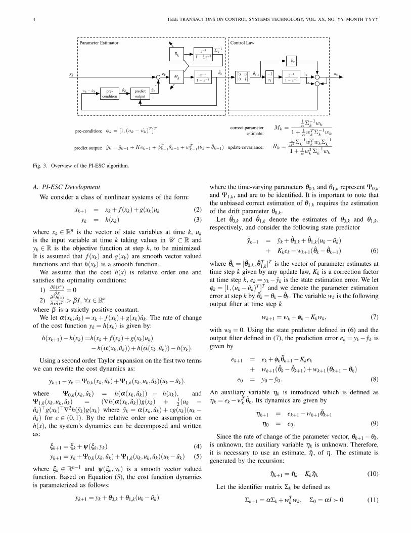
Fig. 3. Overview of the PI-ESC algorithm.

A. PI-ESC Development

We consider a class of nonlinear systems of the form:

xk+1 = xk + f (xk)+g(xk)uk (2)yk = h(xk) (3)

where xk ∈ Rn is the vector of state variables at time k, ukis the input variable at time k taking values in U ⊂ R andyk ∈ R is the objective function at step k, to be minimized.It is assumed that f (xk) and g(xk) are smooth vector valuedfunctions and that h(xk) is a smooth function.

We assume that the cost h(x) is relative order one andsatisfies the optimality conditions:

1) ∂h(x∗)∂x = 0

2) ∂ 2h(x)∂x∂xT > β I, ∀x ∈ Rn

where β is a strictly positive constant.We let α(xk, uk) = xk + f (xk)+g(xk)uk. The rate of change

of the cost function yk = h(xk) is given by:

h(xk+1)−h(xk) =h(xk + f (xk)+g(xk)uk)

−h(α(xk, uk))+h(α(xk, uk))−h(xk).

Using a second order Taylor expansion on the first two termswe can rewrite the cost dynamics as:

yk+1− yk = Ψ0,k(xk, uk)+Ψ1,k(xk,uk, uk)(uk− uk).

where Ψ0,k(xk, uk) = h(α(xk, uk)) − h(xk), andΨ1,k(xk,uk, uk) = (∇h(α(xk, uk))g(xk) + 1

2 (uk −uk)>g(xk)

>∇2h(yk)g(xk) where yk = α(xk, uk) + cg(xk)(uk −uk) for c ∈ (0,1). By the relative order one assumption onh(x), the system’s dynamics can be decomposed and writtenas:

ξk+1 = ξk +ψ(ξk,yk) (4)yk+1 = yk +Ψ0,k(xk, uk)+Ψ1,k(xk,uk, uk)(uk− uk) (5)

where ξk ∈ Rn−1 and ψ(ξk, yk) is a smooth vector valuedfunction. Based on Equation (5), the cost function dynamicsis parameterized as follows:

yk+1 = yk +θ0,k +θ1,k(uk− uk)

where the time-varying parameters θ0,k and θ1,k represent Ψ0,kand Ψ1,k, and are to be identified. It is important to note thatthe unbiased correct estimation of θ1,k requires the estimationof the drift parameter θ0,k.

Let θ0,k and θ1,k denote the estimates of θ0,k and θ1,k,respectively, and consider the following state predictor

yk+1 = yk + θ0,k + θ1,k(uk− uk)

+ Kkek−wk+1(θk− θk+1) (6)

where θk = [θ0,k, θT1,k]

T is the vector of parameter estimates attime step k given by any update law, Kk is a correction factorat time step k, ek = yk− yk is the state estimation error. We letφk = [1,(uk− uk)

T ]T and we denote the parameter estimationerror at step k by θk = θk− θk. The variable wk is the followingoutput filter at time step k

wk+1 = wk +φk−Kkwk, (7)

with w0 = 0. Using the state predictor defined in (6) and theoutput filter defined in (7), the prediction error ek = yk− yk isgiven by

ek+1 = ek +φkθk+1−Kkek

+ wk+1(θk− θk+1)+wk+1(θk+1−θk)

e0 = y0− y0. (8)

An auxiliary variable ηk is introduced which is defined asηk = ek−wT

k θk. Its dynamics are given by

ηk+1 = ek+1−wk+1θk+1

η0 = e0. (9)

Since the rate of change of the parameter vector, θk+1−θk,is unknown, the auxiliary variable ηk is unknown. Therefore,it is necessary to use an estimate, η , of η . The estimate isgenerated by the recursion:

ηk+1 = ηk−Kkηk (10)

Let the identifier matrix Σk be defined as

Σk+1 = αΣk +wTk wk, Σ0 = αI � 0 (11)

BURNS et al.: PI-ESC FOR VAPOR COMPRESSION SYSTEMS 5

with an inverse generated by the recursion

Σ−1k+1 =Σ

−1k +

(1α−1

)Σ−1k

− 1α2 Σ

−1k wk(1+

1α

wTk Σ−1k wk)

−1wTk Σ−1k (12)

Using (6), (7), and (10), the parameter update law is

θk+1 = θk +1α

Σ−1k wT

k

(I +

1α

wkΣ−1k wT

k

)−1

(ek− ηk) (13)

In order to prevent any peaking arising from the estimation, theparameter estimate are constrained to remain inside compactconvex set in the parameter space denoted by Θ. Consequently,the true value, θk, is assumed to be contained inside Θ.To ensure that the parameter estimates remain within theconstraint set Θ, we use a projection operator [18], [23]

¯θk+1 = Proj{θk+Σ

−1k wT

k(I +wkΣ

−1k wT

k)−1

(ek− ηk),Θ} (14)

which completes the parameter estimation component of thecontroller.

Finally, the proposed control law is given by:

uk =−kgθ1,k + uk (15)

uk+1 = uk−1τI

θ1,k. (16)

where kg and τI are positive constants to be assigned.

B. PI-ESC Summary

The final PI-ESC algorithm consists of a time varyingparameter estimation routine for determining θ0,k and θ1,kand consists of Equations (6), (7), (10), (12), and (14) withtuning parameters K and α . The control law is given byEquations (15) and (16) and contains terms proportional tothe estimated gradient and with integral action necessary toidentify optimal equilibrium conditions, and is tuned using theparameters kg and τI . A block diagram of the PI-ESC algo-rithm summarizing the main signal flow is shown in Figure 3.Guidance for tuning the parameters of these equations can befound in [19].

Note that the PI-ESC algorithm does not require averagingthe effect of the perturbation as with traditional perturbation-based extremum seeking. For this reason, proportional-integralextremum seeking converges substantially faster, as demon-strated in the following comparison.

C. Comparison of extremum seeking methods

This section discusses the convergence performance ofthree extremum seeking controllers applied to a previouslypublished example problem [9]. Traditional perturbation-basedextremum seeking control [24], time-varying extremum seek-ing control [18] and proportional–integral extremum seekingcontrol [19] are each applied to the problem of finding inputvalues to a simple Hammerstein system that minimize its

0 100 200 300 400 500 600 700 800 900 10000

1

2

3

0 100 200 300 400 500 600 700 800 900 1000

0

20

40

60

ESC

Optimization Target

A.

B.

uk yk

xk+1 = 0.8xk + uk

yz = (xk � 3)2 + 1

Perturbation ESCTime-varying ESCProportional-Integral ESCPerfect control (with prior knowledge)uk

yk

Timestep, k

80 100 120 140 160 180 200 220 2400

1

2

3

80 100 120 140 160 180 200 220 240

0

20

40

60

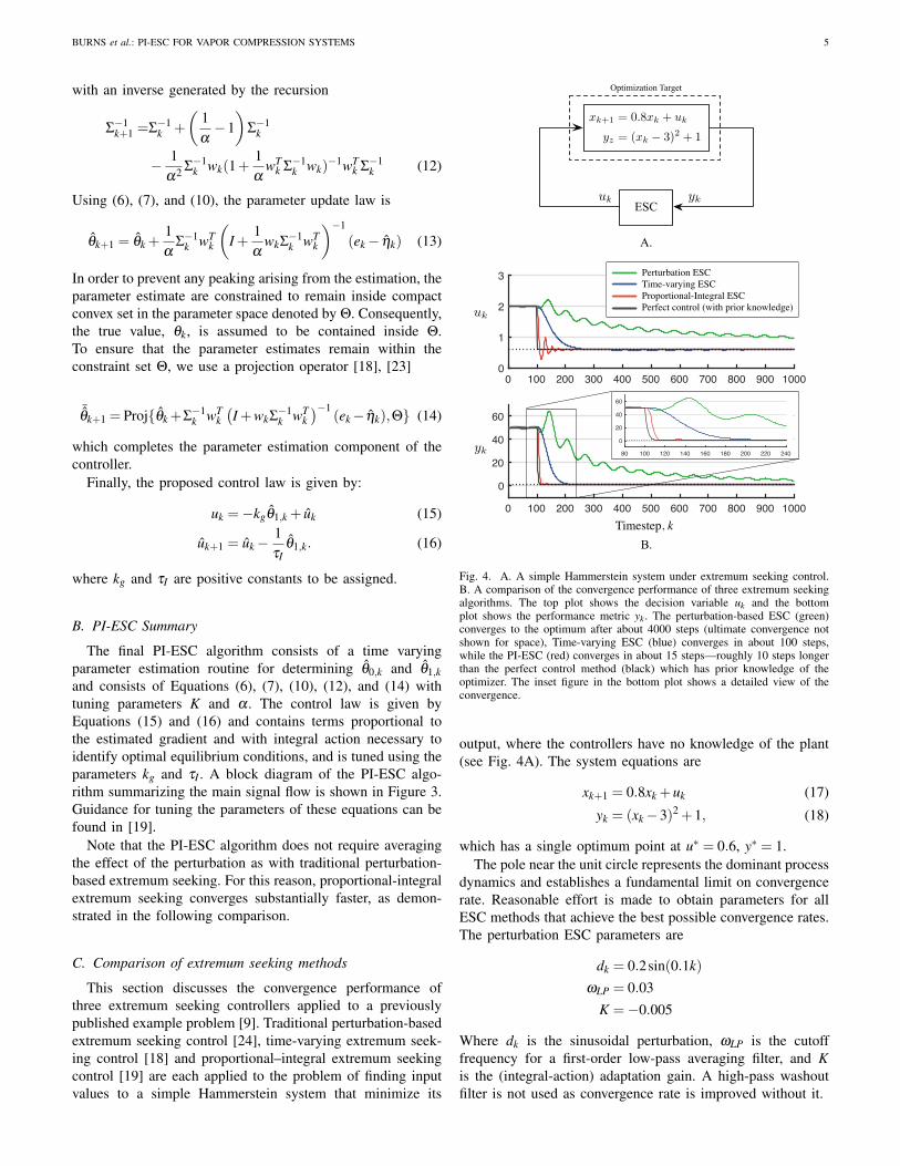
Fig. 4. A. A simple Hammerstein system under extremum seeking control.B. A comparison of the convergence performance of three extremum seekingalgorithms. The top plot shows the decision variable uk and the bottomplot shows the performance metric yk . The perturbation-based ESC (green)converges to the optimum after about 4000 steps (ultimate convergence notshown for space), Time-varying ESC (blue) converges in about 100 steps,while the PI-ESC (red) converges in about 15 steps—roughly 10 steps longerthan the perfect control method (black) which has prior knowledge of theoptimizer. The inset figure in the bottom plot shows a detailed view of theconvergence.

output, where the controllers have no knowledge of the plant(see Fig. 4A). The system equations are

xk+1 = 0.8xk +uk (17)

yk = (xk−3)2 +1, (18)

which has a single optimum point at u∗ = 0.6, y∗ = 1.The pole near the unit circle represents the dominant process

dynamics and establishes a fundamental limit on convergencerate. Reasonable effort is made to obtain parameters for allESC methods that achieve the best possible convergence rates.The perturbation ESC parameters are

dk = 0.2sin(0.1k)

ωLP = 0.03K =−0.005

Where dk is the sinusoidal perturbation, ωLP is the cutofffrequency for a first-order low-pass averaging filter, and Kis the (integral-action) adaptation gain. A high-pass washoutfilter is not used as convergence rate is improved without it.

6 IEEE TRANSACTIONS ON CONTROL SYSTEMS TECHNOLOGY, VOL. XX, NO. YY, MONTH YYYY

The parameters used for the TV-ESC are

dk = 0.001sin(0.1k) ki = 0.001α = 0.1 ε = 0.4,

where ki is the (integral-action) adaptation gain, α is theestimator forgetting factor, and ε is the estimator timescaleseparation parameter.

The parameters used for the PI-ESC are

dk = 0.001sin(0.2k), τI = 60α = 0.5, kg = 0.0003

Kk = 0.1,

where τI is the integral time constant, kg is the proportionalgain and is computed from the relationship kg = 1/(τ2

I ), α isthe estimator forgetting factor, and Kk is the estimation gain.See [18] for detailed parameter definitions.

Simulations are performed starting from an initial inputvalue of u0 = 2 and the ESC methods are turned on after100 steps. The resulting simulations are shown in Fig. 4B.The perturbation ESC method converges to a neighborhoodaround the optimum in about 4000 steps (not shown in thefigure), the TV-ESC method converges in about 100 steps,while the PI-ESC method converges in about 15 steps. Theresulting controller performance is compared to the responseobtained from a controller that has a priori knowledge of thesystem optimizer and applied directly in one time step, forwhich the output settles in about 10 steps. Thus, the PI-ESCapproach convergence to the optimizer at the same timescaleas the process.

IV. RESULTS

The fast convergence characteristic of PI-ESC is well suitedto the optimization of thermal systems with their associatedlong time constants. In this section, we apply the PI-ESCalgorithm to the problem of selecting setpoints for the dis-charge temperature of a vapor compression system. In the firstpart, a multiphysics-based model of the vapor compressionsystem is detailed and used to compare TV-ESC and PI-ESCfor an initial condition response and disturbance rejectionresponse wherein the boundary conditions are changed. Inthe second part, experimental work is presented demonstratingconvergence on a production-grade room air conditioner.

A. Model Description

A detailed model1 describing the nonlinear dynamics ofthe vapor compression cycle is developed using the equation-oriented modeling language Modelica [25]. Physics-basedmodels are constructed for the four principal componentsshown in Fig. 1A: the evaporating and condensing heatexchangers, the compressor, and the electronic expansionvalve. Algebraic models are used for the compressor and the

1We emphasize here that although a brief discussion is offered on modeldevelopment, the ESC algorithms themselves are not model-based. Themodel in this section is used as a synthetic plant for controller evaluationand comparison, and does not inform PI-ESC design beyond satisfying theassumptions in Section III-A.

45 50 55 60 65 70 75 80 85

520

560

600

640

680

720

760

Pow

er (W

)

Td Setpt (C)

Time-varying ESCProportional-Integral ESCSteady-state maps

Start

Map Tamb = 35ºC

Map Tamb = 40ºC

End (init cond resp)

End(dist reject)

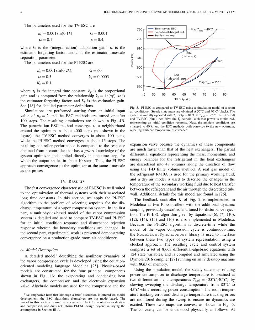
Fig. 5. PI-ESC is compared to TV-ESC using a simulation model of a roomair conditioner. Steady state maps are obtained at 35◦C and 40◦C (black). Thesystem is initially operated with Td Setpt= 81◦C at Tamb = 35◦C. PI-ESC (red)and TV-ESC (blue) then drive the Td setpoint such that power is minimized,representing an initial condition response. Next, the ambient conditions arechanged to 40◦C and the ESC methods both converge to the new optimum,rejecting ambient temperature disturbance.

expansion valve because the dynamics of these componentsare much faster than that of the heat exchangers. The partialdifferential equations representing the mass, momentum, andenergy balances for the refrigerant in the heat exchangersare discretized into 48 volumes along the direction of flowusing the 1-D finite volume method. A real gas model ofthe refrigerant R410A is used for the primary working fluid,and a dry air model is used to describe the changes in thetemperature of the secondary working fluid due to heat transferbetween the refrigerant and the air through the discretized tubewall. Additional details for this model are found in [26].

The feedback controller K of Fig. 2 is implemented inModelica as two PI controllers with the additional dynamiccoupling previously described and tuned for disturbance rejec-tion. The PI-ESC algorithm given by Equations (6), (7), (10),(12), (14), (15) and (16) is also implemented in Modelica.Because the PI-ESC algorithm is discrete-time while themodel of the vapor compression cycle is continuous-time,the Modelica.Synchronous library is used to interfacebetween these two types of system representation using aclocked approach. The resulting cycle and control systemcomprise a set of 8,663 differential-algebraic equations with124 state variables, and is compiled and simulated using theDymola 2016 compiler [27] running on an i7 desktop machinewith 8GB of memory.

Using the simulation model, the steady-state map relatingpower consumption to discharge temperature is obtained attwo different ambient temperatures Tamb = {35◦C,40◦C} byslowing sweeping the discharge temperature from 83◦C to45◦C while recording power consumption. The room temper-ature tracking error and discharge temperature tracking errorsare monitored during the sweep to ensure no dynamics areexcited. These two maps are convex, as shown in Fig. 5.The convexity can be understood physically as follows: At

BURNS et al.: PI-ESC FOR VAPOR COMPRESSION SYSTEMS 7

the high temperature end of this sweep, the elevated dischargetemperatures require relatively little refrigerant returning tothe compressor and therefore the compressor discharge tem-perature feedback loop selects expansion valve commandsthat are more closed than optimal. As a result, the amountof refrigerant entering the evaporator is restricted, causing ahigh degree of superheating. As the compressor temperaturesetpoint is reduced, the feedback loop opens the expansionvalve, allowing more refrigerant into the evaporator, which inturn provides more cooling to the zone. As the zone coolsbelow the setpoint temperature, the compressor frequency isreduced by the zone temperature feedback controller, therebyreducing power consumption. This explains the downwardslopes in the steady state maps from about 83◦C toward thetwo optimizers.

As the downward ramp continues through the optimum andtoward lower Td setpoints, the power consumption increases.This is explained by the reduction in the system pressure ratioand corresponding loss of cooling capacity caused by openingthe expansion valve too much. When the compressor dischargetemperature setpoint is set to a value lower than optimum, theexpansion valve is opened, causing the evaporating pressureto increase and the condensing pressure to decrease. In orderto compensate for the reduced cooling capacity, the zone tem-perature feedback loop increases the compressor frequency,which in turn increases power consumption at setpoint valueslower than the respective map minimizers.

B. Simulation results

Simulations are performed comparing TV-ESC to PI-ESCusing the model. We initially tried perturbation ESC, butconvergence time was similar in scale to the Hammersteinsystem of Fig. 4 and too long to be practical. Two types ofsystem responses are tested: the ESC algorithms are initializedat a suboptimal operating point and converge to the optimizerunder fixed conditions, demonstrating the initial conditionresponse, and a subsequent step change in ambient temperaturedemonstrates disturbance rejection performance.

In the following simulations, TV-ESC and PI-ESC methodsare executed every 60 seconds. The parameters used for theTV-ESC are

dk = 0.5sin(0.2k) ki = 0.02α = 0.05 ε = 0.9,

and the parameters used for the PI-ESC are

dk = 0.5sin(0.3k), τI = 1α = 0.06, kg = 0.5

Kk = 0.4, Θk = 50.

Initial values for the PI-ESC parameters are obtained us-ing the guidance offered in [19]. We have found it helpfulto further refine these parameters in a iterative manner bysimulating an approximate model of the optimization target.In this approach, we assume the vapor compression systemis a Hammerstein system of the form (17)-(18), with suitablesubstitutions for a the dominant pole and approximate convex

0 120 240 360 480 600 720 840 960 1080455055606570758085

0 120 240 360 480 600 720 840 960 1080

520560600640680720760

0 120 240 360 480 600 720 840 960 108025

26

27

28

29

30

Time-varying ESCProportional-Integral ESC

Time (min)

Pow

er (W

)Td

Set

pt (C

)Zo

ne T

emp

(C)

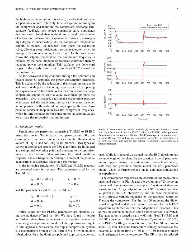
Fig. 6. Extremum seeking decision variable (Td setpt) and objective (power)as explicit functions of time for TV-ESC (blue) and PI-ESC (red) algorithms.Adaptation is turned on at t = 60 min. PI-ESC converges to minimum powerin about 60 min. The ambient air temperature is rapidly increased from 35to 40◦C at t = 610 min and the new optimal Td setpoint is discovered on asimilar timescale.

map. While it is generally assumed that the ESC algorithm hasno knowledge of the plant, for the practical issue of parametertuning, approximating the system time constant and steadystate map can provide a simple model for ESC parametertuning, which is further refined on in nonlinear simulationsor experiments.

The convergence trajectories are overlaid on the steady statemaps and shown in Fig. 5, and the evolution of Td setpoint,power and zone temperature as explicit functions of time areshown in Fig. 6. Td setpoint is the ESC decision variableuk, power is the ESC objective yk, and the zone temperatureTr is a process variable regulated by the feedback controllerK using the compressor. For the first 60 minutes, the dithersignal is applied and the estimation equations for each ESCalgorithm are turned on, but the adaptation is disabled. Thisallows the estimator states to settle before control is activated.The adaptation is turned on at t = 60 min. Both TV-ESC andPI-ESC converge to the optimal inputs Td setpoint = 55.5◦C,with PI-ESC settling in about 60 min, and TV-ESC settling inabout 120 min. The zone temperature initially decreases as thelowered Td setpoint from t = 60 to t = 180 introduces morecool refrigerant into the evaporator. The CF is then be reduced

8 IEEE TRANSACTIONS ON CONTROL SYSTEMS TECHNOLOGY, VOL. XX, NO. YY, MONTH YYYY

108096085

520

84080 72075

560

60070 48065360

600

6024055

12050

640

045

680720760

Time (min)

Pow

er (W

)

Td Setpt (C)

Time-varying ESCProportional-Integral ESCSteady-state maps

Map T amb =

35ºC

Map T amb =

40ºC

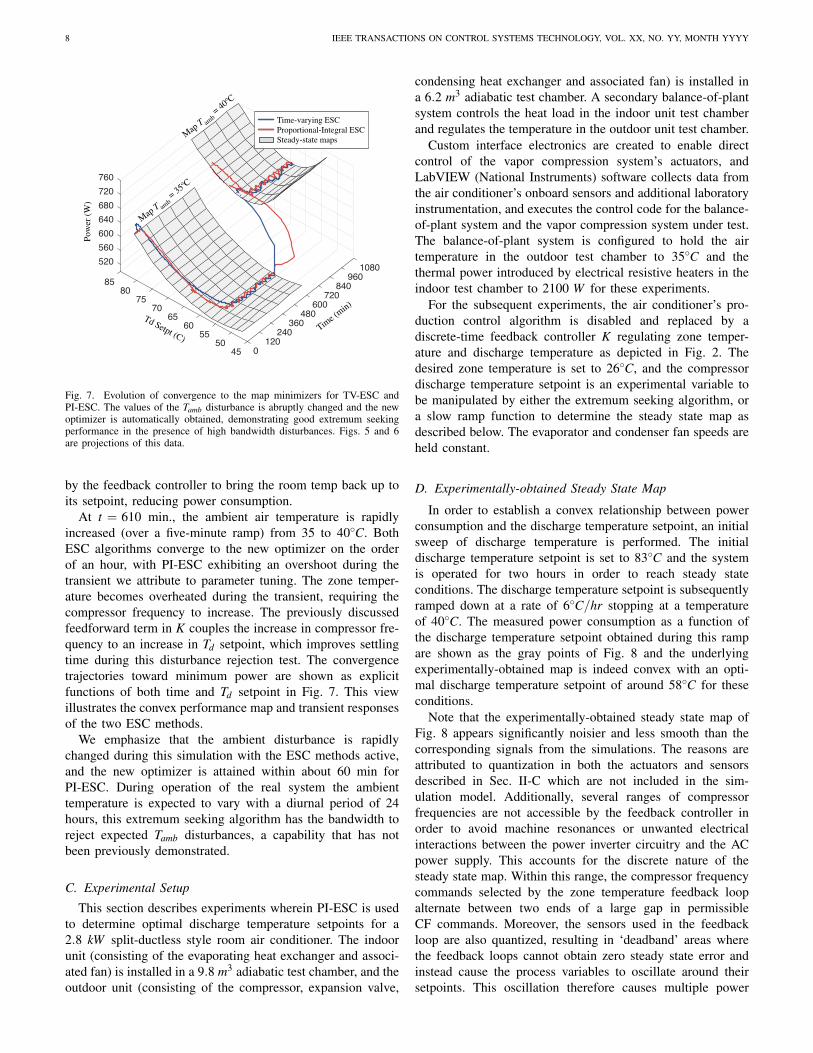
Fig. 7. Evolution of convergence to the map minimizers for TV-ESC andPI-ESC. The values of the Tamb disturbance is abruptly changed and the newoptimizer is automatically obtained, demonstrating good extremum seekingperformance in the presence of high bandwidth disturbances. Figs. 5 and 6are projections of this data.

by the feedback controller to bring the room temp back up toits setpoint, reducing power consumption.

At t = 610 min., the ambient air temperature is rapidlyincreased (over a five-minute ramp) from 35 to 40◦C. BothESC algorithms converge to the new optimizer on the orderof an hour, with PI-ESC exhibiting an overshoot during thetransient we attribute to parameter tuning. The zone temper-ature becomes overheated during the transient, requiring thecompressor frequency to increase. The previously discussedfeedforward term in K couples the increase in compressor fre-quency to an increase in Td setpoint, which improves settlingtime during this disturbance rejection test. The convergencetrajectories toward minimum power are shown as explicitfunctions of both time and Td setpoint in Fig. 7. This viewillustrates the convex performance map and transient responsesof the two ESC methods.

We emphasize that the ambient disturbance is rapidlychanged during this simulation with the ESC methods active,and the new optimizer is attained within about 60 min forPI-ESC. During operation of the real system the ambienttemperature is expected to vary with a diurnal period of 24hours, this extremum seeking algorithm has the bandwidth toreject expected Tamb disturbances, a capability that has notbeen previously demonstrated.

C. Experimental Setup

This section describes experiments wherein PI-ESC is usedto determine optimal discharge temperature setpoints for a2.8 kW split-ductless style room air conditioner. The indoorunit (consisting of the evaporating heat exchanger and associ-ated fan) is installed in a 9.8 m3 adiabatic test chamber, and theoutdoor unit (consisting of the compressor, expansion valve,

condensing heat exchanger and associated fan) is installed ina 6.2 m3 adiabatic test chamber. A secondary balance-of-plantsystem controls the heat load in the indoor unit test chamberand regulates the temperature in the outdoor unit test chamber.

Custom interface electronics are created to enable directcontrol of the vapor compression system’s actuators, andLabVIEW (National Instruments) software collects data fromthe air conditioner’s onboard sensors and additional laboratoryinstrumentation, and executes the control code for the balance-of-plant system and the vapor compression system under test.The balance-of-plant system is configured to hold the airtemperature in the outdoor test chamber to 35◦C and thethermal power introduced by electrical resistive heaters in theindoor test chamber to 2100 W for these experiments.

For the subsequent experiments, the air conditioner’s pro-duction control algorithm is disabled and replaced by adiscrete-time feedback controller K regulating zone temper-ature and discharge temperature as depicted in Fig. 2. Thedesired zone temperature is set to 26◦C, and the compressordischarge temperature setpoint is an experimental variable tobe manipulated by either the extremum seeking algorithm, ora slow ramp function to determine the steady state map asdescribed below. The evaporator and condenser fan speeds areheld constant.

D. Experimentally-obtained Steady State Map

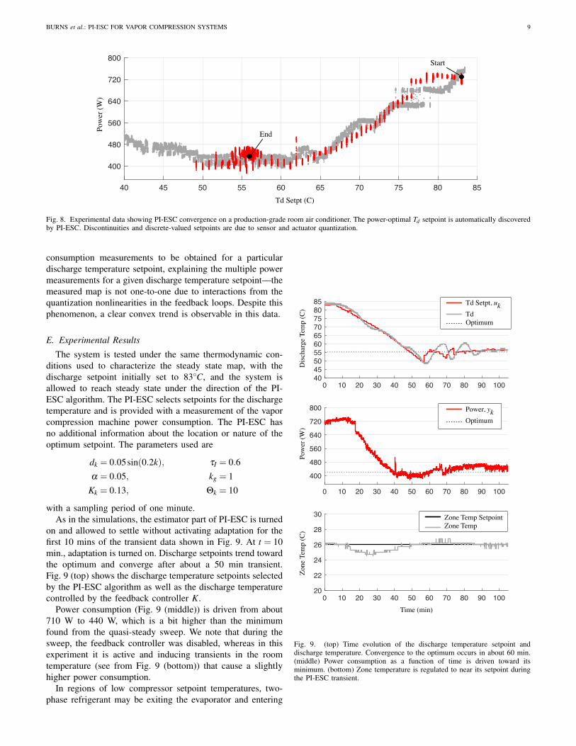
In order to establish a convex relationship between powerconsumption and the discharge temperature setpoint, an initialsweep of discharge temperature is performed. The initialdischarge temperature setpoint is set to 83◦C and the systemis operated for two hours in order to reach steady stateconditions. The discharge temperature setpoint is subsequentlyramped down at a rate of 6◦C/hr stopping at a temperatureof 40◦C. The measured power consumption as a function ofthe discharge temperature setpoint obtained during this rampare shown as the gray points of Fig. 8 and the underlyingexperimentally-obtained map is indeed convex with an opti-mal discharge temperature setpoint of around 58◦C for theseconditions.

Note that the experimentally-obtained steady state map ofFig. 8 appears significantly noisier and less smooth than thecorresponding signals from the simulations. The reasons areattributed to quantization in both the actuators and sensorsdescribed in Sec. II-C which are not included in the sim-ulation model. Additionally, several ranges of compressorfrequencies are not accessible by the feedback controller inorder to avoid machine resonances or unwanted electricalinteractions between the power inverter circuitry and the ACpower supply. This accounts for the discrete nature of thesteady state map. Within this range, the compressor frequencycommands selected by the zone temperature feedback loopalternate between two ends of a large gap in permissibleCF commands. Moreover, the sensors used in the feedbackloop are also quantized, resulting in ‘deadband’ areas wherethe feedback loops cannot obtain zero steady state error andinstead cause the process variables to oscillate around theirsetpoints. This oscillation therefore causes multiple power

BURNS et al.: PI-ESC FOR VAPOR COMPRESSION SYSTEMS 9

40 45 50 55 60 65 70 75 80 85

400

480

560

640

720

800 Start

EndPow

er (W

)

Td Setpt (C)

Fig. 8. Experimental data showing PI-ESC convergence on a production-grade room air conditioner. The power-optimal Td setpoint is automatically discoveredby PI-ESC. Discontinuities and discrete-valued setpoints are due to sensor and actuator quantization.

consumption measurements to be obtained for a particulardischarge temperature setpoint, explaining the multiple powermeasurements for a given discharge temperature setpoint—themeasured map is not one-to-one due to interactions from thequantization nonlinearities in the feedback loops. Despite thisphenomenon, a clear convex trend is observable in this data.

E. Experimental Results

The system is tested under the same thermodynamic con-ditions used to characterize the steady state map, with thedischarge setpoint initially set to 83◦C, and the system isallowed to reach steady state under the direction of the PI-ESC algorithm. The PI-ESC selects setpoints for the dischargetemperature and is provided with a measurement of the vaporcompression machine power consumption. The PI-ESC hasno additional information about the location or nature of theoptimum setpoint. The parameters used are

dk = 0.05sin(0.2k), τI = 0.6α = 0.05, kg = 1

Kk = 0.13, Θk = 10

with a sampling period of one minute.As in the simulations, the estimator part of PI-ESC is turned

on and allowed to settle without activating adaptation for thefirst 10 mins of the transient data shown in Fig. 9. At t = 10min., adaptation is turned on. Discharge setpoints trend towardthe optimum and converge after about a 50 min transient.Fig. 9 (top) shows the discharge temperature setpoints selectedby the PI-ESC algorithm as well as the discharge temperaturecontrolled by the feedback controller K.

Power consumption (Fig. 9 (middle)) is driven from about710 W to 440 W, which is a bit higher than the minimumfound from the quasi-steady sweep. We note that during thesweep, the feedback controller was disabled, whereas in thisexperiment it is active and inducing transients in the roomtemperature (see from Fig. 9 (bottom)) that cause a slightlyhigher power consumption.

In regions of low compressor setpoint temperatures, two-phase refrigerant may be exiting the evaporator and entering

0 10 20 30 40 50 60 70 80 90 10040455055606570758085

0 10 20 30 40 50 60 70 80 90 100

400

480

560

640

720

800

0 10 20 30 40 50 60 70 80 90 10020

22

24

26

28

30

Time (min)

Td Setpt, ukTdOptimum

Pow

er (W

)D

ischa

rge

Tem

p (C

)Zo

ne T

emp

(C)

Power, ykOptimum

Zone Temp SetpointZone Temp

Fig. 9. (top) Time evolution of the discharge temperature setpoint anddischarge temperature. Convergence to the optimum occurs in about 60 min.(middle) Power consumption as a function of time is driven toward itsminimum. (bottom) Zone temperature is regulated to near its setpoint duringthe PI-ESC transient.

10 IEEE TRANSACTIONS ON CONTROL SYSTEMS TECHNOLOGY, VOL. XX, NO. YY, MONTH YYYY

the compressor, potentially damaging the compressor if thiscondition is allowed to persist for too long. Consequently, theprojection operator parameter Θk is selected to limit the rate ofchange of the setpoint in order to eliminate overshoot that mayhave caused excessively low setpoint values and potentiallydamaging liquid refrigerant ingestion. Projecting the estimatedparameters θ back into the constraint set therefore serves as animportant feature for practical problems where regions of thestate space must be avoided for equipment protection. In futurework, explicit constraints on the ESC decision variables willbe considered, which will require reformulating the estimatorfor bumpless transition as constraints become active.

V. CONCLUSION

We have applied a novel proportional-integral extremumseeking algorithm to energy-optimal setpoint selection fora vapor compression system. The rapid convergence prop-erties of the PI-ESC algorithm are especially attractive forvapor compression systems because the relative bandwidthsof disturbance rejection of the closed loop system and typicaldisturbances are such that the system is rarely in equilibriumfor periods to satisfy the two timescale separation requirementof traditional perturbation-based ESC. We have demonstratedthe improved convergence properties of PI-ESC relative toother methods on an example problem, and used a physics-based model with realistic disturbance properties to show ap-plicability of extremum seeking to vapor compression systems.Finally, we have validated the approach in an experimentalscenario where noise and actuator and sensor quantization aresignificant.

Daniel J. Burns (M’10-SM’18) Daniel Burns re-ceived the M.S. and Ph.D. degrees in mechanical en-gineering from the Massachusetts Institute of Tech-nology, Cambridge, in 2006 and 2010, respectively.Since 2010, he has been with Mitsubishi ElectricResearch Laboratories (MERL), Cambridge, MA,where he is a Senior Principal Research Scientist. AtMERL, Dr. Burns develops and prototypes advancedcontrol methods for vapor compression systems.Before joining MERL, he worked on flight instru-mentation and control at the Commercial Aviation

Systems division of Honeywell, Inc. (Phoenix, AZ) and NASA’s GoddardSpace Flight Center (Greenbelt, MD). At MIT, he designed and built mecha-nisms and controllers for high-speed atomic force microscopes. His researchinterests include multi-physical modeling and control of mechatronic andthermodynamic systems, instrumentation and experimentation, and appliedpredictive and adaptive control.

Christopher R. Laughman Chris Laughman is aSenior Principal Research Scientist at MitsubishiElectric Research Labs investigating the model-ing, simulation, control, and optimization of large-scale multiphysical systems. He obtained his Ph.D.in Building Technology at MIT in 2008, and iscurrently focused on the development of high-performance and energy-efficient building systems.

Martin Guay Martin Guay is a Professor in theDepartment of Chemical Engineering at Queen’sUniversity in Kingston, Ontario, Canada. He re-ceived his PhD from Queen’s University in 1996.Dr. Guay is Senior Editor for the IEEE CSS Let-ters. He is deputy Editor-in-Chief of the Journalof Process Control. He is also an associate editorfor Automatica, IEEE Transactions on AutomaticControl, Canadian Journal of Chemical Engineeringand Nonlinear Analysis & Hybrid Systems. He wasthe recipient of the Syncrude Innovation award and

the D.G. Fisher from the Canadian Society of Chemical Engineers. He alsoreceived the Premier Research Excellence award. His research interests are inthe area of nonlinear control systems including extremum-seeking control,nonlinear model predictive control, adaptive estimation and control, andgeometric control.

REFERENCES

[1] K. J. Chua, S. K. Chou, and W. M. Yang, “Advances in heat pumpsystems: A review,” Applied Energy, vol. 87, no. 12, pp. 3611–3624,Dec 2010.

[2] A. Hepbasli and Y. Kalinci, “A review of heat pump water heatingsystems,” Renewable and Sustainable Energy Reviews, vol. 13, no. 6–7,pp. 1211 – 1229, 2009.

[3] S. A. Tassou, G. De-Lille, and Y. T. Ge, “Food transport refrigeration—Approaches to reduce energy consumption and environmental impactsof road transport,” Applied Thermal Engineering, vol. 29, no. 8-9, pp.1467–1477, Jun 2009.

[4] V. Slesarenko, “Heat pumps as a source of heat energy for desalinationof seawater,” Desalination, vol. 139, no. 1–3, pp. 405 – 410, 2001.

[5] J. Burger, H. Holland, E. Berenschot, J. Seppenwodde, M. ter Brake,H. Gardeniers, and M. Elwenspoek, “169 Kelvin cryogenic microcooleremploying a condenser, evaporator, flow restriction and counterflow heatexchangers,” in 14th IEEE International Conference On Micro ElectroMechanical Systems, 2001, pp. 418–421.

[6] R. J. Otten, “Superheat control for air conditioning and refrigerationsystems: Simulation and experiments,” Master’s thesis, University ofIllinois at Urbana-Champaign, 2010.

[7] M. S. Elliott and B. P. Rasmussen, “On reducing evaporator superheatnonlinearity with control architecture,” International Journal of Refrig-eration, vol. 33, no. 3, pp. 607–614, 2010.

[8] K. Vinther, H. Rasmussen, R. Izadi-Zamanabadi, and J. Stoustrup,“Single temperature sensor superheat control using a novel maximumslope-seeking method,” International Journal of Refrigeration, vol. 36,no. 3, pp. 1118–1129, 2013.

[9] D. Burns, W. Weiss, and M. Guay, “Realtime setpoint optimizationwith time-varying extremum seeking for vapor compression systems,”in American Control Conference, 2015.

[10] D. Burns and C. Laughman, “Extremum seeking control for energy opti-mization of vapor compression systems,” in International Refrigerationand Air Conditioning Conference, 2012.

[11] M. Guay and D. Burns, “A comparison of extremum seeking algorithmsapplied to vapor compression system optimization,” in American ControlConference, 2014.

[12] H. Sane, C. Haugstetter, and S. Bortoff, “Building HVAC controlsystems—role of controls and optimization,” in American Control Con-ference, 2006.

[13] P. Li, Y. Li, and J. E. Seem, “Efficient Operation of Air-Side Econo-mizer Using Extremum Seeking Control,” Journal of Dynamic Systems,Measurement, and Control, vol. 132, no. 3, May 2010.

[14] V. Tyagi, H. Sane, and S. Darbha, “An extremum seeking algorithm fordetermining the set point temperature for condensed water in a coolingtower,” in American Control Conference, 2006.

[15] M. Leblanc, “Sur l’electrification des chemins de fer au moyende courants alternatifs de frequence elevee,” Revue Generale del’Electricite, 1922.

[16] M. Krstic, “Performance Improvement and Limitations in ExtremumSeeking Control,” Systems & Control Letters, vol. 39, no. 5, pp. 313–326, April 2000.

[17] Y. Tan, W. Moase, C. Manzie, D. Nesic and, and I. Mareels, “Extremumseeking from 1922 to 2010,” in 29th Chinese Control Conference (CCC),2010.

[18] M. Guay, “A time-varying extremum-seeking control approach fordiscrete-time systems,” Journal of Process Control, vol. 24, no. 3, pp.98 – 112, 2014.

BURNS et al.: PI-ESC FOR VAPOR COMPRESSION SYSTEMS 11

[19] M. Guay and D. J. Burns, “A proportional integral extremum-seekingcontrol approach for discrete-time nonlinear systems,” InternationalJournal of Control, vol. 90, no. 8, pp. 1543–1554, 2017.

[20] A. Bejan, Advanced Engineering Thermodynamics, 3rd ed. Wiley, 2006.[21] P. Broersen and M. van der Jagt, “Hunting of evaporators controlled by

a thermostatic expansion valve,” Journal of Dynamic Systems, Measure-ment, and Control, vol. 102, pp. 130–135, 1980.

[22] D. J. Burns, C. Laughman, and S. A. Bortoff, “System and method forcontrolling vapor compression systems,” United States Patent 9,534,820,January 3, 2017.

[23] G. Goodwin and K. Sin, Adaptive Filtering Prediction and Control.Dover Publications, Incorporated, 2013.

[24] N. J. Killingsworth and M. Krstic, “PID tuning using extremum seeking:online, model-free performance optimization,” IEEE Control SystemsMagazine, vol. 26, no. 1, pp. 70–79, Feb. 2006.

[25] Modelica Association. (2015) Modelica specification, version 3.3r1.[Online]. Available: www.modelica.org

[26] C. Laughman, H. Qiao, V. Aute, and R. Radermacher, “A comparison oftransient heat pump cycle models using alternative flow descriptions,”Science and Technology for the Built Environment, vol. 21, no. 5, pp.666–680, 2015.

[27] Dassault Systemes, AB. (2015) Dymola.