Maximum Power Point Tracking for Photovoltaic Optimization

Using Extremum Seeking

Steve Brunton1, Clancy Rowley1, Sanj Kulkarni1, and Charles Clarkson2

1Princeton University2ITT Space Systems Division 34th IEEE PVSC

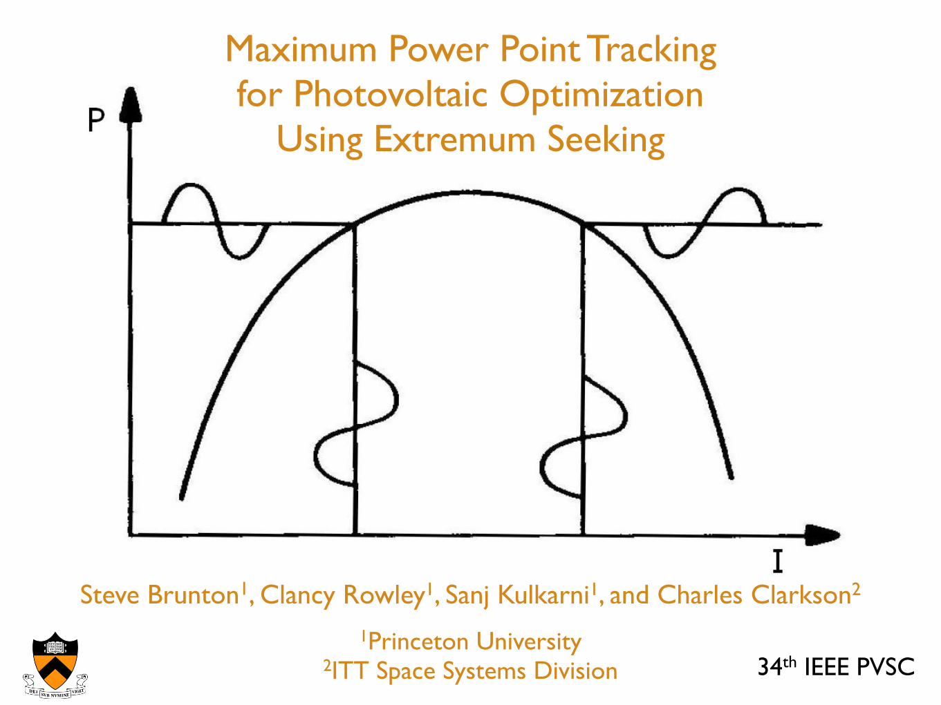
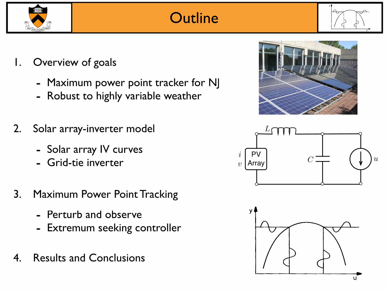
2. Solar array-inverter model

3. Maximum Power Point Tracking

- Perturb and observe- Extremum seeking controller

- Solar array IV curves- Grid-tie inverter

4. Results and Conclusions

Outline

!"#

$%%&'uC

L

iv

1. Overview of goals

- Maximum power point tracker for NJ- Robust to highly variable weather

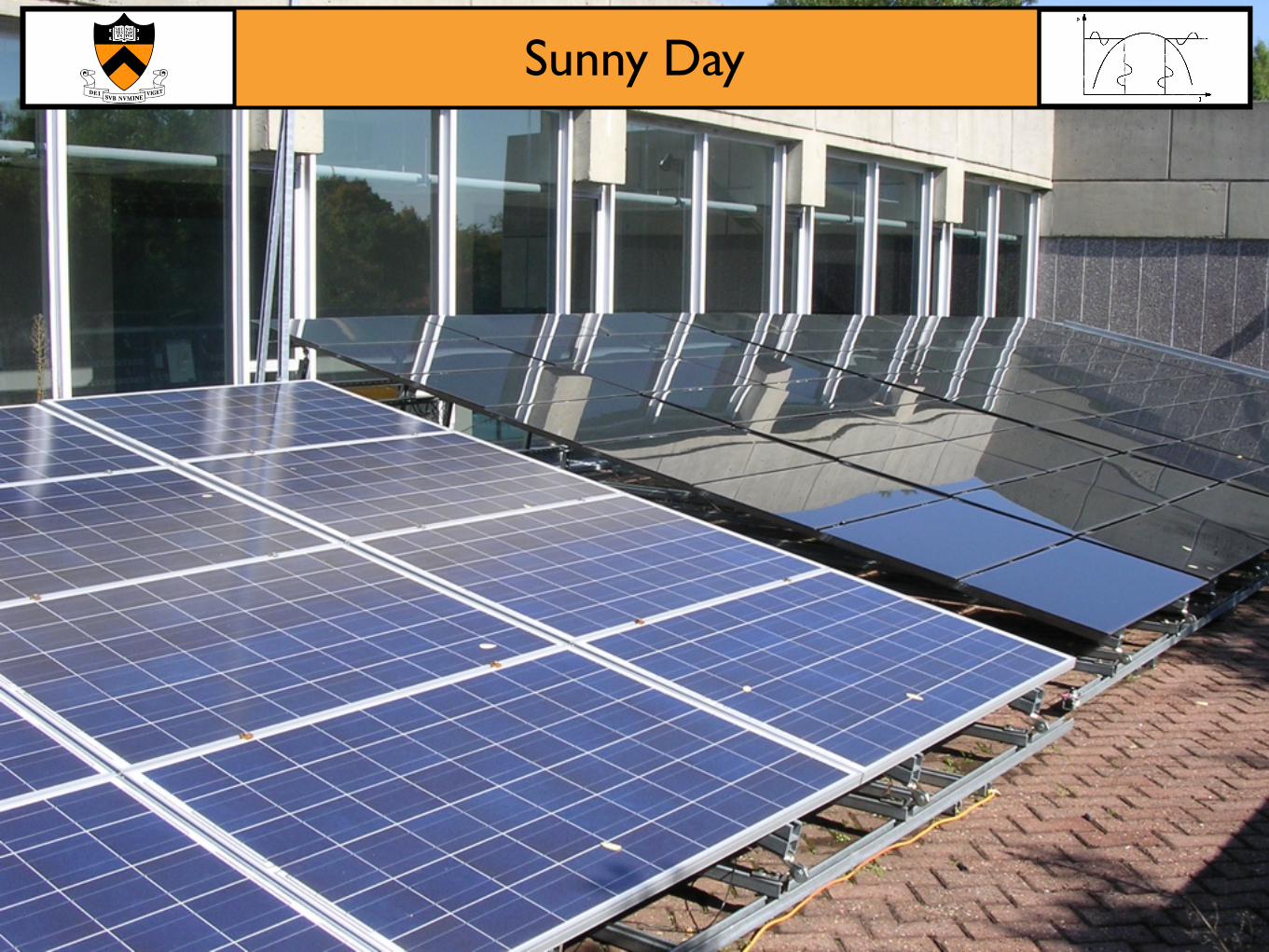
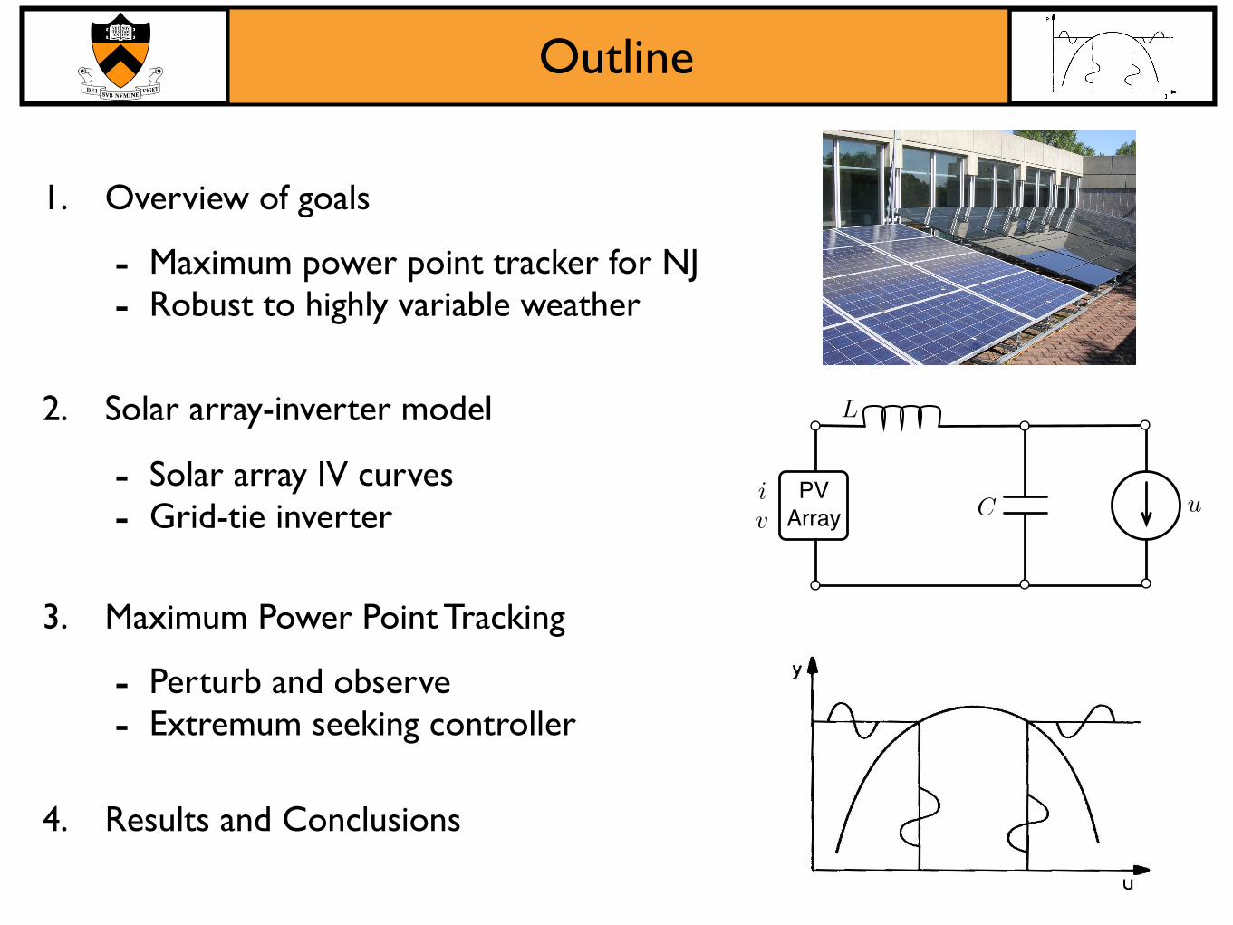
Sunny Day

Cloudy Day

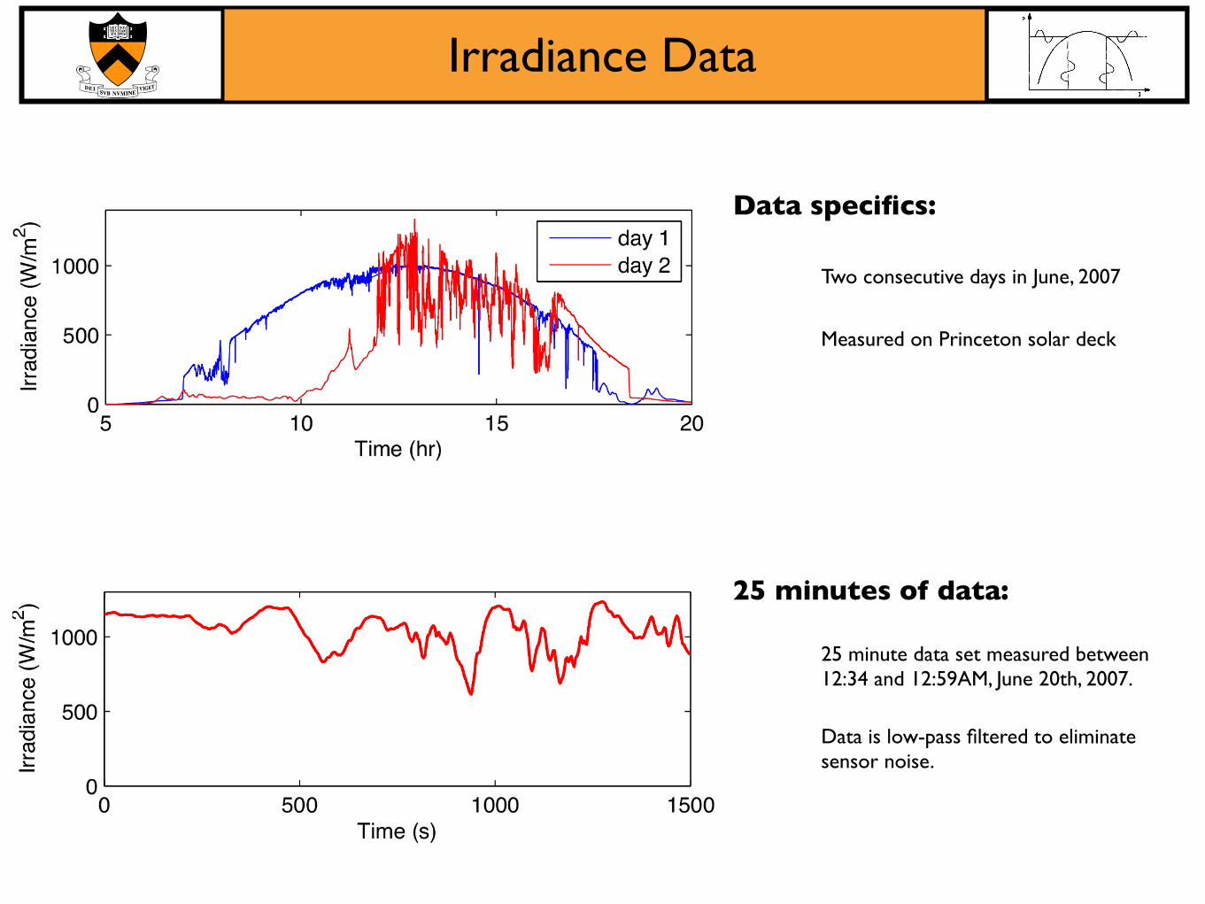
Irradiance Data

Measured on Princeton solar deck

Two consecutive days in June, 2007

Data specifics:

Data is low-pass filtered to eliminate sensor noise.

25 minute data set measured between 12:34 and 12:59AM, June 20th, 2007.

25 minutes of data:

2. Solar array-inverter model

3. Maximum Power Point Tracking

- Perturb and observe- Extremum seeking controller

- Solar array IV curves- Grid-tie inverter

4. Results and Conclusions

Outline

!"#

$%%&'uC

L

iv

1. Overview of goals

- Maximum power point tracker for NJ- Robust to highly variable weather

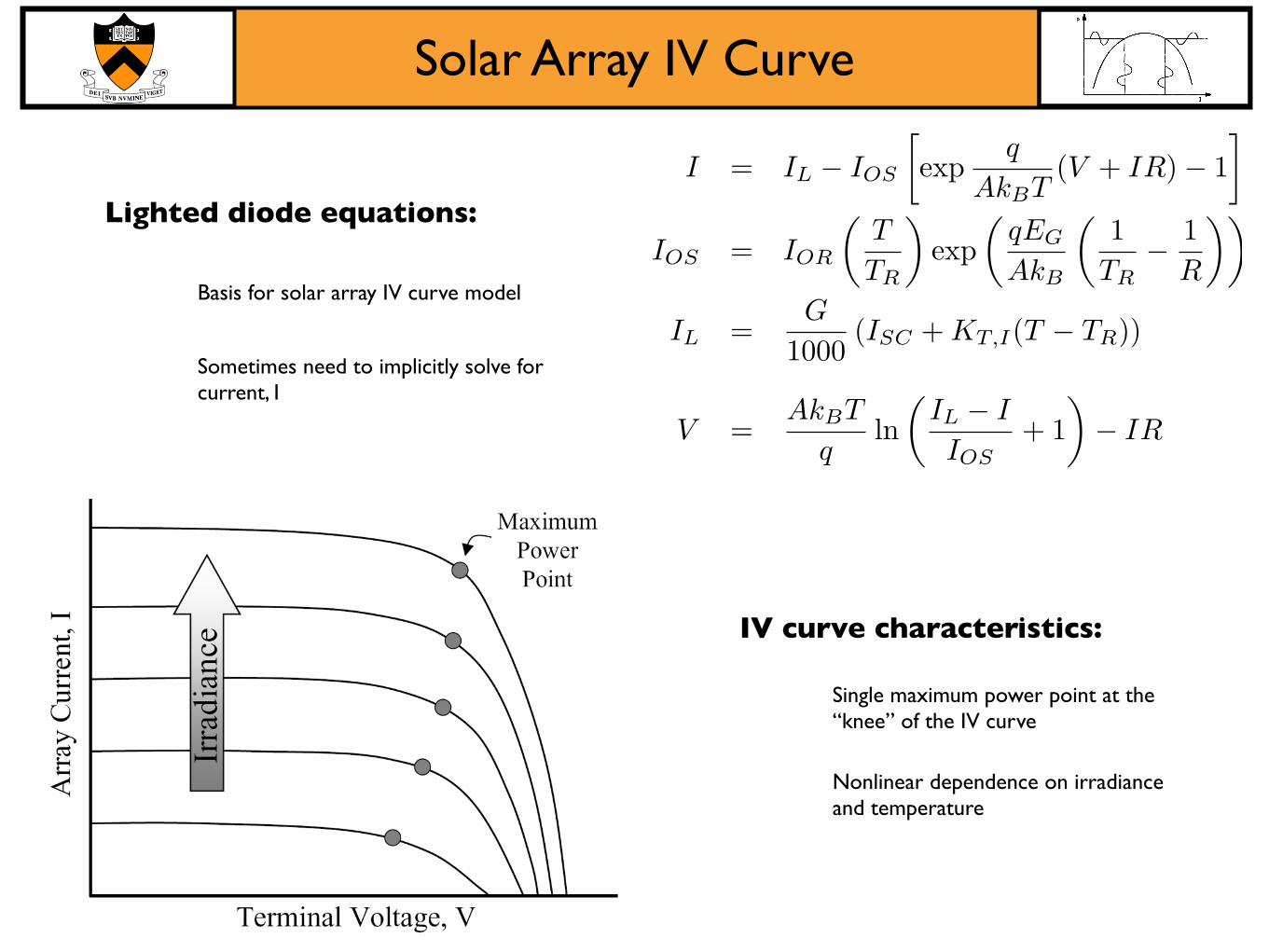
Solar Array IV Curve

I = IL ! IOS

!exp

q

AkBT(V + IR)! 1

"

IOS = IOR

#T

TR

$exp

#qEG

AkB

#1

TR! 1

R

$$

IL =G

1000(ISC + KT,I(T ! TR))

V =AkBT

qln

#IL ! I

IOS+ 1

$! IR

Nonlinear dependence on irradiance and temperature

Single maximum power point at the “knee” of the IV curve

IV curve characteristics:

Sometimes need to implicitly solve for current, I

Basis for solar array IV curve model

Lighted diode equations:

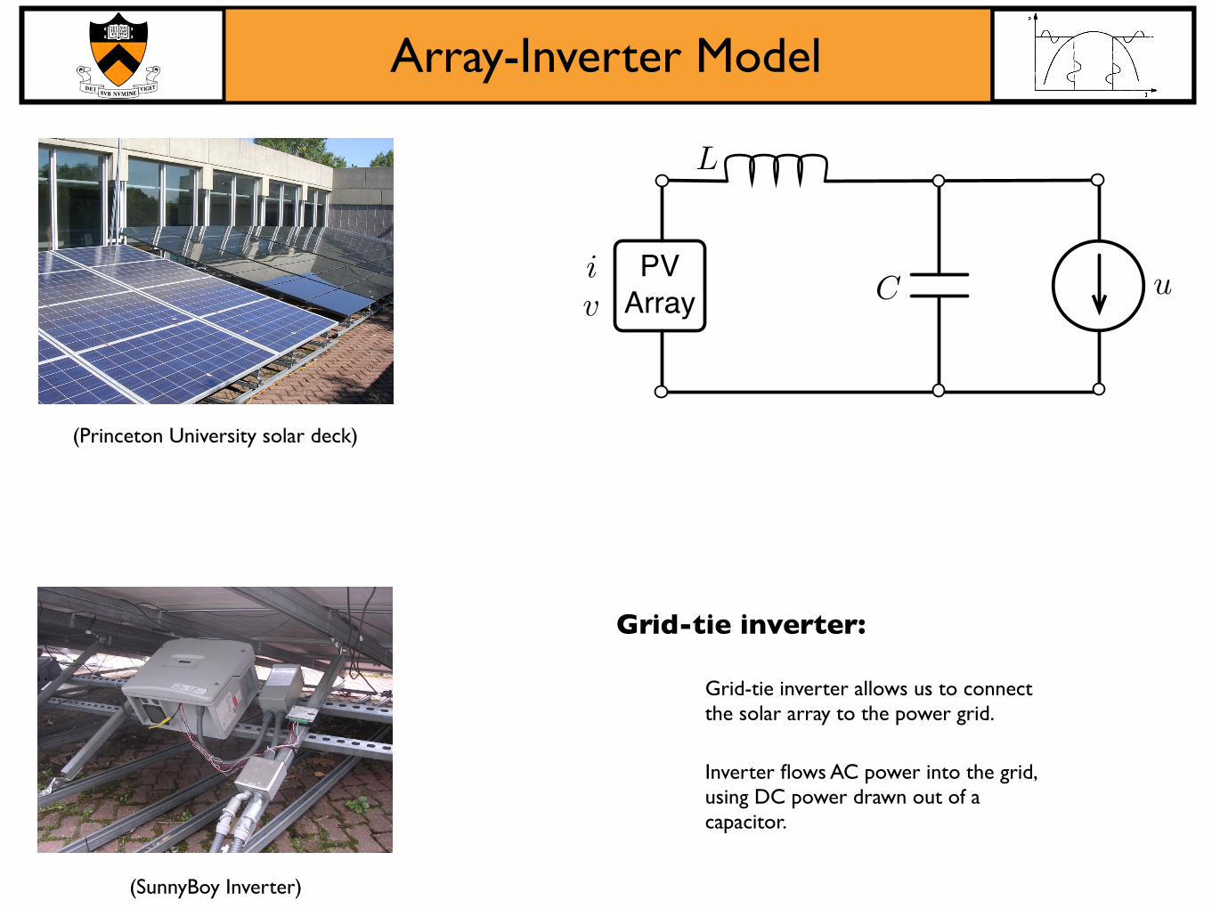
Array-Inverter Model

!"#

$%%&'uC

L

iv

Inverter flows AC power into the grid, using DC power drawn out of a capacitor.

Grid-tie inverter allows us to connect the solar array to the power grid.

Grid-tie inverter:

(Princeton University solar deck)

(SunnyBoy Inverter)

Array-Inverter Model

!"#

$%%&'uC

L

iv

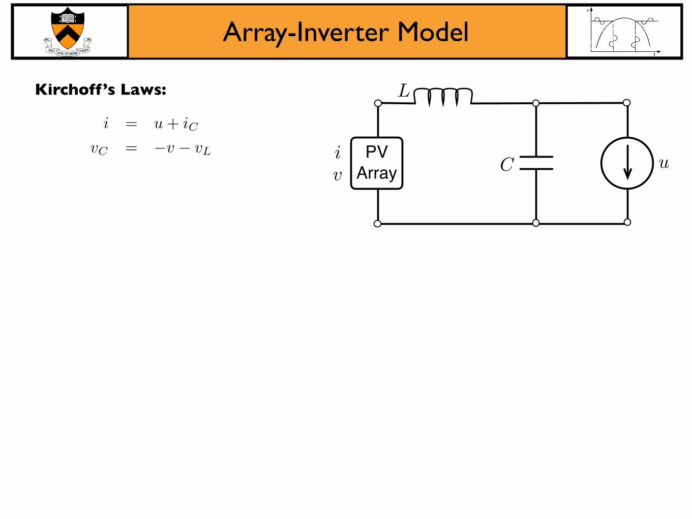
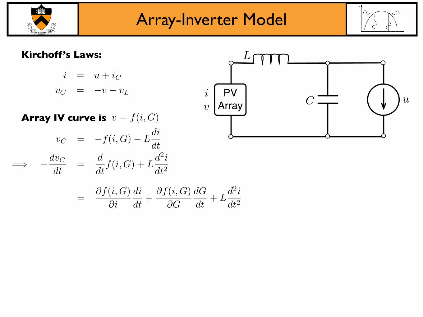
Kirchoff’s Laws:

i = u + iC

vC = !v ! vL

Array-Inverter Model

!"#

$%%&'uC

L

iv

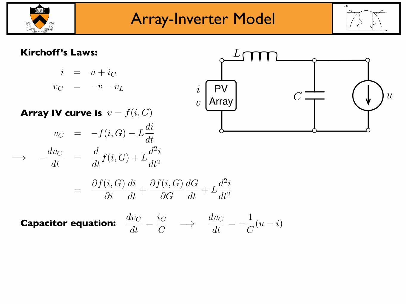
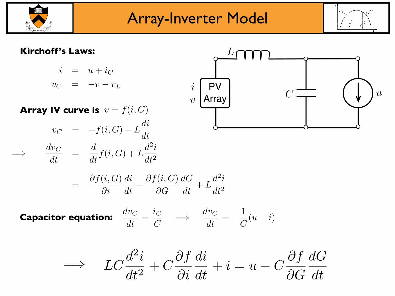
Array IV curve is

Kirchoff’s Laws:

i = u + iC

vC = !v ! vL

vC = !f(i, G)! Ldi

dt

=" !dvC

dt=

d

dtf(i, G) + L

d2i

dt2

=!f(i, G)

!i

di

dt+

!f(i, G)!G

dG

dt+ L

d2i

dt2

v = f(i, G)

Array-Inverter Model

!"#

$%%&'uC

L

iv

Array IV curve is

Kirchoff’s Laws:

i = u + iC

vC = !v ! vL

vC = !f(i, G)! Ldi

dt

=" !dvC

dt=

d

dtf(i, G) + L

d2i

dt2

=!f(i, G)

!i

di

dt+

!f(i, G)!G

dG

dt+ L

d2i

dt2

v = f(i, G)

dvC

dt=

iCC

=! dvC

dt= " 1

C(u" i)Capacitor equation:

Array-Inverter Model

!"#

$%%&'uC

L

iv

Array IV curve is

Kirchoff’s Laws:

i = u + iC

vC = !v ! vL

vC = !f(i, G)! Ldi

dt

=" !dvC

dt=

d

dtf(i, G) + L

d2i

dt2

=!f(i, G)

!i

di

dt+

!f(i, G)!G

dG

dt+ L

d2i

dt2

v = f(i, G)

dvC

dt=

iCC

=! dvC

dt= " 1

C(u" i)Capacitor equation:

LCd2i

dt2+ C

!f

!i

di

dt+ i = u! C

!f

!G

dG

dt=!

2. Solar array-inverter model

3. Maximum Power Point Tracking

- Perturb and observe- Extremum seeking controller

- Solar array IV curves- Grid-tie inverter

4. Results and Conclusions

Outline

!"#

$%%&'uC

L

iv

1. Overview of goals

- Maximum power point tracker for NJ- Robust to highly variable weather

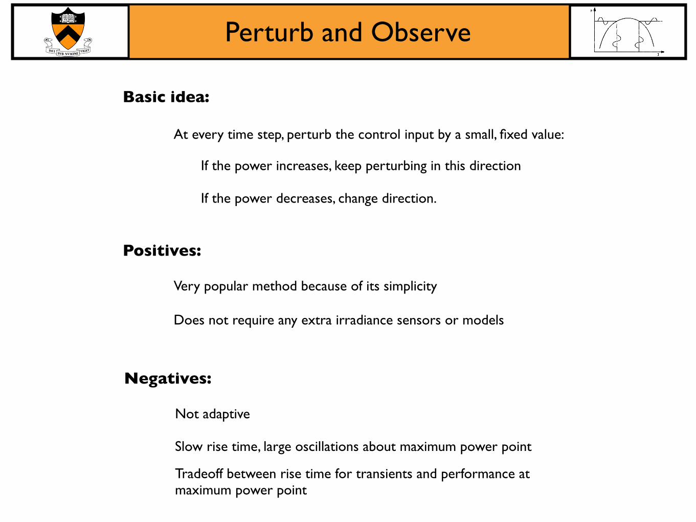
Perturb and Observe

At every time step, perturb the control input by a small, fixed value:

Basic idea:

If the power increases, keep perturbing in this direction

If the power decreases, change direction.

Very popular method because of its simplicity

Does not require any extra irradiance sensors or models

Positives:

Not adaptive

Slow rise time, large oscillations about maximum power point

Negatives:

Tradeoff between rise time for transients and performance at maximum power point

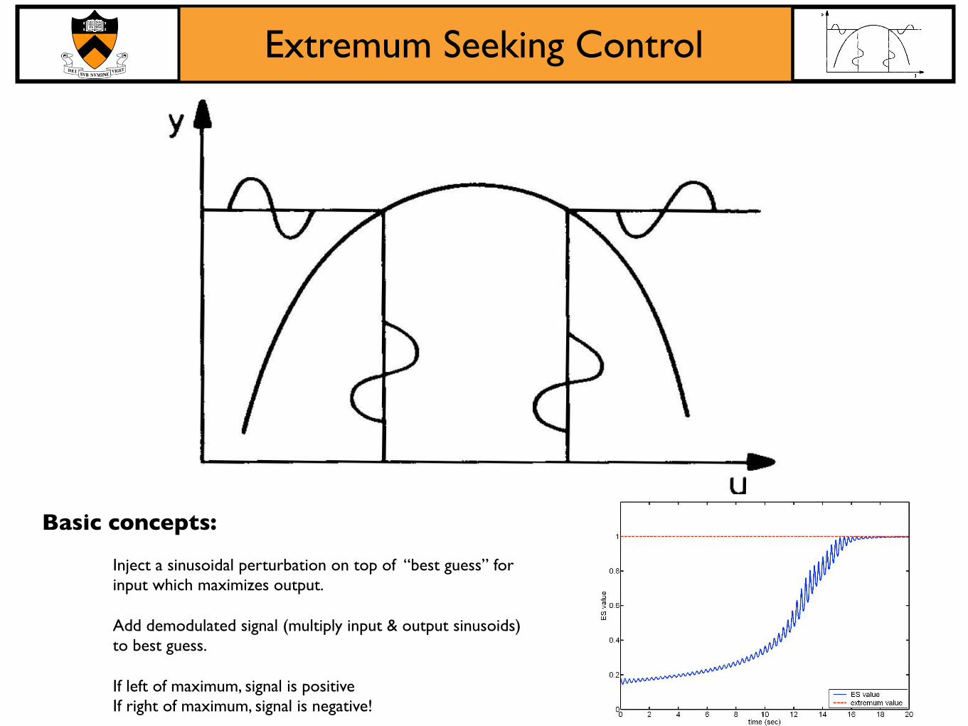
Extremum Seeking Control

Inject a sinusoidal perturbation on top of “best guess” for input which maximizes output.

Basic concepts:

Add demodulated signal (multiply input & output sinusoids)to best guess.

If left of maximum, signal is positiveIf right of maximum, signal is negative!

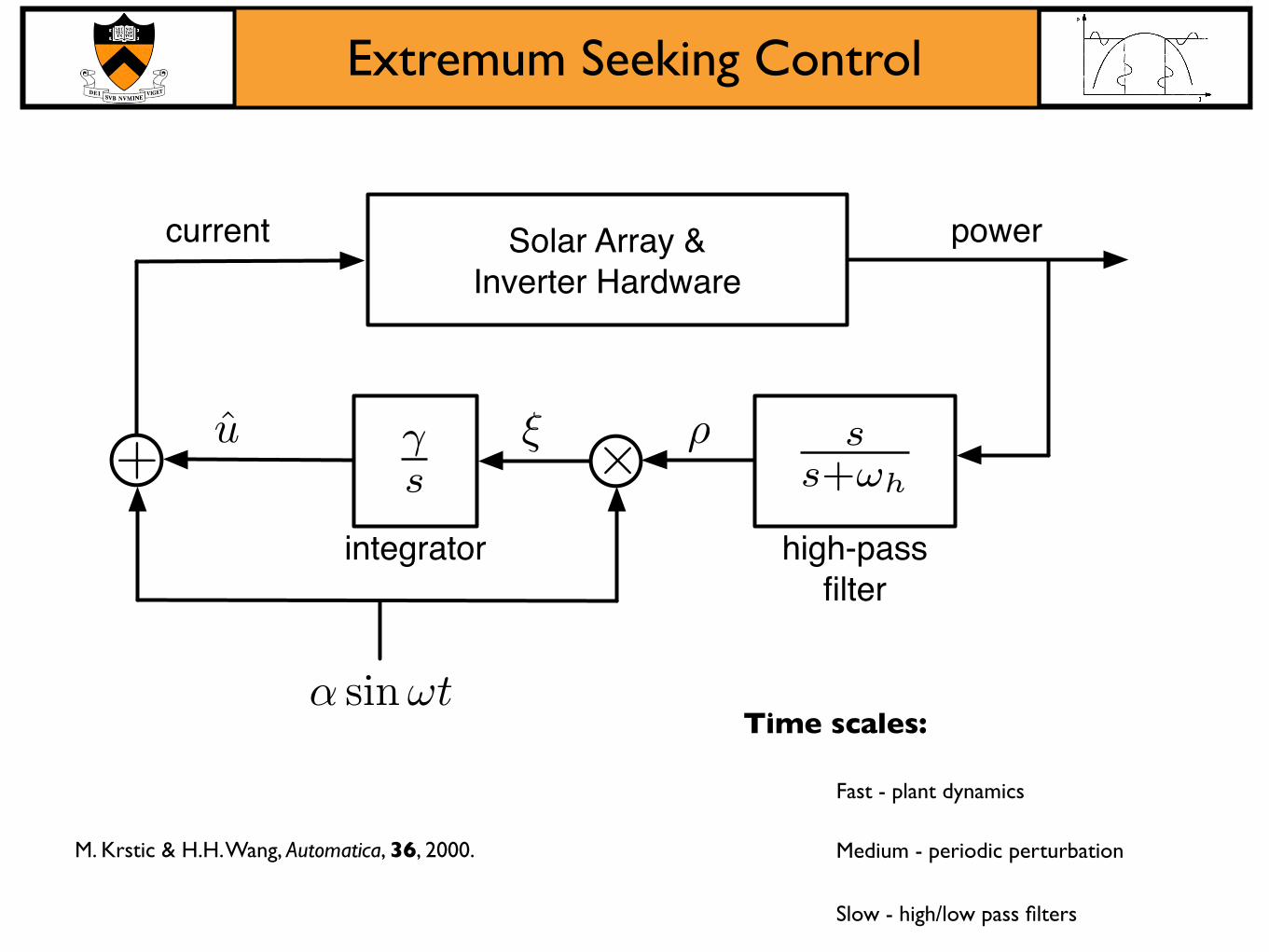
Extremum Seeking Control

!"#$%&'%%$(&)

*+,-%.-%&/$%01$%-

ss+!h

"s !+

23%%-+. 4"1-%

567584$99&

!#.-%

6+.-7%$."%

!"

# sin $t

u

M. Krstic & H.H. Wang, Automatica, 36, 2000. Medium - periodic perturbation

Fast - plant dynamics

Time scales:

Slow - high/low pass filters

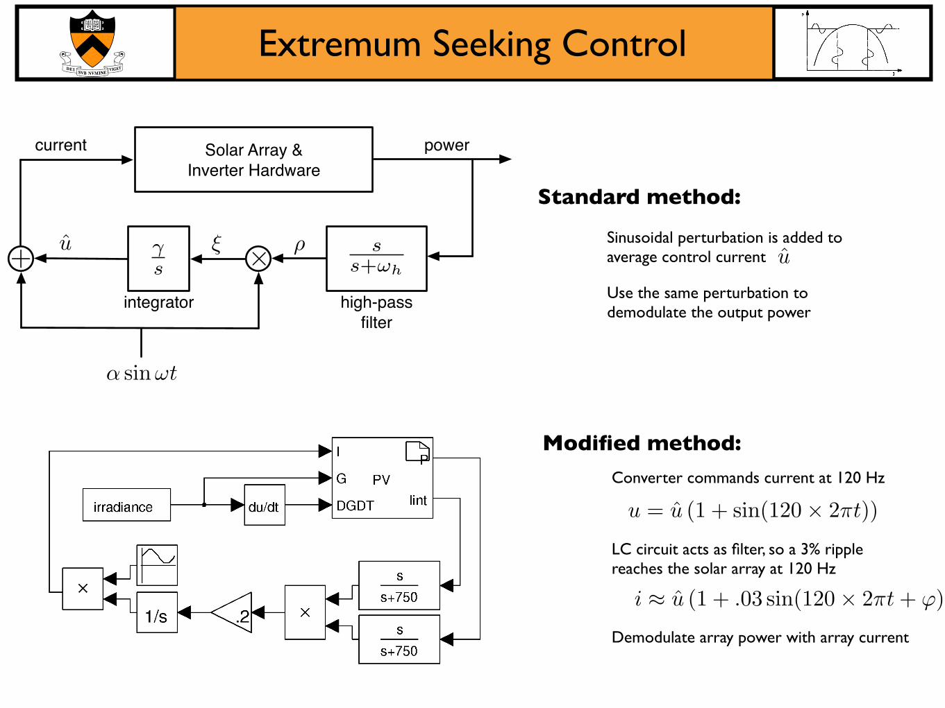
Extremum Seeking Control

!"#$%&'%%$(&)

*+,-%.-%&/$%01$%-

ss+!h

"s !+

23%%-+. 4"1-%

567584$99&

!#.-%

6+.-7%$."%

!"

# sin $t

u

Use the same perturbation to demodulate the output power

Standard method:

Sinusoidal perturbation is added to average control current u

Demodulate array power with array current

Modified method:

LC circuit acts as filter, so a 3% ripple reaches the solar array at 120 Hz

u = u (1 + sin(120! 2!t))

i ! u (1 + .03 sin(120" 2!t + "))

Converter commands current at 120 Hz

2. Solar array-inverter model

3. Maximum Power Point Tracking

- Perturb and observe- Extremum seeking controller

- Solar array IV curves- Grid-tie inverter

4. Results and Conclusions

Outline

!"#

$%%&'uC

L

iv

1. Overview of goals

- Maximum power point tracker for NJ- Robust to highly variable weather

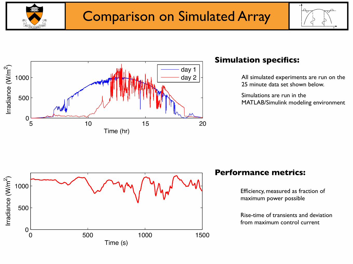
Comparison on Simulated Array

Simulations are run in the MATLAB/Simulink modeling environment

All simulated experiments are run on the 25 minute data set shown below.

Simulation specifics:

Rise-time of transients and deviation from maximum control current

Efficiency, measured as fraction of maximum power possible

Performance metrics:

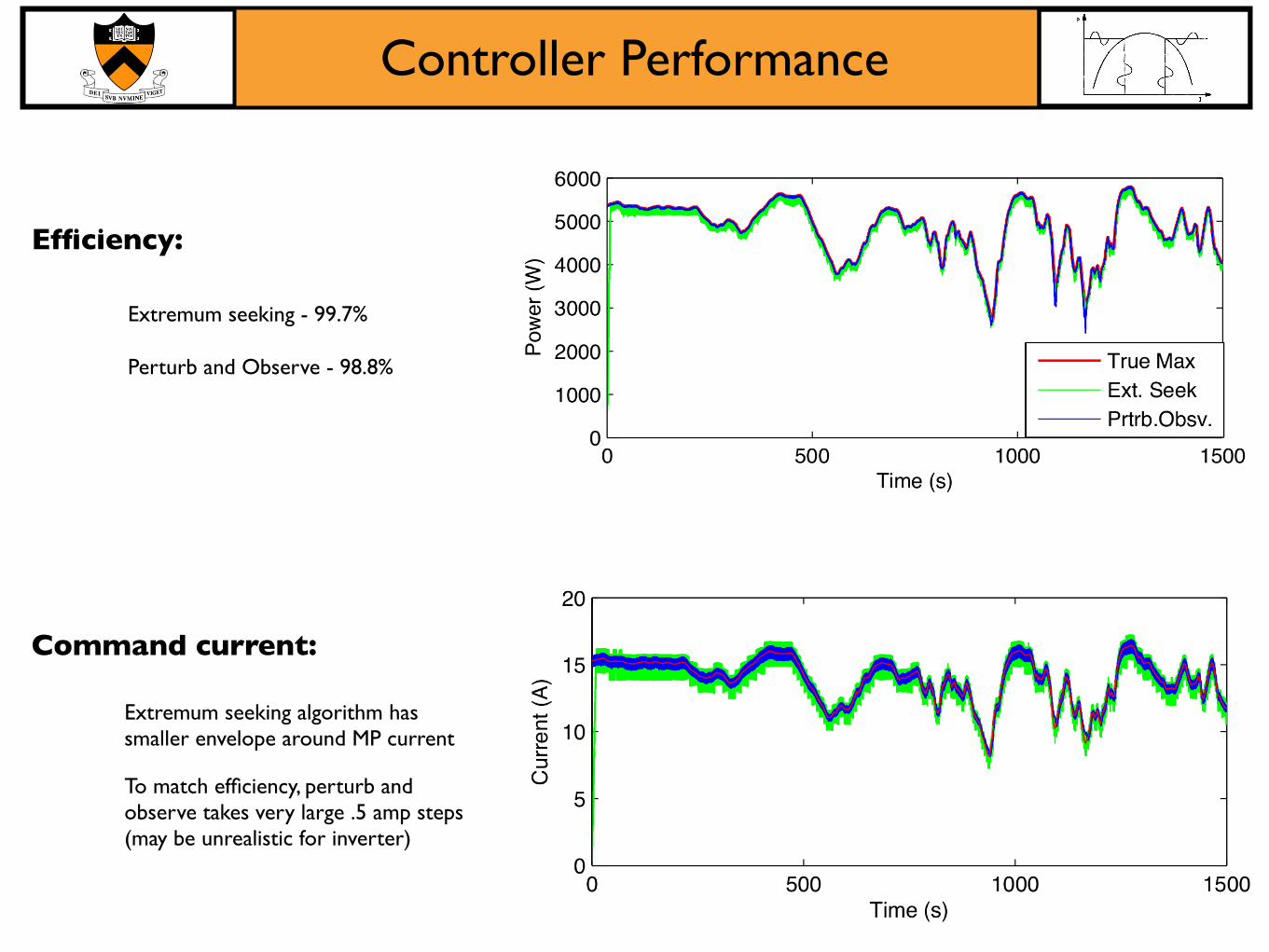
Controller Performance

Perturb and Observe - 98.8%

Extremum seeking - 99.7%

Efficiency:

To match efficiency, perturb and observe takes very large .5 amp steps(may be unrealistic for inverter)

Extremum seeking algorithm has smaller envelope around MP current

Command current:

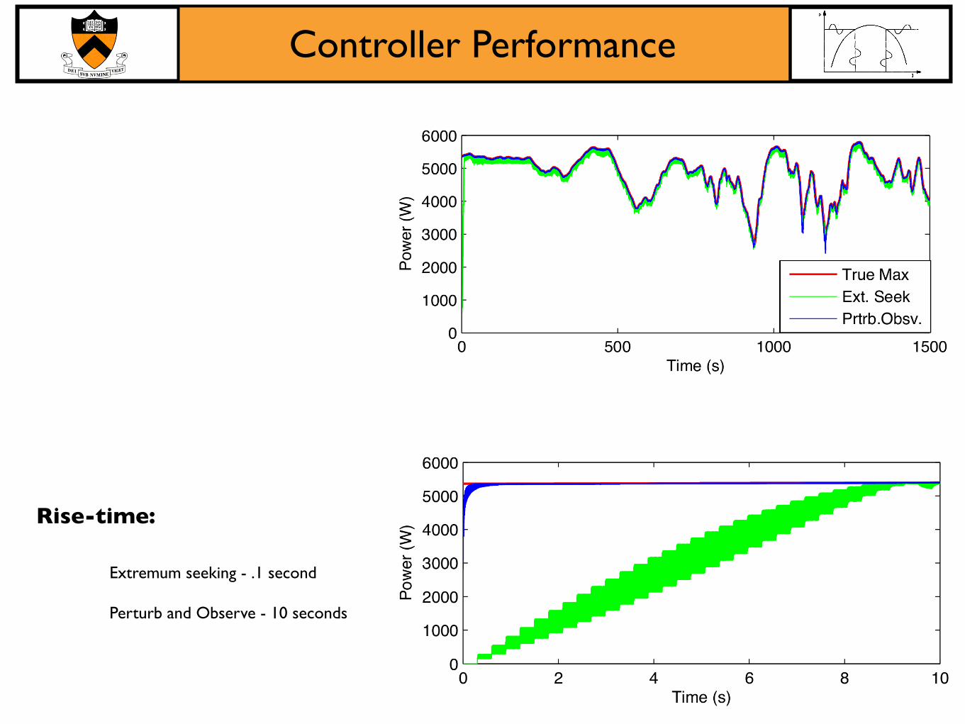
Controller Performance

Perturb and Observe - 10 seconds

Extremum seeking - .1 second

Rise-time:

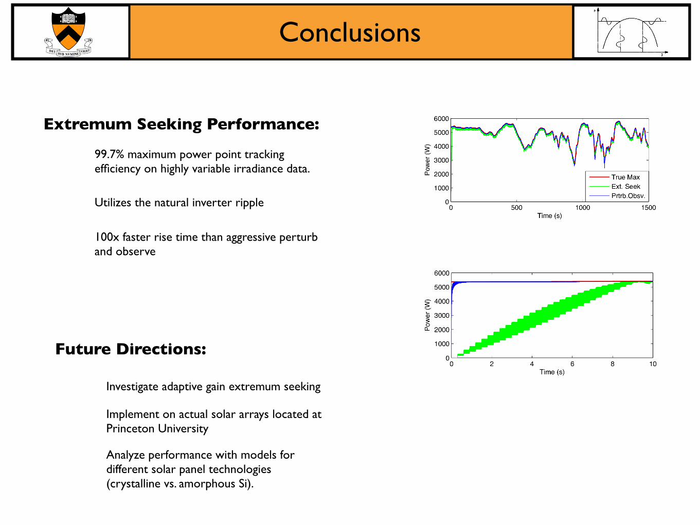
Conclusions

Utilizes the natural inverter ripple

Extremum Seeking Performance:

99.7% maximum power point tracking efficiency on highly variable irradiance data.

100x faster rise time than aggressive perturb and observe

Implement on actual solar arrays located at Princeton University

Future Directions:

Investigate adaptive gain extremum seeking

Analyze performance with models for different solar panel technologies(crystalline vs. amorphous Si).

Acknowledgments

Princeton Power Systems

- Mark Holveck- Erik Limpaecher- Frank Hoffmann- Swarnab Banerjee

EPV Solar

- Alan Delahoy- Loan Le

New Jersey Commission on Science and Technology (NJCST)

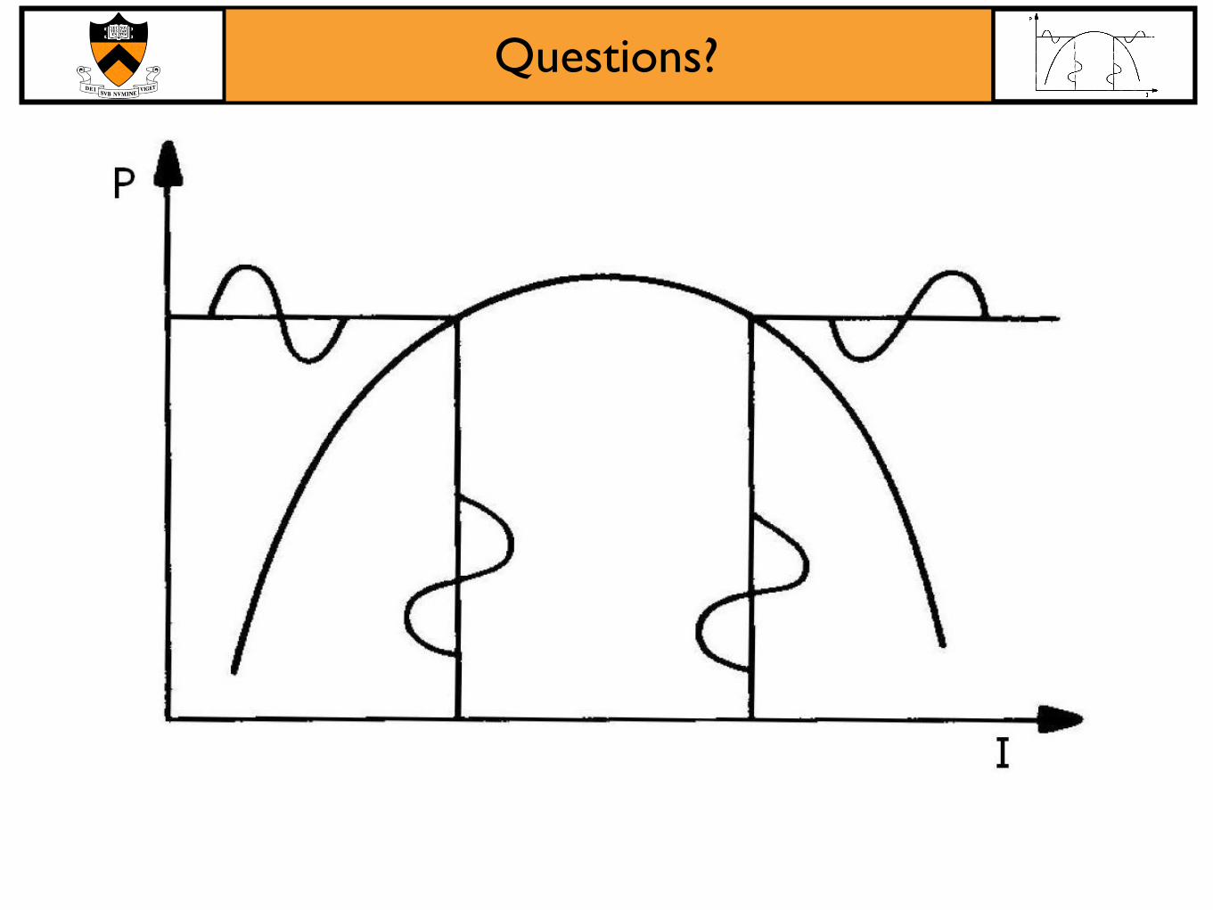
Questions?

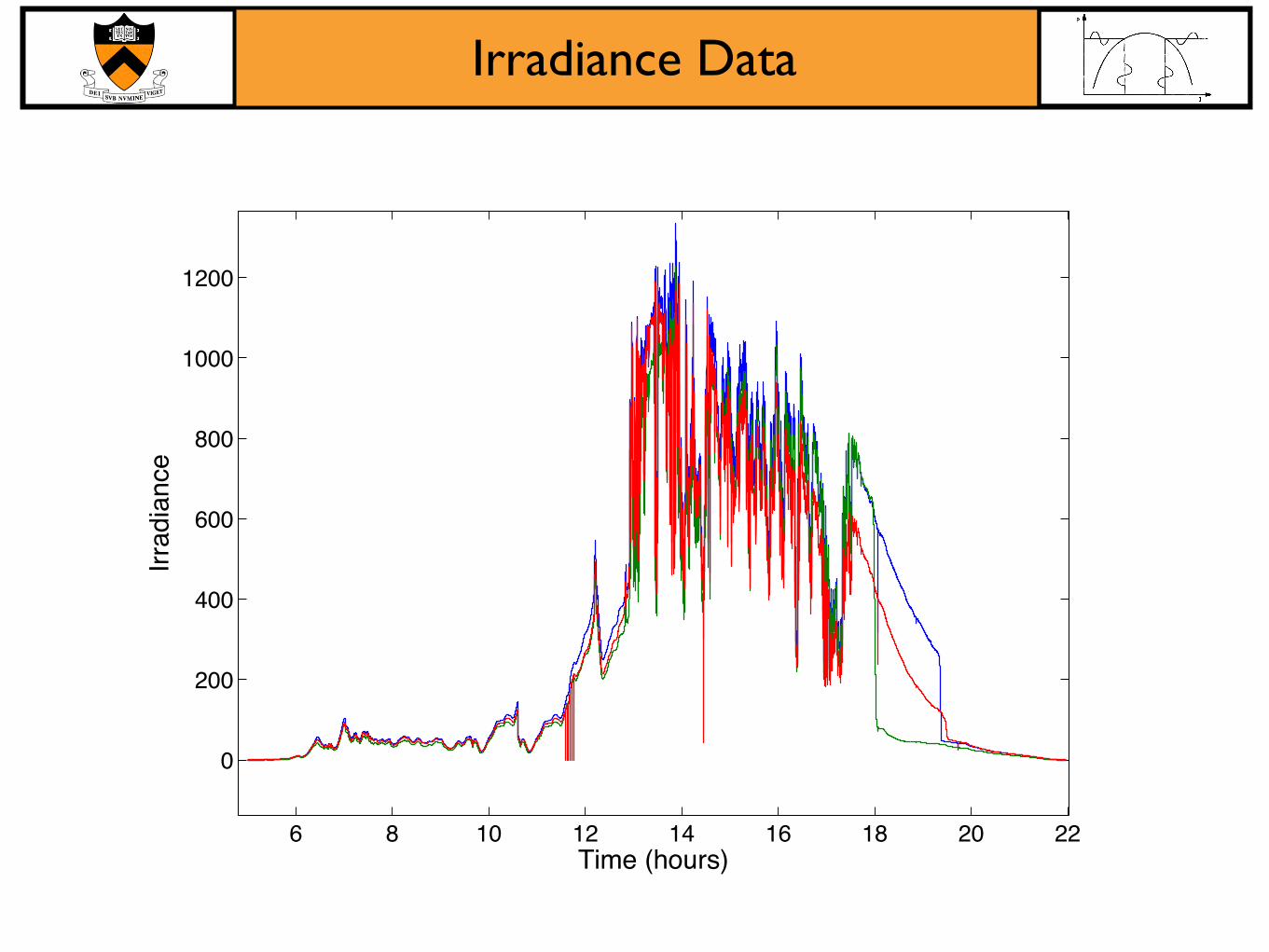
Irradiance Data

6 8 10 12 14 16 18 20 22

0

200

400

600

800

1000

1200

Time (hours)

Irra

dia

nce

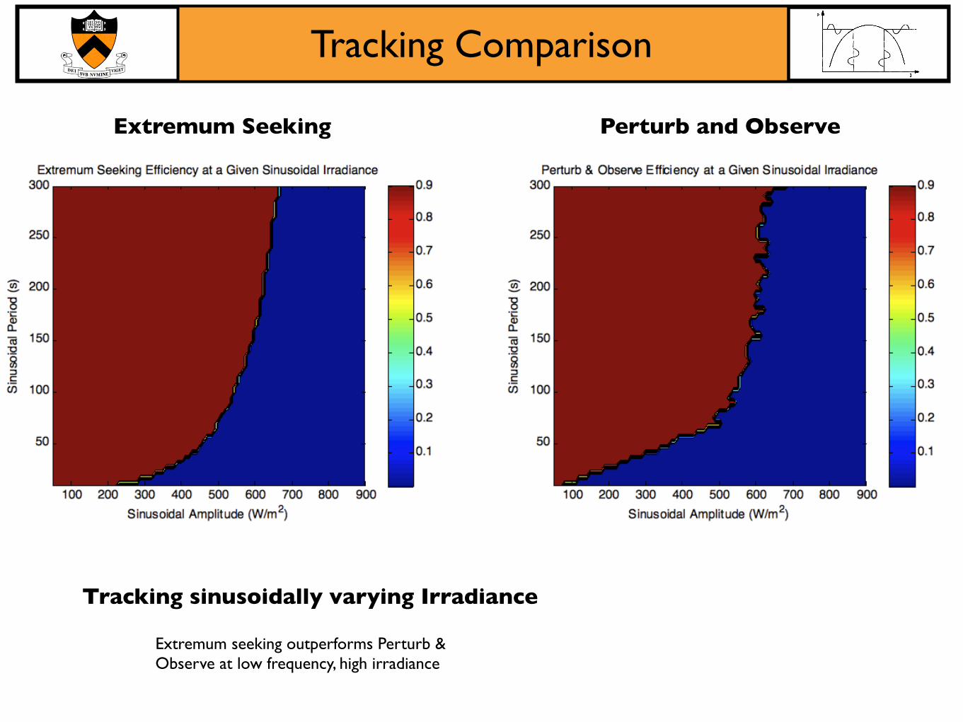
Tracking Comparison

Extremum seeking outperforms Perturb & Observe at low frequency, high irradiance

Tracking sinusoidally varying Irradiance

Extremum Seeking Perturb and Observe

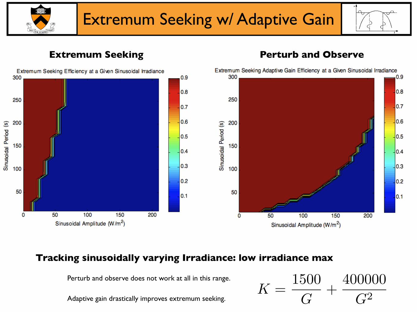
Extremum Seeking w/ Adaptive Gain

Extremum Seeking Perturb and Observe

Perturb and observe does not work at all in this range.

Tracking sinusoidally varying Irradiance: low irradiance max

Adaptive gain drastically improves extremum seeking.K =

1500G

+400000

G2