Embed Size (px)
Citation preview
Protocol Parameter Optimization and Characterization of
Superconducting Nanowire Single Photon Detector
by
He Xu
A thesis submitted in conformity with the requirementsfor the degree of Master of Applied Science
Graduate Department of Electrical and Computer EngineeringUniversity of Toronto
Copyright c© 2014 by He Xu
Abstract
Protocol Parameter Optimization and Characterization of
Superconducting Nanowire Single Photon Detector
He Xu
Master of Applied Science
Graduate Department of Electrical and Computer Engineering
University of Toronto
2014
The unconditional security of QKD is based on quantum physics. However, uncon-
ditional security, which relies on reasonable assumptions, is not the same as absolute
security, which make no assumptions, and QC protocols can be breached by means of
side channels. Recently, Measurement Device Independent QKD (MDI-QKD) has been
proposed to remove the side channels.
In parallel to improving performance by optimization, superconducting Nanowire Sin-
gle Photon Detector (SNSPD) has emerged among others as a promising technology. In
this thesis, we present a characterization procedure of SNSPD, and we report the impor-
tant finding of the phenomenon of afterpulse”, which is a clustered detection event at
180ns after a first event in a chain. Then, we postulate that the origin of this afterpulse
is from the limited bandwidth of the amplifier. By replacing the amplifiers with those
with a larger bandwidth, the phenomenon of afterpulse disappears.
ii

Acknowledgements
First, I thanks my supervisor Professor Hoi-Kwong Lo, who guided me and provided
me with the resources enabling the publication of this thesis. Over the years of my
M.A.Sc degree, his continuing support has transformed me from a mediocre student to
an into-the-field person.
The second token of thank goes to a collection of my prestige colleagues: Viacheslav
Burenkov, Feihu Xu and Zhiyuan Tang. The have offered support in a number of facets
to my thesis.
Next, I would like to thank my old committee members, Professor Joyce Poon and
Professor Lacra Pavel and a new committee member, Professor Amr S. Helmy. From the
beginning of my proposal to the end of my thesis, their spiritual help to me has been a
indisposable support to aid me going forward.
Last but not least, I would like to thank my family and all those who helped me getting
through. I have left out many individuals who supported me, but I greatly appreciate
their assistance.
iii
Contents
1 Introduction 1
1.1 Motivation . . . . . . . . . . . . . . . . . . . . . . . . . . . . . . . . . . . 1
1.2 Quantum Key Distribution in General . . . . . . . . . . . . . . . . . . . 2
1.3 Measurement Device Independent QKD . . . . . . . . . . . . . . . . . . . 2
1.4 Protocol Optimization . . . . . . . . . . . . . . . . . . . . . . . . . . . . 4
1.5 SSPD as a Better Device . . . . . . . . . . . . . . . . . . . . . . . . . . . 4
1.6 Significance and Outline . . . . . . . . . . . . . . . . . . . . . . . . . . . 5
1.7 Publications Related to This Work . . . . . . . . . . . . . . . . . . . . . 6
2 Basics of Quantum Key Distribution (QKD) 8
2.1 BB84 Protocol . . . . . . . . . . . . . . . . . . . . . . . . . . . . . . . . 8
2.2 Decoy States . . . . . . . . . . . . . . . . . . . . . . . . . . . . . . . . . . 10
2.3 Decoy State MDI-QKD . . . . . . . . . . . . . . . . . . . . . . . . . . . . 13
2.4 Convex Optimization . . . . . . . . . . . . . . . . . . . . . . . . . . . . . 15
2.4.1 Exhaustive Search . . . . . . . . . . . . . . . . . . . . . . . . . . 16
2.4.2 Local Search . . . . . . . . . . . . . . . . . . . . . . . . . . . . . . 17
2.5 Superconducting Nanowire Single Photon Detector . . . . . . . . . . . . 19
2.5.1 Detection Efficiency . . . . . . . . . . . . . . . . . . . . . . . . . . 19
2.5.2 Dark Count Rate . . . . . . . . . . . . . . . . . . . . . . . . . . . 19
2.5.3 Dead Time . . . . . . . . . . . . . . . . . . . . . . . . . . . . . . 20
2.5.4 Timing Jitter . . . . . . . . . . . . . . . . . . . . . . . . . . . . . 20
2.5.5 Afterpulsing . . . . . . . . . . . . . . . . . . . . . . . . . . . . . . 20
2.5.6 Number Resolving Detector VS. Threshold Detector . . . . . . . . 21
3 Protocol Parameter Optimization 22
3.1 Convex Topology . . . . . . . . . . . . . . . . . . . . . . . . . . . . . . . 23
3.2 Computational Resource . . . . . . . . . . . . . . . . . . . . . . . . . . . 23
iv
3.3 Key Rate Comparison between Optimization and Non-optimization . . . 24
3.4 Practical Choices of Optimization . . . . . . . . . . . . . . . . . . . . . . 27
3.5 Choosing the Number of Decoy . . . . . . . . . . . . . . . . . . . . . . . 29
3.6 Effect of the smallest decoy state ω . . . . . . . . . . . . . . . . . . . . . 30
3.7 Asymmetric MDI-QKD . . . . . . . . . . . . . . . . . . . . . . . . . . . . 32
3.8 Summary . . . . . . . . . . . . . . . . . . . . . . . . . . . . . . . . . . . 34
3.9 Conclusion . . . . . . . . . . . . . . . . . . . . . . . . . . . . . . . . . . . 35
4 Characterization of Single Photon Superconducting Detector 36
4.1 Introduction . . . . . . . . . . . . . . . . . . . . . . . . . . . . . . . . . . 36
4.2 Physics of SNSPD . . . . . . . . . . . . . . . . . . . . . . . . . . . . . . . 39
4.3 Experimental set-up of SNSPD . . . . . . . . . . . . . . . . . . . . . . . 39
4.4 Afterpulsing of Dark Counts . . . . . . . . . . . . . . . . . . . . . . . . . 42
4.5 Model for afterpulsing . . . . . . . . . . . . . . . . . . . . . . . . . . . . 46
4.6 Afterpulsing with laser on . . . . . . . . . . . . . . . . . . . . . . . . . . 48
4.7 Detection efficiency recovery . . . . . . . . . . . . . . . . . . . . . . . . . 49
4.8 Using an amplifier with improved low frequency response . . . . . . . . . 51
4.9 Summary and Conclusions . . . . . . . . . . . . . . . . . . . . . . . . . . 52
5 Conclusion and outlook 54
5.1 Conclusion: . . . . . . . . . . . . . . . . . . . . . . . . . . . . . . . . . . 54
5.1.1 Protocol Optimization: . . . . . . . . . . . . . . . . . . . . . . . . 54
5.1.2 Detector Characterization: . . . . . . . . . . . . . . . . . . . . . . 55
5.1.3 General Conclusion: . . . . . . . . . . . . . . . . . . . . . . . . . 55
A Numerical approaches 56
B Analytical approaches 58
B.0.4 One decoy state . . . . . . . . . . . . . . . . . . . . . . . . . . . . 58
B.0.5 Two decoy states . . . . . . . . . . . . . . . . . . . . . . . . . . . 59
C Simulation in Simulink 60
Bibliography 62
v
List of Tables
2.1 BB84 protocol Demonstration of the BB84 at each of the stages. Bit
Sequence are classical information encoded onto the rectilinear or diag-
onal basis of the polarizatoin qubits. the sifted data are again classical
information resulting from classical postprocessing of raw data . . . . . . 12
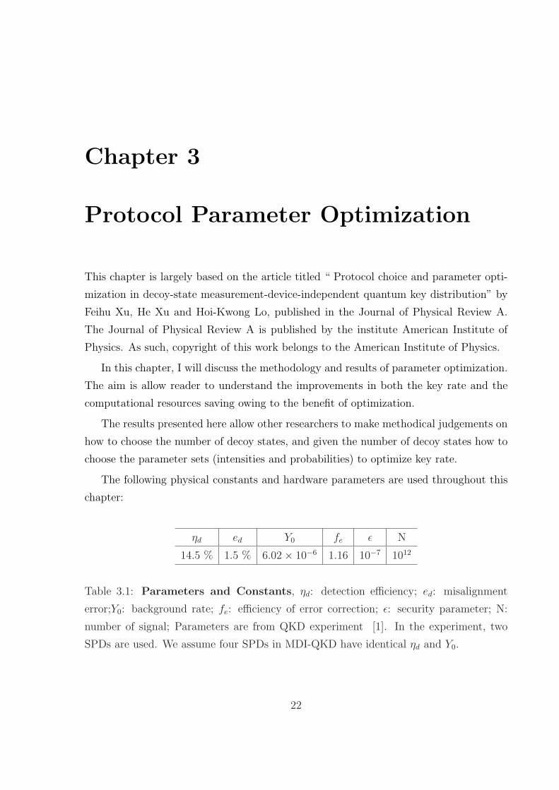
3.1 Parameters and Constants, ηd: detection efficiency; ed: misalignment
error;Y0: background rate; fe: efficiency of error correction; ε: security
parameter; N: number of signal; Parameters are from QKD experiment
[1]. In the experiment, two SPDs are used. We assume four SPDs in
MDI-QKD have identical ηd and Y0. . . . . . . . . . . . . . . . . . . . . . 22
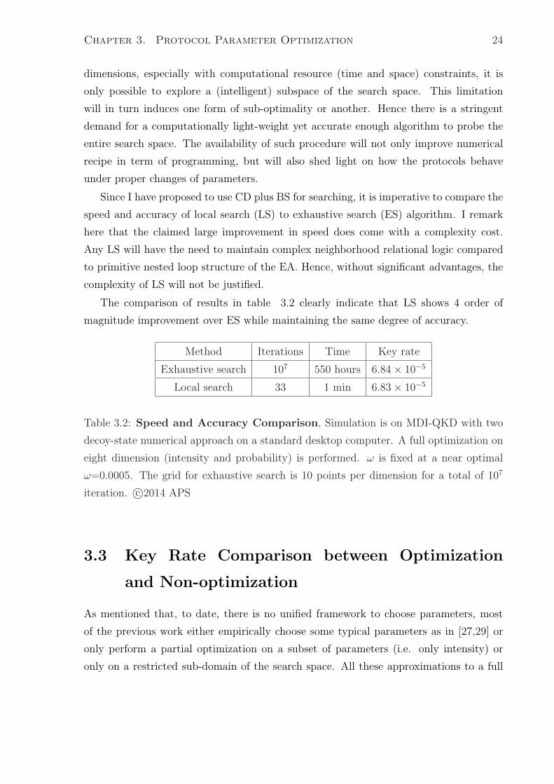
3.2 Speed and Accuracy Comparison, Simulation is on MDI-QKD with
two decoy-state numerical approach on a standard desktop computer. A
full optimization on eight dimension (intensity and probability) is per-
formed. ω is fixed at a near optimal ω=0.0005. The grid for exhaustive
search is 10 points per dimension for a total of 107 iteration. c©2014 APS 24
3.3 Comparison of parameters at 50km standard fiber. More general com-
parison results are shown in Fig. 3.3. The 2nd column is the optimal
parameters after a full parameter optimization. The 3rd and 4th columns
are respectively the parameters from Refs. [2] and [3]. We can see that full
optimization can improve the key rate R over one order of magnitude over
the non-full-optimization of Refs. [2, 3]. This improvement mainly comes
from optimizing the choices of intensities and probabilities. Notice that for
the smallest decoy-state ω, modulating the optimal value of around 10−6
is usually difficult in decoy-state QKD experiments [4, 5, 6, 7]. However,
we find that as long as the intensity of ω is below 1 × 10⁻³, the key rate
is very close to the optimum. c©2014 APS . . . . . . . . . . . . . . . . . 26
vi

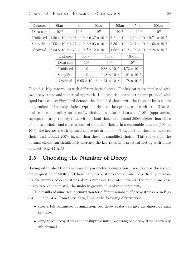
3.4 Key rate values with different basis choices. The key rates are simulated
with two decoy states and numerical approach. Unbiased denotes the
standard protocol with equal basis choice; Simplified denotes the simpli-
fied choice with the (biased) basis choice independent of intensity choice;
Optimal denotes the optimal choice with the (biased) basis choice depend-
ing on intensity choice. In a large data-set of 1018 (approaching asymptotic
case), the key rates with optimal choice are around 300% higher than those
of unbiased choice and close to those of simplified choice. In a reasonable
data-set (1012 to 1014), the key rates with optimal choice are around 300%
higher than those of unbiased choice and around 200% higher than those
of simplified choice. This shows that the optimal choice can significantly
increase the key rates in a practical setting with finite data-set. c©2014 APS 29
3.5 Optimal key values under different number of decoy states. With finite
data-set, the key rates with two decoy states are around one order of mag-
nitude higher than the ones with one decoy state. Three decoy states
cannot help to improve the key rates. Hence, two decoy states can achieve
a near optimal key rate. In the case of two decoy states, the numerical
method (Num) can only improve the key around 2% over the ones using
our analytical method (Ana). This shows that the two decoy-state ana-
lytical method presented in Appendix B can also result in a near optimal
estimation. c©2014 APS . . . . . . . . . . . . . . . . . . . . . . . . . . . 32
vii

List of Figures
2.1 setup of BB84 Protocol [8] Source: single -photon source; RNG:
random number generator; PC: polarization controller;PBS: polarization
beam splitter; D0/D1: single-photon detectors,from published thesis [8] 8
2.2 Flow of BB84 Protocol Alice and Bob each produce a randomly gen-
erated basis sequence, and a randomly generated/measured bit sequence.
after sifting, they share a common bitstream . . . . . . . . . . . . . . . . 9
2.3 Setup of MDI-QKD Protocol WCP: weak coherent pulse; Pol-M: po-
larization modulator; Decoy-IM: intensity modulator; BS: beam splitter;
PBS: polarizing beam splitter; Dx: photo detectors c©2012 Physical Re-
view letters . . . . . . . . . . . . . . . . . . . . . . . . . . . . . . . . . . 13
2.4 Error Contour e1,e2: one of the dimensions of the optimization. All
points on the same ellipse have the same error, where the error of a point
is quantified by how far (in euclidian distance) the point is from the the-
oretical optimal point. The larger the radius of the ellipse, the larger the
error, (again) quantified by the euclidean distance away from the optimal-
ity, the dot represent 0 error or optimality. . . . . . . . . . . . . . . . . 16
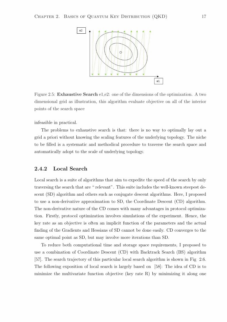
2.5 Exhaustive Search e1,e2: one of the dimensions of the optimization. A
two dimensional grid as illustration, this algorithm evaluate objective on
all of the interior points of the search space . . . . . . . . . . . . . . . . 17
2.6 Local Search e1,e2: basis of optimization. A two dimensional descent
sequence. The error contour structure allow the optimization to evaluate
only a small subset of the search space. Here we shown that this subset
lies on the descent path of the algorithm. c©2014 APS . . . . . . . . . . . 18
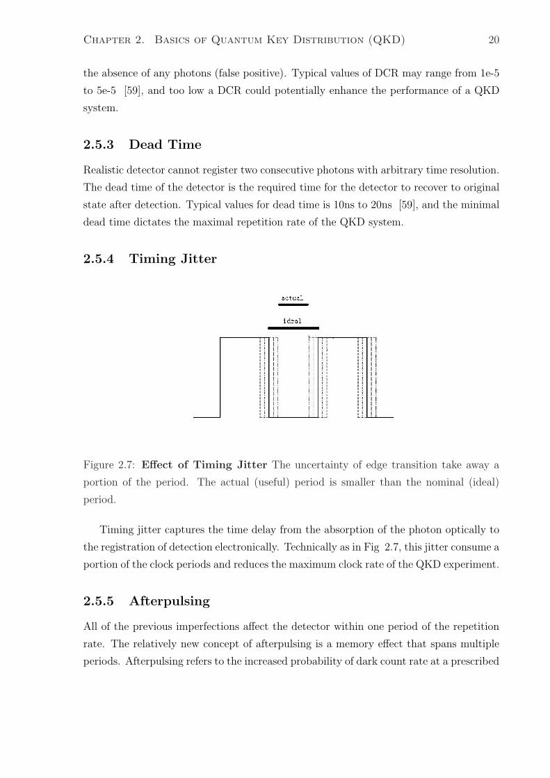
2.7 Effect of Timing Jitter The uncertainty of edge transition take away
a portion of the period. The actual (useful) period is smaller than the
nominal (ideal) period. . . . . . . . . . . . . . . . . . . . . . . . . . . . 20
viii
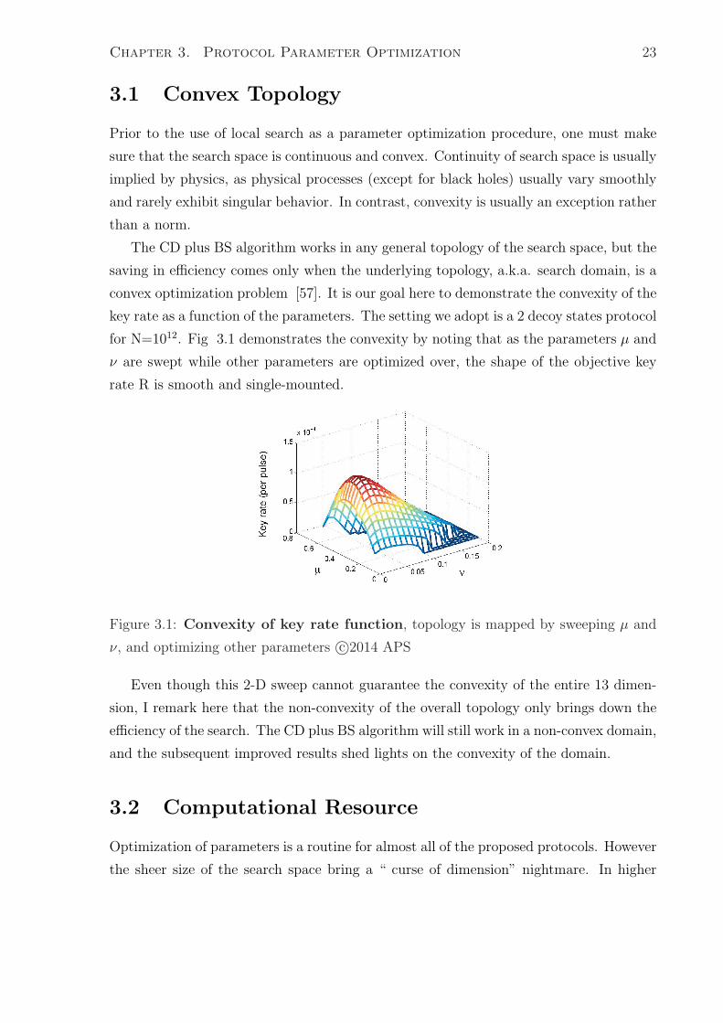
3.1 Convexity of key rate function, topology is mapped by sweeping µ
and ν, and optimizing other parameters c©2014 APS . . . . . . . . . . . 23
3.2 Key rate comparison with infinite data-set. The dotted black curve
is the perfect key rate with infinite decoy states. The blue solid curve
is our optimized key rate using the numerical approach with two decoy
states, where the intensities are ω=0.0005, ν=0.01 and optimized µ. For
comparison purpose, we present the non-optimized and partially-optimized
key rates using the methods and parameters of Refs [2, 3, 9]: the black
dashed curve is using [3] with ω=0, ν=0.01 and optimized µ; the red
dashed curve is using [9] with ω=0.01, ν=0.1 and µ=0.3; the green dashed
curve is using [2] with ω=0, ν=0.1 and µ=0.5. Notice that if the parameter
optimization is also applied to Refs [2, 9], all the key rates are almost the
same. In the asymptotic case, parameter optimization is simple, as only
the intensities are required to be optimized and a smaller value of decoy-
state intensity can in principle result in a better estimation. Parameter
optimization can still increase the key rate and extend the secure distance.
c©2014 APS . . . . . . . . . . . . . . . . . . . . . . . . . . . . . . . . . . 25
3.3 Practical key rate comparison (with statistical fluctuations). The
optimal parameters and key rate in the distance of 50km (standard fiber)
are shown in Table 3.3. All the key rates are simulated with N=1012. The
blue solid and red dashed-dotted curves (almost overlapped) are respec-
tively our optimized key rates (after a full optimization) using the numer-
ical (Appendix A) and analytical (Appendix B) methods with two decoy
states. The black dashed curve is using the method of Ref. [3], where only
partial parameters (ie, the intensities) are optimized. The green dashed
curve is using the method of Ref. [2], where some typical parameters are
assumed without optimization. Without full parameter optimization, the
key rates in Refs [2, 3] are around one order of magnitude lower than
ours across different distances. Our method can enable secure MDI-QKD
over 25km longer than [2, 3]. These results highlight the importance of
parameter optimization in practical decoy-state MDI-QKD. c©2014 APS 27
ix
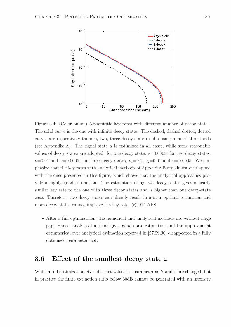
3.4 (Color online) Asymptotic key rates with different number of decoy states.
The solid curve is the one with infinite decoy states. The dashed, dashed-
dotted, dotted curves are respectively the one, two, three decoy-state re-
sults using numerical methods (see Appendix A). The signal state µ is
optimized in all cases, while some reasonable values of decoy states are
adopted: for one decoy state, ν=0.0005; for two decoy states, ν=0.01 and
ω=0.0005; for three decoy states, ν1=0.1, ν2=0.01 and ω=0.0005. We
emphasize that the key rates with analytical methods of Appendix B are
almost overlapped with the ones presented in this figure, which shows that
the analytical approaches provide a highly good estimation. The estima-
tion using two decoy states gives a nearly similar key rate to the one with
three decoy states and is higher than one decoy-state case. Therefore,
two decoy states can already result in a near optimal estimation and more
decoy states cannot improve the key rate. c©2014 APS . . . . . . . . . . 30
3.5 (Color online) Secret key rate in logarithmic scale as a function of the
distance under different numbe of decoy states. The main figure is for
data-set N=1012 and the inserted figure is for N=1014. The key rates
are obtained using numerical methods with one (dashed curve), two (solid
curve), three (dashed-dotted curve) decoy states. The key rates with two
and three decoy states are almost overlapped. In simulation, we perform a
full parameter optimization for all cases. Our results show that after a full
parameter optimization, the two decoy-state method can give an almost
optimal key rate, which is higher than the one with one decoy state. Three
decoy states cannot help to increase the key rate. c©2014 APS . . . . . . . 31
3.6 (b) Key rate as a function of the decoy state ω. As long as the intensity of
ω is below 1× 10⁻³, the key rate is very close to the optimum. A perfect
vaccum (ω = 0) is not essentially required in practical decoy-state QKD
experiments. c©2014 APS . . . . . . . . . . . . . . . . . . . . . . . . . . 33
3.7 comparison of the 3 choice of parameter: simplified, symmetric
and fully-optimized the simplified choice results in identical 0 key rate.
the symmetric case is close to the fully-optimized result but should be the
one adopted in practice. c©2014 APS . . . . . . . . . . . . . . . . . . . . 33
x
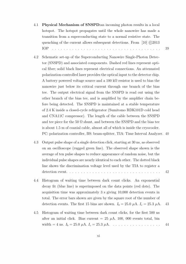
4.1 Physical Mechanism of SNSPD:an incoming photon results in a local
hotspot. The hotspot propagates until the whole nanowire has made a
transition from a superconducting state to a normal resistive state. The
quenching of the current allows subsequent detections. From [10] c©2013
IOP . . . . . . . . . . . . . . . . . . . . . . . . . . . . . . . . . . . . . . 39
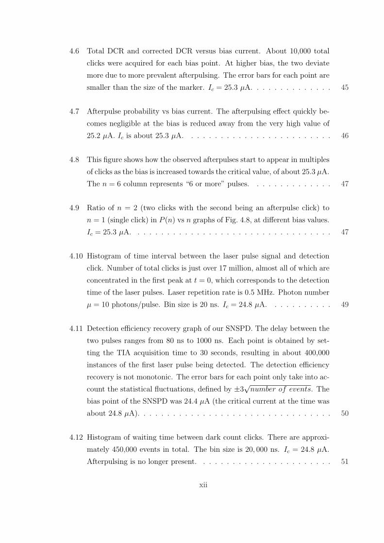
4.2 Schematic set-up of the Superconducting Nanowire Single-Photon Detec-
tor (SNSPD) and associated components. Dashed red lines represent opti-
cal fiber; solid black lines represent electrical connections. An attenuated
polarization-controlled laser provides the optical input to the detector chip.
A battery powered voltage source and a 100 kΩ resistor is used to bias the
nanowire just below its critical current through one branch of the bias
tee. The output electrical signal from the SNSPD is read out using the
other branch of the bias tee, and is amplified by the amplifier chain be-
fore being detected. The SNSPD is maintained at a stable temperature
of 2.4 K inside a closed-cycle refrigerator (Sumitomo RDK101D cold head
and CNA11C compressor). The length of the cable between the SNSPD
and tee piece for the 50 Ω shunt, and between the SNSPD and the bias tee
is about 1.5 m of coaxial cable, almost all of which is inside the cryocooler.
PC: polarization controller, BS: beam-splitter, TIA: Time Interval Analyzer. 40
4.3 Output pulse shape of a single detection click, starting at 30 ns, as observed
on an oscilloscope (rugged green line). The observed shape shown is the
average of ten pulse shapes to reduce appearance of random noise, but the
individual pulse shapes are nearly identical to each other. The dotted black
line shows the discrimination voltage level used by the TIA to register a
detection event. . . . . . . . . . . . . . . . . . . . . . . . . . . . . . . . . 42
4.4 Histogram of waiting time between dark count clicks. An exponential
decay fit (blue line) is superimposed on the data points (red dots). The
acquisition time was approximately 3 s giving 10,000 detection events in
total. The error bars shown are given by the square root of the number of
detection events. The first 15 bins are shown. Ib = 25.0 µA. Ic = 25.3 µA. 43
4.5 Histogram of waiting time between dark count clicks, for the first 500 ns
after an initial click. Bias current = 25 µA. 100, 000 events total, bin
width = 4 ns. Ib = 25.0 µA. Ic = 25.3 µA. . . . . . . . . . . . . . . . . . 44
xi
4.6 Total DCR and corrected DCR versus bias current. About 10,000 total
clicks were acquired for each bias point. At higher bias, the two deviate
more due to more prevalent afterpulsing. The error bars for each point are
smaller than the size of the marker. Ic = 25.3 µA. . . . . . . . . . . . . . 45
4.7 Afterpulse probability vs bias current. The afterpulsing effect quickly be-
comes negligible at the bias is reduced away from the very high value of
25.2 µA. Ic is about 25.3 µA. . . . . . . . . . . . . . . . . . . . . . . . . 46
4.8 This figure shows how the observed afterpulses start to appear in multiples
of clicks as the bias is increased towards the critical value, of about 25.3 µA.
The n = 6 column represents “6 or more” pulses. . . . . . . . . . . . . . 47
4.9 Ratio of n = 2 (two clicks with the second being an afterpulse click) to
n = 1 (single click) in P (n) vs n graphs of Fig. 4.8, at different bias values.
Ic = 25.3 µA. . . . . . . . . . . . . . . . . . . . . . . . . . . . . . . . . . 47
4.10 Histogram of time interval between the laser pulse signal and detection
click. Number of total clicks is just over 17 million, almost all of which are
concentrated in the first peak at t = 0, which corresponds to the detection
time of the laser pulses. Laser repetition rate is 0.5 MHz. Photon number
µ = 10 photons/pulse. Bin size is 20 ns. Ic = 24.8 µA. . . . . . . . . . . 49
4.11 Detection efficiency recovery graph of our SNSPD. The delay between the
two pulses ranges from 80 ns to 1000 ns. Each point is obtained by set-
ting the TIA acquisition time to 30 seconds, resulting in about 400,000
instances of the first laser pulse being detected. The detection efficiency
recovery is not monotonic. The error bars for each point only take into ac-
count the statistical fluctuations, defined by ±3√
number of events. The
bias point of the SNSPD was 24.4 µA (the critical current at the time was
about 24.8 µA). . . . . . . . . . . . . . . . . . . . . . . . . . . . . . . . . 50
4.12 Histogram of waiting time between dark count clicks. There are approxi-
mately 450,000 events in total. The bin size is 20, 000 ns. Ic = 24.8 µA.
Afterpulsing is no longer present. . . . . . . . . . . . . . . . . . . . . . . 51
xii

C.1 Simulink Model The model paritions into 3 main sections: Source, cir-
cuit and Read-out parts. 1) source section models the incoming photon
as a nonlinear transition of SSPD. 2) circuit section models the normal
state as a resistor and superconducting state as a non-dissipative wire.
3) read-out parts models the radio-frequency (RF) amplifier and filter by
gain and transfer functions . . . . . . . . . . . . . . . . . . . . . . . . . . 61
xiii
Chapter 1
Introduction
1.1 Motivation
The twenty-first century is an era of information, and the exponential growth in the
generation of data by the Internet and the World Wide Web (WWW) can lead to in-
formation black holes in organizations servers and even in home computers. Such an
astonishing amount of information must be stored electronically for ease of manipulation
and distribution. As a by-product of the use of electronic information, the concept of
cyber-security has become a recurring issue.
Ever since the invention of the Caesar cipher it spurred an arm race between commu-
nicating parties and potential adversaries. The simplicity of using substitution schemes
as ciphers is only capable of foiling the most simple-minded adversaries. The advent of
the Ron Rivest, Adi Shamir and Leonard Adleman (RSA) algorithm [11] brought us
computational security as opposed to unconditional security. The security of the RSA
is based on the presumed difficulty of factoring a large product of two primes efficiently.
Hence, the approach of computational security only shifted the arm race from a search
for algorithms to a search for computational power.
Shannon’s proof of information theoretic security created the interest in the scheme
of One Time Pad (OTP) [12]. The OTP is impossible to crack and provides information
theoretical security as proved by C. Shannon [13]. While conceptually pleasing, the OTP
is not practical because it requires a key as long as the message. This need of distributing
the long key can be as difficult as distributing a message itself. Then, the open question
is: Can this snowballing arm race be ended?
In contrast to all its predecessors, quantum cryptography holds the promise of un-
1
Chapter 1. Introduction 2
conditional security [14, 15, 16]. However, at the time of writing, the technology of
quantum cryptography is still at its infancy, much inter-disciplinary work would have to
be done to bring quantum cryptography to commercial products. However, Quantum
Key distribution (QKD) protocols, among many other quantum cryptographic protocols,
can be implemented with the components of current technology. Coincidentally, the
requirements for distributing the long key from the OTP can be done via QKD [17, 18,
19]. The distribution of keys as long as the message with QKD followed by the OTP is
the right combination that leverages the state-of-the-art of both classical and quantum
communication technologies.
1.2 Quantum Key Distribution in General
Quantum cryptography was born when Stephen Wiesner proposed around 1970 the idea
of quantum money that cannot be counterfeited. Stephen Wiesner’s paper remained un-
published for more than a decade [17]. In 1984, Bennett and Brassard invented quantum
key distribution (QKD), the most well-known application of quantum cryptography [18].
Their protocol BB84 remains the best-known protocol for QKD.
At the heart of the BB84 is its encoding of information on quantum states, such as
polarization of a photon or spin of an electron. By virtue of the famous “quantum no-
cloning” theorem and its related consequences, “information gain implies disturbance”
[20, 21], the BB84 guarantees that: by encoding the information on one of many quantum
states from a set of distinct non-orthogonal states, no information can be leaked without
disturbing the states. While a potential adversary can still do evesdropping on the states,
she must reveal herself to the communication parties. As will be seen later, this revelation
is manifested in a increased Bit Error Rate (BER) at the receiver.
QKD, among other quantum cryptography protocols, is the most technological feasi-
ble protocols. Much to be expected, QKD networks have been successfully deployed in
Africa [22], China [23] and Tokyo [24].
1.3 Measurement Device Independent QKD
The BB84 and its relatives provide theoretical unconditional security, but there is a large
gap between theory and practice. In practice, the adversaries’ attack is not usually on the
protocol itself, but rather on the implementation technologies such as sources, detectors
Chapter 1. Introduction 3
and modulators.
On the source side, a true Single Photon Source (SPS) is completely missing, and
the laboratory practice is to use a heavily attenuated classical coherent source such
that the probability of emitting two or more photons is small. The finite probability
of emission of two or more photons gives rise to a well-known photon-number-splitting
(PNS) attack [25, 26]. For example, when it is possible to split a classical pulse, the
adversary will have as much information as the receiver; rendering the quantum protocol
useless. Fortunately, the PNS can be foiled by phase-randomization [27] and decoy states
[28, 29, 30] techniques.
Also, on the modulator and detector sides, practical implementations are rarely with-
out jitters and dead time. Jitters, also known as the uncertainty of the pulse arrival
time, provide timing information on when the detectors are likely to mix the current and
the next bit in the bit stream. Dead time, also known as the inability of detector to
recover instantaneously, provides timing information on when the detectors are likely to
have low detection efficiency. Moreover, practical detectors can only tell the absence or
presence of a photon stream, but cannot tell the exact number of photons in the stream.
It has been shown that these “ timing cues” or loopholes can leak significant amount of
information to evesdroppers, and the time-shift attack [31, 32], the blinding attack [33]
and the phase-remapping attack [34] have exploited it. Therefore, a big question in the
quantum cryptography is the following: are practical QKD systems really secure?
To close the gap, there is a strong desire to have a loophole-free QKD protocol. The
proposed device-independent (DI-QKD) [35] closes all these loopholes [31, 32, 34], but it
places strong requirements on the implementation technologies; for example, the required
near-unity detection efficiency is not practical. Furthermore, the extremely low rate at
practical distance [36] also refrains the users’ from adopt the protocol. Are side channels
unavoidable?
The Measurement-Device-Independent QKD (MDI-QKD) [37] answers this question
negatively. This principle that underlies MDI-QKD is the fact that most of the attacks
are on the detector side, or most of the loopholes can be closed with perfect measurement
devices. At the same time, the more stringent requirement of MDI on state preparation
[38] (or source) can be done with current state-of-the-art technology. Incidentally, many
recent experiments on MDI-QKD [39, 40, 41, 42, 43, 44] have demonstrated the realiz-
ability of MDI-QKD.
Chapter 1. Introduction 4
1.4 Protocol Optimization
The protocols of MDI-QKD only dictate the operation of the communication, but there
is no prescription for how the parameters are chosen [16, 37]. Well chosen parameters set
for a protocol can result in a much shorter run-time and much simpler implementation
[45, 3, 46, 2]. On the other hand, an MDI-QKD experiment with a bad parameter set can
result in so low a key rate that efforts are wasted in to improve resolution of electronic
and optical equipments.
The importance of parameters optimization of protocols cannot be over-emphasized.
It is the aim of this thesis to provide a systematic framework for the optimization of
parameters. The end results of the optimization procedure are values of parameters that
can be implemented in devices controlling the operation of the protocol.
1.5 SSPD as a Better Device
The imperfections of detectors such as jitter and dead time cannot be eliminated com-
pletely, but it is possible to improve the detectors and minimize the impacts of these
imperfections.
Solid-state Single-Photon Avalanche Diode (SPAD) is able to detect single photons
in reverse-biased mode [47]. An incoming photon creates electron-hole pair by impact
ionization [48]. This process continues and manifests itself as a macroscopic current,
which is able to be picked up by a conventional detector.
Superconducting Nanowire Single Photon Device (SNSPD) is an emerging technology
that offers superior performance than SPAD, for example: a shorter dead time and low
jitter [49]. However, such technology has yet to be understood completely in terms of
its responses to single photon and/or multi-photons excitations. However, it is known
that SNSPD consists of a nanowire of superconducting material. A single photon hits
the detector and creates a propagating hotspot until the whole segment is no longer
superconducting. The resulting voltage pulse generated from the transition is detected
after amplification, and subsequent detection is enabled by active quenching.
The characterization of SNSPD cannot be done in isolation from other parts of the
system. Realistically, the SNSPD will likely be enclosed in a DC Biasing network and
an RF readout network (detailed later in chapter 4). It is the finding of this thesis that
the imperfections of these peripheral circuitries can be even more detrimental than the
imperfections of the SNSPD device itself.
Chapter 1. Introduction 5
1.6 Significance and Outline
The aim of the thesis is to provide some guidelines in characterization of SNSPD and in
parameter optimization of MDI-QKD. The recurring themes are the improvement and
characterization of performance of device and/or protocol by optimizing the influential
parameters. To accomplish this exposition, the remaining thesis is organized as follows:
• Chapter 2 lays the foundations for QKD and MDI-QKD for the rest of the thesis.
Main ingredients are :
– Sec 2.1 is a description of BB84 protocol
– Sec 2.2 introduction to the idea of “decoy state”
– Sec 2.3 description of MDI-QKD protocol
– Sec 2.4 introduction to Convex Optimization
– Sec 2.5 introduction to SNSPD
• Chapter 3 introduce the optimization procedure and its role in cryptography pro-
tocols. Chapter 3 also presents main results on parameter optimization and its
significance to practical implementations:
– Sec 3.1 explains convex topology and their advantages of optimization effi-
ciency.
– Sec 3.2 is a comparison of computational resources of different algorithms.
– Sec 3.3 highlights the key rate increase due to optimization
– Sec 3.4 suggests a way to choose the number of parameters in consideration
in the optimization
– Sec 3.5 recommends a guideline on the choice of protocol
– Sec 3.6 links to practice by explains how to do decoy when the practical
modulators cannot handle too small a modulation level.
– Sec 3.7 generalizes the work from a symmetric setup to a more realistic asym-
metric setup.
• Chapter 4 introduce SNSPD and its peculiarities, and also introduce main results
and characterization of SNSPD
Chapter 1. Introduction 6
– Sec 4.1 introduces the SNSPD as a novel device for Quantum Information (QI)
experiments
– Sec 4.2 explains our experiment setup and all equipments and devices involved
– Sec 4.3 introduces the phenomenon of AfterPulse and explains its statistical
distribution
– Sec 4.4 gives a model of afterpulse in experiments
– Sec 4.5 is on the experiment where afterpulse is not solely due to dark count,
but partly to dark count and the rest attributes to real detection events.
– Sec 4.6 confirms our hypothesis on the connection of afterpulse phenomenon
and the spurious increase of detection efficiency at recovery time
– Sec 4.7 provides an experimental method for elimination of the afterpulse
• Chapter 5 concludes the thesis and provide perspectives
Our works on protocol optimization and device characterization enables other QKD
researchers to better understanding of the origins and potentials of the protocol, e.g a
prescription on how the parameters are chosen. The results of our work presented here
allow other researchers to better cope with the non-idealities of practical device and the
underlying communication protocols. In particular, the 200 % increase in secure key rate
can significantly reduce the running time of the QKD experiments, or, conversely, can
boost the transmission distance given a fixed data acquisition time. Also, the claimed
superior performance of SNSPD can practical shift the burden of data post-processing
from digital software to the front-end detector; for example, the improvement in detection
efficiency can potentially compensate for the detrimental photon loss rate in fiber link,
and thus increase the transmission distance.
1.7 Publications Related to This Work
• Xu, Feihu, He Xu, and Hoi-Kwong Lo. “ Protocol choice and parameter optimiza-
tion in decoy-state measurement-device-independent quantum key distribution.”
Physical Review A 89.5 (2014): 052333. [50]
Details: 9 pages, double-column. Additional supplementary material online.
My contribution: I am the second author of the paper. I proposed to use the
Local Search Algorithm. I also performed most of the simulations and make-up

Chapter 1. Introduction 7
most of the pictures in the paper. Feihu Xu derived the analytical expressions
for simulation, and participated in writing of the paper. Hoi-Kwong Lo played a
supervisory role, and contributed trouble-shooting for the paper.
• Burenkov, Viacheslav, Xu, He, Bing Qi, Robert H. Hadfield, Hoi-Kwong LO “
Investigations of afterpulsing and detection efficiency recovery in superconduct-
ing nanowire single-photon detectors.” Journal of Applied Physics 113.21 (2013):
213102. [51]
Details: 11 pages, double-column.
My contribution: I am the second author of the paper. There are three major
parts of the project: 1) Afterpulse experiment, 2) Laser-on experiment and 3)
recovery curve experiment. Prior to my joining to the project, 1) is done. I have
participated in 2) mainly to help on the post-processing of data. I am directly
involved 3) in experimentation and in post-processing of the data. My roles in 2)
and 3) are focused on speeding-up the existing software and make the programming
more autonomous. Viacheslav Burenkov discovered the presence of the afterpulsing
effect, performed most of the experiments.Bing Qi assisted with some experiments
and contributed to trouble-shooting, discussions, and the writing of the paper.
Robert Hadfield provided insights regarding the detector, which was made in his
lab. Hoi-Kwong Lo played a supervisory role, and contributed to trouble-shooting,
discussions and the writing of the paper.

Chapter 2
Basics of Quantum Key Distribution
(QKD)
Quantum information Processing is an interdisciplinary field that brought together the
fields of Applied Mathematics, Physics, Computer Science and Engineering. The impact
of Quantum Information (QI) have been demonstrated in the Quantum Network devel-
oped in USA, Europe, China and Japan [22, 23, 24]. It is the aim of this chapter to
develop the background material for the subsequent progressions.
2.1 BB84 Protocol
The basic setup or model of the BB84 is in Fig 2.1, the setup indicates that the mod-
ulation format is polarization modulation. Hence, the stream of quantum carriers’ state
are made indistinguishable except for the polarization.
Figure 2.1: setup of BB84 Protocol [8] Source: single -photon source; RNG: random
number generator; PC: polarization controller;PBS: polarization beam splitter; D0/D1:
single-photon detectors,from published thesis [8]
8
Chapter 2. Basics of Quantum Key Distribution (QKD) 9
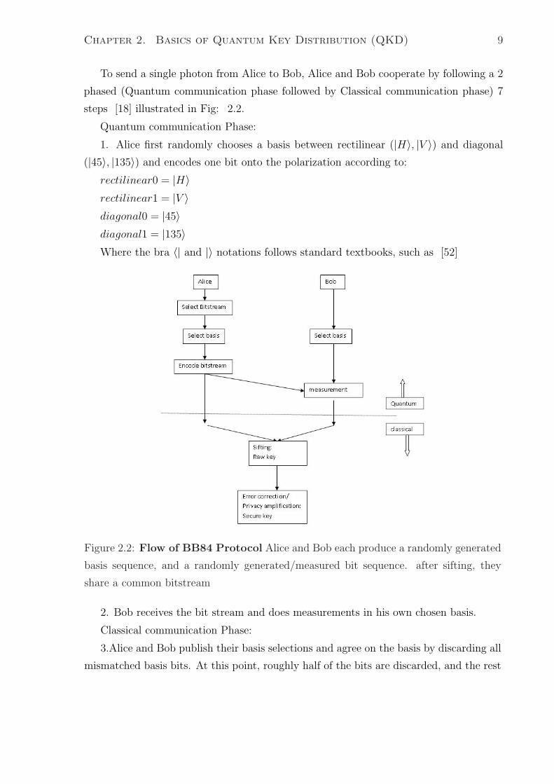
To send a single photon from Alice to Bob, Alice and Bob cooperate by following a 2
phased (Quantum communication phase followed by Classical communication phase) 7
steps [18] illustrated in Fig: 2.2.
Quantum communication Phase:
1. Alice first randomly chooses a basis between rectilinear (|H〉, |V 〉) and diagonal
(|45〉, |135〉) and encodes one bit onto the polarization according to:
rectilinear0 = |H〉rectilinear1 = |V 〉diagonal0 = |45〉diagonal1 = |135〉Where the bra 〈| and |〉 notations follows standard textbooks, such as [52]
Figure 2.2: Flow of BB84 Protocol Alice and Bob each produce a randomly generated
basis sequence, and a randomly generated/measured bit sequence. after sifting, they
share a common bitstream
2. Bob receives the bit stream and does measurements in his own chosen basis.
Classical communication Phase:
3.Alice and Bob publish their basis selections and agree on the basis by discarding all
mismatched basis bits. At this point, roughly half of the bits are discarded, and the rest
Chapter 2. Basics of Quantum Key Distribution (QKD) 10
are called raw keys.
4. Alice and Bob choose a fraction of remaining bits, and broadcast the bits’ positions
and polarizations. Then, Alice and Bob compute and compare the QBER of these bits.
If the QBER is larger than a (suitably chosen) threshold value, they abort the process.
5. if the QBER is acceptable, Alice and Bob then perform error correction and privacy
amplification to generate final secure keys.
Eve has no power to acquire the basis information of Alice and Bob. Hence, on aver-
age, she will have 50 percent chance of getting the right basis. Otherwise, for 50 percent
of the time, Eve will choose the wrong basis. So, this protocol can detect the presence
of Eve at the QBER computation and comparison phase by the following dichotomy:
1. If Eve chooses the correct basis, no error will be introduced by Eve.
2. If Eve chooses the wrong basis, the basis choice of Eves and Bob will be uncorre-
lated. Hence, Eve will introduce 50*50 =25 percent QBER in the comparison stage.
In conclusion, the 25 percent extra QERB cannot be hidden by Eve, and the BB84 can
reveal the presence of a passive evesdropper, which is a mission impossible for classical
information.
2.2 Decoy States
The BB84 protocol requires the source to be a truly single photon source. However, a
truly single photon source is still not realized with today’s technology. As a substitute,
heavily attenuated coherent sources, a.k.a. weak coherent state are used instead.
A weak coherent state is described by:
|α〉 = e−|a|22
∞∑n=0
αn
√n!|n〉 (2.1)
If the phase, θ, of alpha is uniformly randomized, i.e. θ = |α|Eiθ where θ is random,
then we get a density matrix of the following form:
ρA =1
2π
∫ 2π
0
∣∣|α|eiθ⟩⟨|α|eiθ
∣∣ (2.2)
=1
2π
∞∑n=0
∞∑m=0
|α|n+m
√n!m!
e−|α|2|n〉〈m|
∫ 2π
0
dθei(n−m)θ (2.3)
=∞∑
n=0
µn
n!e−µ|n〉〈n| (2.4)
Chapter 2. Basics of Quantum Key Distribution (QKD) 11
This density matrix contains not only single photon components, but also an arbitrary,
n, photon number states with a probability:
P (n) =µn
n!e−µ (2.5)
I remark here that, for the BB84 protocol, only single photon states can eventually
contribute to secure key rate, and the finite probability of multi-photon states opens up
to Eve the possibility of PNS attack. In this attack, Eve could keep all single photon
states in memory and split parts of multi-photon states to Bob to perform measurement
on kept parts of the multi-photon states. Only after Alice and Bob publicly announce
their basis, then will Eve perform measurements on single photon states to extract all of
the information.
The idea of decoy state is to overcome this limitation of weak coherent pulse by
introducing other sets of states besides the signal states. These extra decoy states have
average photon numbers ν 6= µ. The purposes of these extra states are not to generate
secure key rate, but only to reveal the presence of eavesdropping. In an actual key
distribution, the bit streams are encoded onto signal and decoy state randomly. Only
after Alice and Bob publicly announce their basis, Alice informs Bob the real indices of
his signal states. Since Eve has no way a-priori to distinguish the decoy to signal states,
his presence will be revealed via the increase of QBER.
To facilitate the subsequent discussion, the following definitions and relations are in
order:
• Pi,state probability, of i-photon state is the probability that exactly i photon are in
the coherent states. mathematically: Pi = µi
i!e−µ
• Yi, Yield, of i-photon state is the conditional probability of a detection event at
Bob given that Alice sent i photons.
• Qi, gain, of i-photon state is the probability that Alice’s i photons sent is registered
as detection at Bob.
• Qµ, overall gain, of a coherent pulse with mean photon µ is the probability that
the entire coherent state is registered as detection
• ei, QBER, of i-photon state is the probability that Alice’s i photons sent is err at
Bob
Chapter 2. Basics of Quantum Key Distribution (QKD) 12
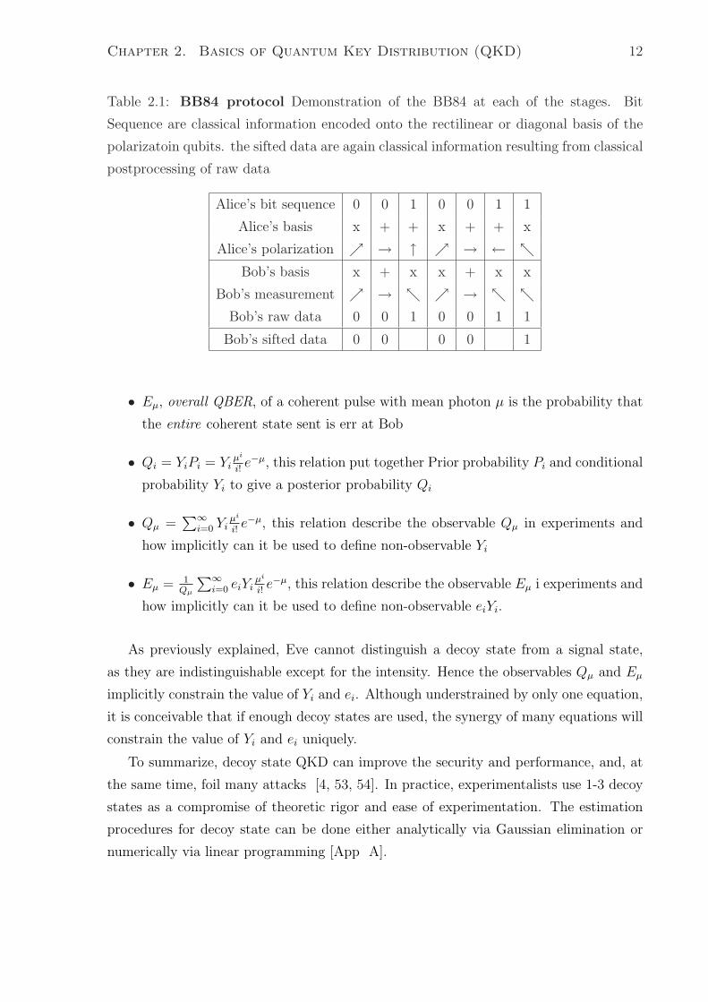
Table 2.1: BB84 protocol Demonstration of the BB84 at each of the stages. Bit
Sequence are classical information encoded onto the rectilinear or diagonal basis of the
polarizatoin qubits. the sifted data are again classical information resulting from classical
postprocessing of raw data
Alice’s bit sequence 0 0 1 0 0 1 1
Alice’s basis x + + x + + x
Alice’s polarization → ↑ → ← Bob’s basis x + x x + x x
Bob’s measurement → → Bob’s raw data 0 0 1 0 0 1 1
Bob’s sifted data 0 0 0 0 1
• Eµ, overall QBER, of a coherent pulse with mean photon µ is the probability that
the entire coherent state sent is err at Bob
• Qi = YiPi = Yiµi
i!e−µ, this relation put together Prior probability Pi and conditional
probability Yi to give a posterior probability Qi
• Qµ =∑∞
i=0 Yiµi
i!e−µ, this relation describe the observable Qµ in experiments and
how implicitly can it be used to define non-observable Yi
• Eµ = 1Qµ
∑∞i=0 eiYi
µi
i!e−µ, this relation describe the observable Eµ i experiments and
how implicitly can it be used to define non-observable eiYi.
As previously explained, Eve cannot distinguish a decoy state from a signal state,
as they are indistinguishable except for the intensity. Hence the observables Qµ and Eµ
implicitly constrain the value of Yi and ei. Although understrained by only one equation,
it is conceivable that if enough decoy states are used, the synergy of many equations will
constrain the value of Yi and ei uniquely.
To summarize, decoy state QKD can improve the security and performance, and, at
the same time, foil many attacks [4, 53, 54]. In practice, experimentalists use 1-3 decoy
states as a compromise of theoretic rigor and ease of experimentation. The estimation
procedures for decoy state can be done either analytically via Gaussian elimination or
numerically via linear programming [App A].
Chapter 2. Basics of Quantum Key Distribution (QKD) 13
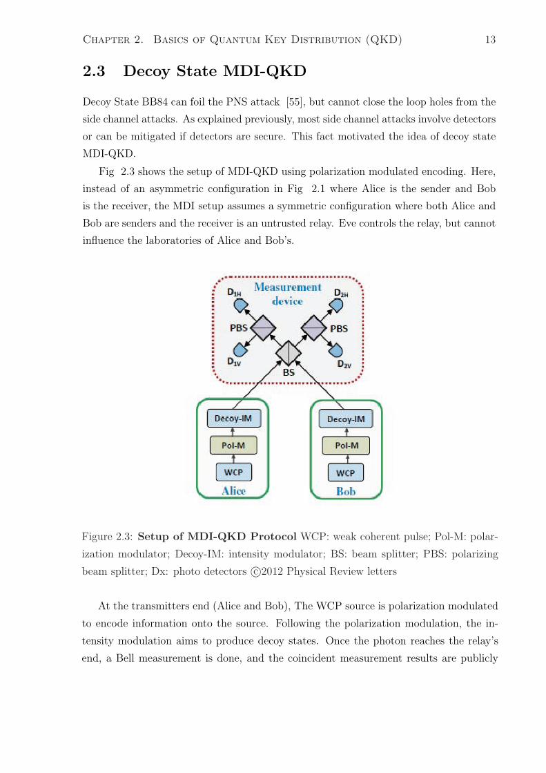
2.3 Decoy State MDI-QKD
Decoy State BB84 can foil the PNS attack [55], but cannot close the loop holes from the
side channel attacks. As explained previously, most side channel attacks involve detectors
or can be mitigated if detectors are secure. This fact motivated the idea of decoy state
MDI-QKD.
Fig 2.3 shows the setup of MDI-QKD using polarization modulated encoding. Here,
instead of an asymmetric configuration in Fig 2.1 where Alice is the sender and Bob
is the receiver, the MDI setup assumes a symmetric configuration where both Alice and
Bob are senders and the receiver is an untrusted relay. Eve controls the relay, but cannot
influence the laboratories of Alice and Bob’s.
Figure 2.3: Setup of MDI-QKD Protocol WCP: weak coherent pulse; Pol-M: polar-
ization modulator; Decoy-IM: intensity modulator; BS: beam splitter; PBS: polarizing
beam splitter; Dx: photo detectors c©2012 Physical Review letters
At the transmitters end (Alice and Bob), The WCP source is polarization modulated
to encode information onto the source. Following the polarization modulation, the in-
tensity modulation aims to produce decoy states. Once the photon reaches the relay’s
end, a Bell measurement is done, and the coincident measurement results are publicly
Chapter 2. Basics of Quantum Key Distribution (QKD) 14
announced to Alice and Bob.
The astute readers will notice that MDI foils the detector side channels. To see why,
we recognized that Bell measurements only result in the correlation of the bit streams,
but Eve cannot gain information because the message of logic bit 1 and logic bit 1
respectively from Alice and Bob respectively is as correlated as the message of logic bit
0 and logic bit 0 respectively from Alice and Bob respectively.
The secure key rate of MDI-QKD in the asymptotic case is given by [37]:
R ≥ PZ11Y
z11[1−H2(e
X11)]−QZ
µµfe(EZµµ)H2(E
Zµµ) (2.6)
Here the superscript Z or X indicates rectilinear basis or diagonal basis. PZ11 is the
probability of single photon states in Z basis. H2(x) = −xlog2(x)− (1− x)log2(1− x) is
the binary entropy functions. QZµµ and EZ
µµ denote the gain and QBER in the Z basis.
fe ≥ 1 is the error correction inefficiency function. µ is the optimal intensity of the signal
state in the asymptotic case.
Notice that compared to BB84, in MDI-QKD, the gain is not a detection probability,
but rather it is a co-incident registration probability. Also, Z basis is used for key
generation [56], whereas X is for testing purpose only [2, 46, 9, 3, 45].
As a summary, in MDI-QKD, the decoy state equations become [40, 37]:
Qλqa,qb
=∑
n,m=0
e−(qa+qb)qna
n!
qmb
m!Y λ
nm,
Qλqa,qb
Eλqa,qb
=∑
n,m=0
e−(qa+qb)qna
n!
qmb
m!Y λ
nmeλnm
(2.7)
where λ ∈ X,Z denotes the basis choice, qa(qb) denotes Alice’s (Bob’s) intensity set-
ting, Qλqa,qb
(Eλqa,qb
) denotes the gain (QBER) and Y λnm(eλ
nm denotes the yield (conditional
probability) (error rate) given Alice Bob send n-photon and m-photon respectively.
The tasks of decoy state MDI-QKD are to estimate a lower bound for Y Z11 and an
upper bound for eX11 using these linear equations. the optimal bound results are denoted
Y Z,L11 and eX,U
11 .
The goal of my M.A.Sc work is to improve the key rate of MDI-QKD protocols,
and this can be done in two ways. First, given the technological constraints, we want
to extract the most performance out of the current generation of the technology. My
first project on parameter optimization of the protocol focused on improving key rate
without modifying technology. Secondly, we can achieve higher key rate by using a better
technology. My second project on device characterization focused on purposing a better
Chapter 2. Basics of Quantum Key Distribution (QKD) 15
technology without the specification of how the technology is used. Together, the two
combined methodology will allow the achievement of highest key rate by exploiting the
best performance out of the most advanced technology.
2.4 Convex Optimization
All communication protocols involve some parameters. In the famous Internet Protocols
(IP) suite, the important parameters are packet size, number of hop, fragment offset and
etc. QKD as a physical layer protocol requires parameter optimization. In particular, a
decoy state MDI-QKD protocol is parameterized by:
• µ, the signal intensity
• ν, ω, ..., decoy states intensity
• Pµ,the probability of signal state
• Pν , Pω, ..., probability of decoy states
• PZ|µ, PX|µ, probability of basis in signal states
• PZ|ν , PX|ν , PZ|ω, PX|ω, ..., probability of basis in decoy states
• N , the total number of signal sent by both Alice and Bob; this parameter affect
the statistical fluctuation in experiment.
• d, the length of the fiber from Alice or Bob to the relay; this parameter in turn
determines the number of loss photon
with constraints:
• P ′s ≥ 0, P ′s ≤ 1
• Pµ + Pν + Pω = 1,
• PZ|µ + PX|µ = 1,
• PZ|ν + PX|ν = 1,
• PZ|ω + PX|ω = 1,
Chapter 2. Basics of Quantum Key Distribution (QKD) 16
The optimization procedure is effectively a search over these parameters.Depending
on how the optimization is done, the key rate as objective and/or the computation
resource requirements can be very different.The goal is to come close to the optimal
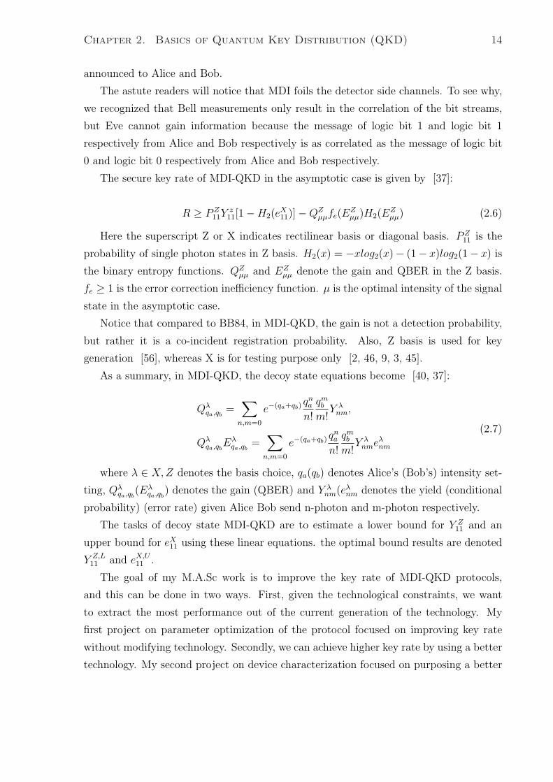
objective point, and the equal error contour (fig 2.4) is an effective way of visualizing
the progress we made as searching. The points on the same elliptical contour represent
the set of points with the same achieved objective value of Eqn 2.7. The contour is
usually elliptical is due to the use of Euclidean Norm.
Figure 2.4: Error Contour e1,e2: one of the dimensions of the optimization. All points
on the same ellipse have the same error, where the error of a point is quantified by how
far (in euclidian distance) the point is from the theoretical optimal point. The larger the
radius of the ellipse, the larger the error, (again) quantified by the euclidean distance
away from the optimality, the dot represent 0 error or optimality.
There are two well established methods in searching: exhaustive search and local
search [57].
2.4.1 Exhaustive Search
The exhaustive search is the most primitive methodology to search the entire search
space point-by-point. fig 2.5 shows that an exhaustive search is equivalent to laying out
a multi-dimensional grid and evaluating the objective at each point.
Prior to our publication in [45], all other optimizations [3, 46, 2] are done using
exhaustive search, and there are two salient drawbacks of this approach: On one hand, if
the search is too coarse, we may miss out the details completely and get a low key rate.
On the other hand, if the search is too fine, the search may take too long and become
Chapter 2. Basics of Quantum Key Distribution (QKD) 17
Figure 2.5: Exhaustive Search e1,e2: one of the dimensions of the optimization. A two
dimensional grid as illustration, this algorithm evaluate objective on all of the interior
points of the search space
infeasible in practical.
The problems to exhaustive search is that: there is no way to optimally lay out a
grid a priori without knowing the scaling features of the underlying topology. The niche
to be filled is a systematic and methodical procedure to traverse the search space and
automatically adopt to the scale of underlying topology.
2.4.2 Local Search
Local search is a suite of algorithms that aim to expedite the speed of the search by only
traversing the search that are “ relevant”. This suite includes the well-known steepest de-
scent (SD) algorithm and others such as conjugate descent algorithms. Here, I proposed
to use a non-derivative approximation to SD, the Coordinate Descent (CD) algorithm.
The non-derivative nature of the CD comes with many advantages in protocol optimiza-
tion. Firstly, protocol optimization involves simulations of the experiment. Hence, the
key rate as an objective is often an implicit function of the parameters and the actual
finding of the Gradients and Hessians of SD cannot be done easily. CD converges to the
same optimal point as SD, but may involve more iterations than SD.
To reduce both computational time and storage space requirements, I proposed to
use a combination of Coordinate Descent (CD) with Backtrack Search (BS) algorithm
[57]. The search trajectory of this particular local search algorithm is shown in Fig 2.6.
The following exposition of local search is largely based on [58]: The idea of CD is to
minimize the multivariate function objective (key rate R) by minimizing it along one
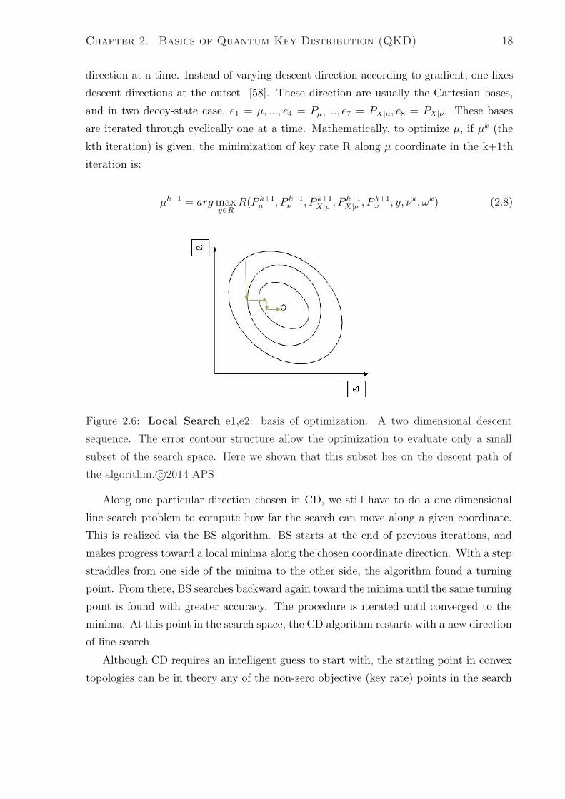
Chapter 2. Basics of Quantum Key Distribution (QKD) 18
direction at a time. Instead of varying descent direction according to gradient, one fixes
descent directions at the outset [58]. These direction are usually the Cartesian bases,
and in two decoy-state case, e1 = µ, ..., e4 = Pµ, ..., e7 = PX|µ, e8 = PX|ν . These bases
are iterated through cyclically one at a time. Mathematically, to optimize µ, if µk (the
kth iteration) is given, the minimization of key rate R along µ coordinate in the k+1th
iteration is:
µk+1 = arg maxy∈R
R(P k+1µ , P k+1
ν , P k+1X|µ , P k+1
X|ν , P k+1ω , y, νk, ωk) (2.8)
Figure 2.6: Local Search e1,e2: basis of optimization. A two dimensional descent
sequence. The error contour structure allow the optimization to evaluate only a small
subset of the search space. Here we shown that this subset lies on the descent path of
the algorithm. c©2014 APS
Along one particular direction chosen in CD, we still have to do a one-dimensional
line search problem to compute how far the search can move along a given coordinate.
This is realized via the BS algorithm. BS starts at the end of previous iterations, and
makes progress toward a local minima along the chosen coordinate direction. With a step
straddles from one side of the minima to the other side, the algorithm found a turning
point. From there, BS searches backward again toward the minima until the same turning
point is found with greater accuracy. The procedure is iterated until converged to the
minima. At this point in the search space, the CD algorithm restarts with a new direction
of line-search.
Although CD requires an intelligent guess to start with, the starting point in convex
topologies can be in theory any of the non-zero objective (key rate) points in the search
Chapter 2. Basics of Quantum Key Distribution (QKD) 19
space. In practice, prior research can shed light on the choices of initial parameters, and
these parameters often are good candidates for the starting guess.
2.5 Superconducting Nanowire Single Photon De-
tector
Making a detector sensitive to a quantum of light is by no mean an easy task, and to
characterize the sensitivity of a detector is also a challenging task. This section highlights
the most important parameters of a single photon detector (SPD).
Before tackling the exposition of different parameters, it is imperative to understand
what constitutes an ideal detector. A perfect detector is one that: 1) captures every
incoming photon 2) with perfect timing information, 3) no spontaneous or spurious reg-
istration (no dark count), 4) recovers (or quenching) from a detection instantaneous 5)
with no memory effect (afterpulsing), and last but not least, 6) the detector should be
able to tell the difference of n VS n+1 photons, as opposed to only make distinction of
0 and n¿0 photons.
I stress the fact that such an ideal detector does not exist, and the imperfections
of detector influence the performance of QKD protocols. It is the work of protocol
designers to factor these imperfections into the protocols and make an effort to minimize
these imperfections. The following introduction to these imperfection are summarized
from reference [51].
2.5.1 Detection Efficiency
In the probabilistic realm of Quantum Mechanics, not every photon is detected. The
detection efficiency of the detector captures the likelihood of a detector to register a pho-
ton. Detection efficiency varies with technology and with the wavelength of the photon,
and typical values of detection efficiency range from 0.15 for commonplace detector to
0.55 for superior devices [59]. For telecom fiber application, the detection efficiency at
1550nm is the lowest. High detection efficiency is a bonus but is not a requirement.
2.5.2 Dark Count Rate
Detection efficiency captures the probability of miss a photon (false negative), and its dual
concept of Dark Count Rate (DCR) captures the probability of registration of photon in
Chapter 2. Basics of Quantum Key Distribution (QKD) 20
the absence of any photons (false positive). Typical values of DCR may range from 1e-5
to 5e-5 [59], and too low a DCR could potentially enhance the performance of a QKD
system.
2.5.3 Dead Time
Realistic detector cannot register two consecutive photons with arbitrary time resolution.
The dead time of the detector is the required time for the detector to recover to original
state after detection. Typical values for dead time is 10ns to 20ns [59], and the minimal
dead time dictates the maximal repetition rate of the QKD system.
2.5.4 Timing Jitter
Figure 2.7: Effect of Timing Jitter The uncertainty of edge transition take away a
portion of the period. The actual (useful) period is smaller than the nominal (ideal)
period.
Timing jitter captures the time delay from the absorption of the photon optically to
the registration of detection electronically. Technically as in Fig 2.7, this jitter consume a
portion of the clock periods and reduces the maximum clock rate of the QKD experiment.
2.5.5 Afterpulsing
All of the previous imperfections affect the detector within one period of the repetition
rate. The relatively new concept of afterpulsing is a memory effect that spans multiple
periods. Afterpulsing refers to the increased probability of dark count rate at a prescribed
Chapter 2. Basics of Quantum Key Distribution (QKD) 21
time after the registration of a photon. It is desirable to eliminate afterpulse to increase
the repetition rate of the QKD system.
2.5.6 Number Resolving Detector VS. Threshold Detector
Number resolving detector is able to report the quantity of a photon stream, but threshold
detector can only report the presence of a photon stream. Threshold detectors are inferior
to number resolving detectors, but are the norm rather than the exception in today’s
technology.
Chapter 3
Protocol Parameter Optimization
This chapter is largely based on the article titled “ Protocol choice and parameter opti-
mization in decoy-state measurement-device-independent quantum key distribution” by
Feihu Xu, He Xu and Hoi-Kwong Lo, published in the Journal of Physical Review A.
The Journal of Physical Review A is published by the institute American Institute of
Physics. As such, copyright of this work belongs to the American Institute of Physics.
In this chapter, I will discuss the methodology and results of parameter optimization.
The aim is allow reader to understand the improvements in both the key rate and the
computational resources saving owing to the benefit of optimization.
The results presented here allow other researchers to make methodical judgements on
how to choose the number of decoy states, and given the number of decoy states how to
choose the parameter sets (intensities and probabilities) to optimize key rate.
The following physical constants and hardware parameters are used throughout this
chapter:
ηd ed Y0 fe ε N
14.5 % 1.5 % 6.02× 10⁻⁶ 1.16 10−7 1012
Table 3.1: Parameters and Constants, ηd: detection efficiency; ed: misalignment
error;Y0: background rate; fe: efficiency of error correction; ε: security parameter; N:
number of signal; Parameters are from QKD experiment [1]. In the experiment, two
SPDs are used. We assume four SPDs in MDI-QKD have identical ηd and Y0.
22
Chapter 3. Protocol Parameter Optimization 23
3.1 Convex Topology
Prior to the use of local search as a parameter optimization procedure, one must make
sure that the search space is continuous and convex. Continuity of search space is usually
implied by physics, as physical processes (except for black holes) usually vary smoothly
and rarely exhibit singular behavior. In contrast, convexity is usually an exception rather
than a norm.
The CD plus BS algorithm works in any general topology of the search space, but the
saving in efficiency comes only when the underlying topology, a.k.a. search domain, is a
convex optimization problem [57]. It is our goal here to demonstrate the convexity of the
key rate as a function of the parameters. The setting we adopt is a 2 decoy states protocol
for N=1012. Fig 3.1 demonstrates the convexity by noting that as the parameters µ and
ν are swept while other parameters are optimized over, the shape of the objective key
rate R is smooth and single-mounted.
Figure 3.1: Convexity of key rate function, topology is mapped by sweeping µ and
ν, and optimizing other parameters c©2014 APS
Even though this 2-D sweep cannot guarantee the convexity of the entire 13 dimen-
sion, I remark here that the non-convexity of the overall topology only brings down the
efficiency of the search. The CD plus BS algorithm will still work in a non-convex domain,
and the subsequent improved results shed lights on the convexity of the domain.
3.2 Computational Resource
Optimization of parameters is a routine for almost all of the proposed protocols. However
the sheer size of the search space bring a “ curse of dimension” nightmare. In higher
Chapter 3. Protocol Parameter Optimization 24
dimensions, especially with computational resource (time and space) constraints, it is
only possible to explore a (intelligent) subspace of the search space. This limitation
will in turn induces one form of sub-optimality or another. Hence there is a stringent
demand for a computationally light-weight yet accurate enough algorithm to probe the
entire search space. The availability of such procedure will not only improve numerical
recipe in term of programming, but will also shed light on how the protocols behave
under proper changes of parameters.
Since I have proposed to use CD plus BS for searching, it is imperative to compare the
speed and accuracy of local search (LS) to exhaustive search (ES) algorithm. I remark
here that the claimed large improvement in speed does come with a complexity cost.
Any LS will have the need to maintain complex neighborhood relational logic compared
to primitive nested loop structure of the EA. Hence, without significant advantages, the
complexity of LS will not be justified.
The comparison of results in table 3.2 clearly indicate that LS shows 4 order of
magnitude improvement over ES while maintaining the same degree of accuracy.
Method Iterations Time Key rate
Exhaustive search 107 550 hours 6.84× 10⁻⁵
Local search 33 1 min 6.83× 10⁻⁵
Table 3.2: Speed and Accuracy Comparison, Simulation is on MDI-QKD with two
decoy-state numerical approach on a standard desktop computer. A full optimization on
eight dimension (intensity and probability) is performed. ω is fixed at a near optimal
ω=0.0005. The grid for exhaustive search is 10 points per dimension for a total of 107
iteration. c©2014 APS
3.3 Key Rate Comparison between Optimization
and Non-optimization
As mentioned that, to date, there is no unified framework to choose parameters, most
of the previous work either empirically choose some typical parameters as in [27,29] or
only perform a partial optimization on a subset of parameters (i.e. only intensity) or
only on a restricted sub-domain of the search space. All these approximations to a full
Chapter 3. Protocol Parameter Optimization 25
optimization is directly or indirectly owing to the complexity in searching in a large (as
many as 8-15) dimensional space.
Now, our proposed local search algorithm solves the complexity problem, and it is
our purpose to illustrate the difference between a full optimized key rate and a partially
optimized key rate.
Fig 3.2 compare our optimization to those using the parameters and methods pre-
sented in Refs [27,29,30] in asymptotical case. From this figure, we make a few observa-
tions (and conclusion):
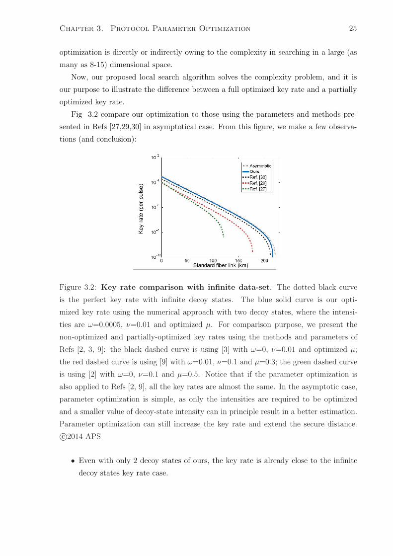
Figure 3.2: Key rate comparison with infinite data-set. The dotted black curve
is the perfect key rate with infinite decoy states. The blue solid curve is our opti-
mized key rate using the numerical approach with two decoy states, where the intensi-
ties are ω=0.0005, ν=0.01 and optimized µ. For comparison purpose, we present the
non-optimized and partially-optimized key rates using the methods and parameters of
Refs [2, 3, 9]: the black dashed curve is using [3] with ω=0, ν=0.01 and optimized µ;
the red dashed curve is using [9] with ω=0.01, ν=0.1 and µ=0.3; the green dashed curve
is using [2] with ω=0, ν=0.1 and µ=0.5. Notice that if the parameter optimization is
also applied to Refs [2, 9], all the key rates are almost the same. In the asymptotic case,
parameter optimization is simple, as only the intensities are required to be optimized
and a smaller value of decoy-state intensity can in principle result in a better estimation.
Parameter optimization can still increase the key rate and extend the secure distance.
c©2014 APS
• Even with only 2 decoy states of ours, the key rate is already close to the infinite
decoy states key rate case.
Chapter 3. Protocol Parameter Optimization 26
• key rates without parameter optimization in Refs [27.29] are an order of magnitude
lower than ours and than in [30] with optimization.
• there is still a 50 % gap in key rate between partially optimized key rate in [30]
and a fully optimized key rate in ours.
• the increased key rate is also accompanied by a extension of secure distance
There are relatively fewer parameters (only intensity) in asymptotical cases, but in
finite key cases, it is to be expected that greater number of parameter can make the
improvements (compared to partially optimized) in optimized key rate much higher
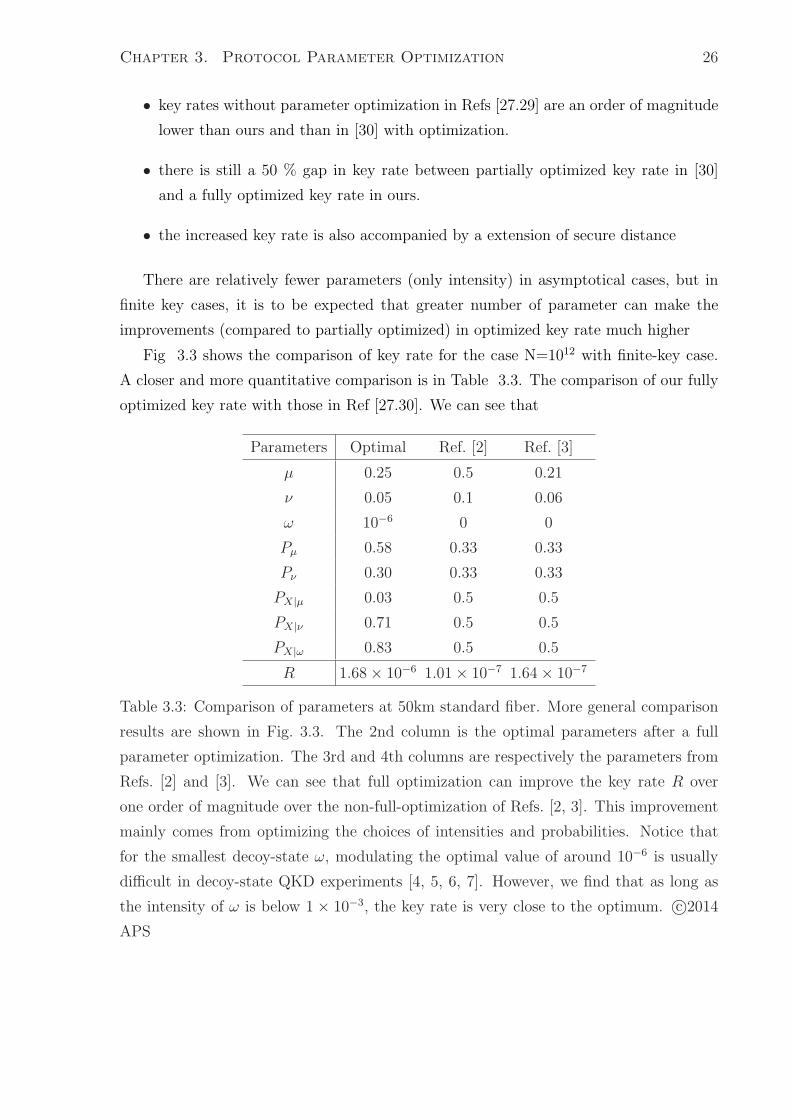
Fig 3.3 shows the comparison of key rate for the case N=1012 with finite-key case.
A closer and more quantitative comparison is in Table 3.3. The comparison of our fully
optimized key rate with those in Ref [27.30]. We can see that
Parameters Optimal Ref. [2] Ref. [3]
µ 0.25 0.5 0.21
ν 0.05 0.1 0.06
ω 10−6 0 0
Pµ 0.58 0.33 0.33
Pν 0.30 0.33 0.33
PX|µ 0.03 0.5 0.5
PX|ν 0.71 0.5 0.5
PX|ω 0.83 0.5 0.5
R 1.68× 10⁻⁶ 1.01× 10⁻⁷ 1.64× 10⁻⁷
Table 3.3: Comparison of parameters at 50km standard fiber. More general comparison
results are shown in Fig. 3.3. The 2nd column is the optimal parameters after a full
parameter optimization. The 3rd and 4th columns are respectively the parameters from
Refs. [2] and [3]. We can see that full optimization can improve the key rate R over
one order of magnitude over the non-full-optimization of Refs. [2, 3]. This improvement
mainly comes from optimizing the choices of intensities and probabilities. Notice that
for the smallest decoy-state ω, modulating the optimal value of around 10−6 is usually
difficult in decoy-state QKD experiments [4, 5, 6, 7]. However, we find that as long as
the intensity of ω is below 1 × 10⁻³, the key rate is very close to the optimum. c©2014
APS
Chapter 3. Protocol Parameter Optimization 27
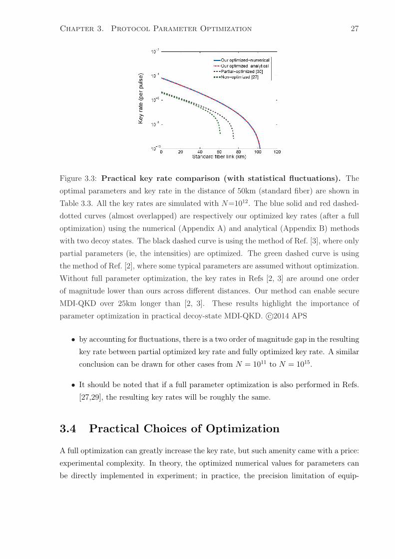
Figure 3.3: Practical key rate comparison (with statistical fluctuations). The
optimal parameters and key rate in the distance of 50km (standard fiber) are shown in
Table 3.3. All the key rates are simulated with N=1012. The blue solid and red dashed-
dotted curves (almost overlapped) are respectively our optimized key rates (after a full
optimization) using the numerical (Appendix A) and analytical (Appendix B) methods
with two decoy states. The black dashed curve is using the method of Ref. [3], where only
partial parameters (ie, the intensities) are optimized. The green dashed curve is using
the method of Ref. [2], where some typical parameters are assumed without optimization.
Without full parameter optimization, the key rates in Refs [2, 3] are around one order
of magnitude lower than ours across different distances. Our method can enable secure
MDI-QKD over 25km longer than [2, 3]. These results highlight the importance of
parameter optimization in practical decoy-state MDI-QKD. c©2014 APS
• by accounting for fluctuations, there is a two order of magnitude gap in the resulting
key rate between partial optimized key rate and fully optimized key rate. A similar
conclusion can be drawn for other cases from N = 1011 to N = 1015.
• It should be noted that if a full parameter optimization is also performed in Refs.
[27,29], the resulting key rates will be roughly the same.
3.4 Practical Choices of Optimization
A full optimization can greatly increase the key rate, but such amenity came with a price:
experimental complexity. In theory, the optimized numerical values for parameters can
be directly implemented in experiment; in practice, the precision limitation of equip-
Chapter 3. Protocol Parameter Optimization 28
ments (modulator, RNG’s) precludes the use of optimal parameters set. Furthermore,
the implementation of fully optimized parameters requires several replicas of the same
equipment; for example, 4 RNG’s are needed to implement the selection of signal/decoy
and the selection of basis for each signal and decoy state.
To query the extend of this limitation, we investigate three options in optimization:
1. unbiased basis choice, 2. simplified basis choice and 3. optimal basis choice. The most
basic unbiased basis choice is exactly the one adopted by standard protocol prior to our
publication. Here the basis for X and Z are all equal. this is the cheapest to implement
as there is no need for RNG’s. Next to unbiased comes the simplified basis choice, in
which the basis choice are independent of intensity. Hence only one RNG is needed to
control basis choice for both signal and decoys. Last but not least, optimal basis choice
make decisions on basis depending on intensity (signal VS decoys) of the choice. Here
for 2 decoy states, 3 RNG’s are needed to fully control the basis. In addition, the extra
RNG used to do state selection must be synchronized with the 3 basis choice RNG as
the selection is intensity dependent.
Mathematically, these kinds of hardware limitations are translated as optimization
constraints summarized here:
• unbiased choice: PX|µ = PX|ν = PX|ω = 12
= PZ|µ = PZ|ν = PZ|ω
• simplified choice: PX|µ = PX|ν = PX|ω and, PZ|µ = PZ|ν = PZ|ω
• optimized choice: no constraint
Table 3.4 shows the comparison results for different choices of bases. The result is
obtained using numerical method. The conclusion to draw from these data are:
• The Optimal choice are 300% ish higher than unbiased choice
• The optimal choice are 200% ish higher than those of simplified choice
• The smaller the data size, the more prominent in key rate gain from a full opti-
mization
• The ease of implementation of unbiased choice is not justified with the dramatic
loss in key rate.
Chapter 3. Protocol Parameter Optimization 29
Distance 0km 0km 0km 50km 50km 50km
Data-size 1012 1014 1018 1012 1014 1018
Unbiased 1.50× 10⁻⁵ 3.98× 10⁻⁵ 6.37× 10⁻⁵ 3.21× 10⁻⁷ 2.39× 10⁻⁶ 5.71× 10⁻⁶
Simplified 2.05× 10⁻⁵ 6.27× 10⁻⁵ 2.03× 10⁻⁴ 3.36× 10⁻⁷ 3.97× 10⁻⁶ 1.66× 10⁻⁵
Optimal 6.83× 10⁻⁵ 1.72× 10⁻⁴ 2.72× 10⁻⁴ 1.68× 10⁻⁶ 1.05× 10⁻⁵ 2.24× 10⁻⁵
Distance 100km 100km 100km
Data-size 1012 1014 1018
Unbiased 0 9.88× 10⁻⁸ 4.72× 10⁻⁷
Simplified 0 1.28× 10⁻⁷ 1.21× 10⁻⁶
Optimal 6.05× 10⁻¹⁰ 4.61× 10⁻⁷ 1.78× 10⁻⁶
Table 3.4: Key rate values with different basis choices. The key rates are simulated with
two decoy states and numerical approach. Unbiased denotes the standard protocol with
equal basis choice; Simplified denotes the simplified choice with the (biased) basis choice
independent of intensity choice; Optimal denotes the optimal choice with the (biased)
basis choice depending on intensity choice. In a large data-set of 1018 (approaching
asymptotic case), the key rates with optimal choice are around 300% higher than those
of unbiased choice and close to those of simplified choice. In a reasonable data-set (1012 to
1014), the key rates with optimal choice are around 300% higher than those of unbiased
choice and around 200% higher than those of simplified choice. This shows that the
optimal choice can significantly increase the key rates in a practical setting with finite
data-set. c©2014 APS
3.5 Choosing the Number of Decoy
Having established the framework for parameter optimization, I now address the second
major question of MDI-QKD: how many decoy states should I use. Superficially, increas-
ing the number of decoy states always improves key rate; however, the minute increase
in key rate cannot justify the unduely growth of hardware complexity.
The results of numerical optimization for different numbers of decoy states are in Figs
3.4, 3.5 and 3.5. From these data, I make the following observations:
• after a full parameter optimization, two decoy states can give an almost optimal
key rate,
• using three decoy states cannot improve much but using one decoy state is severely
sub-optimal
Chapter 3. Protocol Parameter Optimization 30
Figure 3.4: (Color online) Asymptotic key rates with different number of decoy states.
The solid curve is the one with infinite decoy states. The dashed, dashed-dotted, dotted
curves are respectively the one, two, three decoy-state results using numerical methods
(see Appendix A). The signal state µ is optimized in all cases, while some reasonable
values of decoy states are adopted: for one decoy state, ν=0.0005; for two decoy states,
ν=0.01 and ω=0.0005; for three decoy states, ν1=0.1, ν2=0.01 and ω=0.0005. We em-
phasize that the key rates with analytical methods of Appendix B are almost overlapped
with the ones presented in this figure, which shows that the analytical approaches pro-
vide a highly good estimation. The estimation using two decoy states gives a nearly
similar key rate to the one with three decoy states and is higher than one decoy-state
case. Therefore, two decoy states can already result in a near optimal estimation and
more decoy states cannot improve the key rate. c©2014 APS
• After a full optimization, the numerical and analytical methods are without large
gap. Hence, analytical method gives good state estimation and the improvement
of numerical over analytical estimation reported in [27,29,30] disappeared in a fully
optimized parameters set.
3.6 Effect of the smallest decoy state ω
While a full optimization gives distinct values for parameter as N and d are changed, but
in practice the finite extinction ratio below 30dB cannot be generated with an intensity

Chapter 3. Protocol Parameter Optimization 31
Figure 3.5: (Color online) Secret key rate in logarithmic scale as a function of the distance
under different numbe of decoy states. The main figure is for data-set N=1012 and the
inserted figure is for N=1014. The key rates are obtained using numerical methods with
one (dashed curve), two (solid curve), three (dashed-dotted curve) decoy states. The key
rates with two and three decoy states are almost overlapped. In simulation, we perform
a full parameter optimization for all cases. Our results show that after a full parameter
optimization, the two decoy-state method can give an almost optimal key rate, which is
higher than the one with one decoy state. Three decoy states cannot help to increase the
key rate. c©2014 APS
modulator [5, 6]. As shown in Ref [2], there is a benefit to include a “ vacuum” decoy,
and it is highly desirable to not modulate the smallest “ vacuum” decoy’s intensity, but
fixed it at the lowest extinction ratio can be achieved with today’s technology.
Fig 3.6 presents the investigation of the effect of the smallest vacuum state. The
simulation is performed by sweeping the smallest intensity ω while optimize the other
parameters.
The figure indicates the optimal value of ω is always in the vicinity of 5× 10⁻⁶. The
conclusion is: as long as the intensity of ω is below 1 × 10⁻³, the key rate is very close
to the optimum, and a perfect vacuum (ω = 0) is not required in a practical decoy state
QKD experiment.

Chapter 3. Protocol Parameter Optimization 32
Distance 0km 0km 0km 50km 50km 50km
Data-size 1012 1014 ∞ 1012 1014 ∞1decoy-Num 8.10× 10⁻⁶ 1.41× 10⁻⁵ 3.59× 10⁻⁵ 2.56× 10⁻⁷ 9.34× 10⁻⁷ 3.03× 10⁻⁶
2decoy-Num 6.83× 10⁻⁵ 1.72× 10⁻⁴ 3.25× 10⁻⁴ 1.68× 10⁻⁶ 1.05× 10⁻⁵ 2.95× 10⁻⁵
2decoy-Ana 6.65× 10⁻⁵ 1.67× 10⁻⁴ 3.25× 10⁻⁴ 1.67× 10⁻⁶ 1.01× 10⁻⁵ 2.95× 10⁻⁵
3decoy-Num 6.76× 10⁻⁵ 1.71× 10⁻⁴ 3.03× 10⁻⁴ 1.66× 10⁻⁶ 1.04× 10⁻⁵ 2.92× 10⁻⁵
Distance 100km 100km 100km
Data-size 1012 1014 ∞1decoy-Num 0 4.64× 10⁻⁸ 2.41× 10⁻⁷
2decoy-Num 6.05× 10⁻¹⁰ 4.61× 10⁻⁷ 2.98× 10⁻⁶
2decoy-Ana 5.97× 10⁻¹⁰ 4.48× 10⁻⁷ 2.77× 10⁻⁶
3decoy-Num 6.02× 10⁻¹⁰ 4.55× 10⁻⁷ 2.70× 10⁻⁶
Table 3.5: Optimal key values under different number of decoy states. With finite data-
set, the key rates with two decoy states are around one order of magnitude higher than
the ones with one decoy state. Three decoy states cannot help to improve the key
rates. Hence, two decoy states can achieve a near optimal key rate. In the case of two
decoy states, the numerical method (Num) can only improve the key around 2% over the
ones using our analytical method (Ana). This shows that the two decoy-state analytical
method presented in Appendix B can also result in a near optimal estimation. c©2014
APS
3.7 Asymmetric MDI-QKD
MDI-QKD can be analyzed in a symmetric setting, where the transmission distances
from Alice’s or Bob’s laboratory to the measurement device blackbox are equal, but a
more practical scenario would correspond to asymmetry settings, where the transmission
distances are not equal. As it is not obvious how to choose the experimental parameters
in this case, I have conducted study on 3 methodologies using 2 decoy states at N = 1012:
1.simplified choice of parameter, which is totally different than the simplified basis choice
explained in Section 3.4 for symmetric setting, 2. symmetric choice of parameters, and
3 fully optimized choice of parameters.
In simplified choice of parameter, we assume the symmetric case’s result simply carry
over to asymmetric case. However, this simplification result in identically 0 key rate.
Hence, this brute force extension to asymmetric case proved to be wrong.
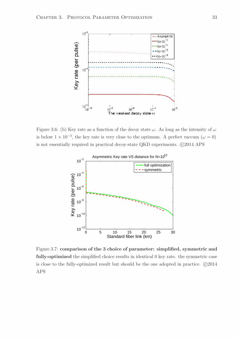
Chapter 3. Protocol Parameter Optimization 33
Figure 3.6: (b) Key rate as a function of the decoy state ω. As long as the intensity of ω
is below 1× 10⁻³, the key rate is very close to the optimum. A perfect vaccum (ω = 0)
is not essentially required in practical decoy-state QKD experiments. c©2014 APS
0 5 10 15 20 25 3010
−12
10−10
10−8
10−6
10−4
10−2
Standard fiber link (km)
Key
rat
e (p
er p
ulse
)
Asymmetric Key rate VS distance for N=1012
full optimizationsymmetric
Figure 3.7: comparison of the 3 choice of parameter: simplified, symmetric and
fully-optimized the simplified choice results in identical 0 key rate. the symmetric case
is close to the fully-optimized result but should be the one adopted in practice. c©2014
APS
Chapter 3. Protocol Parameter Optimization 34
In symmetric choice, the state probabilities and basis probabilities are chosen inde-
pendently for Alice and Bob, but to account for the asymmetric distance and loss, we
will scale both Bob’s signal and decoy intensity by tatb
in hope of this scaling will work
better. The result on key rate shows that this is indeed a good choice, but there is still a
gap away from the optimized choice of parameters. Mathematically, the constraints for
symmetric choice are:
• PAliceµ = PBob
µ , PAliceν = PBob
ν , PAliceω = PBob
ω
• PAliceX|µ = PBob
X|µ , PAliceX|ν = PBob
X|ν , PAliceX|ω = PBob
X|ω
Finally, the full optimized choice does a thorough optimization on both Alice’s pa-
rameters and Bob’s parameter independently. This requires twice as many parameters
as in the symmetric MDI-QKD case. The final result in 3.7 shows that the final key
rate is superior to the symmetric choice of parameters. Although superior, the improve-
ment of 30 percent of key rate does not justify the use of fully optimized result in actual
experiment. Moreover, the improvement of tolerant distance from 26km to 30km also
cannot dispense us from a quantum repeaters. Hence, for all purposes, symmetric choice
of parameter is a good compromise between experimental complexity and performance.
Our analysis on the improvement of key rate and tolerant distance shows the root
cause of the improvement is the better estimation of e11, and this is accomplished by
the lowering of signal state probability Pµ in exchange for the decoy state probability Pν
and Pω
3.8 Summary
This section summarize the results on optimization by a series of Questions & Answers
Q1: How do I know my optimization is convex?
A1: If the optimization is done on physical parameters, the smoothness is guaran-
teed by physics, and non-convexity will bring down the efficiency of the algorithm, but
nonetheless produce reasonable key rate as objective.
Q2: Should I use Exhaustive Search (ES) or Local Search (LS)?
A2: Use a coarse grid ES to provide a sensible initial guess, and then run LS for
optimization to get huge saving on time.
Q3: Should I do partial optimization or a full optimization?
Chapter 3. Protocol Parameter Optimization 35
A3: With LS, a full optimization is hardly any more effort, hence always do full
optimization.
Q4: If I do have hardware limitation, what approximation scheme should I use?
A4: If aiming for a long fiber distance, use optimized basis choice for non-zero key
rate, but use simplified basis choice in case of severe hardware limitation.
Q5: How many decoy states should I use?
A5: The best number is 2 decoy states, as already shown that it is very much the
same key rate compared to the case of infinite decoy states
Q6: should I go to the trouble of modulating the smallest “ vacuum”?
A6: No, for all practical purposes, fix it at ω = 5× 10⁻⁶
Q7: If I just migrated from symmetric MDI-QKD to an asymmetric ones, what
additional effort should I do?
A7: use symmetric basis choice to both save computation parameters and additional
hardware.
3.9 Conclusion
Our work on the parameter optimization provided a local search recipe to explore the
entire domain of the search while maintaining a non-exponentially growing space and time
complexity. Also, our work resolved previous three un-answered questions in the QKD
community: First, we illustrated to other researchers that their optimization is only
partially done, and such in-complete optimizations will result in sub-optimal key rate
objectives. Second, our algorithm also presented the answer to what happen if hardware
limitation can allow only searching a sub-domain, e.g. when the smallest ”vaccum” can
only be 5× 10⁻⁶. Finally, and most importantly, our work prescribed the use of 2 decoy
states to get a near-optimal key rate, and more than two decoy states will result in
diminishing return. With these contributions, I believe our work has impacted the QKD
academia on the improvement of MDI-QKD protocols.
Chapter 4
Characterization of Single Photon
Superconducting Detector
This chapter is largely based on the article titled “ Investigations of Afterpulsing and
Detection Efficiency Recovery in SNSPDs” by Viacheslav Burenkov, He Xu, Bing Qi,
Robert H. Hadfield and Hoi-Kwong Lo, published in Journal of Applied Physics [51].
The Journal of Applied Physics is published by the American Institute of Physics. As
such, copyright of this work belongs to the American Institute of Physics.
This chapter is logically divided into two parts: the first part is done before my joining
of the project, and the second part of the project has my contribution. The experiment
in section 4.4 and 4.5 is done entirely by Viacheslav Burenkov, and the experiments in
section 4.6 4.7 and 4.8 are jointly done by He Xu and Viacheslav Burenkov. Finally,
the Simulink models in Appendix C can be replicated by readers who want to delve
deeper in validation of our results.
4.1 Introduction
Superconducting Nanowire Single Photon Detectors (SNSPDs) are a relatively new tech-
nology for detecting single infrared photons [60, 61]. They can offer certain advantages
over other single photon detectors due to their potentially short dead time, small timing
jitter [62] and low dark count rate [63]. As such, they have been used in many areas of
research, including quantum key distribution (QKD) [64, 65, 66, 67, 68, 69], quantum
state tomography [70] and other quantum optic experiments. There has been growing
interest in completely characterizing these quantum detectors through a process called
36
Chapter 4. Characterization of Single Photon Superconducting Detector37
detector tomography [71, 72, 73]. Yet, such characterization is often based on the re-
sponse of a detector to a one-shot input, when the initial state of a detector is “active”.
In other words, it does not consider the possibility that a detector is already “dead” due
to an earlier detection event (a “click”) and the fact that the response of a detector to a
signal actually depends on its initial state and when the last detection event occurs.
In the context of QKD, we remark that the existing theoretical models for photon
detectors are often too simplistic and do not take into account various imperfections in
practical detectors. This is highly undesirable because, for one thing, those imperfections
may open up security loopholes which allow Eve to hack commercial QKD systems, as
demonstrated by the recent quantum hacking experiments against InGaAs APDs [74, 75]
and an SNSPD [76]. Therefore, it is important to re-examine existing models for detectors
and see if they describe practical detectors well.
Regarding SNSPDs, two assumptions are often made. First, it is commonly assumed
without proof that the dark counts (spurious clicks that occur with no light input) of
an SNSPD are uniform in time. Secondly, initial experimental studies [77] indicate that
detection efficiency recovers continuously, mirroring the recovery of the bias current in
the nanowire [78].
In this thesis, we find that, rather surprisingly, both assumptions are invalid for
a practical SNSPD. Our investigation consists of three parts. In the first part of our
investigation, with no laser input, we study the distribution of dark counts. We find
that, rather unexpectedly, dark counts are not uniform. In fact, dark counts show a
clustering effect, which we refer to as “afterpulsing”. This “afterpulsing” can be triggered
by photons, or can also be triggered by un-intentional blackbody radiation when laser is
off. More concretely, for our SNSPD, the total dark count probability could be separated
into a uniformly distributed “pure” dark count probability and a highly time-dependent
“extra” dark count probability, occurring on a time scale of around 180 ns after a previous
dark count.
We found that the probability of afterpulsing of dark counts increases exponentially
as the bias current is increased. At high bias currents, afterpulsing of dark counts can be
an important contribution to the overall dark count rate. Besides, at high bias currents,
more than one afterpulse can occur, with a time interval of about 180 ns between the
adjacent afterpulses. At very high bias current, a long train of afterpulses can occur. We
study the distribution of the number of pulses as a function of bias current. We discuss
the implications of our finding on the security and performance of QKD with SNSPDs.
Chapter 4. Characterization of Single Photon Superconducting Detector38
In the second part of our investigation, with a pulsed laser on with a repetition
rate of 2 MHz, we study the distribution of detection events. We observe that about
180 ns following a real detection event due to an input pulse, there is an enhanced
probability for our SNSPD to register a (spurious) detection event. Such a spurious
detection event is commonly called an afterpulse. We note that two papers related to
afterpulsing in SNSPDs (with laser on) have been published recently [79, 80]. In Ref.
[79], the afterpulsing effect of an SNSPD with a laser input has been studied on the
time scale of 100 ns. Here, we study the afterpulsing effect with a laser input at a much
larger time-scale (of 1000 ns) and, for the first time, report the secondary afterpulsing
effect (the afterpulse of an afterpulse). Indeed, we find that about 180 ns after the first
afterpulse, there is an enhanced probability of having a second afterpulse. This is similar
to our finding in the first part of our investigation (with no laser input).
In the third part of our investigation, we study the recovery curve of SNSPD after
a detection event. Here, we report an unexpected recovery of detection efficiency after
a detector click. Contrary to the widespread belief, the detection efficiency does not
monotonically rise to its nominal value but instead increases beyond it on the same time
scale as the afterpulsing, before dropping back to the nominal value.
The chapters are structured as follows. Sec. 4.2 introduces the physics of SNSPD and
defines the afterpulse phenomenon. Sec. 4.3 describes our experimental set-up in detail
and defines what exactly constitutes a detection event. Sec. 4.4 presents our results of
a non-uniform distribution of the dark count events in the SNSPD, and introduces the
aforementioned afterpulse effect. In Sec. 4.5, we characterize the afterpulsing effect and
explain it as a reflection in the readout circuit used, as previously proposed in Ref. [79].
Analysis of afterpulsing is then extended to experiments with incoming light in Sec. 4.6.
In Sec. 4.7 we present our results of detection efficiency recovery following a detection
event, showing an unexpected temporary rise in detection efficiency beyond the nominal
value. In Sec. 4.8 we demonstrate experimentally that afterpulsing can be eliminated by
using a different amplifier. Finally, we make a summary and concluding comments in
Sec. 4.9, including highlighting the significance of using an SNSPD with these properties
for QKD.
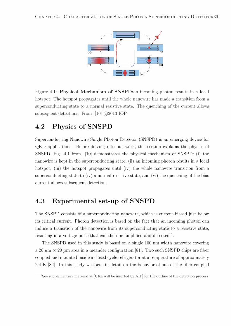
Chapter 4. Characterization of Single Photon Superconducting Detector39
Figure 4.1: Physical Mechanism of SNSPD:an incoming photon results in a local
hotspot. The hotspot propagates until the whole nanowire has made a transition from a
superconducting state to a normal resistive state. The quenching of the current allows
subsequent detections. From [10] c©2013 IOP
4.2 Physics of SNSPD
Superconducting Nanowire Single Photon Detector (SNSPD) is an emerging device for
QKD applications. Before delving into our work, this section explains the physics of
SNSPD. Fig 4.1 from [10] demonstrates the physical mechanism of SNSPD: (i) the
nanowire is kept in the superconducting state, (ii) an incoming photon results in a local
hotspot, (iii) the hotspot propagates until (iv) the whole nanowire transition from a
superconducting state to (iv) a normal resistive state, and (vi) the quenching of the bias
current allows subsequent detections.
4.3 Experimental set-up of SNSPD
The SNSPD consists of a superconducting nanowire, which is current-biased just below
its critical current. Photon detection is based on the fact that an incoming photon can
induce a transition of the nanowire from its superconducting state to a resistive state,
resulting in a voltage pulse that can then be amplified and detected 1.
The SNSPD used in this study is based on a single 100 nm width nanowire covering
a 20 µm × 20 µm area in a meander configuration [81]. Two such SNSPD chips are fiber
coupled and mounted inside a closed cycle refrigerator at a temperature of approximately
2.4 K [82]. In this study we focus in detail on the behavior of one of the fiber-coupled
1See supplementary material at [URL will be inserted by AIP] for the outline of the detection process.
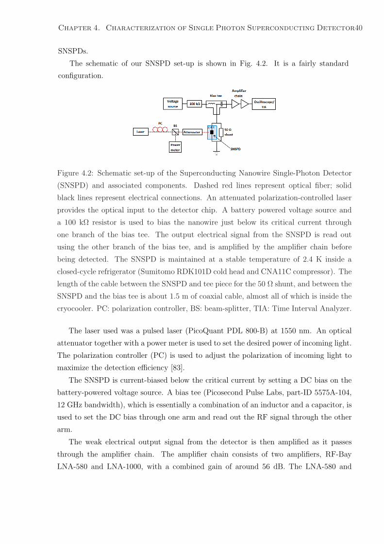
Chapter 4. Characterization of Single Photon Superconducting Detector40
SNSPDs.
The schematic of our SNSPD set-up is shown in Fig. 4.2. It is a fairly standard
configuration.
Figure 4.2: Schematic set-up of the Superconducting Nanowire Single-Photon Detector
(SNSPD) and associated components. Dashed red lines represent optical fiber; solid
black lines represent electrical connections. An attenuated polarization-controlled laser
provides the optical input to the detector chip. A battery powered voltage source and
a 100 kΩ resistor is used to bias the nanowire just below its critical current through
one branch of the bias tee. The output electrical signal from the SNSPD is read out
using the other branch of the bias tee, and is amplified by the amplifier chain before
being detected. The SNSPD is maintained at a stable temperature of 2.4 K inside a
closed-cycle refrigerator (Sumitomo RDK101D cold head and CNA11C compressor). The
length of the cable between the SNSPD and tee piece for the 50 Ω shunt, and between the
SNSPD and the bias tee is about 1.5 m of coaxial cable, almost all of which is inside the
cryocooler. PC: polarization controller, BS: beam-splitter, TIA: Time Interval Analyzer.
The laser used was a pulsed laser (PicoQuant PDL 800-B) at 1550 nm. An optical
attenuator together with a power meter is used to set the desired power of incoming light.
The polarization controller (PC) is used to adjust the polarization of incoming light to
maximize the detection efficiency [83].
The SNSPD is current-biased below the critical current by setting a DC bias on the
battery-powered voltage source. A bias tee (Picosecond Pulse Labs, part-ID 5575A-104,
12 GHz bandwidth), which is essentially a combination of an inductor and a capacitor, is
used to set the DC bias through one arm and read out the RF signal through the other
arm.
The weak electrical output signal from the detector is then amplified as it passes
through the amplifier chain. The amplifier chain consists of two amplifiers, RF-Bay
LNA-580 and LNA-1000, with a combined gain of around 56 dB. The LNA-580 and
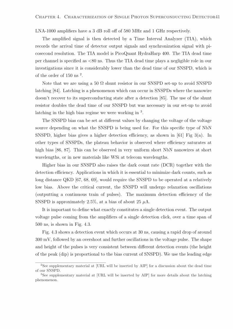
Chapter 4. Characterization of Single Photon Superconducting Detector41
LNA-1000 amplifiers have a 3 dB roll off of 580 MHz and 1 GHz respectively.
The amplified signal is then detected by a Time Interval Analyzer (TIA), which
records the arrival time of detector output signals and synchronization signal with pi-
cosecond resolution. The TIA model is PicoQuant HydraHarp 400. The TIA dead time
per channel is specified as <80 ns. Thus the TIA dead time plays a negligible role in our
investigations since it is considerably lower than the dead time of our SNSPD, which is
of the order of 150 ns 2.
Note that we are using a 50 Ω shunt resistor in our SNSPD set-up to avoid SNSPD
latching [84]. Latching is a phenomenon which can occur in SNSPDs where the nanowire
doesn’t recover to its superconducting state after a detection [85]. The use of the shunt
resistor doubles the dead time of our SNSPD but was necessary in our set-up to avoid
latching in the high bias regime we were working in 3.
The SNSPD bias can be set at different values by changing the voltage of the voltage
source depending on what the SNSPD is being used for. For this specific type of NbN
SNSPD, higher bias gives a higher detection efficiency, as shown in [61] Fig 3(a). In
other types of SNSPDs, the plateau behavior is observed where efficiency saturates at
high bias [86, 87]. This can be observed in very uniform short NbN nanowires at short
wavelengths, or in new materials like WSi at telecom wavelengths.
Higher bias in our SNSPD also raises the dark count rate (DCR) together with the
detection efficiency. Applications in which it is essential to minimize dark counts, such as
long distance QKD [67, 68, 69], would require the SNSPD to be operated at a relatively
low bias. Above the critical current, the SNSPD will undergo relaxation oscillations
(outputting a continuous train of pulses). The maximum detection efficiency of the
SNSPD is approximately 2.5%, at a bias of about 25 µA.
It is important to define what exactly constitutes a single detection event. The output
voltage pulse coming from the amplifiers of a single detection click, over a time span of
500 ns, is shown in Fig. 4.3.
Fig. 4.3 shows a detection event which occurs at 30 ns, causing a rapid drop of around
300 mV, followed by an overshoot and further oscillations in the voltage pulse. The shape
and height of the pulses is very consistent between different detection events (the height
of the peak (dip) is proportional to the bias current of SNSPD). We use the leading edge
2See supplementary material at [URL will be inserted by AIP] for a discussion about the dead timeof our SNSPD.
3See supplementary material at [URL will be inserted by AIP] for more details about the latchingphenomenon.
Chapter 4. Characterization of Single Photon Superconducting Detector42
0 100 200 300 400 500
−0.3
−0.25
−0.2
−0.15
−0.1
−0.05
0
0.05
0.1
0.15
Time (ns)
Out
put
(V)
experiment
detection threshold
Figure 4.3: Output pulse shape of a single detection click, starting at 30 ns, as observed
on an oscilloscope (rugged green line). The observed shape shown is the average of ten
pulse shapes to reduce appearance of random noise, but the individual pulse shapes are
nearly identical to each other. The dotted black line shows the discrimination voltage
level used by the TIA to register a detection event.
of the pulse to discriminate a detection event with the TIA, setting the discrimination
level at negative 150 mV. This is roughly halfway down the pulse and this amplitude
value is well beyond the noise level.
4.4 Afterpulsing of Dark Counts
For the following section, we shall focus on results with the bias current set to 25.0 µA.
This bias is close to the critical value, and hence maximizes the detection efficiency of
the SNSPD, albeit at the cost of a higher dark count rate (DCR).
In this section we study the dark count distribution of the SNSPD. Therefore, we
turn the laser off.
The mechanisms for dark counts in SNSPDs have been discussed in Ref. [61, 88]
and references therein. Even if care is taken to minimize stray light and blackbody
radiation contributions to the dark count, there would still be a finite amount of dark
clicks. The dominant mechanism for this is believed to be current-assisted unbinding of
vortex-antivortex pairs [89], although other mechanisms have also been proposed.
It is generally assumed and rarely questioned that dark counts occur randomly and
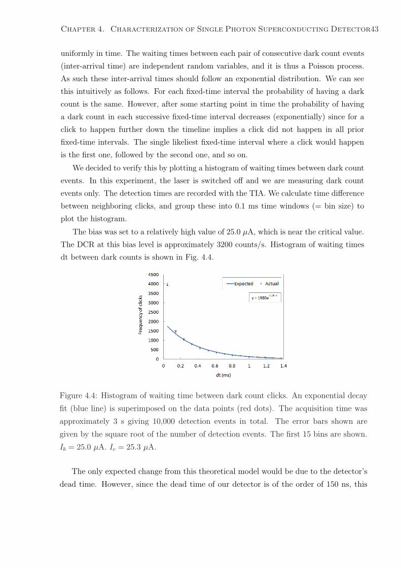
Chapter 4. Characterization of Single Photon Superconducting Detector43
uniformly in time. The waiting times between each pair of consecutive dark count events
(inter-arrival time) are independent random variables, and it is thus a Poisson process.
As such these inter-arrival times should follow an exponential distribution. We can see
this intuitively as follows. For each fixed-time interval the probability of having a dark
count is the same. However, after some starting point in time the probability of having
a dark count in each successive fixed-time interval decreases (exponentially) since for a
click to happen further down the timeline implies a click did not happen in all prior
fixed-time intervals. The single likeliest fixed-time interval where a click would happen
is the first one, followed by the second one, and so on.
We decided to verify this by plotting a histogram of waiting times between dark count
events. In this experiment, the laser is switched off and we are measuring dark count
events only. The detection times are recorded with the TIA. We calculate time difference
between neighboring clicks, and group these into 0.1 ms time windows (= bin size) to
plot the histogram.
The bias was set to a relatively high value of 25.0 µA, which is near the critical value.
The DCR at this bias level is approximately 3200 counts/s. Histogram of waiting times
dt between dark counts is shown in Fig. 4.4.
Figure 4.4: Histogram of waiting time between dark count clicks. An exponential decay
fit (blue line) is superimposed on the data points (red dots). The acquisition time was
approximately 3 s giving 10,000 detection events in total. The error bars shown are
given by the square root of the number of detection events. The first 15 bins are shown.
Ib = 25.0 µA. Ic = 25.3 µA.
The only expected change from this theoretical model would be due to the detector’s
dead time. However, since the dead time of our detector is of the order of 150 ns, this
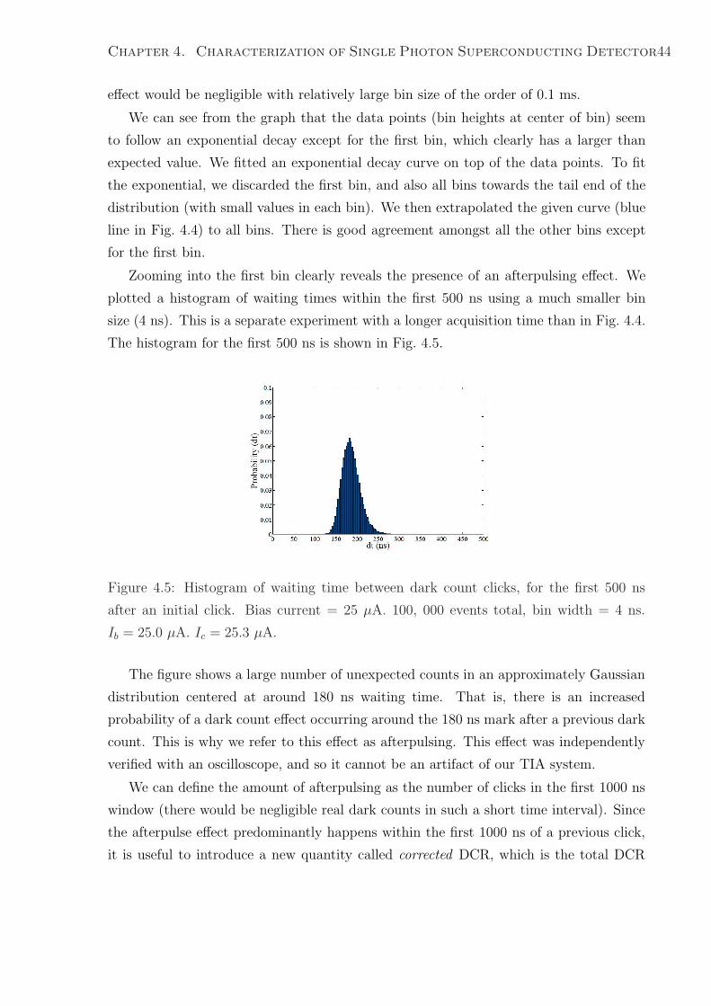
Chapter 4. Characterization of Single Photon Superconducting Detector44
effect would be negligible with relatively large bin size of the order of 0.1 ms.
We can see from the graph that the data points (bin heights at center of bin) seem
to follow an exponential decay except for the first bin, which clearly has a larger than
expected value. We fitted an exponential decay curve on top of the data points. To fit
the exponential, we discarded the first bin, and also all bins towards the tail end of the
distribution (with small values in each bin). We then extrapolated the given curve (blue
line in Fig. 4.4) to all bins. There is good agreement amongst all the other bins except
for the first bin.
Zooming into the first bin clearly reveals the presence of an afterpulsing effect. We
plotted a histogram of waiting times within the first 500 ns using a much smaller bin
size (4 ns). This is a separate experiment with a longer acquisition time than in Fig. 4.4.
The histogram for the first 500 ns is shown in Fig. 4.5.
Figure 4.5: Histogram of waiting time between dark count clicks, for the first 500 ns
after an initial click. Bias current = 25 µA. 100, 000 events total, bin width = 4 ns.
Ib = 25.0 µA. Ic = 25.3 µA.
The figure shows a large number of unexpected counts in an approximately Gaussian
distribution centered at around 180 ns waiting time. That is, there is an increased
probability of a dark count effect occurring around the 180 ns mark after a previous dark
count. This is why we refer to this effect as afterpulsing. This effect was independently
verified with an oscilloscope, and so it cannot be an artifact of our TIA system.
We can define the amount of afterpulsing as the number of clicks in the first 1000 ns
window (there would be negligible real dark counts in such a short time interval). Since
the afterpulse effect predominantly happens within the first 1000 ns of a previous click,
it is useful to introduce a new quantity called corrected DCR, which is the total DCR
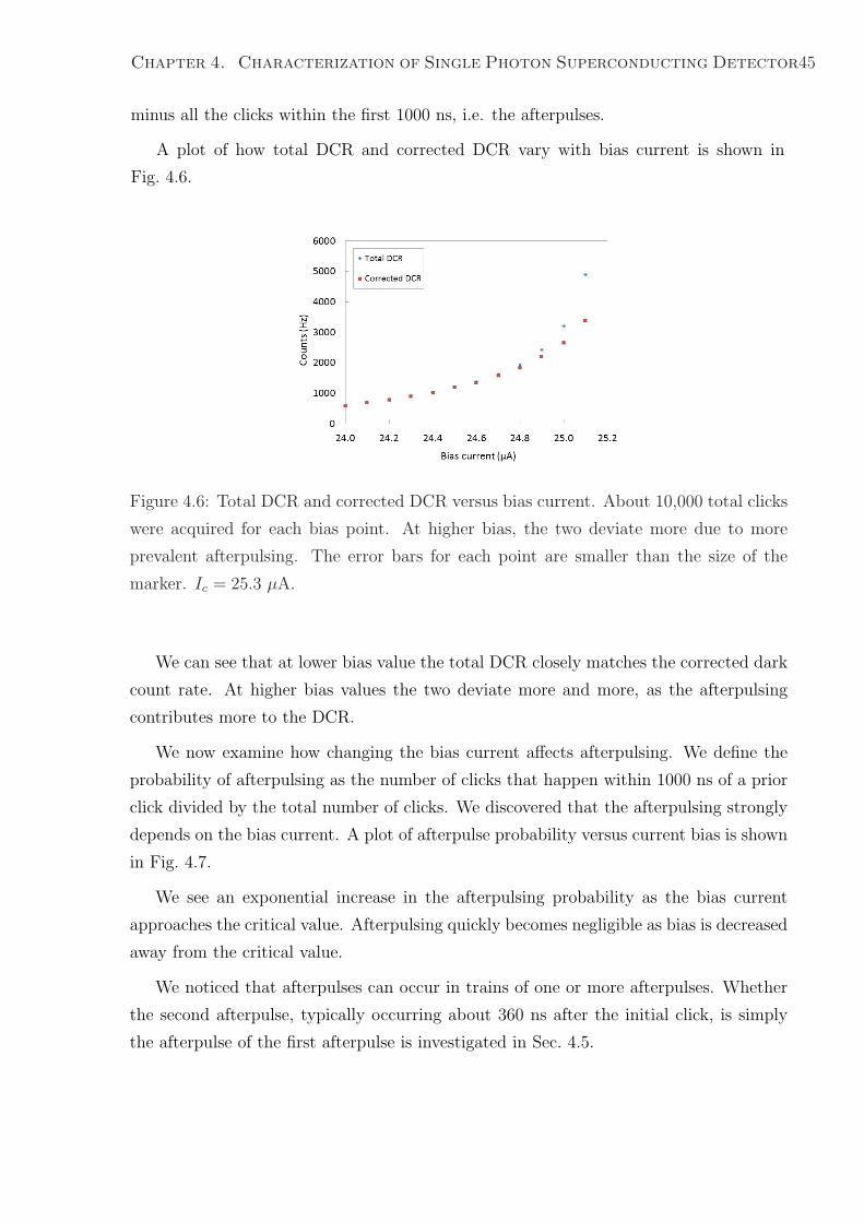
Chapter 4. Characterization of Single Photon Superconducting Detector45
minus all the clicks within the first 1000 ns, i.e. the afterpulses.
A plot of how total DCR and corrected DCR vary with bias current is shown in
Fig. 4.6.
Figure 4.6: Total DCR and corrected DCR versus bias current. About 10,000 total clicks
were acquired for each bias point. At higher bias, the two deviate more due to more
prevalent afterpulsing. The error bars for each point are smaller than the size of the
marker. Ic = 25.3 µA.
We can see that at lower bias value the total DCR closely matches the corrected dark
count rate. At higher bias values the two deviate more and more, as the afterpulsing
contributes more to the DCR.
We now examine how changing the bias current affects afterpulsing. We define the
probability of afterpulsing as the number of clicks that happen within 1000 ns of a prior
click divided by the total number of clicks. We discovered that the afterpulsing strongly
depends on the bias current. A plot of afterpulse probability versus current bias is shown
in Fig. 4.7.
We see an exponential increase in the afterpulsing probability as the bias current
approaches the critical value. Afterpulsing quickly becomes negligible as bias is decreased
away from the critical value.
We noticed that afterpulses can occur in trains of one or more afterpulses. Whether
the second afterpulse, typically occurring about 360 ns after the initial click, is simply
the afterpulse of the first afterpulse is investigated in Sec. 4.5.
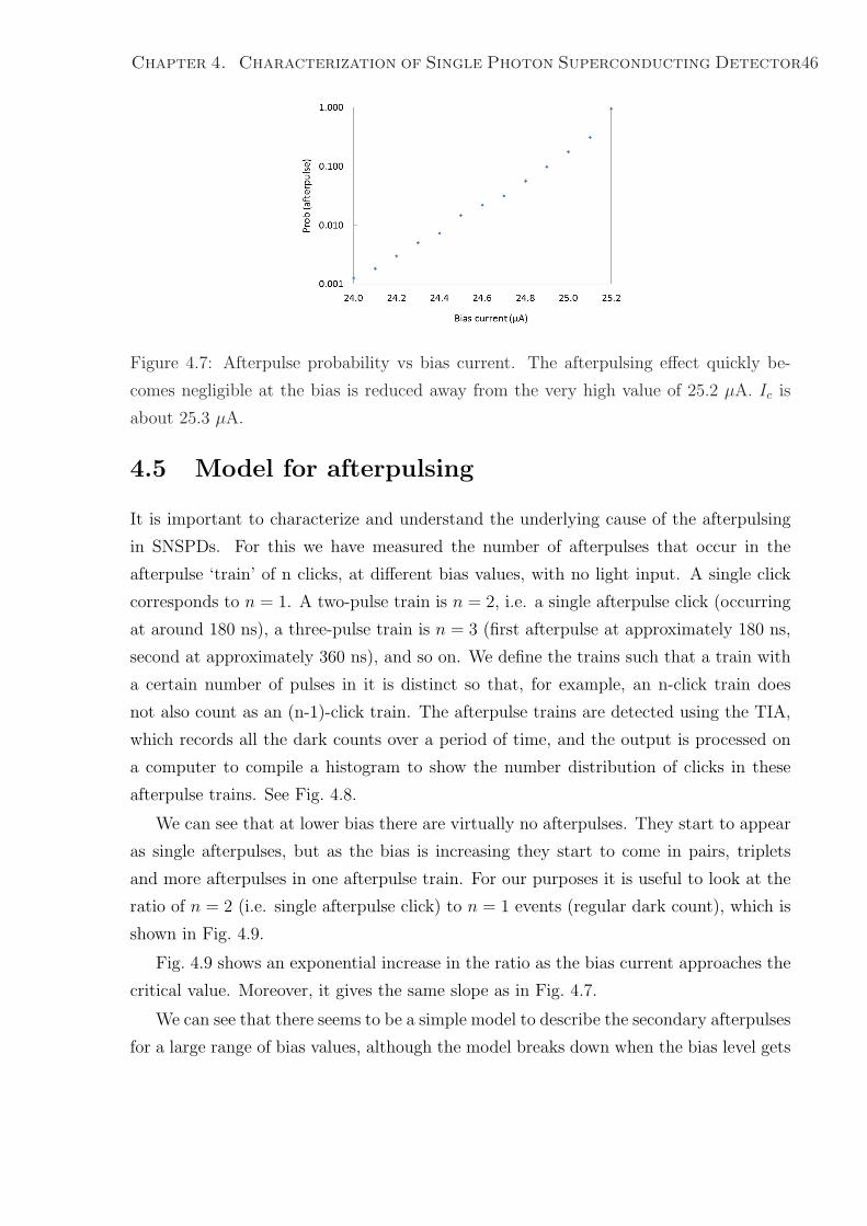
Chapter 4. Characterization of Single Photon Superconducting Detector46
Figure 4.7: Afterpulse probability vs bias current. The afterpulsing effect quickly be-
comes negligible at the bias is reduced away from the very high value of 25.2 µA. Ic is
about 25.3 µA.
4.5 Model for afterpulsing
It is important to characterize and understand the underlying cause of the afterpulsing
in SNSPDs. For this we have measured the number of afterpulses that occur in the
afterpulse ‘train’ of n clicks, at different bias values, with no light input. A single click
corresponds to n = 1. A two-pulse train is n = 2, i.e. a single afterpulse click (occurring
at around 180 ns), a three-pulse train is n = 3 (first afterpulse at approximately 180 ns,
second at approximately 360 ns), and so on. We define the trains such that a train with
a certain number of pulses in it is distinct so that, for example, an n-click train does
not also count as an (n-1)-click train. The afterpulse trains are detected using the TIA,
which records all the dark counts over a period of time, and the output is processed on
a computer to compile a histogram to show the number distribution of clicks in these
afterpulse trains. See Fig. 4.8.
We can see that at lower bias there are virtually no afterpulses. They start to appear
as single afterpulses, but as the bias is increasing they start to come in pairs, triplets
and more afterpulses in one afterpulse train. For our purposes it is useful to look at the
ratio of n = 2 (i.e. single afterpulse click) to n = 1 events (regular dark count), which is
shown in Fig. 4.9.
Fig. 4.9 shows an exponential increase in the ratio as the bias current approaches the
critical value. Moreover, it gives the same slope as in Fig. 4.7.
We can see that there seems to be a simple model to describe the secondary afterpulses
for a large range of bias values, although the model breaks down when the bias level gets
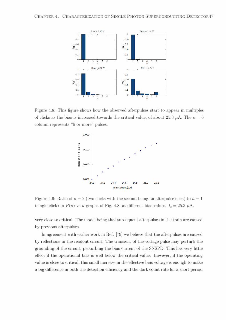
Chapter 4. Characterization of Single Photon Superconducting Detector47
Figure 4.8: This figure shows how the observed afterpulses start to appear in multiples
of clicks as the bias is increased towards the critical value, of about 25.3 µA. The n = 6
column represents “6 or more” pulses.
Figure 4.9: Ratio of n = 2 (two clicks with the second being an afterpulse click) to n = 1
(single click) in P (n) vs n graphs of Fig. 4.8, at different bias values. Ic = 25.3 µA.
very close to critical. The model being that subsequent afterpulses in the train are caused
by previous afterpulses.
In agreement with earlier work in Ref. [79] we believe that the afterpulses are caused
by reflections in the readout circuit. The transient of the voltage pulse may perturb the
grounding of the circuit, perturbing the bias current of the SNSPD. This has very little
effect if the operational bias is well below the critical value. However, if the operating
value is close to critical, this small increase in the effective bias voltage is enough to make
a big difference in both the detection efficiency and the dark count rate for a short period
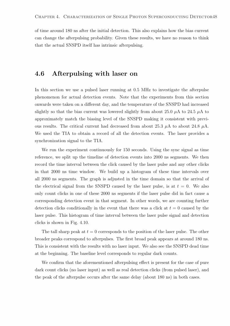
Chapter 4. Characterization of Single Photon Superconducting Detector48
of time around 180 ns after the initial detection. This also explains how the bias current
can change the afterpulsing probability. Given these results, we have no reason to think
that the actual SNSPD itself has intrinsic afterpulsing.
4.6 Afterpulsing with laser on
In this section we use a pulsed laser running at 0.5 MHz to investigate the afterpulse
phenomenon for actual detection events. Note that the experiments from this section
onwards were taken on a different day, and the temperature of the SNSPD had increased
slightly so that the bias current was lowered slightly from about 25.0 µA to 24.5 µA to
approximately match the biasing level of the SNSPD making it consistent with previ-
ous results. The critical current had decreased from about 25.3 µA to about 24.8 µA.
We used the TIA to obtain a record of all the detection events. The laser provides a
synchronization signal to the TIA.
We run the experiment continuously for 150 seconds. Using the sync signal as time
reference, we split up the timeline of detection events into 2000 ns segments. We then
record the time interval between the click caused by the laser pulse and any other clicks
in that 2000 ns time window. We build up a histogram of these time intervals over
all 2000 ns segments. The graph is adjusted in the time domain so that the arrival of
the electrical signal from the SNSPD caused by the laser pulse, is at t = 0. We also
only count clicks in one of these 2000 ns segments if the laser pulse did in fact cause a
corresponding detection event in that segment. In other words, we are counting further
detection clicks conditionally in the event that there was a click at t = 0 caused by the
laser pulse. This histogram of time interval between the laser pulse signal and detection
clicks is shown in Fig. 4.10.
The tall sharp peak at t = 0 corresponds to the position of the laser pulse. The other
broader peaks correspond to afterpulses. The first broad peak appears at around 180 ns.
This is consistent with the results with no laser input. We also see the SNSPD dead time
at the beginning. The baseline level corresponds to regular dark counts.
We confirm that the aforementioned afterpulsing effect is present for the case of pure
dark count clicks (no laser input) as well as real detection clicks (from pulsed laser), and
the peak of the afterpulse occurs after the same delay (about 180 ns) in both cases.
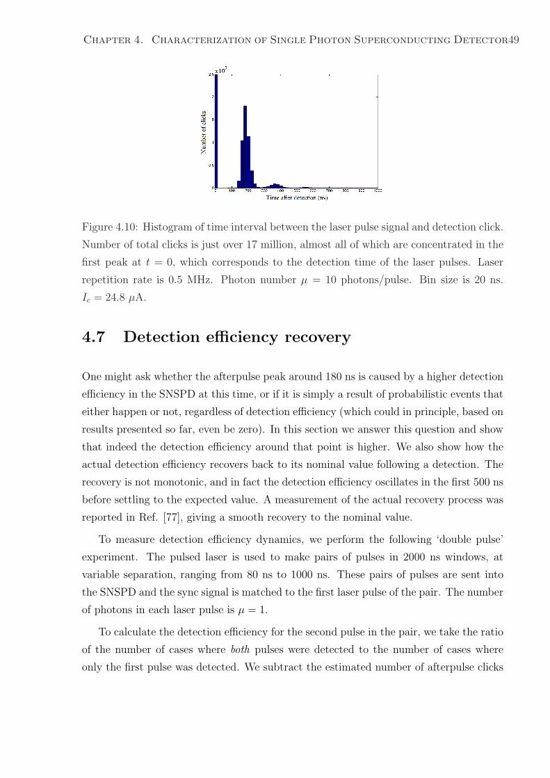
Chapter 4. Characterization of Single Photon Superconducting Detector49
Figure 4.10: Histogram of time interval between the laser pulse signal and detection click.
Number of total clicks is just over 17 million, almost all of which are concentrated in the
first peak at t = 0, which corresponds to the detection time of the laser pulses. Laser
repetition rate is 0.5 MHz. Photon number µ = 10 photons/pulse. Bin size is 20 ns.
Ic = 24.8 µA.
4.7 Detection efficiency recovery
One might ask whether the afterpulse peak around 180 ns is caused by a higher detection
efficiency in the SNSPD at this time, or if it is simply a result of probabilistic events that
either happen or not, regardless of detection efficiency (which could in principle, based on
results presented so far, even be zero). In this section we answer this question and show
that indeed the detection efficiency around that point is higher. We also show how the
actual detection efficiency recovers back to its nominal value following a detection. The
recovery is not monotonic, and in fact the detection efficiency oscillates in the first 500 ns
before settling to the expected value. A measurement of the actual recovery process was
reported in Ref. [77], giving a smooth recovery to the nominal value.
To measure detection efficiency dynamics, we perform the following ‘double pulse’
experiment. The pulsed laser is used to make pairs of pulses in 2000 ns windows, at
variable separation, ranging from 80 ns to 1000 ns. These pairs of pulses are sent into
the SNSPD and the sync signal is matched to the first laser pulse of the pair. The number
of photons in each laser pulse is µ = 1.
To calculate the detection efficiency for the second pulse in the pair, we take the ratio
of the number of cases where both pulses were detected to the number of cases where
only the first pulse was detected. We subtract the estimated number of afterpulse clicks
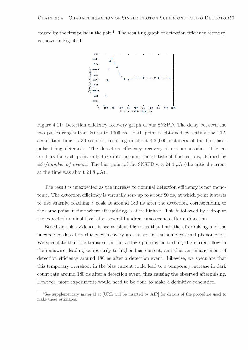
Chapter 4. Characterization of Single Photon Superconducting Detector50
caused by the first pulse in the pair 4. The resulting graph of detection efficiency recovery
is shown in Fig. 4.11.
Figure 4.11: Detection efficiency recovery graph of our SNSPD. The delay between the
two pulses ranges from 80 ns to 1000 ns. Each point is obtained by setting the TIA
acquisition time to 30 seconds, resulting in about 400,000 instances of the first laser
pulse being detected. The detection efficiency recovery is not monotonic. The er-
ror bars for each point only take into account the statistical fluctuations, defined by
±3√
number of events. The bias point of the SNSPD was 24.4 µA (the critical current
at the time was about 24.8 µA).
The result is unexpected as the increase to nominal detection efficiency is not mono-
tonic. The detection efficiency is virtually zero up to about 80 ns, at which point it starts
to rise sharply, reaching a peak at around 180 ns after the detection, corresponding to
the same point in time where afterpulsing is at its highest. This is followed by a drop to
the expected nominal level after several hundred nanoseconds after a detection.
Based on this evidence, it seems plausible to us that both the afterpulsing and the
unexpected detection efficiency recovery are caused by the same external phenomenon.
We speculate that the transient in the voltage pulse is perturbing the current flow in
the nanowire, leading temporarily to higher bias current, and thus an enhancement of
detection efficiency around 180 ns after a detection event. Likewise, we speculate that
this temporary overshoot in the bias current could lead to a temporary increase in dark
count rate around 180 ns after a detection event, thus causing the observed afterpulsing.
However, more experiments would need to be done to make a definitive conclusion.
4See supplementary material at [URL will be inserted by AIP] for details of the procedure used tomake these estimates.
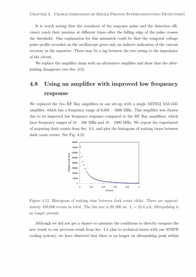
Chapter 4. Characterization of Single Photon Superconducting Detector51
It is worth noting that the overshoot of the response pulse and the detection effi-
ciency reach their maxima at different times after the falling edge of the pulse crosses
the threshold. One explanation for this mismatch could be that the temporal voltage
pulse profile recorded on the oscilloscope gives only an indirect indication of the current
recovery in the nanowire. There may be a lag between the two owing to the impedance
of the circuit.
We replace the amplifier chain with an alternative amplifier and show that the after-
pulsing disappears (see Sec. 4.8).
4.8 Using an amplifier with improved low frequency
response
We replaced the two RF Bay amplifiers in our set-up with a single MITEQ AM-1431
amplifier, which has a frequency range of 0.001 – 1000 MHz. This amplifier was chosen
due to its improved low frequency response compared to the RF Bay amplifiers, which
have frequency ranges of 10 – 580 MHz and 10 – 1000 MHz. We repeat the experiment
of acquiring dark counts from Sec. 4.4, and plot the histogram of waiting times between
dark count events. See Fig. 4.12.
Figure 4.12: Histogram of waiting time between dark count clicks. There are approxi-
mately 450,000 events in total. The bin size is 20, 000 ns. Ic = 24.8 µA. Afterpulsing is
no longer present.
Although we did not get a chance to optimize the conditions to directly compare the
new result to our previous result from Sec. 4.4 (due to technical issues with our SNSPD
cooling system), we have observed that there is no longer an afterpulsing peak within
Chapter 4. Characterization of Single Photon Superconducting Detector52
the first 500 ns after a dark count, and as such, there is no longer an abnormally high
number of clicks in the first bin as we can see from Fig. 4.12.
We speculate that the poor low frequency response of the RF Bay LNA-580 and LNA-
1000 amplifiers used caused an oscillation in the output voltage pulse during recovery,
leading to the afterpulsing effect, as suggested in Ref. [79].
4.9 Summary and Conclusions
The contributions of this thesis can be summarized in terms of three main parts. First,
we have performed the first experimental study of the time-domain distribution of dark
counts in an SNSPD (i.e. the case with no laser input), showing for the first time, an
afterpulsing effect. Second, we have also performed a longer time domain measurement
of the afterpulsing effect (1000 ns) with laser input. Third, we have measured the ac-
tual recovery graph of the detection efficiency and found that the recovery occurs in an
unexpected manner. Specifically, we found that the detection efficiency after a detection
event starts from zero, rises and actually overshoots before returning to its normal value.
The afterpulsing, dark count and detection efficiency enhancement during the recov-
ery of the SNSPD show similar dynamics and are all most likely to occur around 180 ns
following a detection event (the exact figure depends on the biasing current). We specu-
late that all three of these effects arise due to a perturbation in the bias current through
the nanowire. This is caused by the poor low frequency response of the RF Bay LNA-
580 and LNA-1000 amplifiers used, causing an oscillation in the output voltage pulse
during recovery, as suggested in Ref. [79]. It thus appears that the afterpulsing effect is
not intrinsic to the SNSPD itself. We confirmed experimentally that afterpulsing does
indeed disappear when we replace the aforementioned RF Bay amplifiers with a MITEQ
AM-1431 amplifier which has a much better low frequency response.
We also want to emphasize the significance of afterpulsing and the recovery profile
in QKD applications. One unwanted effect would be if someone chose to operate the
system at around 5 MHz repetition rate (corresponding to about 200 ns between pulses),
and thereby significantly increasing the effective dark count rate, and hence lowering the
secure key rate. It is also natural to ask whether such a recovery profile can cause any
security concern for a QKD system. First of all, it was shown in [90] that the proven
secure key rate is much lower, in view of detection efficiency mismatch. Second, if Eve
always sends signals separated by 180 ns to Bob, then she can gain side information
Chapter 4. Characterization of Single Photon Superconducting Detector53
about the sifted key.
One should be careful about the electronics used in a QKD system as electronics may
give false detection signals and afterpulsing effects that may severely undermine security
and/or performance of a QKD system. However, even if there is an exploitable loophole
due to afterpulsing, the newly developed MDI-QKD [91] can close all such loopholes in
the detection system, including unidentified ones.
Chapter 5
Conclusion and outlook
This chapter concludes the findings of the thesis, and provides a perspective for the
future.
5.1 Conclusion:
There are two main points in this thesis: the importance of optimization in the design
of protocols and the importance of characterization for new devices in Quantum Key
Distribution (QKD).
5.1.1 Protocol Optimization:
The goal of optimization is not to merely save computational time and resources; these
savings are usually only a by-product of a superior optimization algorithm. Rather, the
goal of optimization is to probe the extreme possibilities of a given protocol. For example,
in our optimization, the local search algorithm can improve the key rate by 200 %.
In this thesis, I have presented a framework for the optimization of protocols by
showing:
• recognition of a convex topology can save efforts in optimization.
• identification of controllable parameters must be done to extract the most influential
parameters while ignoring others with only spurious and negligible effects.
• optimization algorithm depends on the topology and the parameters,
54
Chapter 5. Conclusion and outlook 55
5.1.2 Detector Characterization:
No matter which type of the device is, and what its physical mechanism is , characteri-
zation of the device must be done prior to its use. Such tomographic processes not only
make subsequent experiment predictable, but also isolate out many faulty hypotheses of
the experiment without expensive equipment renting.
In this thesis, I have presented one aspect of the characterization, namely the origin
and elimination of the afterpulse phenomenon. Following the approach in this thesis,
other researchers can predict the presence of the afterpulse, and eliminate it if it is
undesirable.
5.1.3 General Conclusion:
Aside from the prominent promise of a 200 % increase in the key rate, the proposed
methodologies on the optimization of parameters and on the characterization of devices
allow any QKD researchers to save efforts on the selection of parameters and on the
probing of new devices.
The insights gained in the optimization can potentially compensate technological
deficiency such as the lack of true SPDs. Our local search algorithm makes the MDI-QKD
protocols more tolerant to photon loss, and the increased key rate allows experimentalists
a larger design space to use less expensive devices. The results on how to choose the
number of decoy states fill the un-answered question ofhow many of decoy states make a
superior protocol.
Our works on the characterization of SNSPD can be extended and generalized to
an understanding of novel devices. Our approaches in both the time domain and the
frequency domain can easily be adapted as a tomographic process for general devices.
Although the time and frequency behaviour may differ, the interpretations from the
characterization will aid researchers to better cope with the non-idealities of the devices
and squeeze out the most from the device.
To put our work in a larger perspective, this thesis brings to the QKD community
a step further into closing the gap between theory and practice. Finally, this thesis
impacts both industry and academia by advancing the QKD protocols a step further
from laboratory experiments to viable commercial products. Our results may persuade
the industry that QKD does not solely rely on un-realistic technological assumptions.
The advent of commercial QKD products may be influenced by our work.
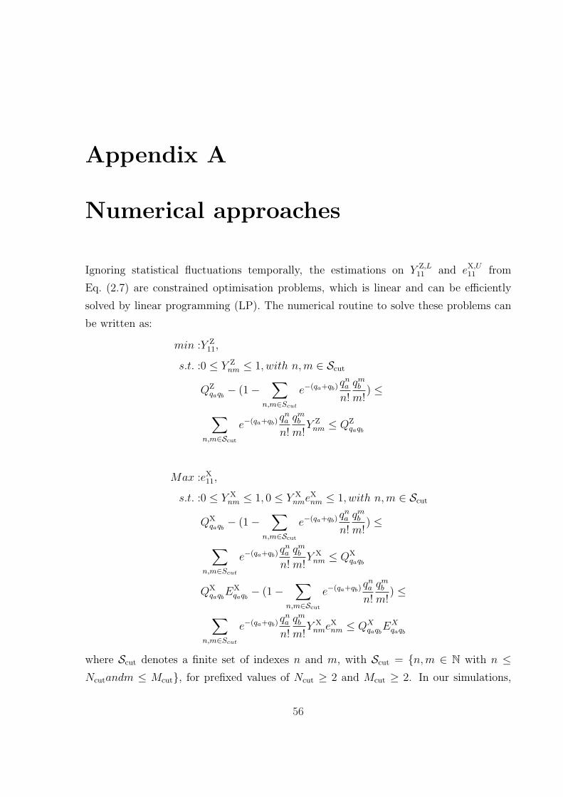
Appendix A
Numerical approaches
Ignoring statistical fluctuations temporally, the estimations on Y Z,L11 and eX,U
11 from
Eq. (2.7) are constrained optimisation problems, which is linear and can be efficiently
solved by linear programming (LP). The numerical routine to solve these problems can
be written as:
min :Y Z11,
s.t. :0 ≤ Y Znm ≤ 1, with n, m ∈ Scut
QZqaqb
− (1−∑
n,m∈Scut
e−(qa+qb)qna
n!
qmb
m!) ≤
∑n,m∈Scut
e−(qa+qb)qna
n!
qmb
m!Y Z
nm ≤ QZqaqb
Max :eX11,
s.t. :0 ≤ Y Xnm ≤ 1, 0 ≤ Y X
nmeXnm ≤ 1, with n, m ∈ Scut
QXqaqb
− (1−∑
n,m∈Scut
e−(qa+qb)qna
n!
qmb
m!) ≤
∑n,m∈Scut
e−(qa+qb)qna
n!
qmb
m!Y X
nm ≤ QXqaqb
QXqaqb
EXqaqb
− (1−∑
n,m∈Scut
e−(qa+qb)qna
n!
qmb
m!) ≤
∑n,m∈Scut
e−(qa+qb)qna
n!
qmb
m!Y X
nmeXnm ≤ QX
qaqbEX
qaqb
where Scut denotes a finite set of indexes n and m, with Scut = n,m ∈ N with n ≤Ncutandm ≤ Mcut, for prefixed values of Ncut ≥ 2 and Mcut ≥ 2. In our simulations,
56
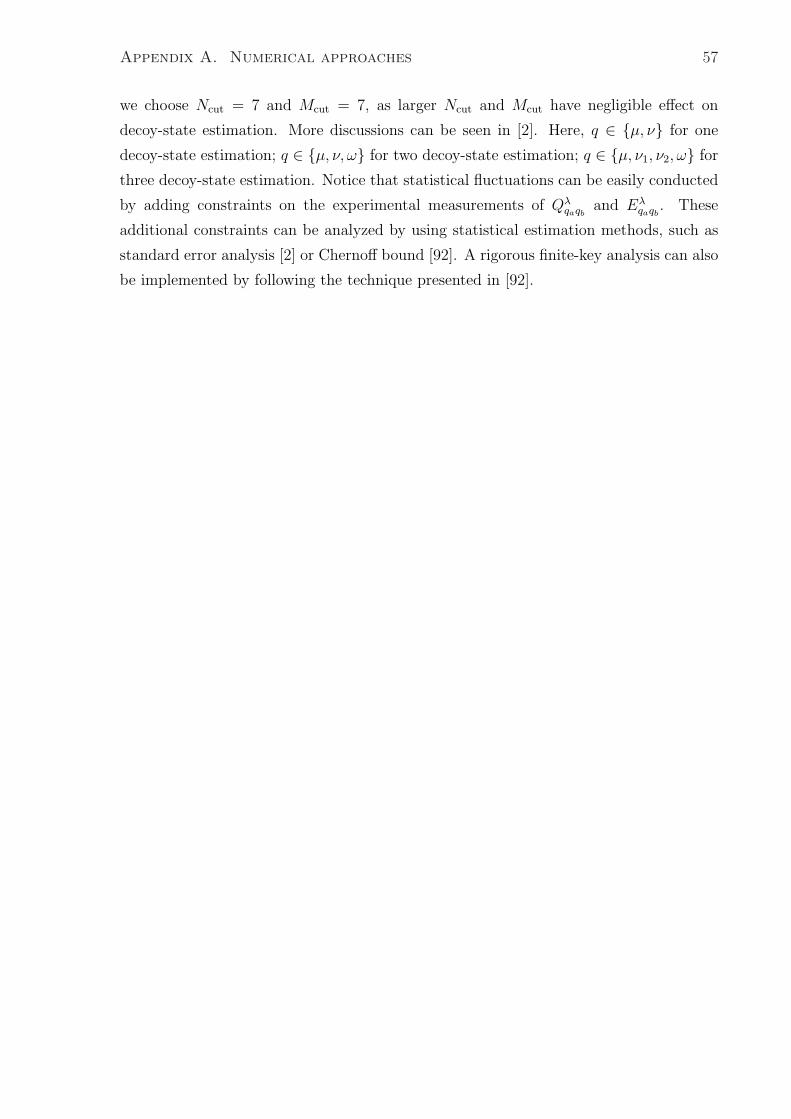
Appendix A. Numerical approaches 57
we choose Ncut = 7 and Mcut = 7, as larger Ncut and Mcut have negligible effect on
decoy-state estimation. More discussions can be seen in [2]. Here, q ∈ µ, ν for one
decoy-state estimation; q ∈ µ, ν, ω for two decoy-state estimation; q ∈ µ, ν1, ν2, ω for
three decoy-state estimation. Notice that statistical fluctuations can be easily conducted
by adding constraints on the experimental measurements of Qλqaqb
and Eλqaqb
. These
additional constraints can be analyzed by using statistical estimation methods, such as
standard error analysis [2] or Chernoff bound [92]. A rigorous finite-key analysis can also
be implemented by following the technique presented in [92].
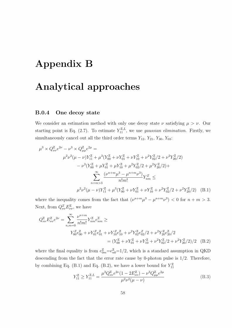
Appendix B
Analytical approaches
B.0.4 One decoy state
We consider an estimation method with only one decoy state ν satisfying µ > ν. Our
starting point is Eq. (2.7). To estimate Y Z,L11 , we use gaussian elimination. Firstly, we
simultaneously cancel out all the third order terms Y12, Y21, Y30, Y03:
µ3 ×QZννe
2ν − ν3 ×QZµµe
2µ =
µ2ν2(µ− ν)Y Z11 + µ3(Y Z
00 + νY Z01 + νY Z
10 + ν2Y Z02/2 + ν2Y Z
20/2)
− ν3(Y Z00 + µY Z
01 + µY Z10 + µ2Y Z
02/2 + µ2Y Z20/2)+
∞∑n+m>3
(νn+mµ3 − µn+mν3)
n!m!Y Z
nm ≤
µ2ν2(µ− ν)Y Z11 + µ3(Y Z
00 + νY Z01 + νY Z
10 + ν2Y Z02/2 + ν2Y Z
20/2) (B.1)
where the inequality comes from the fact that (νn+mµ3 − µn+mν3) < 0 for n + m > 3.
Next, from QZννE
Zνν , we have
QZννE
Zννe
2ν =∞∑
n,m=0
νn+m
n!m!Y Z
nmeZnm ≥
Y Z00e
Z00 + νY Z
01eZ01 + νY Z
10eZ10 + ν2Y Z
02eZ02/2 + ν2Y Z
20eZ20/2
= (Y Z00 + νY Z
01 + νY Z10 + ν2Y Z
02/2 + ν2Y Z20/2)/2 (B.2)
where the final equality is from eZ0m=eZ
n0=1/2, which is a standard assumption in QKD
descending from the fact that the error rate cause by 0-photon pulse is 1/2. Therefore,
by combining Eq. (B.1) and Eq. (B.2), we have a lower bound for Y Z11
Y Z11 ≥ Y Z,L
11 =µ3QZ
ννe2ν(1− 2EZ
νν)− ν3QZµµe
2µ
µ2ν2(µ− ν)(B.3)
58
Appendix B. Analytical approaches 59
To estimate eX,U11 , we use the same method as [45, 92] and obtain an upper bound for
eX11
eX11 ≤ eX,U
11 =1
(µ− ν)2Y X,L11
×
(e2µQXµµE
Xµµ + e2νQX
ννEXνν − eµ+νQX
µνEXµν − eν+µQX
νµEXνµ) (B.4)
B.0.5 Two decoy states
We consider an estimation method with two decoy states ν, ω satisfying µ > ν > ω ≥ 0.
We have the lower bound Y Z,L11 and the upper bound eX,U
11 [45, 92]
Y Z,L11 =
1
(µ− ω)2(ν − ω)2(µ− ν)×
[(µ2 − ω2)(µ− ω)(QZννe
2ν + QZωωe2ω −QZ
νωeν+ω −QZωνe
ω+ν)
− (ν2 − ω2)(ν − ω)(QZµµe
2µ + QZωωe2ω −QZ
µωeµ+ω −QZωµe
ω+µ)], (B.5)
eX,U11 =
1
(ν − ω)2Y X,L11
×
[e2νQXννE
Xνν + e2ωQX
ωωEXωω − eν+ωQX
νωEXνω − eω+νQX
ωνEXων ]. (B.6)
Appendix C
Simulation in Simulink
The Simulink model presented in Fig C.1 consists of 3 main parts: Source, Circuit
and Read-out parts.
The source part:
• Signal 1 and Signal 2: The switchings from superconducting state to normal state
and subsequent restorations are modeled by combination of “signal1 + switch” and
“signal 2 + switch1”. The two switches are complementary in the sense that there
is always one switch closed and the other switch open. In Simulink, a switch must
be controled by a signal source.
• Signal to Physical Signal Converter (S-PS): Signals are most conveniently generate
by abstract source rather than physical. Hence, S-PS converter are needed as a
interface between the abstract signal source and Realistic voltage/current signals.
• Solver Configuration: Each circuit must have a configuratoin block to set the meta-
parameters such as simulation duration and minimum simulation time step, etc...
The circuit models:
• Resistor + Switch: this combination models the normal state
• Switch 1: this component alone models the superconducting state
• Electrical Reference: for each configuration blocks there must a corresponding gnd
block.
60
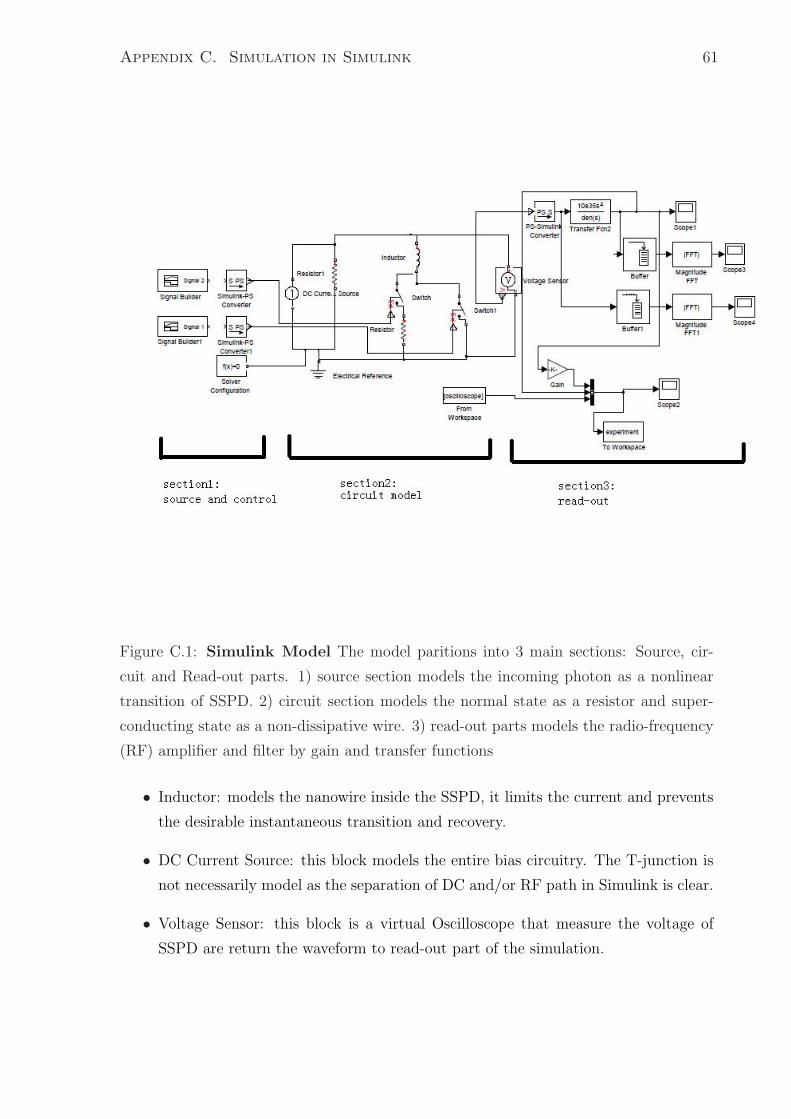
Appendix C. Simulation in Simulink 61
Figure C.1: Simulink Model The model paritions into 3 main sections: Source, cir-
cuit and Read-out parts. 1) source section models the incoming photon as a nonlinear
transition of SSPD. 2) circuit section models the normal state as a resistor and super-
conducting state as a non-dissipative wire. 3) read-out parts models the radio-frequency
(RF) amplifier and filter by gain and transfer functions
• Inductor: models the nanowire inside the SSPD, it limits the current and prevents
the desirable instantaneous transition and recovery.
• DC Current Source: this block models the entire bias circuitry. The T-junction is
not necessarily model as the separation of DC and/or RF path in Simulink is clear.
• Voltage Sensor: this block is a virtual Oscilloscope that measure the voltage of
SSPD are return the waveform to read-out part of the simulation.

Appendix C. Simulation in Simulink 62
The read-out models:
• Physical Signal - Signal Converter (PS-S): this self-explanatory block provide the
dual functionality of S-PS converter at the source side
• Transfer Fcn2: this blocks models the filter bandwidth limitation of the RF-
amplifier chain in the experiment. This filter is designed as a 3rd order ButterWorth
Filter.
• Gain: this block models the gain and inverting properties of the amplifier chain,
the exactly value is from the product specification of the amplifier.
• From Workspace + To workspace: this combination is not physical, but make it
convenient to load and writeback a waveform to Matlab environment. Matlab
environment handles complex processing easier than Simulink environment.
• Scope’s: these blocks is virtual oscilloscope that display time domain waveform of
the simulated output
• Buffer+ Magnitude FFT + scope: this combination measure frequency domain
waveform of the simulated output before AND after the amplifier chains
This Simulink model captures the essential detail of the SSPD and successful simu-
lated results and the matched experimental result are presented in Section 4.5
Bibliography
[1] R. Ursin, F. Tiefenbacher, T. Schmitt-Manderbach, H. Weier, T. Scheidl, M. Linden-
thal, B. Blauensteiner, T. Jennewein, J. Perdigues, P. Trojek, et al., “Entanglement-
based quantum communication over 144 km,” Nature physics, vol. 3, no. 7, pp. 481–
486, 2007.
[2] X. Ma, C.-H. F. Fung, and M. Razavi, “Statistical fluctuation analysis for
measurement-device-independent quantum key distribution,” Physical Review A,
vol. 86, no. 5, p. 052305, 2012.
[3] S.-H. Sun, M. Gao, C.-Y. Li, and L.-M. Liang, “Practical decoy-state measurement-
device-independent quantum key distribution,” Physical Review A, vol. 87, no. 5,
p. 052329, 2013.
[4] Y. Zhao, B. Qi, X. Ma, H.-K. Lo, and L. Qian, “Experimental quantum key distri-
bution with decoy states,” Physical review letters, vol. 96, no. 7, p. 070502, 2006.
[5] D. Rosenberg, J. W. Harrington, P. R. Rice, P. A. Hiskett, C. G. Peterson, R. J.
Hughes, A. E. Lita, S. W. Nam, and J. E. Nordholt, “Long-distance decoy-state
quantum key distribution in optical fiber,” Physical review letters, vol. 98, no. 1,
p. 010503, 2007.
[6] A. Dixon, Z. Yuan, J. Dynes, A. Sharpe, and A. Shields, “Gigahertz decoy quantum
key distribution with 1 mbit/s secure key rate,” Optics express, vol. 16, no. 23,
pp. 18790–18979, 2008.
[7] M. Lucamarini, K. Patel, J. Dynes, B. Frohlich, A. Sharpe, A. Dixon, Z. Yuan,
R. Penty, and A. Shields, “Efficient decoy-state quantum key distribution with quan-
tified security,” Optics express, vol. 21, no. 21, pp. 24550–24565, 2013.
63
Bibliography 64
[8] Z. Liao, Experimental Realization of Decoy State Polarization Encoding
Measurement-Device-Independent Quantum Key Distribution. PhD thesis, Univer-
sity of Toronto, 2013.
[9] Z.-W. Yu, Y.-H. Zhou, and X.-B. Wang, “Generalized three-intensity decoy state
method for measurement device independent quantum key distribution,” arXiv
preprint arXiv:1309.5886, 2013.
[10] C. M. Natarajan, M. G. Tanner, and R. H. Hadfield, “Superconducting nanowire
single-photon detectors: physics and applications,” Superconductor science and tech-
nology, vol. 25, no. 6, p. 063001, 2012.
[11] R. L. Rivest, A. Shamir, and L. Adleman, “A method for obtaining digital signatures
and public-key cryptosystems,” Communications of the ACM, vol. 21, no. 2, pp. 120–
126, 1978.
[12] G. S. Vernam, “Cipher printing telegraph systems: For secret wire and radio tele-
graphic communications,” AIEE, Journal of the, vol. 45, no. 2, pp. 109–115, 1926.
[13] C. E. Shannon, “Communication theory of secrecy systems*,” Bell system technical
journal, vol. 28, no. 4, pp. 656–715, 1949.
[14] D. Mayers, “Unconditional security in quantum cryptography,” Journal of the ACM
(JACM), vol. 48, no. 3, pp. 351–406, 2001.
[15] H.-K. Lo and H. F. Chau, “Unconditional security of quantum key distribution over
arbitrarily long distances,” Science, vol. 283, no. 5410, pp. 2050–2056, 1999.
[16] P. W. Shor and J. Preskill, “Simple proof of security of the bb84 quantum key
distribution protocol,” Physical Review Letters, vol. 85, no. 2, p. 441, 2000.
[17] S. Wiesner, “Conjugate coding,” ACM Sigact News, vol. 15, no. 1, pp. 78–88, 1983.
[18] C. H. Bennett, G. Brassard, et al., “Quantum cryptography: Public key distribution
and coin tossing,” in Proceedings of IEEE International Conference on Computers,
Systems and Signal Processing, vol. 175, p. 8, New York, 1984.
[19] A. K. Ekert, “Quantum cryptography based on bell’s theorem,” Physical review
letters, vol. 67, no. 6, pp. 661–663, 1991.
Bibliography 65
[20] W. K. Wootters and W. H. Zurek, “A single quantum cannot be cloned,” Nature,
vol. 299, no. 5886, pp. 802–803, 1982.
[21] D. Dieks, “Communication by epr devices,” Physics Letters A, vol. 92, no. 6, pp. 271–
272, 1982.
[22] A. Mirza and F. Petruccione, “Realizing long-term quantum cryptography,” JOSA
B, vol. 27, no. 6, pp. A185–A188, 2010.
[23] T.-Y. Chen, J. Wang, H. Liang, W.-Y. Liu, Y. Liu, X. Jiang, Y. Wang, X. Wan, W.-
Q. Cai, L. Ju, et al., “Metropolitan all-pass and inter-city quantum communication
network,” Optics express, vol. 18, no. 26, pp. 27217–27225, 2010.
[24] M. Sasaki, M. Fujiwara, H. Ishizuka, W. Klaus, K. Wakui, M. Takeoka, S. Miki,
T. Yamashita, Z. Wang, A. Tanaka, et al., “Field test of quantum key distribution
in the tokyo qkd network,” Optics Express, vol. 19, no. 11, pp. 10387–10409, 2011.
[25] B. Huttner, N. Imoto, N. Gisin, and T. Mor, “Quantum cryptography with coherent
states,” Physical Review A, vol. 51, no. 3, p. 1863, 1995.
[26] N. Lutkenhaus and M. Jahma, “Quantum key distribution with realistic states:
photon-number statistics in the photon-number splitting attack,” New Journal of
Physics, vol. 4, no. 1, p. 44, 2002.
[27] D. Gottesman, H.-K. Lo, N. Lutkenhaus, and J. Preskill, “Security of quantum key
distribution with imperfect devices,” arXiv preprint quant-ph/0212066, 2002.
[28] W.-Y. Hwang, “Quantum key distribution with high loss: Toward global secure
communication,” Physical Review Letters, vol. 91, no. 5, p. 057901, 2003.
[29] H.-K. Lo, X. Ma, and K. Chen, “Decoy state quantum key distribution,” Physical
Review Letters, vol. 94, no. 23, p. 230504, 2005.
[30] X.-B. Wang, “Beating the photon-number-splitting attack in practical quantum
cryptography,” Physical review letters, vol. 94, no. 23, p. 230503, 2005.
[31] B. Qi, C.-H. F. Fung, H.-K. Lo, and X. Ma, “Time-shift attack in practical quantum
cryptosystems,” arXiv preprint quant-ph/0512080, 2005.

Bibliography 66
[32] Y. Zhao, C.-H. F. Fung, B. Qi, C. Chen, and H.-K. Lo, “Quantum hacking:
Experimental demonstration of time-shift attack against practical quantum-key-
distribution systems,” Physical Review A, vol. 78, no. 4, p. 042333, 2008.
[33] L. Lydersen, C. Wiechers, C. Wittmann, D. Elser, J. Skaar, and V. Makarov, “Hack-
ing commercial quantum cryptography systems by tailored bright illumination,” Na-
ture photonics, vol. 4, no. 10, pp. 686–689, 2010.
[34] F. Xu, B. Qi, and H.-K. Lo, “Experimental demonstration of phase-remapping attack
in a practical quantum key distribution system,” New Journal of Physics, vol. 12,
no. 11, p. 113026, 2010.
[35] A. Acin, N. Brunner, N. Gisin, S. Massar, S. Pironio, and V. Scarani, “Device-
independent security of quantum cryptography against collective attacks,” Physical
Review Letters, vol. 98, no. 23, p. 230501, 2007.
[36] N. Gisin, S. Pironio, and N. Sangouard, “Proposal for implementing device-
independent quantum key distribution based on a heralded qubit amplifier,” Physical
review letters, vol. 105, no. 7, p. 070501, 2010.
[37] H.-K. Lo, M. Curty, and B. Qi, “Measurement-device-independent quantum key
distribution,” Physical review letters, vol. 108, no. 13, p. 130503, 2012.
[38] K. Tamaki, H.-K. Lo, C.-H. F. Fung, and B. Qi, “Phase encoding schemes for
measurement-device-independent quantum key distribution with basis-dependent
flaw,” Physical Review A, vol. 85, no. 4, p. 042307, 2012.
[39] A. Rubenok, J. A. Slater, P. Chan, I. Lucio-Martinez, and W. Tittel, “Real-world
two-photon interference and proof-of-principle quantum key distribution immune to
detector attacks,” Physical review letters, vol. 111, no. 13, p. 130501, 2013.
[40] Y. Liu, T.-Y. Chen, L.-J. Wang, H. Liang, G.-L. Shentu, J. Wang, K. Cui, H.-L. Yin,
N.-L. Liu, L. Li, et al., “Experimental measurement-device-independent quantum
key distribution,” Physical review letters, vol. 111, no. 13, p. 130502, 2013.
[41] L. Masanes, S. Pironio, and A. Acın, “Secure device-independent quantum key dis-
tribution with causally independent measurement devices,” Nature communications,
vol. 2, p. 238, 2011.
Bibliography 67
[42] Z. Tang, Z. Liao, F. Xu, B. Qi, L. Qian, and H.-K. Lo, “Experimental demonstra-
tion of polarization encoding measurement-device-independent quantum key distri-
bution,” Physical Review Letters, vol. 112, no. 19, p. 190503, 2014.
[43] Y.-L. Tang, H.-L. Yin, S.-J. Chen, Y. Liu, W.-J. Zhang, X. Jiang, L. Zhang, J. Wang,
L.-X. You, J.-Y. Guan, et al., “Measurement-device-independent quantum key dis-
tribution over 200 km,” arXiv preprint arXiv:1407.8012, 2014.
[44] Y.-L. Tang, H.-L. Yin, S.-J. Chen, Y. Liu, W.-J. Zhang, X. Jiang, L. Zhang, J. Wang,
L.-X. You, J.-Y. Guan, et al., “Field test of measurement-device-independent quan-
tum key distribution,” arXiv preprint arXiv:1408.2330, 2014.
[45] F. Xu, M. Curty, B. Qi, and H.-K. Lo, “Practical aspects of measurement-device-
independent quantum key distribution,” New Journal of Physics, vol. 15, no. 11,
p. 113007, 2013.
[46] X.-B. Wang, “Three-intensity decoy-state method for device-independent quantum
key distribution with basis-dependent errors,”
[47] M. Eisaman, J. Fan, A. Migdall, and S. Polyakov, “Invited review article: Single-
photon sources and detectors,” Review of scientific instruments, vol. 82, no. 7,
p. 071101, 2011.
[48] S. Cova, M. Ghioni, A. Lotito, I. Rech, and F. Zappa, “Evolution and prospects for
single-photon avalanche diodes and quenching circuits,” Journal of Modern Optics,
vol. 51, no. 9-10, pp. 1267–1288, 2004.
[49] G. GolTsman, O. Okunev, G. Chulkova, A. Lipatov, A. Semenov, K. Smirnov,
B. Voronov, A. Dzardanov, C. Williams, and R. Sobolewski, “Picosecond super-
conducting single-photon optical detector,” Applied Physics Letters, vol. 79, no. 6,
pp. 705–707, 2001.
[50] F. Xu, H. Xu, and H.-K. Lo, “Protocol choice and parameter optimization in decoy-
state measurement-device-independent quantum key distribution,” Physical Review
A, vol. 89, no. 5, p. 052333, 2014.
[51] V. Burenkov, H. Xu, B. Qi, R. H. Hadfield, and H.-K. Lo, “Investigations of after-
pulsing and detection efficiency recovery in superconducting nanowire single-photon
detectors,” Journal of Applied Physics, vol. 113, no. 21, p. 213102, 2013.
Bibliography 68
[52] J. J. Sakurai and S. F. Tuan, Modern quantum mechanics, vol. 1. Addison-Wesley
Reading, Massachusetts, 1985.
[53] Q. Wang, W. Chen, G. Xavier, M. Swillo, T. Zhang, S. Sauge, M. Tengner, Z.-F.
Han, G.-C. Guo, and A. Karlsson, “Experimental decoy-state quantum key distribu-
tion with a sub-poissionian heralded single-photon source,” Physical review letters,
vol. 100, no. 9, p. 090501, 2008.
[54] V. Scarani, H. Bechmann-Pasquinucci, N. J. Cerf, M. Dusek, N. Lutkenhaus, and
M. Peev, “The security of practical quantum key distribution,” Reviews of Modern
Physics, vol. 81, no. 3, p. 1301, 2009.
[55] G. Brassard, N. Lutkenhaus, T. Mor, and B. C. Sanders, “Limitations on practical
quantum cryptography,” Physical Review Letters, vol. 85, no. 6, p. 1330, 2000.
[56] H.-K. Lo, H.-F. Chau, and M. Ardehali, “Efficient quantum key distribution scheme
and a proof of its unconditional security,” Journal of Cryptology, vol. 18, no. 2,
pp. 133–165, 2005.
[57] S. P. Boyd and L. Vandenberghe, Convex optimization. Cambridge university press,
2004.
[58] D. P. Bertsekas, “Nonlinear programming,” 1999.
[59] R. H. Hadfield, “Single-photon detectors for optical quantum information applica-
tions,” Nature photonics, vol. 3, no. 12, pp. 696–705, 2009.
[60] G. N. Goltsman, O. Okunev, G. Chulkova, A. Lipatov, A. Semenov, K. Smirnov,
B. Voronov, A. Dzardanov, C. Williams, and R. Sobolewski, “Picosecond super-
conducting single-photon optical detector,” Applied Physics Letters, vol. 79, no. 6,
pp. 705–707, 2001.
[61] C. M. Natarajan, M. G. Tanner, and R. H. Hadfield, “Superconducting nanowire
single-photon detectors: physics and applications,” Superconductor Science and
Technology, vol. 25, no. 6, p. 063001, 2012.
[62] E. A. Dauler, A. J. Kerman, B. S. Robinson, J. K. W. Yang, B. Voronov, G. Golts-
man, S. A. Hamilton, and K. K. Berggren, “Photon-number-resolution with sub-30-
ps timing using multi-element superconducting nanowire single photon detectors,”
Journal of Modern Optics, vol. 56, no. 2-3, pp. 364–373, 2009.
Bibliography 69
[63] G. N. Gol’tsman, A. Korneev, I. Rubtsova, I. Milostnaya, G. Chulkova, O. Minaeva,
K. Smirnov, B. Voronov, W. SÃlysz, A. Pearlman, et al., “Ultrafast superconduct-
ing single-photon detectors for near-infrared-wavelength quantum communications,”
physica status solidi (c), vol. 2, no. 5, pp. 1480–1488, 2005.
[64] C. H. Bennett and G. Brassard, “Quantum cryptography: Public key distribution
and coin tossing,” in Proceedings of IEEE International Conference on Computers,
Systems and Signal Processing, vol. 175, Bangalore, India, 1984.
[65] A. K. Ekert, “Quantum cryptography based on bell theorem,” Physical review let-
ters, vol. 67, no. 6, pp. 661–663, 1991.
[66] V. Scarani, H. Bechmann-Pasquinucci, N. J. Cerf, M. Dusek, N. Lutkenhaus, and
M. Peev, “The security of practical quantum key distribution,” Reviews of Modern
Physics, vol. 81, no. 3, p. 1301, 2009.
[67] R. H. Hadfield, J. L. Habif, J. Schlafer, R. E. Schwall, and S. W. Nam, “Quantum
key distribution at 1550 nm with twin superconducting single-photon detectors,”
Applied physics letters, vol. 89, p. 241129, 2006.
[68] H. Takesue, S. W. Nam, Q. Zhang, R. H. Hadfield, T. Honjo, K. Tamaki, and
Y. Yamamoto, “Quantum key distribution over a 40-db channel loss using super-
conducting single-photon detectors,” Nature photonics, vol. 1, no. 6, pp. 343–348,
2007.
[69] D. Stucki, N. Walenta, F. Vannel, R. T. Thew, N. Gisin, H. Zbinden, S. Gray, C. R.
Towery, and S. Ten, “High rate, long-distance quantum key distribution over 250
km of ultra low loss fibres,” New Journal of Physics, vol. 11, no. 075003, p. 075003,
2009.
[70] M. Cramer, M. B. Plenio, S. T. Flammia, R. Somma, D. Gross, S. D. Bartlett,
O. Landon-Cardinal, D. Poulin, and Y. K. Liu, “Efficient quantum state tomogra-
phy,” Nature Communications, vol. 1, p. 149, 2010.
[71] J. S. Lundeen, A. Feito, H. Coldenstrodt-Ronge, K. L. Pregnell, C. Silberhorn,
T. C. Ralph, J. Eisert, M. B. Plenio, and I. A. Walmsley, “Tomography of quantum
detectors,” Nature Physics, vol. 5, no. 1, pp. 27–30, 2008.
Bibliography 70
[72] M. K. Akhlaghi, A. H. Majedi, and J. S. Lundeen, “Nonlinearity in single photon
detection: modeling and quantum tomography,” Optics Express, vol. 19, no. 22,
pp. 21305–21312, 2011.
[73] C. M. Natarajan, L. Zhang, H. Coldenstrodt-Ronge, G. Donati, S. N. Dorenbos,
V. Zwiller, I. A. Walmsley, and R. H. Hadfield, “Quantum detector tomography
of a time-multiplexed superconducting nanowire single-photon detector at telecom
wavelengths,” Optics Express, vol. 21, no. 1, pp. 893–902, 2013.
[74] Y. Zhao, C. H. F. Fung, B. Qi, C. Chen, and H.-K. Lo, “Quantum hacking:
Experimental demonstration of time-shift attack against practical quantum-key-
distribution systems,” Physical Review A, vol. 78, no. 4, p. 042333, 2008.
[75] L. Lydersen, C. Wiechers, C. Wittmann, D. Elser, J. Skaar, and V. Makarov, “Hack-
ing commercial quantum cryptography systems by tailored bright illumination,” Na-
ture photonics, vol. 4, no. 10, pp. 686–689, 2010.
[76] L. Lydersen, M. K. Akhlaghi, A. H. Majedi, J. Skaar, and V. Makarov, “Controlling a
superconducting nanowire single-photon detector using tailored bright illumination,”
New Journal of Physics, vol. 13, no. 11, p. 113042, 2011.
[77] A. J. Kerman, E. A. Dauler, W. E. Keicher, J. K. W. Yang, K. K. Berggren, G. Golts-
man, and B. Voronov, “Kinetic-inductance-limited reset time of superconducting
nanowire photon counters,” Applied physics letters, vol. 88, no. 11, pp. 111116–
111116, 2006.
[78] J. K. W. Yang, A. J. Kerman, E. A. Dauler, V. Anant, K. M. Rosfjord, and
K. K. Berggren, “Modeling the electrical and thermal response of superconducting
nanowire single-photon detectors,” IEEE Transactions on Applied Superconductiv-
ity, vol. 17, no. 2, pp. 581–585, 2007.
[79] M. Fujiwara, A. Tanaka, S. Takahashi, K. Yoshino, Y. Nambu, A. Tajima, S. Miki,
T. Yamashita, Z. Wang, A. Tomita, et al., “Afterpulse-like phenomenon of super-
conducting single photon detector in high speed quantum key distribution system,”
Optics Express, vol. 19, no. 20, pp. 19562–19571, 2011.
[80] F. Marsili, F. Najafi, E. Dauler, R. J. Molnar, and K. K. Berggren, “Afterpulsing and
instability in superconducting nanowire avalanche photodetectors,” Applied Physics
Letters, vol. 100, no. 11, pp. 112601–112601, 2012.
Bibliography 71
[81] S. Miki, M. Fujiwara, M. Sasaki, B. Baek, A. J. Miller, R. H. Hadfield, S. W. Nam,
and Z. Wang, “Large sensitive-area nbn nanowire superconducting single-photon de-
tectors fabricated on single-crystal mgo substrates,” Applied Physics Letters, vol. 92,
no. 6, pp. 061116–061116, 2008.
[82] R. H. Hadfield, M. J. Stevens, S. S. Gruber, A. Miller, R. E. Schwall, R. P. Mirin, and
S. W. Nam, “Single photon source characterization with a superconducting single
photon detector,” Optics Express, vol. 13, no. 26, pp. 10846–10853, 2005.
[83] V. Anant, A. J. Kerman, E. A. Dauler, J. K. W. Yang, K. M. Rosfjord, and K. K.
Berggren, “Optical properties of superconducting nanowire single-photon detectors,”
Optics express, vol. 16, no. 14, pp. 10750–10761, 2008.
[84] R. H. Hadfield, A. J. Miller, S. W. Nam, R. L. Kautz, and R. E. Schwall, “Low-
frequency phase locking in high-inductance superconducting nanowires,” Applied
Physics Letters, vol. 87, no. 20, pp. 203505–203505, 2005.
[85] A. J. Kerman, J. K. W. Yang, R. J. Molnar, E. A. Dauler, and K. K. Berggren, “Elec-
trothermal feedback in superconducting nanowire single-photon detectors,” Physical
Review B, vol. 79, no. 10, p. 100509, 2009.
[86] F. Marsili, F. Najafi, E. Dauler, F. Bellei, X. Hu, M. Csete, R. J. Molnar, and
K. K. Berggren, “Single-photon detectors based on ultranarrow superconducting
nanowires,” Nano Letters, vol. 11, no. 5, pp. 2048–2053, 2011.
[87] B. Baek, A. E. Lita, V. Verma, and S. W. Nam, “Superconducting a-w[sub x]si[sub
1 - x] nanowire single-photon detector with saturated internal quantum efficiency
from visible to 1850 nm,” Applied Physics Letters, vol. 98, no. 25, p. 251105, 2011.
[88] L. N. Bulaevskii, M. J. Graf, C. D. Batista, and V. G. Kogan, “Vortex-induced
dissipation in narrow current-biased thin-film superconducting strips,” Phys. Rev.
B, vol. 83, p. 144526, Apr 2011.
[89] T. Yamashita, S. Miki, K. Makise, W. Qiu, H. Terai, M. Fujiwara, M. Sasaki, and
Z. Wang, “Origin of intrinsic dark count in superconducting nanowire single-photon
detectors,” Applied Physics Letters, vol. 99, no. 16, pp. 161105–161105, 2011.
[90] C. F. Fung, K. Tamaki, B. Qi, H.-K. Lo, and X. Ma, “Security proof of quan-
tum key distribution with detection efficiency mismatch,” Quantum Information &
Computation, vol. 9, no. 1, pp. 131–165, 2009.

Bibliography 72
[91] H.-K. Lo, M. Curty, and B. Qi, “Measurement-device-independent quantum key
distribution,” Physical Review Letters, vol. 108, no. 13, p. 130503, 2012.
[92] M. Curty, F. Xu, W. Cui, C. C. W. Lim, K. Tamaki, and H.-K. Lo, “Finite-key anal-
ysis for measurement-device-independent quantum key distribution,” Nature com-
munications, vol. 5, 2014.