Embed Size (px)
Citation preview

OCEANS AND ATMOSPHERE FLAGSHIP
Provision of a technical assessment: role for spatial management strategies in mitigating the potential direct and indirect effects of fishing by large mid-water trawl vessels in the small pelagic fishery on protected species (PRN 1314-0450)Toby Patterson1, Rich Hillary1, John Arnould2, Mary-Anne Lea3, Mark Hindell3
1CSIRO Oceans and Atmosphere Flagship, Castray Esplanade, Hobart TAS 70002School of Life and Environmental Sciences, Deakin University, Melbourne Burwood Campus, 221 Burwood Highway, Burwood, VIC 31253Institute of Marine and Antarctic Studies, University of Tasmania, Castray Esplanade, Hobart TAS 7000

Copyright and disclaimer© 2014 CSIRO To the extent permitted by law, all rights are reserved and no part of this publication covered by copyright may be reproduced or copied in any form or by any means except with the written permission of CSIRO.
Important disclaimerCSIRO advises that the information contained in this publication comprises general statements based on scientific research. The reader is advised and needs to be aware that such information may be incomplete or unable to be used in any specific situation. No reliance or actions must therefore be made on that information without seeking prior expert professional, scientific and technical advice. To the extent permitted by law, CSIRO (including its employees and consultants) excludes all liability to any person for any consequences, including but not limited to all losses, damages, costs, expenses and any other compensation, arising directly or indirectly from using this publication (in part or in whole) and any information or material contained in it.

Contents
Executive summary........................................................................................................................................viii
1 Introduction.......................................................................................................................................111.1 Scope of the report and terms of reference............................................................................12
2 An overview of the biology and population status of CPFMP............................................................142.1 Australian fur seal (Arctocephalus pusillus doriferus)..............................................................142.2 New Zealand Fur seal (Arctocephalus forsteri)........................................................................152.3 Short tailed shearwater (Puffinus tenuirostris)........................................................................172.4 Little penguin (Eudyptula minor).............................................................................................182.5 Australasian gannet (Morus serrator)......................................................................................192.6 Australasian sea lion (Neophoca cinerea)................................................................................20
3 Global examples of spatial management...........................................................................................233.1 Reactive management.............................................................................................................233.2 Precautionary management....................................................................................................28
4 Methods for at-sea distribution and spatial consumption models....................................................334.1 Preprocessing of telemetry data.............................................................................................334.2 Behavioral switching models...................................................................................................334.3 Foraging range predictor data collation..................................................................................344.4 At sea-distribution modelling..................................................................................................344.5 Proximity Models....................................................................................................................344.6 Generalized additive models (GAMs)......................................................................................354.7 Goodness of model fit.............................................................................................................364.8 Accounting for uncertainty in the spatial models....................................................................36
5 Spatial model results.........................................................................................................................375.1 Summary of Bass Strait tracking data used in spatial case studies..........................................375.2 Habitat summaries..................................................................................................................455.3 Behavioral switching model results.........................................................................................495.4 Proportion of foraging effort at distances from the colony.....................................................595.5 At sea distribution model results.............................................................................................615.6 GAM Diagnostics.....................................................................................................................72
6 Diet and consumption results............................................................................................................736.1 Diet data collation...................................................................................................................736.2 Biomass consumption calculations..........................................................................................766.3 Caveats and biological uncertainties associated with diet and consumption characterization.................................................................................................................................77
7 Population Consumption models......................................................................................................787.1 Predation response function...................................................................................................797.2 Uncertainty calculations..........................................................................................................80
8 Consumption model results...............................................................................................................828.1 Non-spatial consumption estimates........................................................................................828.2 Example of spatial consumption by area estimation...............................................................84
9 Characterization of predator vulnerability........................................................................................86Technical Assessment (PRN 1314-0450) | i

10 Potential spatial management measures to reduce the risk of local depletion of prey species by fishing 88
11 Future Research and monitoring needs............................................................................................9111.1 Recommendations for monitoring and further data collection:..............................................9111.2 Management Strategy Evaluation...........................................................................................93
12 Discussion..........................................................................................................................................97
13 Summary of findings and recommendations...................................................................................100
14 Bibliography.....................................................................................................................................103
Appendix 1 Colony abundance size and distribution....................................................................................113
Appendix 2 Diet data....................................................................................................................................114Appendix 2A Diet data from various studies of SPF predators........................................................114Appendix 2B Listings of percent biomass consumption data..........................................................114
Appendix 3 Details of hidden Markov models for ARS categorization..........................................................117
Appendix 4 Posterior simulation from GAMs...............................................................................................118
ii | Technical Assessment (PRN 1314-0450)

FiguresFigure 1. The distribution of Australian fur seal colonies in Australia. Each dot represents a breeding colony, with the size of the dot scales so the area of the symbol is proportional to the number of pups produced. Non-breeding haul-outs are not illustrated. Waters less than 500 m deep are shown in pale blue.................................................................................................................................................................15
Figure 2. The distribution of New Zealand fur seal colonies in Australia. Each dot represents a breeding colony, with the size of the dot scales so the area of the symbol is proportional to the number of pups produced. Non-breeding haul-outs are not illustrated. Waters less than 500 m deep are shown in pale blue.................................................................................................................................................................16
Figure 3 The distribution of the short tailed shearwater in Australia. Each dot represents a breeding colony, with the size of the dot scales so the area of the symbol is proportional to the number of nests at each colony. Waters less than 500 m deep are shown in pale blue...............................................................18
Figure 4. The distribution of little penguin breeding colonies in Australia. Each dot represents a breeding colony, with the size of the dot scales so the area of the symbol is proportional to the number of nests at each colony. Waters less than 500 m deep are shown in pale blue...............................................................19
Figure 5. The distribution of Australasian gannet breeding colonies in Australia. Each dot represents a breeding colony, with the size of the dot scales so the area of the symbol is proportional to the number of nests at each colony. Waters less than 500 m deep are shown in pale blue..............................................20
Figure 6 The distribution of Australian sea lion breeding colonies in Australia. Each dot represents a breeding colony, with the size of the dot scales so the area of the symbol is proportional to the number of pups produced at each colony. Waters less than 500 m deep are shown in pale blue..............................22
Figure 7 A schematic showing the joint development process for an adaptive Threat Management Plan (TMP) proposed by the NZ Ministry for Primary Industries and the Department of Conservation to address fisheries-induced New Zealand sea lion mortality (see http://www.doc.govt.nz/nzsl-tmp).............24
Figure 8 Designated critical habitat zones and exclusion zones around rookeries and haul-outs in the Western Distinct population segment (DPS) for Steller Sea Lions (from NMFS Recovery Plan 2008).............26
Figure 9 Figure from (Hewitt et al. (2004), Watters et al. (2013))showing the Small-Scale Management Units (SSMUs) in the region of the Antarctic Peninsula and South Georgia...................................................29
Figure 10 Reproduced from Plagányi and Butterworth (2007) showing the interactions between species and fisheries in their operating model for allocation of catches between 15 Antarctic Peninsula management areas.........................................................................................................................................30
Figure 11 Reproduced from Plagányi and Butterworth (2007) showing the model relationship between predator success and krill abundance relative to the average krill carrying capacity. The curves show two examples, one where breeding success in the predators declines near-linearly as krill abundance decreases (squares) and one where breeding success falls steeply only at low krill abundance (line only).. .31
Figure 12 Number of positions per month by species in the Bass Strait tracking data set. The temporal coverage between species varies greatly, indicating that the spatial data used here are snapshots which often only cover small portions of the year and therefore are unlikely to capture seasonal variation. See Table 2for species and deployment location codes........................................................................................38
Figure 13 Interpolated GPS (left) and Argos (right) position data from Australian fur seals (AFS). See Table 2 for deployment locations...................................................................................................................39
Figure 14 Interpolated PTT position data from New Zealand fur seals tagged at Kanowna Island.................40
Figure 15 Interpolated GPS position data from short tailed shearwaters tagged at Gabo Island (GI_STSW) and Griffith Island (GI_STSW).........................................................................................................................40
Technical Assessment (PRN 1314-0450) | iii

Figure 16 Interpolated GPS position data from Australasian gannets tagged at Point Danger (PD_gannets) and Pope’s Eye (PE_gannets), Bass Strait.................................................................................41
Figure 17 Interpolated GPS position data from little penguins tagged at Gabo Island (GILP) and London Bridge (LBLP). The restricted range of movement is immediately apparent..................................................41
Figure 18 Individual average distance-to-colony by tag-deployment/individual for each species. Also shown (red dotted line) is the average distance from the colony. See Table 2 for species and deployment location codes.................................................................................................................................................43
Figure 19 Bathymetry range by individual tag deployment within each species /data set. Average bathymetry value is given by the red-line. See Table 2 for species and deployment location codes.............44
Figure 20 Joint histograms of number of locations at a given colony distance and bathymetry range for Australian fur seal. Left hand side is the GPS data from Kanonwa Island Right hand side is the early PTT data from various Bass Strait colonies............................................................................................................46
Figure 21 Joint histograms of number of locations at a given colony distance and bathymetry range for New Zealand fur seal. Note the low sample sizes associated with sparse position data................................46
Figure 22 Joint histograms of number of locations at a given colony distance and bathymetry range for short tailed shearwater. Left hand side is the data from Gabo Island. Right hand side is from Griffith Island..............................................................................................................................................................47
Figure 23 Joint histograms of number of locations at a given colony distance and bathymetry range for little penguins. Left hand side is the data from London Bridge. Right hand side is from Gabo Island............47
Figure 24 Joint histograms of number of locations at a given colony distance and bathymetry range for Australasian gannets. Left hand side is the data from Point Danger. Right hand side is from Pope’s Eye......48
Figure 25 (A) Behaviour switching model results for Australian fur seals (GPS data – see Table 2 for deployment locations). Large red dots indicate high probability of ARS mode and small blue dots indicate low ARS probability (high probability of transit mode) (B) Spatially smoothed ARS locations (includes only locations where Prob(ARS) > 0.7)............................................................................................................50
Figure 26 (A) Behaviour switching model results for Australian fur seals (PTT data – see Table 2 for deployment locations). Large red dots indicate high probability of ARS mode and small blue dots indicate low ARS probability (high probability of transit mode) (B) Spatially smoothed ARS locations (includes only locations where Prob(ARS) > 0.7)............................................................................................................51
Figure 27 Behaviour switching model results for New Zealand fur seals (Argos CLS data – see Table 2 for deployment locations). Large red dots indicate high probability of ARS mode and small blue dots indicate low ARS probability (high probability of transit mode). Kernel smoothing was not performed because of few data points...............................................................................................................................................52
Figure 28 (A) Behaviour switching model results for short tailed shearwaters from Gabo Island (GPS data – see Table 2 for deployment locations). Large red dots indicate high probability of ARS mode and small blue dots indicate low ARS probability (high probability of transit mode). (B) Spatially smoothed ARS locations (includes only locations where Prob(ARS) > 0.7).............................................................................53
Figure 29 (A) Behaviour switching model results for short tailed shearwaters from Griffith Island (GPS data – see Table 2 for deployment locations). Large red dots indicate high probability of ARS mode and small blue dots indicate low ARS probability (high probability of transit mode). (B) Spatially smoothed ARS locations (includes only locations where Prob(ARS) > 0.7)......................................................................54
Figure 30 (A) Behaviour switching model results for gannets from Pope’s Eye (GPS data – see Table 2 for deployment locations). Large red dots indicate high probability of ARS mode and small blue dots indicate low ARS probability (high probability of transit mode). (B) Spatially smoothed ARS locations (includes only locations where Prob(ARS) > 0.7)............................................................................................................55
Figure 31 (A) Behaviour switching model results for gannets from Point Danger (GPS data – see Table 2 for deployment locations). Large red dots indicate high probability of ARS mode and small blue dots
iv | Technical Assessment (PRN 1314-0450)

indicate low ARS probability (high probability of transit mode). (B) Spatially smoothed ARS locations (includes only locations where Prob(ARS) > 0.7)............................................................................................56
Figure 32 (A) Behaviour switching model results for little penguins from Gabo Island (GPS data – see Table 2 for deployment locations). Large red dots indicate high probability of ARS mode and small blue dots indicate low ARS probability (high probability of transit mode). (B) Spatially smoothed ARS locations (includes only locations where Prob(ARS) > 0.7)............................................................................................57
Figure 33 (A) Behaviour switching model results for little penguins from London Bridge (GPS data – see Table 2 for deployment locations). Large red dots indicate high probability of ARS mode and small blue dots indicate low ARS probability (high probability of transit mode). (B) Spatially smoothed ARS locations (includes only locations where Prob(ARS) > 0.7)............................................................................................58
Figure 34 Cumulative distributions of percentage time spent in ARS mode as a function of distance-to-colony. This plot can be used to infer the amount of time spent foraging within a given radius of distance to colony (see Table 4, Figure 35below). See Table 2 for species and deployment location codes................59
Figure 35 Distance to colony radius (km) containing 20%, 50%, or 80% of ARS (“foraging” mode) locations by CPFMP species............................................................................................................................60
Figure 36 Proximity model fits by species. The left hand columns are the fits of the Gamma PDF to the distance from colony; right hand column shows the fits of a Gaussian PDF to the bathymetry data. See Table 2 for species and deployment location codes.......................................................................................62
Figure 37 Continued results from Figure 36...................................................................................................63
Figure 38 Continued results from Figure 36 and 37......................................................................................64
Figure 39 Continued results from Figure 38 for AFS PTT data by colony.......................................................65
Figure 40 Predictions of spatial distribution from the proximity models for the colonies, where tagging data were available. See Table 2 for species and deployment location codes...............................................68
Figure 41 Predictions of spatial distribution from the proximity models for AFS PTT data by colony. See Table 2 for species and deployment location codes.......................................................................................69
Figure 42 Spatial predictions from GAMs using ARS locations as categorized by the Behaviour switching models. See Table 2 for species and deployment location codes...................................................................70
Figure 43 Spatial predictions from GAMs using ARS locations for AFS PTT data by colony as categorized by the Behaviour switching models. See Table 2 for species and deployment location codes.......................71
Figure 44 Plots of observed counts in grids cells as a function of the predicted counts from the GAMs. See Table 2 for species and deployment location codes................................................................................72
Figure 45 Diet proportions of SPF target species (RB=redbait, JM=jack mackerel, BM=blue mackerel, AS =sardine, OT= other non-target species) by CPF species from % numerical abundance data. The study IDs are given in Table 6 and the subsequent numbers separated by an underscore indicate successive reports of diet from the same study where more than one was given. See Table 2 for species and deployment location codes............................................................................................................................73
Figure 46 The functional response curves under scenarios of weak/medium/strong predation uptake responses (with μ=0 .1 ,0 .25 , 0 .5 respectively).........................................................................................80
Figure 47 Total estimates of SPF target species consumption for total breeding adult CPFMP populations (see text for definition). The coloured bars give the consumption according to the scenarios outlined in section above (Scenarios labelled “MEY” indicates a prey abundance of 0.5 × B0 and “B_0” indicates a relatively unfished prey biomass of 0.8 × B0. Grey bars give the estimated CV given the scenario. AFS = Australian fur seal, GAN = Australasian gannet, LP = little penguin, NZFS = New Zealand fur seal, SHYA = shy albatross, STSW = short tailed shearwater...............................................................................................83
Figure 48 Hypothetical spatial areas used for spatial consumption estimation, along with the locations of Australasian gannets (GAN) and Australian fur seal (AFS) used in the consumption modelling.
Technical Assessment (PRN 1314-0450) | v
Consumption estimates are given in Table 10................................................................................................84
Figure 49 The basic components of a management strategy evaluation. The operating model is a detailed simulation model which may include several sub-models which simulate population dynamics (of relevant system components – e.g. predators and prey), fishery dynamics via fleet dynamics models and the effects of harvesting and management constraints on these. The data model simulates a survey of relevant parts of the system (e.g. catch data collection, monitoring of predator populations) and importantly, the errors in inherent in these...................................................................................................94
Tables
Table 1 CEMP Standard methods for monitoring parameters of predator species. KD – Krill dependent, NKD – non-krill dependent.............................................................................................................................32
Table 2 Deployment details for tracking data used in case studies. Sample size refers to the number of deployments of tagged animals across all years. The code Platform Transmitter Terminal (PTT) refers to Argos data.......................................................................................................................................................37
Table 3 Summary statistics by species and data type for case study tracking data. See Table 2 for species and deployment location codes......................................................................................................................44
Table 4 Distance to colony radius (km) containing 20, 50, or 80 % of ARS (“foraging” mode) locations by CPFMP species................................................................................................................................................60
Table 5 Proximity model parameter estimates (see equations 1 and 2), standard errors (SE), expected distance/bathymetry (E(x)) and variance around the average (VAR(x)). See Table 2 for species and deployment location codes............................................................................................................................67
Table 6 Diet proportions of SPF target species by CPF species from % numerical abundance data. The study IDs are given in Appendix 2A and the subsequent numbers separated by an underscore indicate successive reports of diet from the same study where more than one was given.........................................74
Table 7 Means and standard deviations for diet proportions from the studies listed in Table 6. The standard deviations are very large relative to the mean proportion indicating a large degree of variability in the mean diet proportion between studies. LP = little penguin, AFS = Australian fur seal, NZFS = New Zealand fur seal, GAN = Australasian gannet, SHYA = shy albatross, STSW = short tailed shearwater...........76
Table 8 Figures for daily maintenance ration from percentage biomass diet studies and estimates of metabolic rate and also the duration of breeding period (all consumption estimates are restricted to breeding period and for breeding adults only). AFS = Australian fur seal, NZFS = New Zealand fur seal, LP = little penguin, STSW = short tailed shearwater, GAN = Australasian gannet...............................................78
Table 9 Sources of SPF diet proportion and the estimated proportion for each CPFMP species. The study ID code links to Appendix 2 (diet data) and is also indicated on Figure 36. AFS = Australian fur seal, STSW = short tailed shearwater, GAN = Australasian gannet, NZFS = New Zealand fur seal, SHYA = shy albatross, LP = little penguin...........................................................................................................................79
Table 10 Mean, minimum, maximum tonnage of consumption of SPF target species by each of the CPFMP species from the non-spatial consumption estimates given in Figure 34 above. AFS = Australian fur seal, GAN = Australasian gannet, LP = little penguin, NZFS = New Zealand fur seal, SHYA = shy albatross, STSW = short tailed shearwater.....................................................................................................82
Table 11 Estimates of consumption for hypothetical spatial areas shown in Figure 48 for (A) Australasian gannets and (B) Australian fur seals. Also shown are the CVs on consumption estimates, the estimated number of individual predators using each area according to combined predictions from the colonies shown in.........................................................................................................................................................85
vi | Technical Assessment (PRN 1314-0450)

Table 12 Timing of breeding and offspring growth for little penguins, short-tailed shearwaters, Australasian gannets, and Australian and New Zealand fur seals within the SPF fishery area (grey). Months denoted in dark grey depict timing of greatest vulnerability when offspring are being incubated/gestating or are very young...........................................................................................................86
Table 13 A list of data collection and monitoring indices for informing spatial management options (see text for explanation of ranking categories). The table does not contain an exhaustive list of options but indicates the types of variables which would need to be considered in a design study for monitoring CPFMP in relation to fishery operations.........................................................................................................92
Technical Assessment (PRN 1314-0450) | vii

Executive summary
The Commonwealth Small Pelagic Fishery (SPF) targets Jack mackerel (Trachurus declivis and T. murphyi), Blue mackerel (Scomber australasicus), Redbait (Emmelichthys nitidus) and the Australian sardine (Sardinops sagax). The principal management measure for the fishery is quota, with each of these target species being subject to Individual Transferrable Quotas, which are allocated to large management zones.
The operation of large mid-water trawl vessels in the small pelagic fishery in Australia has potential for both direct and indirect effects on important components of the marine ecosystem, including top predators (sea birds and marine mammals, sharks and large fish). This is recognised in the SPF harvest strategy (HS) document (AFMA 2013) which states that:
“SPF species are an important food source for many threatened, endangered and protected species (TEPs) and other species and it is therefore important that the SPF HS takes into account the ecosystem role of these species”.
This study examines the data, information and methods available to inform the design of spatial management measures to mitigate impacts of fisheries operations by large mid-water trawl vessels in the Commonwealth Small Pelagic Fishery (SPF) on marine central place foragers. In this context, central place foraging species are seal and seabird species which are restricted to marine regions in close proximity to land-based colonies when breeding. This restricts their available foraging range and may make them more vulnerable to the local depletion of prey resources. Specifically, we examined the state of knowledge for key central place foraging top-predator populations that occur in the management area of the SPF, their diet consumption and, in specific regions, their spatial distribution and foraging dynamics. We pay particular attention to characterizing the uncertainty in the current understanding of these aspects of the populations and the implications for the design and evaluation of potential spatial management options.
We collated available abundance and diet data from six species of colony-based, central place foraging marine predators (CPFMP): Australian and New Zealand Fur Seals, Little Penguins, Australasian Gannets, Short-tailed Shearwaters and Australian sea lions and constructed spatial distribution models for the Bass Strait region; an area which has not been a focus for previous spatial modelling studies of predator distributions. Models which categorized areas of intensive foraging from telemetry data were used to examine how foraging intensity changes with distance from colonies. We also parameterized and evaluated two approaches to construction of at-sea distribution models from telemetry data. Finally, we calculated non-spatial (i.e. aggregate for the entire SPF) consumption estimates of SPF target species by CPFMP and demonstrated how consumption estimates, with estimates of associated uncertainty, can be constructed for particular regions.
The review of available data and information demonstrates there is a general lack of data required to assess and monitor status and trends in the majority of CPFMP in the SPF. There are widespread and large uncertainties in population abundance, spatial distribution, foraging ecology and diet for most species. The scope and quality of information varied among regions, with coastal colonies in South Australia (which was not a focus of this report although considered relatively well documented) and Victoria being better characterized based on several decades of research. The relevant biology and distribution of CPF from southern Tasmania, Western Australia and New South Wales are poorly understood and documented; with few tracking data, diet studies and intermittent abundance surveys at most colonies. Additionally, many estimates of population size from offshore islands are very dated and therefore of limited value in the context of assessing current status or trends.
We note that to address the identified uncertainties in diet and colony abundance would require integrated research across state jurisdictions and agreement on methods and coordination among responsible agencies and research providers. The total cost of such an approach may not be substantially more expensive than work already underway, however, it would require a highly integrated and uniform approach to data collection and population assessment. We have identified data collection schemes used in similar international contexts, as examples where this approach has been successfully adopted and
viii | Technical Assessment (PRN 1314-0450)

coordinated over decades and is providing valuable time series for monitoring and assessment of land-based marine predators. The apparent lack of coordinated resourcing of similar monitoring across the range of the SPF, and other fisheries, in Australia substantially impedes our ability to effectively assess and monitor trends in these and other populations of marine predators.
We found that CPFMP diet data, in particular, are very sparse for several predator species and, even for those species that are relatively well-studied, it varies greatly within species and among studies/locations. This makes it difficult to make consistent assessments of the total consumption of SPF target species by CPFMP. Hence, the specification of diet matrices for each species is highly uncertain. This flows through to extremely high levels of uncertainty in consumption estimates; especially when extended to spatially explicit consumption estimates, which is the one of the primary foci of this study. The large uncertainty in diet estimates for these populations is likely to have similar impacts on the results and interpretation of mass-balance ecosystem models.
For some populations, especially for the seabird species, the available data suggest that the incidence of SPF target species in their diet is uniformly low. This may indicate that for these species there is likely to be less risk of population level impacts from potential local depletion of prey populations, than for the other species considered here.
We paid particular attention to the consideration of how uncertainties in true abundance, consumption/diet and spatial distribution of CPFMP may impact on the design and evaluation of spatial management options. The results demonstrate how uncertainties in the estimates of the components of spatial consumption scale together when combined into an estimate of spatial consumption. In many cases, combinations of relatively precise consumption estimates, diet preference and spatial distribution lead to highly uncertain estimates of spatial consumption. This indicates that, based on the data and information available to this study, “average estimates” from spatial consumption models are unlikely to be informative in the design of spatial management measures and would be, at worst, misleading if used in isolation from the associated estimates of uncertainty. We emphasize that this conclusion is based on the data and information that was available for the current study. We acknowledge that there is additional information available for other regions and, as noted above, encourage the collection of the required data in a coordinated and consistent fashion across a wider range of populations.
Notwithstanding this, simple estimates of total consumption by breeding CPFMP in the SPF ( i.e. not extending to estimates of spatial patterns in consumption), using available abundance data and the approximate estimates of daily maintenance requirements, suggest that consumption of SPF target species by CPFMP is very likely to be substantially greater than the current recommended biological catch (RBC). This, in itself, is a useful result as it provides an indication of the likely fishing mortality rates relative to natural mortality rates in the SPF due to predation of CPFMP.
Based on the spatial distribution of foraging effort in this analysis (and in other studies), there is potential for some overlap with fisheries operations in continental shelf waters, which are important foraging grounds for breeding CPFMP. Direct investigation (e.g. by simulation testing) of spatial management measures was beyond the scope of this report. However, we have outlined a practical approach to integrate available data sources both from fishery surveys (e.g. egg production surveys) and predator data that would allow the likely relative performance of alternative spatial management options to be compared. This includes a management strategy evaluation (MSE) exercise which would (1) bring fisheries and predator data together, (2) account for the various sources of uncertainty in biological data and (3) investigate whether the current SPF harvest strategy (HS) and associated management rules are likely to be sufficient and which combination of spatial management measures would be most effective in minimising the risks to the CPFMP populations.
An advantage of the MSE approach is that it allows the performance of different combinations of management measures to be compared under the same “ground rules”. This means it is possible to compare combinations of, for example, spatial RBC allocations, seasonal closures around breeding colonies during peak periods of vulnerability and move-on rules on attributes of the target species and predator populations (e.g. relative depletion, population trends, breeding success, etc). Such an evaluation would provide valuable insight into the likely performance of different combinations of strategies and the most
Technical Assessment (PRN 1314-0450) | ix

important (i.e. sensitive) assumptions in the current understanding of the state and dynamics of the predators, prey and fishery. In addition, the MSE approach is a very effective tool for investigating cost-effective monitoring approaches. It is possible to examine the statistical power of monitoring programs, their necessary longevity and the associated likelihood that they could discriminate between effects due to fisheries operations impacts and the cost-effectiveness of different management options given background levels of environmental and natural population variability.
x | Technical Assessment (PRN 1314-0450)

DRAFT CONFIDENTIAL TECHNICAL ASSESSMENT (PRN 1314-0450). DO NOT DISTRIBUTE
1 Introduction
This report examines options for spatial management of the Commonwealth Small Pelagic Fishery (SPF) in regard to central place foraging marine predators (CPFMP). These species are of interest because, in having a limited foraging distance during the breeding season, they may be at risk from local depletion of prey resources by fishing. The Commonwealth SPF list the following target species as quota managed:
- Jack mackerel (Trachurus declivis and T. murphyi) - Blue mackerel (Scomber australasicus) - Redbait (Emmelichthys nitidus) - Australian sardine (Sardinops sagax)
The operation of large mid-water trawl vessels in the small pelagic fishery in Australia has potential for both direct and indirect effects on important components of the marine ecosystem, including top predators (sea birds and marine mammals, sharks and large fish). This is recognised in the SPF harvest strategy document (AFMA 2013) which state that:
“SPF species are an important food source for many threatened, endangered and protected species (TEPs) and other species and it is therefore important that the SPF harvest strategy takes into account the ecosystem role of these species”.
Additionally, the SPF harvest strategy acknowledges that “by providing for the ecological importance of the species it is accepted that a lower level of net economic returns will result than would otherwise be expected by using BMEY as the target reference point”. As such the current SPF harvest strategy notes ((AFMA 2013), page 8) that if, as a result of fishing activities in the SPF, there is evidence of changes in ecosystem function (e.g. “reduced breeding success of seabirds” (AFMA 2013), reductions in the recommended biological catch, spatial management measures or programs of research should be established to investigate ecosystem impacts, and potentially set ecological performance indicators (AFMA 2013). Given this context, it is important to assess the state of available data and monitoring programs, the spatial distribution of central place foraging top predators, and the likely monitoring and analysis required to detect the level of impact that might be considered of concern.
Small pelagic teleost species are recognised as an important part of the diet of central-place foraging top predators ((Chiaradia et al. 2003, Bunce 2004, Hume et al. 2004). Small pelagic species are crucial in marine food webs world-wide (Smith et al. 2011). As such, top predators often focus their foraging in regions of the ocean that have either large aggregations of prey, or where prey may predictably found at certain times. Naturally, these regions of high prey density are often coincident with targeted fisheries operations.
The technical assessment presented here uses spatial data (in the form of individual animal tracks and colony-based abundance estimates), and available diet data from throughout the SPF region, from key seabird and marine mammal species to help inform the potential role for spatial management strategies to mitigate against risks of local depletion of prey resources from fisheries operations on populations of selected central place forage species in the Commonwealth Small Pelagic Fishery.
From the outset a number of limitations in understanding of population trophic and spatial dynamics of CPF are apparent. These limitations and uncertainties associated with this approach to estimation of spatial consumption include:
- Lack of area specific data sets: For example, in many areas relevant data on diet and movement do not exist. We have provided a summary of spatial data holdings and gaps to visually illustrate
Technical Assessment (PRN 1314-0450) | 11
where there is/is not appropriate data informing the estimates. This is also a valuable output for prioritising future research and data collection efforts.
- Variability in the diet of CPFMP due to environmental and ecological processes: It is likely that opportunistic predator species have highly variable diets and foraging strategies influenced by a range of factors. Therefore projections of likely consumption for areas where no data exists will be highly uncertain. This will need to be considered in terms of the degree of confidence that is placed on the results for individual areas and the appropriate weight given to the results in the development of policy options and/or management measures.
- Broad temporal and spatial scale related to the preceding point; it is likely that spatial processes amongst the relevant SPF target species will differ across the substantial geographical area encompassed by the SPF management zones. Hence, considerable caution is required in transferring results from one zone of the SPF to another.
1.1 Scope of the report and terms of reference
This report is a scoping study to inform the consideration of the potential for spatial management options in the SPF for Central Place Foraging Marine Predators. In outlining the scope of this document it is important to state what the report sets out to do and what it does not:
1. The report provides an overview of the available population data and consumption data in the public domain, or readily available for the entire SPF spatial domain. Additionally, we consider the global experience of Ecosystem Based Fisheries Management with an explicit focus on spatial management for the express purpose of accounting for predator consumption.
2. This document restricts the estimates of consumption for pinniped (seal) species to breeding females and for seabird species to breeding adults of both sexes. We considered that these were the portions of the population most likely to be effected by local depletion as they are restricted to regions relatively close to breeding locations during this period. Additionally, the breeding phases of the population are, arguably, most crucial for maintenance of viable population production and viability.
3. The report examines readily available case study data from Bass Strait. This was held by project affiliates and was therefore amenable to basic analysis within the time constraints of the project. The project team are aware of, but cannot incorporate or assess in detail, the large body of spatial dynamics already developed in South Australian SPF waters. Given the expertise amongst the expert panel, we consider that region to be well known to the panel and therefore beyond the scope of our report.
4. The report restricts its attention to the following CPFMP: - Australian fur seals (Arctocephalus pusillus doriferus)- New Zealand fur seals (Arctocephalus forsteri)- Australasian gannets (Morus serrator)- Little penguins (Eudypula minor)- Short tailed shearwaters (Puffinus tenuirostris)- Australian sea lion (Neophoca cinerea) are include in the population assessment only as
they do not occur in the geographic region which is the focus of this report5. The analysis of spatial data presented here, while restricted to Bass Strait, are expected to have
wide relevance across the SPF. They demonstrate the requirement for developing robust spatial predictions of predator density and consumption estimates and associated estimates of uncertainty. As such, the results can readily be incorporated into a range of formal risk assessment approaches.
12 | Technical Assessment (PRN 1314-0450)

DRAFT CONFIDENTIAL TECHNICAL ASSESSMENT (PRN 1314-0450). DO NOT DISTRIBUTE
6. The terms of reference and time available for this work meant that it has been performed without reference to fisheries data, prey survey data or likely parameters regarding fisheries operations of any large mid water trawl vessels in the SPF. While this is an obvious and necessary further step, issues and information from the fishery are outside the scope of this report. Therefore, the methods and findings of this report should only be considered as an adjunct piece of information for more integrative studies which can bring together predator and fisheries specific information.
Technical Assessment (PRN 1314-0450) | 13

2 An overview of the biology and population status of CPFMP
In this section we outline the basic biological and ecological parameters of each CPFMP species considered in this study. This brief account of biology and population status is restricted to the six species which are most likely to have ecological interactions with the SPF, or for which there are information on diet and movements from across their range. The species addressed here are (i) Australian fur seals (Arctocephalus pusillus doriferus), (ii) New Zealand fur seals (Arctocephalus forsteri), (iii) Short-tailed shearwaters (Puffinus tenuirostris), (iv) Little penguins (Eudyptula minor), (v) the Australasian Gannet (Morus serrator) and (vi) the Australian sea lion (Neophoca cinerea). Appendix 1 contains the full listing of historical and recent estimates of abundance listed by location and life stage, where available.
2.1 Australian fur seal (Arctocephalus pusillus doriferus)
Ecology
The Australian fur seal is a sexually dimorphic species (average mass for males: 270 kg, females: 76 kg) exhibiting a polygynous mating system at colonies throughout its range. Females become mature at 3-4 years of age and males at 7-10 years of age, with longevity in the wild recorded as 18 years (Arnould and Warneke 2002). Adult females give birth annually to a single pup in November/December and lactation lasts approximately 10 months (Arnould and Hindell 2002).
Habitat use
Numerous tracking studies have revealed that adults forage primarily benthically (Arnould and Hindell 2001), with some evidence of minor amounts of pelagic foraging in younger age classes. The species forages almost exclusively over the shallow continental shelf region (80-100m depth) throughout its range.
Diet preferences
Noted as a highly generalist forager Australian fur seals prey on a wide range of species (greater than 50) in Australian waters. The main prey include barracouta (Thyrsites atun), red bait (Emmelichthys nitidus), jack mackerel (Trachurus spp.), squid species, red cod (Pseudophycis bachus) and tiger flathead (Platycephalus richardsoni) (Hume et al. 2004, Littnan and Arnould 2007, Deagle et al. 2009).
Distribution and abundance
Until very recently, Australian fur seals have bred primarily at nine sites in Bass Strait (Figure 1, (Kirkwood et al. 2010). These consisted of Judgement Rocks, Reid Rocks, West Moncoeur Island, Tenth Island and Moriarty Rocks in Tasmania (Pemberton and Kirkwood 1994), and Seal Rocks, Lady Julia Percy Island, The Skerries and Kanowna Island, in Victoria (Kirkwood et al. 2010). Kirkwood et al. (2010) state that in 2007, Australian fur seal pups were recorded at 20 locations: 10 previously known colonies, 3 new colonies and 7 haul-out sites where pups are occasionally born (Appendix 1). The majority of Australian fur seals breed on four Victorian islands in Bass Strait (78.4% of the total population in 2007, (Kirkwood et al. 2010). Most colonies are located in Northern Bass Strait within 10km of the coastline (Appendix 1, Fig. 2) and the two largest colonies, Lady Julia Percy Island and Seal Rocks , accounted for a combined 51.4% of total population numbers in 2007 (Kirkwood et al.
14 | Technical Assessment (PRN 1314-0450)
DRAFT CONFIDENTIAL TECHNICAL ASSESSMENT (PRN 1314-0450). DO NOT DISTRIBUTE
2010). Kanowna Island and the Skerries (Fig. 1, Appendix 1) comprise the remaining large Bass Strait colonies (combined 25.7% in 2007,(Kirkwood et al. 2010). From 1986 to 2002 an annual rate of increase of 5% was reported in Victorian waters(Shaughnessy et al. 2000, Kirkwood et al. 2005), however during the five years from 2002 to 2007, no trend in population numbers was detected (Kirkwood et al. 2010). While this may indicate that the population recovery is slowing, it is important to consider alternative explanations. These include different survey methodologies during the period from 1986 to 2002. Aerial surveys conducted in 1986 may have underestimated pup production this leading to an overestimation of population increase from 1986-2002 (Kirkwood et al. 2010). Research conducted by Gibbens and Arnould (2009)of inter-annual variability in Australian fur seal pup production at Kanowna Island (1997-2007) indicated that pup production is related to summer upwelling activity and winter activity in the South Australian Current. Oceanographic indices more commonly associated with foraging and reproductive success in epipelagic fur seals, such as the Southern Oscillation Index, had little influence for this largely benthic fur seal species (Gibbens and Arnould 2009).
Although there is no clear evidence of a continued population increase for Australian fur seal populations in recent years, continued range expansion has been observed from 2002 to 2007, with two new sites in Tasmanian Bass Strait (Double Rocks and Wright Rocks, combined 181 pups) and at North Casuarina Island in South Australia (28 pups) (Kirkwood et al. 2010). Low numbers of pups are also periodically recorded at the northern most extent of the species breeding range at Montague Island, NSW (Appendix 1) where 10-20 pups may be born annually (Rob Harcourt, Pers. Comm.). Regular monitoring of populations across the species range is required to better understand the influence of environmental variability on reproductive variability and population trajectories of this endemic pinniped species.
Figure 1. The distribution of Australian fur seal colonies in Australia. Each dot represents a breeding colony, with the size of the dot scales so the area of the symbol is proportional to the number of pups produced. Non-breeding haul-outs are not illustrated. Waters less than 500 m deep are shown in pale blue.
2.2 New Zealand Fur seal (Arctocephalus forsteri)
Ecology
The New Zealand fur seal is a sexually dimorphic species (males 126 kg, females 42 kg) exhibiting a polygynous mating system at colonies throughout its range. Females become mature at 3-4 years of age and males at 7-10 years of age, with longevity in the wild recorded as 17+ years. Adult females
Technical Assessment (PRN 1314-0450) | 15

give birth annually to a single pup in November/December and lactation lasts approximately 10 months (Crawley and Wilson 1976).
Habitat use
Tracking studies have revealed that individuals forage primarily pelagically (surface to mid-water) in a range of habitats extending from continental shelf regions, shelf slope and beyond the shelf edge for juveniles and adults alike (Page et al. 2005c, Baylis et al. 2012), Arnould et al. Unpublished data). Noted as a generalist forager.
Diet preferences
New Zealand fur seals prey on a wide range of pelagic species in Australian waters including red bait (Emmelichthys nitidus), jack mackerel (Trachurus spp.), and squid species. They are also known to consume seabirds including little penguins and shearwater spp. (Page et al. 2005b, Bool et al. 2007).
Distribution and abundance
New Zealand fur seals occur around the coast of southern Australia from Flinders Island in southern Western Australia to the Skerries in Eastern Victoria (Shaughnessy et al. 1994), including small colonies at Maatsuyker Island, Tasman Island and The Friars in southern Tasmania (Figure 2). This species also breeds in New Zealand and on Macquarie Island.
Figure 2. The distribution of New Zealand fur seal colonies in Australia. Each dot represents a breeding colony, with the size of the dot scales so the area of the symbol is proportional to the number of pups produced. Non-breeding haul-outs are not illustrated. Waters less than 500 m deep are shown in pale blue.
There have been various estimates of abundance since the 1970 and 1980s, but the first complete, nation-wide survey was completed in 1990 (Shaughnessy et al. 1994). That study reported 29 breeding colonies, 13 in South Australia and 16 in Western Australia, producing a total of 7065 pups corresponding to approximately 34,600 seals. Since then the species has extended its range into Bass Strait, and well as increased its size at the colonies in Western Australia, South Australia and Tasmania (see Appendix 1).
The most recent estimate of population size in Western Australia was in 1999 and indicated that the total pup production for the state was 3090 (equating to 15,100 seals in total), a 113% increase for the production from 1429 in 1990 (Gales et al. 2000). This represents an exponential rate of increase of 0.09 (9.8% per annum). There have been no surveys in Western Australia in the last decade.
16 | Technical Assessment (PRN 1314-0450)

DRAFT CONFIDENTIAL TECHNICAL ASSESSMENT (PRN 1314-0450). DO NOT DISTRIBUTE
The Neptune Islands are the largest of the 13 South Australian breeding colonies. In 1990 this group produced 3436 (60%) of the total pup production estimate of 5636 individuals for the state. There have been no reported state-wide surveys since that time, but there have been repeated surveys at several colonies, including the Neptune Islands. A count in 2000 (Shaughnessy and McKeown 2002) indicated that pup production at the Neptune Island was 5988, which equates to an exponential rate of increase of 0.062 (6.2% per annum). Kangaroo Island is the next largest colony in South Australia, with two main sites at Cape Gantheaume and Berris Point, and it is surveyed regularly by the Department of Environment and Natural Resources. In 2011 pup production on Kangaroo Island was 4632 individuals compared to 457 in 1989, an exponential rate of increase of 0.103 (10.8% per annum) (Shaughnessy 2011) (see Appendix 1).
After being extirpated by sealing, there were no breeding colonies of New Zealand fur seals in Bass Strait until the late 1990s. The timing of their return to the area is uncertain due the difficulty in distinguishing them from Australian fur seals. A survey in 2008 (Kirkwood et al. 2009) counted 149 pups at four colonies, representing a total population of approximately 730 seals. These colonies may expand in line with colonies in South Australia and Western Australia and new colonies at sites historically used by New Zealand fur seal may also be established as the population continues to expand.
In Tasmania, there is a small breeding colony on Maatsuyker Island which was confirmed to have at least 15 New Zealand fur seal pups in 1987/88 (Brothers and Pemberton 1990). However in all likelihood, the species had been breeding on the island since the 1970 when fur seals were first reported (Brothers and Pemberton 1990). No recent published estimates are available for Maatsuyker Island although numbers have increased since 1988 (see (Kirkwood et al. 1991, Lea and Hindell 1997). More recently, there is evidence of new breeding colonies in southern Tasmania at Karamu Bay (SW Cape), Flat Witch Island, The Friars (South Bruny Island) and Tasman Island/Cape Pillar (Program 2011) (Appendix 1). This indicates that, as with Bass Strait, this species is continuing its range expansion. Additionally, all sites surveyed in 2011 that had been previously surveyed appeared to show an increase in pup production, although there were some issues with methodology (Appendix 1).
2.3 Short tailed shearwater (Puffinus tenuirostris)
Ecology
The short tailed shearwater, like most Procellariformes, displays sexual dimorphism with males being slightly larger in morphology but not always in mass (Einoder et al. 2008). Mean body mass ranges from 550-780 g depending on location, sex and stage of the breeding season. Individuals generally reach sexual maturity at 5-7 years of age and average longevity is 15-19 years though some reach 38-40 years of age (Marchant and Higgins 1990). Breeding commences in September when adults return from their winter migration with a single egg per nest being laid in late November-early December and hatching occurring in mid-late January. Fledging occurs in late April-early May, several weeks after adults have departed on the winter migration to the North Pacific region (Einoder 2009).
Habitat use
During the breeding season, short tailed shearwaters alternate between several short local foraging trips within <300 km of the colony to provision their chick and longer sojourns to the Southern Ocean as far as the Antarctic continental shelf for self-maintenance (Einoder and Goldsworthy 2005, Raymond et al. 2010).
Technical Assessment (PRN 1314-0450) | 17

Dietary preferences
In Australian waters, short tailed shearwaters feed primarily on coastal krill (Nyctiphanes australis), Gould's squid (Nototodarus gouldi), jack mackerel (Trachurus declivis) and anchovy (Engraulis australis) (Einoder et al. 2013a) using surface seizing, scavenging and pursuit plunge-diving (to depths of >10 m) as hunting techniques. There have been few dietary studies of this species, in particular longitudinal studies of diet are lacking.
Distribution and abundance
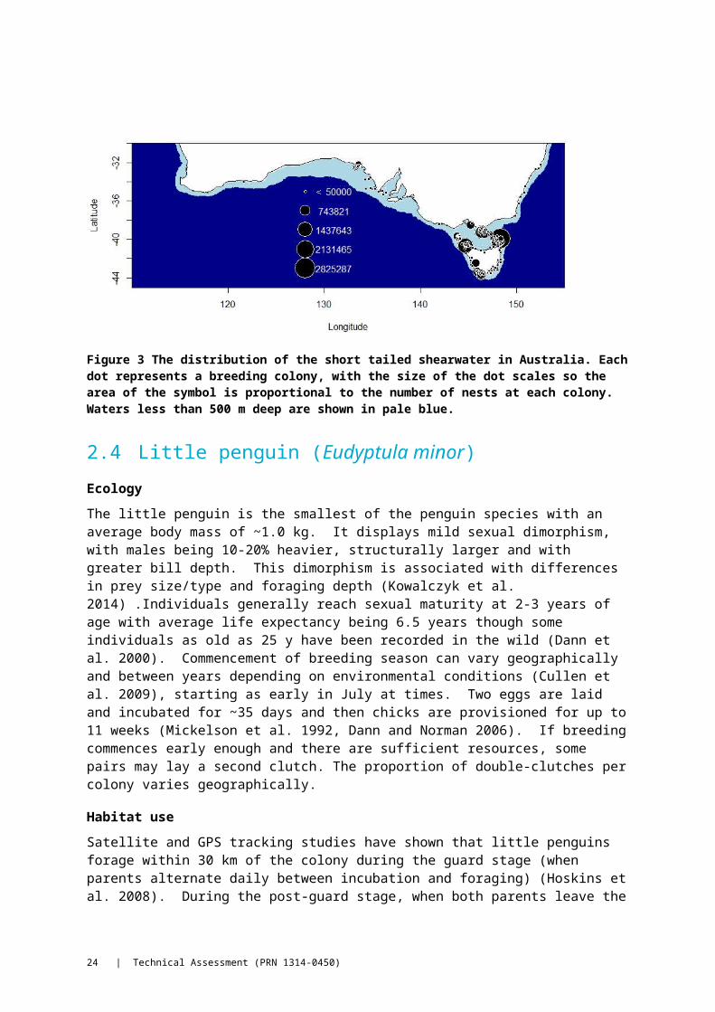
Accurate abundance estimates for the species are lacking, due largely to its burrow nesting breeding strategy and the fact that colonies (>280) are situated on numerous, relatively inaccessible offshore islands (Figure 3). The largest colony, with >2.8 million individuals, is located on Babel Island in eastern Bass Strait. Current population size is estimated to be approximately 23 million individuals though recent studies suggest there has been a substantial decline over the last few decades (Schumann et al. In Press). Nonetheless, it is still Australia’s most abundant seabird and constitutes the second most important marine predator biomass after the Australian fur seal.
Figure 3 The distribution of the short tailed shearwater in Australia. Each dot represents a breeding colony, with the size of the dot scales so the area of the symbol is proportional to the number of nests at each colony. Waters less than 500 m deep are shown in pale blue.
2.4 Little penguin (Eudyptula minor)
Ecology
The little penguin is the smallest of the penguin species with an average body mass of ~1.0 kg. It displays mild sexual dimorphism, with males being 10-20% heavier, structurally larger and with greater bill depth. This dimorphism is associated with differences in prey size/type and foraging depth (Kowalczyk et al. 2014) .Individuals generally reach sexual maturity at 2-3 years of age with average life expectancy being 6.5 years though some individuals as old as 25 y have been recorded in the wild (Dann et al. 2000). Commencement of breeding season can vary geographically and between years depending on environmental conditions (Cullen et al. 2009), starting as early in July at times. Two eggs are laid and incubated for ~35 days and then chicks are provisioned for up to 11 weeks (Mickelson et al. 1992, Dann and Norman 2006). If breeding commences early enough and there are sufficient resources, some pairs may lay a second clutch. The proportion of double-clutches per colony varies geographically.
18 | Technical Assessment (PRN 1314-0450)

DRAFT CONFIDENTIAL TECHNICAL ASSESSMENT (PRN 1314-0450). DO NOT DISTRIBUTE
Habitat use
Satellite and GPS tracking studies have shown that little penguins forage within 30 km of the colony during the guard stage (when parents alternate daily between incubation and foraging) (Hoskins et al. 2008). During the post-guard stage, when both parents leave the nest to feed at the same time, individuals may venture further away from the colony (Kato et al. 2008).
Diet preferences
The diet of little penguins is dominated by small clupeoid schooling fish such as anchovy (Engraulis australis) and sardine (Sardinops sagax), as well as barracouta (Thyrsites atun) and arrow squid (Nototodarus gouldi) (Chiaradia et al. 2010). Average diving depths are 10-20 m but can be deeper (>60 m recorded) (Chiaradia et al. 2007).
Distribution and abundance
The little penguin is one of the most ubiquitous seabirds in southern Australia, being found on most coastal islands throughout its range (Figure 4) in colonies ranging from <50 to >30,000 individuals. They also occur in New Zealand and the Chatham Islands (Marchant and Higgins 1990). In Australia, the total population is currently estimated at ~35000 individuals, with the largest colony located at Gabo Island (Dann and Norman 2006).
Figure 4. The distribution of little penguin breeding colonies in Australia. Each dot represents a breeding colony, with the size of the dot scales so the area of the symbol is proportional to the number of nests at each colony. Waters less than 500 m deep are shown in pale blue.
2.5 Australasian gannet (Morus serrator)
Ecology
The Australasian gannet has nominally been considered monomorphic, with no noticeable difference in plumage between the sexes. However, as with other Sulidae species, recent studies have found females (2.6-2.8 kg) are generally heavier than males (2.4-2.6 kg; Angel and Arnould (in press). Individuals generally reach sexual maturity at 4-7 years of age (though records of younger breeders occur) with a recorded longevity in the wild of 25-38 years (Pyk et al. 2013). Breeding occurs from October-November with one egg being laid. Incubation and chick rearing last 44 and 100-120 days,
Technical Assessment (PRN 1314-0450) | 19

respectively (Pyk et al. 2007). Breeding pairs may attempt re-laying if the egg is lost during incubation.
Habitat use
Recent GPS tracking studies in northern Bass Strait have revealed individuals forage primarily over the continental shelf up to 250 km from the colony during the breeding season though this varies with stage of breeding, geographic location and prey availability (Angel et al. Unpublished data). Using a plunge-diving mode of hunting, gannets can reach depths of 2-4 m but also use underwater wing-flapping to chase prey to even greater depths (Capuska et al. 2011).
Dietary preferences
The main prey of Australasian gannets in Australian waters consist of small schooling species such as barracouta (Thyrsites atun), redbait (Emmelichthys nitidus) and jack mackerel (Trachurus declivis) but they are known to consume squid and numerous other small fish species as well (Bunce and Norman 2000b, Bunce 2001a).
Distribution and abundance
Australasian gannets currently breed at six main locations in south-eastern Australia: Black Pyramid Rocks, Pedra Branca, Eddystone Rock in Tasmania and Lawrence Rocks, Port Phillip Bay and Point Danger in Victoria (Figure 5, Appendix 1.) as well as at numerous sites in New Zealand. In Australia the population was estimated to be at 20,000 pairs in 1999-2000, with the largest colony (12,339 pairs in 1999) located at Black Pyramid Rocks in Tasmania (Bunce et al. 2002). The Australasian gannet population in Australia has been steadily increasing over the last few decades (6% per annum in 2000 (Bunce et al. 2002). Their non-breeding distribution is more widespread with individuals regularly seen in all continental shelf regions around the two countries and the Tasman (Marchant and Higgins 1990).
20 | Technical Assessment (PRN 1314-0450)

DRAFT CONFIDENTIAL TECHNICAL ASSESSMENT (PRN 1314-0450). DO NOT DISTRIBUTE
Figure 5. The distribution of Australasian gannet breeding colonies in Australia. Each dot represents a breeding colony, with the size of the dot scales so the area of the symbol is proportional to the number of nests at each colony. Waters less than 500 m deep are shown in pale blue.
2.6 Australasian sea lion (Neophoca cinerea)
Ecology
The Australian sea lion is the only endemic pinniped in Australia and is the least numerous. The species is unique amongst pinnipeds worldwide due its prolonged and asynchronous breeding schedule (Gales et al. 1994). Females suckle their young for 17-18 months, and the timing of the breeding season (when females are in oesterous and mated by males) varies considerably even among colonies separated by only a few kilometres (Gales and Costa 1997). These attributes make the assessment of basic population parameters such as pup production and trends challenging to quantify (McIntosh et al. 2012).
Habitat use
A number of diving studies have indicated that the Australian sea lions are a predominantly benthically, foraging species (Costa and Gales 2003, Fowler et al. 2006). There is nonetheless considerable inter-individual variation in the habitat use and foraging behaviours among the species, although they can be broadly characterised as either benthic, utilising shallow, coastal waters (<10 m) and offshore, those which forage offshore in waters up to 120 m (Baylis et al. 2008).
Dietary Preferences
There are two conventional diet studies that indicate a broad diet of cephalopods, fish and shark (Gales and Cheal 1992, Baylis et al. 2009). However, each study was conducted at a single site and with a small sample size and therefore provided little information regarding overall diet across the species range. More recent studies using stable isotopes have confirmed the existence of dual foraging strategies; one inshore and shallow water and the other offshore in deeper water (Lowther and Goldsworthy 2011).
Distribution and Abundance
Australian sea lions were listed under the Commonwealth Environment Protection and Biodiversity Conservation Act as Vulnerable in February 2005, and the International Union for the Conservation of Nature has listed then as Endangered. The key threatening process thought to be the demersal gillnet fishery. The total population has been estimated at 11,200 (annual pup production of 2861) (Goldsworthy and Page 2007). Breeding seals are distributed in approximately 72 islands from Houtman Abrolhos in Western Australia to the Pages Islands in eastern South Australia (Figure 6). Most colonies are small, with more than half having annual pup counts of 20 or less. Only eight colonies produce more than 100 pups per breeding cycle, with the largest, Dangerous Reef having approximately 700 pups.
The difficulty in regularly censing colonies due to their remote and dispersed nature combined with the prolonged and asynchronous breeding season means that long term trend data are lacking for the species as a whole. Nonetheless, the several colonies in South Australia for which there are sufficient count data over several years indicate divergent trends among colonies, with the Seal Bay colony, declining, the Dangerous colony increasing and the Pages being stable (Goldsworthy et al. 2009, McIntosh et al. 2013).
Technical Assessment (PRN 1314-0450) | 21
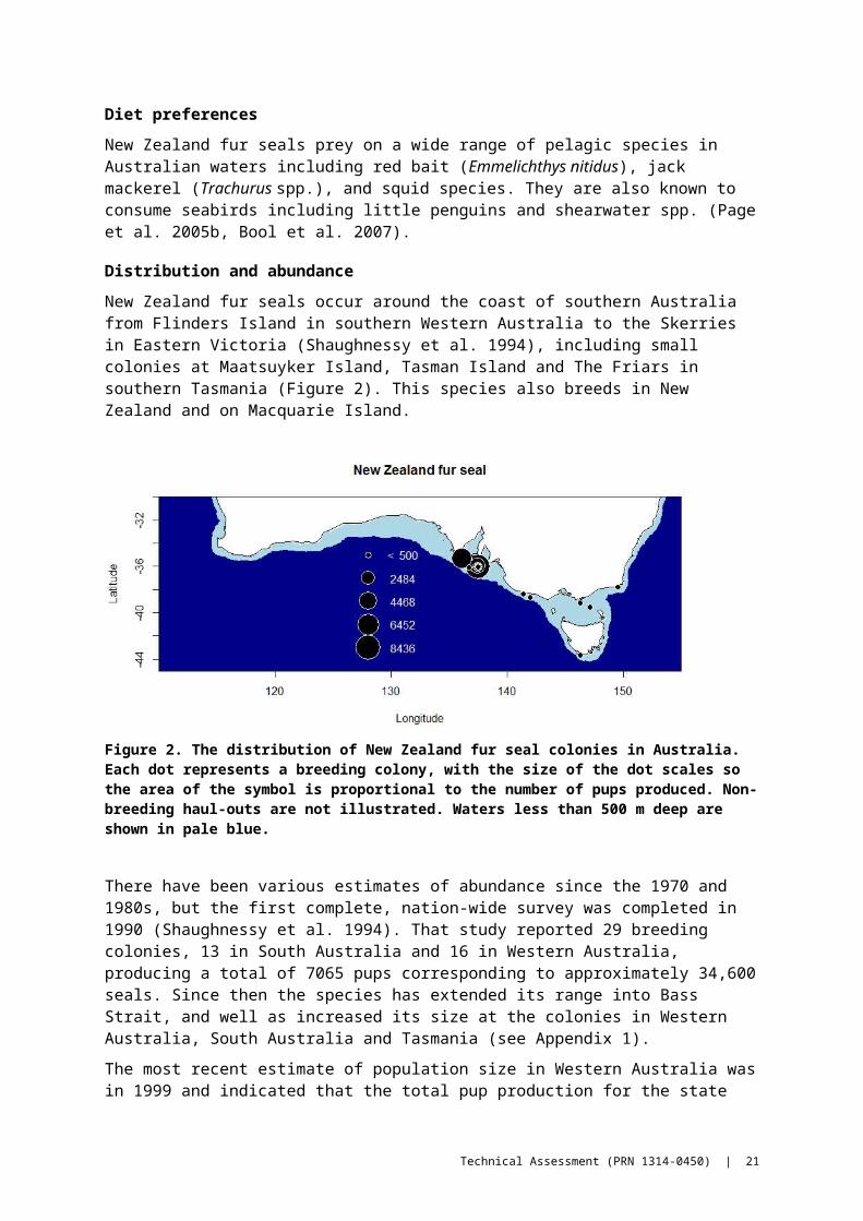
Figure 6 The distribution of Australian sea lion breeding colonies in Australia. Each dot represents a breeding colony, with the size of the dot scales so the area of the symbol is proportional to the number of pups produced at each colony. Waters less than 500 m deep are shown in pale blue.
22 | Technical Assessment (PRN 1314-0450)

DRAFT CONFIDENTIAL TECHNICAL ASSESSMENT (PRN 1314-0450). DO NOT DISTRIBUTE
3 Global examples of spatial management
Small pelagic species in marine ecosystems (e.g. (Cury et al. 2011, Smith et al. 2011)) act as a crucial tropic link in transferring primary production into higher trophic levels (Cury et al. 2000). Therefore it is widely recognized that populations of many marine predators depend on forage species to sustain their populations. Despite this, there are few examples globally where the use of spatial explicit fisheries management has been employed to manage predator populations which consume fisheries target species. Spatial management of fisheries is more common, though the majority of the science underpinning fisheries management is targeted toward single species assessment models. Spatial management issues as a rule, tend to be geared toward management of the target stock and tend to be employed when there is clear evidence of multiple spatial stocks (Begg et al. 1999). Examples of spatial management also exist which aim to minimize ecological impacts such as the effect of bottom trawling on benthic communities (Dunn et al. 2014).
An example from within the SPF is the spatial zoning for conservation of Australian sea lions. These are designed to minimize direct interactions between Australian sea lions and gillnet, hook and trap fisheries in South Australian waters (AFMA 2010). Spatial closures around breeding colonies are based on spatial tracking data and associated at-sea distribution models, and population viability analysis at the colony level (Goldsworthy and Page 2007, Goldsworthy et al. 2010). AFMA has taken a precautionary approach by assuming an overall bycatch of 15 animals per year, allocated differentially across spatial zones (AFMA 2010).
Outside the context of Australian fisheries management, we consider four cases from around the globe where spatial management measures have either been enacted, or are actively being considered as part of fisheries management strategies to reduce potential competition between central place foraging marine species and fisheries which target their prey. These ecosystem-based fisheries management measures can be placed into two broad categories: (i) reactive management in response to predator declines which includes New Zealand and Steller sea lion fishing exclusions, North Sea sandeel fisheries and the South African purse seine fishery; and (ii) precautionary management approaches which includes the Convention for the Conservation of Antarctic Marine Living Resources (CCAMLR) management of the Antarctic krill fishery.
3.1 Reactive management
3.1.1 NEW ZEALAND SEA LIONS, AUCKLAND ISLANDS, NEW ZEALAND
The endemic New Zealand sea lion (Phocarctos hookeri) is listed as Vulnerable by the IUCN in 2008 (Gales 2008). The majority of the population breeds on the Auckland Islands (~86% in 2008) (Chilvers 2008) where the foraging regions of the species overlap with the Southern squid trawl fishery with which considerable by-catch interactions have been documented (Thompson and Abraham 2009). Several measures limiting fishing activities in the region have been adopted. In 1995, a Marine Sanctuary of 12nm surrounding the Auckland Islands was created and in 2003 the area also became a concurrent no take zone (Chilvers 2008). The use of Sea Lion Exclusion Devices (SLEDs) became mandatory in 2003/04. A fishing-related mortality limit (FRML) has also been instituted, and when triggered results in fishery closures (Chilvers 2008). The New Zealand Ministry for Primary Industries and the Department of Conservation are currently engaged in a joint process to deliver a Threat Management Plan (see Figure 7).
Technical Assessment (PRN 1314-0450) | 23

Figure 7 A schematic showing the joint development process for an adaptive Threat Management Plan (TMP) proposed by the NZ Ministry for Primary Industries and the Department of Conservation to address fisheries-induced New Zealand sea lion mortality (see http://www.doc.govt.nz/nzsl-tmp).
3.1.2 STELLER SEA LIONS, NORTH PACIFIC OCEAN, ALEUTIAN ISLANDS
Steller sea lions (SSL) (Eumetopias jubatus) in the North Pacific are the largest otariid pinniped. Amongst its diet are walleye pollock (Gadus chalcogrammus), Pacific cod (Gadus macrocephalus), and Atka mackerel (Pleurogrammus monopterygius) which are also the targets of some of the world’s largest fisheries. The groundfish fishery in this area has a total catch of 2.12 million tonnes and is worth $2.54 M USD (Fissel et al. 2012).
After large declines in abundance, the western distinct population of SSL in Alaskan waters was listed endangered US Endangered Species Act (ESA) in 1997. The eastern distinct population was listed as threatened, although this was recently de-listed (http://www.nmfs.noaa.gov/pr/species/esa/delisted.htm). A range of threats were suggested as proximate causes of the declines, including disturbance at breeding sites, predation by killer whales, climatic shifts, disease and toxins (Williams et al. 2004, Burek et al. 2005, Trites et al. 2007, Atkinson et al. 2008). The likelihood of these threats has been regarded as low compared to a further hypothesis about nutritional stress (Rosen et al. 2000, Rosen and Trites 2002, Trites and Donnelly 2003). Under this hypothesis either natural variability in recruitment or the effects of fisheries, have led to low energy prey species, such as walleye Pollock and Pacific cod, replacing high energy
24 | Technical Assessment (PRN 1314-0450)
DRAFT CONFIDENTIAL TECHNICAL ASSESSMENT (PRN 1314-0450). DO NOT DISTRIBUTE
content prey species such as Pacific herring and Atka mackerel (Sinclair and Zeppelin 2002, Trites et al. 2007). Conn et al. (2014) and Fay and Punt (2006) have noted that this diet change would occur regardless of whether fisheries or natural changes were responsible. However, in the case of natural shifts in prey abundance, there could be few direct fishery management options for assisting the SSL recovery process. Direct manipulation of the ecosystem to experimentally disentangle potential drivers is impossible and so studies have relied on looking for statistical evidence that changes in SSL abundance are related to fisheries activity.
A range of SSL lion protection measures (SSLPM) enforced by the US National Marine Fisheries Service (NMFS) were aimed at ensuring that “the groundfish fisheries off Alaska are not likely to jeopardize the continued existence of the western population of Steller sea lions or adversely modify their critical habitat. The management measures disperse fishing over time and area to protect against potential competition for important Steller sea lion prey species near rookeries and important haul-outs.” (http://alaskafisheries.noaa.gov/protectedresources/stellers/habitat.htm)
Spatial management measures in this area included the use of so-called “critical habitat zones” which consist of a 20 nm (37 km) buffer around all major haul-outs and rookeries and three large offshore foraging zones (Figure 8). In addition 3 nm (5.5 km) no-entry zones have been enacted within which no ground-fishing is allowed. Additionally, within these zones no-transit of vessels is allowed (e.g. see http://alaskafisheries.noaa.gov/rr/tables/tabl12.pdf). Imposing these 3 nm closures has been partly attributed, along with changed fishing practices, to stemming the number of direct interaction mortalities and reducing the rate of decline which was observed after the ESA listing
NOAA has proposed a suite of complex measures for the Bering Sea and Aleutian Island management area which are intended to disperse fishing effort temporally and spatially in this region. The aim is to provide protection from potential competition between the Steller sea lion and fisheries operations (http://alaskafisheries.noaa.gov/prules/79fr37486.pdf).
The proposed management measures in this area are highly complex and operate at a fine-scale relative to the extent of the entire fishery and are enacted on a case-by-case basis by the NMFS.
Technical Assessment (PRN 1314-0450) | 25
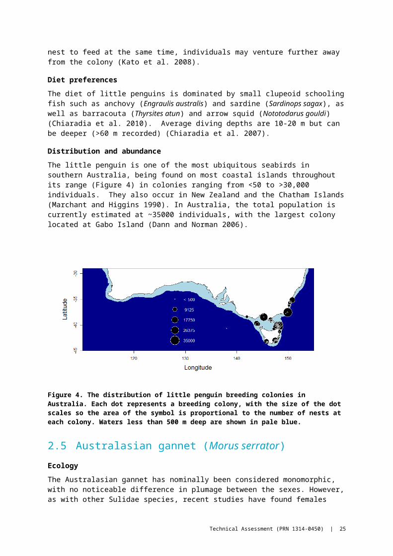
Figure 8 Designated critical habitat zones and exclusion zones around rookeries and haul-outs in the Western Distinct population segment (DPS) for Steller Sea Lions (from NMFS Recovery Plan 2008).
3.1.3 NORTH SEA CLOSED AREAS FOR SANDEELS
The North Sea has historically supported large fisheries of small forage fish species (Engelhard et al. 2014) and also supported a range of predator populations which rely on these (Camphuysen et al. 2006). With the advent of large scale, multi-national fishing operations, there have been significant declines in small pelagic abundance and associated shifts in the ecosystem (Reid et al. 2001, Beaugrand 2004). Many seabirds in the North Sea feed on sandeels (Ammodytes marinus) during their breeding season. Also sandeels are the dominant mid- trophic pelagic fish in the North Sea and no other prey species occurs in similar numbers.
Much of the following material follows a comprehensive overview of the state of the fisheries management and background biology of both seabirds and piscivores provided in the ICES Herring Abundance Working Group (HAWG) reports (Engelhard et al. 2014). The largest single species fishery in the eastern North Sea along the Scottish east coast is the sandeel fishery (in ICES area 4). During the early 1990s, a sandeel fishery developed off the Firth of Forth with landings peaking at over 100,000 t in 1993 before subsequently falling (ICES 2014). This area is important for many breeding seabirds, so the amount landed by the fishery caused concern and the UK called for an EU moratorium on sandeel fishing in areas adjacent to seabird breeding sites. An ICES study group found that there was a suggestion of the fishery causing particularly low seabird breeding in 1993 and recommended a precautionary closure in this region based on the number of seabird breeding colonies it contained and the fact that sandeels in the region comprised a separate stock to other parts of the North Sea. Accordingly the EU directed that the fishery should be closed whilst maintaining commercial monitoring (ICES 2014). A three year closure from 2000-2002 was decided
26 | Technical Assessment (PRN 1314-0450)

DRAFT CONFIDENTIAL TECHNICAL ASSESSMENT (PRN 1314-0450). DO NOT DISTRIBUTE
and based on further reports (Wright et al. 2002), a further three year extension of the closure was decided.
However, since the adoption of the closures, seabird breeding performance in the region has been variable. A range of species delayed their breeding or experienced reproductive failures between 2003-2006 (Frederiksen et al. 2008), and several studies concluded that the main cause for this was a lack of high quality food (Wanless et al. 2005). Since sandeels are known to be the dominant prey for seabirds during the breeding season, there is little doubt that the observed breeding failures were linked to decreased sandeel availability (ICES 2014). Kittiwake breeding has been higher since the fishery closed than in the preceding period, although poor breeding success was observed along the eastern UK coast in 2004 and later evidence has suggested that breeding success may not be a reliable indicator of sandeel availability at some colonies (ICES 2014).
The likely degree of vulnerability of seabirds in the North Sea to fishery effects varies among species. Furness et al. (2012) reviewed North Sea seabird foraging range, diving ability, daily time budgets and ability to switch diet in order to rank each species vulnerability to sandeel depletion. The most vulnerable species were those with poor diving performance, high foraging costs, short foraging range and with little scope to switch their diet. In this case terns, kittiwakes, gulls and skuas were ranked as the most vulnerable, with cormorants, shearwaters and gannet species comprising the least vulnerable. These indices correlated with rankings of breeding success so that species characterized as most vulnerable had lower breeding success measures. These characterizations of vulnerability were supported by the results of several field studies in the region.
Breeding performance of seabirds in the Firth of Forth was generally higher than average since the closure of the sandeel fishery, but there have been difficulties in conducting adequate surveys of sandeel abundance in key areas. Therefore significant uncertainty remains as to the state of the sandeel stocks and the extent to which fisheries or environmental were responsible for breeding failures (ICES 2014).
The latest ICES advice (ICES 2014) suggests that despite uncertainties as to the precise drivers of seabird breeding performance in the area and the possible complications of climatic and environmental shifts, the concern regarding the risks to breeding from sandeel fisheries have not reduced. Without further management controls being adopted there is concern that sandeel aggregations targeted by breeding seabirds could be subject to significant depletion. There is also yet to be a consensus position regarding criteria by which the fishery might be re-opened (ICES 2014).
3.1.4 SOUTH AFRICAN PENGUINS AND SOUTH AFRICAN PURSE SEINE FISHERY
A pelagic purse-seine fishery focused on sardine (Sardinops sagax) and anchovy (Engraulis encrasicolus) has operated in the Benguela and Agulhas current systems off South Africa since the 1940s (Coetzee et al. 2008). The rapid decline in African penguin (Spheniscus demersus) populations, which prey heavily on the fishery target species, prompted the reclassification of the IUCN conservation status of the species as “endangered" in 2010. Importantly, the fishery has also experienced significant spatial shifts in abundance with biomass surveys showing abrupt eastward shifts of sardine spawners. This shift has persisted despite the fact that pre-1998, most adult sardine measured in the November hydroacoustic surveys were found to the west of Cape Agulhas. Between 1997 and 2005, the distribution of sardine catches shifted steadily south and east by a distance of about 400km (Crawford et al. 2006a).
Technical Assessment (PRN 1314-0450) | 27
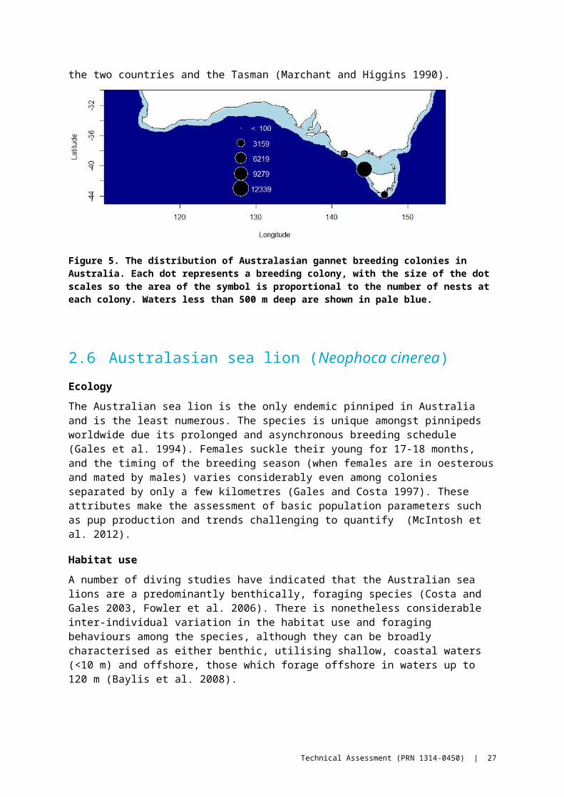
The fishery is managed according to formal management procedure (MP) (Plagányi et al. 2007). The MP relies on survey estimates of recruitment and catch taken prior to recruitment surveys. The current MP is not spatially structured but will be in future.
Recently, there has been increasing pressure on the management system for the South African purse-seine fishery to ensure adequate escapement of anchovy and sardine by setting some threshold on stock abundance below which no catch can be taken to avoid excessive negative impacts on the breeding success of vulnerable predator species such as the African penguin (Crawford et al. 2006b, Cunningham and Butterworth 2006). The development of the next pelagic MP has been subject to diagnostic testing by considering, for example, the risk to penguin populations associated with different levels of pelagic fish catch. Attempts are being made to incorporate functional relationships between predators and prey into the operating models for sardine and anchovy, augmented by population dynamics model(s) for the predator(s) of concern – namely the African penguin.
Interestingly, this is one of the few situations globally to examine the availability of forage species to predators using an experimental approach. An experiment whereby fisheries are alternately allowed entry and excluded in waters surrounding the Robbens and Dassen Island colonies was conducted. Recent analyses (Robinson 2013) have been inconclusive as to whether the breeding success of penguins was actually improved in seasons when a fishery was operating in the area. Additionally, the analysis concluded that survival of adults, as opposed to chicks, was more likely to be a result of prey depletions.
3.2 Precautionary management
3.2.1 ECOSYSTEM-BASED FISHERIES MANAGEMENT OF ANTARCTIC KRILL
The Antarctic krill (Euphausia superba) is a fundamental component of the Antarctic and Southern Ocean food web. Krill is the most important herbivore in the region, and is largely responsible for the trophic transfer of phytoplankton biomass to other Antarctic biota. Baleen whales, seals, fishes, birds and cephalopods are all significant predators of krill. The Antarctic krill fishery is managed by the CCAMLR which is unique in the international management of fisheries because it is a regional management organisation with a conservation remit. It has the attributes of a regional fisheries management organisation (RFMO) but it has a charter to practice ecosystem-based fisheries management with a mandate to explicitly consider the ramifications of management decisions on the broader ecosystem (Constable 2011).
A fishery for Antarctic krill has been operating for over three decades, and has been characterized as one of the world’s largest underexploited fisheries (Nicol et al. 2012). Catches peaked in the 1980s at over 500,000 tonnes annually. Since the early 1990s, the catches have been between 100,000 and 200,000 tonnes with further fishery development being constrained by the expense of fishing in the Southern Ocean and also a limited market for krill products, both of these issues which may be set to change, with increases in catches being perceived as likely (Nicol et al. 2012).
Estimates of abundance of krill to set catch limits have been derived from acoustic surveys (Watkins et al. 2004). Regular time-series have been obtained at smaller scales around the South Shetland Islands on the Antarctic Peninsula (Kinzey et al. 2013) and around South Georgia (Saunders et al. 2007). For example, annual sampling has occurred from 1992 -2011 within an area around the Antarctic Peninsula and recent estimates from acoustic sampling within the western Atlantic and Indian Ocean sectors of the Southern Ocean estimated a total standing stock of 7 million tonnes. The current precautionary catch limit for all Antarctic management areas is 8.6 million tonnes - over 40 times the current catch of approximately 200,000 tonnes (Nicol et al. 2012). In the Scotia Sea, where
28 | Technical Assessment (PRN 1314-0450)

DRAFT CONFIDENTIAL TECHNICAL ASSESSMENT (PRN 1314-0450). DO NOT DISTRIBUTE
the bulk of the fishing occurs, catches are limited by a trigger level of 620,000 tonnes until a procedure for dividing the precautionary total limit for the region of 5.61 million tonnes amongst 15 selected smaller spatial units can be devised (Constable and Nicol 2002, Miller and Agnew 2007, CCAMLR 2012). The trigger level was based on concerns that a regional limit is not sufficient to prevent spatially localized, indirect impacts on krill predators (Constable 2011).
Figure 9 Figure from (Hewitt et al. (2004), Watters et al. (2013))showing the Small-Scale Management Units (SSMUs) in the region of the Antarctic Peninsula and South Georgia.
In practice, the objective specified for the krill fishery consists of two parts, which are to be met simultaneously;
1. A target reference point was established by CCAMLR such that the median status of the spawning stock should not be less than 75% of median spawning biomass prior to fishing in order to account for natural variability. In the absence of sufficient information on predator’s requirements, CCAMLR deemed this target to be appropriate as it was half-way between completely ignoring predator requirements at 50% (determined by the optimum depletion from a Schaeffer surplus production model), and taking full account of predators at 100%, which would entail a fishery take of zero (Constable 2011). In practice, harvesting intensity is adjusted until the median krill spawning biomass is predicted to be 75% of its median pristine size (Thomson et al. 2000).
2. To ensure that the krill were not reduced to a point where the stock could not sustain itself or recover to pre-exploitation abundance, a limit reference point for krill biomass was imposed for which there should only be a low probability of the falling below. This was set to be 20% of the pre-exploitation median biomass (Constable 2011).
At broad scales around the Antarctic, various zones have spatially allocated krill catch limits (Nicol et al. 2012). While these are intended to be explicitly precautionary with regard to ecosystem effects of the fishery, there is yet to be a formal decision rule or management procedure which considers indices of predator population productivity or abundance as part of a feedback into setting Total Allowable Catches (TAC) or in spatial allocation of quota. It is envisaged that this will be formalized in future years and CCAMLR has indicated that this is the system that they are working toward (Constable and Nicol 2002).
One aspect of this is the establishment of 15 Small-Scale Management Units (SSMU, see Figure 9), around the Antarctic Peninsula in FAO area 48 (Constable and Nicol 2002, Hewitt et al. 2004)
Technical Assessment (PRN 1314-0450) | 29

(Constable and Nicol 2002). These are specifically designed to facilitate spatial management options which would operate at a fine scale. These would specifically include separate trigger points to be developed in terms of both catch and metrics of predator performance (CCAMLR 2008). CCAMLR is yet to formalize how these areas are to be managed and is developing a set of candidate decision rules and testing around these (CCAMLR 2011).
The problem of allocating catches between SSMU has been considered by two published studies and extensively by the CCAMLR Scientific Committee (CCAMLR 2011).
Watters et al. (2013) and Plagányi and Butterworth (2007) published what are essentially replicate Management Strategy Evaluation (MSE) exercises which used aggregated “minimum realistic models” (Figure 10). These considered a set of scenarios for spatial movement of predators, functional responses between predator consumption of krill (Figure 11), and krill abundance and also drivers of krill abundance in the region. Additionally, they simulated surveys of krill and predator abundance. Both studies developed a set of reference scenarios which aimed to bound the uncertainty about the true dynamics of the ecosystem and the response of predators to decreases in the krill population. The aim of these was to examine which management responses could meet the necessary simultaneous management objectives for maintain the krill fishery but also for ensuring the persistence of marine predators.
Figure 10 Reproduced from Plagányi and Butterworth (2007) showing the interactions between species and fisheries in their operating model for allocation of catches between 15 Antarctic Peninsula management areas.
30 | Technical Assessment (PRN 1314-0450)

DRAFT CONFIDENTIAL TECHNICAL ASSESSMENT (PRN 1314-0450). DO NOT DISTRIBUTE
Figure 11 Reproduced from Plagányi and Butterworth (2007) showing the model relationship between predator success and krill abundance relative to the average krill carrying capacity. The curves show two examples, one where breeding success in the predators declines near-linearly as krill abundance decreases (squares) and one where breeding success falls steeply only at low krill abundance (line only).
3.2.2 CCAMLR ECOSYSTEM MONITORING PROGRAM (CEMP):
The CCAMLR mandate for ecosystem-based fisheries management necessitates that not only krill catch data be collected, but also that fisheries-independent surveys and monitoring of predators species be carried out. This is done through the CCAMLR Ecosystem Monitoring Program (CEMP). Current monitoring indices are outlined in (CCAMLR 2014 )
The CEMP program has the following aims (i) to detect and record significant changes in critical components of the ecosystem, to serve as a basis for the conservation of Antarctic marine living resources; and (ii) to distinguish between changes due to harvesting of commercial species and changes due to environmental variability, both physical and biological (CCAMLR 2014 )
The program’s largest component is the monitoring of dependent predators species. However, in an attempt to distinguish between potential changes due to fisheries effects and those due to background environmental variability, the program also monitors harvested species, harvesting strategies and environmental parameters.
The program does not monitor all krill dependent species. Instead, it concentrates on a few ‘indicator species’ which are considered more likely to be responsive to changes in the availability of harvested species. These species must be specialist predators on the fishery species, have a broad distribution throughout the Antarctic and/or Southern Ocean and be important ecosystem components. Currently the list includes Antarctic fur seals (Arctocephalus gazella), Adélie (Pygoscelis adeliae), chinstrap (P. Antarctica), gentoo (P. papua) and macaroni penguins (Eudyptes chrysolophus), Antarctic petrel (Thalassoica Antarctica),Cape petrel (Daption capense) and black-browed albatross (Thalassarche melanophrys).
While CEMP uses an extensive set of standard protocols for predator response variables, covering numerous species, sites, and biological parameters (Table 1 , see (Reid et al. 2005) for greater detail, (CCAMLR 2014 )), it can be summarised into several aspects of predator ecology that are monitored on an annual basis: predator diet, foraging behaviour (effort and location), population status (breeding numbers), and reproductive success (fledging/weaning numbers and mass).
Technical Assessment (PRN 1314-0450) | 31

With these parameters are collected on an annual basis, the influence of natural environmental fluctuations on prey availability can, in principal, be separated from anthropogenic factors. An important factor in the CEMP protocols is the annual data collection. This frequency of monitoring enables relatively rapid detection of the influential environmental drivers in variability (Boyd and Murray 2001, CCAMLR 2014 ).
32 | Technical Assessment (PRN 1314-0450)
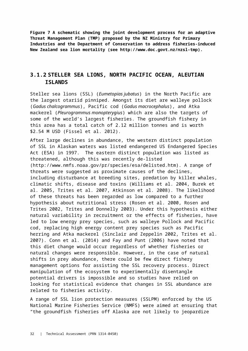
DRAFT CONFIDENTIAL TECHNICAL ASSESSMENT (PRN 1314-0450). DO NOT DISTRIBUTE
Table 1 CEMP Standard methods for monitoring parameters of predator species. KD – Krill dependent, NKD – non-krill dependent.
METHOD PREDATOR TAXA LIFE HISTORY METRIC
A1 Penguins (KD) adult weight on arrival at breeding colony,
A2 duration of the first incubation shift
A3 breeding population size: ground count (A) and aerial counts (B)
A4 age-specific annual survival and recruitment
A5 duration of foraging trips
A6 breeding success
A7 chick weight at fledging
A8 chick diet
A9 breeding chronology
B1 Seabirds (KD) breeding population size
B2 breeding success
B3 age-specific annual survival and recruitment
B4 chick diet
B5 population size, breeding success
B6 adult annual survival and recruitment
C1 Seals (KD) duration of cow foraging/attendance cycles
C2 pup growth
T1 Seabirds (NKD) diet of adult Antarctic shags during the breeding season
Despite the extensive monitoring carried out within CEMP, there is recognition of its limits:
“…at current harvesting levels, it is unlikely that the existing design of CEMP, with the data available to it, will be sufficient to distinguish between ecosystem changes due to harvesting of commercial species and changes due to environmental variability, whether physical or biological…. [it was] recognised that as the fishery increased, it may eventually become possible to detect the impacts of fishing with existing data series, but it would be essential to ensure the fishery operated in areas in which the effects could be detected. It may also be necessary to increase the types of indicators available for feedback management if changes were to be detected more rapidly.”
CCAMLR (2011) p 153.
This problem, whereby two different forcing factors (environmental vs. anthropogenic influences) manifest in indistinguishable ways is a widely recognised issue in the ecosystem approach to fisheries management (Basson 1999).
Technical Assessment (PRN 1314-0450) | 33

34 | Technical Assessment (PRN 1314-0450)

DRAFT CONFIDENTIAL TECHNICAL ASSESSMENT (PRN 1314-0450). DO NOT DISTRIBUTE
4 Methods for at-sea distribution and spatial consumption models
4.1 Preprocessing of telemetry data
In this study, two types of data were considered; Global Positioning System (GPS) data and Argos CLS data. GPS data are highly accurate even for small telemetry devices (generally down to <20m below sea level). Devices with GPS transponders are widely used on seabirds capable of carrying a sufficiently large device. However devices capable of delivering GPS data are a relatively new advance for the tracking of non-seabird species such as pinnipeds. Standard GPS require time to obtain information from satellites in view of the instrument. Fastloc™ GPS is a method which records snapshots of GPS satellite information available during short surfacing interval of an air-breathing marine animal (Costa et al. 2010).
Argos PTT data (Argos 2008) was a precursor technology to GPS, although it is still widely used today. It uses a less accurate method for determining the location of tracked animals based on Doppler shifts of radio transmissions from the telemetry instrument (Argos 2008).
GPS data points are considered to be without significant spatial error and are taken as the true location of an animal. Argos PTT locations are estimated using methods which lead to variable degrees of spatial error, which can often be considerable (Vincent et al. 2002). At sufficiently large spatial scales, save for filtering out gross-outliers, these may be ignored but for fine scale behavioral categorization the errors are likely to be influential and could bias results. Therefore, a state-space correction approach using Kalman filters (Patterson et al. 2010) was applied to the data from New Zealand fur seal and the Australian fur seal data described in (Kirkwood and Arnould 2012).
For diving animals, GPS data are not obtained at regular time intervals. However, regular time-steps are important both for characterizing the amount of time spent within a spatial region and to meet the assumptions of the behavioral switching models (described below). Hence, for the penguin and seal data from GPS, Kalman filters were used as a method for regular interpolation of irregularly spaced GPS time series. Here GPS data were assumed to have minimal error and the movement model underlying the Kalman filter was used to interpolate tracks to provide regular positions. The interpolation time-step varied between species/data set with interpolation based roughly on the frequency of GPS positions in each case.
4.2 Behavioral switching models
Animal movement paths are often decomposed into bouts of behaviour which are thought to relate to underlying behaviour such as foraging or searching. When the movements of an individual animal are characterised by slow speeds with a high degree of turning, this is often termed Area-Restricted Search (ARS) (Fauchald and Tveraa 2003). This movement mode is contrasted by directed movements which tend to be more rapid and with less turning. Here we label these modes as “transit” modes. The reason why these behaviours may be important in this context is that ARS behaviour is more likely to indicate foraging movements and therefore indicate habitats of high-value or preferred conditions for foraging. Hence, we investigated switching between movement behaviours from the available tracking data to examine the distribution of foraging behaviour in terms of distance from colonies. Importantly it allows a comparison of the characteristics of foraging behaviour between species. We examined the proportion of the positions which were categorised in foraging mode at given intervals of distance from the colony.
Technical Assessment (PRN 1314-0450) | 35

For the present study we used only two-dimensional spatial information on predator movements. It is important to note that other behaviours, which might be confounded with ARS behaviours, such as resting behaviours, could not be investigated and would require use of other telemetry data – most likely time-depth recorder data which would indicate when animals were actively diving to pursue prey. For flying seabirds, long periods of sitting on the surface might be indicated by wet-dry sensors (Dean et al. 2012). A recent analysis has examined foraging behaviour using hidden Markov models (HMM) and coupled these to energetic models of foraging (Boyd et al. 2014). We note that more intricate analyses of the tracking data would be an extremely useful addition to the HMM analysis presented here.
To identify ARS behaviour we employed HMMs, a discrete state-space model (Zucchini and MacDonald 2009), which have been applied to animal movement data in several studies (Langrock et al. 2012, McClintock et al. 2012). Following these studies, HMMs were used to decompose movements into two hypothesized latent, or hidden, movement modes; a resident state characterized by relatively slow movements with frequent changes in heading, and a transiting mode of movements which are characterized by more rapid and directed movements. The HMM broadly follow the structure of those considered in (Langrock et al. 2012) and the detailed methods and likelihood calculations for fitting the HMMs are outlined in Patterson et al. (2009). The relevant technical details are briefly provided in Appendix 3.
4.3 Foraging range predictor data collation
For each telemetry location, predictor variables were calculated. These were bathymetry (water depth), the distance to the nearest point on the coast (obtained from http://www.ngdc.noaa.gov/mgg_coastline/), and distance-to-colony following (Goldsworthy and Page 2007). Bathymetry data were obtained from the Geoscience Australia 9-sec resolution bathymetry data set. In addition, we calculated the number of telemetry positions that fell in a 10 km grid square of each telemetry location. For each grid square, an average bathymetric depth was calculated, again from the Geoscience Australia, 9-sec resolution bathymetry product, along with the distance-to-colony and the distance to the nearest coastline point.
4.4 At sea-distribution modelling
At sea distribution models were constructed for major colonies of CPFMP. The timelines of the project precluded a full factorial exploration of diet and colony size. Therefore, we restricted our attention to exploring the model fits for colonies where tracking data were available. Spatial prediction was conducted for Australian fur seal and Australasian gannets in the spatial consumption modelling.
In this study we considered two model types: proximity models following methods outlined in Goldsworthy et al. (2013) and Generalized Additive Models (GAMS)
4.5 Proximity Models
Under this scheme, bathymetry and distance-to-colony are used as predictors of time spent in a region. The probability distribution of these variables was assumed to be modelled using the following density functions:
Pr(Bathymetry = b) ~ Gamma(α, β) (1)
Pr(Distance to colony =d) ~ Normal( μ, σ2) (2)
36 | Technical Assessment (PRN 1314-0450)
DRAFT CONFIDENTIAL TECHNICAL ASSESSMENT (PRN 1314-0450). DO NOT DISTRIBUTE
where
2
22
2)(
exp2
1),,(
ib
bNormal is the Gaussian PDF and
idii eddGamma
1
)(),,(
is the Gamma PDF. The Gamma distribution has properties that the
expected value is
)(xE and
2)(
xVar, so from estimates of α and β, we can compute the
expected value and variance of the fitted PDF. These two PDFs are assumed independent and therefore the
proportion (time spent in region r ) =πr= Pr (Bath=b) × Pr( Dist = d),
i.e. this is simply given as the product of the two models. The proximity models were fitted separately using maximum likelihood estimation, where the likelihood of the data is given by the PDFs (i.e.):
n
i
iibath
bxL
12
22
2)(
exp2
1)|,(
n
i
diidist
ieddL1
1
)()|,(
Numerical minimization of negative log likelihoods was performed using R using the “fitdistr” function in the R library MASS (Venables and Ripley 2002).
4.6 Generalized additive models (GAMs)
GAMs are a widely used class of linear model which allows for non-parameteric smooth modelling in terms of covariates/predictor variables within a generalized linear modelling frame work (Wood 2006). The GAMs considered in this study employed the same predictor variables as the proximity models described in the previous section, and were of the form:
log Nr ~ f ( bathr, distr) + ε (3)
where f(.,.) is a non-parametric bivariate smoothing function and ε is an error term. Thus the GAM models the response variable as a count Nr at a given value of bathymetry or distance. Here we used the most likely estimate of foraging state from the hidden Markov models and used counts of locations categorized as being in foraging mode. The rationale behind this is that we want the GAM to estimate areas most highly utilized in terms of distance to colony and water depth. Since the GAM predicts an expected count, we therefore normalize the
Pr(Time spent in region r) =
rrrr NENE )ˆ(/)ˆ(
(4)
where N̂ r is the model-predicted number of locations expected in region r, to form an estimate of proportion time spent given the predictor variables.
A natural statistical model for counts is the Poisson distribution (McCullagh and Nelder 1989) which assumes that the variance in counts is equal to the mean count. However, given that many of the counts in a grid cell are likely to be zero in the vast majority of grid cells, the data are therefore almost certainly overdispersed, relative to the Poisson. In order to account for this we assumed that counts were distributed according to a Tweedie error distribution which accounts for overdispersion
Technical Assessment (PRN 1314-0450) | 37

(Peel et al. 2013). All generalized additive modelling was conducted using the mgcv library for R (Wood 2006)
For both proximity models and the GAMs, estimating the proportion of a given population of N animals using a given area was done by multiplying the colony size by the time spent in each spatial cell.
4.7 Goodness of model fit
Understanding the performance of models in fitting the existing data is an essential aspect for determining their ability to make reliable predictions in novel locations where data for estimation does not exist. To ascertain how well each these models fit the existing movement data we examined various forms of residuals indicating the degree of goodness-of-fit for each species data.
4.8 Accounting for uncertainty in the spatial models
Using the point-estimates of spatial model parameters could be misleading in determining the degree of precision surrounding spatial predictions of time spent in a given region. Therefore, we conducted a straightforward Monte Carlo procedure to re-sample from fitted models to account for parametric uncertainty. In the case of the proximity models, a standard error on parameter values of the Gamma and Normal distributions (equations 1 and 2) was used to independently draw new parameter values from an assumed Gaussian posterior on the parameters. From these random draws, a set of 1000 spatial predictions was generated from the selected colonies and used to calculate relevant summary statistics, such as mean proportion of time spent and coefficients of variation for spatial prediction regions. A similar approach was performed for the Generalized Additive Models (see Appendix 4).
38 | Technical Assessment (PRN 1314-0450)
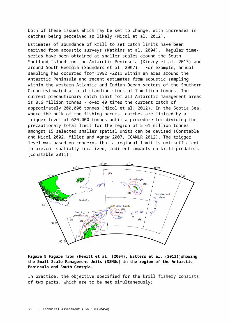
DRAFT CONFIDENTIAL TECHNICAL ASSESSMENT (PRN 1314-0450). DO NOT DISTRIBUTE
5 Spatial model results
5.1 Summary of Bass Strait tracking data used in spatial case studies
The details of tagging deployments of tracking data used in this study are given inTable 2. For some species, a relatively good sample size of individual deployments was available while for others the number was more limited (e.g. New Zealand fur seal). Additionally, some of the tracking data only covered a few years and within these, were limited to short snapshots at particular times of the year (e.g. Little penguin) (Figure 12).
Table 2 Deployment details for tracking data used in case studies. Sample size refers to the number of deployments of tagged animals across all years. The code Platform Transmitter Terminal (PTT) refers to Argos data.
SPECIES COLONY CODE LOCATION SAMPLE SIZE YEARS TRACKING DEVICE
Australian fur seal Kanowna Is GPS AFS 39º10’S, 146º18’E 71 2006-14 Fastloc GPS
Kanowna Is PTT AFS 39º10’S, 146º18’E 14 2001-03 Argos PTT
The Skerries PTT AFS 37º45’S, 149º31’E 11 2001-03 Argos PTT
Lady Julia Percy Is PTT AFS 38º42’S, 142º00’E 12 2001-03 Argos PTT
Seal Rocks PTT AFS 38º30’S, 145º10’E 11 2001-03 Argos PTT
New Zealand fur seal Kanowna Is NZFS 39º10’S, 146º18’E 6 2006-08 Argos PTT
Little penguin Gabo Island GI LP 37°33’S, 149°54 E′ 117 2011-13 GPS
London Bridge LB LP 38°37 S, 142°55 E′ ′ 98 2011-13 GPS
Australasian gannet Pope’s Eye PE GAN 38º16’S, 144º41’E 141 2011-13 GPS
Point Danger DP GAN 38°23 S, 141°38 E′ ′ 69 2011-13 GPS
Short tailed shearwater Griffith Island GI STSW 38°23 S, 142°14 E′ ′ 40 2011-13 GPS
Gabo Island GI STSW 37°33 S, 149°54 E′ ′ 47 2011-13 GPS
Technical Assessment (PRN 1314-0450) | 39

Figure 12 Number of positions per month by species in the Bass Strait tracking data set. The temporal coverage between species varies greatly, indicating that the spatial data used here are snapshots which often only cover small portions of the year and therefore are unlikely to capture seasonal variation. See Table 2for species and deployment location codes.
40 | Technical Assessment (PRN 1314-0450)

DRAFT CONFIDENTIAL TECHNICAL ASSESSMENT (PRN 1314-0450). DO NOT DISTRIBUTE
Figures 13-17 show the spatial extent of the tracking data used in these case studies. Shown in each figure are interpolated positions, which have been filtered with Kalman filters to build a regular time-step data set. For data-rich GPS data sets, this has very little influence on the final positions. For Argos PTT positions, the accuracy of the positions is improved. There are instances of large gaps in the data series (e.g. see the PTT data for AUS; Figure 13). Interpolation artifacts are obvious in these cases and are apparent by long movements in a straight line. Such movements are not realistic representations of true animal movements. In a more refined and detailed analysis, these sections would be removed. In addition, while the accuracy of interpolated positions is a great improvement on the raw Argos data, instances of spatial error remain in the positions. In obvious cases this results in positions predicted to be on land (e.g. Figure 15). These were removed in further analysis.
Another point to note about the interpolation scheme is that it did not filter out positions which were probably haul-outs at locations other than the tagging colony. This only applies to the fur seal data sets. Again, this could be dealt with in a more refined analysis, and for the purposes of this report we expect it to have little impact on the subsequent spatial models. However it is something to be accounted for in future work.
Several general results are apparent. The pinniped data sets (Figure 13 and 14) show movements of a large spatial scale relative to those captured in the seabird data sets (Figures 15-17). Nonetheless there was substantial variation between the two different Australian fur seal data sets. The older set of deployments (i.e. PTT data) from various colonies in Bass Strait captured long movements out of Bass Strait southward along both the west and east coasts of Tasmania as well as movements toward South Australia and NSW coastal regions (Figure 13). Despite being a small dataset, the New Zealand fur seal tracking data indicated similar wide ranging movements and also offshore movements across the continental slope into pelagic waters (Figure 14). Whether this is the norm for New Zealand fur seal in this region is difficult to ascertain due to the small size of the data set.
Figure 13 Interpolated GPS (left) and Argos (right) position data from Australian fur seals (AFS). See Table 2 for deployment locations.
Technical Assessment (PRN 1314-0450) | 41

Figure 14 Interpolated PTT position data from New Zealand fur seals tagged at Kanowna Island.
Figure 15 Interpolated GPS position data from short tailed shearwaters tagged at Gabo Island (GI_STSW) and Griffith Island (GI_STSW).
42 | Technical Assessment (PRN 1314-0450)

DRAFT CONFIDENTIAL TECHNICAL ASSESSMENT (PRN 1314-0450). DO NOT DISTRIBUTE
Figure 16 Interpolated GPS position data from Australasian gannets tagged at Point Danger (PD_gannets) and Pope’s Eye (PE_gannets), Bass Strait.
GILP
-2000
-2000
-2000
-2000
-500
-200
-100
140E 145E 150E 155E
44S
42S
40S
38S
36S
LBLP -2000
-2000
-500 -200
-100
140E 145E 150E 155E
44S
42S
40S
38S
36S
Figure 17 Interpolated GPS position data from little penguins tagged at Gabo Island (GILP) and London Bridge (LBLP). The restricted range of movement is immediately apparent.
The seabird data sets showed more restricted movements and were by in large all on the shelf (Figures 15-17). In some cases, such as little penguins and gannets, this is likely to be a robust characterization of the true scale of movements by these species. For the short tailed shearwater, the restricted scales of the movements are simply due to the breeding phase of the tracked animals, which restricts them to remain close to colonies for chick provisioning. It is also known that short tailed shearwater make long distance foraging trips to Antarctic and Southern ocean waters.
Technical Assessment (PRN 1314-0450) | 43

Additionally, this species makes annual global migrations from the northern hemisphere to breed in southeast Australia. These more complex aspects of the short tailed shearwater foraging and movement strategies are not captured in these data and are therefore not captured in the following spatial distribution and consumption estimates. Hence this report takes an overly simple characterization of foraging and movement in this species. Within the context of spatial management and characterization of the species vulnerability to local depletion, it is likely to overestimate the degree of use and consumption within the SPF. Arguably this presents a more risk adverse picture of their consumption and spatial distribution. Nonetheless, these caveats and limitations are important and should be kept in mind when interpreting modelling results.
For all species, the tracking data indicated that the vast majority of time-at-sea is spent within on-shelf or shelf-break and slope waters. While there were instances of movements beyond the shelf-break, these were in the minority. This is especially likely to hold for animals during intensive periods associated with chick and pup production when areas further afield are inaccessible without causing reductions in breeding success or biparental investment in growth of young.
The case study data sets also do not capture the characteristics of many colonies. For example, the little penguin and short tailed shearwater tracking datasets are both relatively close to the shelf edge, compared to other colonies. For other colonies which are further from shelf edge and oceanic habitat, foraging distributions and also available and important prey types are likely to differ markedly.
Whether or not these aspects are important for spatial management is unclear, but this point indicates that spatial data sets with sufficient contrast in habitat type and accessibility were not available for this project and are generally not collected. As a result, it is apparent that spatial models and the conclusions drawn from their results may not be reliably transportable to areas where tracking data are not available.
Figure 18 shows the within species variability in distance of locations from the tagging location/colony. The summary statistics of these are given in Table 3. Generally there was very large within species variation. Mean distances from a colony are probably unreliable as a summary statistic for characterizing foraging range. However, in the case of little penguins, all locations were within 50 km of the colony and suggest that between individual variability in movement is probably unimportant for spatial questions at scales relevant to spatial management. This is likely not the case for other species, pinnipeds in particular. Figure 19 shows the range of water depths/bathymetry utilized by CPFMP in the case study data. Despite, overall trends and the tendency for animals to vastly favor water on the shelf and less than 200m there was a high degree of variability between individuals.
44 | Technical Assessment (PRN 1314-0450)
DRAFT CONFIDENTIAL TECHNICAL ASSESSMENT (PRN 1314-0450). DO NOT DISTRIBUTE
0 10 20 30 40
020
4060
80Cdist: AUFS
ID
Dis
tanc
e to
col
ony
(km
)
2 4 6 8 10 14
510
1520
25
Cdist: GI_STSW
ID
Dis
tanc
e to
col
ony
(km
)
0 20 40 60 80 100
010
2030
40
Cdist: GILP
ID
Dis
tanc
e to
col
ony
(km
)
1 2 3 4 5 6
010
3050
Cdist: GR_STSW
ID
Dis
tanc
e to
col
ony
(km
)
0 20 40 60 80
515
2535
Cdist: LBLP
ID
Dis
tanc
e to
col
ony
(km
)
1 2 3 4 5
010
020
030
0
Cdist: NZFS
ID
Dis
tanc
e to
col
ony
(km
)
0 10 20 30 40
050
150
Cdist: PD_gannet
ID
Dis
tanc
e to
col
ony
(km
)
0 20 40 60 80
020
6010
0
Cdist: PE_gannet
ID
Dis
tanc
e to
col
ony
(km
)
0 10 20 30 40 50
010
030
0Cdist: PTT_AUFS
ID
Dis
tanc
e to
col
ony
(km
)
Figure 18 Individual average distance-to-colony by tag-deployment/individual for each species. Also shown (red dotted line) is the average distance from the colony. See Table 2 for species and deployment location codes.
Technical Assessment (PRN 1314-0450) | 45
0 10 20 30 40
-200
-100
0Bathy : AUFS
ID
bath
ymet
ry(m
)
2 4 6 8 10 14
-200
-100
0
Bathy : GI_STSW
ID
bath
ymet
ry(m
)
0 20 40 60 80 100
-200
-100
0
Bathy : GILP
ID
bath
ymet
ry(m
)
1 2 3 4 5 6
-200
-100
0
Bathy : GR_STSW
ID
bath
ymet
ry(m
)
0 20 40 60 80
-200
-100
0Bathy : LBLP
ID
bath
ymet
ry(m
)
1 2 3 4 5
-200
-100
0
Bathy : NZFS
ID
bath
ymet
ry(m
)
0 10 20 30 40
-200
-100
0
Bathy : PD_gannet
ID
bath
ymet
ry(m
)
0 20 40 60 80
-200
-100
0
Bathy : PE_gannet
ID
bath
ymet
ry(m
)
0 10 20 30 40 50
-200
-100
0Bathy : PTT_AUFS
ID
bath
ymet
ry(m
)
Figure 19 Bathymetry range by individual tag deployment within each species /data set. Average bathymetry value is given by the red-line. See Table 2 for species and deployment location codes.
Table 3 Summary statistics by species and data type for case study tracking data. See Table 2 for species and deployment location codes.
SPECIES/DATASET AVERAGE COLONY DISTANCE (KM)
(SD) AVERAGE BATHYMETRY (-M)
(SD)
AFS (Kanowna Is., GPS) 18.226 44.974 -34.489 19.626
AFS (Various colonies, PTT) 120.564 142.467 -48.252 70.499
STSW (GR, GPS) 6.855 20.092 -12.008 95.418
STSW (Gabo Island, GPS) 7.671 11.939 -27.613 26.853
LP (Gabo Island, GPS) 16.611 15.679 -131.043 283.535
LP (London Bridge, GPS) 10.142 9.329 -49.069 21.662
NZFS (PTT) 22.960 95.868 -34.017 192.828
GAN (Point Danger, GPS) 30.164 71.481 -58.120 392.125
GAN (Pope's Eye, GPS) 19.462 37.712 -9.650 22.141
46 | Technical Assessment (PRN 1314-0450)

DRAFT CONFIDENTIAL TECHNICAL ASSESSMENT (PRN 1314-0450). DO NOT DISTRIBUTE
5.2 Habitat summaries
For this analysis, distance-to-colony and bathymetry were used as predictors of spatial distribution (see below). We now present summaries of these covariates by species. It is again important to note, that bathymetry per-se is likely to be of limited biological relevance to many of these species, beyond the fact that it is useful in restricting model predictions to plausible zones off-shore.
A useful summary of the colony distance and bathymetry ranges selected or available to the predator species is to create a 2-dimensional histogram of the number of locations falling jointly within particular range of bathymetry and distance-from-colony. Figures 20-24 shows these for each predator species. One reason why these plots are useful is that by visually depicting the joint-distribution of these two variables, they give an indication of whether the data are likely to meet the assumptions of the proximity models and GAMs, results from which are described below, which make different assumptions regarding the statistical independence of distance-to-colony and bathymetry. For proximity models to fit the data well, the joint distributions of these data need to indicate little correlation and most of the data falling within an elliptical region centered on the expected values of the probability density functions (PDF) pertaining to distance-to-colony and bathymetry. GAMs are potentially more flexible but also liable to be influenced by outliers and this very flexibility may lead to unsupported inferences of the proportion of time spent in a given habitat regime.
The distribution of colony distance and bathymetry was generally complex and interdependent for all species. The Australian fur seal GPS data (Figure 20, left) showed a region around 80m deep which was heavily utilized by these animals. This was important over a range of colony distances. Such a joint distribution reflects that in this data set the animals largely remained within central Bass Strait and adopt a predominantly benthic foraging strategy (Arnould and Kirkwood 2008). For the Australian fur seal PTT data (Figure 20, right), on the other hand, the spatial distribution was much more complex with animals foraging at a range of depths and down to deeper depths, which is indicative of the wide range of locations utilized by this species.
The same plot for New Zealand fur seal (Figure 21) largely reflected the small size of the tagging data set available for this work, but reflected that the animals spent long bouts of time close to shore over shallow water with excursions into deeper off-shelf waters
Technical Assessment (PRN 1314-0450) | 47

0 100 200 300 400 500
-100
-80
-60
-40
-20
0PTT AFS
distance to colony (km)
Bat
hym
etry
(m)
0
20
40
60
80
100
120
140
0 20 40 60 80 100 120 140
-100
-80
-60
-40
-20
0
AFS
distance to colony (km)
Bat
hym
etry
(m)
0
5
10
15
20
25
Figure 20 Joint histograms of number of locations at a given colony distance and bathymetry range for Australian fur seal. Left hand side is the GPS data from Kanonwa Island Right hand side is the early PTT data from various Bass Strait colonies.
0 50 100 150 200
-100
-80
-60
-40
-20
0
NZFS
distance to colony (km)
Bat
hym
etry
(m)
0
2
4
6
8
Figure 21 Joint histograms of number of locations at a given colony distance and bathymetry range for New Zealand fur seal. Note the low sample sizes associated with sparse position data.
For short tailed shearwater (Figure 22), the joint distributions of distance-to-colony and bathymetry were generally complex. For birds tagged at Gabo Island, the joint distribution was relatively clustered with most of the distances less than 60km from the colony, and in waters of 0-100m depth being chiefly utilized. The data from Griffith Island showed more outliers resulting from birds making longer offshore trips at this colony.
48 | Technical Assessment (PRN 1314-0450)

DRAFT CONFIDENTIAL TECHNICAL ASSESSMENT (PRN 1314-0450). DO NOT DISTRIBUTE
0 20 40 60 80 100 120 140
-200
-150
-100
-50
0GR STSW
distance to colony (km)
Bat
hym
etry
(m)
0
2
4
6
8
10
0 20 40 60 80 100
-200
-150
-100
-50
0
GI STSW
distance to colony (km)
Bat
hym
etry
(m)
0
2
4
6
8
Figure 22 Joint histograms of number of locations at a given colony distance and bathymetry range for short tailed shearwater. Left hand side is the data from Gabo Island. Right hand side is from Griffith Island.
Little penguin joint-histograms (Figure 23) showed that animals spent time mostly in shallow waters close to the colony; although the data from Gabo Island showed a greater degree of variability. Nonetheless, based purely on these visual summaries, of all the data considered here the little penguin data appear the most in accord with the assumptions of the proximity models.
Data from gannets (Figure 24) was variable both between the two colonies where tagging occurred and within these colonies. The Pope’s Eye colony was generally more restricted to foraging closer to home and within central Bass Strait, which was reflected in the range of bathymetric values. Point Danger birds foraged further from the colony and over a more variable range of bathymetric habitats.
0 20 40 60 80 100
-200
-150
-100
-50
0
GI LP
distance to colony (km)
Bat
hym
etry
(m)
0
5
10
15
20
25
0 20 40 60 80 100
-200
-150
-100
-50
0
LBLP
distance to colony (km)
Bat
hym
etry
(m)
0
10
20
30
40
50
Figure 23 Joint histograms of number of locations at a given colony distance and bathymetry range for little penguins. Left hand side is the data from London Bridge. Right hand side is from Gabo Island.
Technical Assessment (PRN 1314-0450) | 49

0 50 100 150 200
-100
-80
-60
-40
-20
0PE GA
distance to colony (km)
Bat
hym
etry
(m)
0
50
100
150
200
Figure 24 Joint histograms of number of locations at a given colony distance and bathymetry range for Australasian gannets. Left hand side is the data from Point Danger. Right hand side is from Pope’s Eye.
50 | Technical Assessment (PRN 1314-0450)

DRAFT CONFIDENTIAL TECHNICAL ASSESSMENT (PRN 1314-0450). DO NOT DISTRIBUTE
5.3 Behavioral switching model results
Because plots of large amounts of tracking data can be difficult to interpret, kernel density estimation (KDE, Venables and Ripley (2002)) was used to visually summarize the spatial distribution of locations which were highly likely to be classified as foraging bouts (a threshold of P(ARS) = 0.7 was used to select these). The KDE methods are not particularly useful beyond providing a simple visual summary of areas with intensive ARS activity.
In general, the HMMs were able to pick out bouts of ARS-like behavior quite well, although this varied between species and data sets. The Australian fur seal GPS data (Figure 25) showed a large degree of intensive spatial usage within central Bass Strait, although a few tracks did traverse eastwards to forage over the shelf break. The KDE (Figure 25B) also highlights that this analysis did not account for likely haul-outs at colonies other than the location of tagging, with clear visits to coastal locations in northwest Tasmania. These could be dealt with and are unlikely to greatly influence the results.
The Australian fur seal PTT data, being much more dispersed, showed a tendency for animals to forage over the shelf break, especially on the western side of Bass Strait (Figure 26). The KDE summary (Figure 26B) therefore showed a much more diffuse range of foraging locations with no clear central focus, in contrast to the Australian fur seal data shown in Figure 25.
The New Zealand fur seal data, being less numerous Argos CLS data, was generally uninformative regarding locations of ARS type movements. Areas which did contain intensive ARS behavior (Figure 27) were probably haul-outs and therefore can be ruled out. This indicates that any distribution modelling based on such data is likely to be uninformative for the aims of this study. We do fit such models (see below) but it is clear that much more data are required for adequate characterization of at-sea distribution or in examining where ARS behavior occurs.
For short tailed shearwaters at Gabo Island, the results of the HMMs were mixed. Seabirds with high rates of travel can be difficult subjects for HMM because sampling is often too infrequent to detect rapid changes in behavior. In this case (Figure 28A) several artifacts of interpolation from Kalman filtering results also limit the usefulness of the modelling, as positions were predicted ashore. Nonetheless, all bouts of ARS were placed offshore but in close proximity to the colony. The KDE (Figure 28B) reflected this distribution close to the colony.
Griffith Island shearwaters similarly displayed a tendency to foraging largely inshore (Figure 29A). Visual inspection seems to indicate that these data sets provided more plausible movement tracks than those from Gabo Island. Notable were excursions to deeper off-shelf waters. The KDE (Figure 29B) shows the inshore distribution
Australasian gannets from Pope’s Eye forage over a range of distances from the colony (Figure 30A). The KDE suggested that focus of ARS activity was close to the colony. However in this case the KDE seems a poor guide of the distribution of intensive foraging. Animals undertook long foraging trips almost to northern Tasmania. Generally the shelf break was not targeted.
Similarly, gannets from Point Danger were restricted to on-shelf and slope waters (Figure 31A). There were occasional forays into deeper water but these were rare. Animals did travel reasonably long distances but stayed over shelf waters at nearly all times.
Unsurprisingly the foraging range of little penguins was the smallest of all species considered here (Figure 32 and Figure 33). The Gabo Island tracks (Figure 32) show occasional sorties away from the colonies but the vast majority was very close to the colony.
Technical Assessment (PRN 1314-0450) | 51
(A)
(B)
Figure 25 (A) Behaviour switching model results for Australian fur seals (GPS data – see Table 2 for deployment locations). Large red dots indicate high probability of ARS mode and small blue dots indicate low ARS probability (high probability of transit mode) (B) Spatially smoothed ARS locations (includes only locations where Prob(ARS) > 0.7).
52 | Technical Assessment (PRN 1314-0450)

DRAFT CONFIDENTIAL TECHNICAL ASSESSMENT (PRN 1314-0450). DO NOT DISTRIBUTE
(A)
(B)
Figure 26 (A) Behaviour switching model results for Australian fur seals (PTT data – see Table 2 for deployment locations). Large red dots indicate high probability of ARS mode and small blue dots indicate low ARS probability (high probability of transit mode) (B) Spatially smoothed ARS locations (includes only locations where Prob(ARS) > 0.7).
Technical Assessment (PRN 1314-0450) | 53
Figure 27 Behaviour switching model results for New Zealand fur seals (Argos CLS data – see Table 2 for deployment locations). Large red dots indicate high probability of ARS mode and small blue dots indicate low ARS probability (high probability of transit mode). Kernel smoothing was not performed because of few data points.
54 | Technical Assessment (PRN 1314-0450)

DRAFT CONFIDENTIAL TECHNICAL ASSESSMENT (PRN 1314-0450). DO NOT DISTRIBUTE
(A)
(B)
Figure 28 (A) Behaviour switching model results for short tailed shearwaters from Gabo Island (GPS data – see Table 2 for deployment locations). Large red dots indicate high probability of ARS mode and small blue dots indicate low ARS probability (high probability of transit mode). (B) Spatially smoothed ARS locations (includes only locations where Prob(ARS) > 0.7).
Technical Assessment (PRN 1314-0450) | 55
(A)
(B)
Figure 29 (A) Behaviour switching model results for short tailed shearwaters from Griffith Island (GPS data – see Table 2 for deployment locations). Large red dots indicate high probability of ARS mode and small blue dots indicate low ARS probability (high probability of transit mode). (B) Spatially smoothed ARS locations (includes only locations where Prob(ARS) > 0.7).
56 | Technical Assessment (PRN 1314-0450)

DRAFT CONFIDENTIAL TECHNICAL ASSESSMENT (PRN 1314-0450). DO NOT DISTRIBUTE
(A)
(B)
Figure 30 (A) Behaviour switching model results for gannets from Pope’s Eye (GPS data – see Table 2 for deployment locations). Large red dots indicate high probability of ARS mode and small blue dots indicate low ARS probability (high probability of transit mode). (B) Spatially smoothed ARS locations (includes only locations where Prob(ARS) > 0.7).
Technical Assessment (PRN 1314-0450) | 57

(A)
(B)
Figure 31 (A) Behaviour switching model results for gannets from Point Danger (GPS data – see Table 2 for deployment locations). Large red dots indicate high probability of ARS mode and small blue dots indicate low ARS probability (high probability of transit mode). (B) Spatially smoothed ARS locations (includes only locations where Prob(ARS) > 0.7).
58 | Technical Assessment (PRN 1314-0450)

DRAFT CONFIDENTIAL TECHNICAL ASSESSMENT (PRN 1314-0450). DO NOT DISTRIBUTE
(A)
(B)
Figure 32 (A) Behaviour switching model results for little penguins from Gabo Island (GPS data – see Table 2 for deployment locations). Large red dots indicate high probability of ARS mode and small blue dots indicate low ARS probability (high probability of transit mode). (B) Spatially smoothed ARS locations (includes only locations where Prob(ARS) > 0.7)
Technical Assessment (PRN 1314-0450) | 59

(A)
(B)
Figure 33 (A) Behaviour switching model results for little penguins from London Bridge (GPS data – see Table2 for deployment locations). Large red dots indicate high probability of ARS mode and small blue dots indicate low ARS probability (high probability of transit mode). (B) Spatially smoothed ARS locations (includes only locations where Prob(ARS) > 0.7)
60 | Technical Assessment (PRN 1314-0450)

DRAFT CONFIDENTIAL TECHNICAL ASSESSMENT (PRN 1314-0450). DO NOT DISTRIBUTE
5.4 Proportion of foraging effort at distances from the colony
Examining how the proportion of time spent foraging increases to 100% with distance from the colony illustrates how the CPFMP allocated their time between ARS and transit modes (Figure 34). All seabird species spent at least 50% of their foraging time at ranges less than 50km. Similarly, the seabirds allocated at least 80% of their foraging effort within 100km of colonies (Table 4, Figure 34).
Pinnipeds foraging effort was allocated at larger distances from colonies, with some variability between Australian fur seal datasets. For the GPS Australian fur seal data from Kanowna Island, 50% of foraging occurred within 83 km of the colony. For the PTT data the same figure was nearly twice as high (Table 4). The New Zealand fur seal showed the highest foraging ranges at the 80% level, but the distance containing 50% of foraging effort was less than the Australian fur seal PTT data (Figure 35). It is worth recalling that the New Zealand fur seal tracking data used here is limited and these results should be treated with caution
Figure 34 Cumulative distributions of percentage time spent in ARS mode as a function of distance-to-colony. This plot can be used to infer the amount of time spent foraging within a given radius of distance to colony (see Table 4, Figure 35below). See Table 2 for species and deployment location codes.
Technical Assessment (PRN 1314-0450) | 61

Table 4 Distance to colony radius (km) containing 20, 50, or 80 % of ARS (“foraging” mode) locations by CPFMP species.
SPECIES 20% 50% 80%
Gabo Island STSW 1.34 1.44 12.46
London Bridge LP 4.02 9.19 15.09
Gabo Island LP 6.19 13.24 23.66
Pope’s Eye gannet 3.57 15.97 56.70
Griffith Island STSW 8.13 41.13 74.60
Point Danger gannet 6.87 35.53 100.09
Kanowna Island AFS (GPS) 38.39 82.35 158.54
PTT AFS 122.49 233.04 298.44
NZFS 151.04 151.04 331.34
GI_
STS
W
LBLP
GIL
P
PE
_gan
net
GR
_STS
W
PD
_gan
net
AU
FS
PTT
_AU
FS
NZF
S
Dis
tanc
e to
col
ony
(km
)
0
100
200
300
40020%50%80%
62 | Technical Assessment (PRN 1314-0450)

DRAFT CONFIDENTIAL TECHNICAL ASSESSMENT (PRN 1314-0450). DO NOT DISTRIBUTE
Figure 35 Distance to colony radius (km) containing 20%, 50%, or 80% of ARS (“foraging” mode) locations by CPFMP species.
5.5 At sea distribution model results
Both the proximity models (Figure 36-41))and the GAMs (Figure 42 and Figure 43 )seemed to capture the general distribution of the tagging data for each species. The proximity models seem to over- emphasize locations close to colonies relative to the data. This may be due to the use of the Gamma PDF to model time spent at a given distance from the colony. GAMS, being generally more flexible, showed some indications of edge effects when predicting across a spatial grid.
The Gamma PDFs fit the distribution of distance-to-colony best in the case of the little penguin data (Figure 376 and Figure 387). Other species (e.g. Pope’s Eye gannets - Figure 38) displayed indications of two distributions in the time-spent at given distances from the colony. For these models, the fitted gamma PDFs may be too limited a model to capture time-spent at relatively distant locations. Similarly, some fits to bathymetry data were generally poor with large outliers. Data from Gabo Island short tailed shearwater gave probably the best fit, but even here, the uni-modal Gaussian distribution seemed like an inadequate model for these data. We conclude that bathymetry is useful as a predictor variable, as it restricts the foragers to on-shelf waters, but its utility as a predictor of preferred foraging habitat seems limited. A clear example of the issues involved can be seen in the fit of the Gaussian PDF to the bathymetry data from Pope’s Eye gannets (Figure 38). Here, the data has a “u-shape” with peaks in very shallow water and again at around 70 m depth. The normal PDF has an expected value of -43m, which is in the middle of the two peaks where there is little data.
The parameters of the proximity models were apparently well estimated with low standard errors on the parameters (Table 5). The models also seemed to reliably model the general features of the distribution of distance-from-colony, with the expected colony distances being in line with the dispersal capacity of the species; Australian fur seal, New Zealand fur seal had the highest mean distances from the colony (Table 5), with the little penguin estimates being the lowest (both colonies had an expected distance to colony <20km). The issues with the fits to the bathymetric data notwithstanding, the mean depths estimated were roughly in accordance with the results for foraging distance, with predators which disperse further generally having a deeper associated expected depth (Table 5). The expected depths naturally also reflected the proximity of the colony to the shelf edge. For example Gabo Island little penguin had an estimated mean foraging depth of -126m whereas the value for London bridge little penguin was about half that. This sort of phenomena points to local colony characteristics being important in describing the types of conditions used for foraging. This is not surprising, as it has been widely recognized that selected foraging habitat for animals is a tradeoff between preference and accessibility in several tracking studies (Sharples et al. 2012) and in spatial modelling studies (Matthiopoulos et al. 2004).
This point has implications for using at-sea models in management applications. If, as in the case of this study, the tracking data are not ‘synoptic’ (i.e. derived from a wide range of sites within the management zone), it is possible that any spatial models developed from such data are not transportable or representative of the distribution and behavior in other areas. From the data at hand and the constraints on the scope of this report, we cannot determine how important this is likely to be, even for the Bass Strait and surrounding regions. It is clear that there is a large degree of variation in behavior. But whether this is sufficiently acute to be problematic for spatial management is likely to depend on the scale and particular locations of any management measures (e.g. the size of say a spatial closure region).
Technical Assessment (PRN 1314-0450) | 63

AUFS
cdist
Den
sity
0 50 100 150 200
0.00
00.
004
0.00
8AUFS
bath
Den
sity
-120 -100 -80 -60 -40 -20 0
0.00
0.02
0.04
GI_STSW
cdist
Den
sity
0 20 40 60 80
0.00
00.
010
0.02
00.
030
GI_STSW
bath
Den
sity
-150 -100 -50 0
0.00
00.
005
0.01
00.
015
GILP
cdist
Den
sity
0 20 40 60 80
0.00
0.01
0.02
0.03
0.04
GILP
bath
Den
sity
-3000 -2500 -2000 -1500 -1000 -500 0
0.00
00.
002
0.00
4
Figure 36 Proximity model fits by species. The left hand columns are the fits of the Gamma PDF to the distance from colony; right hand column shows the fits of a Gaussian PDF to the bathymetry data. See Table2 for species and deployment location codes.
64 | Technical Assessment (PRN 1314-0450)

DRAFT CONFIDENTIAL TECHNICAL ASSESSMENT (PRN 1314-0450). DO NOT DISTRIBUTE
GR_STSW
cdist
Den
sity
0 20 40 60 80 100 120
0.00
00.
005
0.01
00.
015
GR_STSW
bath
Den
sity
-1500 -1000 -500 0
0.00
00.
002
0.00
4
LBLP
cdist
Den
sity
0 10 20 30 40 50 60 70
0.00
0.02
0.04
0.06
LBLP
bath
Den
sity
-150 -100 -50 0
0.00
0.01
0.02
0.03
0.04
NZFS
cdist
Den
sity
0 100 200 300 400 500 600 700
0.00
00.
004
0.00
8
NZFS
bath
Den
sity
-5000 -4000 -3000 -2000 -1000 0
0.00
000.
0010
Figure 37 Continued results from Figure 36
Technical Assessment (PRN 1314-0450) | 65

PD_gannet
cdist
Den
sity
0 100 200 300
0.00
00.
004
0.00
8PD_gannet
bath
Den
sity
-5000 -4000 -3000 -2000 -1000 0
0.00
000.
0010
PE_gannet
cdist
Den
sity
0 50 100 150 200 250 300 350
0.00
00.
005
0.01
00.
015
PE_gannet
bath
Den
sity
-80 -60 -40 -20 0
0.00
00.
010
0.02
00.
030
PTT_AUFS
cdist
Den
sity
0 200 400 600 800
0.00
000.
0010
0.00
200.
0030
PTT_AUFS
bath
Den
sity
-5000 -4000 -3000 -2000 -1000 0
0.00
000.
0010
Figure 38 Continued results from Figure 36 and 37.
66 | Technical Assessment (PRN 1314-0450)
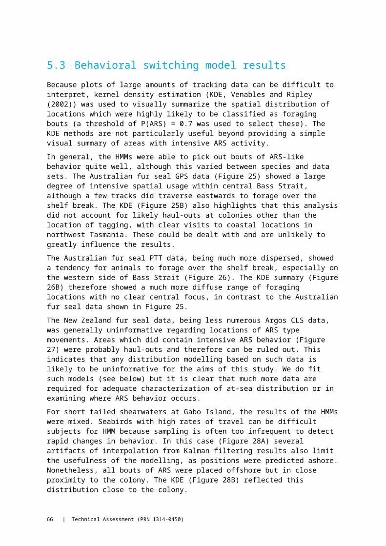
DRAFT CONFIDENTIAL TECHNICAL ASSESSMENT (PRN 1314-0450). DO NOT DISTRIBUTE
Figure
39 Continued results from Figure 38 for AFS PTT data by colony.
Technical Assessment (PRN 1314-0450) | 67

It is highly likely that low SE on proximity model parameters is an artifact of the models assuming that each data point of bathymetry or distance-to-colony is statistically independent from the other data. Movement data are notoriously auto-correlated and non-linear. Over shorter time scales, even wide ranging animals are most likely close to where they were at a previous instance in time.
The net effect of incorrect assumption of independence is that uncertainty estimates around the parameters of the proximity models are almost certainly under-estimates. This means that sampling from these models to assess the variability in proportion time spent will be biased low. In effect, the models assume that the data contain greater information content than they really do. This means that estimates of uncertainty, when propagated into consumption models, will probably lead to underestimates of CVs.
Note that this problem applies equally to the GAMs used here. It may be ameliorated to a small degree by using the HMM categorizations of ARS, which would have the effect of removing parts of the movement data and increasing the chance of breaking serial dependence. On the other hand, for long bouts of ARS behavior, the problem will be similar to the issues with proximity models. Essentially any reduction in autocorrelation of the movement data, which might be afforded by using only ARS categorized locations, is only by accident.
Further exploration of model uncertainty should at least examine the effect of artificially inflating the SEs on model parameters to see how this propagates into spatial consumption estimation. A better strategy would be to employ models which can account for autocorrelation in the movement data, ideally by modelling the structure of CPFMP trips. This would be a detailed modelling exercise, and really only worth considering for predators which make long distance movements. The penguin tracking data were adequately described for the purposes required here – to determine the extent of foraging range- and distance from colony measures alone (such as the maximum distance from a colony or 80th percentile of distances from colonies) would probably suffice in capturing the relevant aspects of their distribution. For other species more complex models may be required.
For the context at hand, the nuances surrounding statistical problems in the analysis of movement are only important if an at-sea distribution model is systematically over or under-representing the expected time spent in a region, at a scale which is large enough to matter in a management context. Based on the at-sea distribution modelling results obtained here, further investigation of the adequacy of the distribution models seems warranted. For example, cross validation exercises would be useful in determining how well the models predict new data. In these, a portion of the data are withheld from the model and used later to indicate how consistent the model predictions are with actual observations not used in the fitting process. Additionally, future work should examine whether the number of animals sampled is sufficient to characterize the extent of foraging at long-range from colonies.
68 | Technical Assessment (PRN 1314-0450)

DRAFT CONFIDENTIAL TECHNICAL ASSESSMENT (PRN 1314-0450). DO NOT DISTRIBUTE
Table 5 Proximity model parameter estimates (see equations 1 and 2), standard errors (SE), expected distance/bathymetry (E(x)) and variance around the average (VAR(x)). See Table 2 for species and deployment location codes.
DATA SET θ SE E(x) VAR(x)
GPS AFS α 1.72 0.018 80.31 61.27 β 0.02 0.0003 μ -70.53 0.128 -70.53 15.47 σ2 15.4699 0.0907 AFS PTT α 1.02 0.02 96.20 95.09Lady Julia Percy
β 0.0106 0.0002μ -99.12 1.23 -99.12 94.17σ2 94.17 0.87
AFS PTT α 1.049 0.022 95.013 92.781Kanowna β 0.0110 0.0003
μ -71.59 0.42 -71.59 25.18 σ2 25.18 0.30AFS PTT α 1.23 0.02 141.99 127.95Seal Rocks β 0.0087 0.0002
μ -66.86 0.94 -66.86 67.60 σ2 67.60 0.66AFS PTT α 1.25 0.02 142.35 127.08Skerries β 0.0088 0.0001
μ -408.30 7.36 -408.30 773.47σ2 773.47 5.20
NZFS α 0.4750 0.0165 168.4800 244.4654 β 0.0028 0.0001 μ -548.9029 42.4973 -548.9029 1384.2640 σ2 1384.2640 30.0501 GI STSW α 1.781 0.050 20.001 14.988
β 0.089 0.003μ -69.713 0.649 -69.713 30.102σ2 30.102 0.459
GR STSW α 1.665 0.050 52.650 40.802 β 0.032 0.001 μ -89.376 5.410 -89.376 234.146 σ2 234.146 3.826 GI-LP α 1.890 0.025 16.478 11.986
β 0.115 0.002μ -126.706 2.697 -126.706 268.229σ2 268.229 1.907
LB-LP α 2.445 0.039 11.377 7.276 β 0.215 0.004 μ -55.865 0.166 -55.865 13.732 σ2 13.732 0.117 PE-GAN α 1.2281 0.0092 45.7657 41.2978
β 0.0268 0.0002μ -43.4248 0.1760 -43.4248 29.6306σ2 29.6306 0.1244
PD-GAN α 1.128 0.013 91.628 86.273 β 0.012 0.00017 μ -201.015 5.156 -201.015 578.303 σ2 578.303 3.646
Technical Assessment (PRN 1314-0450) | 69

Figure 40 Predictions of spatial distribution from the proximity models for the colonies, where tagging data were available. See Table 2 for species and deployment location codes.
70 | Technical Assessment (PRN 1314-0450)

DRAFT CONFIDENTIAL TECHNICAL ASSESSMENT (PRN 1314-0450). DO NOT DISTRIBUTE
Figure 41 Predictions of spatial distribution from the proximity models for AFS PTT data by colony. See Table 2 for species and deployment location codes.
Technical Assessment (PRN 1314-0450) | 71
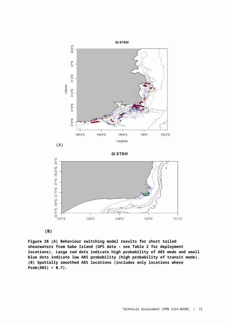
Figure 42 Spatial predictions from GAMs using ARS locations as categorized by the Behaviour switching models. See Table 2 for species and deployment location codes.
72 | Technical Assessment (PRN 1314-0450)

DRAFT CONFIDENTIAL TECHNICAL ASSESSMENT (PRN 1314-0450). DO NOT DISTRIBUTE
Figure 43 Spatial predictions from GAMs using ARS locations for AFS PTT data by colony as categorized by the Behaviour switching models. See Table 2 for species and deployment location codes.
Technical Assessment (PRN 1314-0450) | 73

5.6 GAM Diagnostics
Generally, diagnostics showed that the models did not fit well (Figure 44). Residuals of the models showed strong evidence of non-normality, however plots of observed counts as a function of predicted showed that the GAMS generally did not systematically over – or under-predict the number of locations in a given grid cell, although there were instances of large outliers which the models did not predict.
0 20 40 60 80 100
020
6010
0
AUFS
Fitted
Obs
erve
d
0 20 40 60 80 100
020
6010
0
GI_STSW
Fitted
Obs
erve
d
0 20 40 60 80 100
020
6010
0
GILP
Fitted
Obs
erve
d
0 20 40 60 80 100
020
6010
0
GR_STSW
Fitted
Obs
erve
d
0 20 40 60 80 100
020
6010
0
LBLP
Fitted
Obs
erve
d
0 20 40 60 80 100
020
6010
0
NZFS
Fitted
Obs
erve
d
0 20 40 60 80 100
020
6010
0
PD_gannet
Fitted
Obs
erve
d
0 20 40 60 80 100
020
6010
0
PE_gannet
Fitted
Obs
erve
d
0 20 40 60 80 100
020
6010
0
PTT_AUFS
Fitted
Obs
erve
d
Figure 44 Plots of observed counts in grids cells as a function of the predicted counts from the GAMs. See Table 2 for species and deployment location codes.
74 | Technical Assessment (PRN 1314-0450)

DRAFT CONFIDENTIAL TECHNICAL ASSESSMENT (PRN 1314-0450). DO NOT DISTRIBUTE
6 Diet and consumption results
6.1 Diet data collation
Data on CPFMP predator diets was collated from 24 studies of published literature from various sites in Victoria, South Australia and Tasmania (Table 6). The methodological detail in how diets were collected varied between studies with methods including scat analysis, collection of regurgitates, and DNA analysis. Sample sizes were also difficult to compare, and generally the methods employed for diet analysis, whether correction factors were applied etc., varied greatly (Figure 45).
Figure 45 Diet proportions of SPF target species (RB=redbait, JM=jack mackerel, BM=blue mackerel, AS =sardine, OT= other non-target species) by CPF species from % numerical abundance data. The study IDs are given in Table 6 and the subsequent numbers separated by an underscore indicate successive reports of diet from the same study where more than one was given. See Table 2 for species and deployment location codes.
Technical Assessment (PRN 1314-0450) | 75

Table 6 Diet proportions of SPF target species by CPF species from % numerical abundance data. The study IDs are given in Appendix 2A and the subsequent numbers separated by an underscore indicate successive reports of diet from the same study where more than one was given.
STUDY ID PREDATOR REFERENCE SITE START END REPODUCTIVE
STATUS/SAMPLING PERIOD DIET STUDY DATA TYPE
1 Little PenguinsBool et al. (2007)
Granite Island 2006 2006 Stomach contents
2 Little PenguinsBool et al. (2007)
West Island 2006 2006 Stomach contents
3 Australian Fur Seals
Kirkwood et al. (2008)
Seal Rocks 1998 2006 Monthly Scat and regurgitate
4 Australian Fur Seals
Hume et al. (2004)
Tasmanian breeding colonies and haul-outs
1994 2000 Few months of year Scat and regurgitate
5 Australian Fur Seals
Deagle et al. 2009
Seal Rocks 2007 2008 Dec-Jan Scat Hard parts and Pyrosequencing prey DNA
6 Australian Fur Seals
Deagle et al. 2009
Lady Julia Percy Island 2007 2008 Dec-Jan Scat Hard parts and Pyrosequencing
prey DNA
7 Australian Fur Seals
Deagle et al. 2009
The Skerries 2007 2008 Dec-Jan Scat Hard parts and Pyrosequencing prey DNA
8 Australian Fur Seals
Deagle et al. 2009
Combined^ 2007 2008 Dec-Jan Scat Hard parts and Pyrosequencing prey DNA
9 Australian Fur Seals
Page et al. (2005b)
Cape Gantheaume (SA) 2000 2003 Seasonal, lactating females Scat and regurgitate
76 | Technical Assessment (PRN 1314-0450)
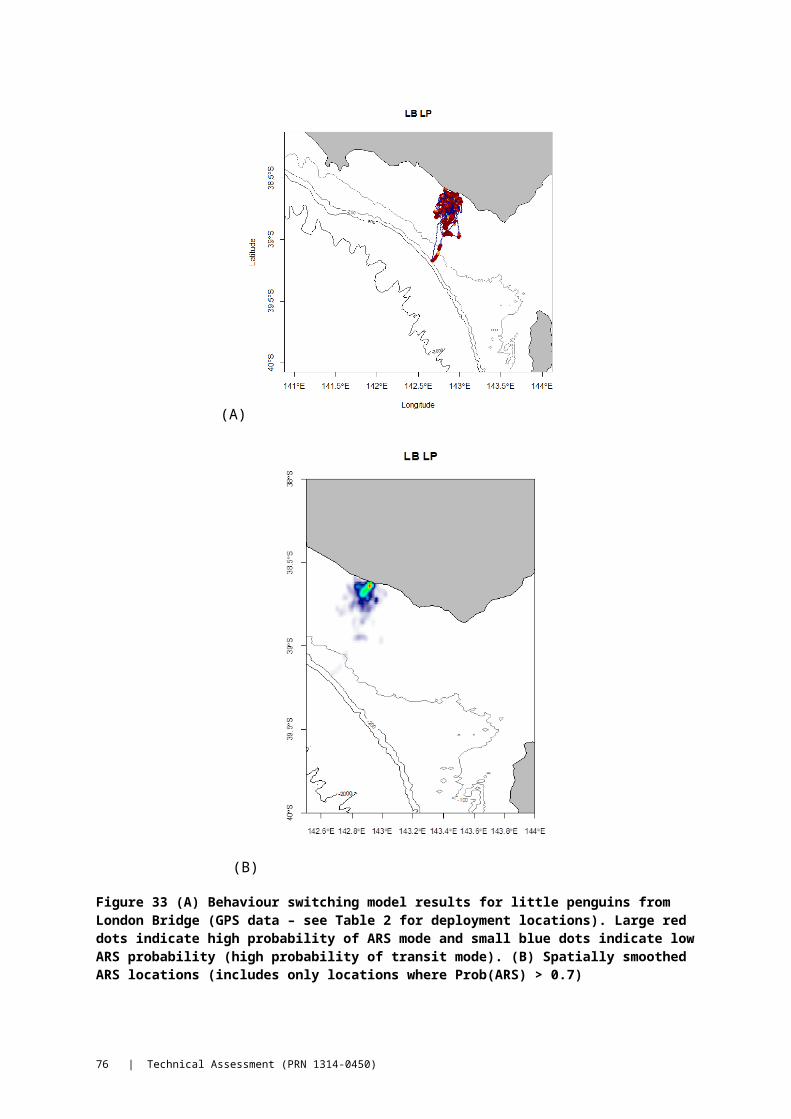
DRAFT CONFIDENTIAL TECHNICAL ASSESSMENT (PRN 1314-0450). DO NOT DISTRIBUTE
10 Australian Fur Seals
Littnan and Arnould (2007)
Kanowna Island 1997 2000 Seasonal, lactating females Scat and regurgitate
11 Australian Fur Seals
Littnan and Arnould (2007)
The Skerries 1999 2001 Seasonal, lactating females Scat and regurgitate
12 New Zealand Fur Seals
Page et al. (2005b)
Cape Gantheaume (SA) 2000 2003 Seasonal, Adult females, males,
juveniles Scat and regurgitate
13 New Zealand Fur Seals
Bool et al. (2007)
Granite and West islands (SA) 2006 2006 Non-breeding Scats
14 Australasian Gannets
Norman and Menkhorst (1995)
Port Phillip Bay 1988 1992 Throughout the year
15 Australasian Gannets Pyk et al. (2008) Pope's Eye (Port
Phillip Bay) 2002 2003 Breeding period, adults and chicks
16 Australasian Gannets Bunce (2001b) Port Phillip Bay 1997 2000 Breeding period, adults and
chicks
17 Australasian Gannets
Bunce and Norman (2000a)
Pope's Eye (Port Phillip Bay) 1998 1999 Breeding period, adults and
chicks
18 Australasian Gannets
Brothers et al. (1993)
Pedra Branca 1986 1991 Breeding period, adults and chicks
19 Shy Albatross Hedd and Gales (2001)
Albatross Island 1997 1998 Breeding adults
20 Shy Albatross Green (1974) Albatross Island 1973 1973 Nestlings
21 Short tailed Shearwaters
Montague et al. (1986)
Phillip Island 1980 1981 Breeding adults
22 Short tailed Shearwaters
Weimerskirch and Cherel (1998)
The Neck, Bruny Island 1997 1997 Adults chick rearing Short and long trips separate
Technical Assessment (PRN 1314-0450) | 77

23 Short tailed Shearwaters Skira (1986) Bruny Island and
Furneaux 1979 1980 Breeding adults
24 Short tailed Shearwaters
Connan Maëlle (2010)
The Neck, Bruny Island 1997 1997 Breeding adults
78 | Technical Assessment (PRN 1314-0450)

The data also indicated that there is no way to characterize a single diet for each species. Simple averaging of the proportion of prey species in the diet leads to unrepresentative estimates with extremely high uncertainty, with extremely high uncertainty with very large standard deviations around the mean diet proportion of target species (Table 7). This could be due to a combination of biological factors, such as regional variation in diet, prey switching, etc., as well as due to differences in observational characteristics of each study (e.g. sample size, method of diet characterization, etc).
These results point to risks if single estimates of diet are used for estimates of consumption. Or put another way, it would be reasonable to look at the implications of using the results of different diet studies to examine the degree to which this influences consumption results. The goal in terms of the management context is to bound estimates of consumption sufficiently robustly that estimates of predator requirements are not biased low. Accordingly in the consumption modelling described below we chose diet proportion estimates where SPF target species were a significant part of the diet.
Table 7 Means and standard deviations for diet proportions from the studies listed in Table 6. The standard deviations are very large relative to the mean proportion indicating a large degree of variability in the mean diet proportion between studies. LP = little penguin, AFS = Australian fur seal, NZFS = New Zealand fur seal, GAN = Australasian gannet, SHYA = shy albatross, STSW = short tailed shearwater.
LP AFS NFS GAN SHYA STSW
Prey Mean SD Mean SD Mean SD Mean SD Mean SD Mean SD
Redbait 0.01 1.41 0.31 0.71 0.13 0.77 0.19 1.66 0.02 1.25 0.04 1.77
Other species 0.93 0.04 0.49 0.51 0.86 0.13 0.54 0.51 0.91 0.12 0.85 0.29
jack mackerel 0.0 - 0.20 0.76 0.01 1.00 0.06 0.64 0.03 0.59 0.04 1.77
blue mackerel 0.0045 1.41 0.02 2.79 0.001 2.00 0.04 0.72 0.02 1.73 0.04 1.77
sardine 0.06 0.24 0.01 2.06 0.004 1.21 0.20 1.32 0.02 1.73 0.04 1.77
6.2 Biomass consumption calculations
Despite numerous studies being published on the diet of central place foraging predators in the SPF, few have reported data useable for prey biomass consumption, referring mainly only to frequency of occurrence and/or numerical abundance. Information on prey size is lacking for most of them. Therefore, in the present study, spatial prey biomass consumption was calculated from reports that specifically listed proportional mass contribution of various prey to the diet.
For Australian fur seals, diet data were obtained for adult females from (Arnould and Kirkwood 2008) and body mass (76 kg) from Arnould and Warneke (Arnould and Warneke 2002). For New Zealand fur seals, diet data were obtained from Page et al. (Page et al. 2005a) and adult female body mass (42 kg) from (Page et al. 2005a). The gross energy composition of prey was assumed to be 4.98 MJ·kg-1 for fish, 3.65 MJ·kg-1 for cephalopods, and 8.90 MJ·kg-1 for birds (Goldsworthy et al. 2003, Einoder et al. 2013a). Daily energy expenditure value was calculated for both species (39.8 MJ·day-1 and 26.8 MJ·day-1, respectively) from a mass-specific allometric relationship following the approach of Goldsworthy et al. (Goldsworthy et al. 2003). While fur seals provisioning pups alternate foraging at sea with fasting on land to nurse their pup, a constant daily metabolic rate was assumed for the duration of the pup-rearing period as all body reserves metabolized on land must be acquired during trips to seas. As per Goldsworthy et al. (Goldsworthy et al. 2003), an assimilation efficiency of 80% was used to convert daily energy expenditure into biomass consumption estimates.
For Australasian gannets, diet data were obtained from Pyk et al. (2013). Body mass was assumed to be 2.6 kg (Angel and Arnould in press) and daily energy expenditure as 2.203 MJ·day-1 (Green et al. 2013). For short tailed shearwaters, diet data were obtained from Einoder et al. (Einoder et al. 2013a), body mass was
Technical Assessment (PRN 1314-0450) | 79

assumed to be 0.62 kg (Einoder et al. 2008) and daily energy expenditure was estimated as 0.943 MJ·day-1 from data on streaked shearwaters (Calonectris leucomelas). Diet data for little penguins was obtained from (Chiaradia et al. 2010). Body mass was assumed to be 1.0 kg (Green et al. 2008) and daily energy expenditure as 1 MJ·day-1 (Costa et al. 1986). The gross energy composition of prey was assumed to be 4.68 MJ·kg-1 for fish, 3.65 MJ·kg-1 for cephalopods, and 3.3 MJ·kg-1 for krill (Einoder et al. 2013a).
6.3 Caveats and biological uncertainties associated with diet and consumption characterization
Accurate prey biomass consumption estimates for predators are inherently difficult to obtain, especially for marine vertebrates, where direct observations of feeding are not possible. In addition to the large number of known biases in seabird and pinniped diet reconstruction techniques (Staniland 2002, Arim and Naya 2003, Tollit et al. 2006), there is substantial temporal and geographical variability in the species and size classes of prey consumed (see Appendix 2A). The prey biomass contribution data used in the present study, therefore, may not reflect this variability. Secondly, the values for prey gross energy composition used in the present study were derived from small samples sizes in previous studies and may not be representative across the geographic range of the tracking data. Thirdly, obtaining accurate data on daily energy expenditure in free ranging animals is difficult and for most species where data are available these come from a single study, limiting analysis of temporal variability and influence of environmental factors. Generally, studies of captive animals are required to estimate correction factors which account biases due to for digestion of otoliths, errors in estimating the number of hard parts, amongst other biases (Grellier and Hammond 2006).
In the present study, estimates of daily energy expenditure for fur seals were derived from a mass-specific allometric relationship derived from other otariid species (Goldsworthy et al. 2003) and, hence, this may lead to under- or over-estimation of prey consumption. Similarly, no data were available for the short tailed shearwater and so estimates from another similar-sized shearwater (n = 3) was used and, while data were available for little penguins and Australasian gannets, these were each from single studies and small sample sizes (2 and 8, respectively). Furthermore, the coefficient of assimilation (80%) of prey gross energy is likely to be influenced by prey composition (i.e. fat to protein ratio), meals size and the physiological condition of the predator (Rosen et al. 2000). Mean body mass of predator species is also likely to vary temporally in relation to stage of breeding and environmental conditions. Finally, the estimates of prey consumption presented in this study for birds is based upon adult daily energy expenditure and does not account for the additional consumption required for provisioning of chicks. Hence, all these uncertainties will influence the accuracy of the spatial estimates of consumption by these predators of SPF target species.
80 | Technical Assessment (PRN 1314-0450)

7 Population Consumption models
The general form of the spatial consumption equation used here is as follows:
φ ijk=N i ηij ξ i π ik f (n jk , ϑ j ) , (5)
where:
N i: spatially aggregated abundance of predator i ηij: preference for prey species j for predator i ξ i: maximum consumption rate of predator i π ik: proportion of abundance of predator i in location k n jk: density of prey species j in location k f (∘ ): predation response function to changing prey abundance ϑ j: parameters of the predation response function
While this is a somewhat idealised version of how predators consume their prey, it is general enough for the processes we wish to explore and the kind of data available. For the sake of simplicity we have avoided explicitly including any kind of time variable, though it is simple to do if required. It also extends naturally to a spatially aggregated (e.g. across a full species ``range'' however defined) consumption estimate:
φ ij=N iηij ξ i∑k
π ik f (n jk ,ϑ j ). (6)
For the estimates shown here we restricted the consumption period to the number of days in the year that animals are actively feeding young. Therefore all estimates of consumption presented here are for breeding females in the case pinnipeds and for seabirds incubating or feeding chicks. Table 8 shows the estimates of breeding duration and daily maintenance biomass consumption used for the model. The diet studies selected for use in consumption modelling are given in Table 9. In our calculations we combined the various estimates of proportion of SPF target species in the diet into a single figure. Note how SPF target species were lumped together although species specific estimates could be derived similarly.
Table 8 Figures for daily maintenance ration from percentage biomass diet studies and estimates of metabolic rate and also the duration of breeding period (all consumption estimates are restricted to breeding period and for breeding adults only). AFS = Australian fur seal, NZFS = New Zealand fur seal, LP = little penguin, STSW = short tailed shearwater, GAN = Australasian gannet.
PREDATOR SPECIES MAINTENANCE BIOMASS INTAKE (KG)
DURATION OF BREEDING (DAYS)
AFS 10.26 300
NZFS 6.96 300
LP 0.28 126
STSW 0.31 37.5
GAN 0.59 144
Technical Assessment (PRN 1314-0450) | 81
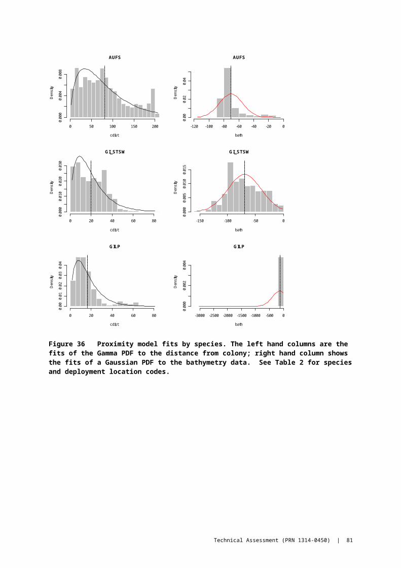
Table 9 Sources of SPF diet proportion and the estimated proportion for each CPFMP species. The study ID code links to Appendix 2 (diet data) and is also indicated on Figure 36. AFS = Australian fur seal, STSW = short tailed shearwater, GAN = Australasian gannet, NZFS = New Zealand fur seal, SHYA = shy albatross, LP = little penguin.
SPECIES STUDYID/REFERENCE) PROPORTION OF SPF SPECIES IN DIET
AFS 3_1, Kirkwood et al. 2008 0.65
6_1, Deagle et al. 2009 0.84
STSW 21_1, Montague et al. 1986 0.16
GAN 14_1, Norman & Menkhorst, 1995 0.604
18_1, Brothers, 1993 0.876
NZFS 12_1, Page et al. 2005 0.25
SHYA 19_1, Hedd & Gales, 2001 0.09
LP 2_1, Bool et al. 2007 0.07
7.1 Predation response function
The specific functional form relating predator consumption rates to prey density, and the parameters therein, is notoriously difficult to estimate and can take many forms (Plagányi 2007). However, it stands to reason that predator consumption is not independent of prey abundance, and it would be unwise to ignore functional response relationships altogether.
To demonstrate the importance of the functional response when considering consumption estimates, we employ the simple Holling response function (Holling 1965):
f (n jk , μ j )=n jk
ν
n jkν +μ j
ν , (7)
where the key parameters are: μ, which denotes the half-saturation (prey density at which the predation rate is reduced to 50% of the maximum), and ν, which controls the rate at which the curve asymptotes towards 1 as prey density increases. What is most important is the way the half-saturation scales relative to prey density, not the units and - purely as an example - we assume ν=2 (Type III response). In terms of indicative scenarios for both n jk and μ we considered the following (illustrated in Figure 46):
1. Weak/medium/strong predation uptake responses (see Figure 46) with μ=0.1 ,0.25 , 0.5 and assuming the units of n jkto be relative to the unfished state (i.e. ∈[0,1])
2. Two potential prey abundance states with n jk=0.5 ,0.8 - the first state represents something “close” to the Maximum Economic Yield (MEY) target of ca. 48% as defined in the Commonwealth Harvest Strategy policy (here we are assuming an actual estimate does not currently exist) , and the second is assumes that the prey population is relatively lightly fished at 80% unfished biomass.
3. For a CV for the prey density we assumed a simple 25% CV as, at least from the single- species population assessment viewpoint, this would represent an acceptable level of precision from which to estimate trends in the associated population.
82 | Technical Assessment (PRN 1314-0450)

Figure 46 The functional response curves under scenarios of weak/medium/strong predation uptake responses (with μ=0.1 ,0.25 , 0.5 respectively).
7.2 Uncertainty calculations
Clearly, defining even a fairly simple spatial prey consumption equation requires the use of several quantities (i.e. the terms in equation 6), each of which will have to be estimated from data and therefore will carry an associated level of uncertainty. In a management setting where decision makers need to know the degree of certainty around the final estimates of prey consumption by predators.
In this section we outline an approach to estimating the uncertainty in spatial consumption given the individual variances of the constituent variables used in the calculation.
The delta method (Oehlert 1992) is a relatively simple approach to calculating the variance of a given variable, which is itself a function of several other variables. The assumption on the input variables is that they are (statistically) well estimated and asymptotically normally distributed. To outline the general calculation it is useful to define the consumption φ to be a function g (θ ), where θ is a vector containing all the variables that define the consumption. Assuming we can define the covariance matrix of θ̂ (the estimates), Σ, then the approximate variance of φ, given this covariance matrix, is
V (θ̂ )≈( ∂ g∂θ )
T
⋅Σ ⋅( ∂ g∂θ ), (8)
where, T denotes vector transpose and the gradients are evaluated at θ=θ̂. With a spatially aggregated version it is clear from (2) that the correlation between predator and prey spatial abundance needs to be accounted for, if we are not going to over-estimate the overall CV in consumption by assuming spatial independence.
For the particular variables of interest in the consumption equation, some will have actual variance estimates for (spatial distribution), some we can construct variance estimates for from the data (diet preference), and for others we can run scenarios if variance estimates are unavailable. In particular, for the prey preference parameter the following approach was used:
For a given predator i, a diet study can provide both an estimate of the SPF species j (or single species if required) in the diet, pij, and the sample size of the diet data used to estimate that proportion, N p. By assuming a binomial distribution for the number of prey samples found in the predator’s diet, and
Technical Assessment (PRN 1314-0450) | 83

assuming a non-informative beta distribution – Beta (0.5,0 .5 ) - for the true proportion of prey group j in the diet, the posterior distribution of the prey preference will be:
P (ηij∨… )=Beta (0.5+ pij N p ,0.5+ (1−pij )N p ), (8)
and so an appropriate variance estimate is directly calculable that reflects the level of sampling effort in the diet study.
84 | Technical Assessment (PRN 1314-0450)

8 Consumption model results
Because of the pilot nature of this study, the uncertainties in various data sources, we compiled non-spatial consumption estimates (i.e. for the entire range of the diet and abundance data) and provided some example of spatial consumption calculations based on hypothetical spatial areas of interest. These demonstrate the possibility of combining the spatial models and associated uncertainty in the predictions.
8.1 Non-spatial consumption estimates
Estimates of consumption for all SPF target species combined over the entire CPFMP abundance dataset (i.e. across all colonies), was calculated using the methods outlined in the previous section. In these calculations the proportion of the predator population within the region, π ik=1. Scenarios for functional response, prey biomass relative to unfished were followed as per those outlined in the previous section.
In these we chose data from eight studies to determine the proportion of SPF target species in the diet (Table 9). These were not the total of available diet data, but for the sake of illustration, were selected from studies that indicated the highest possible proportion of SPF target species in the predators’ diet.
The results of these are shown in Figure 47 with a summary of average and range of calculations given in Table 10. For these inputs, the results show that Australian fur seal are expected to be the largest consumers of SPF target species, followed by short tailed shearwater (despite relatively low prevalence of SPF target species in their diet), then New Zealand fur seal, gannets, little penguins and shy albatross, respectively. The seabirds generally target krill species (see Appendix 2) and the ranking of short tailed shearwater as the second highest consumer of SPF prey is due to the relatively high number of individuals in the SPF for this species. Again, the assumptions about residency within the SPF may be influential in this calculation and should be kept in mind.
Table 10 Mean, minimum, maximum tonnage of consumption of SPF target species by each of the CPFMP species from the non-spatial consumption estimates given in Figure 34 above. AFS = Australian fur seal, GAN = Australasian gannet, LP = little penguin, NZFS = New Zealand fur seal, SHYA = shy albatross, STSW = short tailed shearwater.
SPECIES CONSUMTPION (TONNES)
Mean Min Max
AFS 88446.6 47828.8 120179.6
GAN 1011.7 508.6 1449.8
LP 970.3 596.1 1175.7
NFS 9441.2 5813.6 11440.5
SHYA 17.5 10.8 21.2
STSW 31817.9 19528.8 38710.3
Technical Assessment (PRN 1314-0450) | 85

AFS N (x1000): 47.8 (CV: 0.0084 )
Scenario
Con
sum
ptio
n (1
000'
s t)
MEY MEY MEY B_0 B_0 B_0 MEY MEY MEY B_0 B_0 B_0
6080
100
120
3_1
3_1
3_1
3_1
3_1
3_1
6_1
6_1
6_1
6_1
6_1
6_1
0.0
0.1
0.2
0.3
0.4
0.5
0.6
0.7
CV
GAN N (x1000): 19.8 (CV: 0.05 )
Scenario
MEY MEY MEY B_0 B_0 B_0 MEY MEY MEY B_0 B_0 B_0
0.6
0.8
1.0
1.2
1.4
14_1
14_1
14_1
14_114_1
14_1
18_1
18_1
18_1
18_1
18_1
18_1
0.0
0.1
0.2
0.3
0.4
0.5
0.6
0.7
CV
LP N (x1000): 483 (CV: 0.03 )
Scenario
MEY MEY MEY B_0 B_0 B_0
0.6
0.7
0.8
0.9
1.0
1.1
2_1
2_1
2_1
2_1
2_1
2_1
0.0
0.1
0.2
0.3
0.4
0.5
0.6
0.7
CV
NFS N (x1000): 22.3 (CV: 0.017 )
Scenario
Con
sum
ptio
n (1
000'
s t)
MEY MEY MEY B_0 B_0 B_0
67
89
1011
12_1
12_1
12_1
12_1
12_1
12_1
0.0
0.1
0.2
0.3
0.4
0.5
0.6
0.7
CV
SHYA N (x1000): 14.8 (CV: 0.58 )
Scenario
MEY MEY MEY B_0 B_0 B_0
0.01
20.
014
0.01
60.
018
0.02
0 19_1
19_1
19_1
19_1
19_1
19_1
0.0
0.1
0.2
0.3
0.4
0.5
0.6
0.7
CV
STSW N (x1000): 20920 (CV: 0.12 )
Scenario
MEY MEY MEY B_0 B_0 B_0
2025
3035
21_1
21_1
21_1
21_1
21_1
21_1
0.0
0.1
0.2
0.3
0.4
0.5
0.6
0.7
CV
Figure 47 Total estimates of SPF target species consumption for total breeding adult CPFMP populations (see text for definition). The coloured bars give the consumption according to the scenarios outlined in section above (Scenarios labelled “MEY” indicates a prey abundance of 0.5 × B0 and “B_0” indicates a relatively unfished prey biomass of 0.8 × B0. Grey bars give the estimated CV given the scenario. AFS = Australian fur seal, GAN = Australasian gannet, LP = little penguin, NZFS = New Zealand fur seal, SHYA = shy albatross, STSW = short tailed shearwater.
86 | Technical Assessment (PRN 1314-0450)

8.2 Example of spatial consumption by area estimation
As an example of how these models can be used to calculate spatial consumption at the level of a management unit, we arbitrarily chose the data from Australasian gannets and Australian fur seals as examples. The GAMs (Figure 42) fitted to data from Point Danger and Kanowna Island for gannets and fur seals were used to make predictions of the spatial distribution of individuals from other colonies. Five spatial blocks were constructed, again, these were chosen arbitrarily as a demonstration of the approach (
). For this example, we chose a weak functional response (μ =0.1), a relatively lightly depleted prey stock (0.8 B0). Uncertainty on gannet colony counts was unavailable (see Appendix 1), so we assumed a low CV of 5%. SPF diet proportion came from the study listed as 18_1 (Norman and Menkhorst 1995) as outlined in Table 9. For the fur seals we again selected a weak functional response scenario and lightly depleted prey stock. The CVs on colony abundance for Australian fur seal were all low (1-10%- see Appendix 1).
The estimates of consumption (Table 11) predicted that for gannets, area 1 would be responsible for approximately half (49%) of the consumption across all areas (1-5); area 5 was predicted to account for 21% of the consumption with areas 2 and 4 being similar at 12% and 11% respectively. Area 3 accounted for only 6% (Table 11). For Australian fur seal, 30% was expected to come from the western region (area 1), 32% from area 5, areas 2, 3 and 5 made up the remaining 39%. These results showed apparently low levels of uncertainty (all around 10% - see Table 11). We expect that these are likely to be considerably underestimated due to the aforementioned, and likely similar underestimates of uncertainty in the spatial model calculations. Obviously the spatial blocks considered here and the scenario parameters may be totally unrepresentative of the actual state of the SPF. However, the demonstration shows how consumption and uncertainty can be obtained and could be deployed in actual management scenarios.
Figure 48 Hypothetical spatial areas used for spatial consumption estimation, along with the locations of Australasian gannets (GAN) and Australian fur seal (AFS) used in the consumption modelling. Consumption estimates are given in Table 10.
Technical Assessment (PRN 1314-0450) | 87

Table 11 Estimates of consumption for hypothetical spatial areas shown in
for (A) Australasian gannets and (B) Australian fur seals. Also shown are the CVs on consumption estimates, the estimated number of individual predators using each area according to combined predictions from the colonies shown in
.
(A) AUSTRALASIAN GANNETSDIET STUDY 18(1)
AREA
1 2 3 4 5 TOTAL
Consumption (tonnes) 379.38 96.79 49.02 89.41 164.27 778.87
CV 11% 12% 12% 12% 12%
N 7464.11 1943.86 982.88 1802.50 3145.49 15338.83615
Survey population 19808 percent of population 77%
(B) AUSTRALIAN FUR SEALSDIET STUDY 3(1)
AREA
1 2 3 4 5 TOTAL
Consumption (tonnes) 26414.71 11480.16 7900.42
28326.51 15138.40 89260.2
CV 10% 11% 10% 10% 10%
N 13766.85 5951.20 4105.83
14685.12 7931.63 46440.6
Survey population 23793 percent of population 98%
88 | Technical Assessment (PRN 1314-0450)

9 Characterization of predator vulnerability
As central place foragers, the marine predators discussed in this report (seals and seabirds) are constrained to foraging within certain distances of their breeding colonies throughout certain periods of the annual cycle. When chicks and pups are young, the need for regular trips to feed young is greatest and consequently adults are limited in their ability to forage further afield. These key reproductive periods vary across the six species (see Table 12). One universally important period (high vulnerability) across species is mid/late spring to early summer. At this time most species are incubating, feeding young chicks/pups, or gathering reserves to recoup body reserves prior to pupping and lactation.
Table 12 Timing of breeding and offspring growth for little penguins, short-tailed shearwaters, Australasian gannets, and Australian and New Zealand fur seals within the SPF fishery area (grey). Months denoted in dark grey depict timing of greatest vulnerability when offspring are being incubated/gestating or are very young.
COMMON NAME FORAGING BEHAVIOUR J F M A M J J A S 0 N D
Little penguin Pelagic
Australasian gannet Plunge dive
NZ fur seal Pelagic
Australian fur seal Benthic
Short-tailed shearwater Plunge dive
Shy albatross Surface feeder
Information regarding the movements of the five predator species during the non-breeding phase of the annual cycle for adults is more scant. Although not constrained by breeding and the need to regularly provision young, as discussed above, the requirements for prey consumption and corresponding post-breeding improvements in body condition are likely to be important for adults to gain condition which can be invested in the following breeding seasons’ young.
All seabirds and females of fur seal/sea lion species are central place foragers during the offspring rearing period, having to return to the natal colony regularly to provision their young. During this period they are vulnerable to the negative effects of reductions in food availability as they are limited in the amount of time they can forage by the fasting endurance of their young.
For Australian fur seals and New Zealand fur seals, this corresponds to ~10 months from when pups are born (Nov/Dec) until they are weaned (Oct). However, the foraging period between the end of lactation and the birth of the next pup (i.e. the third trimester of active gestation) is important as the resources the female can acquire during this short period can determine the size of the pup and greatly influence its early post-partum survival. Unhindered by having to return to land to nurse a pup, adult females have been shown to disperse further from the colony during this period in search of resources (Arnould and Hindell 2001, Hoskins et al. 2008).
Short tailed shearwaters foraging locally during the pre-laying period Sept-Oct before foraging in the Southern Ocean in preparation for egg laying. Thereafter, they alternate short local foraging trips for chick-provisioning with long self-maintenance trips to the Antarctic waters until they depart on the winter migration in mid-April. Hence, significant local reductions in food supply during the summer months could have negative impacts on offspring provisioning rates and fledging success. However, breeding success is likely to be also influenced by variations in food availability in the Southern Ocean during this period. As the species undertakes a winter migration to the North Pacific, it is not affected by food availability in south eastern Australia during this period. Nonetheless, environmental variability in the region during winter could have effects that impact prey availability in the subsequent summer breeding period.
Technical Assessment (PRN 1314-0450) | 89
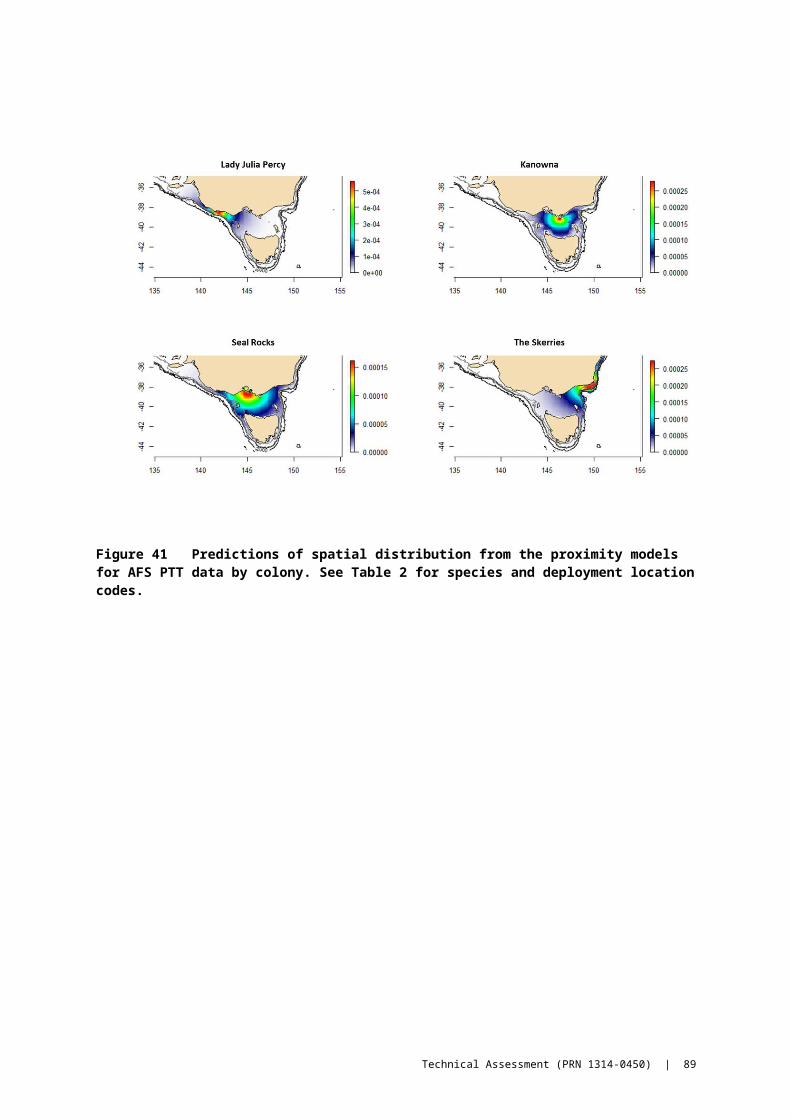
While little penguins are restricted in their foraging range during the breeding season, the few studies that have investigated their winter non-breeding distribution suggest populations within Bass Strait generally continue to forage in the same areas. Satellite tracking of little penguins from Phillip Island during winter found most individuals (72%) undertook single-day foraging trips, with most of the remainder travelling into Port Phillip Bay over several days (McCutcheon et al. 2011). Similarly, while Australasian gannets in Bass Strait have been shown to be restricted in their foraging range to the continental shelf areas during the breeding season, preliminary results suggest these populations also do not venture far during the winter non-breeding period. Over-winter tracking of individuals from Pope’s Eye (A. Bunce, unpublished data) indicated birds spent the majority of the time on the continental shelf in western Bass Strait. Assuming individuals from other colonies in Bass Strait behave the same during the non-breeding period, they are likely to be impacted in a similar way to local food restrictions at this time as during the breeding season. Indeed, studies have shown survivorship in seabirds is lowest during the winter non-breeding period (Harris et al. 2010, Tranquilla et al. 2010).
The estimates of biomass consumption presented in this study are limited to individuals raising offspring as this is the proportion of the adult population restricted in their range as central place foragers and are likely to be the most crucial to population viability. However, potential impacts of non-predator prey exploitation (i.e. fisheries) will be experienced by all components of a predator population that forages in the same region. While New Zealand fur seals have been shown to segregate by sex and age, with males and juveniles foraging further from colonies and beyond the continental shelf edge (Baylis et al. 2008, Baylis et al. 2012), all segments of the Australian fur seal population feed almost exclusively on the shallow continental (Arnould and Kirkwood 2008, Arnould et al. Unpubl. data, Kirkwood Unpubl data). Hence, for the latter, the whole population may be subject to impacts of prey depletion by commercial fisheries in the region. Similarly, little penguins are mainly forage <50 km from coasts and, therefore, non-breeding individuals are likely to exploit the same resources as adults provisioning chicks. The distribution of non-breeding Australasian gannets in Australia is not known but studies of New Zealand individuals indicate that post-fledging birds may roam great distances, including to the Australian coastal areas (Ismar et al. 2010, Ismar et al. 2011).
Due to restraints on time and availability of data, especially for seabirds, this report has been unable to consider estimates of entire population’s consumption, i.e. for all ages and for pinnipeds, for both sexes. As a result the estimates of consumption (Table 10 and Figure 47 ) are expected to be only a small proportion of the entire population. To estimate consumption of the entire population would require several data inputs which were not feasible to compile given the constraints of this study:
- The population age or stage distribution- Mass-specific maximum consumption- Spatial estimates of consumption would require representative tracking data for representative
ages/stages and sexes. - Indications of whether prey preference or proportion changes with age or size.
The age structure of pinniped populations is available, but only in certain colonies, but is very poorly known in short-tailed shearwaters, Australasian gannets and most little penguin colonies.
90 | Technical Assessment (PRN 1314-0450)
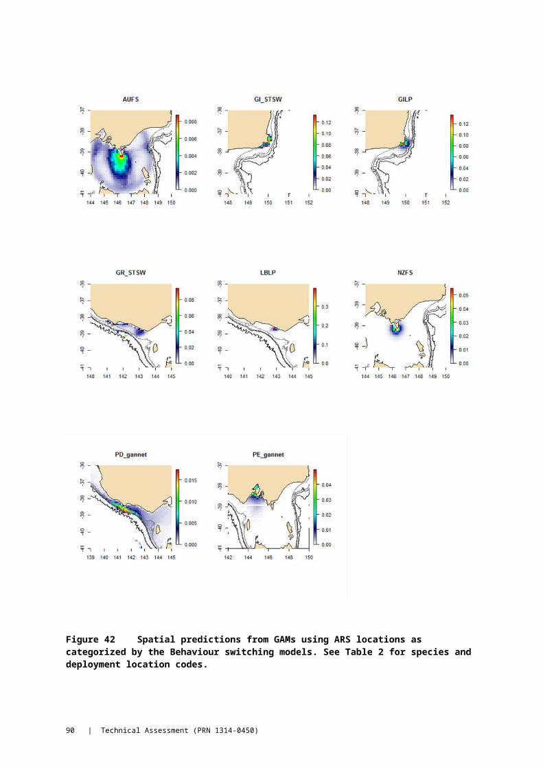
10 Potential spatial management measures to reduce the risk of local depletion of prey species by fishing
There is a range of management approaches that could be employed to reduce the probability of local depletion of prey populations and the potential follow on consequences for CPFMP populations within the SPF. These include approaches that are and are not explicitly spatial in their implementation. This section outlines the general forms of spatial and non-spatial management measures that could be considered for the SPF and the logic that underpins them. It is followed by a section on Management Strategy Evaluation (MSE). The latter provides an overview of the MSE approach, its potential advantages in the context of the design and evaluation of measures to minimize the risks associated with local depletion of prey species, and an outline of the technical and consultative steps associated with undertaking such an approach.
We consider that the following four categories of spatial management options are relevant to minimizing the potential risks associated with local depletion of population of important prey species in the SPF:
(1) Setting TACs that account for CPFMP foraging requirements: In this case, the TAC set for the fishery would account for predation of CPFMP populations on SPF target species in such a way that the required abundance of prey for the CPFMP populations should be available to them. This is not a spatial management option but is worthy of consideration as, depending on the extent of spatial overlap between harvesting rates of the SPF, patterns of predation by CPFMP and mixing and connectivity between prey populations, explicit spatial management of the distribution of fishing effort and/or catch may not be required to mitigate probability and impacts of local depletion.
(2) Spatial allocation of TAC: The intent of this option would be to reduce the potential for local depletion and, in doing so, increase the probability that the necessary abundance of prey is available to the populations of CPFMP. In this class of strategy, the fishery would be split into a number of spatial areas, each of which may have an area specific TAC associated with it. The area specific TACs might be weighted according to the abundance of CPFMP within these blocks, estimated prey density, by the expected level of effort, or some other relevant criterion.
(3) Spatial closures: This class includes spatio-temporal closures around breeding colonies during the breeding season. These may be designed to include the entirety of the land-based breeding cycle, or some component of it, as it seems precautionary to consider these especially around peak periods of provision of food to young. The spatial extent of the closure(s) could be related to foraging ranges or spatial models of at sea distribution. Both the spatial and temporal extents of the closure associated with this form of measure are likely to vary among species and possibly populations.
(4) Move-on rules: This category involves specifying a rule that only a certain percentage, or absolute amount, of catch can be taken within a particular spatial block within a certain period. Move on rules are event-triggered strategies that effectively result in a temporary closure of part of a fishery when a catch or bycatch threshold is reached. These have been employed in a variety of fisheries often for protection of vulnerable marine ecosystems, and often in the context of protecting benthic communities from trawling impacts (Auster et al. 2011, Dunn et al. 2014) or in mitigation of bycatch (CCAMLR 2011). In the current setting of the SPF, such a rule might stipulate that within a particular area, no more than a given percentage of the tonnage of SPF species could be taken over
Technical Assessment (PRN 1314-0450) | 91
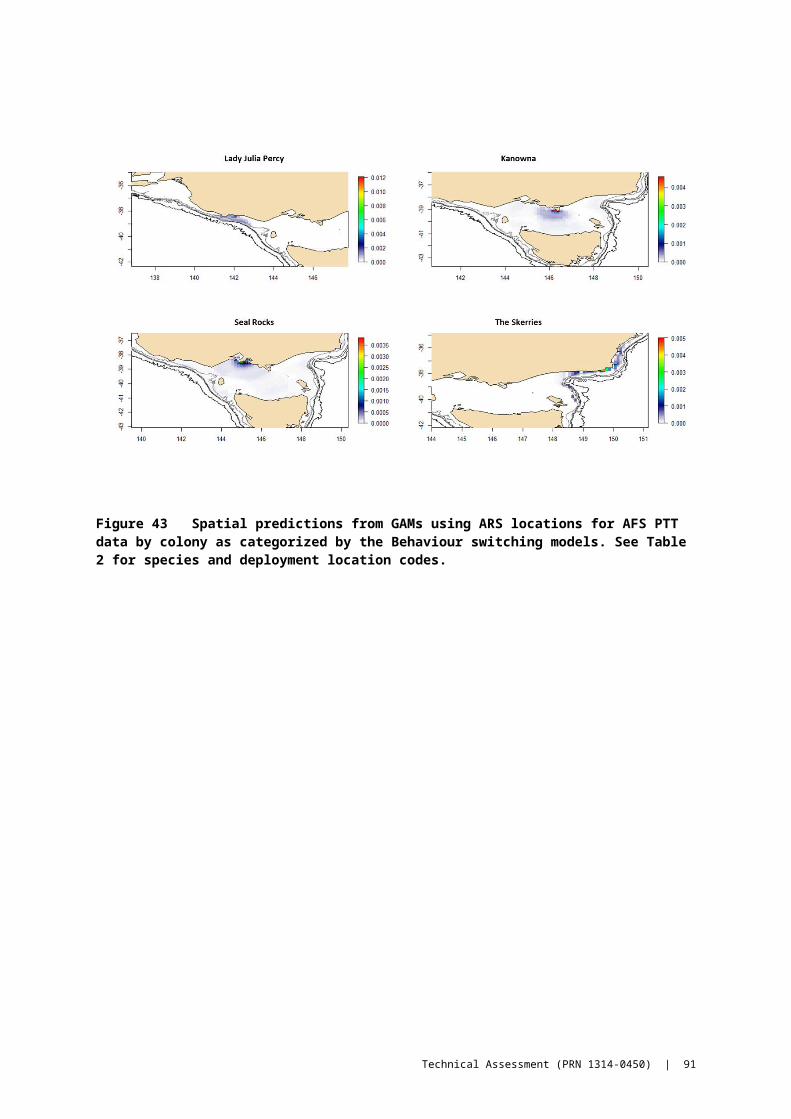
the peak summer breeding periods of CPFMP. The aim of this measure is to reduce the local intensity of fishing and thereby mitigate the risk of location depletion of prey, especially at periods of peak vulnerability, such as within the breeding season.
Within these four general types of management measures, there are many possible permutations of closures, allocation of catch and design of move-on-rules; each full specified permutation (i.e. specific period of closure, quantity of allowance for predators, spatial extent of closure, amount catch/percentage of TAC triggering move-on rule) constitutes an individual management strategy.
In considering spatial management measures (classes 2-4) it is important to determine, from an effectiveness and efficiency perspective, whether these spatial explicit management measures offer any advantage over non-spatially explicit measures (1, and potential forms of 4). The limitations of this project preclude a full quantitative investigation of these issues. Further, the data and modeling gaps in the previous sections of this report mean our present ability to design and assess the specific impacts and likely success of any particular spatial management strategy for the majority of the area covered by the SPF are limited.
There are areas of the SPF, however, that are relatively well-studied, such as South Australia (Goldsworthy et al. 2013) and, to a lesser extent, Bass Strait waters (this report). In these regions there may be scope for direct use of the available movement, foraging and diet data for some CPFMP species, in the design and evaluation of practically implementable spatial management strategies to minimize the potential risks to populations of local depletion by the SPF. Outside these regions, however, the CPFMP populations are generally poorly monitored and observed in terms of predator diet, abundance and at-sea distribution. For the reasons identified earlier (section) there are challenges for extrapolating the at-sea distribution models developed for those regions where there are sufficient data to those where there is not. Accordingly, given the large range of potential permutations for specific spatial management regimes in any particular region and the large uncertainty in many of the important foraging and population dynamics processes, we recommend the use of Management Strategy Evaluation to evaluate the potential effectiveness of alternative forms of spatial management and identify general features that contribute to making a strategy robust to the range of forms of uncertainty. The MSE process also has the advantage of directly identifying the types of research and monitoring that can most cost-effectively address the current uncertainties in understanding and future monitoring the status of the system of interest.
Management Strategy Evaluation (MSE – see section 11.2 for a detailed overview) testing could be used to compare the performance of closures with different timing, size and location. This could be similar to the approach recently adopted by CCAMLR where alternative spatial allocation models were compared based on (1) historical catch within the Small Scale Management Units, (2) estimated predator consumption in the SSMU; (3) estimated standing stock of krill in the SSMU; and (4) standing stock, less annual predator demand in the SSMU.
In the SPF, some of these data are available in some regions. While not spatially complete, these types of regional estimates could be obtained for the areas that have good data and an MSE approach would be useful because it could take account of the uncertainties in the data. The CCAMLR approach also included an option with feedback, where the spatial allocation would be adjusted periodically based on monitoring data, so this would be a useful option for the SPF if sufficient monitoring exists (see Section 11). This demonstrated that management options which reduced coastal fishing relative to oceanic fishing reduced risks to both the fishery and the ecosystem.
Different management strategies are likely to be required for predators with different movements. Our analysis of percentage of categorized foraging effort (section 5.4, Figure 34) within a radius of a home-colony is, in a very preliminary sense, qualitatively useful, in this regard. Again we note that in particular, the short-tailed shearwaters and New Zealand fur seals data comprised extremely low sample sizes, and most species were subject to limitations in terms of the spatial coverage of colonies from which tags were deployed. However, based on the these initial results, along with movement studies elsewhere (Kirkwood and Arnould 2012, Goldsworthy et al. 2013), it may be that wide ranging species such as New Zealand and
92 | Technical Assessment (PRN 1314-0450)

Australian fur seals might be sensitive to the overall level of fishing effort rather than spatial concentration of fishing effort near colonies. Conversely, species which are highly spatially constrained in their foraging, such as little penguins might be more at risk from fishing relatively close to their colonies. A complication to this is that, depending on prey movements and density, harvesting of prey outside the foraging range of highly spatially constrained predators may still impinge on their access to prey if the fishery is “upstream” of the foraging zone. This highlights the need to integrate prey survey data into spatial analyses of predator foraging.
Again, the scenarios listed above could be tested using MSE which we expand upon below. We note that a key sensitivity in any such analyses would be the rate of movement of the prey and in particular the rate at which prey are replenished in a region due to movement of forage fish. If there are no reliable estimates of small pelagic fish movement, it might then be necessary to test the most conservative option, namely, that prey does not move.
Technical Assessment (PRN 1314-0450) | 93

11 Future Research and monitoring needs
Given our appraisal of the current state of knowledge of abundance, diet, and spatial distribution of CPFMP in the SPF we now outline priorities for further research. Our approach is has two components (1) integrated monitoring to address regional gaps in basic biology and (2) a management strategy evaluation exercise to perform (i) a short-term, tactical assessment of possible spatial management options (outlined below) and (ii) a statistical design study to optimize the monitoring. This aims to maximize the likelihood of any monitoring program delivering a sufficiently clear signal in predator responses to fisheries activity so that management responses are based on the best possible information. Our general proposed approach is along the lines of the CEMP used for the Antarctic by CCAMLR (CCAMLR 2014 ).
11.1 Recommendations for monitoring and further data collection:
This report has noted some large regional gaps in our understanding of CPFMP diet, abundance and spatial distribution at sea. Outside of the research conducted in South Australia and Victoria, there is little consistent monitoring of key CPFMP species in the SPF region. Based on the data we have collected here and knowledge of research throughout the SPF, we provide the following recommendations for future monitoring which would be required to underpin spatial management of the SPF with a view to reducing risks of local depletion of important prey resources for CPFMP.
Because seabird and marine mammal predators are long-lived with relatively low reproductive output, adults are largely expected to be buffered from environmental variability. This means that monitoring adult abundance, while important for characterizing overall population health, is not likely to be a reliable indicator of short-term effects on populations which might be a result of variation in prey availability. However, some parameters associated with adults can be useful. For example, in South Africa, the number of breeding penguins per moulting adult bird has been used as an indicator of the proportion of the adult population attempting to breed each season. In the CCAMLR Ecosystem Monitoring Program (CEMP), in addition to diet sampling, a suite of indices such as the number of adults attempting to breed, adult mass, hatching success, fledging success and fledging mass are monitored in all penguin species, albatrosses and numerous smaller Procellariformes while, for seals, the pup growth rate and the duration of foraging/attendance patterns is monitored.
On this basis, and our review of a set of global case studies where similar challenges have been considered (section 3), we recommend a suite of indices to monitor predator population performance which expand on basic biological and ecological data already being collected Table 13). The following suggestions should be viewed as a first step rather than an exhaustive or comprehensive list. We strongly recommend that a full assessment of any monitoring scheme be conducted as part of the overall Management Strategy Evaluation discussed in section 11.2 or at least via a dedicated design statistical power analysis similar to the approach of Butterworth (2007).
Naturally, monitoring of CPFMP in the SPF would need to be tailored to the biology of the individual species present and local logistical constraints. (Kirkman et al. (2011)) presented a detailed overview of the rationale for monitoring particular indices for Cape fur seals in South Africa in which various monitoring indices were listed as either basic, desirable or optimal. Indices listed as basic would constitute a minimal set of essential monitoring data necessary for long-term management purposes and would involve routine annual monitoring. Those listed as desirable are suggested as short-to-medium term goals which would fill in gaps in existing knowledge and provide specific advice on a particular aspect. Optimal indices are those which would require a dedicated research effort over the long term (Kirkman et al. 2011).
94 | Technical Assessment (PRN 1314-0450)
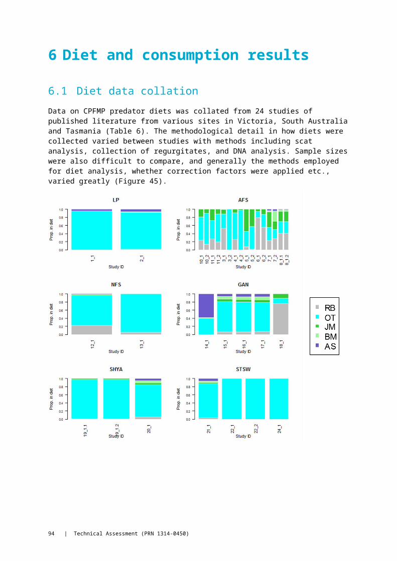
Table 13 A list of data collection and monitoring indices for informing spatial management options (see text for explanation of ranking categories). The table does not contain an exhaustive list of options but indicates the types of variables which would need to be considered in a design study for monitoring CPFMP in relation to fishery operations.
MONITORING DATA SEABIRDS SEALS RANKING RATIONALE RANGE
Diet during CPF period RegurgitatesIsotopesDNA
Scats/regurgitatesStable isotopesDNA
Basic Characterise annual and spatial variability in diet proportion relative to SPF
abundance indices.
Where gaps exists and at key monitoring sites
Offspring mass at end of provisioning period or for a standardized time within the provisioning period
Basic Determines relationship between weaning/fledging weights and prey
availability via SPF abundance indices
Key monitoring sites
Number of individuals breeding
Breeders to moulters ratio (penguins)
Pup counts Basic Monitor population breeding success vs effort
Key monitoring sites
Burrow/nest occupancy vs breeding (shearwaters, gannets)
Basic Key monitoring sites
Collection of telemetry data in regions where none exist
Desirable Fill in gaps in the coverage of at-sea distribution data. This should be done
tactically as required in response to likely areas of fishery operation (if known) or in
areas of key ecological interest (e.g. upwelling zones). Note the use of TDRs in conjunction with tracking instruments is
desirable for comprehensive characterisation of spatial distribution of
foraging behaviour/effort
Where gaps exist (e.g. Tasmanian colonies for most CPF species considered)
Attendance patterns of provisioning adults at colonies
Desirable Index of foraging effort in relation to availability (e.g. using PIT tags / VHF
transmitters to monitor presence absence at colonies)
Key monitoring sites or in zones of fishery operation
Pup growth rates Desirable Integrated index of prey availability / foraging success
Key monitoring sites
Adult mass at commencement provisioning period
Optimal Determine the foraging success / prey availability in intervening non-breeding period. Examine seasonal effects and
vulnerability
Key monitoring sites
Age specific annual survival and recruitment
Optimal Examine whether there are regional differences in vital rates which may be
related to spatial variation in prey availability.
Key monitoring sites
Chronology/phenology of breeding
Optimal Examine whether breeding was delayed, relative to SPF abundance indices and
climate variability.
Key monitoring sites
In order to discern potential negative effects of fisheries activities from the effects of natural environmental variability, monitoring of basic indices (Table 13) should be conducted annually. This is because breeding success in any given year may be due to environmental variation (Peck et al. 2004, Smithers et al. 2004, McIntosh et al. 2013) or unforeseen events such as disease outbreaks (Bunce and Norman 2000a, Dann et al. 2000) which might suppress breeding success and it is often advisable to make management decisions based on trends assessed over a period of years rather than data from any particular year.
The choice of colonies for monitoring should be considered as part of a detailed design study. Obviously large colonies are more important to persistence of the overall population and also account for a large proportion of the impact on the SPF target species. However, changes at larger colonies may need to be more pronounced before they can be detected. Therefore, some consideration of the characteristics of
Technical Assessment (PRN 1314-0450) | 95

colonies best suited for monitoring is required. We consider that monitoring colonies ought to be spatially distributed in a way that can account for the influence of differences in prevailing oceanography. Variability in regional current and upwelling systems such as the EAC (Young et al. 1993, Jordan et al. 1995, McLeod et al. 2012), the Flinders Current, the Bonnie Upwelling region are expected to have large ecosystem effects on prey density.
While desirable, annual monitoring of spatial habitat use by CPFMP from telemetry studies may not be feasible due to the number of colonies, number of species involved and the geographic extent they cover across the SPF (hence the listing of desirable in Table 13). However, understanding of the potential habitat use across different environmental conditions is required. Hence, where telemetry studies have not already conducted, information on spatial habitat use should be obtained for the monitoring sites over a number of years to cover natural environmental variability. This is necessary to fill in the regional gaps in understanding spatial distribution and be used to characterize differences in foraging range, general foraging habits and characterize the degree of variability in at-sea distribution. Chiefly this would consist of further tagging effort being made in Tasmania, Western Australia and New South Wales (again, noting that work is underway at Montague Island, NSW).
Given the issues noted with spatial modelling in section 5, we also recommend further assessment and development of at-sea distribution models. The models we considered were limited and could be further refined. This might include the use of mixture models, as per Goldsworthy et al. (2013), investigation of cross validation methods (Matthiopoulos 2003) or more complex models explicitly incorporating the structure of foraging trips (Patterson 2010 ).
11.2 Management Strategy Evaluation
This report has shown that the design of effective spatial management measures will involve a mix of quantitative (predatory spatial distribution, population sizes, diet data) and semi-quantitative uncertainties (prey density and dynamics, functional responses). Additionally, there is a stated intention to implement harvest control rules on the fishery to account for potential prey depletion effects on the central place foragers (AFMA 2013). Taken together, this suggests the use of management strategy evaluation (MSE) as an appropriate tool for formally assessing the relative efficacy of different spatial management options in relation to minimising the impact on CPFMP populations the SPF. MSE is essentially a simulation method for examining how management actions are likely to perform given uncertainty about the true state of a system (Rademeyer et al. 2007). In a single species fisheries setting, where the MSE methodology has been most widely applied, setting up a minimal MSE requires three components (depicted graphically in Figure 49).
(i) a set of observations (e.g. a survey abundance index) used in the assessment /management process
(ii) either an empirical or model-based “assessment” that estimates the relevant parameters (e.g. log-scale trend in the abundance index) from these data, and
(iii) a control rule that takes these parameter estimates and turns them into the proposed management outcome (e.g. an increase/decrease in the TAC from the previous year; a change in the area of operation of the fishery).
Additionally, the MSE also requires a realistic simulation model known as the operating model. This aims to realistically model the relevant aspects of the ecological system under consideration and the influences of harvesting upon it. Essentially this is a hypothesis about the relevant components of the system and how they interact. It could be complex (such as the full ecosystem model developed by Fulton et al. (2011), or something more streamlined such as a multispecies population dynamics model (Butterworth and Plaganyi 2004).
96 | Technical Assessment (PRN 1314-0450)

Operating Model
Synthetic data series
Simulated harvesting
Control rule/Management procedure
Figure 49 The basic components of a management strategy evaluation. The operating model is a detailed simulation model which may include several sub-models which simulate population dynamics (of relevant system components – e.g. predators and prey), fishery dynamics via fleet dynamics models and the effects of harvesting and management constraints on these. The data model simulates a survey of relevant parts of the system (e.g. catch data collection, monitoring of predator populations) and importantly, the errors in inherent in these.
Given the primary focus of the current work is the potential for effects on central place foragers that prey on the SPF target species, and not necessarily the wider ecosystem, the use of Ecosystem Models of Intermediate Complexity or MICE (Plaganyi et al., 2012) would seem to be the most appropriate framework to place any future MSE initiative within. This form of model is constructed to only include the principle processes of interest (hence “minimally” realistic), and to formally estimate parameters from data using statistical estimation methods, where feasible. In this sense, they are more akin to modern, statistical population models and allow for uncertainty across the sub-system under consideration to robustly characterised, in a formal statistical framework. A spatially resolved model of this nature would seem an appropriate if considering an MSE framework to test potential management measures as it would be provide for the direct integration of the methods and results from this initial work and be constructed with the appropriate spatial and temporal scales to specifically address the objectives of any proposed spatial management measures and the interaction with SPF target species population. In terms of factors to consider in the design of spatial management measures, spatio-temporal allocations of catch and/or effort are obvious choices (as outlined in section 10).
In the context of the SPF, and consideration of spatial management options which aim to lower the risk of fisheries operations leading to local depletion, we need to outline some detail on each of these components so that they are relevant to the CPFMP populations under consideration.
(1) The operating model: This would need to be made up of the following sub-components:a. Models of the SPF target species population dynamics. A variety of model complexities
could be considered but, at the least, these should simulate strong and weak years of prey abundance in a spatial sense. This could be simulated statistically for example, as a random process with a trend and variance potentially based on survey indices (Ward et al. 2011a), or using population models. This would need to be spatially resolved, at least at the level of a relevant fisheries management unit.
b. Spatially resolved model of the population dynamics of the CPFMP. This could be parameterised using available life tables etc. But crucially CPFMP population dynamics would need to be linked to prey abundance. For example production of young and their survival could be simulated as a function of prey abundance obtained from the prey dynamics model. The spatial aspects of the CPFMP model could be either quite detailed
Technical Assessment (PRN 1314-0450) | 97

such as high resolution simulation of foraging trips, or much simpler, such as a model of the number of predators within a spatial block, their bulk movement rates between blocks and their likely foraging success and impacts on the prey population within each spatial block. The simpler version of this model is more likely to be tractable and we guess would provide the required resolution without the added complexity of simulating individual movements and foraging success. However, certain spatial management options may require determining the likely time spent within a closed area which might conceivably be smaller than the spatial units of the operating model (see point d below).
c. Fleet dynamics model: The operating model would also need to include a simulated fishery operating according to a set of spatial management measures, other regulatory constraints and plausible socio-economic incentives. At its simplest level, the fishers would be assumed to operate like another predator with an associated functional response which dictated their likely effort and catch distributions, given the simulated target species abundance and information flow among vessels/operators (Little et al. 2004). Optionally, it could also include economic constraints such as fuel costs, market fluctuations etc. depending on the particular level of interest. These further complexities may be unnecessary for an assessment of spatial management options or may be approximated by the use of less direct variables, such as distance from home-port for fuel costs. The important point is to encapsulate the likely behaviour of the fleet to the combination of spatial management measures, distribution and abundance of prey species and other constraints on them meeting their general fishing objectives (referred to as “maximising their utility”). This will be central to evaluating the trade-offs between an acceptable economic return/impacts from a fishery perspective versus the potential impacts on the CPFMP populations. It is at the level of the fisheries dynamics model that the spatial management options (options 1-4 in section 10), and the details of their potential implementation, would be implemented in an MSE modelling exercise. For example, simulated vessels might be required to spatially distribute their effort or operate according to a move-on rule. Additionally, if spatial closures around colonies were considered, the biomass of prey within these areas would be unavailable to the fishery, while in that area. The MSE approach would allow different assumptions about fleet dynamics, rates of mixing and movement of prey populations and foraging and breeding and seasonal movements of CPFMP on the performance of different spatial management options to be explicitly explored. This is very helpful in refining the design of alternative strategies and identifying assumptions that different strategies are particularly sensitive to. In turn this provides an objective and directed basis for prioritising research and monitoring activities.
(2) The “observation model” would include both fisheries abundance indices, such as from catch data, egg-production or other surveys of prey biomass (Ward et al. 2011a, Ward et al. 2011b, Ward et al. 2012), and also time series of predator productivity and abundance. The monitoring work in other overseas settings (e.g. Frederiksen et al. (2004) and CCAMLR (2014 )) has recommended that indices of pup and chick production are likely to be the most appropriate for detecting effects in the short term (See monitoring recommendations below). Abundance of adults could be inferred from these using appropriate multipliers or from adjunct surveys of adults where appropriate. Importantly, the observation model would need to consider the likely precision and possible biases in catch and effort data from the fishery and from predator productivity and abundance surveys.
98 | Technical Assessment (PRN 1314-0450)

These would most straightforwardly be parameterized in terms of addition of simulated “noise” or errors around the “true” simulated values from the operating model (e.g. Conn et al. (2014)).
(3) Control rules would need to be devised which set out, ahead of time and generally in accordance with consultation with relevant stakeholders, the management response which will be enacted should the observations (detailed in 2 above) indicate that the various components of the system (here the target species and CPFMP) have changed. For example, if a large drop in CPUE were detected in the fishery data for they prey species, this might trigger a reduction of the TAC by an agreed amount in the relevant spatial regions. Similarly, a large drop in breeding success by a CPFMP may indicate that depletion of prey resources by the fishery could be responsible and reductions in TACs may result. At this point an obvious issue arises in detecting when the fishery is a likely cause versus background variability in prey resources. A further crucial aspect to recognise is that the control rule would be linked to the status of the predator populations.
An MSE as proposed here would have two significant outcomes:(1) An initial or tactical set of recommendations of the efficacy of spatial management options given
the current state of knowledge in the fishery and an understanding of which is likely to be most robust to uncertainty.
(2) An evaluation of a robust monitoring program, how this would feed into a harvest strategy and setting of catch limits and other management actions.
It is important to emphasise that while an MSE would be the quicker option to providing an indication of the efficacy of spatial management options, it would nonetheless entail a substantial amount of work. Were this route to be adopted, a necessary next step would therefore be a workshop or similar forum which could bring together experts on both the fishery, the predators, MSE practitioners and relevant stakeholders and management representatives to outline a set of spatial and other management scenarios to explore, consider details of survey logistics, likely colonies to monitor and develop a set of operating model scenarios which bound the likely uncertainty about the interactions between predators, prey, fisheries and environmental variability.
Predation forms a key part of the overall natural mortality rate of prey species such as those in the SPF. So attempting to manage spatiotemporal catch levels so as not to exceed sustainable fishing mortality levels could have a dual impact:
1. linkage with single-species sustainable management of the SPF as per Harvest Strategy; and 2. ensuring that the fishery does not remove too much prey abundance at the finer spatial scales that
might impinge on the predators feeding requirements.
Importantly, the purpose of the MSE, is not to predict the specific outcomes of using such a spatial management rule, as this is highly unlikely to be fruitful given the uncertain and dynamic nature of these systems; rather it is to compare the performance against alternatives, including the status quo, under the same conditions (i.e. the minimally realistic model) and, importantly, including the major sources of uncertainty in the system of interest. This allows the performance, behaviour, sensitivity and potential cost-effectiveness of different management options to be considered before proceeding to selecting and implementing a preferred alternative in reality.
Technical Assessment (PRN 1314-0450) | 99

12 Discussion
This report has collated and summarized colony location, size and population status for 6 species of central place foraging marine predators that are found in waters which constitute the Commonwealth Small Pelagic Fishery.
Our report indicates that there are large uncertainties in the abundance and distribution of colonies with many estimates being out of date or without estimates of uncertainty. The number of well-studied and monitored sites is small with very few having detailed population structure information.
The study also compiled estimates of the predator’s diet from the literature and found a high degree of variability between studies. Obtaining estimates of the diet of free ranging marine predators is challenging but standardization of methods throughout the SPF would aid in developing a more robust picture of CPFMP in the SPF.
The quality and quantity of tracking data varies greatly with only a few areas in Bass Strait having large, high quality data sets. Additionally very little tracking data exists from Tasmania and NSW. The authors are aware of recent tracking efforts at Montague Island (R. Harcourt, Macquarie University, Pers. Comm.) which should yield further important data in the future.
Behaviour switching models (hidden Markov models) showed substantial variability between species on the intensity of foraging given distance-from-colony. However, all seabird species in the tracking data examined here foraged within 100km of their colony. For the pinnipeds these distances were larger. However, the New Zealand fur seal tracking dataset is too small for reliable inference and further collection of New Zealand fur seal movement data from within Bass Strait and Tasmania is necessary to quantify their foraging range.
The examples of at-sea distribution models shown here indicate that this area is challenging. Tracking data reflects complex processes of foraging, with animals alternating between active foraging, colony residence, resting phases and searching or transiting movements. Capturing this complexity with simple models is challenging. As a result the models we examined here typically fit the case study data poorly and were liable to overstate their statistical accuracy due to assumptions of independence. The fits from the obtained here may well be particular to the data sets we examined. Hence, we cannot draw conclusions on the performance of either proximity models or GAMS in other settings, where they may well be fit for purpose, despite the issues we outline. Irrespective, further consideration and refinement spatial models for at-sea distribution within the SPF is necessary to assess the degree of specificity (e.g. models for colonies, age classes, by sex). Moreover, any future modelling of spatial distribution needs to be carefully integrated with the management and assessment framework to ensure that models are fit for purpose, robust and only as complex as is actually necessary for evaluating spatial management options.
The at-sea distribution modelling approaches considered here come with strengths and some disadvantages. Modelling and predicting animal movements in novel environment (where spatial data are lacking) based on individual animal tracking data are one of the key problems in ecology (Patterson et al. 2008). The methods for at-sea distribution modelling investigated in this report are extremely simple considering the complexity of the processes we are seeking to model. Reducing model complexity is always desirable if the models can capture the salient aspects of the data, but it is necessary to determine if the key properties of the data are well replicated by the models. In management settings it is generally advantageous if the models can be kept simple and interpretable, do not rely on a large number of predictor variables. In this sense, the two predictor variables of distance from colony and bathymetry seem well suited to the problem. However, A priori, both the at-sea distribution model types considered here fail to account for important features of movement data and the dynamics of central place foragers. Neither type of model accounts for the ubiquitous auto-correlation inherent in individual tracking data. This tends to have the effect that data are assumed to contain higher levels of information than they really do—an aspect which may lead to spuriously precise estimates of parameters and, therefore, spuriously precise estimates of spatial usage and we expect, also spatial consumption. The degree to which this is a problem is
100 | Technical Assessment (PRN 1314-0450)
difficult to gauge without building spatial models which can account for non-independence in CPFMP spatial data. Another option for testing these models and their ability to predict the distribution in novel areas would be a cross validation exercise, either within data sets from different colonies.
Further, it would be useful to conduct rigorous cross-validation exercises within the data sets which are available. This would involve leaving out some of the data from the models and using these as test data sets to examine the ability of the at-sea distribution models to predict the withheld data. Such an exercise is beyond the scope of the current project but is highly achievable given sufficient time.
Proximity models using the parametric forms considered here (i.e. the Gamma and Normal PDFs) are attractive because they require few parameters and are straightforward to fit. They also lead to directly interpretable predictions of foraging zones and the Gamma distribution is guaranteed to predict decreasing spatial usage at greater distances from a colony. However, proximity models also assume that foraging-distance and bathymetry are independent variables. This is unlikely to be the case given that colony location and bathymetry are correlated because colonies are by definition in close proximity to shallow water. Additionally, the form of the Gamma and Gaussian PDFs may not adequately model the distribution of long-distance foraging in species that cover large distances to forage. By virtue of their shape, where the probability mass is skewed towards zero (if the distribution has long tails), there is potential for these models to under-represent the amount of time spent further from colonies. If this is the case for a given data set, this bias could conceivably lead to a less precautionary assessment of at-sea distribution.
Generalized additive models were selected in this context as a flexible modelling framework which can cope with over-dispersed data. However, as mentioned, the GAMs deployed here do not account for the autocorrelation in the data. Additionally, the smoothing splines employed in GAMS often make highly implausible predictions outside the range of fitted data. This means one has to be careful about transporting GAMs to new locations and be careful to restricting the spatial extent of their predictions to the spatial regions for which they have been developed.
While construction of state-of-the-art spatial models was beyond the constraints of this project, it is possible to list the properties of such models as a guide for any future research. A more in-depth and considered analysis would construct spatial distribution models that would directly account for the trip-based behavior of CPF species. This would need to account for animals making a variable length outward transit leg, undertaking active foraging and searching, and finally returning to the colony (Patterson 2010 ). While there are examples of models of this sort in the literature (Matthiopoulos 2003, Wakefield et al. 2009), constructing them is not a straightforward exercise and generally remains an open research question which is yet to settle on accepted modelling techniques. A recent paper by (Raymond et al. 2014) has developed approaches to this, in what amounts to a more complex and comprehensive instance of the HMM and GAM modelling used here. With further time and representative data, it is likely that models of at-sea distribution which are credible for decision making and management purposes could be constructed.
The study noted that the key variability for CPFMP is likely to be during phases of raising young. The vulnerability analysis highlighted the summer breeding phases as most vulnerable. However, the study is unable to account for the potential for non-breeding mature animals to be affected outside this period. It is feasible that depletion of prey resources over the non-breeding phases might lead to decreased investment in breeding phase. This cannot be determined from current data, although note that we recommend monitoring of survival rates which could be done with mark-recapture models. Annual estimates of survival may provide some useful information on this. Nonetheless, tracking of non-breeding mature individuals which remain in the SPF would be an important step in addressing this. Additionally, improved energetic budgets could allow for characterization of reduced maternal investment in pups, for example. This has been examined in relation to climate other species and contexts and is now being incorporated into models e.g. (New et al. 2011, Schick et al. 2013) but these are in the early phase of development.
Understanding the details of the biological processes at work here such as foraging dynamics, investment in young, prey availability, environmental variability is an extremely large and complex task. As a result, any future research which is to inform management ought to be evaluated prior to large scale field collection to gauge its value in a management context. Examples of this exist, such as (Butterworth 2007), where a power analysis of particular monitoring programs was conducted to estimate the necessary length of a
Technical Assessment (PRN 1314-0450) | 101
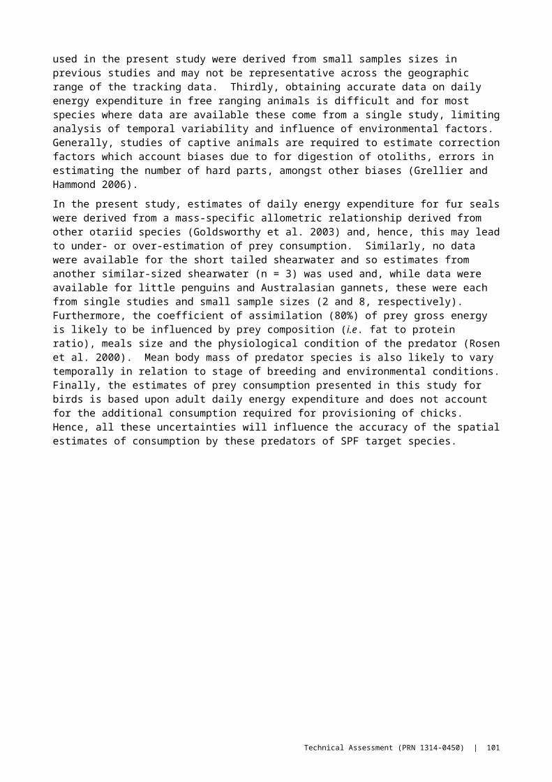
sampling program required to detect a given effect size on breeding success parameters in South African penguin populations. These sorts of analyses could be conducted within an integrated MSE.
The estimates of consumption developed in this study were necessarily simple and intended to demonstrate the form of approach that might be used in a more comprehensive exercise. Although the estimates given here are limited, they do indicate that the total consumption of the CPFMP indicated by these examples is likely to be very large relative to likely TACs or recommended biological catch limits for the SPF.
102 | Technical Assessment (PRN 1314-0450)

13 Summary of findings and recommendations
This section outlines the findings of the report against the deliverables requested in the project services agreement.
1. The current report has assessed the role for spatial management strategies in mitigating the potential direct and indirect effects of fishing by large mid-water trawl vessels in the SPF on central-place foraging species.
We found that spatial management has potential to play a significant role in minimising the risks of fishing by large mid-water trawl vessels in the SPF on CPFMP. However, we found that in many places the necessary information and data to support the design of management strategies is lacking or out of date. We have recommended monitoring strategies, further collection of dietary data, revised colony abundance estimates and representative tracking data in regions where data are lacking. We also recommend that a Management Strategy Evaluation exercise is carried out to assess particular spatial management options. If spatial management measures are to be introduced in the SPF, it is crucial that concurrent integrated monitoring is conducted so that robust indices of predator breeding performance and population growth are available for incorporation into SPF decision rules and management procedures. We have prioritised classes of population indices which would be needed for establishing time series of data which are likely to be appropriate in this regard.
2. The report has, subject to available information and data, used existing available data on at-sea distributions, diet and population size of central-place foraging species within the SPF to construct models of at-sea distribution.
(i) The report constructed and evaluated models of CPFMP at-sea distributions, density and likely prey consumption of SPF targeted species.
We constructed at-sea distribution models based on case study data for Bass Strait. We calculated aggregate prey consumption with uncertainty given available abundance estimates for the six CPFMP species considered. We considered two scenarios of prey stock depletion and three different functional response scenarios. In order to be precautionary, we used diet studies which reported highest diet proportion of SPF target species.
This found that estimates of consumption for some species (notably pinnipeds) was likely to be significantly larger than historic TACs for the SPF even when accounting for reported uncertainties on abundance estimates and incorporating uncertainty on proportion of SPF target species in the predator’s diet.
We examined the potential for predicting the density of predators, but given the gaps in the available data telemetry data, we provided a demonstration of spatial consumption estimation (with associated uncertainty) at a scale which might be employed in fisheries management. We found that the assumptions of the spatial models we investigated are likely to result in under-representation of the degree of uncertainty in estimates of the spatial distribution of predators, and hence similarly affect estimates of their spatial density. This aspect requires further work and should be re-visited in detail to assess whether existing models can be improved in this regard.
(ii) The report has identified, where possible, for central-place foraging species, the likely regions and times-of-year in which they may be most vulnerable to potential ecological effects of fishing, such as depletion of prey, and to interactions with fishing operations.
We examined the seasonal cycles of breeding for CPFMP species and their foraging strategies. It is likely that CPFMP species are likely to be most at risk from localised depletion effects during peak breeding
Technical Assessment (PRN 1314-0450) | 103

periods over the summer months. However, there are very large uncertainties regarding foraging and distribution of CPFMP during the non-breeding periods and it is possible that reduced prey availability could reduce a predator’s ability to restore energy reserves for subsequent breeding. We cannot make definitive statements in this regard due to the lack of available data. Additionally, the poor coverage of tracking studies throughout the entire SPF (excepting South Australia and parts of Bass Strait) means that there are currently insufficient data for deciding which specific small scale regions are most likely to be vulnerable throughout SPF waters adjacent to the majority of the Western Australian, Tasmanian and New South Wales coast.
The report was unable to make definitive statements about likely direct interactions with the fishery. To do so would require detailed and specific information on likely fishing locations, intensities, gear type or access to fine scale catch and effort data. We consider that our spatial analysis results and the listing of gaps in the spatial and abundance data should provide useful background for further work on direct interaction. We note that Tuck et al. (2013) stated that there were relatively few interactions with CPFMP species in the SPF which led to direct mortality. However, Tuck et al. (2013) also noted caveats regarding observer coverage and the general reduction in effort in recent years of SPF operations relative to historical levels.
3. This report has conducted an assessment of the best methodological approaches to identify potential locations, size and timing of spatial management to mitigate the potential ecological effects of fishing on, and interactions with, central-place foraging species by large mid-water trawl vessels in the SPF. We have included in this report case-study references to significant global examples where spatial management has been used to mitigate ecological and bycatch impacts on central-place foraging species.
We have outlined a research program which would specifically incorporate the best available methodology for identifying potential locations for spatial management. Our recommended approach follows along the lines of the CCAMLR precautionary approach to Ecosystem based fisheries management. We considered four main categories of spatial management measures
(i) Setting a TAC that accounts for the necessary requirements of predators;
(ii) allocation of TACs spatially to ensure that catches are not concentrated in any one spatial zone;
(iii) spatial closures around key breeding sites during periods of peak breeding activity; and
(iv) the use of a move-on rule which might specify a proportion of an operator’s quota which could be extracted within any one spatial zone over a suitably defined period of time.
The latter would be expressly aimed at maintaining prey aggregations and prey fill-in rates at sufficient levels to minimize local prey-depletion risks. Establishing the precise details of these proposed measures and the particular permutations thereof, requires extensive consultation with a range of stakeholders and experts, the formulation of candidate decision rules, and testing through an appropriate MSE as described herein.
4. We have identified further research that may be required in order to identify key ecologically sensitive species, areas and times where spatial management strategies may be appropriate to mitigate the potential ecological effects of fishing on, and interactions with, central-place foraging species in the SPF.
We note that our case study CPFMP species were restricted to those for which we had ready access to relevant data. Therefore our report does not encompass the full range of predator species which could be potentially impacted by operation of large mid-water trawls.
Our recommendations for further research are summarized as follows:
104 | Technical Assessment (PRN 1314-0450)

1. To address the noted gaps in telemetry data at a regional scale, to obtain further diet data, preferably over multiple seasons to assess variability in the diet of SPF species.
2. To establish an integrated monitoring program at a spatially representative set of reference colonies for each species. We consider that many aspects of predator breeding especially need to be assessed annually in an attempt to disentangle environmental variability from potential fishery impacts. Additionally, annual surveys would allow management decisions to be made on the basis of trends in predator productivity rather than solely on data for any given year.
3. To conduct an MSE which would most likely employ minimally realistic models/models of intermediate complexity to evaluate spatial management options in a quantitative manner and link with the design aspects, as per point 2 above.
Technical Assessment (PRN 1314-0450) | 105
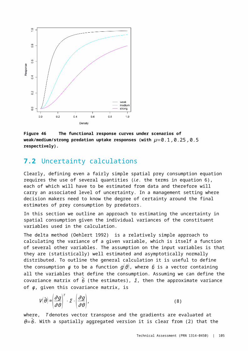
14 Bibliography
AFMA. 2010. Australian Sea Lion Management Strategy, Southern and Eastern Scalefish and Shark Fishery (SESSF) AFMA, Canberra.
AFMA. 2013. Small Pelagic Fishery Harvest Strategy.Angel, L. P., and J. P. Y. Arnould. in press. Sexual size dimorphism in the Australasian Gannet. Emu.Argos, C. 2008. Argos Users Manual.Arim, M., and D. E. Naya. 2003. Pinniped diets inferred from scats: analysis of biases in prey occurrence.
Canadian Journal of Zoology-Revue Canadienne De Zoologie 81:67-73.Arnould, J., and R. Warneke. 2002. Growth and condition in Australian fur seals (Arctocephalus pusillus
doriferus)(Carnivora: Pinnipedia). Australian Journal of Zoology 50:53-66.Arnould, J. P., and M. A. Hindell. 2002. Milk consumption, body composition and pre weaning growth rates ‐
of Australian fur seal (Arctocephalus pusillus doriferus) pups. Journal of Zoology 256:351-359.Arnould, J. P. Y., and M. A. Hindell. 2001. Dive behaviour, foraging locations, and maternal-attendance
patterns of Australian fur seals (Arctocephalus pusillus doriferus). Canadian Journal of Zoology-Revue Canadienne De Zoologie 79:35-48.
Arnould, J. P. Y., and R. Kirkwood. 2008. Habitat selection by female Australian fur seals (Arctocephalus pusillus doriferus). Aquatic Conservation-Marine and Freshwater Ecosystems 17:S53-S67.
Atkinson, S., D. P. DeMaster, and D. G. Calkins. 2008. Anthropogenic causes of the western Steller sea lion Eumetopias jubatus population decline and their threat to recovery. Mammal Review 38:1-18.
Auster, P. J., K. Gjerde, E. Heupel, L. Watling, A. Grehan, and A. D. Rogers. 2011. Definition and detection of vulnerable marine ecosystems on the high seas: problems with the “move-on” rule. ICES Journal of Marine Science: Journal du Conseil 68:254-264.
Basson, M. 1999. The importance of environmental factors in the design of management procedures. ICES Journal of Marine Science: Journal du Conseil 56:933-942.
Baylis, A. M., B. Page, J. McKenzie, and S. D. Goldsworthy. 2012. Individual foraging site fidelity in lactating New Zealand fur seals: Continental shelf vs. oceanic habitats. Marine mammal science 28:276-294.
Baylis, A. M. M., D. J. Hamer, and P. D. Nichols. 2009. Assessing the use of milk fatty acids to infer the diet of the Australian sea lion (Neophoca cinerea). Wildlife Research 36:169-176.
Baylis, A. M. M., B. Page, and S. D. Goldsworthy. 2008. Effect of seasonal changes in upwelling activity on the foraging locations of a wide-ranging central-place forager, the New Zealand fur seal. Canadian Journal of Zoology 86:774-789.
Beaugrand, G. 2004. The North Sea regime shift: evidence, causes, mechanisms and consequences. Progress in Oceanography 60:245-262.
Begg, G. A., K. D. Friedland, and J. B. Pearce. 1999. Stock identification and its role in stock assessment and fisheries management: an overview. Fisheries Research 43:1-8.
Bool, N., B. Page, and S. D. Goldsworthy. 2007. What is causing the decline of little penguins (Eudyptula minor) on Granite Island, South Australia. SARDI Research Report Series.
Boyd, C., A. E. Punt, H. Weimerskirch, and S. Bertrand. 2014. Movement models provide insights into variation in the foraging effort of central place foragers. Ecological Modelling 286:13-25.
Boyd, I., and A. Murray. 2001. Monitoring a marine ecosystem using responses of upper trophic level predators. Journal of Animal Ecology 70:747-760.
Brothers, N., R. Gales, and D. Pemberton. 1993. Prey harvest of the Australasian gannet (Sula serrator) in Tasmania. Wildlife Research 20:777-783.
Brothers, N., and D. Pemberton. 1990. Status of Australian and New-Zealand Fur Seals at Maatsuyker Island, Southwestern Tasmania. Wildlife Research 17:563-569.
Bunce, A. 2001a. Prey consumption of Australasian gannets (Morus serrator) breeding in Port Phillip Bay, southeast Australia, and potential overlap with commercial fisheries. ICES Journal of Marine Science: Journal du Conseil 58:904-915.
Bunce, A. 2001b. Prey consumption of Australasian gannets (Morus serrator) breeding in Port Phillip Bay, southeast Australia, and potential overlap with commercial fisheries. Ices Journal of Marine Science 58:904-915.
106 | Technical Assessment (PRN 1314-0450)

Bunce, A. 2004. Do dietary changes of Australasian gannets (Morus serrator) reflect variability in pelagic fish stocks? Wildlife Research 31:383-387.
Bunce, A., and F. Norman. 2000a. Changes in the diet of the Australasian gannet (Morus serrator) in response to the 1998 mortality of pilchards (Sardinops sagax). Marine and Freshwater Research 51:349-353.
Bunce, A., F. Norman, N. Brothers, and R. Gales. 2002. Long-term trends in the Australasian gannet (Morus serrator) population in Australia: the effect of climate change and commercial fisheries. Marine Biology 141:263-269.
Bunce, A., and F. I. Norman. 2000b. Changes in the diet of the Australasian gannet (Morus serrator) in response to the 1998 mortality of pilchards (Sardinops sagax). Marine and Freshwater Research 51:349-353.
Burek, K. A., F. M. Gulland, G. Sheffield, K. B. Beckmen, E. Keyes, T. R. Spraker, A. Smith, E. Douglas, J. F. Skilling, J. L. Evermann, J. T. Stott, J. Saliki, and A. W. Trites. 2005. Infectious disease and the decline of Steller sea lions (Eumetopias jubatus) in Alaska, USA: insights from serologic data. Journal of Wildlife Diseases 41:512-524.
Butterworth, A. B. a. D. S. 2007. An Initial Analysis of the Power of Monitoring certain Indices to Determine the Effect of Fishing on Penguin Reproductive Success from an Experiment where Pelagic Fishing is Prohibited in the Neighbourhood of Robben Island, but Continues around Dassen Island
Butterworth, D., and E. Plaganyi. 2004. A brief introduction to some approaches to multispecies/ecosystem modelling in the context of their possible application in the management of South African fisheries. African Journal of Marine Science 26:53-61.
Camphuysen, C., B. Scott, and S. Wanless. 2006. Distribution and foraging interactions of seabirds and marine mammals in the North Sea: multispecies foraging assemblages and habitat-specific feeding strategies.
Capuska, G. E. M., R. L. Vaughn, B. Wursig, G. Katzir, and D. Raubenheimer. 2011. Dive strategies and foraging effort in the Australasian gannet Morus serrator revealed by underwater videography. Marine Ecology Progress Series 442:255-261.
CCAMLR. 2008. Report of the twenty-seventh meeting of the scientifc committee, SC-CAMLR XXVII. Hobart, Australia.
CCAMLR. 2011. Report of the thirtieth meeting of the scientific committee, SC-CAMLR-XXX. Hobart, Australia.
CCAMLR. 2012. Schedule of Conservation Measures in Forces, 2011/12. Hobart, Australia.CCAMLR. 2014 CCAMLR Ecosystem Monitoring Programme Standard Methods. CCAMLR, Hobart, Tasmania.Chiaradia, A., A. Costalunga, and K. Kerry. 2003. The diet of Little Penguins (Eudyptula minor) at Phillip
Island, Victoria, in the absence of a major prey–Pilchard (Sardinops sagax). Emu 103:43-48.Chiaradia, A., M. G. Forero, K. A. Hobson, and J. M. Cullen. 2010. Changes in diet and trophic position of a
top predator 10 years after a mass mortality of a key prey. ICES Journal of Marine Science: Journal du Conseil 67:1710-1720.
Chiaradia, A., M. G. Forero, K. A. Hobson, S. E. Swearer, F. Hume, L. Renwick, and P. Dann. 2012. Diet segregation between two colonies of little penguins Eudyptula minor in southeast Australia. Austral Ecology 37:610-619.
Chiaradia, A., Y. Ropert-Coudert, A. Kato, T. Mattern, and J. Yorke. 2007. Diving behaviour of Little Penguins from four colonies across their whole distribution range: bathymetry affecting diving effort and fledging success. Marine Biology 151:1535-1542.
Chilvers, B. L. 2008. New Zealand sea lions Phocarctos hookeri and squid trawl fisheries: bycatch problems and management options. Endangered Species Research 5:1-12.
Coetzee, J. C., C. D. van der Lingen, L. Hutchings, and T. P. Fairweather. 2008. Has the fishery contributed to a major shift in the distribution of South African sardine? ICES Journal of Marine Science: Journal du Conseil 65:1676-1688.
Conn, P. B., D. S. Johnson, L. W. Fritz, and B. S. Fadely. 2014. Examining the utility of fishery and survey data to detect prey removal effects on Steller sea lions (Eumetopias jubatus). Canadian Journal of Fisheries and Aquatic Sciences 71:1229-1242.
Technical Assessment (PRN 1314-0450) | 107

Connan Maëlle, M. P., Hobson Keith, Weimerskirch Henri, Cherel Yves 2010. Food and feeding ecology of the Tasmanian short-tailed shearwater (Puffinus tenuirostris, Temminck): insights from three complementary methods. Journal of Oceanography, Research and Data 3:13.
Constable, A., and S. Nicol. 2002. Defining smaller-scale management units to further develop the ecosystem approach in managing large-scale pelagic krill fisheries in Antarctica. CCAMLR Science 9:117-131.
Constable, A. J. 2011. Lessons from CCAMLR on the implementation of the ecosystem approach to managing fisheries. Fish and Fisheries 12:138-151.
Costa, D. P., P. Dann, and W. Disher. 1986. Energy-Requirements of Free Ranging Little Penguin, Eudyptula-Minor. Comparative Biochemistry and Physiology a-Physiology 85:135-138.
Costa, D. P., and N. J. Gales. 2003. Energetics of a benthic diver: Seasonal foraging ecology of the Australian sea lion, Neophoca cinerea. Ecological Monographs 73:27-43.
Costa, D. P., P. W. Robinson, J. P. Arnould, A.-L. Harrison, S. E. Simmons, J. L. Hassrick, A. J. Hoskins, S. P. Kirkman, H. Oosthuizen, and S. Villegas-Amtmann. 2010. Accuracy of ARGOS locations of pinnipeds at-sea estimated using Fastloc GPS. PloS one 5:e8677.
Crawford, R. J. M., P. J. Barham, L. G. Underhill, L. J. Shannon, J. C. Coetzee, B. M. Dyer, T. M. Leshoro, and L. Upfold. 2006a. The influence of food availability on breeding success of African penguins Spheniscus demersus at Robben Island, South Africa. Biological Conservation 132:119-125.
Crawford, R. J. M., E. Goya, J. P. Roux, and C. B. Zavalaga. 2006b. Comparison of assemblages and some life-history traits of seabirds in the Humboldt and Benguela systems. African Journal of Marine Science 28:553-560.
Crawley, M., and G. Wilson. 1976. The natural history and behaviour of the New Zealand fur seal (Arctocephalus forsteri). Biological society, Victoria University of Wellington.
Cullen, J. M., L. E. Chambers, P. C. Coutin, and P. Dann. 2009. Predicting onset and success of breeding in little penguins Eudyptula minor from ocean temperatures. Marine Ecology Progress Series 378:269-278.
Cunningham, C. L., and D. S. Butterworth. 2006. Issues surrounding the development of a revised OMP for the SA Pelagic Fishery for Sardine and Anchovy. SWG/MAY2006/PEL/09.
Cury, P., A. Bakun, R. J. Crawford, A. Jarre, R. A. Quiñones, L. J. Shannon, and H. M. Verheye. 2000. Small pelagics in upwelling systems: patterns of interaction and structural changes in “wasp-waist” ecosystems. ICES Journal of Marine Science: Journal du Conseil 57:603-618.
Cury, P. M., I. L. Boyd, S. Bonhommeau, T. Anker-Nilssen, R. J. Crawford, R. W. Furness, J. A. Mills, E. J. Murphy, H. Österblom, and M. Paleczny. 2011. Global seabird response to forage fish depletion—one-third for the birds. Science 334:1703-1706.
Dann, P., and F. I. Norman. 2006. Population regulation in Little Penguins (Eudyptula minor): the role of intraspecific competition for nesting sites and food during breeding. Emu 106:289-296.
Dann, P., F. I. Norman, J. M. Cullen, F. J. Neira, and A. Chiaradia. 2000. Mortality and breeding failure of little penguins, Eudyptula minor, in Victoria, 1995-96, following a widespread mortality of pilchard, Sardinops sagax. Marine and Freshwater Research 51:355-362.
Deagle, B. E., R. Kirkwood, and S. N. Jarman. 2009. Analysis of Australian fur seal diet by pyrosequencing prey DNA in faeces. Molecular Ecology 18:2022-2038.
Dean, B., R. Freeman, H. Kirk, K. Leonard, R. A. Phillips, C. M. Perrins, and T. Guilford. 2012. Behavioural mapping of a pelagic seabird: combining multiple sensors and a hidden Markov model reveals the distribution of at-sea behaviour. Journal of The Royal Society Interface:rsif20120570.
Dunn, D. C., A. M. Boustany, J. J. Roberts, E. Brazer, M. Sanderson, B. Gardner, and P. N. Halpin. 2014. Empirical move-on rules to inform fishing strategies: a New England case study. Fish and Fisheries 15:359-375.
Einoder, L. D. 2009. A review of the use of seabirds as indicators in fisheries and ecosystem management. Fisheries Research 95:6-13.
Einoder, L. D., and S. D. Goldsworthy. 2005. Foraging flights of short-tailed shearwaters (Puffinus tenuirostris) from Althorpe Island: assessing their use of neritic waters. Transactions of the royal society of South Australia 129:209-216.
Einoder, L. D., B. Page, and S. D. Goldsworthy. 2008. Sexual size dimorphism and assortative mating in the short-tailed shearwater Puffinus tenuirostris. Marine Ornithology 36:167-173.
108 | Technical Assessment (PRN 1314-0450)

Einoder, L. D., B. Page, and S. D. Goldsworthy. 2013a. Feeding Strategies of the Short-Tailed Shearwater Vary by Year and Sea-Surface Temperature but Do Not Affect Breeding Success. Condor 115:777-787.
Einoder, L. D., B. Page, and S. D. Goldsworthy. 2013b. Feeding Strategies of the Short-Tailed Shearwater Vary by Year and Sea-Surface Temperature But Do Not Affect Breeding Success. The Condor 115:777-787.
Engelhard, G. H., M. A. Peck, A. Rindorf, S. C. Smout, M. van Deurs, K. Raab, K. H. Andersen, S. Garthe, R. A. M. Lauerburg, F. Scott, T. Brunel, G. Aarts, T. van Kooten, and M. Dickey-Collas. 2014. Forage fish, their fisheries, and their predators: who drives whom? ICES Journal of Marine Science: Journal du Conseil 71:90-104.
Fauchald, P., and T. Tveraa. 2003. Using first-passage time in the analysis of area-restricted search and habitat selection. Ecology 84:282-288.
Fay, G., and A. E. Punt. 2006. Modeling spatial dynamics of Steller sea lions (Eumetopias jubatus) using maximum likelihood and Bayesian methods: evaluating causes for population decline. Pages 405-433 in A. S. Grant, editor. Sea Lions of the World.
Fissel, B., M. Dalton, R. Felthoven, B. Garber-Yonts, A. Haynie, A. Himes-Cornell, S. Kasperski, J. Lee, D. Lew, L. Pfeier, and C. Seung. 2012. Stock assessement and fishery evaluation report for the groundfish fisheries of the Gulf of Alaska and Bering Sea/Aleutian Islands area: economic status of the groundfish fisheries off Alaska. US National Marine Fisheries Service, Seattle, WA.
Fowler, S. L., D. P. Costa, J. P. Y. Arnould, N. J. Gales, and C. E. Kuhn. 2006. Ontogeny of diving behaviour in the Australian sea lion: trials of adolescence in a late bloomer. Journal of Animal Ecology 75:358-367.
Frederiksen, M., H. Jensen, F. Daunt, R. A. Mavor, and S. Wanless. 2008. Differential Effects of a Local Industrial Sand Lance Fishery on Seabird Breeding Performance. Ecological Applications 18:701-710.
Frederiksen, M., S. Wanless, M. P. Harris, P. Rothery, and L. J. Wilson. 2004. The role of industrial fisheries and oceanographic change in the decline of North Sea black legged kittiwakes. Journal of Applied ‐Ecology 41:1129-1139.
Fulton, E. A., J. S. Link, I. C. Kaplan, M. Savina Rolland, P. Johnson, C. Ainsworth, P. Horne, R. Gorton, R. J. ‐Gamble, and A. D. Smith. 2011. Lessons in modelling and management of marine ecosystems: the Atlantis experience. Fish and Fisheries 12:171-188.
Furness, R. W., H. M. Wade, A. M. Robbins, and E. A. Masden. 2012. Assessing the sensitivity of seabird populations to adverse effects from tidal stream turbines and wave energy devices. ICES Journal of Marine Science: Journal du Conseil 69:1466-1479.
Gales, N., P. D. Shaughnessy, and T. Dennis. 1994. Distribution, abundance and breeding cycle of the Australian sea lion Neophoca cinerea (Mammalia: Pinnipedia). Journal of Zoology 234:353-370.
Gales, N. I. S. P. S. G. 2008. Phocarctos hookeri. The IUCN Red List of Threatened Species.Gales, N. J., and A. J. Cheal. 1992. Estimating diet composition of the Australian Sea-lion (Neophoca
cinereus) from scat analysis: an unreliable technique. Wildlife Research 19:447-456.Gales, N. J., and D. P. Costa. 1997. The Australian seal lion: a review of an unusual life history. Pages 78-87
in M. A. Hindell and K. Kemper, editors. Marine Mammal Research in the Southern Hemisphere. Volume 1: Status, ecology and management. Surrey Beatty and Sons, Sydney.
Gales, N. J., B. Haberley, and P. Collins. 2000. Changes in the abundance of New Zealand fur seals, Arctocephalus forsteri, in Western Australia. Wildlife Research 27:165-168.
Gibbens, J., and J. P. Y. Arnould. 2009. Interannual variation in pup production and the timing of breeding in benthic foraging Australian fur seals. Marine Mammal Science 25:573-587.
Goldsworthy, S. D., C. Bulman, X. He, J. Larcombe, and C. L. Littnan 2003. Trophic interactions between marine mammals and Australian fisheries: an ecosystem approach.in M. Hindell and R. Kirkwood, editors. Marine Mammals: Fisheries, Tourism and Management Issues. CSIRO Publishing.
Goldsworthy, S. D., J. McKenzie, P. D. Shaughnessy, R. R. Macintosh, B. Page, and R. Campbell. 2009. An Update of the Report: Understanding the Impediments to the Growth of Australian Sea Lion Populations. .
Goldsworthy, S. D., and B. Page. 2007. A risk-assessment approach to evaluating the significance of seal bycatch in two Australian fisheries. Biological Conservation 139:269-285.
Technical Assessment (PRN 1314-0450) | 109

Goldsworthy, S. D., B. Page, P. J. Rogers, C. Bulman, A. Wiebkin, L. J. McLeay, L. Einoder, A. M. Baylis, M. Braley, and R. Caines. 2013. Trophodynamics of the eastern Great Australian Bight ecosystem: Ecological change associated with the growth of Australia's largest fishery. Ecological Modelling 255:38-57.
Goldsworthy, S. D., B. Page, P. D. Shaughnessy, and A. Linnane. 2010. Mitigating Seal Interactions in the SRLF and the Gillnet Sector SESSF in South Australia, Final report to FRDC (Project No
2007/041) and DEWHA. SARDI, Adelaide SA.Green, J. A., E. J. Aitken-Simpson, C. R. White, A. Bunce, P. J. Butler, and P. B. Frappell. 2013. An increase in
minimum metabolic rate and not activity explains field metabolic rate changes in a breeding seabird. Journal of Experimental Biology 216:1726-1735.
Green, J. A., P. B. Frappell, T. D. Clark, and P. J. Butler. 2008. Predicting rate of oxygen consumption from heart rate while little penguins work, rest and play. Comparative Biochemistry and Physiology a-Molecular & Integrative Physiology 150:222-230.
Green, R. H. 1974. Albatross Island, 1973. Queen Victoria Museum.Grellier, K., and P. S. Hammond. 2006. Robust digestion and passage rate estimates for hard parts of grey
seal (Halichoerus grypus) prey. Canadian Journal of Fisheries and Aquatic Sciences 63:1982-1998.Harris, M. P., F. Daunt, M. Newell, R. A. Phillips, and S. Wanless. 2010. Wintering areas of adult Atlantic
puffins Fratercula arctica from a North Sea colony as revealed by geolocation technology. Marine Biology 157:827-836.
Hedd, A., and R. Gales. 2001. The diet of shy albatrosses (Thalassarche cauta) at Albatross Island, Tasmania. Journal of Zoology 253:69-90.
Hewitt, R., G. Watters, P. Trathan, J. Croxall, M. Goebel, D. Ramm, K. Reid, W. Trivelpiece, and J. Watkins. 2004. Options for allocating the precautionary catch limit of krill among small-scale management units in the Scotia Sea. CCAMLR Science 11:81-97.
Holling, C. S. 1965. The functional response of predators to prey density and its role in mimicry and population regulation. Memoirs of the Entomological Society of Canada 97:5-60.
Hoskins, A. J., P. Dann, Y. Ropert-Coudert, A. Kato, A. Chiaradia, D. P. Costa, and J. P. Y. Arnould. 2008. Foraging behaviour and habitat selection of the little penguin Eudyptula minor during early chick rearing in Bass Strait, Australia. Marine Ecology Progress Series 366:293-303.
Hume, F., M. Hindell, D. Pemberton, and R. Gales. 2004. Spatial and temporal variation in the diet of a high trophic level predator, the Australian fur seal (Arctocephalus pusillus doriferus). Marine Biology 144:407-415.
ICES. 2014. Report of the Herring Assessment Working Group for the Area South of 62ºN (HAWG). ICES HQ, Copenhagen, Denmark.
Ismar, S. M., R. A. Phillips, M. J. Rayner, and M. E. Hauber. 2011. Geolocation tracking of the annual migration of adult australasian gannets (Morus serrator) breeding in New Zealand. The Wilson Journal of Ornithology 123:121-125.
Ismar, S. M. H., C. Hunter, K. Lay, T. Ward-Smith, P. R. Wilson, and M. E. Hauber. 2010. A virgin flight across the Tasman Sea? Satellite tracking of post-fledging movement in the Australasian Gannet Morus serrator. Journal of ornithology 151:755-759.
Jordan, A., G. Pullen, J.-a. Marshall, and H. Williams. 1995. Temporal and spatial patterns of spawning in jack mackerel, Trachurus declivis (Pisces: Carangidae), during 1988-91 in eastern Tasmanian waters. Marine and Freshwater Research 46:831-842.
Kato, A., Y. Ropert-Coudert, and A. Chiaradia. 2008. Regulation of trip duration by an inshore forager, the Little Penguin (Eudyptula minor), during incubation. Auk 125:588-593.
Kinzey, D., G. Watters, and C. Reiss. 2013. EFFECTS OF RECRUITMENT VARIABILITY AND NATURAL MORTALITY ON GENERALISED YIELD MODEL PROJECTIONS AND THE CCAMLR DECISION RULES FOR ANTARCTIC KRILL. CCAMLR Science 20:81-96.
Kirkman, S., W. Oosthuizen, M. Meÿer, S. Seakamela, and L. Underhill. 2011. Prioritising range-wide scientific monitoring of the Cape fur seal in southern Africa. African Journal of Marine Science 33:495-509.
Kirkwood, R., and J. P. Y. Arnould. 2012. Foraging trip strategies and habitat use during late pup rearing by lactating Australian fur seals. Australian Journal of Zoology 59:216-226.
110 | Technical Assessment (PRN 1314-0450)

Kirkwood, R., R. Gales, A. Terauds, J. P. Y. Arnould, D. Pemberton, P. D. Shaughnessy, A. T. Mitchell, and J. Gibbens. 2005. Pup production and population trends of the Australian fur seal (Arctocephalus pusillus doriferus). Marine Mammal Science 21:260-282.
Kirkwood, R., F. Hume, and M. Hindell. 2008. Sea temperature variations mediate annual changes in the diet of Australian fur seals in Bass Strait. Marine Ecology Progress Series 369:297-309.
Kirkwood, R., D. Pemberton, and G. Copson. 1991. The conservation and management of seals in Tasmania. Tasmanian Department of Parks, Wildlife and Heritage.
Kirkwood, R., D. Pemberton, R. Gales, A. Hoskins, T. Mitchell, P. D. Shaughnessy, and J. P. Y. Arnould. 2010. Continued population recovery by Australian fur seals. Marine and Freshwater Research 61:695-701.
Kirkwood, R., R. M. Warneke, and J. P. Y. Arnould. 2009. Recolonization of Bass Strait, Australia, by the New Zealand fur seal, Arctocephalus forsteri. Marine mammal science 25:441-449.
Kowalczyk, N. D., A. Chiaradia, T. J. Preston, and R. D. Reina. 2014. Linking dietary shifts and reproductive failure in seabirds: a stable isotope approach. Functional Ecology 28:755-765.
Langrock, R., R. King, J. Matthiopoulos, L. Thomas, D. Fortin, and J. M. Morales. 2012. Flexible and practical modeling of animal telemetry data: hidden Markov models and extensions. Ecology 93:2336-2342.
Lea, M.-A., and M. A. Hindell. 1997. Pup growth and maternal care in New Zealand fur seals, Arctocephalus forsteri, at Maatsuyker Island, Tasmania. Wildlife Research 24:307-318.
Little, L. R., S. Kuikka, A. E. Punt, F. Pantus, C. R. Davies, and B. D. Mapstone. 2004. Information flow among fishing vessels modelled using a Bayesian network. Environmental Modelling & Software 19:27-34.
Littnan, C. L., and J. P. Y. Arnould. 2007. Effect of proximity to the shelf edge on the diet of female Australian fur seals. Marine Ecology Progress Series 338:257-267.
Lowther, A. D., and S. D. Goldsworthy. 2011. Detecting alternate foraging ecotypes in Australian sea lion (Neophoca cinerea) colonies using stable isotope analysis. Marine mammal science 27:567-586.
Marchant, S., and P. J. Higgins, editors. 1990. Handbook of Australian, New Zealand and Antarctic Birds. Oxford University Press, Melbourne.
Matthiopoulos, J. 2003. Model supervised kernel smoothing for the estimation of spatial usage. Oikos ‐102:367-377.
Matthiopoulos, J., B. McConnell, C. Duck, and M. Fedak. 2004. Using satellite telemetry and aerial counts to estimate space use by grey seals around the British Isles. Journal of Applied Ecology 41:476-491.
McClintock, B. T., R. King, L. Thomas, J. Matthiopoulos, B. J. McConnell, and J. M. Morales. 2012. A general discrete-time modeling framework for animal movement using multistate random walks. Ecological Monographs 82:335-349.
McCullagh, P., and J. A. Nelder. 1989. Generalized linear models.McCutcheon, C., P. Dann, M. Salton, L. Renwick, A. J. Hoskins, A. M. Gormley, and J. P. Y. Arnould. 2011. The
foraging range of Little Penguins (Eudyptula minor) during winter. Emu 111:321-329.McIntosh, R. R., A. D. Arthur, T. Dennis, M. Berris, S. D. Goldsworthy, P. D. Shaughnessy, and C. E. Teixeira.
2013. Survival estimates for the Australian sea lion: Negative correlation of sea surface temperature with cohort survival to weaning. Marine mammal science 29:84-108.
McIntosh, R. R., S. D. Goldsworthy, P. D. Shaughnessy, C. W. Kennedy, and P. Burch. 2012. Estimating pup production in a mammal with an extended and aseasonal breeding season, the Australian sea lion (Neophoca cinerea). Wildlife Research 39:137-148.
McLeod, D. J., A. J. Hobday, J. M. Lyle, and D. C. Welsford. 2012. A prey-related shift in the abundance of small pelagic fish in eastern Tasmania? ICES Journal of Marine Science: Journal du Conseil:fss069.
Mickelson, M., P. Dann, and J. Cullen. 1992. Sea temperature in Bass Strait and breeding success of the Little Penguin Eudyptula minor at Phillip Island, south-eastern Australia. Emu 91:355-368.
Miller, D., and D. Agnew. 2007. Management of Krill Fisheries in the Southern Ocean. Pages 300-337 Krill. Blackwell Science Ltd.
Montague, T. L., J. M. Cullen, and K. Fitzherbert. 1986. The diet of the short-tailed shearwater Puffinus tenuirostris during its breeding season. Emu 86:207-213.
Morales, J. M., D. T. Haydon, J. Frair, K. E. Holsinger, and J. M. Fryxell. 2004. Extracting more out of relocation data: building movement models as mixtures of random walks. Ecology 85:2436-2445.
Technical Assessment (PRN 1314-0450) | 111

New, L., R. Schick, J. Harwood, J. Clark, M. Hindell, C. McMahon, L. Thomas, and D. Costa. 2011. Relations among foraging, disturbances to foraging, and vital rates in southern elephant seals. Center for Ocean Leadership.
Nicol, S., J. Foster, and S. Kawaguchi. 2012. The fishery for Antarctic krill–recent developments. Fish and Fisheries 13:30-40.
Norman, F., and P. Menkhorst. 1995. Aspects of the Breeding and Feeding Ecology of the Australasian Gannet Morus serrator in Port-Phillip Bay, Victoria, 1988-92. Emu 95:23-40.
Oehlert, G. W. 1992. A note on the delta method. The American Statistician 46:27-29.Page, B., J. McKenzie, and S. D. Goldsworthy. 2005a. Dietary resource partitioning among sympatric New
Zealand and Australian fur seals. Marine Ecology-Progress Series 293:283-302.Page, B., J. McKenzie, and S. D. Goldsworthy. 2005b. Dietary resource partitioning among sympatric New
Zealand and Australian fur seals. Marine Ecology Progress Series 293:283-302.Page, B., J. McKenzie, and S. D. Goldsworthy. 2005c. Inter-sexual differences in New Zealand fur seal diving
behaviour. Marine ecology. Progress series 304:249-264.Patterson, T. 2010 State space models of individual animal movement. PhD. University of Tasmania.Patterson, T. A., M. Basson, M. V. Bravington, and J. S. Gunn. 2009. Classifying movement behaviour in
relation to environmental conditions using hidden Markov models. Journal of Animal Ecology 78:1113-1123.
Patterson, T. A., B. J. McConnell, M. A. Fedak, M. V. Bravington, and M. A. Hindell. 2010. Using GPS data to evaluate the accuracy of state-space methods for correction of Argos satellite telemetry error. Ecology 91:273-285.
Patterson, T. A., L. Thomas, C. Wilcox, O. Ovaskainen, and J. Matthiopoulos. 2008. State–space models of individual animal movement. Trends in ecology & evolution 23:87-94.
Peck, D. R., B. V. Smithers, A. K. Krockenberger, and B. C. Congdon. 2004. Sea surface temperature constrains wedge-tailed shearwater foraging success within breeding seasons. Marine Ecology Progress Series 281:259-266.
Peel, D., M. Bravington, N. Kelly, S. N. Wood, and I. Knuckey. 2013. A Model-Based Approach to Designing a Fishery-Independent Survey. Journal of Agricultural, Biological, and Environmental Statistics 18:1-21.
Pemberton, D., and R. Kirkwood. 1994. Pup production and distribution of the Australian fur seal, Arctocephalus pusillus doriferus, in Tasmania. Wildlife Research 21:341-351.
Plagányi, E. 2007. Models for an ecosystem approach to fisheries. FAO fisheries technical paper.Plagányi, É., and D. Butterworth. 2007. A spatial multi-species operating model of the Antarctic Peninsula
krill fishery and its impacts on land-breeding predators.in Workshop document presented to WG-SAM subgroup of CCAMLR (Commission for the Conservation of Antarctic Marine Living Resources), WG-SAM-07/12. CCAMLR, Hobart, Australia.
Plagányi, É. E., R. A. Rademeyer, D. S. Butterworth, C. L. Cunningham, and S. J. Johnston. 2007. Making management procedures operational—innovations implemented in South Africa. ICES Journal of Marine Science: Journal du Conseil 64:626-632.
Program, P. M. T. M. M. C. 2011. Annual report (Princess Melikoff Trust Marine Mammal Conservation Program (Tas.))
Princess Melikoff Marine Mammal Conservation Program annual report 2010-11. Tasmania. Dept. of Primary Industries, Parks, Water and Environment, Hobart.
Pyk, T. M., A. Bunce, and F. I. Norman. 2007. The influence of age on reproductive success and diet in Australasian gannets (Morus serrator) breeding at Pope's Eye, Port Phillip Bay, Victoria. Australian Journal of Zoology 55:267-274.
Pyk, T. M., A. Bunce, and F. I. Norman. 2008. The influence of age on reproductive success and diet in Australasian gannets (Morus serrator) breeding at Pope’s Eye, Port Phillip Bay, Victoria. Australian Journal of Zoology 55:267-274.
Pyk, T. M., M. A. Weston, A. Bunce, and F. I. Norman. 2013. Establishment and development of a seabird colony: long-term trends in phenology, breeding success, recruitment, breeding density and demography. Journal of Ornithology 154:299-310.
112 | Technical Assessment (PRN 1314-0450)

Rademeyer, R. A., É. E. Plagányi, and D. S. Butterworth. 2007. Tips and tricks in designing management procedures. ICES Journal of Marine Science: Journal du Conseil 64:618-625.
Raymond, B., M.-A. Lea, T. Patterson, V. Andrews-Goff, R. Sharples, J.-B. Charrassin, M. Cottin, L. Emmerson, N. Gales, R. Gales, S. D. Goldsworthy, R. Harcourt, A. Kato, R. Kirkwood, K. Lawton, Y. Ropert-Coudert, C. Southwell, J. van den Hoff, B. Wienecke, E. J. Woehler, S. Wotherspoon, and M. A. Hindell. 2014. Important marine habitat off east Antarctica revealed by two decades of multi-species predator tracking. Ecography:n/a-n/a.
Raymond, B., S. A. Shaffer, S. Sokolov, E. J. Woehler, D. P. Costa, L. Einoder, M. Hindell, G. Hosie, M. Pinkerton, and P. M. Sagar. 2010. Shearwater foraging in the Southern Ocean: the roles of prey availability and winds. PloS one 5:e10960.
Reid, K., J. P. Croxall, D. R. Briggs, and E. J. Murphy. 2005. Antarctic ecosystem monitoring: quantifying the response of ecosystem indicators to variability in Antarctic krill. ICES Journal of Marine Science 62:366–373.
Reid, P. C., M. d. F. Borges, and E. Svendsen. 2001. A regime shift in the North Sea circa 1988 linked to changes in the North Sea horse mackerel fishery. Fisheries Research 50:163-171.
Robinson, W. M. L. 2013. Modelling the impact of the South African small pelagic fishery on African penguin dynamics. University of Cape Town.
Rosen, D. A., L. Williams, and A. W. Trites. 2000. Effect of ration size and meal frequency on assimilation and digestive efficiency in yearling Stellar sea lions, Eumetopias jubatus. Aquatic Mammals 26:76-82.
Rosen, D. A. S., and A. W. Trites. 2002. What is it about food? Examining possible mechanisms with captive Steller sea lions. Pages 45-48 in D. DeMaster and S. Atkinson, editors. Steller Sea Lion Decline: Is it Food II
University of Alaska Sea Grant, Fairbanks, AK.Saunders, R. A., A. S. Brierley, J. L. Watkins, K. Reid, E. J. Murphy, P. Enderlein, and D. G. Bone. 2007. Intra-
annual variability in the density of Antarctic krill (Euphausia superba) at South Georgia, 2002–2005: within-year variation provides a new framework for interpreting previous ‘annual’estimates of krill density. CCAMLR Science 14:27-41.
Schick, R. S., L. F. New, L. Thomas, D. P. Costa, M. A. Hindell, C. R. McMahon, P. W. Robinson, S. E. Simmons, M. Thums, and J. Harwood. 2013. Estimating resource acquisition and at sea body condition of a ‐marine predator. Journal of Animal Ecology 82:1300-1315.
Schumann, N., P. Dann, and J. P. Y. Arnould. In Press. The significance of northern-central Bass Strait in south-eastern Australia as habitat for burrowing seabirds. Emu.
Sharples, R. J., S. E. Moss, T. A. Patterson, and P. S. Hammond. 2012. Spatial variation in foraging behaviour of a marine top predator (Phoca vitulina) determined by a large-scale satellite tagging program. PloS one 7:e37216.
Shaughnessy, P. D. 2011. Abundance of New Zealand fur seal pups on Kangaroo Island in 2010-11. Department of Environment and Natural Resources, South Australia.
Shaughnessy, P. D., N. J. Gales, T. E. Dennis, and S. D. Goldsworthy. 1994. Distribution and abundance of New Zealand fur seals, Arctocephalus forsteri, in South Australia and Western Australia. Wildlife Research 21:667-695.
Shaughnessy, P. D., and A. McKeown. 2002. Trends in abundance of New Zealand fur seals, Arctocephalus forsteri, at the Neptune Islands, South Australia. Wildlife Research 29:363-370.
Shaughnessy, P. D., S. K. Troy, R. Kirkwood, and A. O. Nicholls. 2000. Australian fur seals at Seal Rocks, Victoria: pup abundance by mark/recapture estimation shows continued increase. Wildlife Research 27:629-633.
Sinclair, E. H., and T. K. Zeppelin. 2002. Seasonal and spatial differences in diet in the western stock of Steller sea lions (Eumetopias jubatus). Journal of Mammalogy 83:973-990.
Skira, I. J. 1986. Food of the Short-Tailed Shearwater, Puffinus tenuirostris, in Tasmania. Wildlife Research 13:481-488.
Smith, A. D., C. J. Brown, C. M. Bulman, E. A. Fulton, P. Johnson, I. C. Kaplan, H. Lozano-Montes, S. Mackinson, M. Marzloff, and L. J. Shannon. 2011. Impacts of fishing low–trophic level species on marine ecosystems. Science 333:1147-1150.
Technical Assessment (PRN 1314-0450) | 113
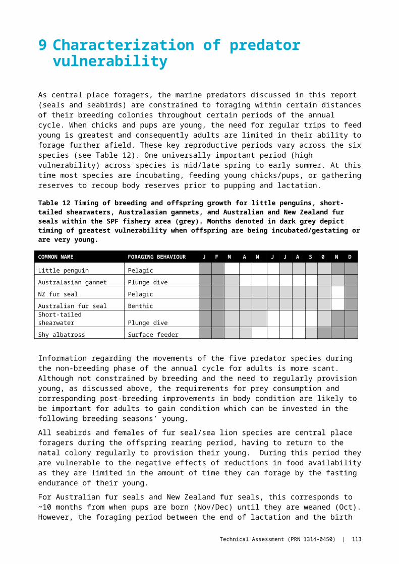
Smithers, B., D. Peck, A. Krockenberger, and B. Congdon. 2004. Elevated sea-surface temperature, reduced provisioning and reproductive failure of wedge-tailed shearwaters (Puffinus pacificus) in the southern Great Barrier Reef, Australia. Marine and Freshwater Research 54:973-977.
Staniland, I. J. 2002. Investigating the biases in the use of hard prey remains to identify diet composition using Antarctic fur seals (Arctocephalus gazella) in captive feeding trials. Marine Mammal Science 18:223-243.
Thompson, F. N., and E. R. Abraham. 2009. Estimation of the capture of New Zealand sea lions (Phocarctos hookeri) in trawl fisheries from 1995-96 to 2006-07. Ministry of Fisheries.
Thomson, R. B., D. S. Butterworth, I. L. Boyd, and J. P. Croxall. 2000. MODELING THE CONSEQUENCES OF ANTARCTIC KRILL HARVESTING ON ANTARCTIC FUR SEALS. Ecological Applications 10:1806-1819.
Tollit, D., S. Heaslip, B. Deagle, S. Iverson, R. Joy, D. Rosen, and A. Trites. 2006. Estimating diet composition in sea lions: Which technique to choose? Sea Lions of the World:293-307.
Tranquilla, L. M., A. Hedd, C. Burke, W. A. Montevecchi, P. M. Regular, G. J. Robertson, L. A. Stapleton, S. I. Wilhelm, D. A. Fifield, and A. D. Buren. 2010. High Arctic sea ice conditions influence marine birds wintering in Low Arctic regions. Estuarine Coastal and Shelf Science 89:97-106.
Trites, A. W., D. G. Calkins, and A. J. Winship. 2007. Diets of Steller sea lions (Eumetopias jubatus) in Southeast Alaska, 1993−1999. Fishery Bulletin 105:234-248.
Trites, A. W., and C. P. Donnelly. 2003. The decline of Steller sea lions Eumetopias jubatus in Alaska: a review of the nutritional stress hypothesis. Mammal Review 33:3-28.
Tuck, G. N., I. Knuckey, and N. L. Klaer. 2013. Informing the review of the Commonwealth Policy on Fisheries Bycatch through assessing trends in bycatch of key Commonwealth fisheries. FRDC 2012/046.
Venables, W. N., and B. D. Ripley. 2002. Modern applied statistics with S. Springer.Vincent, C., B. J. Mcconnell, V. Ridoux, and M. A. Fedak. 2002. Assessment of Argos location accuracy from
satellite tags deployed on captive gray seals. Marine Mammal Science 18:156-166.Wakefield, E. D., R. A. Phillips, and J. Matthiopoulos. 2009. Quantifying habitat use and preferences of
pelagic seabirds using individual movement data: a review. Marine Ecology Progress Series 391:165-182.
Wanless, S., M. Harris, P. Redman, and J. Speakman. 2005. Low energy values of fish as a probable cause of a major seabird breeding failure in the North Sea. Marine Ecology Progress Series 294:8.
Ward, T., A. Ivey, and P. Burch. 2011a. Spawning biomass of sardine, Sardinops sagax, in waters off South Australia in 2011.
Ward, T., J. Lyle, J. Keane, G. Begg, P. Hobsbawn, A. Ivey, R. Sakabe, and M. Steer. 2012. Commonwealth Small Pelagic Fishery: Fishery Assessment Report 2011. SARDI South Australian Research and Development Institute (Aquatic Sciences), Adelaide.
Ward, T. M., P. Burch, L. J. McLeay, and A. R. Ivey. 2011b. Use of the daily egg production method for stock assessment of sardine, Sardinops sagax; lessons learned over a decade of application off Southern Australia. Reviews in Fisheries Science 19:1-20.
Watkins, J. L., R. Hewitt, M. Naganobu, and V. Sushin. 2004. The CCAMLR 2000 Survey: a multinational, multi-ship biological oceanography survey of the Atlantic sector of the Southern Ocean. Deep Sea Research Part II: Topical Studies in Oceanography 51:1205-1213.
Watters, G. M., S. L. Hill, J. T. Hinke, J. Matthews, and K. Reid. 2013. Decision-making for ecosystem-based management: evaluating options for a krill fishery with an ecosystem dynamics model. Ecological Applications 23:710-725.
Weimerskirch, H., and Y. Cherel. 1998. Feeding ecology of short-tailed shearwaters: breeding in Tasmania and foraging in the Antarctic? Marine Ecology Progress Series 167:261-274.
Williams, T. M., J. A. Estes, D. F. Doak, and A. M. Springer. 2004. Killer appetites: assessing the role of predators in ecological communities. Ecology 85:3373-3384.
Wood, S. 2006. Generalized additive models: an introduction with R. CRC press.Wright, P. J., H. Jensen, H. Mosegaard, J. Dalskov, and S. Wanless. 2002. European Commission's annual
report on the impact of the Northeast sandeel fishery closure and status report on the monitoring fishery in 2000 and 2001.
114 | Technical Assessment (PRN 1314-0450)
Young, J., A. Jordan, C. Bobbi, R. Johannes, K. Haskard, and G. Pullen. 1993. Seasonal and interannual variability in krill (Nyctiphanes australis) stocks and their relationship to the fishery for jack mackerel (Trachurus declivis) off eastern Tasmania, Australia. Marine Biology 116:9-18.
Zucchini, W., and I. L. MacDonald. 2009. Hidden Markov models for time series: an introduction using R. CRC Press.
Technical Assessment (PRN 1314-0450) | 115
Appendix 1 Colony abundance size and distribution
Attached spreadsheet of colony abundance size and distribution.
116 | Technical Assessment (PRN 1314-0450)
Appendix 2 Diet data
Appendix 2A Diet data from various studies of SPF predators
This is contained in an electronic appendix
Appendix 2B Listings of percent biomass consumption data
Table A2.1 Percentage biomass consumption data used to calculate daily consumption for Australian fur seals.
Australian fur seal Body mass 76 kgPrey species Biomass contribution (%) Daily Consumption (g)Barracouta 30.4 3124.0Redbait 22.1 2271.1Arrow squid 8.5 873.5Jack mackerel 7.8 801.6Gurnard 7.1 729.6Bearded/Red cod 6.8 698.8Tiger flathead 6.6 678.2Silver trevally 2.1 215.8Calamari squid 1.8 185.0Leatherjacket 1.6 164.4Pink Ling 1.6 164.4Unknown sp1 1.2 123.3Western red mullet 0.9 92.5Silver Dory 0.4 41.1Maori Octopus 0.2 20.6Pale/keeled octopos 0.2 20.6Sand Flathead 0.2 20.6Silverside 0.2 20.6Silverbelly 0.1 10.3Anchovy 0.1 10.3
Total (g) 10266.1
Technical Assessment (PRN 1314-0450) | 117

Table A2.2 Percentage biomass consumption data used to calculate daily consumption for little penguins. Data extracted from (Chiaradia et al. 2012) for the years 1983-2006.
Little penguin Body mass 1.0 kgPrey species Biomass contribution (%) Daily Consumption (g)Anchovy (Engraulis australis) 22.0 62.6Pilchard (Sardinops sagax) 7.3 20.6Red Cod (Pseudophysis bachus) 8.0 22.8Barracouta (Thyrsites atun) 16.5 47.0Blue Warehou (Seriolella brama) 5.9 16.7Leatherjackets (Monocanthidae) 2.7 7.7Seahorses (Hippocampus sp.) 1.4 3.9Sandy Sprat (Hyperlochus vittatus) 0.1 0.2Hardyheads (Atherinason sp.) 0.3 0.9Red Bait (Emmelichthys nitidus) 0.4 1.1Jack Mackerel (Trachurus declivis) 0.4 1.1Garfish (Hemiramphus far) 0.5 1.4Gurnards (Triglidae) 0.5 1.4Red Mullet (Upeneichthys porosus) 0.7 2.0Pink Ling (Genypterus blacodes) 0.0 0.0Silver Warehou (Seriolella punctata) 0.3 0.7Trevallies (Carangidae) 0.1 0.2Fish postlarvae unknown 5.8 16.4Arrow squid (Nototodarus gouldi) 14.8 42.0Loliolus noctiluca 0.5 1.5Sepioteutis australis 0.1 0.2Argonauta nodosa 1.7 4.8Octopodidae 0.0 0.0Post Larvae Cephalopod 0.0 0.0Unknown Cephalopod 1.6 4.5Krill (Nyctiphanes australis) 5.7 16.2Stomatopoda 0.7 1.9Amphipoda 0.1 0.2Brachyura 0.0 0.0Megalopa 0.4 1.0Unknown Crustacea 0.0 0.0Other 1.7 4.7
Total (g) 284.0
118 | Technical Assessment (PRN 1314-0450)

Table A2.3 Percentage biomass consumption data used to calculate daily consumption for short tailed shearwaters. Data extracted from (Einoder et al. 2013b).
Short-tailed shearwater Body mass 0.620 kgPrey species Biomass contribution (%) Daily Consumption (g)Gould's squid (Nototodarus gouldi) 23.8 73.6Misc cephs (all <2% biomass) 4.3 13.4Coastal krill (Nyctiphanes australis) 39.0 120.5Sardinops sagax 1.4 4.4Jack mackeral Trachurus spp. 21.5 66.6Redbait Emmelichthys nitidus 1.0 3.0 Anchovy Engraulis australis 8.5 26.4Barracouta Thyrsites atun 0.4 1.3
Total (g) 309.2
Table A2.4 Percentage biomass consumption data used to calculate daily consumption for short tailed shearwaters. Data extracted from (Pyk et al. 2008).
Australasian gannet Body mass 2.6 kgPrey species Biomass contribution (%) Daily Consumption (g)Barracouta Thyrsites atun 27.8 163.9Redbait Emmelichthys nitidus 12.1 71.3Jack mackerel Trachurus declivis 36.6 215.8Anchovy Engraulis australis 4.9 28.9Red mullet Upenichthys vlamingii 7.9 46.6Pilchard Sardinops sagax 0.6 3.5Arrow squid Nototodarus gouldi 0.9 5.3Southern sea garfish Hyporhamphus melanochir 1.5 8.8Snapper Chrysophrys auratus 0.9 5.3Squid spp. 1.2 7.1Flathead spp. 0.7 4.1Trevalla Seriolella punctata 0.6 3.5Yellow-eye mullet Aldrichetta forsteri 0.5 2.9Black bream Acanthopagrus butcheri 1.0 5.9Unidentified 2.8 16.5Blue Mackerel Scomber australasicus 0.0 0.0
Total (g) 589.7
Technical Assessment (PRN 1314-0450) | 119
Appendix 3 Details of hidden Markov models for ARS categorization
Following Morales et al. (2004) we assume that the behavior of the animal is unobserved or hidden, but that it can be modeled using a Markov process on the states {C{T}} = {1,2} where state 1 is the Area restricted search state and state 2 is a directed transit movement state. Given data on the movements X{T} = {x1, …, xT} then we wish to obtain the likelihood of the data, in this case a bivariate time series of speeds and turn angles between locations, given the sequence of hidden states.
),Pr()Pr(}{
TTTTTT cxXxX CLm
CT
T (1)where
T
kkk
T
kkk cxcccC
2211 )|Pr()|Pr()Pr(),Pr( TTTT cxX
(2)The movement data for a given time are the step-length (speed) of the animal between times and the turning angle (i.e. the angle between subsequent movement vectors). We assume that the step length distribution is Weibull and the turning angles are distributed according to a Wrapped Cauchy distribution (Morales et al. 2004)
Stepk ~ Weibull(x, ai,bi) bb axabx exp1(3)
where x is the distance between subsequent locations, and
Turnk ~ Wrapped-Cauchy(ϕ, μi ,ρi) =
)cos(21
121
2
2
i
(4)
where ϕ is the angle between successive steps and the subscript i index the hidden state (ARS or Transit). We also need to estimate two transition parameters for the transition matrix πij = Pr(cik|cik-1); namely the Pr(ARSk | ARSk-1) and Pr(Transitk|Transitk-1). Note that Pr( Transitk| ARSk) = 1-Pr(ARSk|ARSk-1) and Pr(ARSk
|Transitk-1). Parameters ̂ = [πij , ai ,bi , ρi, μi] were estimated using the numerical Quasi-Newton minimization of (1) using the R function “optim”.
120 | Technical Assessment (PRN 1314-0450)
Appendix 4 Posterior simulation from GAMs
The following steps are required to sample from the posterior distributions of the GAM predictions. Having generated many of these draws, functions of these can be calculated with appropriate variances, which was used here to characterize spatial covariance in model predictions.
Let β̂ i are the estimated parameters of the GAM (smooth coefficients) and Σ̂i is their associated variance-covariance matrix. Then for simplicity, we assume that the posterior distribution of these parameters is multivariate Gaussian β i N ( β̂ i , Σ̂i ) then we can draw parameters from the posterior distributions on these parameters. These are used to predict time-spent as per the description above, but conditional on the newly drawn parameters. Again, from 1000 draws from the posterior distribution, an expected time spent in any given region was calculated labeled E(πr) and CV (πr).
Additionally for the delta-method calculations of spatial consumptions an approximate covariance matrix Σij describing the covariance between spatial blocks i and j was calculated by calculating the covariance across all sites. This matrix was inserted into the joint covariance of all parameters in the consumption model.
Technical Assessment (PRN 1314-0450) | 121

CONTACT USt 1300 363 400
+61 3 9545 2176e [email protected] www.csiro.au
YOUR CSIRO Australia is founding its future on science and innovation. Its national science agency, CSIRO, is a powerhouse of ideas, technologies and skills for building prosperity, growth, health and sustainability. It serves governments, industries, business and communities across the nation.
FOR FURTHER INFORMATIONCSIRO Oceans & Atmosphere FlagshipToby Pattersont +61 3 6232 45222e [email protected] www.csiro.au
122 | Technical Assessment (PRN 1314-0450)