Proximal Deep Structured Models

Shenlong WangUniversity of Toronto

slwang@cs.toronto.edu

Sanja FidlerUniversity of Toronto

fidler@cs.toronto.edu

Raquel UrtasunUniversity of Toronto

urtasun@cs.toronto.edu

Abstract

Many problems in real-world applications involve predicting continuous-valuedrandom variables that are statistically related. In this paper, we propose a powerfuldeep structured model that is able to learn complex non-linear functions whichencode the dependencies between continuous output variables. We show thatinference in our model using proximal methods can be efficiently solved as a feed-foward pass of a special type of deep recurrent neural network. We demonstratethe effectiveness of our approach in the tasks of image denoising, depth refinementand optical flow estimation.

1 Introduction

Many problems in real-world applications involve predicting a collection of random variables thatare statistically related. Over the past two decades, graphical models have been widely exploitedto encode these interactions in domains such as computer vision, natural language processing andcomputational biology. However, these models are shallow and only a log linear combination ofhand-crafted features is learned [40]. This limits the ability to learn complex patterns, which isparticularly important nowadays as large amounts of data are available, facilitating learning.

In contrast, deep learning approaches learn complex data abstractions by compositing simple non-linear transformations. In recent years, they have produced state-of-the-art results in many applica-tions such as speech recognition [17], object recognition [21], stereo estimation [44], and machinetranslation [38]. In some tasks, they have been shown to outperform humans, e.g., fine grainedcategorization [8] and object classification [15].

Deep neural networks are typically trained using simple loss functions. Cross entropy or hingeloss are used when dealing with discrete outputs, and squared loss when the outputs are continuous.Multi-task approaches are popular, where the hope is that dependencies of the output will be capturedby sharing intermediate layers among tasks [10].

Deep structured models attempt to learn complex features by taking into account the dependenciesbetween the output variables. A variety of methods have been developed in the context of predictingdiscrete outputs [8, 4, 34, 45]. Several techniques unroll inference and show how the forward andbackward passes of these deep structured models can be expressed as a set of standard layers [? ?34, 45]. This allows for fast end-to-end training on GPUs.

However, little to no attention has been given to deep structured models with continuous valuedoutput variables. One of the main reasons is that inference (even in the shallow model) is much lesswell studied, and very few solutions exist. An exception are Markov random fields (MRFs) withGaussian potentials, where exact inference is possible (via message-passing) if the precision matrix ispositive semi-definite and satisfies the spectral radius condition [42]. A family of popular approachesconvert the continuous inference problem into a discrete task using particle methods [18, 36]. Specificsolvers have also been designed for certain types of potentials, e.g. polynomials [41] and piecewiseconvex functions [43].

29th Conference on Neural Information Processing Systems (NIPS 2016), Barcelona, Spain.

Proximal methods are a popular solution to perform inference in continuous MRFs when the potentialsare non-smooth and non-differentiable functions of the outputs [27]. In this paper, we show thatproximal methods are a special type of recurrent neural networks. This allows us to efficiently train awide family of deep structured models with continuous output variables end-to-end on the GPU. Weshow that learning can simply be done via back-propagation for any differentiable loss function. Wedemonstrate the effectiveness of our algorithm in the tasks of image denoising, depth refinement andoptical flow and show superior results over competing algorithms on these tasks.

2 Proximal Deep Structured NetworksIn this section, we first introduce continuous-valued deep structured models and briefly reviewproximal methods. We then propose proximal deep structured models and discuss how to do efficientinference and learning in these models. Finally we discuss the relationship with previous work.

2.1 Continuous-valued Deep Structured ModelsGiven an input x ∈ X , let y = (y1, ..., yN ) be the set of random variables that we are interestedin predicting. The output space is a product space of all the elements: y ∈ Y =

∏Ni=1 Yi, and

the domain of each individual variable yi is a closed subset in real-valued space, i.e. Yi ⊂ R. LetE(x,y;w) : X × Y × RK → R be an energy function which encodes the problem that we areinterested in solving. Without loss of generality we assume that the energy decomposes into a sum offunctions, each depending on a subset of variables

E(x,y;w) =∑i

fi(yi,x;wu) +∑α

fα(yα,x;wα) (1)

where fi(yi;x,w) : Yi × X → R is a function that depends on a single variable (i.e., unary term)and fα(yα) : Yα × X → R depends on a subset of variables yα = (yi)i∈α defined on a domainYα ⊂ Y . Note that, unlike standard MRF models, the functions fi and fα are non-linear functions ofthe parameters.

The energy function is parameterized in terms of a set of weights w, and learning aims at finding thevalue of these weights which minimizes a loss function. Given an input x, inference aims at findingthe best configuration by minimizing the energy function:

y∗ = arg miny∈Y

∑i

fi(yi,x;wu) +∑α

fα(yα,x;wα) (2)

Finding the best scoring configuration y∗ is equivalent to maximizing the posteriori distribution:p(y|x;w) = 1

Z(x;w) exp(−E(x,y|w)), with Z(x;w) the partition function.

Standard multi-variate deep networks (e.g., FlowNet [12]) have potential functions which depend ona single output variable. In this simple case, inference corresponds to a forward pass that predicts thevalue of each variable independently. This can be interpreted as inference in a graphical model withonly unary potentials fi.

In the general case, performing inference in MRFs with continuous variables involves solvinga very challenging numerical optimization problem. Depending on the structure and propertiesof the potential functions, various methods have been proposed. For instance, particle methodsperform approximate inference by performing message passing on a series of discrete MRFs [18, 36].Exact inference is possible for a certain type of MRFs, i.e., Gaussian MRFs with positive semi-definite precision matrix. Efficient dedicated algorithms exist for a restricted family of functions,e.g., polynomials [41]. If certain conditions are satisfied, inference is often tackled by a group ofalgorithms called proximal methods [27]. In this section, we will focus on this family of inferencealgorithms and show that they are a particular type of recurrent net. We will use this fact to efficientlytrain deep structured models with continuous outputs.

2.2 A Review on Proximal MethodsNext, we briefly discuss proximal methods, and refer the reader to [27] for a thorough review.Proximal algorithms are very generally applicable, but they are particularly successful at solvingnon-smooth, non-differentiable, or constrained problems. Their base operation is evaluating theproximal operator of a function, which involves solving a small convex optimization problem that

2

often admits a closed-form solution. In particular, the proximal operator proxf (x0) : R→ R of afunction is defined as

proxf (x0) = arg miny

(y − x0)2 + f(y)

If f is convex, the fixed points of the proximal operator of f are precisely the minimizers of f . Inother words, proxf (x∗) = x∗ iff x∗ minimizes f . This fix-point property motivates the simplestproximal method called the proximal point algorithm which iterates x(n+1) = proxf (x(n)). All theproximal algorithms used here are based on this fix-point property. Note that even if the functionf(·) is not differentiable (e.g., `1 norm) there might exist a closed-form or easy to compute proximaloperator.

While the original proximal operator was designed for the purpose of obtaining the global optimumin convex optimization, recent work has shown that proximal methods work well for non-convexoptimization as long as the proximal operator exists [20, 33, 6].

For multi-variate optimization problems the proximal operator might not be trivial to obtain (e.g.,when having high-order potentials). In this case, a widely used solution is to decompose the high-order terms into small problems that can be solved through proximal operators. Examples of thisfamily of algorithms are half-quadratic splitting [14], alternating direction method of multipliers[13] and primal-dual methods [3] . In this work, we focus on the non-convex multi-variate case.

2.3 Proximal Deep Structured Models

In order to apply proximal algorithms to tackle the inference problem defined in Eq. (2), we requirethe energy functions fi and fα to satisfy the following conditions:

1. There exist functions hi and gi such that fi(yi,x;w) = gi(yi, hi(x,w)), where gi is adistance function 1;

2. There exists a closed-form proximal operator for gi(yi, hi(x;w)) wrt yi.

3. There exist functions hα and gα such that fα(yα,x;w) can be re-written as fα(yα,x;w) =hα(x;w)gα(wT

αyα).

4. There exists a proximal operator for either the dual or primal form of gα(·).

A fairly general family of deep structured models satisfies these conditions. Our experimentalevaluation will demonstrate the applicability in a wide variety of tasks including depth refinement,image denoising as well as optical flow. If our potential functions satisfy the conditions above, wecan rewrite our objective function as follows:

E(x,y;w) =∑i

gi(yi, hi(x;w)) +∑α

hα(x;w)gα(wTαyα) (3)

In this paper, we make the important observation that each iteration of most existing proximal solverscontain five sub-steps: (i) compute the locally linear part; (ii) compute the proximal operator proxgi ;(iii) deconvolve; (iv) compute the proximal operator proxgα ; (v) update the result through a gradientdescent step. Due to space restrictions, we show primal-dual solvers in this section, and refer thereader to the supplementary material for ADMM, half-quadratic splitting and the proximal gradientmethod.

The general idea of primal dual solvers is to introduce auxiliary variables z to decompose the high-order terms. We can then minimize z and y alternately through computing their proximal operator.In particular, we can transform the primal problem in Eq. (3) into the following saddle point problem

miny∈Y

maxz∈Z

∑i

gi(yi, hi(x,wu))−∑α

hα(x,w)g∗α(zα) +∑α

hα(x,w)〈wTαyα, zα〉 (4)

where g∗α(·) is the convex conjugate of gα(·): g∗α(z∗) = sup{〈z∗, z〉 − gα(z)|z ∈ Z} and the convexconjugate of g∗α is gα itself, if gα(·) is convex.

1A function g : Y × Y → [0,∞) is called a distance function iff it satisfies the condition of non-negativity,identity of indisernibles, symmetry and triangle inequality.

3

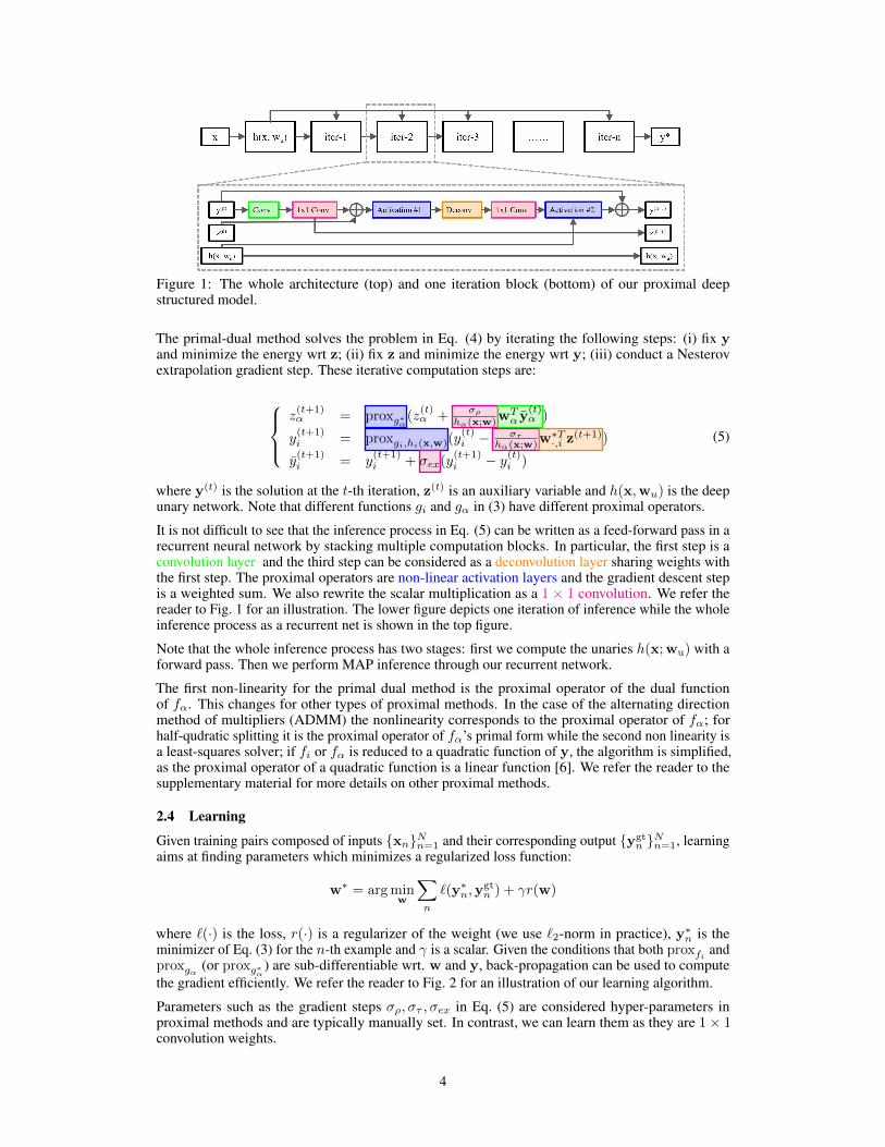
Figure 1: The whole architecture (top) and one iteration block (bottom) of our proximal deepstructured model.

The primal-dual method solves the problem in Eq. (4) by iterating the following steps: (i) fix yand minimize the energy wrt z; (ii) fix z and minimize the energy wrt y; (iii) conduct a Nesterovextrapolation gradient step. These iterative computation steps are:

z(t+1)α = proxg∗α(z

(t)α +

σρhα(x;w)w

Tα y

(t)α )

y(t+1)i = proxgi,hi(x,w)(y

(t)i −

στhα(x;w)w

∗T·,i z

(t+1))

y(t+1)i = y

(t+1)i + σex(y

(t+1)i − y(t)i )

(5)

where y(t) is the solution at the t-th iteration, z(t) is an auxiliary variable and h(x,wu) is the deepunary network. Note that different functions gi and gα in (3) have different proximal operators.

It is not difficult to see that the inference process in Eq. (5) can be written as a feed-forward pass in arecurrent neural network by stacking multiple computation blocks. In particular, the first step is aconvolution layer and the third step can be considered as a deconvolution layer sharing weights withthe first step. The proximal operators are non-linear activation layers and the gradient descent stepis a weighted sum. We also rewrite the scalar multiplication as a 1 × 1 convolution. We refer thereader to Fig. 1 for an illustration. The lower figure depicts one iteration of inference while the wholeinference process as a recurrent net is shown in the top figure.

Note that the whole inference process has two stages: first we compute the unaries h(x;wu) with aforward pass. Then we perform MAP inference through our recurrent network.

The first non-linearity for the primal dual method is the proximal operator of the dual functionof fα. This changes for other types of proximal methods. In the case of the alternating directionmethod of multipliers (ADMM) the nonlinearity corresponds to the proximal operator of fα; forhalf-qudratic splitting it is the proximal operator of fα’s primal form while the second non linearity isa least-squares solver; if fi or fα is reduced to a quadratic function of y, the algorithm is simplified,as the proximal operator of a quadratic function is a linear function [6]. We refer the reader to thesupplementary material for more details on other proximal methods.

2.4 Learning

Given training pairs composed of inputs {xn}Nn=1 and their corresponding output {ygtn }Nn=1, learning

aims at finding parameters which minimizes a regularized loss function:

w∗ = arg minw

∑n

`(y∗n,ygtn ) + γr(w)

where `(·) is the loss, r(·) is a regularizer of the weight (we use `2-norm in practice), y∗n is theminimizer of Eq. (3) for the n-th example and γ is a scalar. Given the conditions that both proxfi andproxgα (or proxg∗α) are sub-differentiable wrt. w and y, back-propagation can be used to computethe gradient efficiently. We refer the reader to Fig. 2 for an illustration of our learning algorithm.

Parameters such as the gradient steps σρ, στ , σex in Eq. (5) are considered hyper-parameters inproximal methods and are typically manually set. In contrast, we can learn them as they are 1× 1convolution weights.

4

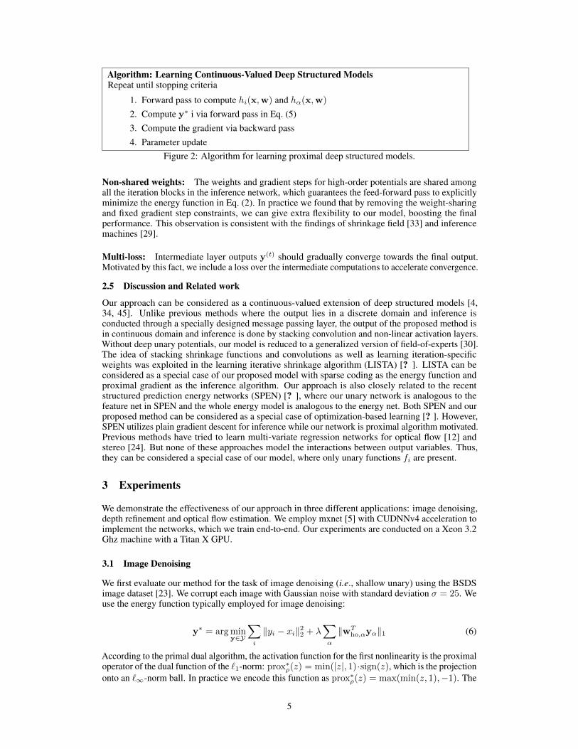
Algorithm: Learning Continuous-Valued Deep Structured ModelsRepeat until stopping criteria

1. Forward pass to compute hi(x,w) and hα(x,w)

2. Compute y∗ i via forward pass in Eq. (5)3. Compute the gradient via backward pass4. Parameter update

Figure 2: Algorithm for learning proximal deep structured models.

Non-shared weights: The weights and gradient steps for high-order potentials are shared amongall the iteration blocks in the inference network, which guarantees the feed-forward pass to explicitlyminimize the energy function in Eq. (2). In practice we found that by removing the weight-sharingand fixed gradient step constraints, we can give extra flexibility to our model, boosting the finalperformance. This observation is consistent with the findings of shrinkage field [33] and inferencemachines [29].

Multi-loss: Intermediate layer outputs y(t) should gradually converge towards the final output.Motivated by this fact, we include a loss over the intermediate computations to accelerate convergence.

2.5 Discussion and Related work

Our approach can be considered as a continuous-valued extension of deep structured models [4,34, 45]. Unlike previous methods where the output lies in a discrete domain and inference isconducted through a specially designed message passing layer, the output of the proposed method isin continuous domain and inference is done by stacking convolution and non-linear activation layers.Without deep unary potentials, our model is reduced to a generalized version of field-of-experts [30].The idea of stacking shrinkage functions and convolutions as well as learning iteration-specificweights was exploited in the learning iterative shrinkage algorithm (LISTA) [? ]. LISTA can beconsidered as a special case of our proposed model with sparse coding as the energy function andproximal gradient as the inference algorithm. Our approach is also closely related to the recentstructured prediction energy networks (SPEN) [? ], where our unary network is analogous to thefeature net in SPEN and the whole energy model is analogous to the energy net. Both SPEN and ourproposed method can be considered as a special case of optimization-based learning [? ]. However,SPEN utilizes plain gradient descent for inference while our network is proximal algorithm motivated.Previous methods have tried to learn multi-variate regression networks for optical flow [12] andstereo [24]. But none of these approaches model the interactions between output variables. Thus,they can be considered a special case of our model, where only unary functions fi are present.

3 Experiments

We demonstrate the effectiveness of our approach in three different applications: image denoising,depth refinement and optical flow estimation. We employ mxnet [5] with CUDNNv4 acceleration toimplement the networks, which we train end-to-end. Our experiments are conducted on a Xeon 3.2Ghz machine with a Titan X GPU.

3.1 Image Denoising

We first evaluate our method for the task of image denoising (i.e., shallow unary) using the BSDSimage dataset [23]. We corrupt each image with Gaussian noise with standard deviation σ = 25. Weuse the energy function typically employed for image denoising:

y∗ = arg miny∈Y

∑i

‖yi − xi‖22 + λ∑α

‖wTho,αyα‖1 (6)

According to the primal dual algorithm, the activation function for the first nonlinearity is the proximaloperator of the dual function of the `1-norm: prox∗ρ(z) = min(|z|, 1)·sign(z), which is the projectiononto an `∞-norm ball. In practice we encode this function as prox∗ρ(z) = max(min(z, 1),−1). The

5

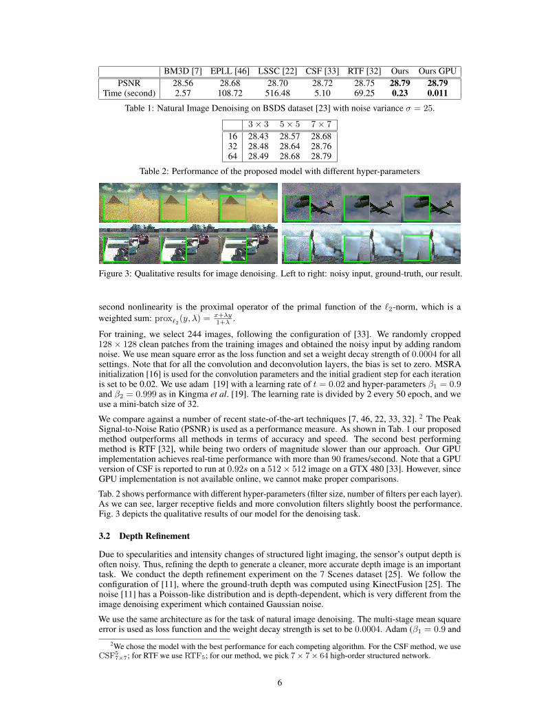
BM3D [7] EPLL [46] LSSC [22] CSF [33] RTF [32] Ours Ours GPUPSNR 28.56 28.68 28.70 28.72 28.75 28.79 28.79

Time (second) 2.57 108.72 516.48 5.10 69.25 0.23 0.011

Table 1: Natural Image Denoising on BSDS dataset [23] with noise variance σ = 25.

3× 3 5× 5 7× 7

16 28.43 28.57 28.6832 28.48 28.64 28.7664 28.49 28.68 28.79

Table 2: Performance of the proposed model with different hyper-parameters

Figure 3: Qualitative results for image denoising. Left to right: noisy input, ground-truth, our result.

second nonlinearity is the proximal operator of the primal function of the `2-norm, which is aweighted sum: prox`2(y, λ) = x+λy

1+λ .

For training, we select 244 images, following the configuration of [33]. We randomly cropped128× 128 clean patches from the training images and obtained the noisy input by adding randomnoise. We use mean square error as the loss function and set a weight decay strength of 0.0004 for allsettings. Note that for all the convolution and deconvolution layers, the bias is set to zero. MSRAinitialization [16] is used for the convolution parameters and the initial gradient step for each iterationis set to be 0.02. We use adam [19] with a learning rate of t = 0.02 and hyper-parameters β1 = 0.9and β2 = 0.999 as in Kingma et al. [19]. The learning rate is divided by 2 every 50 epoch, and weuse a mini-batch size of 32.

We compare against a number of recent state-of-the-art techniques [7, 46, 22, 33, 32]. 2 The PeakSignal-to-Noise Ratio (PSNR) is used as a performance measure. As shown in Tab. 1 our proposedmethod outperforms all methods in terms of accuracy and speed. The second best performingmethod is RTF [32], while being two orders of magnitude slower than our approach. Our GPUimplementation achieves real-time performance with more than 90 frames/second. Note that a GPUversion of CSF is reported to run at 0.92s on a 512× 512 image on a GTX 480 [33]. However, sinceGPU implementation is not available online, we cannot make proper comparisons.

Tab. 2 shows performance with different hyper-parameters (filter size, number of filters per each layer).As we can see, larger receptive fields and more convolution filters slightly boost the performance.Fig. 3 depicts the qualitative results of our model for the denoising task.

3.2 Depth Refinement

Due to specularities and intensity changes of structured light imaging, the sensor’s output depth isoften noisy. Thus, refining the depth to generate a cleaner, more accurate depth image is an importanttask. We conduct the depth refinement experiment on the 7 Scenes dataset [25]. We follow theconfiguration of [11], where the ground-truth depth was computed using KinectFusion [25]. Thenoise [11] has a Poisson-like distribution and is depth-dependent, which is very different from theimage denoising experiment which contained Gaussian noise.

We use the same architecture as for the task of natural image denoising. The multi-stage mean squareerror is used as loss function and the weight decay strength is set to be 0.0004. Adam (β1 = 0.9 and

2We chose the model with the best performance for each competing algorithm. For the CSF method, we useCSF5

7×7; for RTF we use RTF5; for our method, we pick 7× 7× 64 high-order structured network.

6

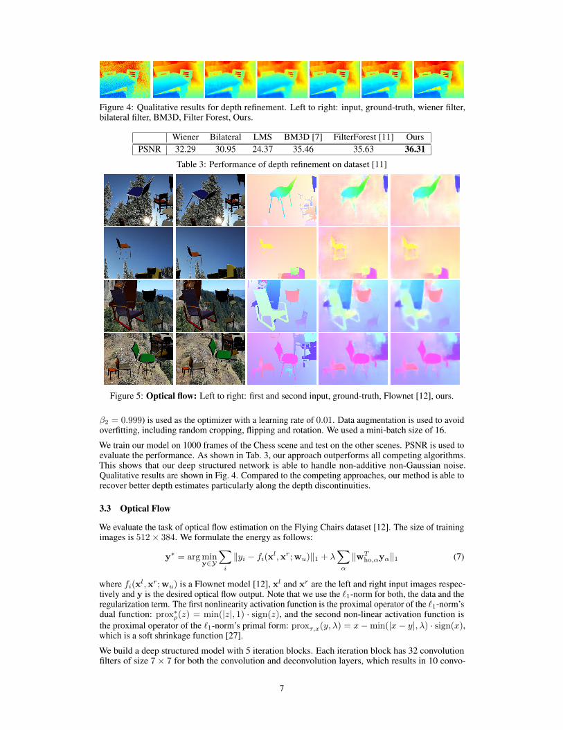
Figure 4: Qualitative results for depth refinement. Left to right: input, ground-truth, wiener filter,bilateral filter, BM3D, Filter Forest, Ours.

Wiener Bilateral LMS BM3D [7] FilterForest [11] OursPSNR 32.29 30.95 24.37 35.46 35.63 36.31

Table 3: Performance of depth refinement on dataset [11]

Figure 5: Optical flow: Left to right: first and second input, ground-truth, Flownet [12], ours.

β2 = 0.999) is used as the optimizer with a learning rate of 0.01. Data augmentation is used to avoidoverfitting, including random cropping, flipping and rotation. We used a mini-batch size of 16.

We train our model on 1000 frames of the Chess scene and test on the other scenes. PSNR is used toevaluate the performance. As shown in Tab. 3, our approach outperforms all competing algorithms.This shows that our deep structured network is able to handle non-additive non-Gaussian noise.Qualitative results are shown in Fig. 4. Compared to the competing approaches, our method is able torecover better depth estimates particularly along the depth discontinuities.

3.3 Optical Flow

We evaluate the task of optical flow estimation on the Flying Chairs dataset [12]. The size of trainingimages is 512× 384. We formulate the energy as follows:

y∗ = arg miny∈Y

∑i

‖yi − fi(xl,xr;wu)‖1 + λ∑α

‖wTho,αyα‖1 (7)

where fi(xl,xr;wu) is a Flownet model [12], xl and xr are the left and right input images respec-tively and y is the desired optical flow output. Note that we use the `1-norm for both, the data and theregularization term. The first nonlinearity activation function is the proximal operator of the `1-norm’sdual function: prox∗ρ(z) = min(|z|, 1) · sign(z), and the second non-linear activation function isthe proximal operator of the `1-norm’s primal form: proxτ,x(y, λ) = x−min(|x− y|, λ) · sign(x),which is a soft shrinkage function [27].

We build a deep structured model with 5 iteration blocks. Each iteration block has 32 convolutionfilters of size 7 × 7 for both the convolution and deconvolution layers, which results in 10 convo-

7

Flownet Flownet + TV-l1 Our proposedEnd-point-error 4.98 4.96 4.91

Table 4: Performance of optical flow on Flying chairs dataset [12]

lution/deconv layers and 10 non-linearities. The multi-stage mean square error is used as the lossfunction and the weight decay strength is set to be 0.0004.

Training is conducted on the training subset of the Flying Chairs dataset. Our unary model isinitialized with a pre-trained Flownet parameters. The high-order term is initialized with MSRArandom initialization [16]. The hyper-parameter λ in this experiment is pre-set to be 10. We userandom flipping, cropping and color-tuning for data augmentation, and employ the adam optimizerwith the same configuration as before (β1 = 0.9 and β2 = 0.999) with a learning rate t = 0.005. Thelearning rate is divided by 2 every 10 epoch and the mini-batch size is set to be 12.

We evaluate all approaches on the test set of the Flying chairs dataset. End-point error is used asa measure of performance. The unary-only model (i.e. plain flownet) is used as baseline and wealso compare against a plain TV-l1 model with four pre-set gradient operator as post-processing. Asshown in Tab. 4 our method outperforms all the baselines. From Fig. 5 we can see that our method isless noisy than Flownet’s output and better preserves the boundaries. Note that our current model isisotropic. In order to further boost the performance, incorporating anisotropic filtering like bilateralfiltering is an interesting future direction.

4 Conclusion

We have proposed a deep structured model that learns non-linear functions encoding complexdependencies between continuous output variables. We have showed that inference in our modelusing proximal methods can be efficiently solved as a feed-foward pass on a special type of deeprecurrent neural network. We demonstrated our approach in the tasks of image denoising, depthrefinement and optical flow. In the future we plan to investigate other proximal methods and a widervariety of applications.

References[1] Frederic Besse, Carsten Rother, Andrew Fitzgibbon, and Jan Kautz. Pmbp: Patchmatch belief propagation

for correspondence field estimation. IJCV, 2014.

[2] Harold C Burger, Christian J Schuler, and Stefan Harmeling. Image denoising: Can plain neural networkscompete with bm3d? In CVPR, pages 2392–2399. IEEE, 2012.

[3] Antonin Chambolle and Thomas Pock. A first-order primal-dual algorithm for convex problems withapplications to imaging. Journal of Mathematical Imaging and Vision, 2011.

[4] Liang-chieh Chen, Alexander Schwing, Alan Yuille, and Raquel Urtasun. Learning deep structured models.In ICML, 2015.

[5] Tianqi Chen, Mu Li, Yutian Li, Min Lin, Naiyan Wang, Minjie Wang, Tianjun Xiao, Bing Xu, ChiyuanZhang, and Zheng Zhang. Mxnet: A flexible and efficient machine learning library for heterogeneousdistributed systems. arXiv preprint arXiv:1512.01274, 2015.

[6] Yunjin Chen, Wei Yu, and Thomas Pock. On learning optimized reaction diffusion processes for effectiveimage restoration. In CVPR, 2015.

[7] Kostadin Dabov, Alessandro Foi, Vladimir Katkovnik, and Karen Egiazarian. Image denoising by sparse3-d transform-domain collaborative filtering. TIP, 2007.

[8] Jia Deng, Nan Ding, Yangqing Jia, Andrea Frome, Kevin Murphy, Samy Bengio, Yuan Li, Hartmut Neven,and Hartwig Adam. Large-scale object classification using label relation graphs. In ECCV. 2014.

[9] Chao Dong, Chen Change Loy, Kaiming He, and Xiaoou Tang. Learning a deep convolutional network forimage super-resolution. In ECCV. 2014.

[10] David Eigen and Rob Fergus. Predicting depth, surface normals and semantic labels with a commonmulti-scale convolutional architecture. In ICCV, pages 2650–2658, 2015.

8

[11] Sean Fanello, Cem Keskin, Pushmeet Kohli, Shahram Izadi, Jamie Shotton, Antonio Criminisi, UgoPattacini, and Tim Paek. Filter forests for learning data-dependent convolutional kernels. In CVPR, 2014.

[12] Philipp Fischer, Alexey Dosovitskiy, Eddy Ilg, Philip Häusser, Caner Hazırbas, Vladimir Golkov, Patrickvan der Smagt, Daniel Cremers, and Thomas Brox. Flownet: Learning optical flow with convolutionalnetworks. In CVPR, 2015.

[13] Daniel Gabay and Bertrand Mercier. A dual algorithm for the solution of nonlinear variational problemsvia finite element approximation. Computers & Mathematics with Applications, 1976.

[14] Donald Geman and Chengda Yang. Nonlinear image recovery with half-quadratic regularization. ImageProcessing, IEEE Transactions on, 4(7):932–946, 1995.

[15] Kaiming He, Xiangyu Zhang, Shaoqing Ren, and Jian Sun. Deep residual learning for image recognition.arXiv preprint arXiv:1512.03385, 2015.

[16] Kaiming He, Xiangyu Zhang, Shaoqing Ren, and Jian Sun. Delving deep into rectifiers: Surpassinghuman-level performance on imagenet classification. In ICCV, 2015.

[17] Geoffrey Hinton, Li Deng, Dong Yu, George E Dahl, Abdel-rahman Mohamed, Navdeep Jaitly, AndrewSenior, Vincent Vanhoucke, Patrick Nguyen, Tara N Sainath, et al. Deep neural networks for acousticmodeling in speech recognition: The shared views of four research groups. Signal Processing Magazine,IEEE, 2012.

[18] Alexander T Ihler and David A McAllester. Particle belief propagation. In AISTATS, 2009.

[19] Diederik Kingma and Jimmy Ba. Adam: A method for stochastic optimization. arXiv preprintarXiv:1412.6980, 2014.

[20] Dilip Krishnan and Rob Fergus. Fast image deconvolution using hyper-laplacian priors. In NIPS, 2009.

[21] Alex Krizhevsky, Ilya Sutskever, and Geoffrey E Hinton. Imagenet classification with deep convolutionalneural networks. In NIPS, 2012.

[22] Julien Mairal, Francis Bach, Jean Ponce, Guillermo Sapiro, and Andrew Zisserman. Non-local sparsemodels for image restoration. In ICCV, 2009.

[23] David Martin, Charless Fowlkes, Doron Tal, and Jitendra Malik. A database of human segmented naturalimages and its application to evaluating segmentation algorithms and measuring ecological statistics. InICCV, 2001.

[24] Nikolaus Mayer, Eddy Ilg, Philip Häusser, Philipp Fischer, Daniel Cremers, Alexey Dosovitskiy, andThomas Brox. A large dataset to train convolutional networks for disparity, optical flow, and scene flowestimation. arXiv preprint arXiv:1512.02134, 2015.

[25] Richard A Newcombe, Shahram Izadi, Otmar Hilliges, David Molyneaux, David Kim, Andrew J Davison,Pushmeet Kohi, Jamie Shotton, Steve Hodges, and Andrew Fitzgibbon. Kinectfusion: Real-time densesurface mapping and tracking. In ISMAR, 2011.

[26] Sebastian Nowozin and Christoph H Lampert. Structured learning and prediction in computer vision.Foundations and Trends R© in Computer Graphics and Vision, 6(3–4):185–365, 2011.

[27] Neal Parikh and Stephen P Boyd. Proximal algorithms. Foundations and Trends in optimization, 1(3):127–239, 2014.

[28] Emilio Parisotto, Jimmy Lei Ba, and Ruslan Salakhutdinov. Actor-mimic: Deep multitask and transferreinforcement learning. arXiv preprint arXiv:1511.06342, 2015.

[29] Stephane Ross, Daniel Munoz, Martial Hebert, and J Andrew Bagnell. Learning message-passing inferencemachines for structured prediction. In CVPR, 2011.

[30] Stefan Roth and Michael J Black. Fields of experts: A framework for learning image priors. In CVPR,2005.

[31] Mathieu Salzmann. Continuous inference in graphical models with polynomial energies. In Proceedingsof the IEEE Conference on Computer Vision and Pattern Recognition, pages 1744–1751, 2013.

[32] Uwe Schmidt, Jeremy Jancsary, Sebastian Nowozin, Stefan Roth, and Carsten Rother. Cascades ofregression tree fields for image restoration. PAMI, 2013.

9

[33] Uwe Schmidt and Stefan Roth. Shrinkage fields for effective image restoration. In CVPR, 2014.

[34] Alexander G Schwing and Raquel Urtasun. Fully connected deep structured networks. arXiv preprintarXiv:1503.02351, 2015.

[35] Jamie Shotton, Ben Glocker, Christopher Zach, Shahram Izadi, Antonio Criminisi, and Andrew Fitzgibbon.Scene coordinate regression forests for camera relocalization in rgb-d images. In CVPR, 2013.

[36] Erik B Sudderth, Alexander T Ihler, Michael Isard, William T Freeman, and Alan S Willsky. Nonparametricbelief propagation. Communications of the ACM, 2010.

[37] Sainbayar Sukhbaatar, Arthur Szlam, Jason Weston, and Rob Fergus. End-to-end memory networks. 2015.

[38] Ilya Sutskever, Oriol Vinyals, and Quoc V Le. Sequence to sequence learning with neural networks. InNIPS, 2014.

[39] Yaniv Taigman, Ming Yang, Marc’Aurelio Ranzato, and Lior Wolf. Deepface: Closing the gap tohuman-level performance in face verification. In CVPR, 2014.

[40] Ioannis Tsochantaridis, Thomas Hofmann, Thorsten Joachims, and Yasemin Altun. Support vector machinelearning for interdependent and structured output spaces. In ICML, 2004.

[41] Shenlong Wang, Alex Schwing, and Raquel Urtasun. Efficient inference of continuous markov randomfields with polynomial potentials. In Advances in neural information processing systems, pages 936–944,2014.

[42] Yair Weiss and William T Freeman. Correctness of belief propagation in gaussian graphical models ofarbitrary topology. Neural computation, 2001.

[43] Christopher Zach and Pushmeet Kohli. A convex discrete-continuous approach for markov random fields.In ECCV. 2012.

[44] Jure Zbontar and Yann LeCun. Computing the stereo matching cost with a convolutional neural network.In CVPR, 2015.

[45] Shuai Zheng, Sadeep Jayasumana, Bernardino Romera-Paredes, Vibhav Vineet, Zhizhong Su, Dalong Du,Chang Huang, and Philip HS Torr. Conditional random fields as recurrent neural networks. In ICCV, 2015.

[46] Daniel Zoran and Yair Weiss. From learning models of natural image patches to whole image restoration.In ICCV, 2011.

10