Proximity and Investment:

Evidence from Plant-Level Data∗

Xavier Giroud†

September 2011

Abstract

Proximity to plants makes it easier for headquarters to monitor and acquire information

about plants. In this paper, I estimate the effects of headquarters’ proximity to plants on

plant investment and productivity. Using the introduction of new airline routes as a source

of exogenous variation in proximity, I find that new airline routes that reduce the travel time

between headquarters and plants lead to an increase in plant investment of 8% to 9% and

to an increase in plants’ total factor productivity of 1.3% to 1.4%. The results are robust

to controlling for local and firm-level shocks that could potentially cause the introduction

of new airlines routes, they are robust when I consider only new airline routes that are the

outcome of a merger between two airlines or the opening of a new hub, and they are robust

when I consider only indirect flights where either the last leg of the flight (involving the

plant’s home base airport) or the first leg of the flight (involving headquarters’ home base

airport) remains unchanged.

∗This paper is based on my dissertation submitted to New York University. I am grateful to my advisor, HolgerMueller, as well as to Viral Acharya, Ashwini Agrawal, Allan Collard-Wexler, Carola Frydman, Xavier Gabaix,

Kose John, Marcin Kacperczyk, Andrew Karolyi, Leonid Kogan, Anthony Lynch, Javier Miranda, Adair Morse,

Dimitris Papanikolaou, Adriano Rampini, Michael Roberts, Alexi Savov, Philipp Schnabl, Antoinette Schoar,

Amit Seru, Daniel Wolfenzon, and seminar participants at MIT, Chicago, Stanford, NYU, Wharton, Kellogg,

UCLA, Yale, Duke, Ohio State, Cornell, and USC for valuable comments and suggestions. The research in this

paper was conducted while the author was a Special Sworn Status researcher of the U.S. Census Bureau at the

New York Census Research Data Center. Any opinions and conclusions expressed herein are those of the author

and do not necessarily represent the views of the U.S. Census Bureau. All results have been reviewed to ensure

that no confidential information is disclosed.†MIT Sloan School of Management. Email: xgiroud@mit.edu.

1This is a pre-copyedited, author-produced version of an article accepted for publication in The Quarterly Journal of Economics following peer review. The version of record [Giroud, Xavier. "Proximity and Investment: Evidence from Plant-Level Data." The Quarterly Journal of Economics 128, no. 2 (2013): 861-915] is available online at: https://doi.org/10.1093/qje/qjs073

1 Introduction

Proximity facilitates monitoring and access to information. For instance, venture capitalists

are more likely to serve on the boards of local firms, where monitoring is easier (Lerner, 1995).

Likewise, mutual fund managers are more likely to hold shares of local firms–and they earn

substantial abnormal returns from these investments–suggesting “improved monitoring capabil-

ities or access to private information of geographically proximate firms” (Coval and Moskowitz,

1999, 2001 (p. 812)). Finally, banks located closer to their borrowers are more likely to lend to

informationally difficult borrowers, e.g., borrowers without any financial records (Petersen and

Rajan, 2002; Mian, 2006; Sufi, 2007).

All of the above examples come from arm’s length transactions. Much less, if anything, is

known about the role of proximity within firms. For instance, is it true that–in analogy to the

empirical findings in the mutual funds and banking literatures–headquarters is more likely to

invest in plants that are located closer to headquarters? And does proximity to headquarters

improve plant productivity? Understanding plant investment and productivity is important, not

the least because they affect economic growth.1 One difficulty in answering these questions is

that they require data on the locations of plants and headquarters. Another, more serious issue

is that the locations of plants and headquarters are choice variables. Accordingly, commonly

used proxies for proximity–such as the physical distance between plants and headquarters–are

likely to be endogenous, making it difficult to establish causality.

In this paper, I attempt to address both of these issues. As for the first issue, I use plant-level

data provided by the U.S. Census Bureau for the manufacturing sector for the period 1977 to

2005, which include the locations of plants and headquarters. As for the second issue, I notice

that the main reason why empirical studies are interested in (geographical) proximity is because

it proxies for the ease of monitoring and acquiring information. I argue that a more direct proxy

is travel time. For instance, a plant may be located far away from headquarters, yet monitoring

may be easy, because there exists a short, direct flight. Conversely, a plant may be located in the

1Anecdotal evidence suggests that proximity to headquarters is a potentially important determinant of plant

investment. For instance, when Tesla Motors decided on the location of a manufacturing plant to produce its

electric Tesla roadster, it announced that the plant would be located “as close to our headquarters as possible,”

citing as a reason “to keep better control over production” (Silicon Valley/San Jose Business Journal, June

30, 2008). As for the effects of proximity on productivity, Ray Kroc, the founder of McDonald’s, writes in

his autobiography: “One thing I liked about that house was that it was perched on a hill looking down on a

McDonald’s store on the main thoroughfare. I could pick up a pair of binoculars and watch business in that store

from my living room window. It drove the manager crazy when I told him about it. But he sure had one hell of

a hard-working crew!” (Kroc, 1992, p. 141).

2

same state as headquarters, yet monitoring may be costly, because it involves a long and tedious

road trip. Of course, in the cross-section, geographical proximity and travel time are highly

correlated. However, the advantage of using travel time is that it entails plausibly exogenous

variation, allowing me to address the endogeneity issue.

Specifically, I combine the Census plant-level data with airline data from the U.S. Department

of Transportation, which contain information about all flights that have taken place between

any two airports in the U.S. The source of exogenous variation that I exploit is the introduction

of new airline routes that reduce the travel time between headquarters and plants. Using a

difference-in-differences approach, I find that the introduction of new airline routes leads to an

increase in plant investment of 8% to 9%, corresponding to an increase in capital expenditures

of $213,000 to $239,000 (in 1997 dollars). Moreover, I find that plants’ total factor productivity

increases by 1.3% to 1.4%, corresponding to an increase in plant profits of $67,000 to $93,000

(in 1997 dollars). In both cases, the effect is stronger for larger reductions in travel time, and it

is only significant for travel time reductions of at least two hours round trip.

My identification strategy can be illustrated with a simple example. Consider a company

with headquarters in Boston and a plant in Memphis. In 1985, the fastest way to travel from

Boston to Memphis was an indirect flight with one stopover in Atlanta. In 1986, Northwest

Airlines opened a new hub in Memphis and started operating direct flights between Boston and

Memphis. The introduction of this new airline route substantially reduced the travel between

the Boston headquarters and the Memphis plant and is coded as a “treatment” of the Memphis

plant.2 To measure the effect of this treatment on, e.g., investment, one could simply compare

investment at the Memphis plant before and after 1986. However, other events in 1986 might

have also affected investment at the Memphis plant. For instance, there might have been a

nationwide surge in investment due to favorable economic conditions or low interest rates. To

account for this possibility, I include a control group that consists of all plants that have not

(yet) been treated. I then compare the difference in investment at the Memphis plant before

and after 1986 with the difference in investment at the control plants before and after 1986.

The difference between the two differences is the estimated effect of the introduction of the new

airline route between Boston and Memphis on investment at the Memphis plant.

An important concern is that local shocks in the plants’ vicinity or firm-level shocks could

2Overall, there are 10,533 plants in my sample that experience a reduction in the travel time to headquarters

due to the introduction of new airline routes.

3

be driving both the introduction of new airline routes and plant investment. For instance,

suppose the Memphis area experiences an economic boom. As the local economy is booming,

the company headquartered in Boston may find it more attractive to increase investment at the

Memphis plant. At the same time, airlines may find it more attractive to introduce new flights

to Memphis. In this case, finding a positive treatment effect would be a spurious outcome of

an omitted shock in the Memphis area. Likewise, it is easy to construct examples in which an

omitted firm-level shock gives rise to a spurious treatment effect.

Given that omitted local and firm-level shocks can lead to spurious treatment effects, it

is important to control for such shocks. Since a treatment is uniquely defined by two (air-

port) locations–the locations of the plant’s and headquarters’ airports–I can do this, making

the identification tighter. Specifically, I include MSA-year and firm-year controls in all my re-

gressions. Both types of controls are identified here, because not all local plants have their

headquarters in the same city or region, and because not all plants of a company are affected

by the introduction of a new airline route.

While the inclusion of MSA- and firm-year controls accounts for the possibility of omitted

local and firm-level shocks, it remains the possibility of an omitted shock that is specific to a

single plant–i.e., the shock does not affect other plants in the same region. In response to

this shock, headquarters may increase investment at the plant. At the same time, the plant

may lobby for the introduction of a new airline route to its headquarters. Unlike the local

and firm-level shocks described above, such plant-specific shocks–provided they lead to the

introduction of a new airline route to headquarters–are collinear with the treatment. Hence,

neither MSA-year controls nor firm-year controls can account for them.

I address this issue in three different ways. First, I consider the dynamic effects of the

introduction of new airline routes. If a new airline route is the (endogenous) outcome of a pre-

existing plant-specific shock, then I should find an “effect” of the treatment already before the

new airline route is introduced. However, I find no such effect. On the contrary, I find that plant

investment (productivity) increases only with a lag of six to twelve (twelve to eighteen) months

after the introduction of the new airline route, implying there is no “effect” either before or

immediately after. Second, I show that my results are robust when I consider only new airline

routes that are the outcome of a merger between two airlines or the opening of a new hub.

Arguably, it is less likely that a shock to a single plant–but not to other plants in the same

4

region–would trigger an airline merger or the opening of a new hub. Third, I show that my

results are robust when I consider only indirect flights where the last leg of the flight (involving

the plant’s home base airport) remains unchanged. Arguably, it is less likely that a single plant

can successfully lobby for the introduction of a new flight elsewhere–i.e., a flight that does not

involve its home base airport.

In the final part of my study, I provide additional evidence supporting the notion that a

reduction in travel time facilitates monitoring and information acquisition. For instance, I show

that my results are stronger for plants whose headquarters is more “time-constrained,” based

on the notion that time constraints limit the ability to monitor and acquire information about

plants. I also show that my results are stronger in the earlier years of the sample period, where

other, non-personal means of exchanging information (e.g., internet, corporate intranet, video

conferencing) were either unavailable or less developed.

The rest of this paper is organized as follows. Section 2 describes the data and empirical

methodology. Section 3 presents the main results. Section 4 contains robustness checks. Section

5 considers heterogeneity in the treatment effect. Section 6 concludes. The Appendix provides

information regarding the construction and measurement of variables.

2 Data

2.1 Data Sources and Sample Selection

A. Plant-level Data

The data on manufacturing plants are obtained from three different data sets provided by the

U.S. Census Bureau. The first data set is the Census of Manufactures (CMF). The CMF

covers all U.S. manufacturing plants with at least one paid employee. The CMF is conducted

every five years in years ending with 2 and 7 (“Census years”). The second data set is the

Annual Survey of Manufactures (ASM). The ASM is conducted in all non-Census years and

covers a subset of the plants covered by the CMF: plants with more than 250 employees are

included in every ASM year, while plants with fewer employees are randomly selected every

five years, where the probability of being selected is higher for larger plants. Although the

ASM is referred to as a “survey,” reporting is mandatory, and fines are levied for misreporting.

The CMF and ASM cover approximately 350,000 and 50,000 plants per year, respectively, and

5

contain information about key plant variables, such as capital expenditures, total assets, value

of shipments, material inputs, employment, industry sector, and location. The third data set

is the Longitudinal Business Database (LBD), which is compiled from the Business Register.

The LBD is available annually and covers all U.S. business establishments with at least one

paid employee.3 The LBD contains longitudinal establishment identifiers along with data on

employment, payroll, industry sector, location, and corporate affiliation. I use the longitudinal

establishment identifiers to construct longitudinal linkages between the CMF and ASM.

Given that the LBD covers the entire U.S. economy, it also contains information about non-

manufacturing establishments of companies that have plants in either the CMF or the ASM. I

use this information to construct firm-level variables, such as the total number of employees and

the number of establishments per firm. For my analysis, the most important firm-level variable is

the ZIP code of the company’s headquarters. At the firm level, the Census Bureau distinguishes

between single- and multi-unit firms. Single-unit firms consist of a single establishment, which

means headquarters and the plant are located in the same unit. Multi-unit firms consist of two

or more LBD establishments, with one establishment being the company’s headquarters.

To determine the location of headquarters, I supplement the LBD with data from two other

data sets provided by the Census Bureau: the Auxiliary Establishment Survey (AES) and

the Standard Statistical Establishment List (SSEL). The AES contains information on non-

production (“auxiliary”) establishments, including information on headquarters. The SSEL

contains the names and addresses of all U.S. business establishments. Appendix A outlines the

procedure used to obtain the location of headquarters from these data sets. The main source of

information about headquarters, the AES, is available every five years between 1977 and 2002.

To fill in the missing years, I always use the information from the latest available AES. Given

that the Census years are deterministic, this measurement error is unlikely to introduce any

bias. It merely introduces noise into the regression, which makes it harder for me to find any

significant results.

My sample covers the period from 1977 to 2005. (1977 is the first available AES year; 2005

is the last available ASM year.) To be included in my sample, I require that a plant has a

minimum of two consecutive years of data. Following common practice in the literature (e.g.,

Foster, Haltiwanger, and Syverson, 2008), I exclude plants whose information is imputed from

3An establishment is a “single physical location where business is conducted” (Jarmin and Miranda, 2003, p.

15). Establishments are the economic units used in the Census data sets.

6

administrative records rather than directly collected. I also exclude plant-year observations for

which employment is either zero or missing. Finally, to ensure that the physical distance between

plants and headquarters is comparable across years, I exclude firms that change the location of

headquarters during the sample period (7% of the firms in my sample). The results are virtually

identical if I include these firms.

The above selection criteria leave me with 1,332,824 plant-year observations. In my regres-

sions, I use a 10-year window around the treatment date, meaning treated plants are included

from five years before the treatment to five years after the treatment. Using a 10-year treatment

window reduces my sample only slightly, leaving me with a final sample of 1,291,280 plant-year

observations. That said, the length of the treatment window is immaterial for my results. All

results are similar if I use a different treatment window or no treatment window at all, meaning

all plant-year observations of treated plants are included either before or after the treatment.

B. Airline Data

The data on airline routes are obtained from the T-100 Domestic Segment Database (for the

period 1990 to 2005) and ER-586 Service Segment Data (for the period 1977 to 1989), which are

compiled from Form 41 of the U.S. Department of Transportation (DOT).4 All airlines operating

flights in the U.S. are required by law to file Form 41 with the DOT and are subject to fines for

misreporting. Strictly speaking, the T-100 and ER-586 are not samples: they include all flights

that have taken place between any two airports in the U.S.

The T-100 and ER-586 contain monthly data for each airline and route (“segment”). The

data include, e.g., the origin and destination airports, flight duration (“ramp-to-ramp time”),

scheduled departures, performed departures, enplaned passengers, and aircraft type.

2.2 Empirical Methodology

The introduction of new airline routes that reduce the travel time between headquarters and

plants makes it easier for headquarters to monitor and acquire information about plants. To ex-

amine the effects on plant investment and productivity, I use a difference-in-differences approach.

4The T-100 Domestic Segment Database is provided by the Bureau of Transportation Statistics. The annual

files of the ER-586 Service Segment Data are maintained in the form of magnetic tapes at the U.S. National

Archives and Records Administration (NARA). I obtained a copy of these tapes from NARA.

7

Specifically, I estimate:

= + + × treatment + γ0X + (1)

where indexes plants, indexes firms, indexes plant location, indexes years, is the

dependent variable of interest (plant investment or productivity), and are plant and year

fixed effects, treatment is a dummy variable that equals one if a new airline route that reduces

the travel time between plant and its headquarters has been introduced by time , X is a

vector of control variables, and is the error term. Location is defined at the Metropolitan

Statistical Area (MSA) level.5 The main coefficient of interest is , which measures the effects

of the introduction of new airline routes.

If the relationship between plants and headquarters is governed by symmetric information

and no agency problems, then the introduction of new airline routes should not matter. In

all other cases, it might matter. For instance, headquarters may invest more in plants that

are easier to monitor and less likely to have private information.6 Likewise, better monitoring

may improve plant managers’ incentives, and learning about a plant may allow headquarters to

improve plant productivity. On the other hand, if headquarters becomes “too well informed”

or “monitors too much,” this may impair plant managers’ incentives to create new investment

opportunities (Aghion and Tirole, 1997) or work hard in general (Crémer, 1995).

My identification strategy can be illustrated with a simple example. Suppose a company

headquartered in Boston has a plant located in Memphis. In 1985, no direct flight was offered

between Boston Logan International Airport (BOS) and Memphis International Airport (MEM).

The fastest way to connect both airports was an indirect flight operated by Delta Airlines with

a stopover in Atlanta. In 1986, Northwest Airlines opened a new hub in MEM. As part of this

5As defined by the Office of Management and Budget, an MSA consists of a core area that contains a

substantial population nucleus together with adjacent communities that have a high degree of social and economic

integration with that core. MSAs include one or more counties, and some MSAs contain counties from several

states. For instance, the New York MSA includes counties from four states: New York, New Jersey, Connecticut,

and Pennsylvania. Since MSAs represent economically integrated areas, they are likely to be affected by the same

local shocks. By definition, the MSA classification is only available for urban areas. For rural areas, I consider

the rural part of each state as a separate region. There are 366 MSAs in the U.S. and 50 rural areas based on

state boundaries. (The District of Columbia has no rural area.) For expositional simplicity, I refer to these 416

geographical units as “MSAs.”6A standard result in the capital budgeting literature with asymmetric information is that there is likely

to be underinvestment under the optimal mechanism (e.g., Harris and Raviv, 1996; Malenko, 2011). See also

Seru (2010), who provides empirical evidence consistent with the idea that headquarters is less likely to invest

in projects that rely on division managers’ private information. Likewise, moral hazard, which can be alleviated

through monitoring, typically leads to underinvestment in equilibrium (e.g., Tirole, 2006, Chapters 3 and 4).

8

expansion, Northwest started operating direct flights between BOS and MEM as of October

1986. The introduction of this new airline route reduced the travel time between BOS and

MEM and is coded as a “treatment” of the Memphis plant in 1986.

To measure the effect of this treatment on, e.g., investment, one could simply compare

investment at the Memphis plant before and after 1986. However, other events in 1986 might

have also affected investment at the Memphis plant. For instance, there might have been a

nationwide surge in investment due to favorable economic conditions or low interest rates. To

account for this possibility, I include a control group that consists of all plants that have not

(yet) been treated. Due to the staggering nature of the introduction of new airline routes,

a plant remains in the control group until it is treated (which, for some plants, is never). I

then compare the difference in investment at the Memphis plant before and after 1986 with the

difference in investment at the control plants before and after 1986. The difference between the

two differences is the estimated effect of the introduction of the new airline route between BOS

and MEM on investment at the Memphis plant.

Airlines’ decisions to introduce new routes depend on several factors, including economic

and strategic considerations as well as lobbying. As long as these factors are unrelated to plant

investment or productivity, this is not a concern. However, if there are (omitted) factors that

are driving both the introduction of new airline routes and plant investment or productivity,

then any relationship between the two could be spurious. I now discuss how my identification

strategy can account for such omitted factors at the local, firm, and plant level.

A. Local Shocks

To continue with the above example, suppose the Memphis area experiences an economic boom.

As the local economy is booming, the company headquartered in Boston may find it more

attractive to increase investment at the Memphis plant. At the same time, airlines may find it

more attractive to introduce new flights to Memphis. Since a treatment is uniquely defined by

two (airport) locations–the locations of the plant’s and headquarters’ airports–I can control

for such local shocks, thereby separating out the effects of the introduction of new airline routes

from the effects of contemporaneous local shocks.

Suppose, for instance, that another plant, which is also located in Memphis, has its head-

quarters in Chicago. (The travel time between Chicago and Memphis was not affected by the

introduction of new airline routes between 1985 and 1986.) If investment at this other Memphis

9

plant also increases in 1986, then an increase in investment at the first Memphis plant (with

headquarters in Boston) might not be due to the newly introduced airline route between MEM

and BOS but rather due to a contemporaneous shock in the Memphis area. In principle, I could

control for such local shocks by including a full set of MSA fixed effects interacted with year fixed

effects. Unfortunately, computational constraints make it impossible to estimate a specification

with so many fixed effects.7 Instead, I adopt the methodology in Bertrand and Mullainathan

(2003) and account for local shocks by including “MSA-year” controls, which are computed as

the mean of the dependent variable (e.g., plant investment) in the plant’s MSA in a given year,

excluding the plant itself.

An alternative way to account for local shocks is to focus only on new airline routes whose

introduction is unlikely to be driven by such shocks. Specifically, in a subset of cases, a new

indirect flight replaces a previously optimal indirect flight, but the last leg of the flight–i.e.,

the leg involving the plant’s home base airport–remains unchanged. For instance, suppose the

company headquartered in Boston has another plant in Little Rock. In 1985, the fastest way to

connect Boston Logan International Airport (BOS) and Little Rock National Airport (LIT) was

an indirect flight with stopovers in Atlanta (ATL) and Memphis (MEM). In 1986, Northwest

Airlines started operating direct flights between BOS and MEM (see above) with the effect that

the previously optimal indirect flight BOS-ATL-MEM-LIT is replaced with a new, faster indirect

flight BOS-MEM-LIT. Importantly, the last leg of the flight–between MEM and LIT–remains

unchanged; all that has changed is the connection between BOS and MEM. Arguably, it is rather

unlikely that a local shock in the Little Rock area would be responsible for the introduction of a

new airline connection between Boston and Memphis. As I show in robustness checks, I obtain

very similar results if I consider only new airline routes where the last leg of the flight remains

unchanged.

7Such computational constraints are typical of so-called “3-way fixed effect models,” i.e., models including

individual fixed effects, time fixed effects, and additional group fixed effects (here: plant, year, and MSA × year

fixed effects). The common way to estimate 3-way fixed effect models is to include the time and additional group

fixed effects as dummy variables and eliminate the individual fixed effects via the within transformation. However,

doing so can be computationally difficult if the number of additional group fixed effects is large. (For a discussion,

see Abowd, Kramarz, and Margolis (1999) and Bertrand and Mullainathan (2003).) In my case, accounting for

time-varying shocks at the MSA level via MSA × year fixed effects would require the inclusion of 416 MSAs

× 29 years = 12,064 additional fixed effects. While the use of high-performance multi-core processors can help

overcome this limitation, the computing resources at the Census research data center where this research was

undertaken were insufficient to handle this task. One way to reduce the computational burden is to use a coarser

definition of location, such as the nine Census regions. This requires only the inclusion of 9 regions × 29 years =261 additional fixed effects. I have done this, and all my results are similar. However, it is questionable whether

a coarse definition of location based on the nine Census regions is sufficient to filter out local shocks.

10

B. Firm-Level Shocks

I am also able to control for firm-level shocks, thereby separating out the effects of the introduc-

tion of new airline routes from the effects of contemporaneous firm-level shocks. For instance,

suppose the company headquartered in Boston has another plant in Queens in New York City.

(The travel time between Queens and Memphis was not affected by the introduction of new

airline routes between 1985 and 1986.) If investment at the Queens plant also increases in 1986,

then an increase in investment at the Memphis plant might not be due to the newly introduced

airline route between MEM and BOS but rather due to a contemporaneous shock at the firm

level. Analogous to the construction of the MSA-year controls, I can account for firm-level

shocks by including “firm-year” controls, which are computed as the mean of the dependent

variable across all of the firm’s plants in a given year, excluding the plant itself.

As in the case of local shocks, an alternative way to account for firm-level shocks is to

focus only on new airline routes whose introduction is unlikely to be driven by such shocks.

Specifically, in a subset of cases, a new indirect flight replaces a previously optimal indirect

flight, but the first leg of the flight–i.e., the leg involving headquarters’ home base airport–

remains unchanged. As I show in robustness checks, I obtain very similar results if I focus only

on this subset of new airline routes.

C. Plant-Specific Shocks

There is one remaining possibility: shocks that are specific to a single plant.8 As the shocks

do not affect other plants in the same region, they cannot be accounted for by the inclusion

of MSA-year controls. Likewise, as the shocks do not affect other plants of the same company,

they cannot be accounted for by the inclusion of firm-year controls. I address this issue in three

different ways.

First, I consider the dynamic effects of the introduction of new airline routes. If a new airline

route is the (endogenous) outcome of a pre-existing plant-specific shock, then I should find an

“effect” of the treatment already before the new airline route is introduced. However, I find no

such effect. On the contrary, I find that plant investment (productivity) increases only with a

8For expositional simplicity, I refer to such shocks as “plant-specific shocks.” Strictly speaking, this category

encompasses any shock whose dimension is at the plant-headquarters level, i.e., any shock that is collinear with

the dimension of the treatment.

11

lag of six to twelve (twelve to eighteen) months after the introduction of the new airline route,

implying there is no “effect” either before or immediately after.

Second, it could be that a new airline route is introduced in anticipation of a future plant-

specific shock. Or it could be that the shock leads first to the introduction of a new airline

route and only later to an increase in plant investment or productivity. Both interpretations

are consistent with the results in the previous paragraph. To address this issue, I show that

my results are robust when I consider only new airline routes that are the outcome of a merger

between two airlines or the opening of a new hub. Arguably, it is less likely that a shock to a

single plant would be responsible for an airline merger or the opening of a new hub.

Third, I show that my results are robust when I consider only indirect flights where either

the last leg of the flight (involving the plant’s home base airport) or the first leg of the flight

(involving headquarters’ home base airport) remains unchanged. This not only addresses the

possibility of local and firm-level shocks (see above), but it also addresses the possibility of

shocks that are specific to a single plant.

Finally, I should mention that I obtain similar results when I consider only smaller plants

or plants of smaller firms. Arguably, it is less likely that smaller plants or firms can successfully

lobby for the introduction of a new airline route. By the same token, airlines are less likely to

respond to shocks affecting smaller plants or plants of smaller firms. I should also point out that

there are 10,533 plants overall in my sample that experience a reduction in travel time due to

the introduction of new airline routes. Even if in some of these cases the new airline route was

the outcome of lobbying by individual plants (or firms), this would still mean that the treatment

is exogenous for all remaining (10,000+) plants.

D. Miscellaneous Methodological Issues

In addition to accounting for the possibility of local shocks, firm-level shocks, and plant-specific

shocks, my empirical design can address several other concerns.

1. The time variation in travel time used to construct the treatment dummy comes entirely

from the introduction of new airline routes. In reality, travel time can also vary for other

reasons, such as the introduction of new roads, changes in speed limits, and the expansion of

railroad networks. Unfortunately, lack of comprehensive data makes it difficult to account

for these sources of travel time variation. Nevertheless, their omission is unlikely to affect

12

my results. First, I show that my results are only significant for large reductions in travel

time (at least two hours round trip), which almost always come from long-distance trips

where air travel is the optimal means of transportation. Second, plants whose travel time

to headquarters is reduced through the expansion of roads and railroad networks are part

of the control group. Thus, to the extent that these sources of travel time reduction lead

to an increase in plant investment or productivity, their omission would imply that my

results understate the true effects of reductions in travel time.9

2. I do not consider the termination of existing airline routes, but only the introduction of

new airline routes. Terminations are much less frequent than introductions. Moreover,

as routes that are discontinued are mostly minor regional routes, the resulting increase in

travel time is likely to be modest. However, I show in robustness checks that my results are

unchanged if I additionally account for the termination of existing airline routes. Precisely,

I augment the specification in equation (1) by adding a second treatment dummy that

equals one whenever the termination of an existing airline route leads to an increase in

travel time between plants and headquarters. Including this second treatment dummy has

no effect on the coefficient of the main treatment dummy (see Table 10).

3. Some companies may own private jets. However, if companies use private jets to fly to

plants, then the introduction of new airline routes should not matter for these companies

(unless it causes them to switch to commercial airline carriers). While this is unlikely to

introduce any systematic bias, it introduces noise into the regression, making it harder for

me to find any significant results.

4. My sample spans 29 years of data (from 1977 to 2005). In my regressions, I use a 10-year

treatment window that begins five years before the treatment and ends five years after the

treatment. However, my results are similar if I use different treatment windows (6, 8, 12,

14 years) or no treatment window at all, meaning all plant-year observations of treated

9 I should note that large reductions in travel time through the expansion of roads and railroad networks are

less likely during my sample period, given that most of today’s road and railroad infrastructure was already in

place before the beginning of my sample in 1977. Most of the railroad network was built prior to WWI. The

latest major extension of the road network was the completion of the Interstate Highway System. Construction

began in 1956 after the enactment of the National Interstate and Defense Highways Act. By 1975, the system

was mostly complete (Michaels, 2008). In contrast, the airline industry was deregulated early during my sample

period (Airline Deregulation Act of 1978), which triggered an expansion of airline routes in the following decades.

Hence, most of the time series variation in travel time during my sample period is likely to be due to changes in

airline routes, not due to the expansion of roads and railroad networks.

13

plants are included either before or after the treatment.

5. An important concern–especially with regard to difference-in-differences estimations–is

that serial correlation of the error term can lead to understated standard errors. In my

regressions, I cluster standard errors at the MSA level. This clustering not only accounts

for the presence of serial correlation within the same plant, but it also accounts for any

arbitrary correlation of the error terms across plants in the same MSA in any given year

as well as over time. My results are similar if I cluster standard errors at the firm level

or at both the MSA and firm level. I also obtain similar results if I collapse the data into

two periods, before and after the introduction of a new airline route, using the residual

aggregation method described in Bertrand, Duflo, and Mullainathan (2004).

2.3 Definition of Variables

A. Measuring Investment

Investment is total capital expenditures divided by capital stock. Both the numerator and

denominator are expressed in 1997 dollars.10 Investment is industry-adjusted by subtracting the

industry median in a given 3-digit SIC industry and year.11 To mitigate the effect of outliers, I

winsorize investment at the 2.5th and 97.5th percentiles of its empirical distribution.

B. Measuring Productivity

My main measure of plant productivity is total factor productivity (TFP). TFP is the difference

between actual and predicted output. Predicted output is the amount of output a plant is

expected to produce for given levels of inputs. To compute predicted output, I use a log-

linear Cobb-Douglas production function (e.g., Lichtenberg, 1992; Schoar, 2002; Bertrand and

Mullainathan, 2003; Syverson, 2004; Foster, Haltiwanger, and Syverson, 2008). Specifically,

TFP of plant in year is the estimated residual from the regression

= 0 + + + + (2)

10Capital expenditures are deflated by the 4-digit SIC investment deflator from the NBER-CES Manufacturing

Industry Database. Appendix B describes how real capital stock is constructed.11 Instead of industry-adjusting investment, I could alternatively include industry-year controls (computed

analogously to the MSA- and firm-year controls). My results would be unchanged.

14

where is the logarithm of output, and , , and are the logarithms of capital, labor, and

material inputs, respectively. To allow for different factor intensities across industries and over

time, I estimate equation (2) separately for each industry and year. Accordingly, TFP can

be interpreted as the relative productivity of a plant within its industry. Industries are clas-

sified using 3-digit SIC codes. (The results are qualitatively similar if I use 2- or 4-digit SIC

codes).12 To match the variables of the production function as closely as possible, I use data

from the longitudinal linkage of the CMF and ASM. Appendix B describes how these variables

are constructed and how inflation and depreciation are accounted for.

In my main analysis, I estimate equation (2) by ordinary least squares (OLS). While this

approach is common in the literature (e.g., Schoar, 2002; Bertrand and Mullainathan, 2003),

it is not uncontroversial. Research in industrial organization has argued that two econometric

issues arise when production functions are estimated by OLS (see Ackerberg et al., 2007, for

a review). To illustrate these issues, it is helpful to decompose the error term in equation

(2) into two components: = + . While both components are unobservable to the

econometrician, only is unobservable to the plant. The other component, , represents

productivity shocks that are observed or predictable by the plant at the time when it makes

its input decisions. Intuitively, may represent variables such as the expected downtime due

to machine breakdowns or temporary productivity losses due to the integration of newly hired

workers. A classic endogeneity problem arises now since the plant’s optimal choices of inputs ,

, and will generally be correlated with the observed or predictable productivity shock .

As a result, OLS estimates of the coefficients in equation (2) may be biased and inconsistent.

This endogeneity problem is often referred to as “simultaneity problem.”

The second endogeneity issue, the “selection problem,” arises when a plant whose observed

or predictable productivity shock is below a certain threshold is shut down. Since plants

have knowledge of prior to the shutdown decision, surviving plants will have drawn from

a selected sample. The selection criteria may depend on the production inputs. For instance,

plants with larger capital stock may afford to survive longer at lower productivity levels, inducing

12SIC codes were the basis for all Census Bureau publications until 1996. In 1997, the Census Bureau switched

to the North American Industry Classification System (NAICS). SIC codes were not discontinued until the 2002

Census, however. From 2002 to 2005, SIC codes are obtained as follows. For plants “born” before 2002, I use the

latest available SIC code. For plants born between 2002 and 2005, I convert NAICS codes into SIC codes using

the concordance table of the Census Bureau. This concordance is not always one-to-one, however. Whenever a

NAICS code corresponds to multiple SIC codes, I use the SIC code with the largest shipment share within the

NAICS industry. Shipment shares are obtained from the 1997 CMF, which reports both NAICS and SIC codes.

15

a negative correlation between and in the sample of surviving plants. This correlation,

in turn, may render the OLS estimates biased and inconsistent.

A variety of techniques have been suggested to address the simultaneity and selection prob-

lems. In robustness checks, I employ the structural techniques of Olley and Pakes (OP, 1996)

and Levinsohn and Petrin (LP, 2003).13 OP and LP address the simultaneity problem by us-

ing investment and intermediate inputs, respectively, to proxy for the productivity shock .

The selection problem is addressed by estimating plant survival propensity scores. Regardless of

which method I use, I find that my results are virtually identical to those obtained by estimating

TFP by OLS (see Table 11).

TFP measures rely on structural assumptions (e.g., Cobb-Douglas production function). In

robustness checks, I use two alternative measures of plant productivity that are free of such

assumptions: operating margin (OM) and return on capital (ROC). The numerator of OM is

the value of shipments minus labor and material costs.14 This numerator is divided by the value

of shipments. ROC is defined similarly, except that the numerator is divided by the value of

capital stock. OM and ROC are industry-adjusted by subtracting the industry median in a

given 3-digit SIC industry and year. Regardless of which measure I use, I find that my results

are very similar to my baseline results (see Table 11).

All productivity measures are subject to extreme values. To avoid that outliers are driving

my results, I winsorize all productivity measures at the 2.5th and 97.5th percentiles of their

respective empirical distributions.

C. Measuring Travel Time Reductions

The itinerary between headquarters and plants is constructed to reflect as closely as possible

the decision making of managers. I assume that managers make optimal decisions. Accordingly,

they choose the route and means of transportation (e.g., car, plane) that minimizes the travel

time between headquarters and plants.

To identify the location of headquarters and plants, I use 5-digit ZIP codes from the LBD.

(Precisely, I use the latitude and longitude corresponding to the centroid of the area spanned

13A detailed account of how OP’s and LP’s techniques can be implemented using the plant-level data in my

study is available from the author upon request.14All dollar values are expressed in 1997 dollars. Deflators for shipments and material costs are available at the

4-digit SIC level from the NBER-CES Manufacturing Industry Database. Deflators for labor costs are available

at the 2-digit SIC level from the Bureau of Economic Analysis.

16

by the ZIP code.) The travel time between any two ZIP codes is computed as follows. Using

MS Mappoint, I first compute the travel time by car (in minutes) between the two ZIP codes.

This travel time is used as a benchmark and is compared to the travel time by air based on

the fastest airline route. Whenever traveling by car is faster, air transportation is ruled out by

optimality, and the relevant travel time is the driving time by car.

To determine the fastest airline route between any two ZIP codes, I use the itinerary infor-

mation from the T-100 and ER-586 data. The fastest airline route minimizes the total travel

time between the plant and headquarters. The total travel time consists of three components:

1) the travel time by car between headquarters and the origin airport, 2) the duration of the

flight, including the time spent at airports and, for indirect flights, the layover time, and 3) the

travel time by car between the destination airport and the plant. The travel time by car to and

from airports is obtained from MS Mappoint. Flight duration per segment is obtained from the

T-100 and ER-586 data, which include the average ramp-to-ramp time of all flights performed

between any two airports in the U.S. The only unobservable quantities are the time spent at

airports and the layover time. I assume that one hour is spent at the origin and destination

airports combined and that each layover takes one hour. While these assumptions reflect what

I believe are sensible estimates, none of my results depend on them. I obtain virtually identical

results when making different assumptions.15

I sometimes refer to the physical distance between headquarters and plants. The physical

distance in miles (“mileage”) is computed using the great-circle distance formula used in physics

and navigation. The great-circle distance is the shortest distance between any two points on the

surface of a sphere and is obtained from the formula

× arcos ¡sin sin + cos cos cos[ − ]¢

where () and () are the latitude and longitude, respectively, of the ZIP code of

the plant (headquarters), and where is the approximate radius of the Earth (3,959 miles).

15To obtain an estimate of the average layover time, I randomly selected 100 indirect flights from the most

recent year of my sample and used the airlines’ current websites to obtain estimates of the layover time. The

average layover time based on these calculations is approximately one hour. The time spent at the origin and

destination airports is completely immaterial as it cancels out when comparing old and new flights.

17

2.4 Summary Statistics

Table 1 provides summary statistics for all 1,291,280 plant-year observations (column [1]) and

separately for plants that are treated during the sample period (column [2], “Eventually New

Airline Route”) and plants that are never treated during the sample period (column [3], “No

New Airline Route”). For each plant characteristic, the table reports the mean and standard

deviation (in parentheses).16 All dollar values are expressed in 1997 dollars.

As is shown, the group of eventually treated plants accounts for a relatively small fraction

of the total plant-year observations. This is not a concern, however. Reliable identification of

the treatment dummy requires only that this group be sufficiently large in absolute terms. A

sample of 70,467 plant-year observations is a sufficiently large sample.

The summary statistics also show that eventually treated plants are larger, belong to larger

firms, and are located farther away from headquarters. All of these differences make sense. In

order to be treated, a plant needs to be sufficiently far away from headquarters, such that air

travel is the optimal means of transportation. Moreover, plants that are located farther away

from headquarters typically belong to larger companies that own more, and larger, plants. In

robustness checks, I show that my results are very similar if I restrict the sample to the 70,467

plant-year observations of eventually treated plants (see Table 10).17 Also, the difference between

eventually treated plants and non-treated plants comes largely from the fact that the latter

include single-unit firms, i.e., firms with a single plant. Naturally, these plants are relatively

small. Importantly, they cannot be possibly affected by the introduction of new airline routes–

as headquarters and the plant are located in the same unit–which implies they are in the

control group. In robustness checks, I show that my results are virtually unchanged if I exclude

single-unit firms from the sample (see Table 10).

The 70,467 plant-year observations in column [2] of Table 1 correspond to 10,533 treated

plants.18 In Table 2, I provide auxiliary information about the treatments. New airline routes

can be classified into four categories: 1) “Direct to Direct”: a new direct flight using a different

route replaces a previously optimal direct flight, e.g., the new flight uses an airport that is closer

16Due to the Census Bureau’s disclosure policy, I cannot report median or other quantile values.17Due to the staggered nature of the introduction of new airline routes, eventually treated plants are first in

the control group and only later–when they are treated–in the treatment group. Also, I control for plant size

and age in all my regressions, and I obtain identical results if I allow time shocks to differentially affect plants of

different size by interacting plant size with a full set of year dummies (see Table 3).18Thus, on average, I have about seven years of data for each treated plant. I have verified that my results are

robust if I include only plants for which I have data for the entire 10-year treatment window.

18

to headquarters or the plant; 2) “Indirect to Indirect”: a new indirect flight using a different

route replaces a previously optimal indirect flight, e.g., the new indirect flight has only one

stopover, while the previously optimal indirect flight has two stopovers; 3) “Indirect to Direct”:

a new direct flight replaces a previously optimal indirect flight, e.g., the new direct flight from

BOS to MEM in the example in Section 2.2; 4) “Road to Flight”: a new direct or indirect flight

replaces car travel as the previously optimal means of transportation.

For all treated plants (column [1]) and separately also for each of the above four categories

(columns [2] to [5]), Table 2 reports the average distance in miles between headquarters and

plants, the average travel time before and after the introduction of the new airline route, and

the average travel time reduction, both in absolute and relative terms. As column [1] shows, the

average travel time reduction across all treated plants is 1 hour and 43 minutes for a one-way

trip, which amounts to a travel time reduction of 25%. The breakdown in columns [2] to [5]

shows that the category “Indirect to Indirect” accounts for the largest reduction in travel time

(2 hours and 26 minutes), followed by the category “Indirect to Direct” (2 hours and 7 minutes)

and the category “Direct to Direct” (1 hour and 12 minutes). Also, as one would expect, larger

reductions in travel time are associated with longer physical distances. Finally, the category

“Road to Flight” applies only to a small subset of treated plants (609 plants) whose location is

relatively close to headquarters (191 miles), which explains why for these plants travel by car

was previously the optimal means of transportation. Not surprisingly, the average reduction in

travel time is rather small for this category (47 minutes).

3 Results

3.1 Main Results

Table 3 contains the main results. All regressions include plant and year fixed effects. Column

[1] shows the effect of the introduction of new airline routes on plant investment. Investment is

defined as capital expenditures divided by capital stock and is industry-adjusted at the 3-digit

SIC level. As is shown, the coefficient on the treatment dummy is 0.008, which implies that plant

investment increases by 0.8 percentage point on average. The coefficient is statistically highly

significant. It is also economically significant. Given that the sample mean of investment is 0.10,

an increase of 0.8 percentage points implies that investment increases by 8%, corresponding to

19

an increase in capital expenditures of $213,000 (in 1997 dollars).

In columns [2] and [3], I examine the robustness of this result to using alternative speci-

fications. In column [2], I account for the possibility of local shocks (by including MSA-year

controls) and shocks at the firm level (by including firm-year controls). The MSA- and firm-year

controls are defined in Section 2.2. I also control for plant age and size. Age is the logarithm

of one plus the number of years since the plant is covered in the LBD. Size is the logarithm of

the number of employees. As is shown, the results are not sensitive to the inclusion of control

variables. If anything, the coefficient on the treatment dummy is slightly larger: the coefficient

is 0.009, which implies that plant investment increases by 9%, corresponding to an increase in

capital expenditures of $239,000 (in 1997 dollars). In column [3], I allow time shocks to differ-

entially affect plants of different size by interacting plant size with a full set of year dummies.

Again, this has little impact on my results.19

In columns [4] and [6], I re-estimate the specifications in columns [1] to [3] with TFP as

the dependent variable. TFP is defined in Section 2.3. (Recall that TFP measures the relative

productivity of a plant within its industry.) The coefficient on the treatment dummy lies between

0.013 and 0.014, which implies that TFP increases by 1.3% to 1.4%. In robustness checks, I

obtain similar results using other measures of plant productivity, such as return on capital and

operating margin (see Table 11). Based on these other measures, I find that the dollar increase

in plant profits is between $67,000 and $93,000 (in 1997 dollars).

In the remainder of this paper, I use the specification in columns [2] and [5]–which includes

MSA- and firm-year controls, plant age, and plant size–as my baseline specification. All my

results are similar if I exclude these four controls, if I include only a subset of these controls,

and if I additionally control for firm age and firm size.

3.2 Dynamic Effects of New Airline Routes

As discussed in Section 2.2, an important concern is that omitted plant-specific shocks may be

driving both the introduction of new airline routes and plant investment or productivity. As

the shocks do not affect other plants in the same region, they cannot be accounted for by the

inclusion of MSA-year controls. Likewise, as the shocks do not affect other plants of the same

company, they cannot be accounted for by the inclusion of firm-year controls.

19 I also obtain similar results if I interact year dummies with other plant characteristics from Table 1.

20

If a new airline route is the (endogenous) outcome of a pre-existing plant-specific shock, then

I should find an “effect” of the treatment already before the new airline route is introduced. To

see whether there is a pre-existing trend, I study in detail the dynamic effects of the introduction

of new airline routes. Given that annual records in the CMF and ASM are measured in calendar

years, the last month of each plant-year observation is December. Since the T-100 and ER-586

segment data are at monthly frequency, this means I know precisely in which month a new airline

route is introduced. Accordingly, I am able to reconstruct how many months before or after

the introduction of a new airline route a given plant-year observation is recorded. For instance,

consider again the example of the Memphis plant with headquarters in Boston discussed in

Section 2.2, where a new direct flight between MEM and BOS is introduced in October 1986.

In this example, the 1985 plant-year observation of the Memphis plant is recorded nine months

before the treatment, the 1986 plant-year observation of the same plant is recorded three months

after the treatment, the 1987 plant-year observation of the same plant is recorded 15 months

after the treatment, and so on.

By exploiting the detailed knowledge of the months in which new airline routes are intro-

duced, I can replace the treatment dummy in equation (1) with a set of dummies indicating the

time interval between a plant-year observation and the treatment. I use eight dummies. The

first dummy, “Treatment (-12m, -6m),” equals one if the plant-year observation is recorded be-

tween twelve and six months before the treatment. The other dummies are defined accordingly

with respect to the intervals (-6m, 0m), (0m, 6m), (6m, 12m), (12m, 18m), (18m, 24m), (24m,

30m), and 30 months and beyond (“30m +”).

Table 4 shows the results. In column [1], the dependent variable is plant investment.

The main variables of interest are Treatment (-12m, -6m) and Treatment (-6m, 0m), which

measure the “effect” of the new airline routes before their introduction. As is shown, the

coefficients on both variables are small and insignificant, which means there is no evidence of

a pre-existing trend in the data. Interestingly, the coefficient on Treatment (0m, 6m), which

captures the effect of the new airline routes within the first six months after their introduction,

is also insignificant. Moreover, while the effect becomes significant after six months, it remains

initially small in economic terms. It is only after twelve months that the effect becomes large and

highly significant. Precisely, the coefficients on Treatment (12m, 18m), Treatment (18m, 24m)

and Treatment (24m, 30m) lie between 0.013 and 0.014, which implies that plant investment

21

increases by 13% to 14%. In the longer run–i.e., thirty months and beyond–the magnitude of

the coefficient reverts to a slightly lower level. In column [2], the dependent variable is TFP.

The dynamic pattern is similar to above, except that the increase in TFP occurs six months

after the increase in investment. Accordingly, the effect on TFP becomes significant only after

twelve months, and it becomes economically large only after eighteen months.

3.3 Small versus Large Reductions in Travel Time

Any new airline route that reduces the travel time between a plant and its headquarters is coded

as a treatment. Arguably, the treatment effect may be stronger for larger reductions in travel

time. To see whether this is true, I interact the treatment dummy in equation (1) with a set of

five dummies indicating the magnitude of the travel time reduction: (∆ ≤ 30 min), (∆ 30

min and ∆ ≤ 1 hr), (∆ 1 hr and ∆ ≤ 1 hr 30 min), (∆ 1 hr 30 min and ∆ ≤ 2 hr),and (∆ 2 hr), where ∆ is the reduction in travel time based on a one-way trip. (I obtain

similar results if I use quintiles based on the empirical distribution of the travel time reduction.)

Table 5 shows the results. In column [1], the dependent variable is plant investment. As is

shown, the introduction of new airline routes has a small and insignificant effect on investment

if the reduction in travel time is less than one hour. Once the travel time reduction exceeds one

hour, the effect becomes significant. Moreover, the effect is monotonic in the magnitude of the

travel time reduction and is strongest when the reduction in travel time is more than two hours.

In this case, plant investment increases by 15%, which is almost twice as large as the average

treatment effect reported in Table 3.

In column [2], the dependent variable is TFP. The results mirror those in column [1]. The

effect is again monotonic in the magnitude of the travel time reduction, is strongest when the

reduction in travel time exceeds two hours, and is small and insignificant when the travel time

reduction is less than one hour.

4 Robustness

4.1 Hub Openings and Airline Mergers

Not finding a significant “treatment effect” in Table 4 either before or immediately after the

introduction of new airline routes mitigates concerns that my results are driven by pre-existing

22

plant-specific shocks. However, it could still be the case that new airline routes are introduced

in anticipation of future plant-specific shocks. Or it could be that the shocks lead first to

the introduction of new airline routes and only later to an increase in plant investment or

productivity. Both interpretations are consistent with the results in Table 4. To address this

issue, I show now that my results are robust when I consider only new airline routes that are

the outcome of a merger between two airlines or the opening of a new hub.20 Arguably, it is

less likely that a shock to a single plant would be responsible for an airline merger or a new hub

opening.

Table 6 provides a list of airline hubs that were opened during the sample period. The

list is compiled from two sources: newspaper reports and airlines’ annual reports. The newspa-

per reports are obtained from various newspaper databases (ProQuest, Factiva, and Newsbank

America’s Newspapers). Precisely, I ran a search for articles that contain the airline name, the

airport name, and the word “hub.” These articles are supplemented with information about

hub openings that airlines self-report in their annual reports. As can be seen, most of the hub

openings date back to the 1980s. In the years following the Airline Deregulation Act of October

1978, airlines started competing for strategic hub locations, and as a result, the 1980s witnessed

a substantial number of new hub openings (Ivy, 1993).

Table 7 provides a list of airline mergers that were completed during the sample period.21

The list is compiled from the same sources as the list of hub openings and is supplemented with

merger information from Thompson’s Securities Data Corporation (SDC) database. While many

airline mergers were completed during the sample period, I consider only mergers that account

for at least one treatment in my sample. Mergers of small commuter airlines servicing few

locations often do not satisfy this criterion.22 As is shown, the pattern of airline mergers mirrors

20 I thank Adair Morse for suggesting the idea to look at hub openings.21Airline mergers can lead to both the introduction of new airline routes and the termination of existing

routes. New airline routes are typically introduced as the acquirer airline takes over the gates of the target airline

at airports that were previously not serviced by the acquirer. For instance, in 1986, American Airlines acquired

Air California (AirCal), a regional carrier operating in California. AirCal had previously serviced regional airports

such as Sacramento, Palm Springs, and Oakland. After taking over AirCal’s gates at these airports, American

Airlines introduced several new airline routes, e.g., from Chicago to Sacramento or from Nashville to Oakland.

Route terminations are examined separately in Section 4.3.22 I apply three additional criteria when compiling the list of airline mergers. First, I consider only mergers

that resulted in an actual merger of the airlines’ operations. For example, Southwest Airlines acquired Muse

Air in 1985 and operated it as a fully-owned subsidiary until its liquidation in 1987. Since an integration of the

Muse Air routes into the Southwest network never occurred, I do not code this event as a merger. Second, the

year of the merger in Table 7 is the year in which the airlines actually merged their operations, not the year in

which the merger was consummated. For example, Delta Airlines acquired Western Airlines on December 16,

1986. For a few months, Western was operated as a fully-owned subsidiary. It is only several months later, on

23

that of new hub openings. The increase in competition induced by the Airline Deregulation

Act of 1978 forced many airlines to file for bankruptcy or merge with another airline. By 1990,

this consolidation phase was largely completed. As a result, industry-wide concentration had

increased sharply, with the nine largest airlines representing a total market share of over 90% of

domestic revenue passenger miles (Goetz and Sutton, 1997).

Based on the list of hub openings and airline mergers, I divide the 10,533 treated plants

into three categories: “hub treatments,” “merger treatments,” and “other treatments.” Hub

treatments involve new airline routes that are introduced by airlines in the same year as they

open a new hub. Merger treatments are defined analogously with respect to airline mergers.23

In total, my sample includes 1,761 hub treatments and 535 merger treatments, which together

account for 22% of all treated plants. This high percentage indicates that hub openings and

airline mergers are significant events in the lives of airlines.

Figure 1 provides additional statistics. The diamond-shaped dots mark the number of newly

treated plants (“treatments”) per year where the treatment involves a new airline route that is

introduced by an airline that opens a new hub in year zero (event year). All years (i.e., −2−1 etc.) are measured relative to the event year. As is shown, the number of new treatmentsinvolving airlines that open a new hub is roughly constant in the years before and after the hub

opening. However, in the year of the hub opening, the number of new treatments is about three

times higher. I obtain a similar pattern when I consider the number of new treatments involving

airlines that merge in year zero (marked by square-shaped dots in Figure 1).24 In either case,

the spike in the event year confirms that airlines substantially expand their route networks when

opening a new hub or integrating other airlines’ routes into their own operations.

In Table 8, I replace the treatment dummy in equation (1) with a set of three dummies

indicating whether the treatment is a hub treatment, merger treatment, or “other” treatment.

As is shown, the coefficients on all three dummies are statistically significant and economically

April 1, 1987, that Western’s operations were merged into the Delta network. Hence, in Table 7, the relevant

merger year is 1987. Third, in two cases, the term “Acquirer Airline” refers to the name of the merged entity,

not the actual acquirer. In the 1997 merger of AirTran Airways and ValueJet Airlines, the acquirer was actually

ValueJet. However, the merged carrier retained the AirTran name, brand, and identity. Likewise, in the 1982

merger of Continental Airlines and Texas International Airlines, the acquirer was Texas Air (the owner of Texas

International Airlines). The merged airline retained the Continental name, however.23 If a merger treatment coincides with a hub treatment, I classify the event as a hub treatment. For instance,

in 1987, Delta Airlines merged the operations of Western Airlines into their network and opened a new hub in

Salt Lake City on the basis of the former Western hub.24 In the years preceding the merger, the number of new treatments per year includes treatments associated

with both the acquirer and target airlines.

24

large. The coefficient is largest for hub treatments, slightly smaller for merger treatments, and

smallest for the “other” treatments. The differences among the coefficients are reflective of the

fact that new airline routes that are introduced as part of a hub opening or airline merger are

mostly long-distance routes, which tend to be associated with larger travel time reductions. As

we know from Table 5, larger travel time reductions are associated with stronger treatment

effects. Importantly, however, that all three coefficients–especially those associated with hub

and merger treatments–are large and significant mitigates concerns that my results are driven

by plant-specific shocks.

4.2 New Airline Routes with Same Last Leg or Same First Leg

Another way to account for the possibility of plant-specific shocks is to consider only new airline

routes whose introduction is unlikely to be driven by such shocks. Precisely, in a subset of

cases, a new indirect flight replaces a previously optimal indirect flight, but either the last leg

or the first leg of the flight–i.e., the leg involving either the plant’s or headquarters’ home base

airport–remains unchanged. I now show that my results are robust when I consider only such

new airline routes.25 This not only addresses the possibility of plant-specific shocks, but it also

addresses the possibility of local and firm-specific shocks to the extent that these shocks are not

already being fully accounted for by the inclusion of MSA- and firm-year controls.

As Table 2 shows, there are 10,533 treatments in total, of which 1,911 are due to a new

indirect flight replacing a previously optimal indirect flight (“indirect to indirect”). In 977 of

these cases, the new indirect flight operates the same last leg as the previously optimal indirect

flight. For instance, a previously optimal indirect flight with two stopovers (three legs) might

be replaced by a new indirect flight with only one stopover (two legs), but the last leg of the

flight–i.e., the leg connecting the plant’s home base airport–remains unchanged (see the BOS-

ATL-MEM-LIT example in Section 2.2). Since the last leg of the flight is unchanged, it is rather

unlikely that this new airline route was triggered by a plant-specific shock or a local shock in

the plant’s vicinity. In the remaining 934 cases, the new indirect flight operates the same first

leg as the previously optimal indirect flight.26 Again, as the first leg of the flight–i.e., the leg

connecting headquarters’ home base airport–is unchanged, it is unlikely that this new airline

25 I thank Leonid Kogan and Dimitris Papanikolaou for suggesting this robustness check.26Accordingly, there exists no “indirect to indirect” treatment where either both the last and first leg have

changed or where both legs remain unchanged.

25

route was triggered by a shock at the firm level.

In Table 9, I replace the treatment dummy in equation (1) with a set of three dummies

indicating whether the treatment is due to a new indirect flight operating the same last leg

(“same last leg”), a new indirect flight operating the same first leg (“same first leg”), or any

other new flight (“other”). As is shown, the coefficients on all three dummies are statistically

significant and economically large. The coefficient is largest for the “same first leg” and “same

last leg” treatments, which is reflective of the fact that “indirect to indirect” treatments are

associated with larger travel time reductions (see Table 2). Importantly, however, that all three

coefficients–especially those associated with “same first leg” and “same last leg” treatments–

are large and significant alleviates concerns that my findings are driven by plant-specific shocks,

local shocks, or shocks at the firm level.

4.3 Alternative Control Groups

In my baseline specification, the control group consists of all plants that have not (yet) been

treated. This includes plants that are never treated during the sample period as well as plants

that will be treated at some later time. In Table 10, I examine the robustness of my results to

using alternative control groups.

A. Multi-unit Firms

In columns [1] and [2], I exclude single-unit firms from the sample, which means the sample

consists exclusively of multi-unit firms. As explained in Section 2.4, single-unit firms cannot be

possibly affected by the introduction of new airline routes, which implies they are in the control

group. As is shown, my results are virtually unchanged if I exclude single-unit firms.

B. Eventually Treated Plants

As discussed in Section 2.4, eventually treated plants are larger than plants that are never

treated during the sample period. In columns [3] and [4], I exclude non-treated plants from the

sample, which means the sample consists exclusively of eventually treated plants (see Bertrand

and Mullainathan (2003) for a similar robustness check). This is possible, because–due to

staggering nature of the introduction of new airline routes–eventually treated plants are first in

the control group and only later–when they are treated–in the treatment group. As is shown,

my results are very similar if I exclude non-treated plants.

26

C. Increases in Travel Time

In my main analysis, I consider only the introduction of new airline routes, not the termination

of existing routes. Terminations are much less frequent than introductions. Moreover, as routes

that are discontinued are mostly minor regional routes, the resulting increase in travel time

(and thus the treatment effect) is likely to be modest. In columns [6] and [7], I add a second

treatment dummy that equals one whenever the termination of an existing airline route leads to

an increase in travel time between plants and headquarters. As is shown, the coefficient on this

“increase in travel time” dummy is of the opposite sign as the coefficient on the main treatment

dummy, which is what one might expect. Importantly, the coefficient on the main treatment

dummy remains unchanged (cf., columns [2] and [5] of Table 3), which implies my results are

unaffected if I additionally account for the termination of existing airline routes.

4.4 Alternative Measures of Productive Efficiency

My main measure of plant productivity is total factor productivity (TFP). In Table 11, I

consider alternative measures of productive efficiency.

A. Return on Capital and Operating Margin

TFP measures rely on structural assumptions (e.g., Cobb-Douglas production function). In

columns [1] and [2], I consider two margin-based measures of plant productivity that are free

of such assumptions: return on capital (ROC) and operating margin (OM). ROC is the value

of shipments minus labor and material costs divided by capital stock. OM is defined similarly,

except that the denominator is the value of shipments. Both measures are industry-adjusted

by subtracting the industry median in a given 3-digit SIC industry and year. As is shown, the

results are very similar to my baseline results. This is not surprising, given that TFP is highly

correlated with ROC (60%) and OM (50%).

B. Structural Techniques of Olley and Pakes (1996) and Levinsohn and Petrin (2003)

In my main analysis, I estimate TFP by OLS. As discussed in Section 2.3, this approach–

though common in the literature (e.g., Schoar, 2002; Bertrand and Mullainathan, 2003)–has

been criticized on grounds that it leads to simultaneity and selection problems. In columns

[3] and [4], I employ the structural techniques of Olley and Pakes (OP, 1996) and Levinsohn

27

and Petrin (LP, 2003), respectively, which have been designed to address these problems. As is

shown, the results are very similar to my baseline results. Again, this is not surprising, given

that the correlation between TFP estimated by OLS and TFP estimated using OP’s (LP’s)

technique is 81% (84%).27

5 Heterogeneity in the Treatment Effect

Proximity to plants makes it easier for headquarters to monitor and acquire information about

plants. In this section, I provide additional evidence supporting this hypothesis.

A. Headquarters’ Time Constraints

Monitoring requires that managers sometimes travel to plants. The same is true for collecting

“soft” information, i.e., information that “cannot be credibly transmitted” (Stein, 2002, p.

1891) and “cannot be directly verified by anyone other than the agent who produces it” (p.

1892). Given that both activities are time-consuming, I would expect the treatment effect to be

stronger for plants whose headquarters is more time-constrained. To see whether this is true,

I construct two measures of headquarters’ time constraints. The first measure is the number

of managers employed at headquarters divided by the total number of plants of the company

(“Managers/Plants”). The second measure is the number of managers employed at headquarters

divided by the total distance (in miles) between headquarters and all of the company’s plants

(“Managers/Total Distance”). The lower is the ratio of managers to plants–or the greater is

the average distance these managers must travel–the more time-constrained is headquarters.

A caveat is in order. When constructing these measures, I somewhat generously treated all

of headquarters’ employees as “managers.” Though it is true that all of headquarters’ employees

are white-collar employees, not all of them are managers. They may also include secretaries and

clerical employees. Unfortunately, the Census data do not allow me to distinguish between man-

agers and other white-collar employees. Nevertheless, as long as the number of other white-collar

employees is roughly proportional to the number of managers–which seems like a reasonable

assumption–this measurement error is unlikely to affect my results, as it merely implies that the

number of managers is scaled by a constant. Bearing this caveat in mind, I sort treated plants

27Since OP’s and LP’s techniques require non-missing lag values of the production factors, the sample size in

columns [3] and [4] of Table 10 is smaller than the sample size in Table 3. In addition, OP’s method requires

non-zero investment values, which further limits the sample size.

28

into two categories–“high time constraints” and “low time constraints”–based on whether the

measure of time constraints is above or below the median, respectively, of all treated plants in

the year before the treatment. Using pre-treatment values to sort plants mitigates concerns that

the categorization is affected by the treatment itself.

To examine whether the treatment effect is stronger for plants whose headquarters is more

time-constrained, I interact the treatment dummy in equation (1) with two dummies indicating

whether time constraints are low and high, respectively. The results are presented in Table 12.

In columns [1] and [3], the dependent variable is plant investment. As is shown, the treatment

effect is between two and two and a half times stronger when time constraints are high. In

column [1], where time constraints are measured by “Managers/Plants,” the coefficient on the

interacted treatment dummy is 0.012 when time constraints are high but only 0.006 when time

constraints are low. The difference is significant at the 5% level (the -value of the -statistic

is 0028). The difference becomes even more pronounced when the measure of headquarters’

time constraints takes into account the geographic dispersion of plants. In column [3], where

time constraints are measured by “Managers/Total Distance,” the coefficient on the interacted

treatment dummy is 0.013 when time constraints are high but only 0.005 when time constraints

are low. The difference is significant at the 1% level ( = 0002). The results when TFP is the

dependent variable (columns [2] and [4]) mirror those for investment.

B. Innovations in Information Technology

The sample period from 1977 to 2005 witnessed some major innovations in information tech-

nology. These innovations (e.g., internet, corporate intranet, video conferencing) facilitated the

information flow both within and across company units, reducing the need to “physically” travel

to plants. Accordingly, I would expect the treatment effect to be stronger in the earlier years

of the sample period, where other, non-personal means of exchanging information were either

unavailable or less developed.

To examine whether the treatment effect is stronger in the earlier years of the sample period,

I interact the treatment dummy in equation (1) with three dummies indicating different time

periods: before 1986 (nine years), between 1986 and 1995 (ten years), and after 1995 (ten years).

The results are presented in Table 13. As is shown, the treatment effect is indeed stronger in

the earlier years of the sample period. When the dependent variable is plant investment, the

coefficient on the interacted treatment dummy is 0.013 in the pre-1986 period, 0.010 in the

29

period between 1986 and 1995, and 0.005 in the post-1995 period. The difference between the

pre-1986 and post-1995 coefficients is significant at the 5% level ( = 0012). The results are

similar when TFP is the dependent variable.

6 Conclusion

“Geographical proximity breeds investment.” Evidence supporting this hypothesis has been

found in many contexts. For instance, mutual fund managers are more likely to invest in local

firms (Coval and Moskowitz, 1999, 2001), and banks are more likely to lend to local borrowers

(Petersen and Rajan, 2002; Mian, 2006; Sufi, 2007). The common interpretation is that prox-

imity facilitates monitoring and access to information. However, all of this evidence comes from

arm’s length transactions. In contrast, virtually nothing is known about whether proximity

affects investment also within firms. For instance, is it true that–in analogy to the empirical

findings in the mutual funds and banking literatures–headquarters is more likely to invest in

plants that are located closer to headquarters? And does proximity to headquarters improve

plant productivity? Understanding plant investment and productivity is important, not the

least because they affect economic growth.

In this study, I attempt to address these questions using plant-level data from the Census

Bureau. My main innovation is to provide plausibly exogenous variation in the proximity be-

tween plants and headquarters. Specifically, I notice that the main reason why empirical studies

are interested in (geographical) proximity is because it proxies for the ease of monitoring and

acquiring information. I argue that a more direct proxy is travel time. Using the introduction

of new airline routes as a source of exogenous variation in plants’ proximity to headquarters, I

estimate the effects on plant investment and productivity. I find that new airline routes that re-

duce the travel time between headquarters and plants lead to an increase in plant investment of

8% to 9% and to an increase in plants’ total factor productivity of 1.3% to 1.4%, corresponding

to an increase in plant profits of $67,000 to $93,000 (in 1997 dollars).

While these magnitudes represent the average treatment effect, there is substantial hetero-

geneity. For instance, I find that the treatment effect is stronger for larger reductions in travel

time, and that it is only significant for travel time reductions of at least two hours round trip.

I also find that the treatment effect is stronger for plants whose headquarters is more “time-

constrained,” based on the idea that time constraints limit the ability to monitor and acquire

30

information about plants. Finally, I find that my results are stronger in the earlier years of

the sample period, where other, non-personal means of exchanging information (e.g., internet,

corporate intranet, video conferencing) were either unavailable or less developed.

Appendix

Appendix A: Location of Headquarters

The primary source of headquarters data is the AES, which contains information on auxiliary

establishments every five years from 1977 to 2002. An auxiliary is any establishment whose prin-

cipal function is to “manage, administer, service, or support the activities of the company’s other

establishments” (U.S. Census Bureau, 1996, p. 133). Auxiliary establishments include head-

quarters, warehouses, garages, and other facilities primarily engaged in servicing a company’s

operating establishments.

To distinguish between headquarters and other auxiliary establishments, I use the selection

criteria employed in Aarland et al. (2007). Specifically, in the years 1997 and 2002, headquarters

is identified by the 6-digit NAICS industry code 551114.28 In prior years (1977, 1982, 1987, and

1992)–i.e., before the introduction of NAICS codes by the Census Bureau–headquarters is

identified as an establishment for which the joint category of management, administrative, and

clerical employees dominates each of the other employment categories.

These criteria do not differentiate between a company’s main headquarters and regional or

divisional administrative offices. As a result, they may yield more than one “headquarters” per

company. In my manufacturing sample, 20% of the multi-unit companies have multiple head-

quarters in the AES. To identify the main headquarters, I supplement the AES with information

from the SSEL. The SSEL contains the names and addresses of all U.S. business establishments.

This information typically includes a brief description of the establishment. Accordingly, I search

for keywords that explicitly point to the main headquarters (such as “corporate headquarters” or

“company headquarters”). This procedure identifies the main headquarters for 24% of the com-

panies with multiple headquarters. For the remaining companies, I supplement the AES with

28The NAICS Industry 551114 comprises “establishments (except government establishments) primarily en-

gaged in administering, overseeing, and managing other establishments of the company or enterprise. These

establishments normally undertake the strategic or organizational planning and decision-making role of the com-

pany or enterprise. Establishments in this industry may hold the securities of the company or enterprise” (U.S.

Census Bureau, 2000, Appendix B).

31

payroll information from the LBD. The main headquarters is then identified as the headquarters

with the highest payroll. The intuition behind this criterion is twofold. First, the main company

headquarters is likely to be substantially larger than either regional or divisional administrative

offices. Second, the main headquarters employs the CEO and most senior executives of the

company, whose salaries are likely to translate into relatively higher payroll figures.

Not all multi-unit companies have headquarters data in the AES. Since, by definition, aux-

iliary establishments are physically separated from production facilities, the AES covers only

stand-alone headquarters. For example, headquarters that are integrated into manufacturing

plants are classified as manufacturing establishments and appear in the CMF. To determine the

headquarters’ location of companies without stand-alone headquarters, I apply similar criteria

as above. Specifically, all LBD establishments of the company are matched to the SSEL. When-

ever the name and address provided in the SSEL is not sufficient to determine the corporate

headquarters, I select the establishment with the highest payroll from the LBD (or the highest

white-collar payroll from the CMF if all establishments are manufacturing plants). Arguably,

the latter criterion is subject to misclassification if, e.g., headquarters is located in the smallest

plant of the company. Fortunately, the impact of such misclassification is likely to be small.

In my sample of manufacturing firms, companies without stand-alone headquarters are mainly

small companies with only a few plants. These plants are typically located in the same MSA or

county, which makes air travel an unlikely means of transportation between headquarters and

the plants. My results are unaffected if I exclude these plants from the sample.

To assess the accuracy of the headquarters location obtained from the Census micro data, I

merge my dataset with Compustat using the Compustat-SSEL bridge maintained by the Census

Bureau. Compustat contains firm-level information on large publicly traded U.S. companies,

including the ZIP code of the company’s headquarters. A drawback is that Compustat’s ZIP

codes are available only for the latest available year of the database and may therefore be an

incorrect benchmark for companies whose headquarters has moved since the last AES year.

Nevertheless, this inaccuracy will merely understate the actual match between headquarters

locations from Compustat and the Census micro data. The merged sample consists of 4,045

companies corresponding to 312,774 plant-year observations. The headquarters location is the

same for 84% of the companies, which account for 91% of the plant-year observations. While

this match may be considered satisfactory, I have verified that my results are similar if I restrict

32

the sample to the publicly traded companies listed in Compustat and use the headquarters ZIP

codes from Compustat instead.

Appendix B: Variables of the Production Function

This appendix describes how the variables of the production function are constructed. Unless

otherwise specified, all variables are measured at the plant level and are obtained from the

longitudinal linkage of the CMF and ASM.

Output is the total value of shipments plus changes in the value of inventories for finished

goods and work in process, divided by the 4-digit SIC shipment deflator from the NBER-CES

Manufacturing Industry Database. Material is the sum of cost of materials and parts, cost of

fuels, cost of purchased electricity, cost of resales, and cost of contract work, divided by the

4-digit SIC material deflator from the NBER-CES Manufacturing Industry Database. Labor is

measured in “production worker-equivalent hours” using the procedure described in Lichtenberg

(1992). Specifically, labor is calculated as production worker hours times the ratio of total wages

(including supplemental labor costs) to wages of production workers. This procedure assumes

that the ratio of production to non-production wage rates is equal to the ratio of their marginal

products.

Following Lichtenberg (1992), capital is calculated using the perpetual inventory method.

This method requires an initial value of real capital stock. For each plant, I select the earliest

available book value of capital. To account for depreciation, I multiply this value by the 2-

digit SIC adjustment factor from the Bureau of Economic Analysis (BEA). This adjustment

factor is the ratio of industry net capital stock in current dollars to industry gross capital

stock in historical dollars. The adjusted book value of capital is then divided by the 4-digit

SIC investment deflator from the NBER-CES Manufacturing Industry Database. If the earliest

available book value of capital corresponds to the year in which the plant was “born” (as

identified by the “birth” flag in the LBD), no adjustment for depreciation is needed. In this

case, the book value is simply divided by the 4-digit SIC investment deflator.

The initial value of real capital stock is then written forward using the recursive perpetual

inventory formula

= −1 × (1− ) +

where indexes plants, indexes years, is the value of real capital stock, is the 2-digit

33

SIC depreciation rate from the BEA, and is capital expenditures divided by the 4-digit SIC

investment deflator. Until the 1997 Census, all necessary variables are available separately for

buildings and machinery. Accordingly, I calculate the capital stock for each asset category and

add them together to obtain the final measure of capital stock. As of 1997, only aggregate

capital stock variables are available.

References

Aarland, Kristin, James C. Davis, J. Vernon Henderson, and Yukako Ono, 2007, Spatial Orga-

nization of Firms: The Decision to Split Production and Administration, RAND Journal

of Economics 38, 480-494.

Abowd, John M., Francis Kramarz, and David N. Margolis, 1999, High Wage Workers and

High Wage Firms, Econometrica 67, 251-333.

Ackerberg, Daniel A., C. Lanier Benkard, Steven Berry, and Ariel Pakes, 2007, Econometric

Tools for Analyzing Market Outcomes, in: James J. Heckman and Edward E. Leamer

(eds.), Handbook of Econometrics, Amsterdam: North Holland, 4171-4276.

Aghion, Philippe, and Jean Tirole, 1997, Formal and Real Authority in Organizations, Journal

of Political Economy 105, 1-29.

Bertrand, Marianne, and Sendhil Mullainathan, 2003, Enjoying the Quiet Life? Corporate

Governance and Managerial Preferences, Journal of Political Economy 111, 2003, 1043-

1075.

Bertrand, Marianne, Esther Duflo, and Sendhil Mullainathan, 2004, How Much Should We

Trust Differences-in-Differences Estimates?, Quarterly Journal of Economics 119, 249-275.

Coval, Joshua D., and Tobias J. Moskowitz, 1999, Home Bias at Home: Local Equity Preference

in Domestic Portfolios, Journal of Finance 54, 2045-2074.

Coval, Joshua D., and Tobias J. Moskowitz, 2001, The Geography of Investment: Informed

Trading and Asset Prices, Journal of Political Economy 109, 811-841.

Crémer, Jacques, 1995, Arm’s Length Relationships, Quarterly Journal of Economics 110,

275-295.

34

Foster, Lucia, John C. Haltiwanger, and Chad Syverson, 2008, Reallocation, Firm Turnover,

and Efficiency: Selection on Productivity or Profitability? American Economic Review

98, 394-425.

Goetz, Andrew R., and Christopher J. Sutton, 1997, The Geography of Deregulation in the

U.S. Airline Industry, Annals of the Association of American Geographers 87, 238-263.

Harris, Milton, and Artur Raviv, 1996, The Capital Budgeting Process: Incentives and Infor-

mation, Journal of Finance 51, 1139-1174.

Ivy, Russell L., 1993, Variations in Hub Service in the US Domestic Air Transportation Network,

Journal of Transport Geography 1, 211-218.

Jarmin, Ron S., and Javier Miranda, 2003, The Longitudinal Business Database, CES Working

Paper.

Kroc, Ray, 1992, Grinding it Out: The Making of McDonald’s, New York, NY: St. Martin’s

Paperbacks.

Lerner, Josh, 1995, Venture Capitalists and the Oversight of Private Firms, Journal of Finance

50, 301-318.

Levinsohn, James, and Amil Petrin, 2003, Estimating Production Functions Using Inputs to

Control for Unobservables, Review of Economic Studies 70, 317-341.

Lichtenberg, Frank R., 1992, Corporate Takeovers and Productivity, Cambridge, MA: MIT

Press.

Malenko, Andrey, 2011, Optimal Design of Internal Capital Markets, Mimeo, Stanford Univer-

sity.

Mian, Atif, 2006, Distance Constraints: The Limits of Foreign Lending in Poor Economies,

Journal of Finance 61, 1465-1505.

Michaels, Guy, 2008, The Effect of Trade on the Demand for Skill - Evidence from the Interstate

Highway System, Review of Economics and Statistics 90, 683-701.

Olley, Steven G., and Ariel Pakes, 1996, The Dynamics of Productivity in the Telecommuni-

cations Equipment Industry, Econometrica 64, 1263-1297.

35

Petersen, Mitchell A., and Raghuram G. Rajan, 2002, Does Distance Still Matter? The Infor-

mation Revolution in Small Business Lending, Journal of Finance 57, 2533-2570.

Schoar, Antoinette, 2002, The Effect of Diversification on Firm Productivity, Journal of Finance

62, 2379-2403.

Seru, Amit, 2010, Firm Boundaries Matter: Evidence from Conglomerates and R&D Activity,

Journal of Financial Economics, forthcoming.

Stein, Jeremy C., 2002, Information Production and Capital Allocation: Decentralized vs.

Hierarchical Firms, Journal of Finance 57, 1891-1921.

Sufi, Amir, 2007, Information Asymmetry and Financing Arrangements: Evidence from Syn-

dicated Loans, Journal of Finance 62, 629-668.

Syverson, Chad, 2004, Market Structure and Productivity: A Concrete Example, Journal of

Political Economy 112, 1181-1222.

Tirole, Jean, 2006, The Theory of Corporate Finance, Princeton, NJ: Princeton University

Press.

U.S. Census Bureau, 1996, History of the 1992 Economic Census, Washington, DC: U.S. Gov-

ernment Printing Office.

U.S. Census Bureau, 2000, 1997 Economic Census: Management of Companies and Enterprises,

Washington, DC: U.S. Government Printing Office.

36

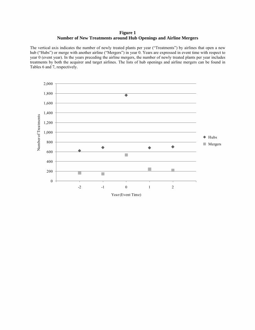
Figure 1 Number of New Treatments around Hub Openings and Airline Mergers

The vertical axis indicates the number of newly treated plants per year (“Treatments”) by airlines that open a new hub (“Hubs”) or merge with another airline (“Mergers”) in year 0. Years are expressed in event time with respect to year 0 (event year). In the years preceding the airline mergers, the number of newly treated plants per year includes treatments by both the acquirer and target airlines. The lists of hub openings and airline mergers can be found in Tables 6 and 7, respectively.

 

0

200

400

600

800

1,000

1,200

1,400

1,600

1,800

2,000

-3 -2 -1 0 1 2 3

Num

ber o

f Tre

atm

ents

Year (Event Time)

Hubs

Mergers

Table 1 Summary Statistics: Plants and Parent Companies

“All Plants” refers to all plants in the sample. “Eventually New Airline Route” refers to plants that are treated during the sample period, i.e., plants whose travel time to headquarters is reduced through the introduction of a new airline route. “No New Airline Route” refers to plants that are not treated during the sample period. Total Value of Ship-ments and Capital Stock are expressed in 1997 dollars (in 1,000s) using 4-digit SIC deflators from the NBER-CES Manufacturing Industry Database. Capital Stock is constructed using the perpetual inventory method described in Appendix B. Employees is the number of employees of the plant. Distance to Headquarters is the great-circle dis-tance between the plant’s ZIP code and the ZIP code of headquarters (in miles). Travel Time is the total travel time based on the fastest route and means of transportation (car or plane) between the plant’s ZIP code and the ZIP code of headquarters (in minutes). Employees (firm-level) and Number of Plants (firm-level) are the total number of em-ployees and the number of manufacturing plants, respectively, of the parent company to which the plant belongs. All figures are sample means. For plant-level (firm-level) variables, sample means are computed across all plant-year (firm-year) observations. Standard deviations are in parentheses. The sample period is from 1977 to 2005.

Eventually New No NewAll Plants Airline Route Airline Route

[1] [2] [3]

Total Value of Shipments 50,196 75,752 48,721(360,930) (222,685) (367,270)

Capital Stock 20,710 33,615 19,965(106,473) (118,024) (105,719)

Employees 213 300 208(568) (638) (564)

Distance to Headquarters (miles) 312 854 281(563) (616) (544)

Travel Time (minutes) 126 362 113(170) (135) (162)

Employees (firm-level) 591 5501 405(4,699) (16,136) (3,482)

Number of Plants (firm-level) 2.38 15.73 1.88(7.75) (24.40) (5.73)

Number of Observations 1,291,280 70,467 1,220,813

Table 2 Summary Statistics: Travel Time Reductions

“All” refers to all treated plants, i.e., plants whose travel time to headquarters is reduced through the introduction of a new airline route during the sample period. “Indirect to Indirect” refers to the subset of treated plants for which a new indirect flight using a different route replaces a previously optimal indirect flight. “Indirect to Direct” refers to the subset of treated plants for which a new direct flight replaces a previously optimal indirect flight. “Direct to Di-rect” refers to the subset of treated plants for which a new direct flight using a different route replaces a previously optimal direct flight. “Road to Flight” refers to the subset of treated plants for which a new direct or indirect flight replaces car travel as the previously optimal means of transportation. Distance to Headquarters is the great-circle distance between the plant’s ZIP code and the ZIP code of headquarters (in miles). Travel Time Before is the total travel time between the plant’s ZIP code and the ZIP code of headquarters based on the fastest route and means of transportation (car or plane) before the introduction of the new airline route (in minutes). Travel Time After is de-fined accordingly. Δ Travel Time is the difference between Travel Time After and Travel Time Before, expressed either in minutes or as a percentage of Travel Time Before. All figures are sample means across all plants. The sam-ple period is from 1977 to 2005.

Indirect to Indirect to Direct to Road toAll Indirect Direct Direct Flight

[1] [2] [3] [4] [5]

Distance to Headquarters (miles) 854 1,211 942 726 191

Travel Time Before (minutes) 417 566 466 338 253

Travel Time After (minutes) 314 420 339 266 206

∆ Travel Time (minutes) -103 -146 -127 -72 -47

∆ Travel Time (%) -25% -26% -27% -21% -19%

Number of Observations 10,533 1,911 3,469 4,544 609

Table 3 The Effect of New Airline Routes on Plant Investment and Productivity

Investment is the ratio of capital expenditures to capital stock, which is industry-adjusted by subtracting the industry median across all plants in a given 3-digit SIC industry and year. Total Factor Productivity (TFP) is the residual from estimating a log-linear Cobb-Douglas production function by Ordinary Least Squares for each 3-digit SIC in-dustry and year at the plant level. Treatment is a dummy variable that equals one if a new airline route that reduces the travel time between a plant and its headquarters has been introduced. MSA-year and Firm-year indicate the mean of the dependent variable in the plant’s MSA and firm, respectively, excluding the plant itself. Age is the natural logarithm of one plus the number of years since the plant has been in the LBD. Size is the natural logarithm of the number of employees of the plant. Standard errors are clustered at the MSA level. The sample period is from 1977 to 2005. Standard errors are in parentheses. *, **, and *** denotes significance at the 10%, 5%, and 1% level, re-spectively.

Dependent Variable:

[1] [2] [3] [4] [5] [6]

Treatment 0.008*** 0.009*** 0.010*** 0.014*** 0.013*** 0.013***(0.001) (0.001) (0.001) (0.003) (0.003) (0.003)

MSA-year 0.153*** 0.148*** 0.080*** 0.080***(0.022) (0.022) (0.012) (0.012)

Firm-year 0.205*** 0.205*** 0.186*** 0.186***(0.006) (0.006) (0.005) (0.005)

Age -0.060*** -0.061*** 0.015*** 0.018***(0.002) (0.002) (0.002) (0.003)

Size 0.029*** 0.012***(0.001) (0.002)

Plant Fixed Effects Yes Yes Yes Yes Yes YesYear Fixed Effects Yes Yes Yes Yes Yes YesSize × Year Fixed Effects No No Yes No No Yes

R-squared 0.39 0.41 0.41 0.60 0.61 0.61Number of Observations 1,291,280 1,291,280 1,291,280 1,291,280 1,291,280 1,291,280

Investment TFP

Table 4 Dynamic Effects of New Airline Routes

Treatment (-12m, -6m) is a dummy variable that equals one if the plant-year observation is recorded between six and 12 months before the introduction of the new airline route. Treatment (-6m, 0m), Treatment (0m, 6m), Treatment (6m, 12m), Treatment (12m, 18m), Treatment (18m, 24m), Treatment (24m, 30m), and Treatment (30m +) are de-fined analogously. All other variables are defined in Table 3. Standard errors are clustered at the MSA level. The sample period is from 1977 to 2005. Standard errors are in parentheses. *, **, and *** denotes significance at the 10%, 5%, and 1% level, respectively.

Dependent Variable: Investment TFP

[1] [2]

Treatment (-12m, -6m) -0.000 -0.001(0.003) (0.005)

Treatment (-6m, 0m) -0.001 -0.001(0.002) (0.004)

Treatment (0m, 6m) 0.003 0.001(0.003) (0.005)

Treatment (6m, 12m) 0.005** 0.006(0.002) (0.005)

Treatment (12m, 18m) 0.013*** 0.012**(0.003) (0.005)

Treatment (18m, 24m) 0.014*** 0.020***(0.002) (0.004)

Treatment (24m, 30m) 0.014*** 0.020***(0.003) (0.005)

Treatment (30m +) 0.009*** 0.013***(0.002) (0.004)

MSA-year 0.153*** 0.080***(0.022) (0.012)

Firm-year 0.205*** 0.186***(0.006) (0.005)

Age -0.060*** 0.015***(0.002) (0.002)

Size 0.029*** 0.012***(0.001) (0.002)

Plant Fixed Effects Yes YesYear Fixed Effects Yes Yes

R-squared 0.41 0.61Number of Observations 1,291,280 1,291,280

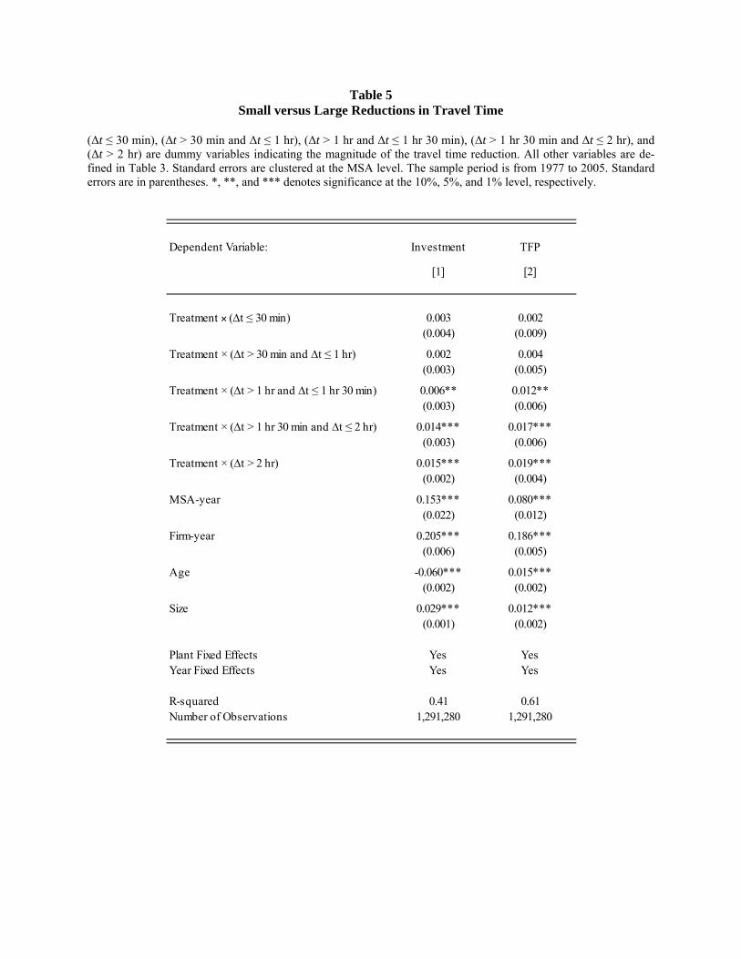
Table 5 Small versus Large Reductions in Travel Time

(Δt ≤ 30 min), (Δt > 30 min and Δt ≤ 1 hr), (Δt > 1 hr and Δt ≤ 1 hr 30 min), (Δt > 1 hr 30 min and Δt ≤ 2 hr), and (Δt > 2 hr) are dummy variables indicating the magnitude of the travel time reduction. All other variables are de-fined in Table 3. Standard errors are clustered at the MSA level. The sample period is from 1977 to 2005. Standard errors are in parentheses. *, **, and *** denotes significance at the 10%, 5%, and 1% level, respectively.

Dependent Variable: Investment TFP

[1] [2]

Treatment × (∆t ≤ 30 min) 0.003 0.002(0.004) (0.009)

Treatment × (∆t > 30 min and ∆t ≤ 1 hr) 0.002 0.004(0.003) (0.005)

Treatment × (∆t > 1 hr and ∆t ≤ 1 hr 30 min) 0.006** 0.012**(0.003) (0.006)

Treatment × (∆t > 1 hr 30 min and ∆t ≤ 2 hr) 0.014*** 0.017***(0.003) (0.006)

Treatment × (∆t > 2 hr) 0.015*** 0.019***(0.002) (0.004)

MSA-year 0.153*** 0.080***(0.022) (0.012)

Firm-year 0.205*** 0.186***(0.006) (0.005)

Age -0.060*** 0.015***(0.002) (0.002)

Size 0.029*** 0.012***(0.001) (0.002)

Plant Fixed Effects Yes YesYear Fixed Effects Yes Yes

R-squared 0.41 0.61Number of Observations 1,291,280 1,291,280

Table 6 Summary Statistics: Hub Openings

The table provides a list of airline hubs that are opened during the sample period. “Airline” is the name of the airline carrier. “City” is the city of the airport in which the new hub is opened (Federal Aviation Administration (FAA) 3-letter airport codes are in parentheses). “Year” is the year of the hub opening. The list is compiled from newspaper reports and airlines’ annual reports. The sample period is from 1977 to 2005.

Airline City Year

American Airlines Dallas (DFW) 1981

Piedmont Airlines Charlotte (CLT) 1981

American Airlines Chicago (ORD) 1982

Piedmont Airlines Dayton (DAY) 1982

Trans World Airlines St. Louis (STL) 1982

Western Airlines Salt Lake City (SLC) 1982

Piedmont Airlines Baltimore (BWI) 1983

Republic Airlines Detroit (DTW) 1984

Republic Airlines Memphis (MEM) 1985

America West Airlines Las Vegas (LAS) 1986

American Airlines Nashville (BNA) 1986

Eastern Airlines Philadelphia (PHL) 1986

Northwest Airlines Detroit (DTW) 1986

Northwest Airlines Memphis (MEM) 1986

Northwest Airlines Minneapolis (MSP) 1986

Piedmont Airlines Syracuse (SYR) 1986

United Airlines Washington (IAD) 1986

American Airlines Raleigh-Durham (RDU) 1987

Continental Airlines Cleveland (CLE) 1987

Delta Airlines Salt Lake City (SLC) 1987

American Airlines San Jose (SJC) 1988

Braniff Kansas City (MCI) 1988

American Airlines Miami (MIA) 1989

Delta Airlines Orlando (MCO) 1989

US Airways Baltimore (BWI) 1989

US Airways Charlotte (CLT) 1989

America West Airlines Columbus (CMH) 1991

Trans World Airlines Atlanta (ATL) 1992

United Airlines Los Angeles (LAX) 1997

Midwest Airlines Kansas City (MCI) 2000

Table 7 Summary Statistics: Airline Mergers

The table provides a list of airline mergers that are completed during the sample period and that account for at least one treatment during the sample period. The list includes only mergers that result in a merger of the airlines’ opera-tions. “Acquirer Airline” is the name of the acquiring airline carrier. “Target Airline” is the name of the acquired airline carrier. “Year” is the year in which the operations of the two airlines are merged. This list is compiled from newspaper reports, airlines’ annual reports, and the Securities Data Corporation (SDC) database. The sample period is from 1977 to 2005.

Acquirer Airline Target Airline Year

North Central Airlines Southern Airways 1979

Pan American World Airways National Airlines 1980

Republic Airlines Hughes Airwest 1980

Continental Airlines Texas International Airlines 1982

People Express Airlines Frontier Airlines 1985

Alaska Airlines Jet America Airlines 1986

American Airlines Air California 1986

Northwest Airlines Republic Airlines 1986

Piedmont Airlines Empire Airlines 1986

Trans World Airlines Ozark Airlines 1986

Continental Airlines New York Air 1987

Continental Airlines People Express Airlines 1987

Delta Airlines Western Airlines 1987

Braniff Florida Express 1988

US Airways Pacific Southwest Airlines 1988

US Airways Piedmont Airlines 1989

Air Wisconsin Aspen Airways 1990

Delta Airlines Pan American World Airways 1991

Southwest Airlines Morris Air 1994

AirTran Airways ValueJet Airlines 1997

American Airlines Reno Air 1999

American Airlines Trans World Airlines 2001

Table 8 Hub Openings and Airline Mergers

Treatment (Hub) and Treatment (Merger) are dummy variables that equal one if the treatment dummy equals one and the new airline route is introduced by an airline in the same year as it opens a new hub or merges its operations with another airline, respectively. Treatment (Other) is a dummy variable that equals one if the treatment dummy equals one and the treatment is not a hub or merger treatment as defined above. All other variables are defined in Table 3. Standard errors are clustered at the MSA level. The sample period is from 1977 to 2005. Standard errors are in parentheses. *, **, and *** denotes significance at the 10%, 5%, and 1% level, respectively.

Dependent Variable: Investment TFP

[1] [2]

Treatment (Hub) 0.017*** 0.019***(0.002) (0.005)

Treatment (Merger) 0.014** 0.018**(0.006) (0.009)

Treatment (Other) 0.008*** 0.011***(0.001) (0.003)

MSA-year 0.153*** 0.080***(0.022) (0.012)

Firm-year 0.205*** 0.186***(0.006) (0.005)

Age -0.060*** 0.015***(0.002) (0.002)

Size 0.029*** 0.012***(0.001) (0.002)

Plant Fixed Effects Yes YesYear Fixed Effects Yes Yes

R-squared 0.41 0.61Number of Observations 1,291,280 1,291,280

Table 9 New Airline Routes with Same Last Leg or Same First Leg

Treatment (Same Last Leg) and Treatment (Same First Leg) are dummy variables that equal one if the treatment dummy equals one and the new airline route operates the same last leg or the same first leg, respectively, as the pre-viously optimal airline route. Treatment (Other) is a dummy variable that equals one if the treatment dummy equals one and the new airline route operates neither the same last leg nor the same first leg as the previously optimal air-line route. All other variables are defined in Table 3. Standard errors are clustered at the MSA level. The sample period is from 1977 to 2005. Standard errors are in parentheses. *, **, and *** denotes significance at the 10%, 5%, and 1% level, respectively.

  

Dependent Variable: Investment TFP

[1] [2]

Treatment (Same Last Leg) 0.012*** 0.014*(0.004) (0.008)

Treatment (Same First Leg) 0.013*** 0.015**(0.004) (0.008)

Treatment (Other) 0.009*** 0.012***(0.001) (0.003)

MSA-year 0.153*** 0.080***(0.022) (0.012)

Firm-year 0.205*** 0.186***(0.006) (0.005)

Age -0.060*** 0.015***(0.002) (0.002)

Size 0.029*** 0.012***(0.001) (0.002)

Plant Fixed Effects Yes YesYear Fixed Effects Yes Yes

R-squared 0.41 0.61Number of Observations 1,291,280 1,291,280

Table 10 Alternative Control Groups

In columns [1] and [2], the sample is restricted to plants that belong to multi-unit firms consisting of more than one estab-lishment. In columns [3] and [4], the sample is restricted to plants that are eventually treated—i.e., plants whose travel time to headquarters is reduced through the introduction of a new airline route—during the sample period. Increase in Travel Time is a dummy variable that equals one if the travel time to headquarters increases during the sample period due to the termina-tion of an existing airline route. All other variables are defined in Table 3. Standard errors are clustered at the MSA level. The sample period is from 1977 to 2005. Standard errors are in parentheses. *, **, and *** denotes significance at the 10%, 5%, and 1% level, respectively.

Dependent Variable: Investment TFP Investment TFP Investment TFP

[1] [2] [3] [4] [5] [6]

Treatment 0.009*** 0.012*** 0.011*** 0.010*** 0.009*** 0.013***(0.001) (0.003) (0.002) (0.003) (0.001) (0.003)

Increase in Travel Time -0.005** -0.008*(0.002) (0.005)

MSA-year 0.133*** 0.090*** 0.084** 0.084** 0.153*** 0.083***(0.019) (0.015) (0.042) (0.041) (0.022) (0.012)

Firm-year 0.207*** 0.186*** 0.257*** 0.293*** 0.205*** 0.185***(0.006) (0.005) (0.016) (0.016) (0.006) (0.005)

Age -0.072*** 0.013*** -0.047*** 0.038*** -0.060*** 0.015***(0.002) (0.003) (0.004) (0.009) (0.002) (0.002)

Size 0.026*** 0.020*** 0.027*** 0.025*** 0.029*** 0.012***(0.001) (0.002) (0.002) (0.006) (0.001) (0.002)

Plant Fixed Effects Yes Yes Yes Yes Yes YesYear Fixed Effects Yes Yes Yes Yes Yes Yes

R-squared 0.37 0.61 0.32 0.65 0.41 0.61Number of Observations 825,097 825,097 70,467 70,467 1,282,228 1,282,228

Multi-unit Firms Increase in Travel TimeEventually Treated Plants

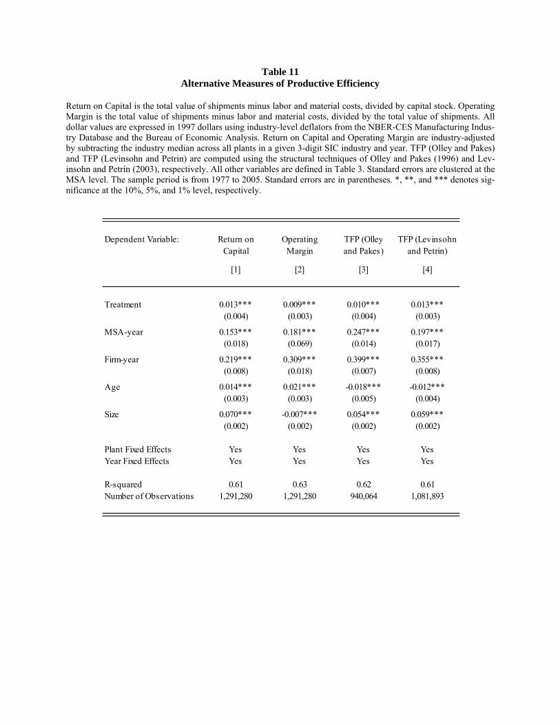
Table 11 Alternative Measures of Productive Efficiency

Return on Capital is the total value of shipments minus labor and material costs, divided by capital stock. Operating Margin is the total value of shipments minus labor and material costs, divided by the total value of shipments. All dollar values are expressed in 1997 dollars using industry-level deflators from the NBER-CES Manufacturing Indus-try Database and the Bureau of Economic Analysis. Return on Capital and Operating Margin are industry-adjusted by subtracting the industry median across all plants in a given 3-digit SIC industry and year. TFP (Olley and Pakes) and TFP (Levinsohn and Petrin) are computed using the structural techniques of Olley and Pakes (1996) and Lev-insohn and Petrin (2003), respectively. All other variables are defined in Table 3. Standard errors are clustered at the MSA level. The sample period is from 1977 to 2005. Standard errors are in parentheses. *, **, and *** denotes sig-nificance at the 10%, 5%, and 1% level, respectively.

Dependent Variable: Return on Operating TFP (Olley TFP (LevinsohnCapital Margin and Pakes) and Petrin)

[1] [2] [3] [4]

Treatment 0.013*** 0.009*** 0.010*** 0.013***(0.004) (0.003) (0.004) (0.003)

MSA-year 0.153*** 0.181*** 0.247*** 0.197***(0.018) (0.069) (0.014) (0.017)

Firm-year 0.219*** 0.309*** 0.399*** 0.355***(0.008) (0.018) (0.007) (0.008)

Age 0.014*** 0.021*** -0.018*** -0.012***(0.003) (0.003) (0.005) (0.004)

Size 0.070*** -0.007*** 0.054*** 0.059***(0.002) (0.002) (0.002) (0.002)

Plant Fixed Effects Yes Yes Yes YesYear Fixed Effects Yes Yes Yes Yes

R-squared 0.61 0.63 0.62 0.61Number of Observations 1,291,280 1,291,280 940,064 1,081,893

Table 12 Headquarters’ Time Constraints

In columns [1] and [2], headquarters’ time constraints are measured as the number of (white-collar) employees at headquarters divided by the total number of plants of the company (“Managers/Plants”). In columns [3] and [4], headquarters’ time constraints are measured as the number of (white-collar) employees at headquarters divided by the total distance (in miles) between headquarters and all of the company’s plants (“Managers/Total Distance”). High Time Constraints is a dummy variable that equals one if the measure of headquarters’ time constraint lies above the median value across all treated plants in the year prior to the treatment. Low Time Constraints is defined analogously. All other variables are defined in Table 3. Standard errors are clustered at the MSA level. The sample period is from 1977 to 2005. Standard errors are in parentheses. *, **, and *** denotes significance at the 10%, 5%, and 1% level, respectively.

Dependent Variable: Investment TFP Investment TFP

[1] [2] [3] [4]

Treatment × High Time Constraints 0.012*** 0.015*** 0.013*** 0.015***(0.002) (0.004) (0.002) (0.003)

Treatment × Low Time Constraints 0.006*** 0.010** 0.005** 0.009*(0.002) (0.004) (0.002) (0.005)

MSA-year 0.153*** 0.080*** 0.153*** 0.080***(0.022) (0.012) (0.022) (0.012)

Firm-year 0.205*** 0.186*** 0.205*** 0.186***(0.006) (0.005) (0.006) (0.005)

Age -0.060*** 0.015*** -0.060*** 0.015***(0.002) (0.002) (0.002) (0.002)

Size 0.029*** 0.012*** 0.029*** 0.012***(0.001) (0.002) (0.001) (0.002)

Plant Fixed Effects Yes Yes Yes YesYear Fixed Effects Yes Yes Yes Yes

R-squared 0.41 0.61 0.41 0.61Number of Observations 1,291,280 1,291,280 1,291,280 1,291,280

Managers/Plants Managers/Total Distance

Table 13 Innovations in Information Technology

Pre 1986, Between 1986 and 1995, and Post 1995 are dummy variables that equal one if the plant-year observation lies within the specified time interval. All other variables are defined in Table 3. Standard errors are clustered at the MSA level. The sample period is from 1977 to 2005. Standard errors are in parentheses. *, **, and *** denotes sig-nificance at the 10%, 5%, and 1% level, respectively.

Dependent Variable: Investment TFP

[1] [2]

Treatment × Pre 1986 0.013*** 0.019***(0.002) (0.004)

Treatment × Between 1986 and 1995 0.010*** 0.012***(0.002) (0.004)

Treatment × Post 1995 0.005** 0.009*(0.002) (0.005)

MSA-year 0.153*** 0.080***(0.022) (0.012)

Firm-year 0.205*** 0.186***(0.006) (0.005)

Age -0.060*** 0.015***(0.002) (0.002)

Size 0.029*** 0.012***(0.001) (0.002)

Plant Fixed Effects Yes YesYear Fixed Effects Yes Yes

R-squared 0.41 0.61Number of Observations 1,291,280 1,291,280