PSMA Magnetics Committee

Core Loss, Phase III

Final Report1

John H.Harris

20 March 2013

1Revision 310

Contents

1 Introduction 1

2 Parasitic Loss Experiment 12.1 Experimental Setup . . . . . . . . . . . . . . . . . . . . . . . . . 22.2 Reproducibility . . . . . . . . . . . . . . . . . . . . . . . . . . . . 3

2.2.1 Chaotic Waveform Transients . . . . . . . . . . . . . . . . 52.2.2 Marginal Gate Drive Voltage . . . . . . . . . . . . . . . . 52.2.3 Power Supply Wiring . . . . . . . . . . . . . . . . . . . . 7

3 Winding Variations 73.1 The Hairpin Core . . . . . . . . . . . . . . . . . . . . . . . . . . . 83.2 Hairpin Core Performance . . . . . . . . . . . . . . . . . . . . . . 83.3 Effect on Dead-time Loss Behavior . . . . . . . . . . . . . . . . . 11

4 Independent Testing 14

5 Data Availability 14

List of Tables

1 Cores used in the experiments . . . . . . . . . . . . . . . . . . . . 32 Runs sets added in Phase III . . . . . . . . . . . . . . . . . . . . 14

List of Figures

1 Drive bridge schematic detail . . . . . . . . . . . . . . . . . . . . 22 Deviation of baseline set losses . . . . . . . . . . . . . . . . . . . 43 Deviation of parasitic loss runs . . . . . . . . . . . . . . . . . . . 44 Routine test waveform . . . . . . . . . . . . . . . . . . . . . . . . 65 Lossy bridge waveform . . . . . . . . . . . . . . . . . . . . . . . . 66 The hairpin test device . . . . . . . . . . . . . . . . . . . . . . . . 87 Cross-section of the hairpin test device . . . . . . . . . . . . . . . 88 Hairpin core loss deviation vs. loss . . . . . . . . . . . . . . . . . 99 Hairpin core loss deviation vs. V· s . . . . . . . . . . . . . . . . . 910 Hairpin core loss (3-D) . . . . . . . . . . . . . . . . . . . . . . . . 1011 Comparison of hairpin and toroidal core oscilloscope plots . . . . 1212 Comparison of hairpin and toroidal core oscilloscope plots . . . . 1213 Expand waveform losses with the toroidal core . . . . . . . . . . 1314 Expand waveform losses with the hairpin core . . . . . . . . . . . 13

1 Introduction

Phase III of PSMA Magnetics Committee Core Loss Project is a collection ofsmall, exploratory subprojects. The project statement of work (SOW) lists fivesubprojects:

1. Test intentionally added parasitic impedances in the test equipment to seeif they affect the data, with one representative core.

2. Test some winding variations in simulation and in practice, to see if theyaffect the data.

3. Additional testing with powder cores.

4. A series of tests with constant frequency and constant peak flux density(constant volt-seconds), but with varying on-time and voltage. These willbe conducted for three cores.

5. Swap cores with ETH [Jonas Muehlethaler at ETH, Zurich], and try toduplicate each others’ data.

6. Complete tests on the nanocrystaline core.

Of these, we were only able to conduct items 1, 2, and 5, with the availablebudget, primarily due to time spent on quality control tasks and consequen-tial troubleshooting. These included testing experiment reproducibility, andmeasures to control possible sources of variation in the data. The conductedsubprojects are discussed in the following sections

2 Parasitic Loss Experiment

From the project SOW:

1. Test intentionally added parasitic impedances in the test equipment to seeif they affect the data, with one representative core.

The utility of this experiment is subtle—our basic approach to measuring coreloss is immune to problems with the drive circuit because it measures the voltagedue to flux (with the sense winding) and current directly, giving us a shortinferential path to the instantaneous power and energy per cycle, but there arestill some possible error sources:

1. We are trying to measure the core loss given a particular voltage waveform:a clean, square, pulse-width-modulated (PWM) waveform. Poor fidelity inapplying that waveform could produce misleading results—the apparatuswill faithfully report the core loss of whatever waveform is applied—evenif it distorted.

2. There can be problems with the functioning and calibration of the testinstruments.

1

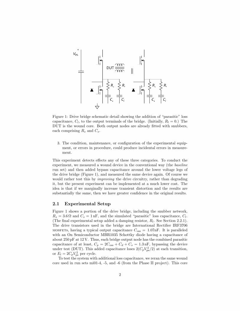
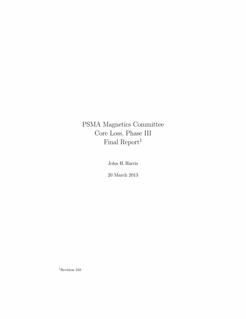
Figure 1: Drive bridge schematic detail showing the addition of “parasitic” losscapacitance, Cl, to the output terminals of the bridge. (Initially, Rl = 0.) TheDUT is the wound core. Both output nodes are already fitted with snubbers,each comprising Rs and Cs.

3. The condition, maintenance, or configuration of the experimental equip-ment, or errors in procedure, could produce incidental errors in measure-ment.

This experiment detects effects any of these three categories. To conduct theexperiment, we measured a wound device in the conventional way (the baselinerun set) and then added bypass capacitance around the lower voltage legs ofthe drive bridge (Figure 1), and measured the same device again. Of course wewould rather test this by improving the drive circuitry, rather than degradingit, but the present experiment can be implemented at a much lower cost. Theidea is that if we marginally increase transient distortion and the results aresubstantially the same, then we have greater confidence in the original results.

2.1 Experimental Setup

Figure 1 shows a portion of the drive bridge, including the snubber network,Rs = 3.6Ω and Cs = 1nF, and the simulated “parasitic” loss capacitance, Cl.(The final experimental setup added a damping resistor, Rl. See Section 2.2.1).The drive transistors used in the bridge are International Rectifier IRF3706mosfets, having a typical output capacitance Coss = 1.07nF. It is paralleledwith an On Semiconductor MBR1035 Schottky diode having a capacitance ofabout 250 pF at 12V. Thus, each bridge output node has the combined parasiticcapacitance of at least, Cp = 2Coss + Cd + Cs = 1.3 nF, bypassing the deviceunder test (DUT). This added capacitance loses 2(CpV

2ps/2) at each transition,

or El = 2CpV2ps per cycle.

To test the system with additional loss capacitance, we reran the same woundcore used in run sets mi01-4, -5, and -6 (from the Phase II project). This core

2

Shape Material Mfg lot Ae height do/di[mm2] [mm]

40402TC F S00809 3.1 2.54 2.1142206TC F PS0142 26.2 6.35 1.6142206TC P S00841 26.242206TC R n/a 26.2

Table 1: Cores used in the experiments in Phase III were all manufactured byMagnetics, Inc., who provided the data above.

is of Magnetics Inc. R material, in the 42206-TC shape (Table 1), wound with5 turns. In the present run sets, the bridge was switched at from 20 to 500 kHz.The power supply voltage ranged up to 12.5V. At that voltage, with Cl = 0,El is about 0.5µJ. Only the square waveforms were used.

The baseline run set (no added loss capacitors), was named mi01-7. To geta feeling for baseline parasitic capacitance loss, the highest measured core lossper cycle, Ecyc was 6.6µJ; the baseline parasitic capacitance loss (due to Cp) isless than 8% (or 0.3 dB) of this core loss.

A second set, mi01-8, was identical, but with the added loss capacitors havingCl = 1.0 nF (but Rl = 0). The added loss capacitance, Cl, is on the order ofCp, but from a casual comparison of the conventional loss plots it appeared thatthe addition of Cl caused little change in the measured core losses.

To push it further, a third set was run, mi01-9, with Cl = 4.7 nF—overthree times Cp, making the capacitive switching loss about 37% of the expectedcore loss. This gave us two incremental additions of loss that we could examinequantitatively. Around this point in the project, we began to notice problemswith reproducibility, which are discussed in more detail in Section 2.2.

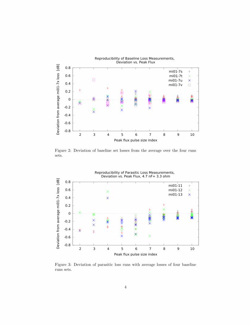
After modifying the apparatus for improved reproducibility, four baselinesets were run, mi01-7s, t, u, and v (Figure 2). Most of the baseline measurementswere consistent within about±0.2 dB. With the parasitic loss setup, we obtainedbetter waveform fidelity and reproducibility with the addition of Rl = 3.3Ω.Three sets were run with this modification, mi01-11, -12, and -13. Figure 3shows the deviation of the parasitic loss runs from the averages of the baselineruns. These sets tend to measure lower core loss, by about 0.2 dB, but thesignificance of this is difficult to assess with such a small sample. To keepthis in perspective, the standard error for the two-plane Steinmetz curve fit forrun mi01-7 was 0.4 dB (about ±9.3%), while we have increased the capacitiveswitching loss by 1.4 dB (37%). We conclude that this experiment gives noevidence that variations in the drive bridge switching losses have a significanteffect on our core loss measurements.

2.2 Reproducibility

This section is presented to aid in project management. The discussion is notquantitative, since the repair work was not the objective of the project, but

3

-0.8

-0.6

-0.4

-0.2

0

0.2

0.4

0.6

0.8

2 3 4 5 6 7 8 9 10Devia

tion f

rom

avera

ge m

i01

-7x loss

[dB

]

Peak flux pulse size index

Reproducibility of Baseline Loss Measurements, Deviation vs. Peak Flux

mi01-7s

mi01-7t

mi01-7u

mi01-7v

Figure 2: Deviation of baseline set losses from the average over the four runssets.

-0.8

-0.6

-0.4

-0.2

0

0.2

0.4

0.6

0.8

2 3 4 5 6 7 8 9 10Devia

tion f

rom

avera

ge m

i01-7

x loss [d

B]

Peak flux pulse size index

Reproducibility of Parasitic Loss Measurements, Deviation vs. Peak Flux, 4.7 nF+ 3.3 ohm

mi01-11

mi01-12

mi01-13

Figure 3: Deviation of parasitic loss runs with average losses of four baselineruns sets.

4

rather a hurdle that needed to be overcome to complete the investigation withconfidence in the measurements.

Initial runs comparing measurements with and without added parasitics gaveinconsistent results. Tracing the cause of these discrepancies accounts for mostof the effort in the parasitic loss subproject. Three important effects whereconsidered:

1. Chaotic waveform transients, caused by loss capacitance (Cl) ringing.

2. Marginal bridge mosfet gate drive voltage.

3. Microphonic power-lead connector resistance.

Of these, the first and third had the greatest effect, but they are presented inthe following sections in the order in which they were investigated.

2.2.1 Chaotic Waveform Transients

An initial test with Cl = 1nF had a conventional core loss plot that lookedqualitatively very similar to the baseline plot. To push it further, a third setwas run, mi01-9, with Cl = 4.7 nF—over three times Cp. This provided twoincremental additions of loss that could be examined quantitatively. Plottingboth the Cl = 1nF and 4.7 nF losses versus pulse width, showed a scattering ofpoints, suggesting some kind of problem.

Looking for clues for this apparent anomaly, it is useful to examine theoscilloscope plots. Figures 4 and 5 show plots for runs mi01-7-001 and mi01-9-001, both for pulse width t1 = 1µs (T = 2µs). The most striking difference isthe increased ringing, now at about 10MHz.

If high-frequency ringing initiated by one switching transition is not suffi-ciently damped to be present at the next switching transition, the exact phasingbetween the ringing and the switching event can have a significant effect, andsmall jitter in timing can greatly change this phase if the ringing is at sufficientlyhigh frequency.

To remedy this, a damping resistor was added, Rl = 3.3Ω, which signifi-cantly improved reproducibility.

2.2.2 Marginal Gate Drive Voltage

Looking for reproducibility problems suggested problems with hardware reli-ability. There had been some problems with gate drive power supply batterycontact resistance. The bridge circuit has four legs, two for connecting the DUTterminals to ground, and two for connecting device terminals to the power sup-ply positive terminal, the high side. The ground-side gate drives have alwaysbeen powered by the same 10V power supply that runs the decoder logic anddead-time circuitry. The high-side gate drives “float”—they are referenced tothe bridge output terminals, which range from 0 to 12.5V above ground. In theoriginal machine, (before August 2012) each high-side gate drive was poweredby a single, rechargeable, 8.4V Ni-MH battery.

5

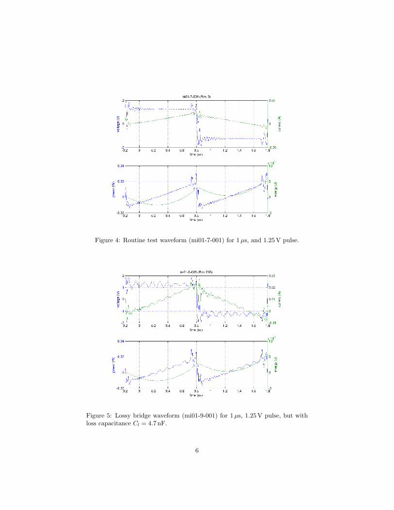
Figure 4: Routine test waveform (mi01-7-001) for 1µs, and 1.25V pulse.

Figure 5: Lossy bridge waveform (mi01-9-001) for 1µs, 1.25V pulse, but withloss capacitance Cl = 4.7 nF.

6

That design could be vulnerable to battery charge-state variations, thoughit was not clear whether it was contributing to the observed reproducibilityproblems. To eliminate that possibility and to avoid the need to perform time-consuming testing to verify the extent of its importance, we added voltage reg-ulators to the gate drive supplies.

To do this we added simple three-terminal regulators (Micrel Inc. MIC2940A),each referenced to its bridge output terminal. A second battery was added inseries on each side, doubling the input voltage, to provide ample headroom forregulation, down to 12V. After installing the new gate drive power supplies, thedead time timing was rechecked, and found to be satisfactory.

2.2.3 Power Supply Wiring

Some problems with reproducibility were traced to the wire leads between theprogrammable power supply and the bridge assembly. The wires were boltedto the power supply terminals, and fitted with banana plugs to connect to thebridge assembly. Both banana plugs were old, of low-quality manufacture, andhad fatigued, flattened contact leaves. They fit so loosely in the jacks that itwas impossible to measure a meaningful voltage drop across the connection.It may be that vibrations transmitted from the stirred oil coolant could haveintroduced microphonic noise into the applied drive voltage. These connectorswere replaced with new, high-quality banana plugs, resulting in much improvedreproducibility.

3 Winding Variations

From the project SOW:

2. Test some winding variations in simulation and in practice, to see if theyaffect the data.

We would like to see if a simpler flux geometry influences the “dead-time loss”phenomenon discovered in Phase I—losses for PWM waveforms having deadtime (i.e., periods of zero drive voltage and constant flux) are greater thanpredicted by the composite waveform hypothesis. Most of the cores tested inthis project in the past were toroidal, wound with about five turns in a simple,helical lay.

In this exploratory experiment we compare a typical five-turn toroidal-coredevice used in previous experiments, with an “equivalent,” single-turn, “hairpin”device (Figure 6). The intent is to have a non-helical winding geometry, so thatflux lines are oriented in the plane perpendicular to the wire. The hairpin core isnot ideal (most notably, the geometry does not guarantee that the flux density isidentical around the perimeter of the core, and it can be higher near return-pathstring of cores), but solves two problems:

1. With a single turn on our typical core geometry, the present apparatuscan not supply enough current for our range of flux densities. To use the

7

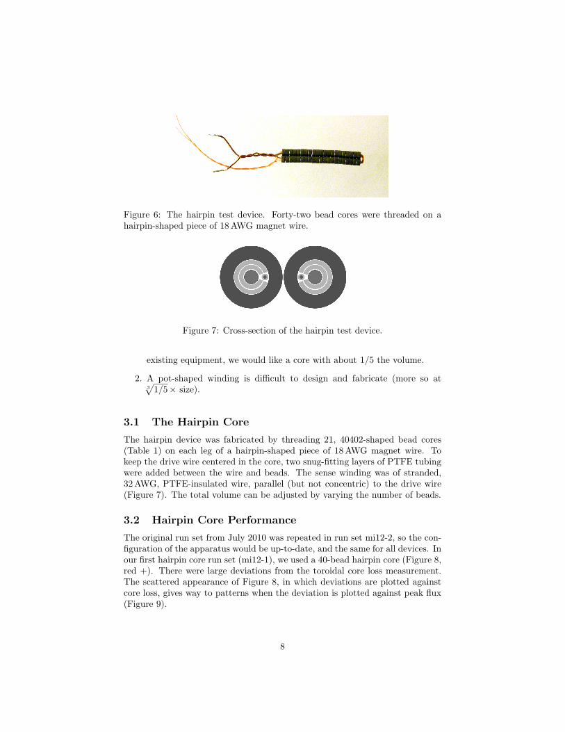
Figure 6: The hairpin test device. Forty-two bead cores were threaded on ahairpin-shaped piece of 18AWG magnet wire.

Figure 7: Cross-section of the hairpin test device.

existing equipment, we would like a core with about 1/5 the volume.

2. A pot-shaped winding is difficult to design and fabricate (more so at3√1/5× size).

3.1 The Hairpin Core

The hairpin device was fabricated by threading 21, 40402-shaped bead cores(Table 1) on each leg of a hairpin-shaped piece of 18AWG magnet wire. Tokeep the drive wire centered in the core, two snug-fitting layers of PTFE tubingwere added between the wire and beads. The sense winding was of stranded,32AWG, PTFE-insulated wire, parallel (but not concentric) to the drive wire(Figure 7). The total volume can be adjusted by varying the number of beads.

3.2 Hairpin Core Performance

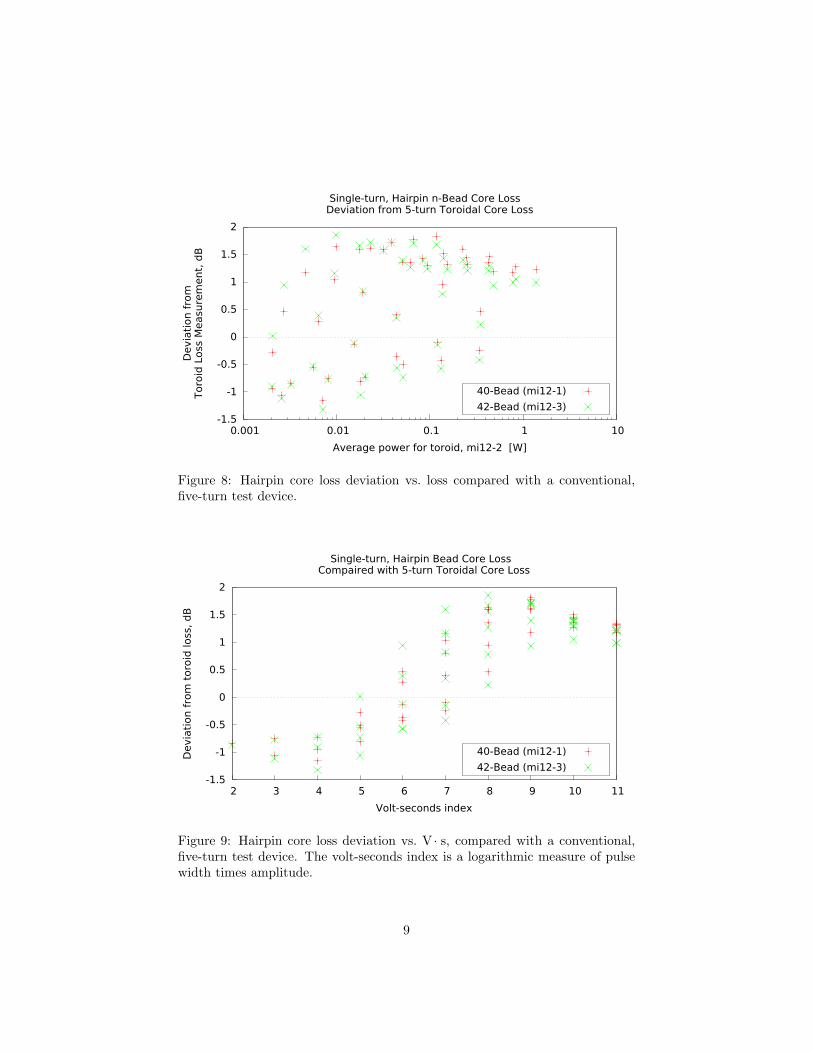
The original run set from July 2010 was repeated in run set mi12-2, so the con-figuration of the apparatus would be up-to-date, and the same for all devices. Inour first hairpin core run set (mi12-1), we used a 40-bead hairpin core (Figure 8,red +). There were large deviations from the toroidal core loss measurement.The scattered appearance of Figure 8, in which deviations are plotted againstcore loss, gives way to patterns when the deviation is plotted against peak flux(Figure 9).

8

-1.5

-1

-0.5

0

0.5

1

1.5

2

0.001 0.01 0.1 1 10

Devia

tion f

rom

Toro

id L

oss M

easure

ment,

dB

Average power for toroid, mi12-2 [W]

Single-turn, Hairpin n-Bead Core Loss Deviation from 5-turn Toroidal Core Loss

40-Bead (mi12-1)

42-Bead (mi12-3)

Figure 8: Hairpin core loss deviation vs. loss compared with a conventional,five-turn test device.

-1.5

-1

-0.5

0

0.5

1

1.5

2

2 3 4 5 6 7 8 9 10 11

Devia

tion f

rom

toro

id loss,

dB

Volt-seconds index

Single-turn, Hairpin Bead Core Loss Compaired with 5-turn Toroidal Core Loss

40-Bead (mi12-1)

42-Bead (mi12-3)

Figure 9: Hairpin core loss deviation vs. V · s, compared with a conventional,five-turn test device. The volt-seconds index is a logarithmic measure of pulsewidth times amplitude.

9

1 2

3 4

5 6

1 2

3 4

5 6

7 8

9 1

0-1

.5-1-0

.5 0 0

.5 1 1

.5 2

Deviation from toroid loss, dB

Devia

tion o

f H

air

pin

n-B

ead L

oss

Re:

5-t

urn

Toro

idal C

ore

Loss

40

-bead

42

-bead

V index

T index

Deviation from toroid loss, dB

Figure

10:Hairpin

core

loss

(3-D

)comparedwithaconvention

al,five-turn

test

device.

TheV

andT

indices

are

loga

rithmic

measuresof

pulsewidth

andam

plitude.

10

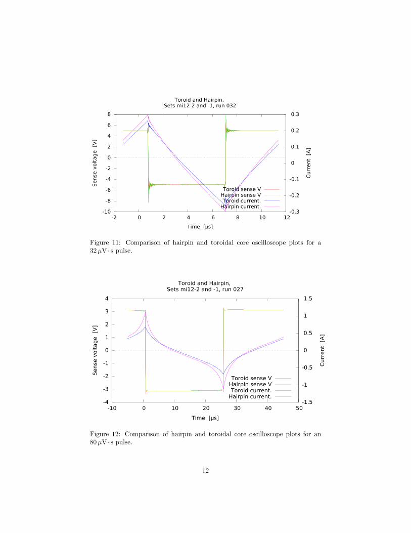
Comparing oscilloscope plots of for run 032 (32µV· s pulse) from both thehairpin and toroid core run sets (Figure 11) shows the sense voltages agree well,but the hairpin device has a lower inductance than the toroid; This would notaccount for the increased core loss, and suggests earlier saturation. This couldbe attributed to the different ratios of core inner to outer diameter, di/do, ofthe full-size and bead cores. The smaller di/do ratio of the bead core leads togreater flux crowding at the inside diameter, where saturation begins.

Comparing oscilloscope plots for run 027 confirms this (Figure 12). Run027 drives the core harder, with an 80µV· s pulse. Again the sense voltagesagree well, but the hairpin core has a much higher peak current, and a moreexaggerated rise in di/dt due to saturation.

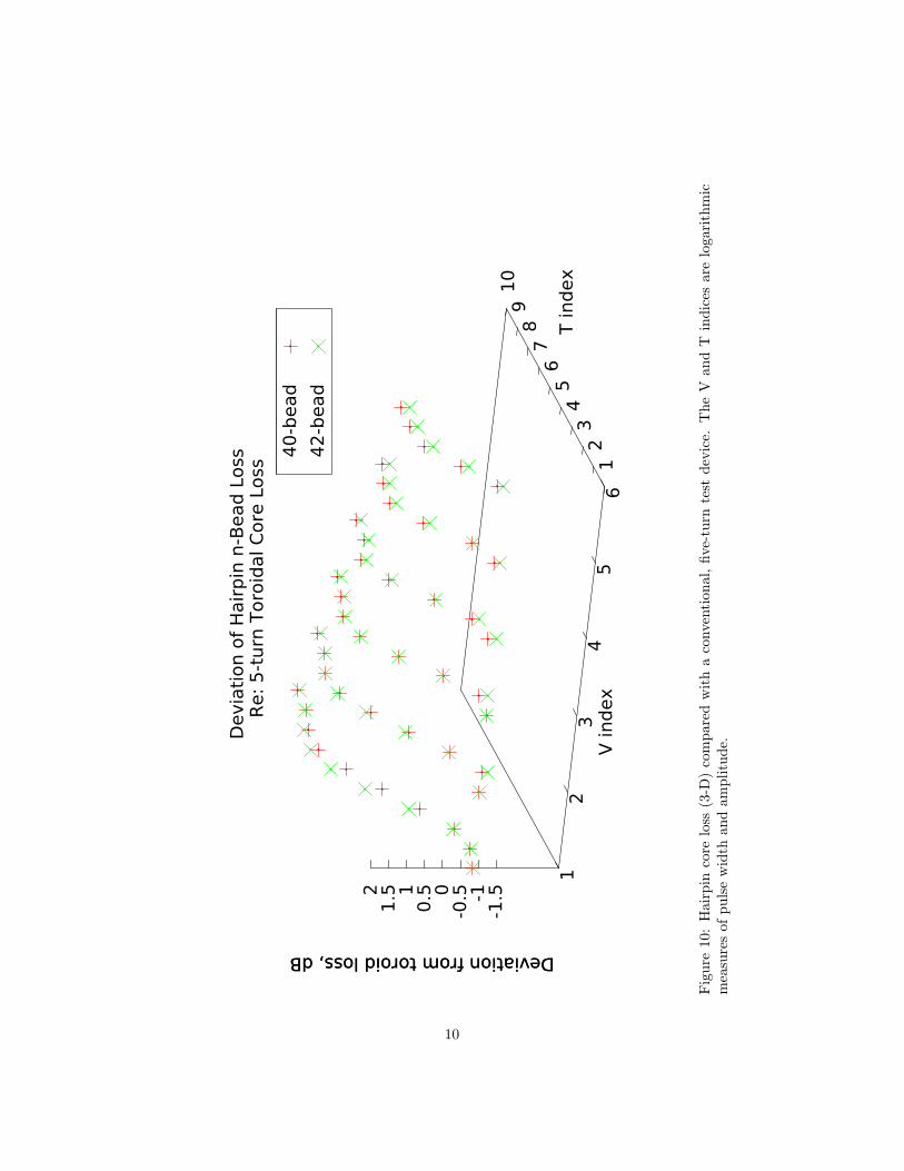
Two more beads were added to create a 42-core device with larger total corecross-section area for run set mi12-3. Figure 9 shows these results with greenxs. The results are similar to those with the 40-core device. Figure 10 separatesdrive pulse amplitude from width, adding another dimension. (The abscissa ofFigure 9, “volt-seconds index” is just the sum of Figure 10’s V and T indices.)

There are several effects that could account for the differences measured.More detailed modeling of these could help explain the differences.

• As noted above di/do is significantly lower for the hairpin cores, comparedto the toroidal core (Table 1), which means a higher radial flux gradientfor a given peak flux, resulting in an earlier onset of saturation. A one-dimensional (radial) analysis can account for this effect.

An alternative approach to examining this effect would be to eliminate itby custom fabricating cores in two sizes, but with identical di/do, prefer-ably from the same batch of material.

• With the onset of saturation, there is asymmetry in flux leakage, resultingin greater saturation in a localized region of the core where it is adjacentto the other core. A two-dimensional, finite-element analysis would berequired to model this.

3.3 Effect on Dead-time Loss Behavior

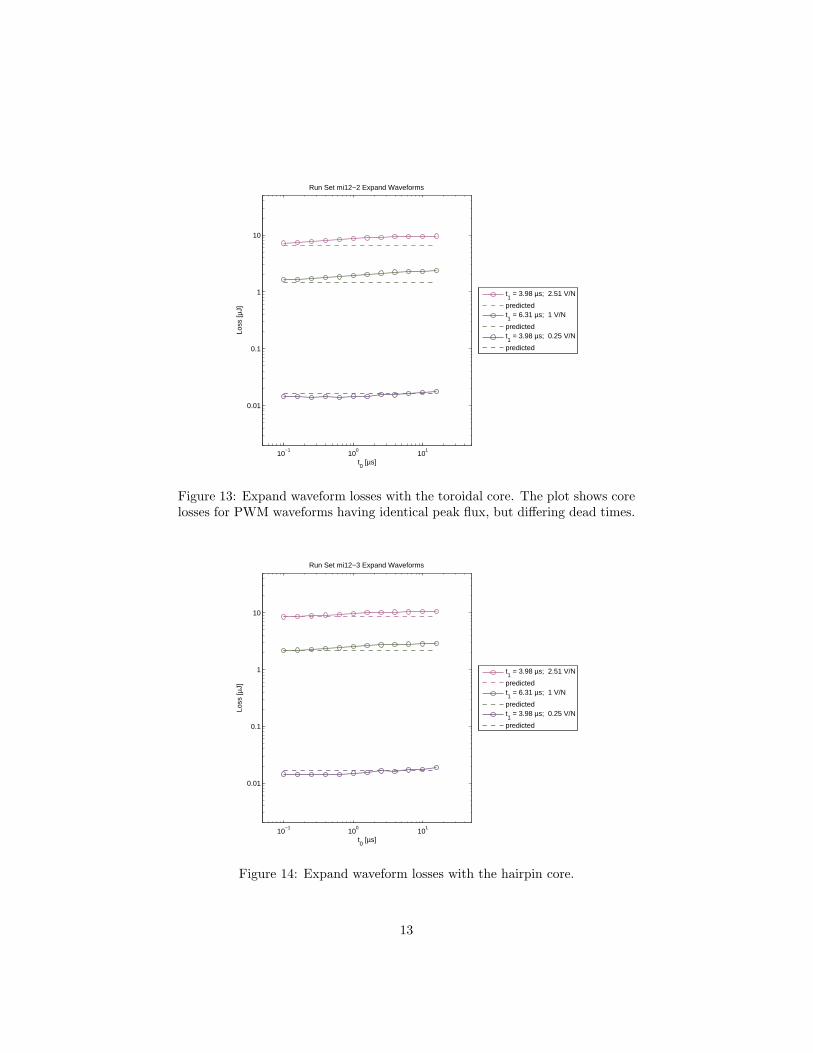
While the hairpin device we fabricated is not an exact simulation of the 42206core with a pot winding, it does capture the feature of interest—unlike a helically-wound toroidal device, the flux loops are predominately planar—and in parallelplanes, at that (unlike the pot-shaped winding). The most direct indicator ofthe dead-time loss phenomenon is the expand waveform series of runs. Figures13 and 14 show little qualitative difference between the toroidal and hairpincores with this series. The hairpin core has somewhat less overall increase inloss (1.1 dB versus 2.0 dB for 32µV· s pulses), but the overall shape of the curveis similar.

11

-10

-8

-6

-4

-2

0

2

4

6

8

-2 0 2 4 6 8 10 12-0.3

-0.2

-0.1

0

0.1

0.2

0.3

Sense v

olt

age

[V]

Curr

ent

[A

]

Time [µs]

Toroid and Hairpin, Sets mi12-2 and -1, run 032

Toroid sense VHairpin sense VToroid current.

Hairpin current.

Figure 11: Comparison of hairpin and toroidal core oscilloscope plots for a32µV· s pulse.

-4

-3

-2

-1

0

1

2

3

4

-10 0 10 20 30 40 50-1.5

-1

-0.5

0

0.5

1

1.5

Sense v

olt

age [V

]

Curr

ent

[A

]

Time [µs]

Toroid and Hairpin, Sets mi12-2 and -1, run 027

Toroid sense VHairpin sense VToroid current.

Hairpin current.

Figure 12: Comparison of hairpin and toroidal core oscilloscope plots for an80µV· s pulse.

12

10−1

100

101

0.01

0.1

1

10

t0 [µs]

Loss

[µJ]

Run Set mi12−2 Expand Waveforms

t1 = 3.98 µs; 2.51 V/N

predictedt1 = 6.31 µs; 1 V/N

predictedt1 = 3.98 µs; 0.25 V/N

predicted

Figure 13: Expand waveform losses with the toroidal core. The plot shows corelosses for PWM waveforms having identical peak flux, but differing dead times.

10−1

100

101

0.01

0.1

1

10

t0 [µs]

Loss

[µJ]

Run Set mi12−3 Expand Waveforms

t1 = 3.98 µs; 2.51 V/N

predictedt1 = 6.31 µs; 1 V/N

predictedt1 = 3.98 µs; 0.25 V/N

predicted

Figure 14: Expand waveform losses with the hairpin core.

13

4 Independent Testing

To get an independent check on the reproducibility of our results, we woundtwo devices to be measured first with our apparatus, and then shipped to JonasMuehlethaler at ETH, Zurich, for testing on their apparatus. Both cores werewound with 5 turns, on cores manufactured by Magnetics, Inc., in their 42206toroidal shape, one each from the F and P materials (Table 1, run sets mi05-6and mi03-2, respectively).

5 Data Availability

The data have been supplied if the same format as was used in Phase II, and willbe available at http://engineering.dartmouth.edu/inductor/psma/. Ta-ble 2 summarizes the run sets added in Phase III. Data gathered using theunimproved drive electronics was used only for diagnosis, and will not be posted.

SubprojectSet IDs Description

Parasitic loss comparison.mi01-7 Original baseline run set to be compared with loss

capacitor sets. This run set was not posted, havingbeen replaced by set mi01-7v.

mi01-7x Series of baseline run sets, x = s, t, u, v, us-ing the improved bridge electronics, to check forreproducibility.

mi01-8 The initial lossy-bridge run set, with Cl = 1nF,Rl = 0. Not posted.

mi01-9, -10 Cl = 4.7 nF, Rl = 0. Not posted.mi01-11, -12, -13 Series of lossy-bridge run sets with Cl = 4.7 nF,

Rl = 3.3Ω.Hairpin core.

mi12-1 Forty-bead hairpin core.mi12-2 Baseline 5-turn toroidal core.mi12-3 Forty-two-bead hairpin core.

Independent testing.mi03-2 0P42206 core with 5 turns.mi05-6 0F42206 core with 5 turns.

Table 2: Runs sets added in Phase III. Runs sets with the unimproved driveelectronics have not been posed on the data web page.

14