PT 4PRESSURE TRANSIENT ANALYSIS SOFTWARE

USER’S GUIDE

Copyright 1991-2007 The Comport Computing CompanyAll Rights Reserved

The Comport Computing Company12230 Palmfree St., Houston, Texas 77034, U. S. A.

(713) 947-3363www.comportco.com

Page 1

PT 4 Software

LICENSE AGREEMENT

This software is protected by United States copyright law and international treaty provisions. The ComPort Computing Company authorizes you to make archival copies of the software for the sole purpose of backing-up your software and protecting against software loss. You may move this software from computer to computer freely, as long as there is no possibility of the software being used by two different people at two locations at the same time. This software may not be copied for the purpose of sales or distribution without the express written consent of the ComPort Computing Company.

For technical support issues, please contact wfair@comportco.com.

LIMITED WARRANTY

The ComPort Computing Company warrants the diskette or other distribution medium to be free from defects in materials or workmanship for a period of 60 days from the date of purchase. In the event of such defect, the ComPort Computing Company will replace the defective medium. Contact the ComPort Computing Company for instructions and a return authorization.

The ComPort Computing Company shall not be liable for any damages arising from the use of this product. All other warranties, express or implied, are specifically disclaimed.

ACKNOWLEDGMENTSWindows, Windows NT, Windows 95, Windows ME, Windows 2000 and Windows XP are all registered trademarks of the Microsoft Corporation. Echometer is a registered trademark of the Echometer Company.

Page 2

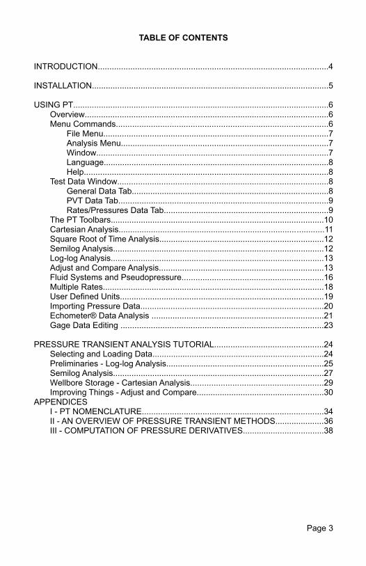
TABLE OF CONTENTS

INTRODUCTION...................................................................................................4

INSTALLATION......................................................................................................5

USING PT..............................................................................................................6Overview.........................................................................................................6Menu Commands...........................................................................................6

File Menu.................................................................................................7Analysis Menu.........................................................................................7Window....................................................................................................7Language.................................................................................................8Help.........................................................................................................8

Test Data Window...........................................................................................8General Data Tab.....................................................................................8PVT Data Tab..........................................................................................9Rates/Pressures Data Tab.......................................................................9

The PT Toolbars............................................................................................10Cartesian Analysis.........................................................................................11Square Root of Time Analysis.......................................................................12Semilog Analysis...........................................................................................12Log-log Analysis............................................................................................13Adjust and Compare Analysis.......................................................................13Fluid Systems and Pseudopressure.............................................................16Multiple Rates...............................................................................................18User Defined Units........................................................................................19Importing Pressure Data...............................................................................20Echometer® Data Analysis ..........................................................................21Gage Data Editing .......................................................................................23

PRESSURE TRANSIENT ANALYSIS TUTORIAL...............................................24Selecting and Loading Data..........................................................................24Preliminaries - Log-log Analysis....................................................................25Semilog Analysis...........................................................................................27Wellbore Storage - Cartesian Analysis.........................................................29Improving Things - Adjust and Compare.......................................................30

APPENDICESI - PT NOMENCLATURE..............................................................................34II - AN OVERVIEW OF PRESSURE TRANSIENT METHODS.....................36III - COMPUTATION OF PRESSURE DERIVATIVES...................................38

Page 3

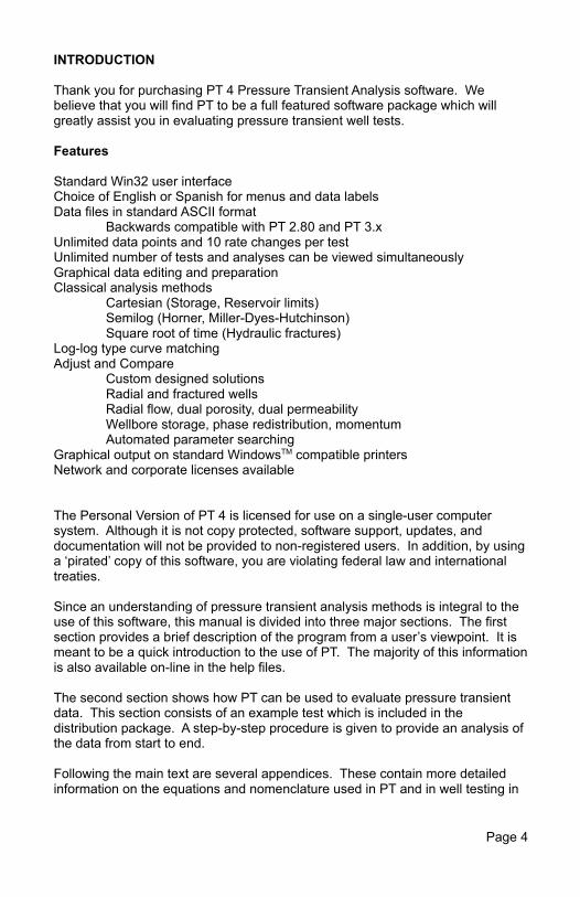
INTRODUCTION

Thank you for purchasing PT 4 Pressure Transient Analysis software. We believe that you will find PT to be a full featured software package which will greatly assist you in evaluating pressure transient well tests.

Features

Standard Win32 user interfaceChoice of English or Spanish for menus and data labelsData files in standard ASCII format

Backwards compatible with PT 2.80 and PT 3.xUnlimited data points and 10 rate changes per testUnlimited number of tests and analyses can be viewed simultaneouslyGraphical data editing and preparationClassical analysis methods

Cartesian (Storage, Reservoir limits)Semilog (Horner, Miller-Dyes-Hutchinson)Square root of time (Hydraulic fractures)

Log-log type curve matchingAdjust and Compare

Custom designed solutionsRadial and fractured wellsRadial flow, dual porosity, dual permeabilityWellbore storage, phase redistribution, momentumAutomated parameter searching

Graphical output on standard WindowsTM compatible printersNetwork and corporate licenses available

The Personal Version of PT 4 is licensed for use on a single-user computer system. Although it is not copy protected, software support, updates, and documentation will not be provided to non-registered users. In addition, by using a ‘pirated’ copy of this software, you are violating federal law and international treaties.

Since an understanding of pressure transient analysis methods is integral to the use of this software, this manual is divided into three major sections. The first section provides a brief description of the program from a user’s viewpoint. It is meant to be a quick introduction to the use of PT. The majority of this information is also available on-line in the help files.

The second section shows how PT can be used to evaluate pressure transient data. This section consists of an example test which is included in the distribution package. A step-by-step procedure is given to provide an analysis of the data from start to end.

Following the main text are several appendices. These contain more detailed information on the equations and nomenclature used in PT and in well testing in

Page 4

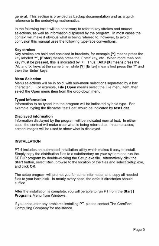
general. This section is provided as backup documentation and as a quick reference to the underlying mathematics.

In the following text it will be necessary to refer to key strokes and mouse selections, as well as information displayed by the program. In most cases the context will make it obvious what is being referred to, however, to avoid confusion this manual uses the following type-face conventions:

Key strokesKey strokes are bold and enclosed in brackets, for example [Y] means press the key labeled ‘Y’, [Enter] means press the ‘Enter’ key, etc. When more than one key must be pressed, this is indicated by ‘+’. Thus, [Alt]+[X] means press the ‘Alt’ and ‘X’ keys at the same time, while [Y] [Enter] means first press the ‘Y’ and then the ‘Enter’ keys.

Menu SelectionMenu selections will be in bold, with sub-menu selections separated by a bar character, |. For example, File | Open means select the File menu item, then select the Open menu item from the drop-down menu.

Typed informationInformation to be typed into the program will be indicated by bold type. For example, typing the filename ‘test1.dat’ would be indicated by test1.dat.

Displayed informationInformation displayed by the program will be indicated normal text. In either case, the context will make clear what is being referred to. In some cases, screen images will be used to show what is displayed.

INSTALLATION

PT 4 includes an automated installation utility which makes it easy to install. Simply copy the distribution files to a subdirectory on your system and run the SETUP program by double-clicking the Setup.exe file. Alternatively click the Start button, select Run, browse to the location of the files and select Setup.exe, and click OK.

The setup program will prompt you for some information and copy all needed files to your hard disk. In nearly every case, the default directories should suffice.

After the installation is complete, you will be able to run PT from the Start | Programs Menu from Windows.

If you encounter any problems installing PT, please contact The ComPort Computing Company for assistance.

Page 5

USING PT

Overview

The PT 4 system consists of a main window containing multiple tests and analyses. To analyze a well test, a data set must be loaded, either from an existing file or by entering data in the test data window. Once the test data has been defined, any number of Classical, Log-log Type Curve, and/or Adjust and Compare Analyses may be performed on the data.

It is important to understand how a test is modeled in PT. In the overall software model, a well test consists of a single data set along with any analysis methods that the user may choose. When an analysis method is selected, a new window is opened and that particular analysis window will use the data for the test that is active when the window is created. For this reason, an analysis method may only be selected when a test data window is visible and active. In addition, closing the test data window will also close any active analyses that apply to that particular test.

**IMPORTANT** When test data is edited, it is important to understand that the data being edited is a local copy in memory, not the original test data. For changes in the data to be dynamically recognized by PT, the test data must be updated using the Update button. After updating, the analysis windows will reflect the changes the next time that their windows are redrawn. The Update button only updates the data in memory. To save the modified data set to disk, the File | Save menu item must be used.

By opening several tests and analysis methods, it is easy to compare results and data from different wells, different tests on the same well, or view the results of various analyses on the same test. Each analysis window also contains special controls and information which applies to the particular analysis technique.

There is no software limitation on the number of tests and analysis methods that can be viewed at once. The limitation depends solely on the memory, display area and disk capacity of the computer running PT.

In addition to the information which is displayed on each data or analysis window, additional information and hints can be viewed at any time by pressing the [F1] key to activate the context sensitive help system. Much of the information in this section of the manual is available in the online help.

Menu Commands

Keyboard Shortcuts: To access the menu bars via the keyboard, press [Alt] + the underlined letter of the menu title. To access menu items once the dropdown menu appears, simply press the key which corresponds to the underlined letter of the item.

Page 6

Remember, if an item is dimmed, or grayed, it is not applicable or available for use at that time.

File Menu

New Create a new test data set. A new, blank test data window is shown.

Open Open an existing data set. The data window for the test is shown.

Save Save the current data set to the same file.

Save As Save the current data set to a new file. You will be prompted for the filename and location.

Close Close the current test data set.

Print Setup Sets the printer and configuration to be used for printing

Exit End PT

Analysis Menu

Classical | Cartesian

Selects the Cartesian analysis method and opens the analy-sis window

Classical | Semilog

Selects the Semilog analysis method and opens the analysis window

Classical | Sqrt Time

Selects the square root of time analysis method and opens the analysis window

Log-Log Selects the log-log type curve analysis method and opens the analysis window

Adjust & Compare

Selects the adjust and compare analysis method and opens the analysis window

Echometer Selects the EchometerTM analysis method and opens the analysis window (only applies to Echometer data sets)

Window

Tile Arrange the open windows by tiling them within the PT screen.

Page 7

Cascade Arrange the open windows by cascading them within the PT screen.

Language

English Select English for all menus and data labels

Español Select Spanish for all menus and data labels.

Help

Contents Displays the Help system.

About Displays information about PT, including the version number.

Test Data Window

Title Enter a title for the test. The title can consist of any displayable characters and can be up to 80 characters long. This is used for display purposes only.

Update This button causes the test data to be updated. If changes are made, the results are not saved for use by the various analysis methods until the data is updated.

General Data Tab

Well Type Select Oil Well or Gas Well.

This determines which units are used for producing rates.

Echometer Indicate that the test data includes surface pressure and fluid level.

Gradient Enter the fluid gradient to be used for fluids in the anullus (Echometer only).

Well Radius Enter the value to be used for the wellbore radius.

Porosity Enter the value to be used for the reservoir porosity as a fraction.

Thickness Enter the value to be used for the total formation thickness.

Units System

Select US Oil Field or SI Standard unit system.

User Defined Units

Enter names and conversion constants for desired units. See Section titled “User Defined Units” for more details

Page 8

PVT Data Tab

Fluid SystemThis determines which definition of pseudo-pressure will be used in any test analyses. Select from Normal Oil, Compressible Oil, Ideal Gas, or Real Gas. If Normal or Compressible Oil is selected, pressure will be used in the analyses. If Ideal Gas is selected, pressure squared will be used, while real gas pseudo-pressure will be used if Real Gas is selected. Note that the data requirements vary depending upon which fluid system is selected.

Viscosity Enter the fluid viscosity to be used in the analyses. Note that for Real Gas, viscosity data is entered in the gas PVT table instead.

Total CompressibilityEnter the total compressibility (fluid plus rock) to be used in the analyses.

Fluid CompressibilityEnter the fluid compressibility to be used for analyses of tests. This applies only to Compressible Oil fluid systems.

Bo Enter the formation volume factor for the fluid. This applies to Normal and Compressible Oil systems only.

Std Temp Enter the standard temperature to be used in gas volume calculations. This applies only to Ideal and Real Gas fluid systems.

Std Press Enter the standard pressure to be used in gas volume calculations. This applies only to Ideal and Real Gas fluid systems.

Res Temp Enter the reservoir temperature to be used in gas volume calculations. This applies only to Ideal and Real Gas fluid systems.

Avg Z Enter the real gas z-factor to be used in gas volume calculations. This applies only to the Ideal and Real Gas fluid systems.

Gas PVT TableFor Real Gas fluid system, the calculation of the real gas pseudo-pressure requires gas z-factor and viscosity data as a function of pressure. The data to be used is entered in the table. The first column should contain the pressure, while the second and third columns should contain the corresponding viscosity and z-factor. PT will use this data to compute the pseudo-pressure values used in the analyses.

Rates/Pressures Data Tab

This tab contains 2 tables where the rate and pressure data to be analyzed are entered.

Rate Table Rate data is entered up to the starting time of the test. Up to 10 rate variations can be represented. The first column contains the time (actual, not time difference) that the rate period ends, while the

Page 9

second column contains the rate in effect up to that time. The last rate period always corresponds to the time period containing the measured pressure data; the ending time of the last rate period should be entered as END, indicating that the rate lasts until the end of the test.

For a buildup or other test where the well is shut-in, the last rate should be 0. For a simple drawdown test, there would be only a single entry, while for a simple buildup test there should be 2 entries – the second being 0.

Pressure TableThe actual pressure data to be analyzed is entered into the pressure table. The first column should contain the time in hours since the last rate change, while the second column should contain the corresponding pressure at that time.

The PT Toolbars

On the each of the analysis windows, a toolbar is visible to provide a quick way to manipulate the data and perform the various other functions.

Curve Fit

Fits a curve or line to the selected data points. For the Classical Analysis methods, a linear regression is performed to determine the appropriate line. For the Adjust and Compare Analysis, a nonlinear regression is performed.

Undo (Adjust and Compare Analysis only)

Revert to last model.

Show Derivatives

Toggles the display of derivative points and curves on the plot. If derivatives are displayed, they will be hidden and vice versa.

Print

Prints the current plot and results to the default printer.

Curves (Log-log Analysis only)

Allows the selection of a type curve set for matching to the data. When [None] is selected, the data can be only viewed.

Page 10

Select Method (Semilog and Cartesian Analysis only)

Allow the selection of the appropriate analysis method for the current data set. For semilog methods, either Horner or MDH methods may be selected, while for cartesian analysis, either wellbore storage or reservoir limits analysis may be selected.

Arrow Buttons (Log-log Analysis only)

The arrow buttons allow the data to be moved relative to the type curves to perform the actual type curve matching. Each time an arrow button is pressed, the data is shifted in the appropriate direction. The amount that the data is moved is controlled by the adjustment factor (see below)

Adjustment Factor (Log-log Analysis only)

The adjustment factor determines how far the data moves when the arrow buttons are pressed. A larger factor moves the data points further, while a smaller factor moves the data by a smaller amount.

Cartesian Analysis

In cartesian analysis, data is plotted as pressure vs. time on a cartesian graph. The data should form a straight line in two situations:

1) During wellbore storage domination at early times. The slope of the line is proportional to the wellbore storage constant and the intercept is the flowing pressure at the start of the test.

2) During reservoir voidage at long times. The slope of the line is proportional to the reservoir volume being depleted by the well and the intercept depends on the shape of the reservoir and the well position within it.

Method Choose the analysis method, either Wellbore Storage or Reservoir Limit

Slope The slope of the displayed line. Pressing the [Fit Line] button will determine the value by linear regression. Alternatively, a value may be entered directly.

P 0 hr The intercept of the displayed line. Pressing the [Fit Line] button will determine the value by linear regression. Alternatively, a value may be entered directly.

Storage (Wellbore Storage Method only)The estimated wellbore storage parameter value calculated from the slope.

CD (Wellbore Storage Method only)The estimated dimensionless wellbore storage parameter value

Page 11

calculated from the slope.

Pore Vol (Reservoir Limit Method only)The estimated reservoir volume being drained by the well. This is calculated from the slope.

Area (Reservoir Limit Method only)The estimated reservoir area being drained by the well. This is calculated from the estimated reservoir volume and thickness.

Square Root of Time Analysis

In square root of time analysis, data is plotted as pressure vs. the square root of time. The data should form a straight line when flow is dominated by linear transient flow in the reservoir. This is usually encountered in hydraulically fractured wells at early times.

Method Choose the analysis method, either Sqrt Time (for drawdown tests) or Superposition Sqrt Time (for buildup tests).

Slope The slope of the displayed line. Pressing the [Fit Line] button will determine the value by linear regression. Alternatively, a value may be entered directly.

P 0 hr The intercept of the displayed line. Pressing the [Fit Line] button will determine the value by linear regression. Alternatively, a value may be entered directly.

Frac Length The fracture length estimated from the slope of the line.

Semilog Analysis

In semilog analysis, data is plotted as pressure vs. the logarithm of time. The data should form a straight line when flow is dominated by radial transient flow in the reservoir. There are several methods of analysis which differ in how the time is adjusted to account for varying flow rates before the time of the test.

Method Choose the analysis method, either MDH or Horner analysis.

Slope The slope of the displayed line. Pressing the [Fit Line] button will determine the value by linear regression. Alternatively, a value may be entered directly.

P 1 hr The intercept of the displayed line. Pressing the [Fit Line] button will determine the value by linear regression. Alternatively, a value may be entered directly.

Prd Time (Horner method)The value of producing time used in calculating the Horner time values.

kh The estimated permeability-thickness calculated from the slope.

Page 12

k The estimated permeability calculated from the kh estimate and the reservoir thickness.

Skin The wellbore damage estimated from the calculated permeability and the intercept of the displayed line.

P* (Horner method)The extrapolated static pressure estimated from the displayed line.

Log-log Analysis

In log-log analysis, data is plotted as the logarithm of the pressure change vs. the logarithm of time. The plotted data is compared to theoretical curves and shifted to obtain the best visual match. From the position of the data on the theoretical curves, the reservoir and well parameters can then be inferred.

Curves Allows the selection of a type curve set for matching to the data. When [None] is selected, the data can be only viewed.

Adjustment FactorThe adjustment factor determines how far the data moves when the arrow buttons are pressed. A larger factor moves the data points farther, while a smaller factor moves the data by a smaller amount.

tD/CD 1 hr The time matching parameter, which is the dimensionless time/storage corresponding to 1 hour of real time.

pD 1 The pressure matching parameter, which is the dimensionless pressure corresponding to 1 real pressure unit.

kh The permeability-thickness estimated from pD 1.

k The permeability estimated from the calculated permeability-thickness and the reservoir thickness value.

Adjust and Compare Analysis

In adjust and compare analysis, data and theoretical curves are plotted on the same graph as the logarithm of the pressure change vs. the logarithm of time. The user then adjusts the parameters of the theoretical curves until the best match to the data is obtained. From the values of the parameters, reservoir and well properties can be inferred.

Well Tab

Model Select the type of well: Radial, Uniform Flux Fracture, Infinite Conductivity Fracture or Finite Conductivity Fracture.

wfD kfD Dimensionless fracture conductivty (Finite Conductivty Fracture only)

xf/rw Dimensionless fracture length (Fracture models only)

Page 13

Reservoir Tab

ReservoirSelect Radial, Dual Porosity, or Dual Permeability. This will determine which reservoir equation is used in calculating the theoretical curves.

tD/CD(1) This is the dimensionless time/storage corresponding to 1 hour real time.

pD(1) This is the dimensionless pressure corresponding to 1 real pressure unit.

Omega (Dual Porosity, Dual Permeability)This is the porosity-thickness ratio of the major porous media in the dual porosity model. A value of 0 indicates that all of the reservoir volume is in the major interval, while a value of 1 indicates that all of the reservoir volume is in the secondary interval.

Lambda (Dual Porosity, Dual Permeability)This is the interporosity flow coefficient for the dual porosity or dual permeability models. A large value indicates that fluids flow easily between the two porous media, while a small value indicates that flow between the media is restricted.

Kappa (Dual Permeability)This is the permeability-thickness ratio of the major porous media in the dual permeability model. A value of 0 indicates that all of the reservoir flow capacity is in the major interval, while a value of 1 indicates that all of the reservoir flow capacity is in the secondary interval.

Storage Tab

CaDe2S This is the dimensionless wellbore storage and skin damage parameter. Large values indicate a large amount of wellbore storage or damage, while small values indicate a small amount of storage or an improved well condition.

Momentum Check to include momentum effects

CmD This is the dimensionless wellbore momentum parameter. When the value is on the order of the value of CDe2S or larger, the effects of momentum are significant. For smaller values, momentum effects are masked by wellbore storage.

dPw0 This is the adjustment needed for the initial pressure.

dt0 This is the adjustment needed in the initial time.

Page 14

Phase Tab

Model Choose the type of phase redistribution: None, Fair or Hegeman.

CD/CaD This is the ratio of actual wellbore storage to apparent wellbore storage. When there is no phase redistribution, the ratio is 1. For typical phase redistribution situations, the ratio is greater than 1, however, for thermal effects, the ratio may be either greater than or less than 1.

CpD This is the maximum dimensionless phase redistribution pressure rise. Values between 1 and 20 are typical, with larger values causing the so-called "gas hump" in the pressure response.

Bndry Tab

Boundary Type

Choose either Inifinte (no boundary) or Single Fault.

Boundary Condition

Choose either Closed or Constant Pressure boundary

reD Dimensionless distance to boundary

Results

kh The permeability-thickness estimated from pD 1.

k The permeability estimated from the calculated permeability-thickness and the reservoir thickness value.

Skin The wellbore damage estimated from the calculated permeability and the time and wellbore parameters.

CD This is the estimated actual dimensionless wellbore storage. The value is useful when comparing the results from cartesian wellbore storage analysis.

Page 15

FLUID SYSTEMS AND PSEUDOPRESSURE

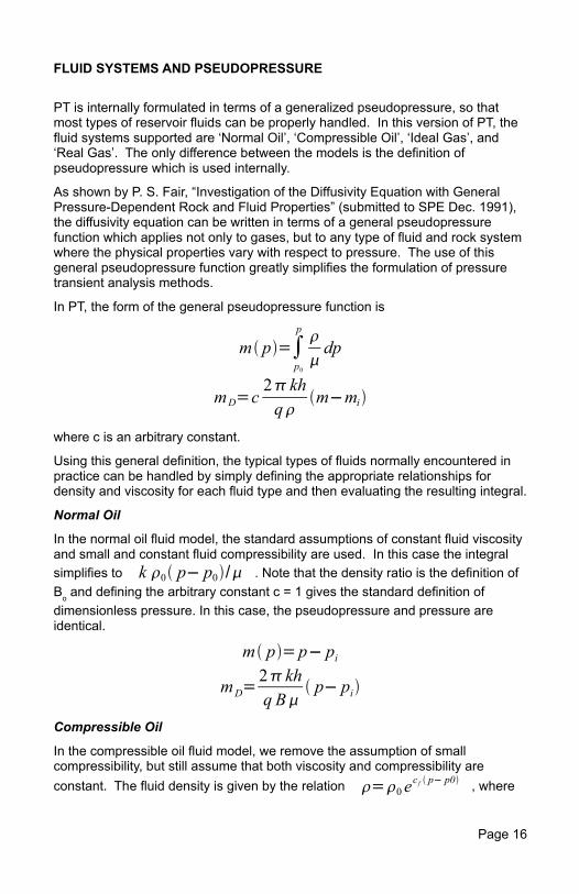
PT is internally formulated in terms of a generalized pseudopressure, so that most types of reservoir fluids can be properly handled. In this version of PT, the fluid systems supported are ‘Normal Oil’, ‘Compressible Oil’, ‘Ideal Gas’, and ‘Real Gas’. The only difference between the models is the definition of pseudopressure which is used internally.

As shown by P. S. Fair, “Investigation of the Diffusivity Equation with General Pressure-Dependent Rock and Fluid Properties” (submitted to SPE Dec. 1991), the diffusivity equation can be written in terms of a general pseudopressure function which applies not only to gases, but to any type of fluid and rock system where the physical properties vary with respect to pressure. The use of this general pseudopressure function greatly simplifies the formulation of pressure transient analysis methods.

In PT, the form of the general pseudopressure function is

m p=∫p0

p dp

mD=c2 khq

m−mi

where c is an arbitrary constant.

Using this general definition, the typical types of fluids normally encountered in practice can be handled by simply defining the appropriate relationships for density and viscosity for each fluid type and then evaluating the resulting integral.

Normal Oil

In the normal oil fluid model, the standard assumptions of constant fluid viscosity and small and constant fluid compressibility are used. In this case the integral simplifies to k 0 p− p0/ . Note that the density ratio is the definition of Bo and defining the arbitrary constant c = 1 gives the standard definition of dimensionless pressure. In this case, the pseudopressure and pressure are identical.

m p=p− pi

mD=2 khq B

p− pi

Compressible Oil

In the compressible oil fluid model, we remove the assumption of small compressibility, but still assume that both viscosity and compressibility are constant. The fluid density is given by the relation =0 e

c f p− p0 , where

Page 16

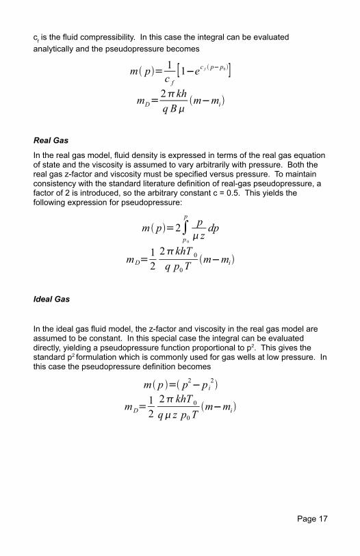
cf is the fluid compressibility. In this case the integral can be evaluated analytically and the pseudopressure becomes

m p= 1c f

[1−ec f p− p0 ]

mD=2khq B

m−mi

Real Gas

In the real gas model, fluid density is expressed in terms of the real gas equation of state and the viscosity is assumed to vary arbitrarily with pressure. Both the real gas z-factor and viscosity must be specified versus pressure. To maintain consistency with the standard literature definition of real-gas pseudopressure, a factor of 2 is introduced, so the arbitrary constant c = 0.5. This yields the following expression for pseudopressure:

m p=2∫p 0

p p zdp

mD=122khT 0q p0T

m−mi

Ideal Gas

In the ideal gas fluid model, the z-factor and viscosity in the real gas model are assumed to be constant. In this special case the integral can be evaluated directly, yielding a pseudopressure function proportional to p2. This gives the standard p2 formulation which is commonly used for gas wells at low pressure. In this case the pseudopressure definition becomes

m p = p2−p i2

mD=122 khT 0q z p0T

m−mi

Page 17

MULTIPLE RATES

Since many tests have varying rates, PT is setup to automatically handle up to 10 rate variations before the start of a well test. This does not mean that data from all of the time periods can be analyzed on one plot. PT allows the analysis of data from only a single constant rate flow period at a time.

However, in order to properly evaluate pressure data it is important that the significant rate history be used in the analysis, since rate variations prior to the start of a test can cause the test data to deviate significantly from the ideal case where the rate is maintained constant.

For type curve analysis, the use of equivalent time is the only choice, since the type curves themselves cannot be easily modified. For classical analysis methods, the method itself defines how the rates are accounted for, for example, the Horner method assumes a constant flow rate prior to a shut-in period, where the rate is known to be zero. In the Adjust and Compare analysis, the rate variations are automatically handled by the use of superposition, so the resulting theoretical curves should be exact.

It should be noted that in PT, all tests are considered to have multiple rates. Drawdown tests are handled internally as multiple rate test with only a single flow period, buildup tests are handled as multiple rate tests with 2 flow periods (the second rate is zero), etc.

In general, the data needed to properly specify the rate variation before the start of the test is a sequence of times and rates entered into the Rate Table on Rate and Pressure Tab in the Test Data window. Note that the time entered here should be the total elapsed time, not the duration of the rate period. Note that the final rate period always has an ending time specified as ‘END’, indicating that the rate lasts until the end of the test.

For example a typical buildup test where the well is produced at a rate of 100 BOPD for 10000 hours prior to shut-in would be entered as 2 rate periods:

10000 100END 0

In general, multiple rate periods would be specified by a sequence of entries as follows:

<ending time of rate1> <rate1><ending time of rate2> <rate2>

...END <rateN>

In this version of PT, a total of 10 rate variations can be represented for any test.

Page 18

USER DEFINED UNITS

In order to accomdate the various measurement units systems in use throughtout the pertroleum industry, PT supports both US and SI standard units systems, as well as user defined units. The default units system is set on the Data window, General Tab by selecting the desired radio button. Note that US standard oilfield units is the default when PT is started.

In the US unit system, volumes are expressed in barrels, pressure in psi, length in feet, viscosity in centipoise, and permeability in millidarcies. In the SI unit system, volume is in cubic meters, pressure in kilopascals, length in meters, viscosity in pascal-seconds, and permeability in square micrometers. In all systems, compressibility is expressed in reciprocal pressure units and time is in hours.

Unfortunately, not all well test data use either unit system in its pure form and units conversion is a chore that is best relegated to computer software. For this reason, PT incorporates a flexible user defined units system which allows the use of any particular units for any test. Internally, PT is written in the so-called ‘Darcy’ units, where volume is in cubic centimeters, pressure is in atmospheres, length in centimeters, viscosity in centipoise, and permeability in Darcies.

To use the user defined units features in PT, the user must enter the appropriate units information on the General Data Tab of the Test Data window. The required input consists of the name of the unit and a conversion factor to be used in the units conversion calculations. The name is used for display purposes only.

The units conversion factor for each unit is the number of units per equivalent Darcy unit. PT will automatically apply these factors in all calculations. The default standard units systems are as folows:

US UnitsPressure psi 14.696 psi/atmLength ft 0.032808 ft/cmVolume bbl 6.28981e-6 bbl/cm3

Permeability md 1000 md/DViscosity cp 1 cp/cp

SI UnitsPressure kPa 1013.25 kPa/atmLength m 0.01 m/cmVolume m3 1.0e-6 m3/cm3

Permeability µm 0.986923 µm/DViscosity Pa.s 1000.0 Pa.s/cp

Page 19

IMPORTING PRESSURE DATA

In order to more directly use data obtained from service companies in computer files, PT 3.0 and later versions implement a reasonably flexible data import mechanism. You can directly import pressure or casing pressure/fluid level data from Echometer® *.exp files, as well as pressure data from text files in a general columnar format. Version 3.1 and higher also support enhanced data editing capabilities which are explained later in this document.

The data import feature of PT is accessed from the Test Data dialog, Rates/Pressures Tab. When the mouse cursor is over the Pressures table, pressing the right mouse button will display a pop-up menu with 3 choices: Import Echometer BHP Data, Import Echometer Data, and Import BHP Data. The first option will allow importing only the calculated BHP data from an Echometer® *.exp file, while the second option will import the surface pressure and fluid level data from an Echometer® *.exp file. The third option allows importing BHP data from a wide range of service companies, as long as the data is in a columnar format.

After selecting the type of data to import, a file directory dialog will be displayed. Select or type the name of the file to import and press the Open button. For the Echometer® data files, the data will be automatically imported and will appear in the Pressure table.

For the Import BHP Data option, an Import BHP Data dialog box will appear showing some information about the file and allowing choices to control the amount and format of the data to be imported. The lower part f the dialog shows a File Preview with line numbers for reference. In the top portion, you can specify how many lines at the top of the file to skip (Skip 1st __ lines), which columns contain the time and pressure data (Time Column and Pressure Column), as well as the Time Format used in the file. If you have a large file, it is also possible to specify Data Thinning parameters to avoid importing enormous amounts of data. The default values of Max DT = 1 hr and Min DP = 1 psi mean that you want to import only pressure points that change by 1 psi or more, but at least 1 point every hour.

When you have set the parameters, press the Import button to import the data. (You can also press Cancel to abort.) If too much data was found in the file, a message will be displayed suggesting that the data thinning parameters be used. Simply select the import option again from the pop-up menu and try again. Each time that you import data, the imported data replaces all of the data currently loaded for the test.

Page 20

ECHOMETER® DATA ANALYSIS

In many beam pumped wells, it is impractical to directly measure bottom hole pressures, since the rod string precludes running a wireline pressure gage. For this reason, bottom hole pressures are often measured indirectly using surface casing pressure and acoustically measured fluid level data. Additional information concerning the acquisition of this data can be obtained from:

The Echometer Co.5001 Ditto Lane

Witchita Falls, Texas 76302USA.

PT 4.0 now supports an analysis method especially formulated for Echometer data. Basically, a new well model has been introduced into the standard well testing equations which allows the casing pressure and fluid level to be predicted directly from the pressure transient equations, so that the raw data can be analyzed directly. This reduces error in the analysis and also leads to a more reliable analysis, since more data is being used. For more technical details of this analysis method, contact The ComPort Computing Co.

To implement the new method, several changes to PT were made for additional data requirements and a new item was added to the Analysis menu. On the test data screen, an Echometer check box has been added, along with a fluid gradient parameter. To specify a Echometer-type well test, simply check the box and enter the estimated fluid gradient in psi/ft.

In addition, for an Echometer well test, the data entry table has been changed to allow the input of both casing pressure and fluid level data versus time as shown below. If a data file is available from Echometer (a file with an extension of *.exp), the data can be automatically imported from the file by positioning the mouse over the Pressure table, pressing the right mouse button and choosing Import Echometer Data from the pop-up menu. Alternatively, choosing Import Echometer BHP Data will import only the estimated bottom hole pressure data from the file.

Once the data has been entered, standard analyses (Classical, Log-log Type Curves, Adjust and Compare) can be performed as detailed in the users manual. For these analyses, the bottom hole pressure is estimated from the fluid gradient, casing pressure and fluid level data in a straight forward manner.

To perform an Echometer analysis, select Echometer from the Analysis menu. An analysis window will be opened as shown below. Note that the upper curve and data points in red represent the fluid level in the well, while the lower data points and curve in blue represent the casing pressure. Two additional parameters are shown on the Well Tab and a weighting factor appears at the bottom right side of the screen.

Just as with the Adjust and Compare method, the analysis consists of adjusting the reservoir and well parameters to obtain the best match to the data. This is done in the same manner as in the Adjust and Compare Analysis. Please refer to

Page 21

that section of the user’s manual for details.

A brief explanation of the additional parameters is also in order. First, in order to compute the fluid level and casing pressure from the well testing equations, some additional parameters on the Well Tab are needed. The first, labeled CD/CLD is the ratio of the wellbore storage to the liquid wellbore storage and is usually about 0.9 to 1.0 if there is gas present in the annulus. A second parameter, labeled Fgi, represents the gas fraction in the initil liquid column in the annulus. Normally this parameter is small, but in wells producing large quantities of annulus gas, may be close to 1.0. Finally there is a parameter labeled DXi that represents the initial fluid column height. In a “pumped off” well, this would correspond to the distance between the pump and the producing interval.

Since this analysis method requires fitting 2 simultaneous data sets, casing pressure in psi and fluid level in feet, a relative weighting factor, labeled Fld Lvl Weight, is also needed. The value of this factor should reflect the relative accuracy of the measurements. Theoretically, the value should be computed by dividing the precision of the casing pressure measurements by the sum of the precisions of the casing pressure and fluid level measurements, converted to psi with the fluid gradient.

In other words, if the fluid level is measured with an accuracy of +/-5 ft and the fluid gradient is 0.35 psi/ft, the fluid level precision is (5 ft)(0.4 psi/ft) = 2.0 psi. If the casing pressure is measured with a precision of +/-0.1 psi, then the weighting factor should be (0.1)/(0.1 + 2.0) = 0.0476. Tests indicate that values in the range of 0.01 to 0.1 are typical and the results are not extremely sensitive to the exact value in most cases.

Page 22

GAGE DATA EDITING

PT 3.1 and later versions contain an improved graphical means of editing raw gage data to delete extraneous pressure measurements. It is now possible to import pressure gage data (as described earlier), view the data on the screen, select any extraneous data points or thin the data, and automatically delete the selected data points. These editing features are available from the Analysis | Classical | Cartesian window by pressing the right mouse button.

When the right mouse button is pressed with the mouse pointer over the plot region of the Cartesian Analysis window, a pop-up menu should appear which has 2 choices: Thin Data and Delete Inactive Data.

Selecting Thin Data presents a dialog on which data thinning parameters can be entered. The Min DP parameter determines the minimum acceptable pressure difference between points. For example, if Min DP = 10 psi, then adjacent data points with a pressure difference less than 10 psi will be purged. The Max DT parameter specifies the maximum time increment between data points. For example, if Max DT = 2 hours, then at least 1 data point every 2 hours will be retained, even if the pressure difference is less than that specified by Min DP. Selecting Ok will mark as inactive the data points to be thinned. Note that Thin Data does not delete the points, but only marks them as inactive.

Delete Inactive Data removes all inactive data points (colored gray on the screen). After deleting the points, it is necessary to go to the Data window and press the Update button for the changes to be registered in memory.

Page 23

PRESSURE TRANSIENT ANALYSIS TUTORIAL

This section of the User’s Guide describes step-by-step how actual pressure transient data can be analyzed using PT 3.0 or later versions. Included on the distribution diskette are several pressure transient data files. These should have been automatically installed along with PT. The test data in these files was extracted from the literature, as referenced in the test title.

Note that to a large extent pressure transient analysis is subjective. Without knowing in advance the exact reservoir model and wellbore effects, it may be possible to obtain several different analyses results for the same data, none of which can be proven to be correct. Therefore, The ComPort Computing Company cannot vouch for the results obtained from the analyses. The analyses shown here are for illustrative purposes only, not to dispute results obtained elsewhere.

In the following sections you will be guided through the evaluation of a published set of pressure transient data. The user is encouraged to perform the steps in these analyses while reading this manual. This will familiarize you with the mechanics of using the PT software and may also provide some valuable insight into a workable approach to the evaluation of actual data.

Selecting and Loading Data

To begin the analysis of a typical data set, start PT by selecting it from the Start Menu (ie. with the mouse, press the Start button, select Programs, select the PT 4.0 group, then select PT40. This should start the program with a blank window, since no data has yet been loaded.

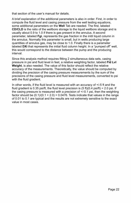
To load the data set that we will use in this example, select File | Open from the menu, then choose TEST1.DAT from the list of files displayed. Either double-click the file name with the mouse, or select the file and then select OK. You should see the Test Data window for this well test as shown on the following page.

On the General Data Tab, note that this is an oil well, the US units system is used, and assorted data has been entered. The units conversion factors should all be set to their default values.

The rest of the test data can also be viewed by clicking on the various tabs for each category. The fluid PVT data is on the tab labeled PVT and the rate and pressure data is found on the tab labeled Rates/Pressures. Note that a Normal Oil fluid system has been selected and the necessary data has been entered for viscosity, total compressibility and formation volume factor. The remaining items are not used for this type of fluid. In addition, you can see that there is one rate defined, since this is a drawdown test. The pressure data consists of 25 points between 0 and 12 hours.

If we needed to make changes to the data, any needed editing could be done on this window. In this case, however, the data should already be correct, so we may proceed with our analysis.

Page 24

Preliminaries - Log-log Analysis

Now that the data for the test has been loaded, let’s take a look at it. While we could jump directly to the Classical or Adjust and Compare analysis techniques, it is often enlightening to view the data to get an idea of the characteristics of the data we are dealing with. For this purpose, a log-log data plot is usually extremely useful.

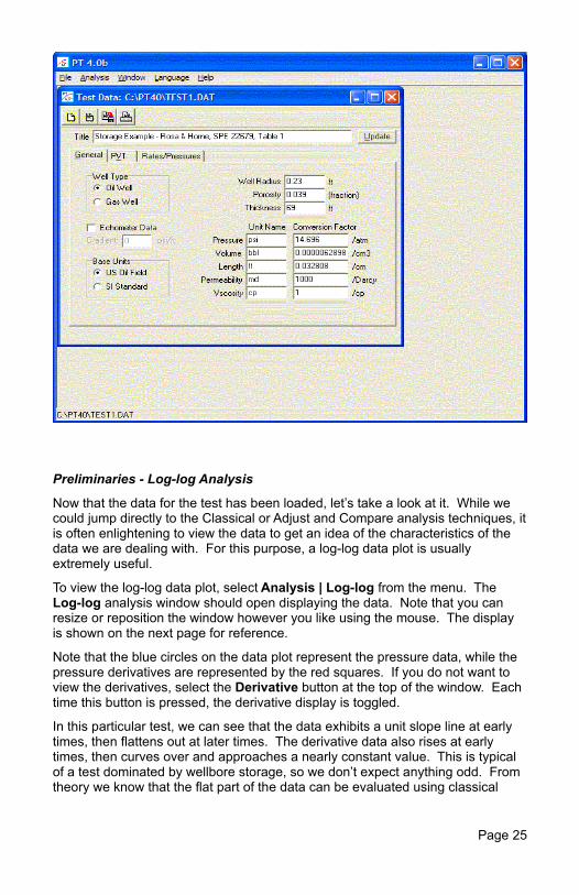
To view the log-log data plot, select Analysis | Log-log from the menu. The Log-log analysis window should open displaying the data. Note that you can resize or reposition the window however you like using the mouse. The display is shown on the next page for reference.

Note that the blue circles on the data plot represent the pressure data, while the pressure derivatives are represented by the red squares. If you do not want to view the derivatives, select the Derivative button at the top of the window. Each time this button is pressed, the derivative display is toggled.

In this particular test, we can see that the data exhibits a unit slope line at early times, then flattens out at later times. The derivative data also rises at early times, then curves over and approaches a nearly constant value. This is typical of a test dominated by wellbore storage, so we don’t expect anything odd. From theory we know that the flat part of the data can be evaluated using classical

Page 25

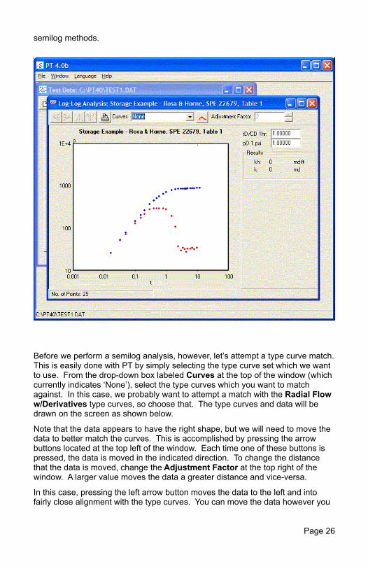
semilog methods.

Before we perform a semilog analysis, however, let’s attempt a type curve match. This is easily done with PT by simply selecting the type curve set which we want to use. From the drop-down box labeled Curves at the top of the window (which currently indicates ‘None’), select the type curves which you want to match against. In this case, we probably want to attempt a match with the Radial Flow w/Derivatives type curves, so choose that. The type curves and data will be drawn on the screen as shown below.

Note that the data appears to have the right shape, but we will need to move the data to better match the curves. This is accomplished by pressing the arrow buttons located at the top left of the window. Each time one of these buttons is pressed, the data is moved in the indicated direction. To change the distance that the data is moved, change the Adjustment Factor at the top right of the window. A larger value moves the data a greater distance and vice-versa.

In this case, pressing the left arrow button moves the data to the left and into fairly close alignment with the type curves. You can move the data however you

Page 26

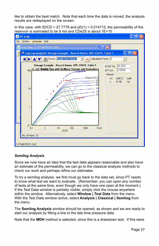
like to obtain the best match. Note that each time the data is moved, the analysis results are redisplayed on the screen.

In this case, with tD/CD = 27.7778 and pD(1) = 0.014715, the permeability of the reservoir is estimated to be 9 md and CDe2S is about 1E+10

Semilog Analysis

Since we now have an idea that the test data appears reasonable and also have an estimate of the permeability, we can go to the classical analysis methods to check our work and perhaps refine our estimates.

To try a semilog analysis, we first must go back to the data set, since PT needs to know what test we want to evaluate. (Remember, you can open any number of tests at the same time, even though we only have one open at the moment.). If the Test Data window is partially visible, simply click the mouse anywhere within the window. Alternatively, select Window | Test Data from the menu. With the Test Data window active, select Analysis | Classical | Semilog from the menu.

The Semilog Analysis window should be opened, as shown and we are ready to start our analysis by fitting a line to the late time pressure data.

Note that the MDH method is selected, since this is a drawdown test. If this were

Page 27

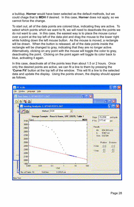
a buildup, Horner would have been selected as the default methods, but we could chage that to MDH if desired. In this case, Horner does not apply, so we cannot force the change.

To start out, all of the data points are colored blue, indicating they are active. To select which points which we want to fit, we will need to deactivate the points we do not want to use. In this case, the easiest way is to place the mouse cursur over a point at the top left of the data plot and drag the mouse to the lower right while holding down the left mouse button. As the mouse is moved, a rectangle will be drawn. When the button is released, all of the data points inside the rectangle will be changed to gray, indicating that they are no longer active. Alternatively, clicking on any point with the mouse will toggle the color to gray, deactivating the point. Clicking on the point again will toggle its color back to blue, activating it again.

In this case, deactivate all of the points less than about 1.5 or 2 hours. Once only the desired points are active, we can fit a line to them by pressing the ‘Curve Fit’ button at the top left of the window. This will fit a line to the selected data and update the display. Using the points shown, the display should appear as follows.

Page 28

Note that the slope of the line and the value of pressure at 1 hour are shown and the permeability and skin have also been automatically calculated based on the position of the line. If you want to manually adjust the line, the slope and intercept can be entered. You can also change which points are active and fit another line to the data.

In this case, however, it appears that the line is pretty reasonable, since the standard deviation (at the bottom of the window) is less than 0.4 psi using 10 data points, so we will leave it alone.

Note that the permeability is estimated to be 9.05 md and the skin is estimated to be about 5.7. This is encouraging, since the permeability agrees fairly well with the estimate from the log-log analysis earlier.

Note also the buttons that appear on the bottom part of the right panel in the window. These can be used to change the scale and display to view the data. Pressing the Position buttons slides the scale right and left or up and down, while pressing the Divisions buttons increases or decreases the number of divisions shown. By using these, the graph can be adjusted to suit your tastes, zooming in or out on parts of the data as desired. The position of the plot on the display has no effect on the analysis results.

Wellbore Storage - Cartesian Analysis

In this well test, we noted from the log-log plot that the early time was dominated by wellbore storage and that the early time data appears to form a unit slope line. This means that a cartesian graph of the early time data should be linear and that we can use Cartesian Analysis to determine the wellbore storage constant.

To perform a Cartesian Analysis, activate the Test Data window and select Analysis | Classical | Cartesian from the menu. The Cartesian Analysis window will be displayed.

Note that the Method selected at the top of the window is Wellbore Storage. If we were looking at late time data, the Reservoir Limit method could be selected instead. In most cases, however, we will want wellbore storage, as in this case.

Since we want to look at the early time data, it is necessary to zoom the plot to show all of the early points. First, we will deactivate the late time points (greater than about 1 hour) by dragging the mouse across them. Then select the appropriate buttons to decrease the number of X-Axis Divisions to expand the graph horizontally. As the graph expands, it appears that more of the points are not linear, so we deselect those, also, until the only remaining points are at times less than about 0.1 hours. Pressing the ‘Curve Fit’ button at the upper left fits a line to the remaining points as shown.

Note that the standard deviation is about 0.64 psi, which appears acceptable. The wellbore storage is also estimated as 0.00887 bbl/psi (which could be checked against well tubular data, if we had any) and the dimensionless storage is estimated to be about 8306.

Since we estimated the skin to be about 5.8 from the semilog analysis, we can also check the CDe2S parameter with our match on the log-log plot. Using 8306

Page 29

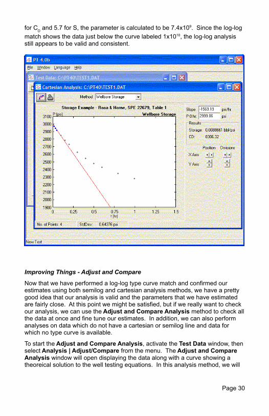
for CD and 5.7 for S, the parameter is calculated to be 7.4x109. Since the log-log match shows the data just below the curve labeled 1x1010, the log-log analysis still appears to be valid and consistent.

Improving Things - Adjust and Compare

Now that we have performed a log-log type curve match and confirmed our estimates using both semilog and cartesian analysis methods, we have a pretty good idea that our analysis is valid and the parameters that we have estimated are fairly close. At this point we might be satisfied, but if we really want to check our analysis, we can use the Adjust and Compare Analysis method to check all the data at once and fine tune our estimates. In addition, we can also perform analyses on data which do not have a cartesian or semilog line and data for which no type curve is available.

To start the Adjust and Compare Analysis, activate the Test Data window, then select Analysis | Adjust/Compare from the menu. The Adjust and Compare Analysis window will open displaying the data along with a curve showing a theoreical solution to the well testing equations. In this analysis method, we will

Page 30

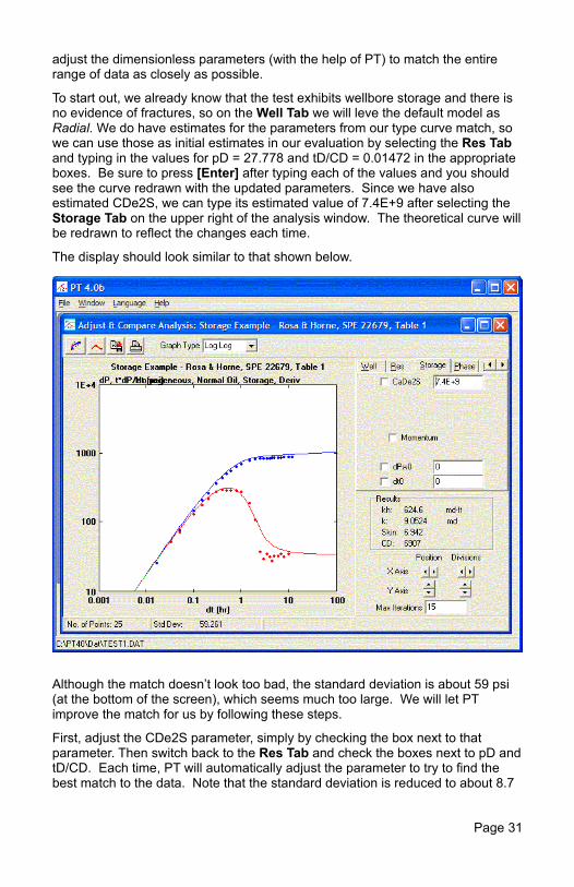
adjust the dimensionless parameters (with the help of PT) to match the entire range of data as closely as possible.

To start out, we already know that the test exhibits wellbore storage and there is no evidence of fractures, so on the Well Tab we will leve the default model as Radial. We do have estimates for the parameters from our type curve match, so we can use those as initial estimates in our evaluation by selecting the Res Tab and typing in the values for pD = 27.778 and tD/CD = 0.01472 in the appropriate boxes. Be sure to press [Enter] after typing each of the values and you should see the curve redrawn with the updated parameters. Since we have also estimated CDe2S, we can type its estimated value of 7.4E+9 after selecting the Storage Tab on the upper right of the analysis window. The theoretical curve will be redrawn to reflect the changes each time.

The display should look similar to that shown below.

Although the match doesn’t look too bad, the standard deviation is about 59 psi (at the bottom of the screen), which seems much too large. We will let PT improve the match for us by following these steps.

First, adjust the CDe2S parameter, simply by checking the box next to that parameter. Then switch back to the Res Tab and check the boxes next to pD and tD/CD. Each time, PT will automatically adjust the parameter to try to find the best match to the data. Note that the standard deviation is reduced to about 8.7

Page 31

psi, which is much better. In addition, the permeability is estimated at about 9 md and skin at 5.7, which is pretty close to our previous estimates.

But we can do even better. So far we have adjusted the parameters independently. By letting PT perform a nonlinear search, all of the parameters can be adjusted simultaneously, which is a much better numerical technique. Unfortunately, the nature of the data and equations requires that we have a pretty good estimate of the parameters before we turn PT loose. By adjusting the parameters independently, we’ve come pretty close to a match, so PT should be able to do its work from here.

To let PT find a better solution, simply press the ‘Curve Fit’ button at the upper left of the window. PT will search through about 15 iterations of a nonlinear search, updating the curve as it proceeds. When it’s finished, an improved match is obtained, with a standard deviation of about 7.5 psi. Note that the estimates of permeability and skin have changed to about 9.2 md and 6.1 respectively. We can ask PT to continue searching for an improved match by pressing the 'Curve Fit' button repeatedly, or by allowing more iterations by setting Max Iterations to a larger number, like 100. Go ahead and try it.

But, since PT handles much more complex analysis models, we can do even better than this. Note that the derivative data appears to drop too rapidly and flatten out too soon in comparison to the theoretical curve. This might be due to wellbore effects, which we can model.

To model the effect noticed here, we will use a small amount of phase redistribution. Note that since this is a drawdown test, we don’t expect phase redistribution in its normal sense, but instead the efffect is probably due to temperature changes in the wellbore. Discussion of this is beyond the scope of this manual, but the interested reader is referred to the paper referenced in the Appendix. (We could also add momentum effects, but that isn’t needed here.)

To include phase redistribution effects in the theoretical curve, simply go to the Phase Tab and change the Model to Fair. Note that some additional parameters appear to describe the phase redistribution effect and that the curve is redrawn to effect the changes.

Since the amount of phase redistribution is small in this case, first lower the value of CD/CaD from 10 to 1.2, then change the value of CpD from 10 to about 4. Note that the curve shape adjusts each time and now has a much better shape. However adjusting these parameters changed the match, so we go back to the Reservoir Tab and readjust the tD/CD value by unchecking and rechecking the box next to it. At this point the standard deviation has been reduced to about 4.0 psi, which is significant, and the curve has the right overall shape to match the data.

To complete our analysis, we can let PT find a better match for us. First activate the new parameters by going to the Phase Tab and checking the boxes next to CD/CaD and CpD. Then press the ‘Curve Fit’ button again. PT will again adjust all of the parameters for the best match it can find.

Note that the standard deviation has been reduced to about 2.6 psi and that the

Page 32

estimated permeability and skin are now 9.87 md and 6.89 respectively. These estimates are fairly close to our prior estimates, so we can be pretty sure that our analysis is valid. In addition, we have explained the slight deviation in the data by introducing some wellbore effects and also shown that these effects do not substantially change the evaluation results.

As stated before, the purpose of this analysis has been to illustrate the use of PT for evaluating well test data. You can further adjust the parameters or try changing the reservoir model and let PT continue improving the match until you are satisfied that the best match has been obtained.

With about 1000 iterations, you should be able to attain a standard deviatin of about 2.57 psi for this test and the permeability and skin would be around 9.45 md and 6.29 respectively.

Page 33

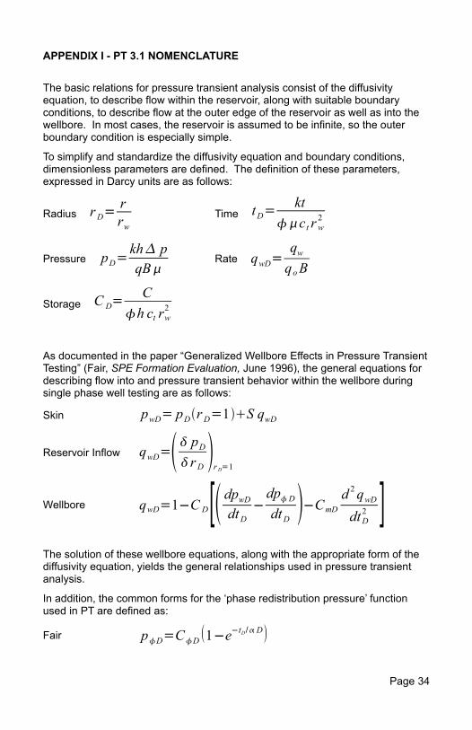
APPENDIX I - PT 3.1 NOMENCLATURE

The basic relations for pressure transient analysis consist of the diffusivity equation, to describe flow within the reservoir, along with suitable boundary conditions, to describe flow at the outer edge of the reservoir as well as into the wellbore. In most cases, the reservoir is assumed to be infinite, so the outer boundary condition is especially simple.

To simplify and standardize the diffusivity equation and boundary conditions, dimensionless parameters are defined. The definition of these parameters, expressed in Darcy units are as follows:

Radius rD=rrw

Time tD=kt

c t rw2

Pressure pD=kh pqB

Rate qwD=qwqoB

Storage C D=C

h ct rw2

As documented in the paper “Generalized Wellbore Effects in Pressure Transient Testing” (Fair, SPE Formation Evaluation, June 1996), the general equations for describing flow into and pressure transient behavior within the wellbore during single phase well testing are as follows:

Skin pwD= pDrD=1S qwD

Reservoir Inflow qwD= pD rD r D=1Wellbore qwD=1−C D[ dpwDdtD

−dpDdtD −CmD d

2qwDdtD2 ]

The solution of these wellbore equations, along with the appropriate form of the diffusivity equation, yields the general relationships used in pressure transient analysis.

In addition, the common forms for the ‘phase redistribution pressure’ function used in PT are defined as:

Fair pD=CD 1−e−tD / D

Page 34

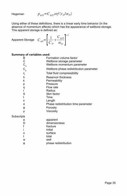
Hegeman pD=CD erf t D/D

Using either of these definitions, there is a linear early time behavior (in the absence of momentum effects) which has the appearance of wellbore storage. This apparent storage is defined as:

Apparent Storage CaD=[ 1C DCD

D ]−1

Summary of variables used:B Formation volume factor C Wellbore storage parameterCm Wellbore momentum parameterC

φWellbore phase redistribution parameter

ct Total fluid compressibilityh Reservoir thicknessk Permeabilityp Pressureq Flow rater RadiusS Skin factort Timex Lengthα Phase redistribution time parameterφ Porosityµ Viscosity

Subscriptsa apparentD dimensionlessf fracturei initialo surfacet totalw wellφ phase redistribution

Page 35

APPENDIX II - AN OVERVIEW OF PRESSURE TRANSIENT METHODS

The mathematical basis of pressure transient analysis lies in the partial differential equations of single phase fluid flow. Since we are concerned mainly with the pressure response at a producing well during time periods when wellbore effects may be important, the radial form of the diffusivity equation is usually used to model the reservoir flow behavior. Since wellbore effects are important, mass and momentum balance relations for fluids in the wellbore describe the wellbore boundary conditions. Since the reservoir is normally extremely large in comparison with the size of the wellbore, an infinite reservoir is often assumed.

In order to keep from solving the equations for every combination of parameters that might be encountered, the equations are generally expressed in terms of dimensionless quantities. Except for a few unusual circumstances, the same set of dimensionless parameters are used throughout well test analysis and are described in Appendix I.

Once the diffusivity equation and the associated boundary conditions are specified in terms of dimensionless variables and a solution is obtained, the process of pressure transient analysis becomes one of determining what values of the dimensionless variables and parameters are needed to achieve a match between the theoretical solutions and the measured data. This can be done in several ways, leading to the three major methods used in pressure transient analysis and implemented in the PT software.

Classical analysis methods rely on the observation that portions of the theoretical pressure solutions form straight lines when plotted versus some type of time related variable. The Cartesian plot is useful at early times, when wellbore storage dominates and inflow from the reservoir is essentially filling the wellbore. It is also useful at very late times, when production is draining the reservoir and the average reservoir pressure is dropping with time. The square root of time plot is useful when transient linear flow dominates, usually due to flow into a vertical fracture intersecting the wellbore. The semilog methods are useful during transient radial flow after wellbore effects have died out. In any of the methods, fitting a straight line to the data is one way to determine the parameters required to make the solution match the data. The slope and intercept of the fitted line are used to compute the physical parameters.

Type curve analysis relies on the observation that the dimensionless time and pressure parameters consist of a constant term multiplied by real time or pressure and the fact that multiplying numbers is equivalent to adding logarithms. When both the theoretical solutions and data are plotted on a log-log graph, sliding the data vertically and horizontally is equivalent to adding or subtracting logarithms and thereby adjusting the constant term of the dimensionless parameters. When a suitable match is obtained visually, the parameters can be determined from the ratio of the real and theoretical parameters at any point on the graph. This is equivalent to fitting a line, except that curves are used and no assumption of linearity in the solution is required.

The adjust and compare method, as implemented in PT, is more direct in

Page 36

determining the parameters of the solution. Instead of changing the problem into one of finding a straight line or matching some set of theoretical curves, the data and theoretical solutions are plotted on the same graph and the parameters of the theoretical solution are adjusted until the best match is obtained. Using this method, we are able to analyze data which exhibit no straight line by any method, as well as in situations where no set of type curves has been prepared. The values of the parameters of the theoretical solution directly determine the desired analysis results.

Page 37

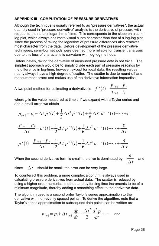
APPENDIX III - COMPUTATION OF PRESSURE DERIVATIVES

Although the technique is usually referred to as "pressure derivatives", the actual quantity used in "pressure derivative" analysis is the derivative of pressure with respect to the natural logarithm of time. This corresponds to the slope on a semi-log plot, which always has more visual curve character than that of a log-log plot, since the process of taking the logarithm of pressure differences also removes most character from the data. Before development of the pressure derivative techniques, semi-log methods were deemed more reliable for transient analyses due to this loss of characteristic curvature with log-log methods.

Unfortunately, taking the derivative of measured pressure data is not trivial. The simplest approach would be to simply divide each pair of pressure readings by the difference in log-time, however, except for ideal data, the resulting values nearly always have a high degree of scatter. The scatter is due to round-off and measurement errors and makes use of the derivative information impractical.

A two point method for estimating a derivative is f ' t =p i1−p it i1−t i

where p is the value measured at time t. If we expand with a Taylor series and add a small error, we obtain

p i1= pit p ' t 12 t 2 p ' ' t 1

6 t3 p ' ' ' t ⋯

pi1−p i t

=p ' t 12 t p ' ' t 1

6 t 2 p ' ' ' t ⋯

t

p ' t =p i1−p i t

−12 t p ' ' t −1

6 t 2 p ' ' ' t ⋯

x

When the second derivative term is small, the error is dominated by t

and

since t should be small, the error can be very large.

To counteract this problem, a more complex algorithm is always used in calculating pressure derivatives from actual data. The scatter is reduced by using a higher order numerical method and by forcing time increments to be of a minimum magnitude, thereby adding a smoothing effect to the derivative data.

The algorithm used is a second order Taylor's series approximation to the derivative with non-evenly spaced points. To derive the algorithm, note that a Taylor's series approximation to subsequent data points can be written as:

p i1= pit i1dpdt

t 2

2d 2 pdt 2

⋯ and

Page 38

p i−1= pi− t i1dpdt

t2

2d 2 pdt 2

−⋯

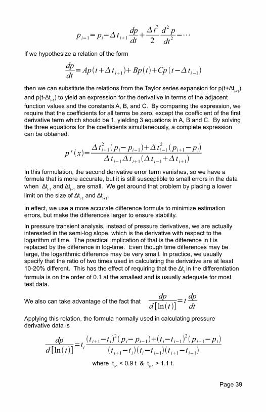
If we hypothesize a relation of the form

dpdt

=Apt t i1Bpt Cp t− ti−1

then we can substitute the relations from the Taylor series expansion for p(t+∆ti+1) and p(t-∆ti-1) to yield an expression for the derivative in terms of the adjacent function values and the constants A, B, and C. By comparing the expression, we require that the coefficients for all terms be zero, except the coefficient of the first derivative term which should be 1, yielding 3 equations in A, B and C. By solving the three equations for the coefficients simultaneously, a complete expression can be obtained.

p ' x= t i1

2 p i− pi−1 ti−12 pi1−p i

t i−1 t i1 t i−1 t i1In this formulation, the second derivative error term vanishes, so we have a formula that is more accurate, but it is still susceptible to small errors in the data when ∆ti-1 and ∆ti+1 are small. We get around that problem by placing a lower limit on the size of ∆ti-1 and ∆ti+1.

In effect, we use a more accurate difference formula to minimize estimation errors, but make the differences larger to ensure stability.

In pressure transient analysis, instead of pressure derivatives, we are actually interested in the semi-log slope, which is the derivative with respect to the logarithm of time. The practical implication of that is the difference in t is replaced by the difference in log-time. Even though time differences may be large, the logarithmic difference may be very small. In practice, we usually specify that the ratio of two times used in calculating the derivative are at least 10-20% different. This has the effect of requiring that the ∆ti in the differentiation formula is on the order of 0.1 at the smallest and is usually adequate for most test data.

We also can take advantage of the fact that dp

d [ lnt ]= t dpdt

Applying this relation, the formula normally used in calculating pressure derivative data is

dpd [ ln t ]

=tit i1−t i

2 p i− pi−1t i−t i−12 p i1−p i

t i1−t iti−t i−1t i1−t i−1where ti-1 < 0.9 t & ti+1 > 1.1 t.

Page 39