Embed Size (px)
DESCRIPTION
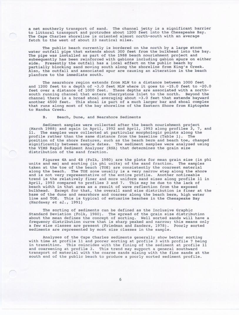
Assessment of Cape Charles Beach in Cape Charles, VA
Citation preview
CAPE'~R:L.§§ .
PUBLIC BEACH ASSESf,tU1J:Nl.REPORT-._!-~ . ;~.f ;.- .
by
C. Scott .lfarda)f/ty Jr.Doniia.A~Mi1tigan.George R. !t'Thomas'.'p
; ....
Virginia Institq,te{~Ofi;Marine S~i~nce'College of Wi[fia.1ft,'ant!:M{l.~. .
..;-., ~.\.~,.- ~ '~" .-.iJ.;IJ:Jf".=,~ -! ..~., - ,..
Gloucester Poznt,,':'¥zrgu'na 23062.. ,.. . .~. ': '
June;:~9.93' .
- - --
1.
A.B.C.
II.
CONTENTS
Page
INTRODUCTION . .1
133
3
. . . .
Background and PurposeLimits of Study Area .
Approach and Methodology
COASTAL SETTING
A.B.C.
Shore Morphology and Sediment TransportBeach, Dune, and Nearshore SedimentsWave Climate . . . . . . . .
368
III. BEACH CHARACTERISTICS AND BEHAVIOR 10
IV.
A.B.
Beach and Nearshore Profiles and Their VariabilityVariability in Shoreline position and Sand Volume
1011
1-2.
Shoreline Position Variability . . . . . .
Beach, Dune, and Nearshore Volume Changes
1121
C. Anthropogenic Impacts to Shoreline Processes 25
WAVE MODELLING AT CAPE CHARLES 25
A.B.C.
RCPWAVE Setup . . . . .
Wave Height Distribution and Wave RefractionLittoral Transport Patterns
252936
39V. CONCLUSIONS
39VI. RECOMMENDATIONS
41VII. REFERENCES.
APPENDIX I. Additional References about LittoralProcesses and Hydrodynamic Modeling
i
FIGURES
Page
Figure 1. site location, Cape Charles, Virginia, Virginia Powerstation at Yorktown, Nandua Creek and Kiptopeke 2
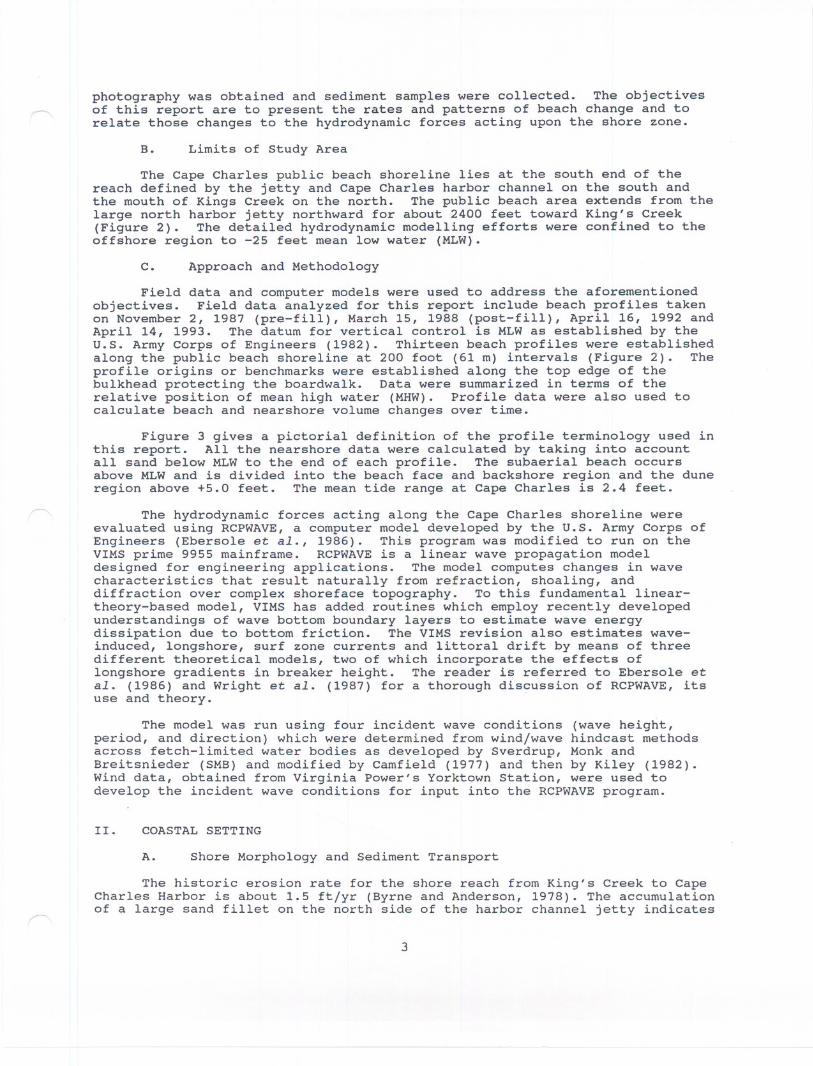
Figure 2. Base map of Cape Charles Beach with profileand cell locations . . . . . . . . . . . . ...... 4
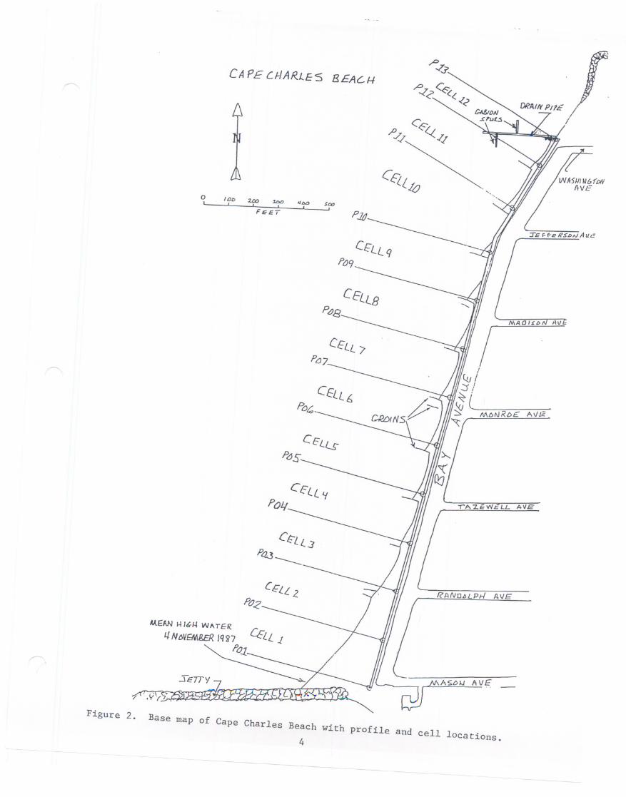
Figure 3. Typical beach profile demonstrating terminologyused in report . . . . . . . . . . . . . . . . 5
Figure 4A. Results of sediment sample analysis for mean size (phi)
Figure 4B. Results of sedimentsample analysisfor sorting (phi) .
7
7
Figure 5. Profile 1 plot depicting changes at Cape Charles Beach .. 12
Figure 6. Profile 2 plot depicting changes at Cape Charles Beach .. 12
Figure 7. Profile 3 plot depicting changes at Cape Charles Beach .. 13
Figure 8. Profile 4 plot depicting changes at Cape Charles Beach .. 13
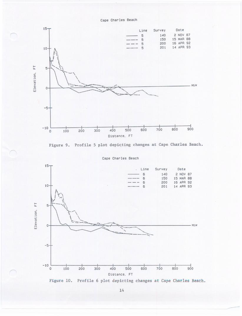
Figure 9. Profile 5 plot depicting changes at Cape Charles Beach .. 14
Figure 10. Profile 6 plot depictingchangesat Cape Charles Beach . . 14
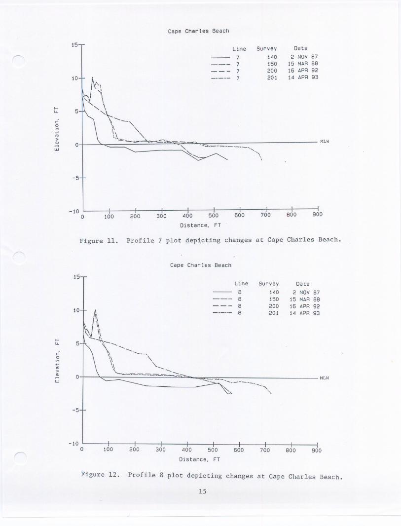
Figure 11. Profile7 plot depictingchangesat Cape CharlesBeach . . 15
Figure 12. Profile 8 plot depicting changes at Cape Charles Beach .. 15
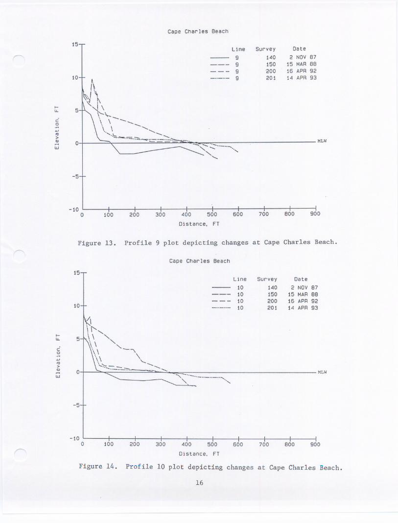
Figure 13. Profile 9 plot depicting changes at Cape Charles Beach .. 16
Figure 14. Profile 10 plot depicting changes at Cape Charles Beach .. 16
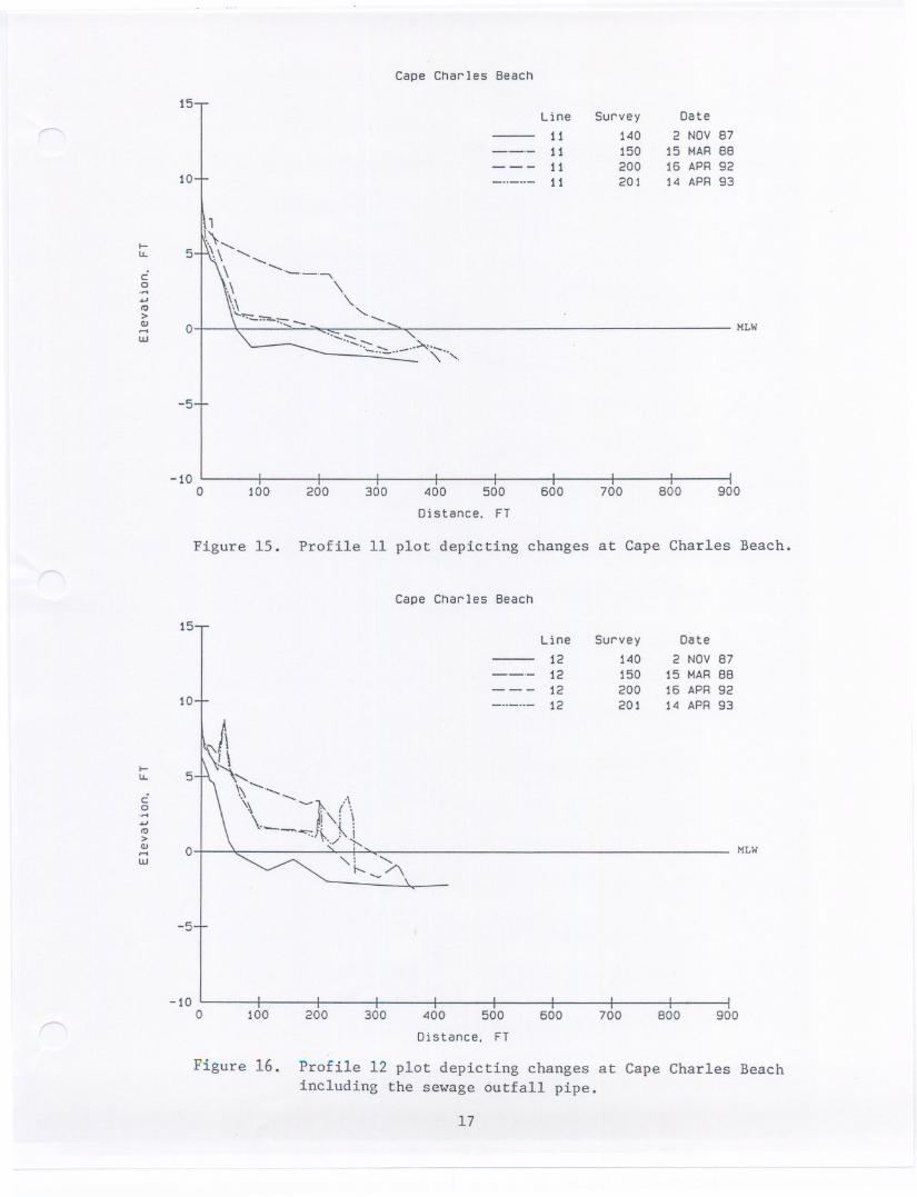
Figure 15. Profile 11 plot depicting changes at Cape Charles Beach.. 17
Figure 16. Profile 12 plot depicting changes at Cape Charles Beachincluding the sewage outfall pipe . . . . . . . . . . . .. 17
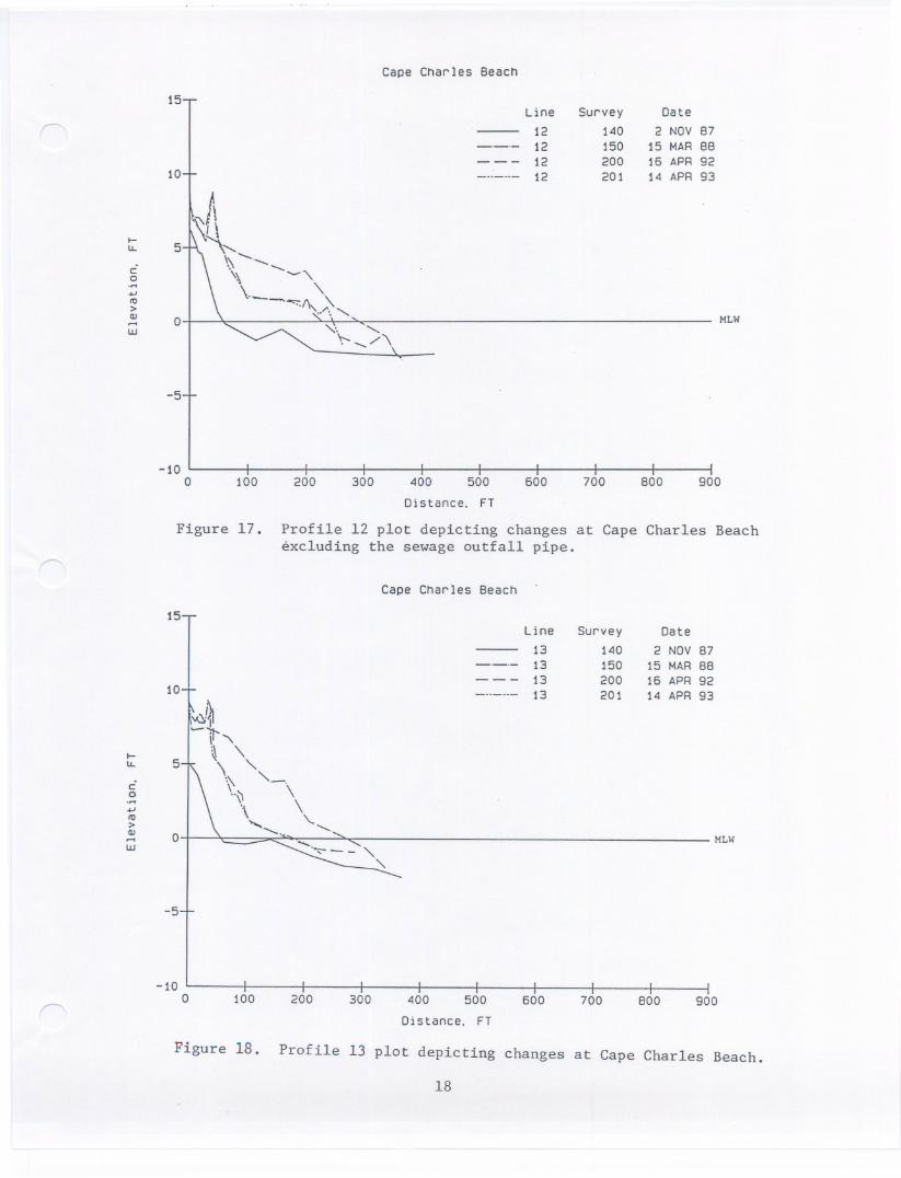
Figure 17. Profile 12 plot depicting changes at Cape Charles Beachexcludingthe sewageoutfallpipe . . . . . . . . . . . .. 18
Figure 18. Profile 13 plot depicting changes at Cape Charles Beach .. 18
Figure 19. Distance of MHW from the baseline . . . . . . . . . . . .. 19
Figure 20. Elevationabove MLW of the base of dune . . . . . . . . . . 20
Figure 21. Distanceto the base of dune from the baseline . . . . . . 20
Figure 22. Subaerial beach volume calculations by cells . . . . . . . 22
Figure 23. Subaerialbeach rate of change . . . . . . . . . . . . . . 22
Figure 24. Volume of sand in dune area relative to the 1987nourishment project . . . . . . . . . . . . . . . . . . . . 23
Figure 25. Volume rate of change in the dune area . . . . . . . . . . 23
ii
Figure 26. Nearshore volume change relative to the 1987nourishment project . . . . . . . .
Figure 27. Volume rate of change in the nearshore region
Figure 28. Summary of volume changes .......
24
24
26
Figure 29. Base map depicting distance to MHW from the baseline . .. 27
Figure 30. Shoreline and offshore bathymetry grid at Cape CharlesBeachusedin the RCPWAVEevaluation. . . . . . . . . .. 28
Figure 31A. Breaking wave height (Hb) (feet) distributionfor the southwest annual modal wave condition ....... 30
Figure 31B. Breaking wave height (Hb) (feet) distributionfor the west annual modal wave condition ....... 30
Figure 32A. Breaking wave height (Hb) (feet) distributionfor the northwest annual modal wave condition ....... 31
Figure 32B. Breaking wave height (Hb) (feet) distributionfor the northwest storm wave condition ..... 31
Figure 33A. Regional wave vector plot for the west modal condition .. 32
Figure 33B. Local wave vector plot for the west modal condition . . .. 32
Figure 34A. Regional wave vector plot for the southwest modal condition 33
Figure 34B. Local wave vector plot for the southwest modal condition . 33
Figure 35A. Regional wave vector plot for the northwest modal condition 34
Figure 35B. Local wave vector plot for the northwestmodal condition . 34
Figure 36A. Regional wave vector plot for the northwest storm condition 35
Figure 36B. Local wave vector plot for the northwest storm condition . 35
Figure 37A. Gradient of alongshore energy flux (dQ/dy)(cy/hr)for the west modal condition . . . . . . . . . . ..... 37
Figure 37B. Gradient of alongshore energy flux (dQ/dy)(cy/hr)for the southwestmodal condition. . . . . . . . ..... 37
Figure 38A. Gradient of alongshore energy flux (dQ/dy)(cy/hr)forthe northwestmodalcondition. . . . . . . . ..... 38
Figure 38B. Gradient of alongshore energy flux (dQ/dy)(cy/hr)for the northwest storm condition . . . . . . . . ..... 38
iii
Table 1.
Table 2.
Table 3.
Table 4.
TABLES
Morphologic features at which sediment samplesare located . . . . . . . . . . . . . . . ~ . .....
Cape Charles hindcasted wave data by year and direction
RCPWAVE input wave conditions ..........
Page
8
10
10
Cape Charles volume changes relative to the1987 beach nourishment project . . . . . . . . . . . . . . . 25
iv
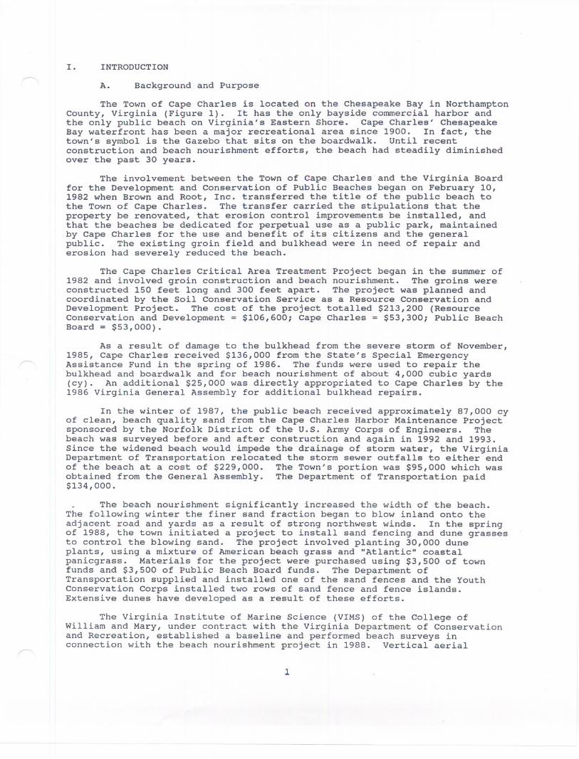
I. INTRODUCTION
A. Background and Purpose
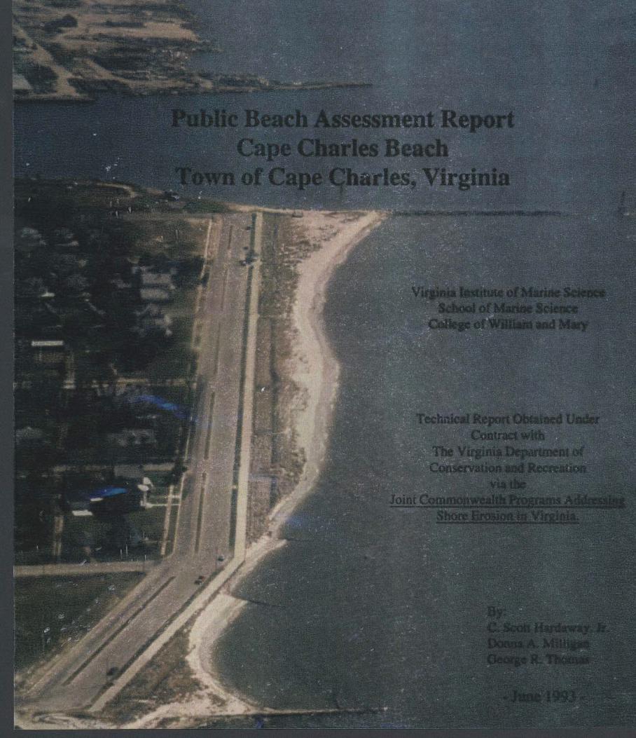
The Town of Cape Charles is located on the Chesapeake Bay in NorthamptonCounty, Virginia (Figure 1). It has the only bays ide commercial harbor andthe only public beach on Virginia's Eastern Shore. Cape Charles' ChesapeakeBay waterfront has been a major recreational area since 1900. In fact, thetown's sYmbol is the Gazebo that sits on the boardwalk. Until recentconstruction and beach nourishment efforts, the beach had steadily diminishedover the past 30 years.
The involvement between the Town of Cape Charles and the Virginia Boardfor the Development and Conservation of Public Beaches began on February 10,1982 when Brown and Root, Inc. transferred the title of the public beach tothe Town of Cape Charles. The transfer carried the stipulations that theproperty be renovated, that erosion control improvements be installed, andthat the beaches be dedicated for perpetual use as a public park, maintainedby Cape Charles for the use and benefit of its citizens and the generalpublic. The existing groin field and bulkhead were in need of repair anderosion had severely reduced the beach.
The Cape Charles Critical Area Treatment Project began in the summer of1982 and involved groin construction and beach nourishment. The groins wereconstructed 150 feet long and 300 feet apart. The project was planned andcoordinated by the Soil Conservation Service as a Resource Conservation andDevelopment Project. The cost of the project totalled $213,200 (ResourceConservation and Development = $106,600; Cape Charles = $53,300; Public BeachBoard = $53,000).
As a result of damage to the bulkhead from the severe storm of November,1985, Cape Charles received $136,000 from the State's Special EmergencyAssistance Fund in the spring of 1986. The funds were used to repair thebulkhead and boardwalk and for beach nourishment of about 4,000 cubic yards(cy). An additional $25,000 was directly appropriated to Cape Charles by the1986 Virginia General Assembly for additional bulkhead repairs.
In the winter of 1987, the public beach received approximately 87,000 cyof clean, beach quality sand from the Cape Charles Harbor Maintenance Projectsponsored by the Norfolk District of the U.S. Army Corps of Engineers. Thebeach was surveyed before and after construction and again in 1992 and 1993.Since the widened beach would impede the drainage of storm water, the VirginiaDepartment of Transportation relocated the storm sewer outfalls to either endof the beach at a cost of $229,000. The Town's portion was $95,000 which wasobtained from the General Assembly. The Department of Transportation paid$134,000.
The beach nourishment significantly increased the width of the beach.The following winter the finer sand fraction began to blow inland onto theadjacent road and yards as a result of strong northwest winds. In the springof 1988, the town initiated a project to install sand fencing and dune grassesto control the blowing sand. The project involved planting 30,000 duneplants, using a mixture of American beach grass and "Atlantic" coastalpanicgrass. Materials for the project were purchased using $3,500 of townfunds and $3,500 of Public Beach Board funds. The Department ofTransportation supplied and installed one of the sand fences and the YouthConservation Corps installed two rows of sand fence and fence islands.Extensive dunes have developed as a result of these efforts.
The Virginia Institute of Marine Science (VIMS) of the College ofWilliam and Mary, under contract with the Virginia Department of Conservationand Recreation, established a baseline and performed beach surveys inconnection with the beach nourishment project in 1988. Vertical aerial
1
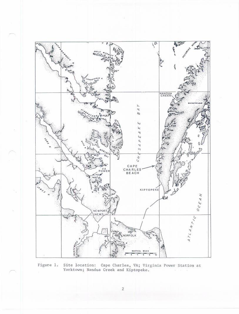
Figure 1. Site location: Cape Charles, VA; Virginia Power Station atYorktown; Nandua Creek and Kiptopeke.
2
photography was obtained and sediment samples were collected. The objectivesof this report are to present the rates and patterns of beach change and torelate those changes to the hydrodynamic forces acting upon the shore zone.
B. Limits of study Area
The Cape Charles public beach shoreline lies at the south end of thereach defined by the jetty and Cape Charles harbor channel on the south andthe mouth of Kings Creek on the north. The public beach area extends from thelarge north harbor jetty northward for about 2400 feet toward King's Creek(Figure 2). The detailed hydrodynamic modelling efforts were confined to theoffshore region to -25 feet mean low water (MLW).
C. Approach and Methodology
Field data and computer models were used to address the aforementionedobjectives. Field data analyzed for this report include beach profiles takenon November 2, 1987 (pre-fill), March 15, 1988 (post-fill), April 16, 1992 andApril 14, 1993. The datum for vertical control is MLW as established by theu.s. Army Corps of Engineers (1982). Thirteen beach profiles were establishedalong the public beach shoreline at 200 foot (61 m) intervals (Figure 2). Theprofile origins or benchmarks were established along the top edge of thebulkhead protecting the boardwalk. Data were summarized in terms of therelative position of mean high water (MHW). Profile data were also used tocalculate beach and nearshore volume changes over time.
Figure 3 gives a pictorial definition of the profile terminology used inthis report. All the nearshore data were calculated by taking into accountall sand below MLW to the end of each profile. The subaerial beach occursabove MLW and is divided into the beach face and backshore region and the duneregion above +5.0 feet. The mean tide range at Cape Charles is 2.4 feet.
The hydrodynamic forces acting along the Cape Charles shoreline wereevaluated using RCPWAVE, a computer model developed by the u.s. Army Corps ofEngineers (Ebersole et al., 1986). This program was modified to run on theVIMS prime 9955 mainframe. RCPWAVE is a linear wave propagation modeldesigned for engineering applications. The model computes changes in wavecharacteristics that result naturally from refraction, shoaling, anddiffraction over complex shoreface topography. To this fundamental linear-theory-based model, VIMS has added routines which employ recently developedunderstandings of wave bottom boundary layers to estimate wave energydissipation due to bottom friction. The VIMS revision also estimates wave-induced, longshore, surf zone currents and littoral drift by means of threedifferent theoretical models, two of which incorporate the effects oflongshore gradients in breaker height. The reader is referred to Ebersole etal. (1986) and Wright et al. (1987) for a thorough discussion of RCPWAVE, itsuse and theory. .
The model was run using four incident wave conditions (wave height,period, and direction) which were determined from wind/wave hindcast methodsacross fetch-limited water bodies as developed by Sverdrup, Monk andBreitsnieder (SMB) and modified by Camfield (1977) and then by Kiley (1982).Wind data, obtained from Virginia Power's Yorktown station, were used todevelop the incident wave conditions for input into the RCPWAVE program.
II. COASTAL SETTING
A. Shore Morphology and Sediment Transport
The historic erosion rate for the shore reach from King's Creek to CapeCharles Harbor is about 1.5 ft/yr (Byrne and Anderson, 1978). The accumulationof a large sand fillet on the north side of the harbor channel jetty indicates
3
~/N P/1£ f/
Figure 2. Base map of Cape Charles Beach with profile and cell locations.4
CA PE CHARLES BEAC-I-I
ol I {)b zoo k>D IICD SDtJ
J I ~~IFEEl
MADUl>/II All
RMVOl>!-p1-/ AVE:
AVE
~ Baseline
Duneor
Bulkhead
VI
Subaerial Beach
I (Backshore ) I foreshore)
Nearshore
Berm Berm Crest
Figure 3. Typical beach profile demonstrating terminology used in the report.
I ( Off shore
MHW
MLW
a net southerly transport of sand. The channel jetty is a significant barrierto littoral transport and protrudes about 1200 feet into the Chesapeake Bay.The Cape Charles shoreline is oriented almost north-south with an averagefetch to the west of about 23 nautical miles.
The public beach currently is bordered on the north by a large stormwater outfall pipe that extends about 300 feet from the bulkhead into the bay.The pipe was installed as part of the 1988 beach nourishment project andsubsequently has been reinforced with gabions including gabion spurs on eitherside. Presently the outfall has a local effect on the public beach bypartially blocking sand moving south along the shoreline from King's Creek.Also, the outfall and associated spur are causing an alteration in the beachplanform to the immediate south.
The nearshore region extends from MLW to a distance between 1000 feetand 1200 feet to a depth of -3.0 feet MLW where it goes to -15.0 feet to -20.0feet over a distance of 1000 feet. These depths are associated with a north-south running channel that enters Cherry stone Inlet to the north. Beyond thechannel there is a broad shoal averaging about -3.0 feet that extends baywardanother 4500 feet. This shoal is part of a much larger bar and shoal complexthat runs along most of the bay shoreline of the Eastern Shore from Kiptopeketo Nandua Creek.
B. Beach, Dune, and Nearshore Sediments
Sediment samples were collected after the beach nourishment project(March 1988) and again in April, 1992 and April, 1993 along profiles 3, 7, and11. The samples were collected at particular morphologic points along theprofile rather than the same distance from the baseline (Table 1). Theposition of the shore features, such as the beach berm. and beach toe, changedsignificantly between sample dates. The sediment samples were analyzed usingthe VIMS Rapid Sediment Analyzer (RSA) that determines the grain sizedistribution of the sand fraction.
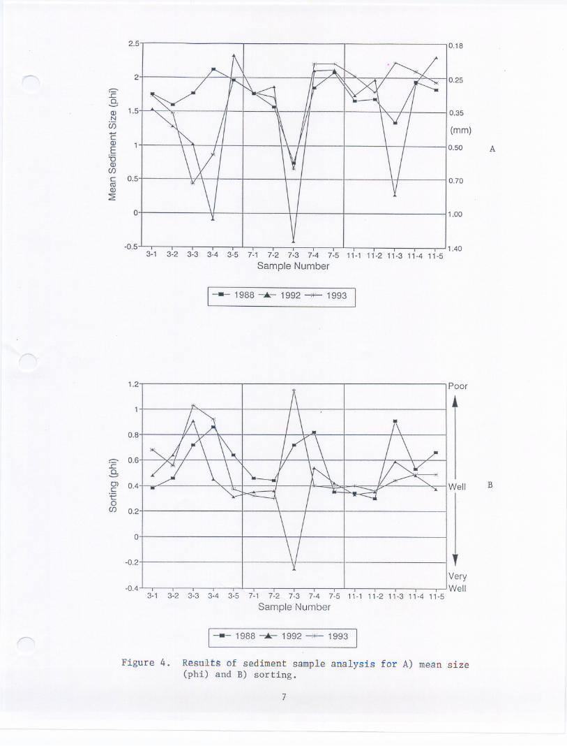
Figures 4A and 4B (Folk, 1980) are the plots for mean grain size (in phiunits and mm) and sorting (in phi units) of the sand fraction. The samplestaken at the toe of the beach (TOE) are consistently the coarsest materialalong the beach. The TOE zone usually is a very narrow step along the shoreand is not very representative of the entire profile. Another noticeabletrend is the relatively finer and more uniform sand sizes along profile 11 inApril, 1993 compared to profiles 3 and 7. This may be due to the lack ofbeach width in that area as a result of wave reflection from the exposedbulkhead. Except for that, the overall sand size distribution is finer at thebase of the dune and nearshore and coarser along the beach berm, high waterline and TOE. This is typical of estuarine beaches in the Chesapeake Bay(Hardaway et ai., 1991)
The sorting of sediments can be defined as the Inclusive GraphicStandard Deviation (Folk, 1980). The spread of the grain size distributionabout the mean defines the concept of sorting. Well sorted sands will have afrequency distribution curve that is sharp peaked and narrow; this means onlya few size classes are present (Friedman and Sanders, 1978). Poorly sortedsediments are represented by most size classes in the sample.
Analyses of the Cape Charles sediments generally show better sortingwith time at profile 11 and poorer sorting at profile 3 with profile 7 beingin transition. This coincides with the fining of the sediment at profile 11and coarsening at profile 3. This trend may support a general southwardtransport of material with the coarse sands mixing with the fine sands at thesouth end of the public beach to produce a poorly sorted sediment profile.
6
0.18
..0.5 I I I I I I I I I I I I I I I I I 11.40
3-1 3-2 3-3 3-4 3-5 7-1 7-2 7-3 7-4 7-5 11-1 11-2 11-3 11-4 11-5
Sample Number
1 1988 ~ 1992 -+- 1993
-0.2
Very-0.4 I I I I I I I I I I I I I I I I I I IWel1
3-1 3-2 3-3 3-4 3-5 7-1 7-2 7-3 7-4 7-5 11-1 11-2 11-3 11-4 11-5
Sample Number
1 1988 ~ 1992 -+- 1993
Figure 4. Resuits of sediment sample analysis for A) mean size(phi) and B) sorting.
7
2.5
2........:c
Q) 1.5NU)+JCQ)E'5Q)
(f)c 0.5roQ)
0
0.25
0.35
(mm)
0.50 A
0.70
1.00
0.8
........ 0.6:cQ.
Well B'-"CJ) 0.4c:e0(f) 0.2
0
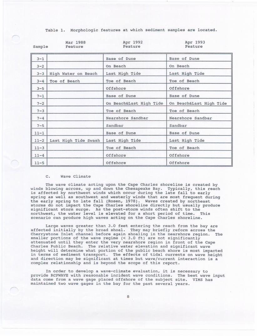
Table 1. Morphologic features at which sediment samples are located.
SampleMar 1988Feature
Apr 1992Feature
Apr 1993Feature
C. Wave Climate
The wave climate acting upon the Cape Charles shoreline is created bywinds blowing across, up and down the Chesapeake Bay. Typically, this reachis affected by northwest winds which occur during the late fall to earlyspring as well as southwest and westerly winds that are most frequent duringthe early spring to late fall (Rosen, 1978). Waves created by northeaststorms do not impact the Cape Charles shoreline directly but usually producesignificant storm surge. As the post-storm winds often shift to thenorthwest, the water level is elevated for a short period of time. Thisscenario can produce high waves acting on the Cape Charles shoreline.
Large waves greater than 3.0 feet entering the reach from the bay areaffected initially by the broad shoal. They may briefly reform across theCherrystone Inlet channel before again shoaling in the nearshore region. Thesmaller portions of the wave regime « 3.0 ft) are not significantlyattenuated until they enter the very nearshore region in front of the CapeCharles Public Beach. The relative water elevation and significant waveheight will determine what portion of the public beach shore is most impactedin terms of sediment transport. The effects of tidal currents on wave heightand direction may be significant at times but wave/current interaction is acomplex relationship and is beyond the scope of this report.
In order to develop a wave-climate evaluation, it is necessary toprovide RCPWAVE with reasonable incident wave conditions. The best wave inputdata come from a wave gage placed offshore of the subject site. VIMS hasmaintained two wave gages in the bay for the past several years.
8
3-1 Base of Dune Base of Dune
3-2 On Beach On Beach
3-3 High Water on Beach Last HiQh Tide Last HiQh Tide
3-4 Toe of Beach Toe of Beach Toe of Beach
3-5 Offshore Offshore
7-1 Base of Dune Base of Dune
7-2 On Beach&Last High Tide On Beach&Last High Tide
7-3 Toe of Beach Toe of Beach
7-4 Nearshore Sandbar Nearshore Sandbar
7-5 Sandbar Sandbar
11-1 Base of Dune Base of Dune
11-2 Last High Tide Swash Last High Tide Last High Tide
11-3 Toe of Beach Toe of Beach
11-4 Offshore Offshore
11-5 Offshore Offshore
Unfortunately, both deployments are on the west side of the bay and arepartially shielded from the northwest, west and southwest components of thewind/wave field to which Cape Charles is exposed. Therefore, it is necessaryto estimate the wave climate using available wind data. The nearestapplicable wind station is at Yorktown. Although it is on the opposite sideof the bay, the wind record is applicable to Cape charles, especially forwesterly winds of long duration (> 9 hrs).
The wave prediction model was initially developed by Sverdrup and Munk(1947) and revised by Bretschneider (1952, 1958). The current model (known as5MB) used in this study was further modified by Camfield (1977) and Kiley(1982). It is essentially a shallow water, estuarine, wind-wave predictionmodel.
Preliminary results from Hardaway and Milligan (in prep) show a closecorrelation between measured and predicted waves at the VIMS' Wolf Trap wavegage (Boon et al., 1992). This same wave prediction procedure, developedduring a previous project (Hardaway et al., 1991), was used to produce a setof wave conditions for input into RCPWAVE. The procedure involves thefollowing steps:
1. Determine effective fetch for three directions. This was
accomplished using procedures outlined in the U.S. Army Corps ofEngineers Shore Protection Manual (1977) for northwest, west andsouthwest directions from a point 10,500 feet due west of the CapeCharles public beach at -25 feet MLW. This also involvesmeasuring a bathymetric transect across the bay in each of thethree subject directions.
2. Use the above data as input into the 5MB program which provideswave height, period and length for a suite of wind speeds. Inthis case, wind speeds of 4 to 48 mph were used at 4 mphincrements. The results of this step are used to create a datafile of wind speeds and associated wave heights and periods foreach subject direction.
3. Wind data for four years, 1987 to 1990, were set up along with thedata file from step 2, as input requirements for running theprogram WINDOWS (Suh, 1990). WINDOWS takes the data file as inputparameters from step 2 and matches them with wind speed anddirection from each of the subject directions for each year toproduce another data file of wave heights, periods and directionsthrough a series of vector-averaging steps. The limitingcriterion is that the wind must be blowing from within theassigned sextant window for at least 9 hours. In other words,winds recorded by the wind station must be within, for example,300 and 3600 for 9 or more hours to qualify for this analysis.
4. The result of step 3 is a file for each year giving date, hourbeginning, wave height, wave period, local wave direction andduration of each qualifying wind event. These data then are meanweighted to provide a weighted mean for wave height, period anddirection with duration as the independent variable for each year(Table 2).
5. Finally, the results of step 4 were mean weighted for each year toproduce a weighted mean of wave parameters for the northwest, westand southwest directions (Table 3). The duration of each year wasaveraged for each direction. These results were used as inputinto RCPWAVE for annual conditions. One severe northwest stormcondition was also modelled. The RCPWAVE analysis will bediscussed further in section IV.
9
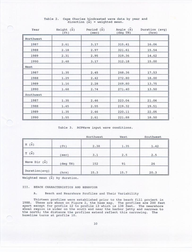
Table 2. Cape Charles hindcasted wave data by year anddirection (x) = weighted mean.
Year Height (x)
(ft)Period (x)
(see)Angle (x)(deg TN)
Duration (avg)(hrs)
Table 3. RCPWave input wave conditions.
Northwest West Southwest
Weighted mean (x) by duration.
III. BEACH CHARACTERISTICS AND BEHAVIOR
A. Beach and Nearshore Profiles and Their Variability
Thirteen profiles were established prior to the beach fill project in1988. These are shown on Figure 2, the base map. The profiles are 200 feetapart except for profile 12 to profile 13 which is 138 feet. The nearshoreshoal region is wider on the south end near the harbor jetty and narrows tothe north; the distance the profiles extend reflect this narrowing. Thebaseline turns at profile 10.
10
Northwest
1987 2.61 3.17 315.41 16.06
1988 2.18 2.97 321.61 15.54
1989 2.31 2.95 319.36 14.62
1990 2.48 3.17 312.18 15.00
West
1987 1.35 2.45 268.36 17.53
1988 1.29 2.42 272.80 18.00
1989 1.16 2.28 26980 13.75
1990 1.68 2.74 271.40 13.50
Southwest
1987 1.35 2.46 223.04 21.06
1988 1.45 2.55 219.32 19.51
1989 1.35 2.46 220.11 22.05
1990 1.55 2.61 221.88 18.50
H (x)(ft) 2.38 1.35 1.42
T (x)(see) 3.1 2.5 2.5
Wave Dir (x)(deg TN) 152 91 26
Duration(avg)(hrs) 15.3 15.7 20.3
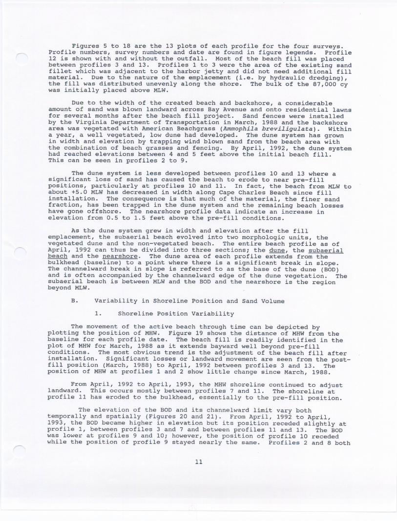
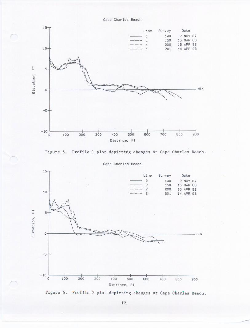
Figures 5 to 18 are the 13 plots of each profile for the four surveys.Profile numbers, survey numbers and date are found in figure legends. Profile12 is shown with and without the outfall. Most of the beach fill was placedbetween profiles 3 and 13. Profiles 1 to 3 were the area of the existing sandfillet which was adjacent to the harbor jetty and did not need additional fillmaterial. Due to the nature of the emplacement (i.e. by hydraulic dredging),the fill was distributed unevenly along the shore. The bulk of the 87,000 cywas initially placed above MLW.
Due to the width of the created beach and backshore, a considerableamount of sand was blown landward across Bay Avenue and onto residential lawnsfor several months after the beach fill project. Sand fences were installedby the Virginia Department of Transportation in March, 1988 and the backshorearea was vegetated with American Beachgrass (Ammophila breviligulata). Withina year, a well vegetated, low dune had developed. The dune system has grownin width and elevation by trapping wind blown sand from the beach area withthe combination of beach grasses and fencing. By April, 1992, the dune systemhad reached elevations between 4 and 5 feet above the initial beach fill.This can be seen in profiles 2 to 9.
The dune system is less developed between profiles 10 and 13 where asignificant loss of sand has caused the beach to erode to near pre-fillpositions, particularly at profiles 10 and 11. In fact, the beach from MLW toabout +5.0 MLW has decreased in width along Cape Charles Beach since fillinstallation. The consequence is that much of the material, the finer sandfraction, has been trapped in the dune system and the remaining beach losseshave gone offshore. The nearshore profile data indicate an increase inelevation from 0.5 to 1.5 feet above the pre-fill conditions.
As the dune system grew in width and elevation after the fillemplacement, the subaerial beach evolved into two morphologic units, thevegetated dune and the non-vegetated beach. The entire beach profile as ofApril, 1992 can thus be divided into three sections; the dune, the subaerialbeach and the nearshore. The dune area of each profile extends from thebulkhead (baseline) to a point where there is a significant break in slope.The channelward break in slope is referred to as the base of the dune (BOD)and is often accompanied by the channelward edge of the dune vegetation. Thesubaerial beach is between MLW and the BOD and the nearshore is the regionbeyond MLW.
B. Variability in Shoreline Position and Sand Volume
1. Shoreline Position Variability
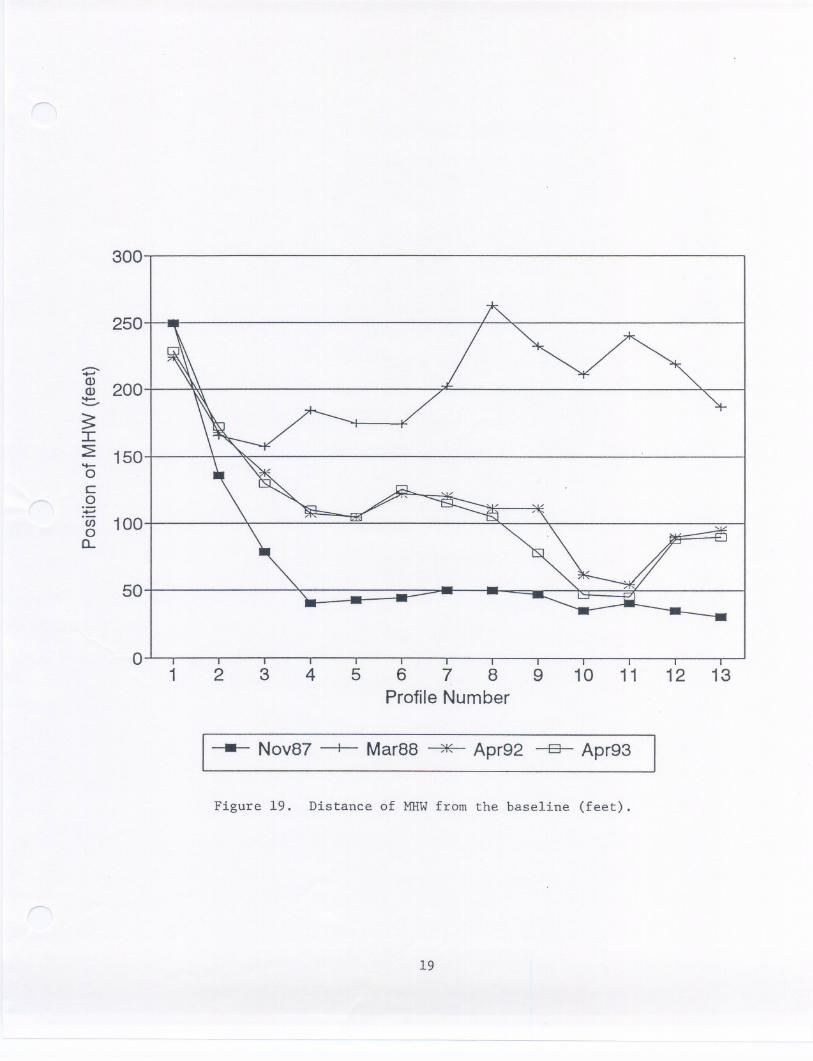
The movement of the active beach through time can be depicted byplotting the position of MHW. Figure 19 shows the distance of MHW from thebaseline for each profile date. The beach fill is readily identified in theplot of MHW for March, 1988 as it extends bayward well beyond pre-fillconditions. The most obvious trend is the adjustment of the beach fill afterinstallation. Significant losses or landward movement are seen from the post-fill position (March, 1988) to April, 1992 between profiles 3 and 13. Theposition of MHW at profiles 1 and 2 show little change since March, 1988.
From April, 1992 to April, 1993, the MHW shoreline continued to adjustlandward. This occurs mostly between profiles 7 and 11. The shoreline atprofile 11 has eroded to the bulkhead, essentially to the pre-fill position.
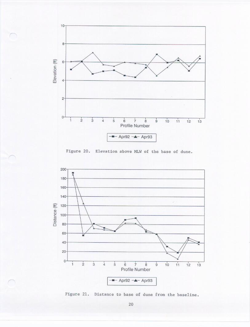
The elevation of the BOD and its channelward limit vary bothtemporally and spatially (Figures 20 and 21). From April, 1992 to April,1993, the BOD became higher in elevation but its position receded slightly atprofile 1, between profiles 3 and 7 and between profiles 11 and 13. The BODwas lower at profiles 9 and 10; however, the position of profile 10 recededwhile the position of profile 9 stayed nearly the same. Profiles 2 and 8 both
11
Cape Charles Beach
15
10
Line Survey1 1401 1501 2001 201
Date
2 NDV 8715 MAR8816 APR 9214 APR 93
-5
-10. 0 100 200 300 400 500 600 700 800 900
Distance. FT
Figure 5. Profile 1 plot depictiag changes at Cape Charles Beach.
Cape Charles Beach
15
10
5
HLW
co
.....
.....It)>OJ.....UJ
o
',.-
-5
-10o 100 200 300 400 500 600 700 800 900
Distance, FT
Figure 6. Profile 2 plot depicting changes at Cape Charles Beach.
12
,---
....5lL
C0..........It)>OJ 01
,-. "'" ...., "'"' HLW.....UJ
Line Survey Date2 140 2 NOV 872 150 15 MAR882 200 16 APR 922 201 14 APR 93
-5
-10o 100 200 300 400 500 600 700 800 900
Distance. FT
Figure 7. Profile 3 plot depicting changes at Cape Charles Beach.
Cape Charles Beach
15
-10o 100 200 300 400 500 600 700 800 900
Distance. FT
Figure 8. Profile 4 plot depicting changes at Cape Charles Beach.
13
--
Cape Charles Beach
15 .Line Survey Date
3 140 2 NOV873 150 15 MAR883 200 16 APR92
10+. .\ -..-..- 3 201 14 APR93/'N,\:/ \I. \ \
I-
5ri
11. ......\c:
. -\\0.....
\\ \...... .,ro\.\>_'>
(lJ o '-":::,...--:::=,--= --MLW
....W
Line Survey Date
4 140 2 NOV 874 150 15 MAR 884 200 16 APR 92
10+ [\. 4 201 14 APR 93
I-511.
c:
MLW
0...........ro>(lJ
0
.-..-..
....w
-5
co
.r1.....10>cu--UJ
HLWo
-5
-10o 100 200 300 400 500 600 700 800 900
Distance. FT
Figure 9. Profile 5 plot depi~ting changes at Cape Charles Beach.
Cape Charles Beach
15
10
l-LL. 5
HLW
c:o.r1.....10>cu--UJ
o"..-..--.-........
......~.- '-'-'--=:''::::.:--
-5
-10o 100 200 300 400 500 600 700 BOO 900
Distance. FT
Figure 10. Profile 6 plot depicting changes at Cape Charles Beach.
14
Cape Charles Beach
15.... Line Survey Date
5 140 2 NOV 875 150 15 MARBB5 200 16 APR 92
10-+- · -..-..- 5 201 14 APR 93
Line Survey Date
6 140 2 NOV B76 150 15 MARBB6 200 16 APR 926 201 14 APR 93
-5
-10o 100 200 300 400 500 600 700 BOO 900
Distance. FT
Figure 11. Profile 7 plot depicting changes at Cape Charles Beach.
Cape Charles Beach
15
l-LL 5
10
co........It)>QJ....UJ
o"--== "
.-0... ",.'
MLW
-5
-10o 100 200 300 400 500 600 700 800 900
Distance. FT
Figure 12. Profile 8 plot depicting changes at Cape Charles Beach.
15
Cape Charles Beach
15 , DateLine Survey7 140 2 NOY B77 150 15 MARBB7 200 16 APR 92
10+ -..-..- 7 201 14 APR93
Jt..,.I "
,. \"-I- 5 " \LL "\...c \--"0.... \\"....
\ \ .It) L.._ ">QJ o _._...... -' MLW.... "- '.
.. .. .. .. ",UJ
"\..
Line Survey DateB 140 2 NOY 878 150 15 MAR888 200 16 APR 92B 201 14 APR 93
15
10..
'\/,, "
./''j !\~-J \
':0-.. \
\ ""----\ '-.........\ \ ........--
'::: =.':':::: ::=..-..-.
I-U. 5
c:o....-<JfO>QJ.....UJ
o
-5
-10o 200 300100
Cape Charles Beach
400 500
.......",
600 700
MLW
800 900
Distance, FT
Figure 13. Profile 9 plot depicting changes at Cape Charles Beach.
15
10
I-U. 5
c:o....-<JfO>QJ.....UJ
o
-5
-10o 100 200 300
Cape Charles Beach
.'" -" ""-. ",
400 500
Line Survey10 14010 15010 20010 20 1
600 700
Date
2 NOV B715 MAR8816 APR 9214 APR 93
MLW
800 900
Distance. FT
Figure 14. Profile 10 plot depicting changes at Cape Charles Beach.
16
Line Survey Date
9 140 2 NOV 879 150 15 MAR889 200 16 APR 929 201 14 APR 93
15
10
I-U.
,:.\,
54A\.\ "' ~\ \
\,.\ '-~\ .,'~::-:..~ --
c:o.r1,CtJ>QJ-W
o' -.~.-
::-- -.. ..-" ., "'._e._ "
-5
-10o 100 200 300
Cape Charles Beach
400
Distance. FT
500
Line Survey11 14011 15011 20011 201
600 700
Date
2 NOV B715 MARB816 APR 9214 APR 93
HLW
800 900
Figure 15. Profile 11 plot depicting changes at Cape Charles Beach.
15
10
I-U. 5
c:o.....,
CtJ>QJ-W
o
-5
-10o 100 200 300
Cape Charles Beach
400 500
Line Survey12 14012 15012 20012 201
600 700
Date
2 NOV B715 MAR8816 APR 9214 APR 93
HLW
800 900
Distance. FT
Figure 16. Profile 12 plot depicting changes at Cape Charles Beachincluding the sewage outfall pipe.
17
-5
-10o 100 200 300 400 500 600 700 800 900
Distance. FT
Figure 17. Profile 12 plot depicting changes at Cape Charles Beach
excluding the sewage outfall pipe.
Cape Charles Beach
15
-5
-10o 100 200 300 400 500 600 700 800 900
Distance. FT
Figure 18. Profile 13 plot depicting changes at Cape Charles Beach.
18
Cape Charles Beach
15Line Survey Date
12 140 2 NOV B712 150 15 MARBB12 200 16 APR 92
10+ -...-....- 12 201 14 APR 93
I-U. 5
C0.........ro>OJ 01 , " " . ......... HLWw
Line Survey Date
13 140 2 NOV 8713 150 15 MAR8813 200 16 APR 92
10+ ------- 13 201 14 APR 93
I-U. 5
C0.........ro>OJ
01, --r..-. HLW...... '----- --------..... .....
w
300
o1 2 3 4 5 6 7 8 9
ProfileNumber10 11 12 13
--- Nov87 -+- Mar88 ~ Apr92 -a- Apr93
Figure 19. Distance of MHW from the baseline (feet).
19
250
Q)200Q)---
I
150-0c0;E
100(f)0a..
50
10
8
2
o2 3 4 5 6 7 8 9
Profile Number10 11 12 13
1-- Apr92-.- Apr93
Figure 20. Elevation above MLW of the base of dune.
2 3 4 56789
Profile Number10 11 12 13
1-- Apr92 -.- Apr93
Figure 21. Distance to base of dune from the baseline.
20
6'-"c0:.;:JCO>Q)ill 4
200
180
160
140
g 120Q)()
100cCO+--en
i:5 80
60
40
20
0
showed a slight increase in elevation. The BOD position of profile 2 grewsignificantly bayward whereas the BOD position of profile 8 moved only severalfeet. The average elevation of the BOD for both April, 1992 and April, 1993is about +5.0 feet MLW. This elevation was used to determine changes in dunevolume that will be discussed in the next section.
The peak elevation of the dune system has increased with time except forthe dune area between profiles 10 and 11, the area of chronic erosion.Between profiles 3 and 10, the peak dune elevations averaged +10 feet MLW byApril, 1993.
2. Beach, Dune, and Nearshore Volume Changes
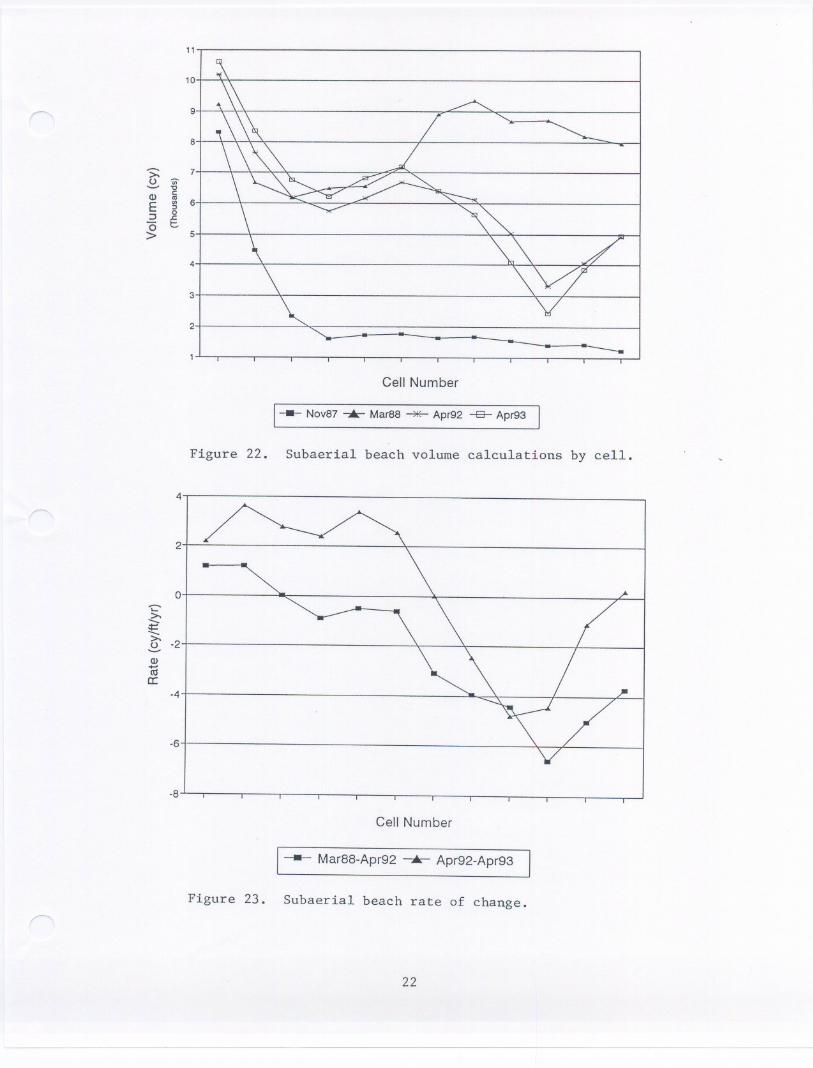
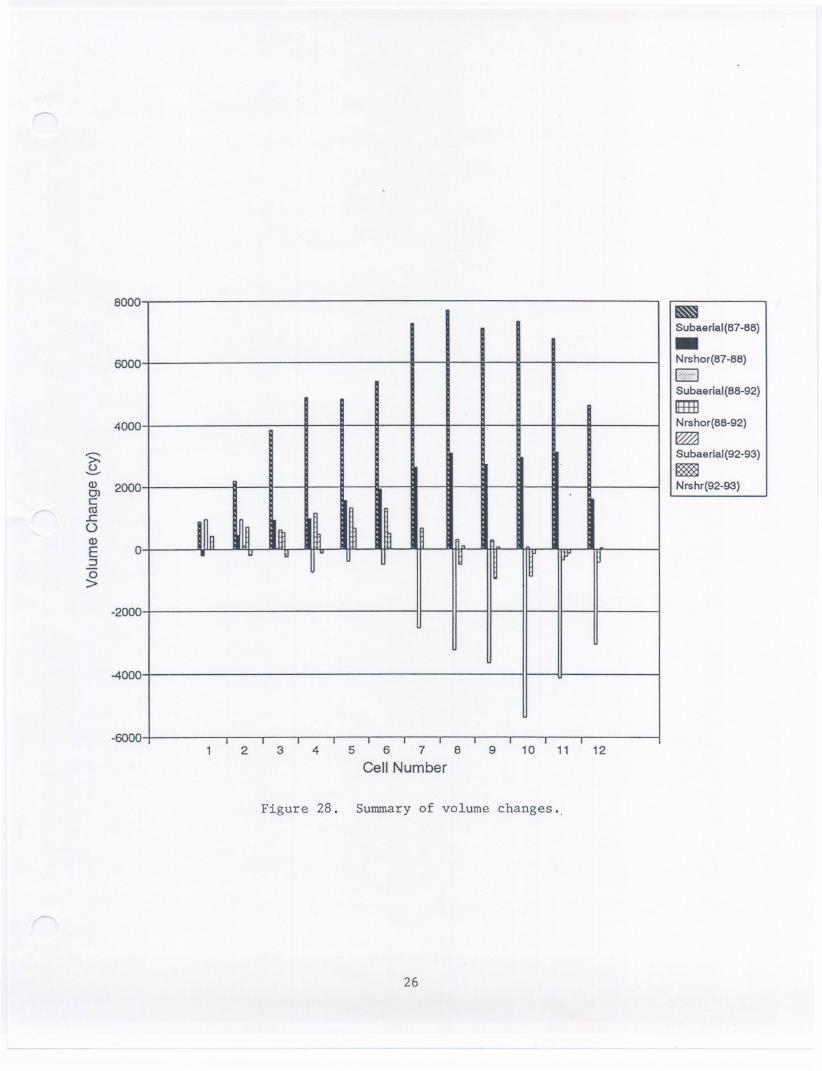
The amount of fill material either lost or gained along the shore zonecan be measured by changes in cubic yards (cy) per shore cell. The rate ofchange in fill volume is expressed in terms of cubic yards per linear footalong the shore per year (cyjftjyr). The subaerial portion of the beachprofile which includes the subaerial beach and dune has shown a marked loss ofmaterial since the beach nourishment project, from March, 1988 to April, 1993,in shore cells 6 through 12 (Figure 22). There has been an increase insubaerial volume in shore cells 1 to 3. There was an initial loss of materialbetween shore cells 3 and 6 from March, 1988 to April, 1992 but then asubsequent increase was seen from April, 1992 to April, 1993.
The rate of change of the subaerial portion of the profiles for the fouryears following the beach fill project show significant losses in cells 4 to12 (Figure 23). Slight gains in subaerial volume rates change occur in cells1 and 2 with no net gain at cell 3. From April, 1992 to April, 1993, lossrates continue for cells 8 to 11 with what would appear to be significantcorresponding gains in cells 1 to 6.
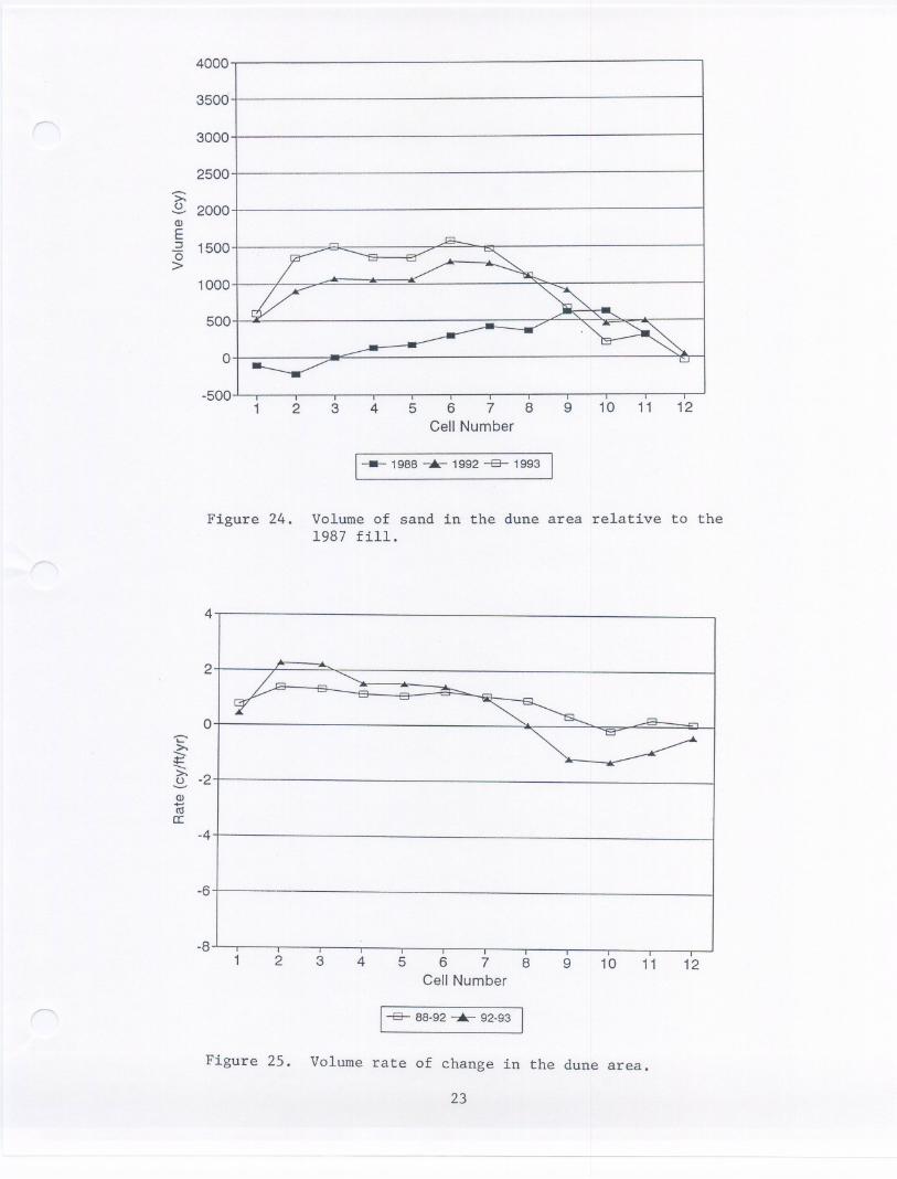
The dune portion of the subaerial region has shown a marked increase involume from March, 1988 to April, 1992 and to April, 1993 between shore cells1 and 8 (Figure 24). There was an increase in dune volume from March, 1988 toApril, 1992 from shore cells 8 to 13 but then the dune eroded significantly inthat area from April, 1992 to April, 1993. While small dunes still exist atprofiles 10 and 11, a portion of the beach between them has eroded such thatthe bulkhead is now exposed.
The rate or change of dune volume shows an increased rate of gain fromcells 2 to 5 and an increased rate of loss from cells 8 to 12 between the
periods March, 1988 to April, 1992 and April, 1992 to April, 1993,respectively (Figure 25). These patterns of rates of volume change correspondto the patterns of volume change for the subaerial region.
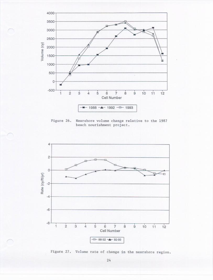
Generally, the nearshore region has experienced an increase in volumefrom March, 1988 to April, 1992 for shore cells 2 to 9 (Figure 26). Slightlosses in the nearshore have occurred in shore cells 10 to 13 from March, 1988to April, 1993 and cells 2 to 4 from April, 1992 to April, 1993. The rate ofvolume change in the nearshore for the first four years after the fill (March,1988 to April, 1992) reflect the volume change discussed above (Figure 27).
An increase in nearshore sediment volume creates a correspondingdecrease in nearshore water depth off the southern half of the public beachcreating a large low tide terrace. In fact, MLW moved an average of 95 feetbayward of its post-fill position by April, 1993 (profiles 1 to 7). Acorresponding landward movement of MLW was measured along the northern half ofthe public beach (profiles 8 to 13).
The overall assessment of the sediment volume changes at Cape Charles isthat the beach fill placed in March, 1988 has significantly eroded on thenorthern half of the project. The transport of the eroded material appears tobe southward alongshore as well as offshore. Also, a significant portion ofmaterial has been trapped in the dune area. A summary of volume changes is
21
Cell Number
--- Nov8? Mar88 """'*"" Apr92 -e- Apr93
Figure 22. Subaerial beach volume calculations by cell.
4
2
-6
-8
Cell Number
-- Mar88-Apr92 Apr92-Apr93
Figure 23. Subaerial beach rate of change.
22
- --
11
10
9
e
7.."to
(l) f;j
E CII 6:>:J 0
(5 E.> 5
4
3
2
0-C-<:-
>.-2
(l)-«Ic:-4
2 3 4 5 6 7 8Cell Number
9 10 11 12
1___ 1988 1992-B- 1993
Figure 24. Volume of sand in the dune area relative to the1987 fill.
-6
-82 3 4 5 6 7 8
Cell Number
9 10 11 12
1-8- 88-92 92-93
Figure 25. Volume rate of change in the dune area.
23
4000
3500
3000
2500
2000Q)E:J 1500"0>
1000
500
0
-5001
4
2
0'C'>-
-2Q)itta:
-4
1- 1988 1992-E3- 1993
Figure 26. Nearshore volume change relative to the 1987
beach nourishment project.
4000
3500
3000
2500
>:2000
Q)E:J 1500"5>
1000
500
0
-5001 2 3 4 5 6 7 8 9 10 11 12
CellNumber
4
2
0-.....
>.--
:E:.>.
-2
Q)..-coa:
-4
-6
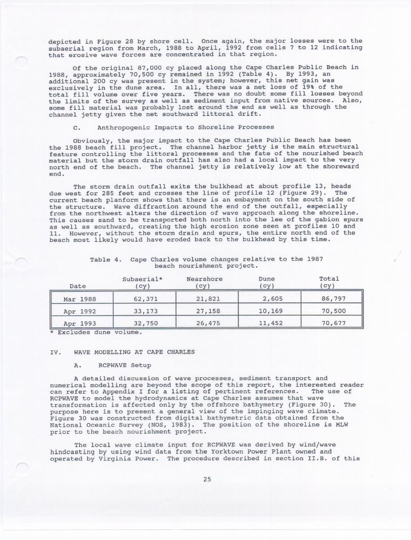
depicted in Figure 28 by shore cell. Once again, the major losses were to thesubaerial region from March, 1988 to April, 1992 from cells 7 to 12 indicatingthat erosive wave forces are concentrated in that region.
Of the original 87,000 cy placed along the Cape Charles Public Beach in1988, approximately 70,500 cy remained in 1992 (Table 4). By 1993, anadditional 200 cy was present in the system; however, this net gain wasexclusively in the dune area. In all, there was a net loss of 19% of thetotal fill volume over five years. There was no doubt some fill losses beyondthe limits of the survey as well as sediment input from native sources. Also,some fill material was probably lost around the end as well as through thechannel jetty given the net southward littoral drift.
C. Anthropogenic Impacts to Shoreline Processes
Obviously, the major impact to the Cape Charles Public Beach has beenthe 1988 beach fill project. The channel harbor jetty is the main structuralfeature controlling the littoral processes and the fate of the nourished beachmaterial but the storm drain outfall has also had a local impact to the verynorth end of the beach. The channel jetty is relatively low at the shorewardend.
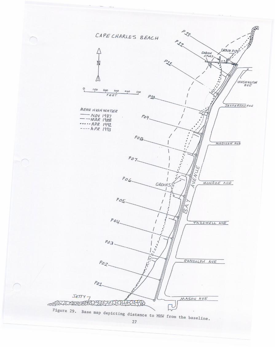
The storm drain outfall exits the bulkhead at about profile 13, headsdue west for 285 feet and crosses the line of profile 12 (Figure 29). Thecurrent beach planform shows that there is an embayment on the south side ofthe structure. Wave diffraction around the end of the outfall, especiallyfrom the northwest alters the direction of wave approach along the shoreline.This causes sand to be transported both north into the lee of the gab ion spursas well as southward, creating the high erosion zone seen at profiles 10 and11. However, without the storm drain and spurs, the entire north end of thebeach most likely would have eroded back to the bulkhead by this time.
Table 4. Cape Charles volume changes relative to the 1987beach nourishment project.
/
DateSubaerial*
(cy)
Nearshore
(cy)
Dune(cy)
Total(cy)
* Excludes dune volume.
IV. WAVE MODELLING AT CAPE CHARLES
A. RCPWAVE Setup
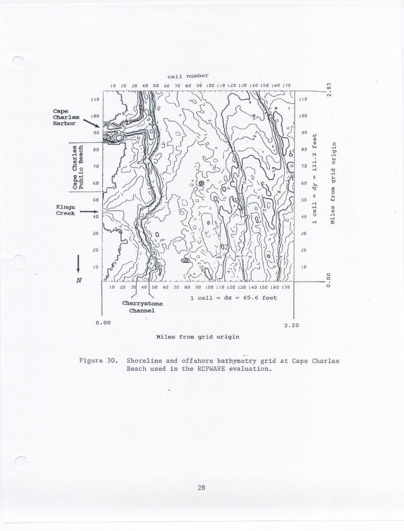
A detailed discussion of wave processes, sediment transport andnumerical modelling are beyond the scope of this report, the interested readercan refer to Appendix I for a listing of pertinent references. The use ofRCPWAVE to model the hydrodynamics at Cape Charles ass~mes that wavetransformation is affected only by the offshore bathymetry (Figure 30). Thepurpose here is to present a general view of the impinging wave climate.Figure 30 was constructed from digital bathymetric data obtained from theNational Oceanic Survey (NOS, 1983). The position of the shoreline is MLWprior to the beach nourishment project.
The local wave climate input for RCPWAVE was derived by wind/wavehindcasting by using wind data from the Yorktown Power Plant owned andoperated by Virginia Power. The procedure described in section II.B. of this
25
. .. . ..
Mar 1988 62,371 21,821 2,605 86,797
Apr 1992 33,173 27,158 10,169 70,500
Apr 1993 32,750 26,475 11,452 70,677
-4000
-60001 2 3 4 567 8
Cell Number9 10 11 12
Figure 28. Summary of volume changes..
26
8000 . ..Subaerlal(67 -66)-
6000 I I I I I I I I Nrshor(67-66)EiliJSubae rial(66-92)1mB
4000 I - I I I I I I I I I I I Nrshor(66-92)
I m.....'(92-93)
().........Q) 2000
D Nrshr(92-93)0> ItCas.c0Q)E 0:J0>
-2000
-l €TTY
CAPE C J./A R..1.E:S 8 EA C-/-I
o lOb UIo k:>o "= $DOL I . I . I
FEEl
MEAN HIGH WI'rTSR- NLJV /'l117- -MAR {'lEg., API? {q<jl
API? 199.3
MA7:J/~b7J Av
ASLHJ AVE__0-
Figure 29. Base map depicting distance to MEW from the baseline.27
cell number
10 cO JO 40 50 bO 70 80 90 100 J 10 120 IJO 140 150 IbO 1"10
CapeCharlesHArbor
!N
10 "/0 60 90 100 I!O 120 1:10 140 150 160 170
1 cell = dx = 65.6 feetCherrystone
Channel..
0.00
Hiles from grid origin
20
10
oo.o
2.20
Figure 30. Shoreline and offshore bathymetry grid at Cape CharlesBeach used in the RCPWAVEevaluation.
28
- ---
Mco.N
110
100
90.j.JQIQI I:
80'1-1 ..-j
N ..-j. J..IM 0
70 MM '0
..-jII J..I
60 >,'0 a
0II J..I
50 '1-1.-i.-i !IIQI QI
40 U M..-j
M :c
JO
report produces a significant wave height and period for three fetchexposures, Northwest (NW), West (W) and Southwest (SW), for the wind recordyears 1987 to 1990 (Table 3). We have defined these parameters as theseasonal modal wave conditions and they were modelled at a still water levelof +2.5 feet MLW or about MHW. A severe winter storm condition was also runusing an incident wave condition of 4.9 feet from the northwest at a stillwater level of +4.9 feet MLW which has a return frequency of three years (Boonet al., 1978) associated with an extratropical storm event.
B. Wave Height Distribution and Wave Refraction
RCPWAVE takes an incident wave condition at the seaward boundary of the
grid and allows it to propagate shoreward across the nearshore bathymetry.Frictional dissipation due to bottom roughness is accounted for in thisanalysis and is relative in part to the mean sand size (0.25 mm). Waves alsotend to become smaller over shallower bathymetry and remain larger over deeperbathymetry. In general, waves break when the ratio of wave height to waterdepth equals 0.78 (Komar, 1976).
Upon entering shallow water, waves are subject to refraction, in whichthe direction of wave travel changes with decreasing depth of water in such away that wave crests tend to parallel the depth contours. Irregular bottomtopography can cause waves to be refracted in a complex way and producevariations in the wave height and energy along the coast (Komar, 1976).
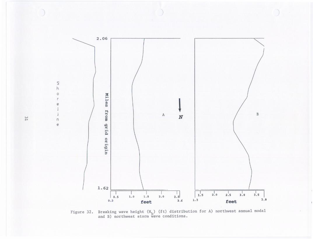
From the perspective of beach stability and behavior, it is the energyand momentum flux entering the surf zone that are important. Both quantitiesare proportional to the square of the wave height; the height of the setup atthe shore is directly proportional to the breaker wave height (Wright et al.,1987). However, in the case of the three annual modal wave conditions,RCPWAVE did not define a breaking wave condition across the grid's nearshoreregion due to the extreme dissipative nature of the shallow bathymetry. Thatis to say, the incident waves simply became gradually smaller over a longshallow nearshore region and only broke at the immediate shore cell. The waveheight and direction at the shore cell were then used to compute longshoretransport rates. Figures 31A and 318 show wave height distribution along theCape Charles shoreline for the southwest and west annual modal waveconditions. Figures 32A and 328 show the annual modal and storm wave for thenorthwest condition which defined breaking waves 1 to 3 cells from theshoreline.
The distribution of wave heights along the Cape Charles shoreline ispredicted to be rather uniform under the west modal condition. There arelarger waves predicted in the central portion of Cape Charles relative to thenorth and south ends under the southwest modal wave. Under the northwestmodal wave condition, slightly larger waves are predicted at each end of thepublic beach. The northwest storm condition shows a significant increase inbreaker wave height overall, especially at either end of the public beach.
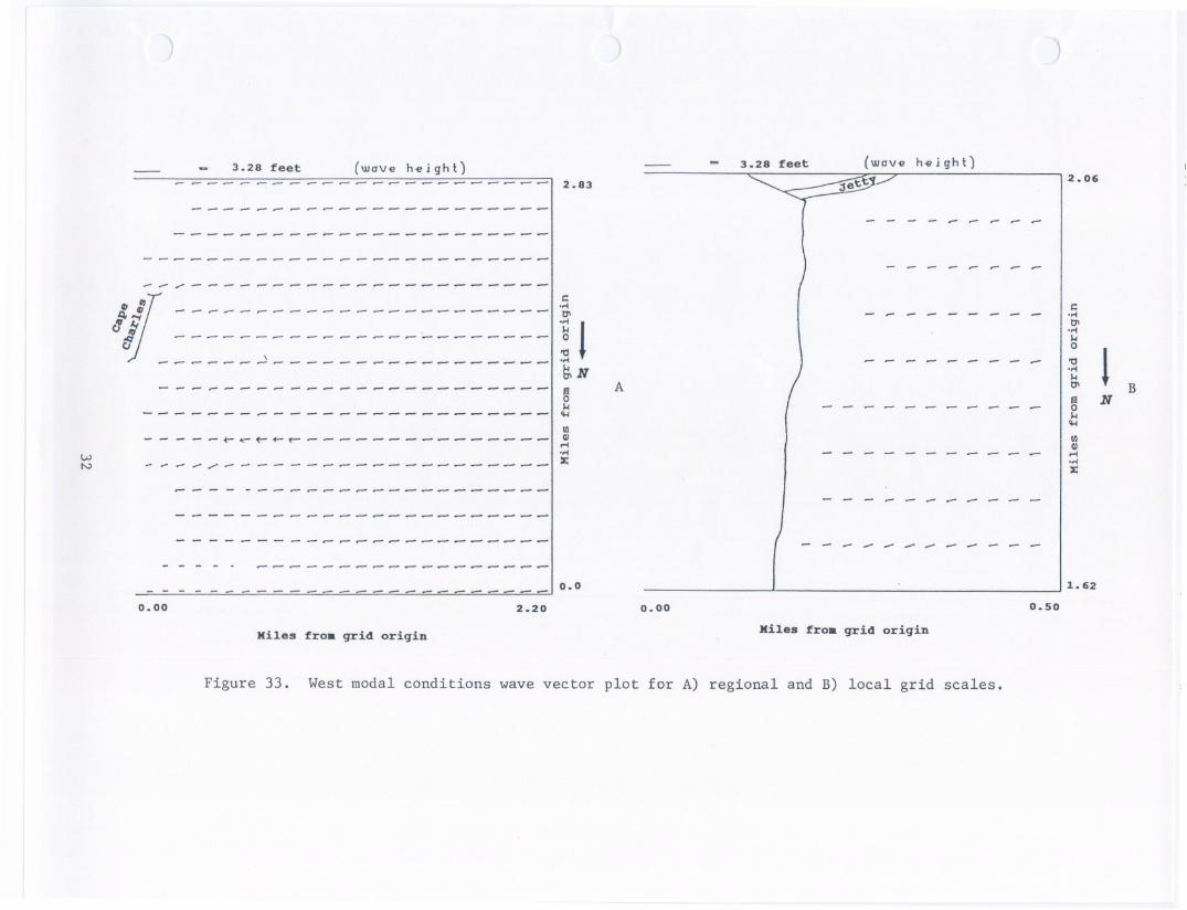
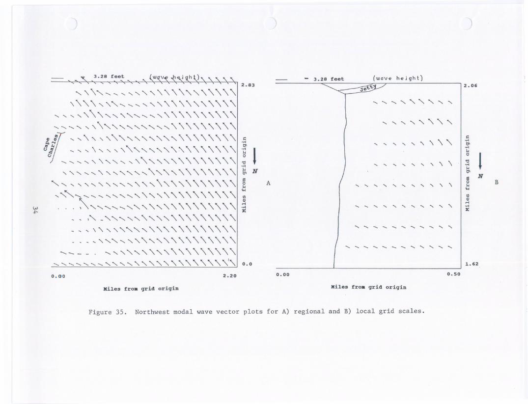
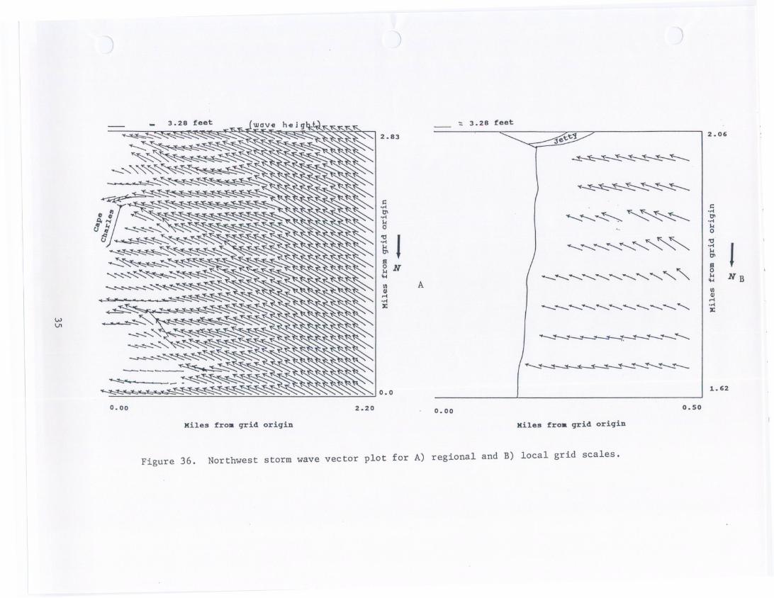
In order to compare the model runs for the modal wave conditions, waverefraction patterns were plotted from the RCPWAVE output. Figures 33, 34 and35 show the wave refraction vectors for the regional grid and the local gridfor each annual modal wave condition. Figure 36 depicts wave refractionvectors for the northwest storm condition. The waves break just beyond theshoreline in the nearshore region under the storm scenario.
The wave vector plot of the west modal condition shows little refractionor alteration in the wave patterns on the regional and local grid scales(Figures 33A and 338). The angle to the shoreline is slight or almost shorenormal. The west condition has a relatively low incident wave energy withabout the same event average duration as the northwest modal condition (i.e.about 15 hours).
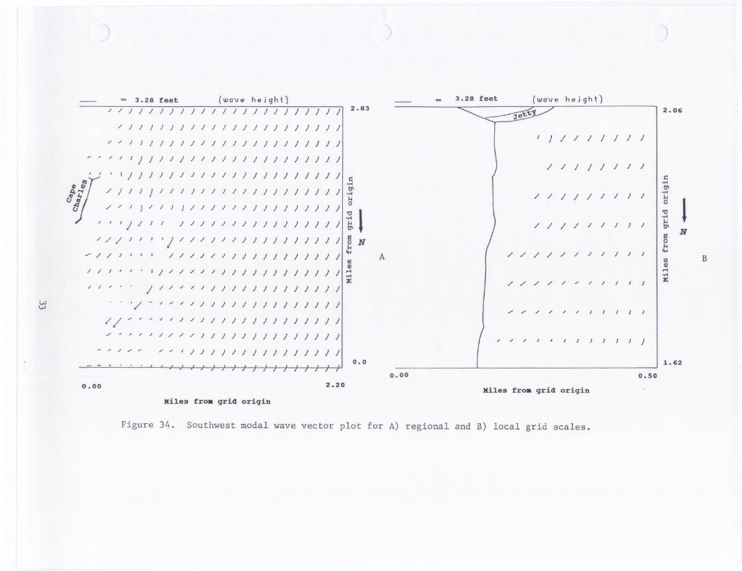
The southwest modal wave condition shows perhaps the most oblique waveapproach to the Cape Charles shoreline (Figures 34A and 348). This would bevery conducive to alongshore transport of beach material northward. However,
29 '
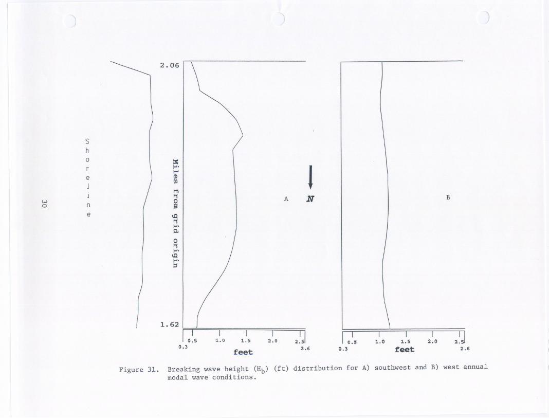
2.06
Figure 31. Breaking wave height (Hb) (ft) distribution for A) southwest and B) west annualmodal wave conditions.
Sh0
)
:J:r 1-'.
\!
I-'e (D
J!II
HI
\..VIi N I
0 n (A I B
e
1-'.Q.
0Ii1-'.
1-'.::1
2.06
feet
Figure 32. Breaking wave height (Hb) (ft) distribution for A) northwest annual modaland B) northwest storm wave conditions.
Sh0 tI:r .
\
1e (I)
j!IIHI
J 11 A I / Bw Nt-' n
e.
j;1,011.
.::s
3.28 feet (wave height)
0
("
B'~(j 1/1
C
WN
-----
- ---
---
,.,j-
~..-~+-(-
-....
-----
---------------
---------
----- -------------------------
-----------------
------------------------
----------------------
------------------
-------------
0.00 2.20
Hiles fro. grid origin
Figure 33.
2.83
0.0
hilight)3.28 feet
- - ---------
---------
-------
-.,.-..------
..- ..- ..- .". -- ..-
0.00
Hiles fro. grid origin
West modal conditions wave vector plot for A) regional and B) local grid scales.
0.50
2.06
c0'"tII0'"1-1ooa0'"1-1tII
§1-1....!IIQJ~0'"x
t BN
1.62
c0'"tII
o JN
§A
1-1....
!IIQJ
0'":t
- 3.28 feet (wave height) - - 3.28 feet (wave height)
/ / I I I I I I I I I I I I I I I } } } } } }I 2.83 -.......... ---<<3 ./ I 2.06
,/ I I J I I } I I I I I I I I } } } } } } }
J I I } I / I I I I } } } } } } } } } }II
J J / / I I I } }/ '" I
,/ ,'JIII/IIIIII}}}}}}/}}
/ / } I / / I I
, I' III/I/IIIIII}II}IIIII} c: c:..-4
3.( / / I I J I I I I I I I I I I / / / / / / / /
..-4C\C\..-4..-4 / / I / / I I / IQf; 0
!;''''I)/IJ}/IIIIII}I}}III}
0
!
'tI'.-4
"I//IIIIIIIIII}}}III}1 / / / / / I I J JN
Na
/// I I I'1/ 1/ I I I I I I}} I I I I} 0
....I ....
A ;' ;' / / ;' I I I J I I"" ;' / I I I/ / / / / I I I I I I I I I I I I
VI BVI
QIQI/ I I , ,/
I } ,/ / ,/ I I I I I I } I } I I I I II....c
..-4
:c ;' ;' ,/ ,/ ,/ '" ,/ I :c,/ I , I I ,/ '" ,/ I I I I I I I / / I } } } }'
VJ'/ - ,/ '" '" ,/ I / I I I / I I I } I I } IVJ
I ,./ -" " " ,/ ,
/ / -- ,
,/
,/ ,/ I ,/ I / I I I I I I I I I I } }
-" ,, ,/ ,/ I ,/ ,/ ,/ I I I I I I I I I I I I I }
I I
,/ '" ,/ , I I J J J 1 J I'" .- - '" '"
, / I I I I I } I I } } I I I }0.0
I I 1.62
0.00 0.50
0.00 2.20Hiles fro. grid oriqin
Hiles fro. grid oriqin
Figure 34. Southwest modal wave vector plot for A) regional and B) local grid scales.
!XI
--.12;
NIII0
III.
U1D1O
P1D
mOJ
sat1H
.N
...
011\
I/
//"
"/
1I
I1
//
,-/'
I1
I
//
/"/'
/1
II
//
/,-
II
II
.,-.
tI)-
GJ
.s::/
//
,-,-
II
I......
CO
III.
11
,-I
II
II
j:I0
'I'...
tI).s::
IC
I/
II
II
I1
..."t:I
'I'...
....::>
/I
II
II
1I
01-1
tJoa
bO:I
II
II
I1
Ior4
......III
I/
II
00I
II
1...
......IW
Ir"
III!X
I
v
GI
...c"t:I
...IIII::III
......IIII::0'MbOG
J1-1
0r"
0<
.01-10
<4-1tI)
......12;
1'10
CO
0......
.U1D1O
P1D
mOJ
sat1H
.Po
N0
01-1
,/,/,/,/,/,/,/,/,/,/,/,/,/,/,//
0N
,/,/,/,/,/,/,/,/,/,/,/,/,/,/,//
.0
NG
J,/,/,/,////,/,/,/,/,/,/,/,//
:>
,//////////////,//
GJ
//////////,/,/,/,/,//
:>
////,////,/,/,/,/,/,/,//
......///////,/,////////
III
,/./////././/.///////
"t:I
.0
////
/./
////.//////
13
CI
./././
1///////
/////
......
tI)
./
/1
1/
///,/
//
/.//
//
0GJ
//
II
/1//
//
//
//
.//
oa
]or4
/1
1I
///
1/
.//
/1.//
/1-1
01
II
1/
//
1/
/I
/I
//
/z
III
I//
1/
1I
/11
1/
1...
IW
.
tII
/I/
/II
11
1/
/I
/1
Lf"I
1/1///11
III
C""I
11
II
/I
I1
41
...c
CO
1/1//11/
/II
//
11
1...
GJ
III
1-1
1//'/////
/I
/I
//
I=
'bO
1'1//,/'///"/1
II
//
"I
I'M
////
./I
II
/
j/,
,I
//,/
I1
II
I1
/,
II
JI
/I
1I
/I
/;
II
II
II
//
II
00I
/8G
l"...I
I.0
Gcf
11:>":>
34
3.28 feet ':.3.28 feet
2.83
0.0 1.62
0.00 2.20 0.00 0.50
xiles fro. grid oriqin Xiles from grid oriqin
Figure 36. Northwest storm wave vector plot for A) regional and B) local grid scales.
r::....t7I.......0
liii
NfI.I
!II AQ)
....:c---- -----":::"::: RRRR"" Iw
\J1
2.06
I--------"'----"'--
r::"" "'---.. ....t7I.......0
<......-..............."" ""'" IJ
--..................................................................................................," I NB!IIQ)
----...................................-.....-.....-.....-.................."-. ....:c
""---"':--<......
------------"'--
the southwester usually occurs during periods of normal water levels and has alow incident wave condition close to that of the west modal wave condition
(i.e. about 1.3 feet). Also, RCPWAVE does not account for the effects of theharbor jetty that no doubt alters wave approach from the southwest bydiffraction. The general effect would be to cause southwest approaching wavesto bend and become more shore normal, thus reducing the potential foralongshore transport of beach material. The shallow nearshore created by thechannel jetty is considered in the RCPWAVE runs.
The northwest modal wave condition appears to most affected by theCherrystone Inlet Channel as seen in Figure 35A where the wave vectors becomemore southerly in direction and slightly larger in wave height. The northwestmodal wave begins more oblique to the grid shore than the southwest modal wavebut after crossing the channel and nearshore the resultant shore vectors aremore shore normal. The wave heights at the shoreline (Figure 358) are onlyslightly higher than the southwest and west conditions indicating that bottomfriction may affect the larger waves before they reach the shore cell.
The effect of one storm can translate into a major sediment transportevent that may be greater than several years of modal wave activity. Thesevere storm that is modelled in Figures 36A and 368 occurred in February,1987, just before the beach fill project. Several other slightly smallernorthwest wind events are recorded in the winters of 1988 and 1989. The stormcondition was run at an elevated water level which allows waves in the shore
zone to reach almost a meter in height before breaking. This will have amajor impact on the subaerial beach and dunes.
C. Littoral Transport Patterns
The movement of sand along a beach zone is dependent on breaking waveheight and angle of wave approach. Applications of littoral drift formulaeare subject to large errors; hence, the absolute magnitudes predicted must beconsidered suspect or, at best, accepted with caution (Wright at al., 1987).However, the relative magnitudes as they vary along the coast under differentwave scenarios is probably more meaningful as are predicted directions oftransport. Estimates obtained using the selected method in this reportinclude the moderating effects of breaker height variations.
The methods of calculating littoral drift used here are Gourlay's (1982)as discussed in Wright et al. (1987). The reader is referred once again toWright et al. (1987) for a complete discussion of these formulae and theirapplications. Erosional or accretionary changes in the volume of sand storedin a beach are determined by the gradients in alongshore flux (dQ/dy).Specifically, when the rate of littoral drift entering a given coastal sectorexceeds the rate exiting the sector, accretion results. Erosion results whenoutput exceeds input; there is no change when input and output are equal(Wright et al., 1987). Onshore-offshore sediment fluxes are not accounted forin the estimates of (dQ/dy) here.
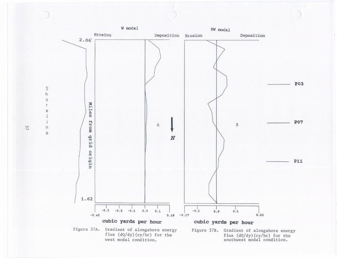
For the west and southwest modal wave conditions, the calculation of(dQ/dy) for the Cape Charles public beach are shown in Figures 37A and 378respectively. The calculation of (dQ/dy) for the west modal condition showsthat a significant area of deposition arises only near the channel jetty. Therest of the beach shows no net gain or loss (Figure 37A). For the southwestmodal wave condition, the plot of (dQ/dy) shows deposition along much of theCape Charles shore except for the area between profiles 4 and 7 and betweenprofile 11 to the northern boundary of the plot (Figure 378).
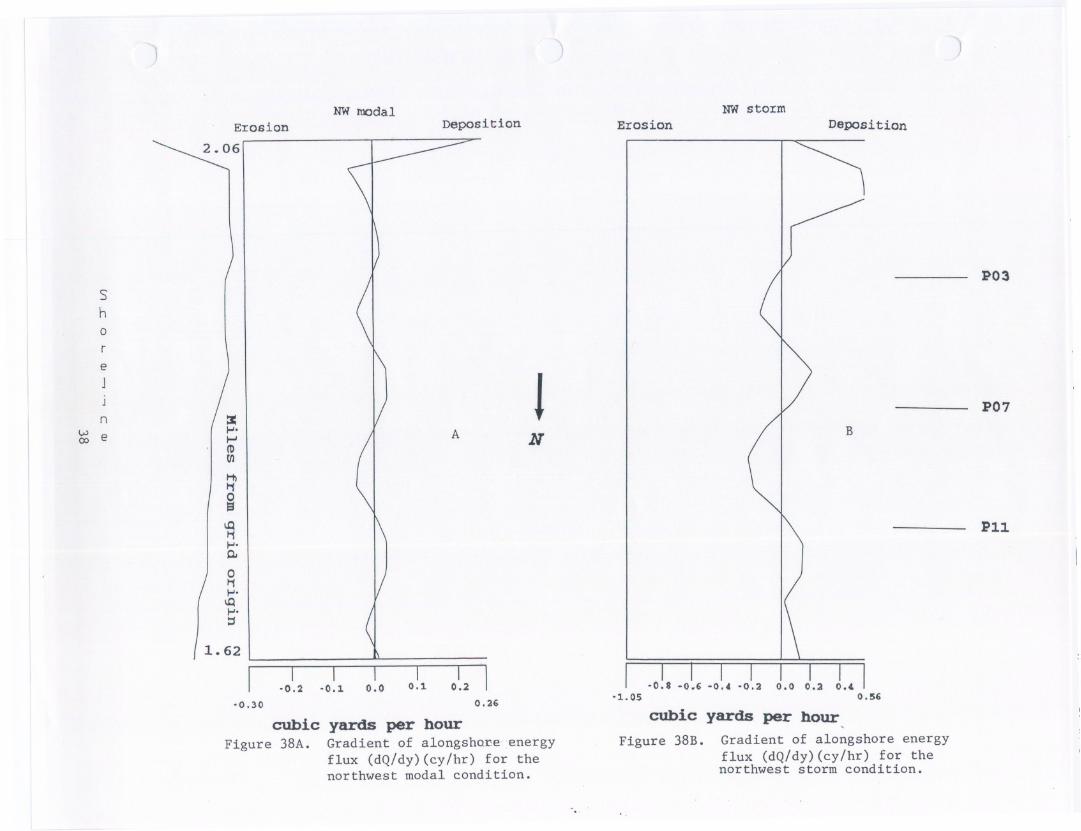
For the northwest modal wave condition, the plotted patterns of (dQ/dy)(Figure 38A) display alternating areas of erosion and deposition with asignificant depositional spike near the channel jetty. Predicted areas oferosion occur just north of that spike at profile 1 as well as near profiles 4and 9, and north of profile 13. According to the northwest storm condition,the patterns of erosion and deposition show erosion at profiles 4 and 9 andsignificant deposition near the channel jetty (Figure 388).
36
W JOOdal SW modalErosion
2 . 06'Deposition Erosion Deposition
1.62
I I I I I I I-0.3 -0.2 -0.1 0.0 0.1-0.40 0.18
cubic yards per hour
Figure 37A. Gradient of alongshore energyflux (dQ/dy)(cy/hr) for thewest modal condition.
I I I I I-0.1 0.0 0.1
-0.17 0.22
cubic yards per hour
Figure 37B. Gradient of alongshore energyflux (dQ/dy)(cy/hr) for thesouthwest modal condition.
5P03
h0r :J:
....e I-J
JIn!J1
J HI
1IVJ n A \1 B PO,
'-Ie
N....
0....1.01 I I I'....
P:L:L='
NW modal
E:rosion Deposition
:J:....
...,
(D
fI1
HI1'1
~
~....
Q.
o1'1....
\Q
....
=
1.62
.0.30 0.36
N
cubic yards per hourFigure 38A. Gradient of alongshor.e energy
flux (dQ/dy)(cy/hr) for thenorthwest modal condition.
I
NW sto:rm
Erosion Deposition
P03
PO,
Pl1
cubic yards per hour
Figure 38B. Gradient of alongshore energyflux (dQ/dy)(cy/hr) for thenorthwest storm condition.
". "
Sh0r
e
1
Jn
w00 e
The southwest modal wave condition has a greater per event duration butthe northwest modal wave condition has a slightly higher wave energy inputalong the Cape Charles shore. The one area of predicted deposition is nearthe channel jetty. The rest of the public beach shore fluctuates under theimpinging modal wave conditions with no other dominant erosion or depositionalareas. The southwest and northwest appear to modify each other in thatrespect. However, the northwest storm condition forces the transport patternsin such a way that the areas of erosion and deposition closely align with theshore changes determined from the field survey data. The best correlation isthe erosional area predicted between profiles 7 and 11 and the accretionalarea at the channel jetty.
What RCPWAVE fails to dQ is account for the beach fill, the effects oftidal currents and predict onshore-offshore sediment movement. Losses due toeolian action is also beyond its capability. The model did predictsignificant areas of deposition near the channel jetty as well as provide asomewhat balanced sediment transport scenario under modal wave conditions.The predicted area of significant erosion under the storm condition was alsofairly accurate. However, without field surveys or other shoreline changedata, it would be unwise to rely on the model output alone for shorelinemanagement plans. With the field data and a close model correlation, one canbegin to develop an accurate picture of a given shoreline situation.
V. CONCLUSIONS
Cape Charles' public beach has been reduced in volume approximately 19%since the beach nourishment project of 1988. Added fill at the north end isneeded to maintain a wide recreational beach. However, some type of sandretaining device should be used to keep the sand from eroding. Additionalprojects consisting simply of beach fill will only serve to increase the beachand nearshore along the southern half of the public beach.
The pattern of sediment movement has been well documented by a series of13 beach profiles taken by VIMS personnel before (November, 1987) and after(March, 1988) beach nourishment and subsequently in April, 1992 and April,1993. The beach, dune and nearshore regions have been significantly reducedin size and volume in an area corresponding to profiles 9, 10 and 11 to apoint that the bulkhead is exposed.
Except for profiles 1 and 2, the entire post-beach fill shoreline hasreceded. Most of the sand losses from the subaerial beach have shown up inthe nearshore and newly created dune system. A relatively wide usablesubaerial non-vegetated beach zone occurs only along the southernmost half ofthe public beach (profiles 1 to 6).
The increase in sediment volume in the nearshore also decreases thewater depth, particularly along the south end of the public beach shore.may tend to impede swimming at low water. The best option is to use theend of the beach at those times where the nearshore is somewhat deeper.
Thisnorth
Model runs using RCPWAVE showchannel jetty. Significant erosionand northwest storms at profiles 9,significant erosion.
predicted deposition just north of theis predicted during periods of high water10 and 11, the area of measured
Part of this erosional pattern may be attributed to the storm wateroutfall, which redirects northwest impinging waves by diffraction. However,without the outfall even more of the northern part of the public beach mayhave eroded back to the bulkhead.
39
VI. RECOMMENDATIONS
In order to correct the erosional areas and provide a more usablesubaerial beach between the BOD and MLW at Cape Charles Public Beach, thefollowing is recommended:
1. Place an offshore breakwater(s) at the north end of the publicbeach so that it works in conjunction with the existing stormwater outfall. Breakwater(s) specifications and position aresubject to further analysis.
2. Place approximately 15,000 cy of select beach sand along the midto northern half of the public beach in the area of severeerosion. The placement and position of the breakwater(s) will bedesigned to accommodate the fill. The bulkhead will be protectedas well.
3. Raise the level of the channel jetty to above MHW at the shorewardend and place a small spur on the north side to prevent sandlosses to the south around and through the jetty.
4. The dune grasses will continue to colonize the backshore andmigrate bayward. A limit should be established along thebackshore so the grasses will not reduce usable subaerial beachbut still maintain the protection and integrity of the dune systemduring storms. Each fall, grasses that grow beyond theestablished line can be transplanted into bare areas of the dunes.
ACKNOWLEDGEMENTS
The authors thank Lee Hill, Woody Hobbs and Jerome Maa for theireditorial reviews. A special thanks to Beth Marshall for the reportpreparation and compilation.
40
VII. REFERENCES
Boon, J.D., C.S Welch, H.S. Chen, R.J. Lukens, C.S. Fang, and J.M. Zeigler,1978. A Storm Surge Study: Volume I. Storm Surge Height-FrequencyAnalysis and Model Prediction for Chesapeake Bay. Spec. Rept. 189 inApplied Mar. Sci. and Ocean Engineering, Virginia Institute of MarineScience, Gloucester Point, VA., 155 pp.
Boon, J.D., D.A. Hepworth, and F.H. Farmer, 1992. Chesapeake Bay Wave ClimateWolf Trap Wave Station, Report and Summary of Wave Observations.Virginia Institute of Marine Science Data Report No. 42.
Bretschneider, C.L., 1952. The Generation and Decay of Wind Waves in DeepWater. Transactions of the American Geophysical Union, v. 33, p. 381-389.
Bretschneider, C.L., 1958. Revisions in Wave Forecasting: Deep and ShallowWater. Proceedings Sixth Conf. on Coastal Engineering, ASCE, Council onWave Research.
Byrne, R.J. and G.L. Anderson, 1978. Shoreline Erosion in Tidewater Virginia.SRAMSOE No. 111, Virginia Institute of Marine Science, College ofWilliam and Mary, Gloucester Point, VA.
Camfield, F.E., 1977. A Method for Estimating Wind-Wave Growth and Decay inShallow Water with High Values of Bottom Friction. Coastal EngineeringTech. Aid No. 77-6, October, 1977. U.S. Army Corps of Engineers,Coastal Engineering Research Center, Vicksburg, MS, 34 pp.
Ebersole, B.A., M.A. Cialone, and M.D. Prater, 1986. RCPWAVE - A Linear WavePropagation Model for Engineering Use. U.S. Army Corps of EngineersRept. CERC-86-4, 260 pp.
Folk, R.L., 1980. Petrology of Sedimentary Rocks, Hemphill Publishing Co.,Austin, TX, 182 pp.
Friedman, G.M. and J.E. Sanders, 1978. Principles of Sedimentology, JohnWiley and Sons, New York, 792 pp.
Gourlay, M.R., 1982. Nonuniform Alongshore Currents and Sediment Transport -A One Dimensional Approach. civil Eng. Res. Rept. No. CE31, Dept. Civ.Eng., Univ. of Queensland.
Hardaway, C.S., G.R. Thomas, and J.H. Li, 1991. Chesapeake Bay ShorelineStudies: Headland Breakwaters and Pocket Beaches for Shoreline ErosionControl. Special report in Applied Marine Science and Ocean EngineeringNo. 313, Virginia Institute of Marine Science, The College of Williamand Mary, Gloucester Point, VA, 153 pp.
Kiley, K., 1982. A Shallow Water Wind Wave Prediction Program. Based on U.S.Army Corps of Engineers Program developed by CERC, Fort Belvoir, VA.
Komar, P.D., 1976. Beach Processes and Sedimentation. Prentice-Hall, Inc.,Englewood Cliffs, NJ, 429 pp.
National Oceanographic Survey, 1983. Hydrographic Data Base. NOAA/NationalGeophysical Data Center, Boulder, CO.
Rosen, P.S., 1976. The Morphology and Processes of the Virginia ChesapeakeBay Shoreline. Dissertation, Virginia Institute of Marine Science,College of William and Mary, Gloucester Point, VA.
Suh, K.D., 1990. Windows Program. Virginia Institute of Marine Science,College of William and Mary, Gloucester Point, VA.
41
Sverdrup, H.U. and W.H. Munk, 1947. Wind, Sea, and Swell: Theory ofRelations for Forecasting. u.S. Navy Hydrographic Office Publ. No. 601.
u.S. Army Corps of Engineers, 1977. Shore Protection Manual. CoastalEngineering Research Center, Fort Belvoir, VA.
u.S. Army Corps of Engineers, 1991. Emergency Shoreline Erosion Study, Townof Cape Charles, Northampton County, Virginia. Norfolk, VA, 41 pp.
Wright, L.D., C.S. Kim, C.S. Hardaway, Jr., S.M. Kimball, and M.O. Green,1987. Shoreface and Beach Dynamics of the Coastal Region from CapeHenry to False Cape, Virginia. Virginia Institute of Marine ScienceTechnical Report.
42
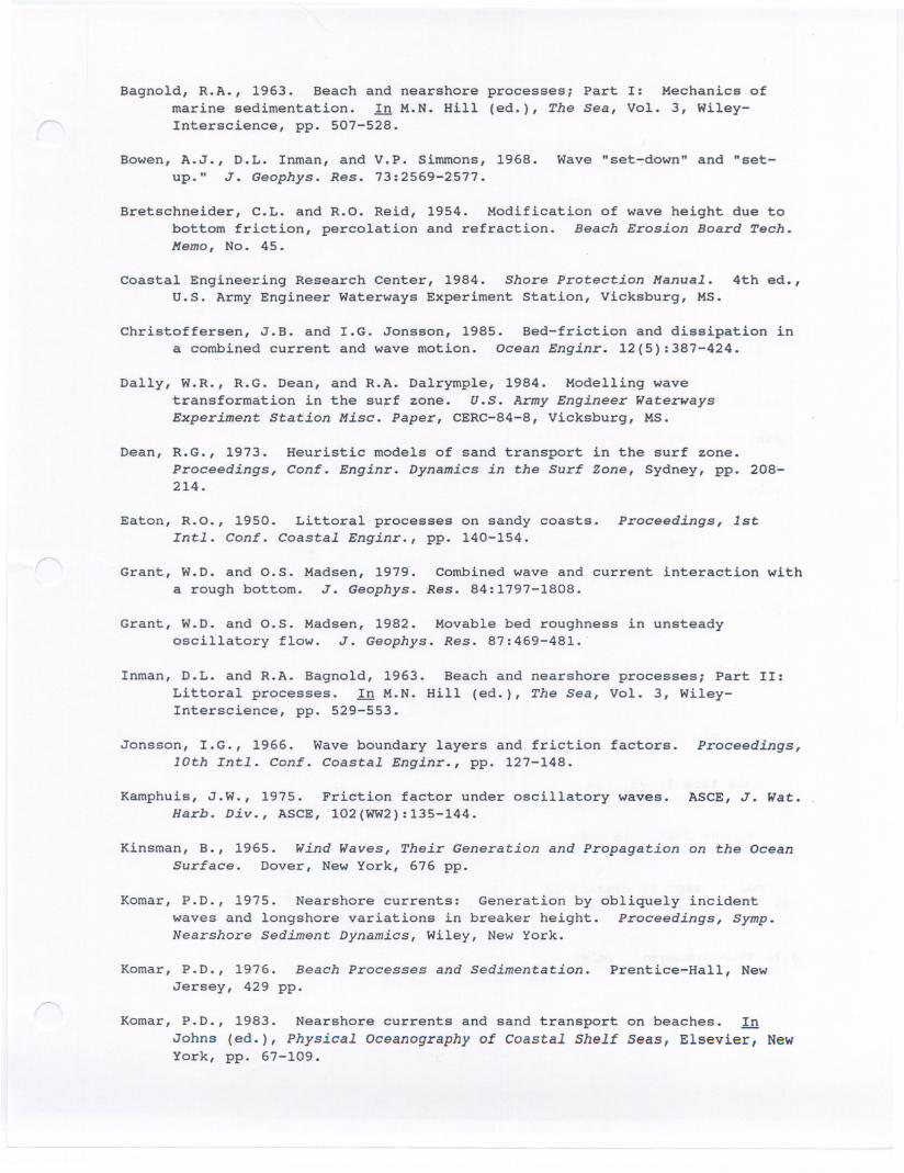
APPENDIX I
Additional References about Littoral Processes and Hydrodynamic Modeling
-
Bagnold, R.A., 1963. Beach and nearshoremarine sedimentation. In M.N. Hill
Interscience, pp. 507-528.
processes; Part I: Mechanics of(ed.), The Sea, Vol. 3, Wiley-
Bowen, A.J., D.L. Inman, and V.P. Simmons, 1968. Wave "set-down" and "set-up." J. Geophys. Res. 73:2569-2577.
Bretschneider, C.L. and R.O. Reid,
bottom friction, percolationMemo, No. 45.
1954. Modification of wave height due toand refraction. Beach Erosion Board Tech.
Coastal Engineering Research Center, 1984. Shore Protection Manual. 4th ed.,u.S. Army Engineer Waterways Experiment Station, Vicksburg, MS.
Christoffersen, J.B. and I.G. Jonsson, 1985. Bed-friction and dissipation ina combined current and wave motion. Ocean Enginr. 12(5):387-424.
Dally, W.R., R.G. Dean, and R.A. Dalrymple, 1984. Modelling wavetransformation in the surf zone. u.S. Army Engineer WaterwaysExperiment Station Misc. Paper, CERC-84-8, Vicksburg, MS.
Dean, R.G., 1973. Heuristic models of sand transport in the surf zone.
Proceedings, Conf. Enginr. Dynamics in the Surf Zone, Sydney, pp. 208-214.
Eaton, R.O., 1950. Littoral processes on sandy coasts. Proceedings, 1stIntI. Conf. Coastal Enginr., pp. 140-154.
Grant, W.D. and O.S. Madsen, 1979. Combined wave and current interaction witha rough bottom. J. Geophys. Res. 84:1797-1808.
Grant, W.D. and O.S. Madsen, 1982. Movable bed roughness in unsteadyoscillatory flow. J. Geophys. Res. 87:469-481."
Inman, D.L. and R.A. Bagnold, 1963. Beach andLittoral processes. In M.N. Hill (ed.),Interscience, pp. 529-553.
nearshore processes; Part II:
The Sea, Vol. 3, Wiley-
Jonsson, I.G., 1966. Wave boundary layers and friction factors. Proceedings,10th IntI. Conf. Coastal Enginr., pp. 127-148.
Kamphuis, J.W., 1975. Friction factor under oscillatory waves. ASCE, J. Wat.Barb. Div., ASCE, 102(WW2):135-144.
Kinsman, B., 1965. Wind Waves, Their Generation and Propagation on the OceanSurface. Dover, New York, 676 pp.
Komar, P.D., 1975. Nearshore currents: Generation by obliquely incidentwaves and longshore variations in breaker height. Proceedings, Symp.Nearshore Sediment Dynamics, Wiley, New York.
Komar, P.D., 1976. Beach Processes and Sedimentation. Prentice-Hall, NewJersey, 429 pp.
Komar, P.D., 1983. Nearshore currents and sand transportJohns (ed.), Physical Oceanography of Coastal ShelfYork, pp. 67-109.
on beaches. In
Seas, Elsevier, New
Komar, P.D. and D.L. Inman, 1970. Longshore sand transport on beaches. J.Geophys. Res. 73(30):5914-5927.
Kraus, N.C. and T.O. Sasaki, 1979. Effects of wave angle and lateral mixingon the longshore current. Coastal Enginr. in Japan 22:59-74.
LeMehaute, B. and A. Brebner, 1961. An introduction tolittoral processes. C.E. Research Report No. 14,Enginr., Queen's Univ., Kingston, ontario.
coastal morphology and
Dept. of civil
Longuet-Higgins,currents.
Transport,
M.S., 1972. Recent progress in the studyIn R.E. Meyer (ed.), Waves on Beaches andAcademic Press, New York, pp. 203-248.
of longshore
Resulting Sediment
Longuet-Higgins, M.S. and R.W. Stewart, 1962. Radiation stress and masstransport in gravity waves, with application to surf beats. J. FluidMech. 13:481-504.
Madsen, O.S., 1976. Wave climate of the continental margin: Elements of itsmathematical description. In D.J. stanley and D.J.P. Swift (eds.),Marine Sediment Transport and Environmental Management, Wiley, New York,pp. 65-90.
Munch-Peterson, J., 1938. Littoral drift formula. Beach Erosion Board Bull.4(4):1-31.
Nielsen, P., 1983.variation due
7(3):233-252.
Analytical determination of nearshore wave heightto refraction, shoaling and friction. Coastal Enginr.
Savage, R.P., 1962. Laboratory determination of littoral transport rates. J.WW and Harbours Div., ASCE 88(WW2):69-92.
Weggel, J.R., 1972. Maximum breaker height. J. WW and Harbours Div., ASCE
78(WW4):529-548.
Wright, L.D., 1981. Beach cut in relation to surf zone morphodynamics.Proceedings, 17th Inti. Conf. Coastal Enginr., Sydney, Australia, pp.978-996.
Wright, L.D. and A.D. Short, 1984. Morphodynamic variability of surf zonesand beaches: A synthesis. Mar. Geol. 56:93-118.
Wright, L.D., R.J. Guza, and A.D. Short, 1982. Dynamics of a high energydissipative surfzone. Mar. Geol. 45:41-62.
Wright, L.D., A.D. Short, and M.D. Green, 1985. Short-term changes in themorphodynamic states of beaches and surfzones: An empirical predictivemodel. Mar. Geol. 62:339-364.
Wright, L.D., P. Nielsen, N.C. Shi, and J.H. List, 1986b. Morphodynamics of abar-trough surfzone. Mar. Geol. 70:251-285.