1

Public Procurement and Non-contractible Quality: Evidence from

Elderly Care

Mats A. Bergman, Sofia Lundberg and Giancarlo Spagnolo

September 6, 2012

Abstract:

Many quality dimensions are hard to contract upon and are at risk of degradation

when the service is procured rather than produced in-house. On the other hand,

procurement may foster performance-improving innovation. We assemble a large

data set on elderly care services in Sweden for the 1990-2009 period, including

survival rates, our measure of non-contractible quality, and indicators of subjectively

perceived quality of service. We estimate the effects of municipalities’ decision to

procure rather than produce in-house on non-contractible quality using a difference-

in-difference approach and controlling for a number of other potential determinants.

The results indicate that procurement significantly increases non-contractible quality

as measured by survival rate, reduces the cost per resident but does not affect

subjectively perceived quality.

Keywords: incomplete contracts, privatization, procurement, quality, elderly care,

mortality, outsourcing, nursing home, performance measurement.

JEL code: H57, I18, L33

Financial support from the Swedish Research Council and the Swedish Competition Authority is

gratefully acknowledged. We would also like to thank seminar participants at Karlstad University,

Norway University of Science and Technology, the Swedish Competition Authority, Södertörn

University, Uppsala University, Umeå University, the 4th

IPPC in Seoul, EARIE in Istanbul, 29th

Arne Ryde Symposium in Lund and The Research Institute of Industrial Economics. Södertörn University; Umeå University; and University of Tor Vergata and SITE, respectively.

2

1. Introduction

Government and private firms outsource many activities to external providers. Public

procurement alone accounts for an estimated 15 percent of the world GDP (Bajari

and Lewis, 2011). Cost savings from increased specialization, scale economies and

supplier competition can be very large (Bandera, Prat and Valletti, 2009).

However, maintaining an appropriate quality level may be a concern. For

standardized products, quality degradation can be avoided by properly written and

managed contracts. The risk of quality degradation is higher, however, when the

procured products or services are complex and important quality dimensions are hard

to verify and contract upon. In this paper we attempt to empirically identify the

effects of shifting from in-house production to outside procurement on non-

contractible quality dimensions - both objectively measured and subjectively

perceived ones - for a common but rather hard-to-contract-upon publicly provided

service: elderly (nursing home) care.

Quality degradation in non-contractible dimensions after outsourcing can occur

because the cost-saving incentives of private contractors are much stronger than

those of public in-house providers, and cost savings tend to affect the provision of

quality (Hart et al., 1997).

Degradation of non-contractible quality can be particularly acute in public

procurement also for another reason. In private transactions, where buyers have

substantial discretion and can react to non-verifiable quality signals, reputation,

brand names and long-term informal relations are used to support high-quality

equilibrium sustained by the link between current performance and future sales

(Klein and Leffler, 1981; Macaulay, 1963).

Public procurement legislation instead requires procedures to be objective and

transparent for accountability reasons, limiting discretion and thereby the scope for

such mechanisms (Kelman, 1987). In many countries a public procurer is in principle

not allowed to discriminate in favour of strong brand names, nor of providers that

performed well in the past on non-verifiable performance dimensions.

Similarly, while a public procurement contract can give the buyer an option to extend

the duration of the supply contract, the exact length of the extension must typically

3

be specified in the original contract. Under many public procurement legislations the

criteria driving the decision to award the extension must be ‘objective’, that is,

verifiable. Even where a public procurer has the possibility of linking future sales to

provided quality, e.g., via vendor rating and contract renewal schemes, existing

regulations make this link very tenuous for non-contractible dimensions that cannot

be audited by third parties and therefore generate accountability concerns.

In this paper we study the effect of outside procurement on non-contractible quality

dimensions of publicly provided nursing home services in Sweden.1 To do this we

construct and study a panel including almost all Swedish municipalities over a period

of up to 19 years.

We consider two main measures for non-contractible quality. The first one is

mortality rates, a quality indicator commonly used in the literature and one that was

not contracted upon (probably because it is too noisy at the single institution level

and also so as not to induce screening of patients) and that is objectively measured

for the whole panel.

The second indicator is a customer satisfaction index, a measure of subjectively

perceived quality that was also not contracted upon but that is unfortunately only

available for a cross-section of municipalities. We argue that we can estimate at least

part of the effects of procurement, or outsourcing, on non-contractible quality via a

statistical analysis of the impact of procurement on mortality rates and customer

satisfaction indicators. In addition to this, we study the effect of procurement on the

cost for provision of nursing home care for the elderly.

Using a difference-in-difference random effects approach we find a significant

decrease in the mortality rates of the elderly after a regime shift from in-house

provision to (partial) outsourcing. The results are consistent with a 1-3 percent

decrease in mortality among residents of nursing-homes or, equivalently, with an

extension by about half a month of the expected remaining 1-1.5 years of life upon

entry.

1

In Sweden the public sector - including publicly held corporations that must adhere to the

Procurement Act - is estimated to procure each year for about SEK 500 billion (€ 50 billion),

corresponding to 16 to 18 percent of GDP (Bergman, 2008).

4

Procurement is associated with a 3 percent reduction of the per-resident cost of

service but there is no reduction of total cost, suggesting that there is a balancing

expansion of the number of beds. We find some indication of a negative impact of

procurement on subjectively perceived quality. While procuring municipalities do

not differ significantly from other municipalities, there is a significant negative

association between the share of homes outsourced in a municipality and customer

satisfaction.

The reminder of the paper unfolds as follows. Section 2 discusses prior empirical

research that can be related to the current study, as well as the theoretical

background. Section 3 describes the characteristics of the elderly-care industry in

Sweden followed by Section 4 that presents our database and reports some

descriptive statistics. Section 5 describes our empirical approach; Section 6 presents

our main results while Section 7 includes an extended empirical analysis where the

main results are checked for inclusion of trend specific effects, costs and admission

policy as well as to what degree the provision of nursing home care is procured.

Finally, Section 8 briefly concludes.

2. Theory and prior empirical studies

Theory

With pure in-house production, there is no element of competition. Then,

government may have a more direct control over the various quality dimensions of

the services that are offered. However, if quality cannot be contracted on, in-house

production may also suffer from poor quality. After all, government tasks must be

delegated to agents – employees – that tend to be self-interested.

The analysis of Hart et al. (1997) focuses precisely on how the mode of public goods

production – in-house by the government vs procured from private contractors –

affects non-contractible quality provision, as well as innovation and cost efficiency.

They propose an incomplete-contracts model where the producing agent can make

non-verifiable investments to increase (non-verifiable) quality or to reduce cost; the

latter investment will, however, be associated with a fall in quality.

The main presumed differences between internal and external production is that,

first, the government can veto any investment for in-house production but not for

5

outsourced production; and, second, that an in-house agent (a government employee)

will be given a smaller share of the rents created by these investments. The

implication is that an outside agent will be more prone to making both types of

investments – but will tend to invest too much in cost savings. If non-contractible

cost reductions have large deleterious effects on non-contractible quality and there is

little scope for efficiency-enhancing innovation, then in-house government

production may be preferred. Otherwise, outside procurement should be preferred as

it may lead to increased quality besides lower costs.

Abandoning the stark assumption that quality is completely non-contractible, Levin

and Tadelis (2010) assume that the cost of specifying and enforcing quality for

external provision varies across goods and services, and that it is convex in the

required quality level. Again, the government can opt for in-house provision. With

in-house production, contracting costs will be zero, but cost incentives will be

weaker, so production costs will be higher. The conclusion parallels that of Hart el

al. (1997): when quality is important enough, in-house production dominates

outsourcing. In Levin and Tadelis’ model, the reason is that saving on transaction

costs more than compensates for the decrease in productive efficiency.

Putting together the results of Hart et al. (1997) with political theories of

privatization emphasizing the political costs of publicly owned enterprises linked to

exchanges of overemployment against vote (e.g. Boycko et al., 1996), in his

influential survey Shleifer (1998) concludes that privatization dominates in-house

government production unless: “1) opportunities for cost reductions that lead to non-

contractible deterioration of quality are significant; 2) innovation is relatively

unimportant; 3) competition is weak and consumer choice is ineffective; and 4)

reputational mechanisms are also weak.”

Indeed, in standard market interaction the suppliers’ incentives to degrade quality are

checked by their concern over reputation and brand-name value, even in the absence

of repeat purchases (Bar-Isaac and Tadelis, 2008). With repeat purchases, buyers

may establish long-term supply relations, supported by threats to break those

relations if the suppliers degrade quality (MacLeod, 2007). In general, the main

mechanism to maintain a quality level above the minimum when quality is non-

6

verifiable and observable only ex post is to have future sales increasing in current

quality level.

In the context of public procurement, if quality is non-verifiable but observable in

advance, the procurement design could give the procurer sufficient discretion to

choose high-quality providers (Kelman, 1987). The disadvantage is of course that the

procurer will then be less accountable (Banfield, 1975). The outcome will not be

fully predictable and it will be impossible to verify ex post that the contract was

awarded to the supplier with the best bid, making the process susceptible to

corruption. Because of these concerns, public procurement rules generally limit the

freedom of the procurer to select provider on the basis of reputation or other non-

verifiable aspects. Hence, rules set up to deal with one problem (accountability) may

create another (adverse selection); one that would not exist in the absence of the

rules.

If quality is non-verifiable and observable only ex post, the situation is even more

difficult. The buyer must now give the seller incentives to provide quality. Bonuses

(monetary or in terms of contract renewal) or penalties that depend directly on ex-

post observed quality cannot help, unless the buyer can a) discretionally decide

bonuses and penalties and b) make it credible that it will fairly reward high quality

and punish low quality (Calzolari and Spagnolo, 2009; Iossa and Rey, 2010).

Although a public entity may conceivably be able to commit to such a scheme, it

may not be possible or desirable to give the procurer such discretion – due to the risk

of corruption.

Alternatively, an element of consumer choice may link current quality and future

sales also in a public procurement setting. This can be done without post-award

competition, as is typical of the procurement of public transport services. The

contract may be structured so that the seller retains the ticket revenues – and these

revenues will tend to increase in the quality level. In a traditional consumer-choice

model, however, there will generally be competition ex post between two or more

selected providers. This ex-post competition for customers gives incentives for

providing high quality also after the selection stage, and also on non-contractible

7

quality, as providers can ‘steal’ customers from each other by offering better

services.2

In the absence of consumer choice and with reputational forces constrained by

accountability regulation competition on price is likely to induce even lower quality

when contracts are incomplete and non-contractible qualitative aspects are crucial

(e.g. Spulber, 1990; Manelli and Vincent, 1995), possibly contributing to further

weaken reputational forces (Calzolari and Spagnolo, 2009). Clearly, if the procurer

only looks at the price when awarding contracts, then evaluation of past performance

becomes ineffective. Also, to the extent that intense price competition makes future

sales less profitable, the prospect of future sales will be a weaker incentive to provide

quality today. Competition in other dimensions than price may also dissipate profit

and, hence, may also make future sales a less attractive carrot for current quality.

Cost-sharing can possibly tilt the balance in the direction of higher quality (Laffont

and Tirole, 1993; Bajari and Tadelis, 2001). If the procurer reimburses a fraction of

the supplier’s cost, it will be less costly to produce higher quality. For a given return

in terms of future sales, the producer will have stronger incentives to raise current

quality. Hence, cost-sharing schemes can boost the effectiveness of the other

mechanisms for encouraging high quality.3

Lindqvist (2008) develops a theory of privatization and quality related to this

argument based on the multitask framework by Holmstrom and Milgrom (1991). In

his model, an agent can put effort into increasing the quality of a service or reducing

costs. Being residual claimants, private owners have stronger incentives to cut costs

than public employees. However, if quality cannot be perfectly measured, providing

a private firm with incentives to improve quality forces the owner of the firm to bear

risk. As a result, private firms will always be cheaper for low levels of quality but

may be more expensive for high levels of quality.

2 This benefit comes, as usual, at a cost: with consumer-choice models the quantity sold by each of the

provider is uncertain and, with more than one supplier, smaller than in single-provider procurements;

and the higher risk and smaller quantities is typically reflected in higher prices, together with the

higher quality. 3 Laffont and Tirole (1993).

8

Prior empirical research

Although the effect of privatization or outsourcing on non-contractible quality is of

fundamental importance for the efficient organization of government, this issue has

attracted few empirical studies, presumably because it is difficult to subject non-

contractible and subjectively perceived quality to quantitative analysis.4 Levin and

Tadelis (2010), for example, report that outsourcing is indeed less common when

quality matters, but do not investigate the effect of outsourcing on quality.

Precisely because the importance of non-contractible quality and the scope for

quality degradation varies across services, the effect of outsourcing must also be

expected to vary across services. The quality effect of outsourcing cannot be

determined once and for all, so that an effective procurement policy seems to require

that the impact of procurement is explored in different contexts.

A field that has generated a relatively large empirical literature is school voucher

programs’ effect on pupil performance (e.g. Hsieh and Urquiola, 2006, and Angrist

et al., 2006) and choice of school (Angrist et al., 2002). Here, outsourcing goes hand

in hand with intensified competition through consumer choice based on voucher

systems; the typical finding seems to be that there is no significant effect on average

pupil performance.

A small number of studies have focused on prison services.5 After outsourcing of the

medical staff at prisons, according to Bédard and Frech (2009), inmate mortality

increased by about 10 percent. While their empirical strategy was similar to our (they

too rely on difference-in-difference analysis), they do not seem to have information

on costs. They cannot, therefore, evaluate whether the reduction in quality measured

by the increased mortality was accompanied by strong cost savings, or even

determined by a deliberate switch towards (possibly efficient) cost saving policies.

Bayer and Pozen’s (2005) study of juvenile offenders is also related to our, as they

find that recidivism is larger among those released from privately operated correction

facilities, relative to publicly operated facilities. Their data, however, does not allow

for robust causal inference of the kind a difference-in-difference analysis permits.

4 An important exception is education – the determinants of educational outcomes, including the

impact of voucher systems, have been studied extensively as will be discussed shortly. 5 Possibly inspired by the lively UK debate and following the influential paper by Hart et al. (1997)

cited above, which used prisons as an archetypical example.

9

Lindqvist (2008) study residential youth care. He develops a model where the

supplied service is a credence good – the producer has private information whether a

certain treatment is needed or not – so that privatization may increase costs due to

overtreatment. He then tests the model on a data set of Swedish residential youth

care facilities and finds that total cost is indeed twice as high in private facilities due

to much longer treatment spells.

Quantitative studies of quality in the US elderly care (nursing home) industry have

mainly focused on the effect of ownership, i.e., on the difference between non-profit

and for profit facilities. Anderson et al. (2003), for example, reports lower quality in

for-profit care. Similarly, Amirkhanyan et al. (2008) finds that for-profit providers

violate quality standards more often than non-profit providers. The latter study is

based on a large institution-level sample, with numerous controls for client

composition and similar measures. In a study based on more than 1000 individuals,

Chou (2002) addresses the effect of asymmetric information and finds that for-profit

homes provide lower quality than non-profit rivals when the client’s position is

weak, i.e., when the client has no living close relatives or is dement, but not

otherwise. In common with the current study, Chou uses mortality as the main

indicator of quality.

A concern is that the estimated effect of ownership status on quality may be affected

by sample selection bias. To address this concern, Grabowski and Stevenson (2008)

focus on quality changes following changes in ownership status among US nursery

homes. They find no such effect, while finding that homes that change from for-

profit to non-profit status tend to have higher quality than homes that make the

opposite transition. They conclude that the negative impact of for-profit status found

in earlier studies is due to selection effects, rather than a causal effect of ownership

status.

Broadening the perspective to the choice of contractual form in other markets, there

exists a small but growing empirical literature, including, e.g., Bajari et al. (2009)

(complex construction projects) and Ménard and Saussier (2000) (comparison of the

performance of in-house and outsourced water utilities). The latter study finds no

significant differences between in-house and outsourced water utilities but it also

focuses on quality characteristics that appear relatively easy to contract on.

10

From Jensen and Stonecash (2005) survey of the literature on public-sector

outsourcing, it is apparent that while a relatively large number of studies have

addressed the size of the cost savings from outsourcing, few have tried to evaluate

the effect of outsourcing on quality. The only cited article finds, based on a case

study, that quality falls (Cope, 1995).

3. The Swedish market for provision of nursing home for the elderly

Since 1992 elderly care in Sweden is the responsibility of the municipalities. Close to

100,000 persons live permanently in elderly care units (or nursing homes), while

more than 150,000 receive assistance in their homes. The provision of elderly care is

an important part of the welfare system and it consumes a relative large part of the

resources of the Swedish public sector. The cost of elderly care, home care as well as

care in nursing homes, was approximately SEK 90 billion in 2008, or close to 3

percent of GDP. Of this, SEK 56 billion was for elderly care units.6

There are about 2,600 nursing homes in Sweden, of which about 10 percent were

privately operated in 2008.7 Almost all of these are owned by for-profit corporations;

many of the owners are private-equity firms. However, the admittance decision is

made by the municipality. A private provider cannot decide whom to accept and nor

does it have the right to decline, given that it has capacity (free beds). Income-

dependent fees cover on averages 4 percent of the cost, with the municipalities

paying the rest. Although a unit is privately operated, the facility itself is often

owned by the municipality.

During the period we studied the legal status of voucher systems for elderly care

remained unclear, so only a tiny fraction of the private provision have been

organized as a consumer-choice system. Hence it is unlikely that consumer choice

contributed significantly to the quality of provision we measure.

Elderly living at nursing homes constitute 7 percent of the population aged 65 or

more – less than in Norway and the Netherlands, more than in Germany and about

the same as in France (Larsson et al., 2008). People aged 80 or more make up 80

6 NBHW, 2009.

7 NBHW, 2008. In addition, there are about 150 transitory (short-stay) nursing homes, with another

11 000 residents. The fraction of private provision has risen rapidly since, to almost 20 percent in

2011.

11

percent of the residents; in this age group 16 percent of the population lives

permanently in care units. For those above 95 years of age, the fraction rises to about

50 percent. More than two thirds of the residents are women and around three

quarters of the residents are demented.8

Variation within Sweden is large; the ratio between the municipality with the highest

and the lowest fraction of its population in nursing homes is about four. Northern and

rural municipalities tend to have a high fraction of their population in nursing homes,

mainly due to a more elderly population. Larsson et al. (2008) report that among

people aged 80 or more, the fraction living in permanent care fell by about a quarter

between 1995 and 2004, due to better health and because of a policy shift towards

providing more assistance at home in order to delay entry into nursing homes.

From the age of 40 at least until the age of 90, the logarithm of mortality in general

rises more or less linearly with age. For example, the annual mortality rate is 1

percent approximately at the age of 63 (68) and 10 percent approximately at the age

84 (87) for Swedish men (women).9 Admittance to a nursery home is a strong

indicator of increased mortality rates (Larsson et al., 2008). Also, they report that

while about 10 percent of the population aged 75 or more live in elderly care units

five years before their death, the fraction rises to about 50 percent in the months prior

to death. The average age when admitted to a care unit is about 84 years. After about

one years in a care unit, half of the individuals will have deceased.10

Procurement has become an important mechanism for organizing elderly care in

Sweden since the 1990s. The contract is awarded after a tendering procedure where

the winner is nominated on the basis of lowest price, highest price/contractible

quality score or, more unusually, highest contractible quality for a given price. Once

a winner has been nominated, the contract is basically a per-resident fixed-fee

contract with an average duration of close to four years. Often the procurer has an

option to extend the contract once or twice, with an average total extension period of

more than two years.11

Following the EU directives (2004/17/EC and 2004/18/EC)

any qualitative criteria that will be considered when public contracts are allocated

8 SALAR, 2007; NBHW, 2009.

9 SCB, see ://www.scb.se/statistik/_publikationer/BE0701_1986I03_BR_BE51ST0404.pdf

10 Personal communication with experts at SALAR. 11 Bergman and Lundberg, (2011).

12

must be listed in the so-called contract notice (a document published by the

procuring authority that contains the information on which the bidders base their

bids). Contract performance clauses are also to be specified in the same document.

4. The Data

All of our data is by municipality, rather than by elderly-care home. Although this

increases noise in our data, it also has the advantage of reducing problems of sample

selection. Focusing on individual homes, we would be concerned that private

providers could select (or would be selected by) a non-representative group of clients

and that this would bias our results. However, if we use municipal-level mortality

rates selection would not be a cause of problem. We know that less than one percent

of nursing-home residents live outside of their own municipality, so we are confident

that selection across municipal borders will not be a large concern. Selection within

the municipality may still occur, but given that we are interested in the total effect

this is not a problem either.

The data is drawn from four main sources. First, we have panel data on 290 Swedish

municipalities with an average population of approximately 30,000 inhabitants. This

data is mainly taken from Statistics Sweden (SCB), covers the 1990 to 2009 period

and includes the number of elderly citizens by five-year age groups (60 to 64, 65 to

69, 70 to 74 and so forth, with the oldest age group covering 95-plus-year-olds),

mortality by age group, as well as a number of municipality characteristics, such as

population density, educational level, employment rate, immigrants’ share of

population etcetera. For the period 2000 to 2009 we also have municipal-level data

on the average cost per person in sheltered permanent accommodation (nursing

homes), total expenditures for nursing homes and, by age group, the number of

residents.

Second, we have cross-sectional data at the nursing-home level that is related to

contractible input quality and that is collected by the National Board of Health and

Welfare (NBHW), including whether there is a choice of meals, whether there is

more than one person in each room and the educational level of the staff; all in all

seven main categories or variables (see Table A1 in the Appendix). These data have

13

been collected by the NBHW since 2007.12

All quality parameters are reported on a

one-to-five scale, where a five reflects the highest quality level. Out of the 290

municipalities, 287 responded and 2,584 of Sweden’s 2,596 nursing homes are

included. We use the 2008 data. Descriptive statistics and variable s are found in

Table A1 in the Appendix.

Third, the NBWH has asked clients and their relatives how satisfied they are overall

with the quality of the service provided in elderly care homes, as well as their views

on particular aspects of the care they receive. The survey generates a customer

satisfaction index (CSI) capturing subjectively perceived quality of service. Of the

close to 60,000 surveyed individuals, more than 35,000 (61 percent) responded. The

survey was undertaken between August and October 2008.13

Recipients of elderly

care were asked to grade, on a ten-graded scale, the quality of the services provided

concerning information, staff’s attitude, user influence, safety, extent of care, food

quality, cleaning and hygiene, health care, social interaction and activities and the

standard of the room and the facility. Finally, the respondents were asked to give an

overall evaluation of the care they received. In 62 percent of the cases a relative,

associated person or legal representative answered the questionnaire on behalf of the

recipient of care. The data are available on the municipality level, not for individual

nursing homes.14

Fourth, we have surveyed all municipalities about what method they use to organize

elderly care: in-house production, traditional procurement, a voucher scheme – or a

combination thereof. We asked what fraction of the beds was under in-house

operation and when procurement was first introduced for this service in the

municipality. Also, we asked if there had been a shift in the method organizing

12

NBHW, 2008. The number of quality indicators has increased in the 2009 report. 13

NBHW (2009). 14 Since we do not have access to the original data we can only make a partial analysis of non-

responses. Across municipalities, the response rate is positively correlated with the decision to

procure and with the fraction of beds that are procured. A possible explanation is that better educated

clients have a higher response rate. This is not likely to introduce bias, since we control for education.

Alternatively, it may be perceived as more important to respond when there are multiple providers and

that, therefore, a larger fraction of the responses are not from the residents themselves. Only four out

of a thousand surveys were answered – on behalf of a resident – by someone from staff, versus more

500 from relatives. When relatives answer on behalf of the resident, they report, on average, less

satisfaction with the services that when someone from the staff helped the resident. Yet if all

additional responses on procuring municipalities – about 2.5 percentage points higher response rate on

average – are from relatives, we expect the reduction of the CSI to be only about 0.15 units.

14

elderly care, other than the initial decision to procure. The survey was undertaken

during 2009 and we obtained answers from all but six municipalities.

Descriptive statistics

Table 1 provides summary statistics of socio-economic factors that will be controlled

for in the empirical analysis. The summary statistics is also reported by type of

provision; external (shift = 1) or in-house (shift = 0). In addition, Table 1 includes

summary statistics for the total cost for nursing home care and the cost per person.

The inclusion of socio-economic factors is motivated by e.g. Gallo et al. (2000) and

Shkolnikov et al. (2011). Gallo et al. find the job market situation to have a negative

and significant effect on physical and mental health, after controlling for other socio-

economic factors, while Shkolnikov et al. find evidence of increased differences in

mortality between population groups with different levels of education.

In total, 276 out of 290 municipalities are included in the data. Eight municipalities

are excluded from the panel due to them participating in a split or fusion of

municipalities and six municipalities did not respond to our survey.

Population density is defined as the total population per square kilometer. Education

is defined as the share of the total population with more than three years of university

studies. The employment rate is the employed population aged 16 and above divided

by the total adult population. Immigrants 1 and 2 are the share of immigrants aged 55

to 64 and the share of immigrants aged 65 and above, respectively. Total cost (in

million SEK) and annual cost per resident (in 1000s) are measured at 1990 prices in

Swedish kronor (SEK). Statistics for total population and average income are

presented although these variables will not be included as controls in the regressions.

Municipalities that procure elderly care are larger, have higher average income, and

are more densely populated than those who have never procured. The difference in

population between municipalities is notable. The largest municipality (Stockholm)

has a population almost 322 times larger than that of the smallest and 27 times larger

than the average municipality.

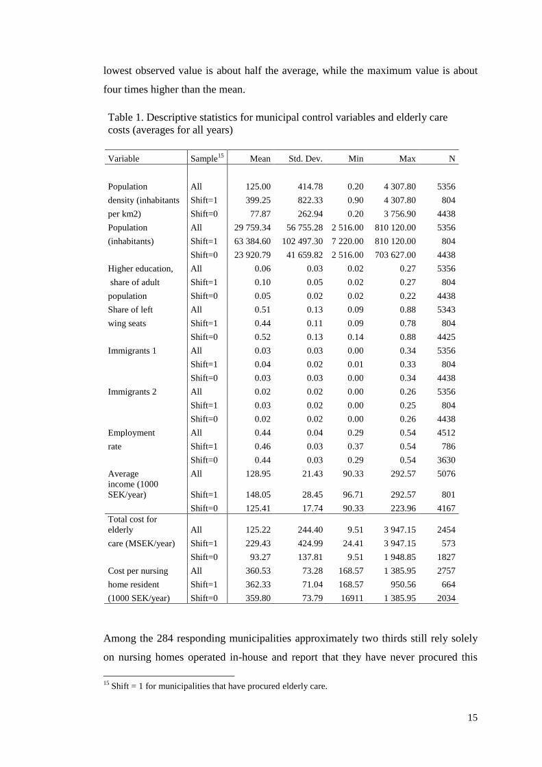
The distribution of cost per resident is wide. The average annual cost per person in a

nursing home is 359,150 SEK (at 1990 prices; close to € 60,000 at 2011 prices). The

15

lowest observed value is about half the average, while the maximum value is about

four times higher than the mean.

Table 1. Descriptive statistics for municipal control variables and elderly care

costs (averages for all years)

Variable Sample15

Mean Std. Dev. Min Max N

Population All 125.00 414.78 0.20 4 307.80 5356

density (inhabitants Shift=1 399.25 822.33 0.90 4 307.80 804

per km2) Shift=0 77.87 262.94 0.20 3 756.90 4438

Population All 29 759.34 56 755.28 2 516.00 810 120.00 5356

(inhabitants) Shift=1 63 384.60 102 497.30 7 220.00 810 120.00 804

Shift=0 23 920.79 41 659.82 2 516.00 703 627.00 4438

Higher education, All 0.06 0.03 0.02 0.27 5356

share of adult Shift=1 0.10 0.05 0.02 0.27 804

population Shift=0 0.05 0.02 0.02 0.22 4438

Share of left All 0.51 0.13 0.09 0.88 5343

wing seats Shift=1 0.44 0.11 0.09 0.78 804

Shift=0 0.52 0.13 0.14 0.88 4425

Immigrants 1 All 0.03 0.03 0.00 0.34 5356

Shift=1 0.04 0.02 0.01 0.33 804

Shift=0 0.03 0.03 0.00 0.34 4438

Immigrants 2 All 0.02 0.02 0.00 0.26 5356

Shift=1 0.03 0.02 0.00 0.25 804

Shift=0 0.02 0.02 0.00 0.26 4438

Employment All 0.44 0.04 0.29 0.54 4512

rate Shift=1 0.46 0.03 0.37 0.54 786

Shift=0 0.44 0.03 0.29 0.54 3630

Average All 128.95 21.43 90.33 292.57 5076

income (1000

SEK/year) Shift=1 148.05 28.45 96.71 292.57 801

Shift=0 125.41 17.74 90.33 223.96 4167

Total cost for

elderly All 125.22 244.40 9.51 3 947.15 2454

care (MSEK/year) Shift=1 229.43 424.99 24.41 3 947.15 573

Shift=0 93.27 137.81 9.51 1 948.85 1827

Cost per nursing All 360.53 73.28 168.57 1 385.95 2757

home resident Shift=1 362.33 71.04 168.57 950.56 664

(1000 SEK/year) Shift=0 359.80 73.79 16911 1 385.95 2034

Among the 284 responding municipalities approximately two thirds still rely solely

on nursing homes operated in-house and report that they have never procured this

15 Shift = 1 for municipalities that have procured elderly care.

16

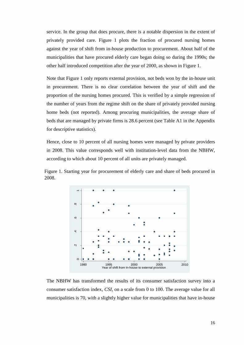
service. In the group that does procure, there is a notable dispersion in the extent of

privately provided care. Figure 1 plots the fraction of procured nursing homes

against the year of shift from in-house production to procurement. About half of the

municipalities that have procured elderly care began doing so during the 1990s; the

other half introduced competition after the year of 2000, as shown in Figure 1.

Note that Figure 1 only reports external provision, not beds won by the in-house unit

in procurement. There is no clear correlation between the year of shift and the

proportion of the nursing homes procured. This is verified by a simple regression of

the number of years from the regime shift on the share of privately provided nursing

home beds (not reported). Among procuring municipalities, the average share of

beds that are managed by private firms is 28.6 percent (see Table A1 in the Appendix

for descriptive statistics).

Hence, close to 10 percent of all nursing homes were managed by private providers

in 2008. This value corresponds well with institution-level data from the NBHW,

according to which about 10 percent of all units are privately managed.

Figure 1. Starting year for procurement of elderly care and share of beds procured in

2008.

The NBHW has transformed the results of its consumer satisfaction survey into a

consumer satisfaction index, CSI, on a scale from 0 to 100. The average value for all

municipalities is 70, with a slightly higher value for municipalities that have in-house

0.2

.4.6

.81

Share

of beds o

pera

ted b

y p

rivate

fir

ms in 2

008

1990 1995 2000 2005 2010Year of shift from in-house to external provision

17

production only than for procuring municipalities. The difference is, however, not

statistically significant (the t-value is 1.2).16

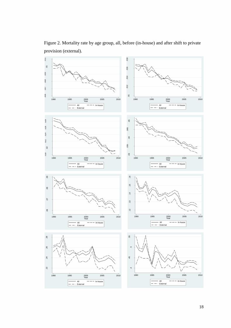
Figure 2 shows the development of annual mortality rate for the eight five-year age

groups we are primarily interested in. Generally, mortality rates have fallen between

1990 and 2009. Also, for all age groups, mortality rates tend to be markedly higher in

municipalities that have in-house production than in procuring municipalities

(external). However, the graphs do not reveal whether this is because procurement

results in lower mortality (a causal effect) or whether municipalities with low

mortality tend to procure (a selection effect). A municipality that begins procurement

during the 1990 to 2009 period will contribute to the “in-house” average for the first

few years, before the first procurement, and to the “external” average for the

subsequent years. Hence, the curve representing mortality in municipalities with

external provision is based on very few observations initially, rising to about a third

of the whole sample in 2009.

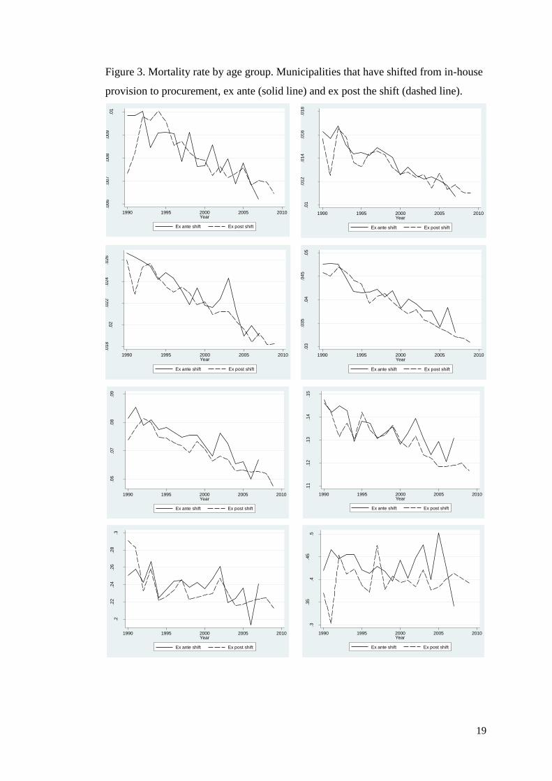
Figure 3 displays the mortality rate for only those municipalities that shift from in-

house to private regime. The solid line represents the municipalities before they shift

to procurement and the dashed line represents them after they have shifted. One (1)

municipality had shifted to procurement already in 1990. By 2008 all municipalities

in our sample that eventually introduced procurement had done so; hence the line

representing as yet pre-reform municipalities disappears after 2007. Visual

inspection of the graphs suggests that procurement is associated with lower mortality

rates.

16

We treat each municipality as an observation, independently drawn from an infinitely large

population.

18

Figure 2. Mortality rate by age group, all, before (in-house) and after shift to private

provision (external).

.006

.007

.008

.009

.01

.011

Mort

alit

y r

ate

age 6

0 to 6

4

1990 1995 2000 2005 2010Year

All In-house

External

.01

.012

.014

.016

.018

Mort

alit

y r

ate

age 6

5 to 6

91990 1995 2000 2005 2010

Year

All In-house

External

.018

.02

.022

.024

.026

.028

Mort

alit

y r

ate

age 7

0 to 7

4

1990 1995 2000 2005 2010Year

All In-house

External

.03

.035

.04

.045

.05

Mort

alit

y r

ate

age 7

5 to 7

9

1990 1995 2000 2005 2010Year

All In-house

External

.06

.07

.08

.09

Mort

alit

y r

ate

age 8

0 to 8

4

1990 1995 2000 2005 2010Year

All In-house

External

.12

.13

.14

.15

.16

Mort

alit

y r

ate

age 8

5 to 8

9

1990 1995 2000 2005 2010Year

All In-house

External

.22

.24

.26

.28

Mort

alit

y r

ate

age 9

0 to 9

4

1990 1995 2000 2005 2010Year

All In-house

External

.4.4

5.5

.55

Mort

alit

y r

ate

age 9

5 p

lus

1990 1995 2000 2005 2010Year

All In-house

External

19

Figure 3. Mortality rate by age group. Municipalities that have shifted from in-house

provision to procurement, ex ante (solid line) and ex post the shift (dashed line).

.006

.007

.008

.009

.01

Mort

alit

y r

ate

age 6

0 to 6

4

1990 1995 2000 2005 2010Year

Ex ante shift Ex post shift

.01

.012

.014

.016

.018

Mort

alit

y r

ate

age 6

5 to 6

9

1990 1995 2000 2005 2010Year

Ex ante shift Ex post shift

.018

.02

.022

.024

.026

Mort

alit

y r

ate

age 7

0 to 7

4

1990 1995 2000 2005 2010Year

Ex ante shift Ex post shift

.03

.035

.04

.045

.05

Mort

alit

y r

ate

age 7

4 to 7

9

1990 1995 2000 2005 2010Year

Ex ante shift Ex post shift

.06

.07

.08

.09

Mort

alit

y r

ate

age 8

0 to 8

4

1990 1995 2000 2005 2010Year

Ex ante shift Ex post shift

.11

.12

.13

.14

.15

Mort

alit

y r

ate

age 8

5 to 8

9 p

lus

1990 1995 2000 2005 2010Year

Ex ante shift Ex post shift

.2.2

2.2

4.2

6.2

8.3

Mort

alit

y r

ate

age 9

0 to 9

4

1990 1995 2000 2005 2010Year

Ex ante shift Ex post shift

.3.3

5.4

.45

.5

Mort

alit

y r

ate

age 9

5 p

lus

1990 1995 2000 2005 2010Year

Ex ante shift Ex post shift

20

5. Empirical approach

We identify the effect of procurement from the municipality-wide changes in

mortality following procurement, relative to contemporaneous changes in mortality

among municipalities that have not shifted from in-house to external provision, i.e.,

with a difference-in-difference approach.17

As already mentioned, using

municipality-wide mortality rates largely avoids the problems of selection effects,

since less than two out of one thousand elderly in permanent homes receive elderly

care outside of their home municipalities.

We argue that mortality can be seen as a relatively objective measure of non-

contractible quality. It is widely used as a quality indicator for medical and related

services and it has the interesting property that it is observable to us, in the sense that

it is amenable to statistical analysis, while it most likely cannot be contracted upon,

for two reasons. First, because the relationship between mortality and elderly care

quality is noisy, the number of patients would be too small within an individual

provider-municipality relation to allow for significant inference and, hence, for

effective incentive mechanisms to be linked to mortality. Second, explicit rewards

(sanctions) linked to survival (mortality) would give providers incentives to screen

patients. And even if mortality was in principle contractible, we know from the direct

inspection of contracts that it was not contracted for in our data, so that it would still

be a relatively good proxy for effects on other non-contractible quality dimensions.

Mortality panel data analysis

We opt for a random-effect model, rather than a fixed-effect model, trading a risk for biased

estimates for the higher efficiency of the former model. To eliminate bias as far as possible,

we include socio-economic variables such as educational level. Furthermore, while the

fixed-effect model eliminates bias from time-constant non-observables that are correlated

with the decision to procure, it will not eliminate bias from non-observables that are not

constant over time and that are correlated with the key explanatory variable (here, the shift to

procurement). Hence, as will be discussed further in Section 7, we strive to control for

factors that are not constant over time and that are likely to be correlated with the decision to

procure.18

17 Sommers et al, 2012, uses similar methods to assess the impact of expanded Medicaid eligibility. 18 Our modeling choice is supported by the Hausman test in …[x out of y age groups?]

21

The effect of a shift to procurement on mortality is estimated with feasible

generalized least square (FGLS). We weigh municipalities with the square root of the

population, since mortality rates will be more precise in larger municipalities, and we

depart from a heteroskedastic model, since the variance differs between

municipalities. All continuous variables are measured in logarithms.

Behind the choice of five-year age groups is a balance between having a sufficient

number of observations in each group and taking into account differences in health

needs between elderly of different ages. For small municipalities, the proportion of

zeros is high for the oldest age groups. This is unfortunate because the model is

logarithmic. Hence, we base our estimates on survival rate (SURV), which for age

group i in municipality m at time t is defined as:

(1)

where Population is measured at the start of year t. Expression (2) specifies the

model used for estimating survival over the 1993-2009 period.19

∑

(2)

where i=1,…,9 represents age group, each group compromises five years;

m=1,…,276 represents municipality; t=1,…,17 corresponds to the 1993-2009 time

period and TD represents time dummy variables. The dummy variable Smt assumes a

value of 1 if elderly care in municipality m has been procured at time t. Municipality-

and-time-specific control variables are the population density (Dmt), the share of the

population with more than three years of university studies (higher education, HEmt),

the employment rate (Emt) and the share of immigrants aged 65 and above (IMmt).20

19 The descriptive statistics and the graphs represent the period 1990 to 2009 but the long panel in the

estimations represent the 1993 to 2009 period. This is due to lack of data on the employment rate for

the first three years. 20

The immigrant variable is the share immigrants aged 65 and above when the estimations are

performed for the 7 oldest age groups and the immigrants aged 55 to 64 when the estimations are

performed for the two youngest age groups.

22

The political situation in the local council is also controlled for. It is defined as the

left wing, or socialist parties’ share of the seats in the local council, LWmt.

The error structure is given by

(3)

where αm is a municipal-specific random effect and εmt is white noise – a municipal-

and-time-specific error term.

The regression model is estimated for each of the nine age groups (55 to 59, 60 to 64,

65 to 69, 70 to 74, 75 to 79, 80 to 84, 85 to 89, 90 to 94, and 95 plus).21

The effect of

procurement on the specific age group is estimated by 1.22

A positive and significant

effect of shift (S) would indicate higher quality (higher survival rate, or lower

mortality) in a specific age group and vice versa.

Based on the graphs in Figure 3 and Figure 4 our prior is that 1 will be significant

and positive at least for the age groups where we find a sizeable share of the

population in nursing homes, i.e., age groups 85 to 89 and above. We expect no

significant effect of shift in age groups 55 to 59 years old and 60 to 64 years old. We

expect no or very small effects in age group 65 to 69 due to the low share of the

population in nursing home care, less than one percent (see Table A1 in the

Appendix). The diff-in-diff methodology allows us to control for time-constant

unobserved variation across municipalities.

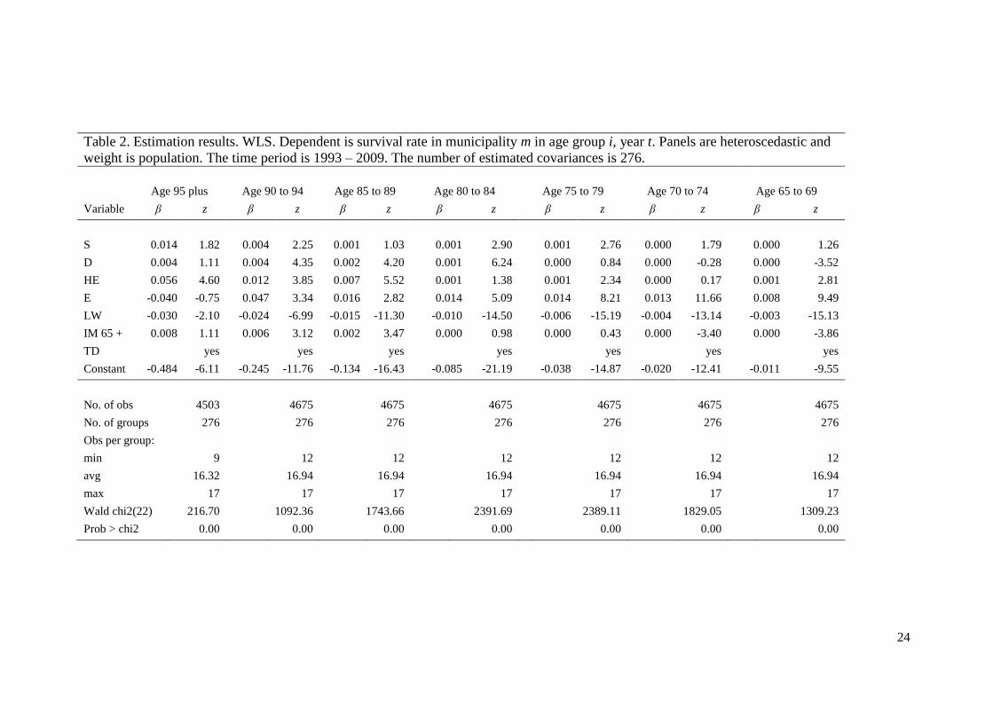
6. Results: Survival and external provision

Expression (2) is estimated separately for each of the nine age groups and results are

presented in Table 2. No significant effect of shift is found for the youngest age

groups 55 to 59, 60 to 64 and 65 to 69, respectively. The results for the two youngest

age groups are not reported in the table.

However, there is a significant effect on the survival in all of the more senior age

groups, except the age group 85 to 89 years, although the significance level is lower

for age groups 95-plus (6.8 percent) and 70 to 74 (7.3 percent). The coefficients

21 We suppress the age-group index. 22

In the standard notation of the diff-in-diff literature, S is the interaction of a treatment-group dummy

and a post-treatment time dummy.

23

suggest a 1.4 to less than 0.1 percent effect on survival due to a shift from in-house

regime to procurement, with larger effects for the more senior age groups, consistent

with the fact that the fraction that receives care in nursing homes rises with age.

24

Table 2. Estimation results. WLS. Dependent is survival rate in municipality m in age group i, year t. Panels are heteroscedastic and

weight is population. The time period is 1993 – 2009. The number of estimated covariances is 276.

Age 95 plus Age 90 to 94 Age 85 to 89 Age 80 to 84 Age 75 to 79 Age 70 to 74 Age 65 to 69

Variable β z β z β z β z β z β z β z

S 0.014 1.82 0.004 2.25 0.001 1.03 0.001 2.90 0.001 2.76 0.000 1.79 0.000 1.26

D 0.004 1.11 0.004 4.35 0.002 4.20 0.001 6.24 0.000 0.84 0.000 -0.28 0.000 -3.52

HE 0.056 4.60 0.012 3.85 0.007 5.52 0.001 1.38 0.001 2.34 0.000 0.17 0.001 2.81

E -0.040 -0.75 0.047 3.34 0.016 2.82 0.014 5.09 0.014 8.21 0.013 11.66 0.008 9.49

LW -0.030 -2.10 -0.024 -6.99 -0.015 -11.30 -0.010 -14.50 -0.006 -15.19 -0.004 -13.14 -0.003 -15.13

IM 65 + 0.008 1.11 0.006 3.12 0.002 3.47 0.000 0.98 0.000 0.43 0.000 -3.40 0.000 -3.86

TD yes yes yes yes yes yes yes

Constant -0.484 -6.11 -0.245 -11.76 -0.134 -16.43 -0.085 -21.19 -0.038 -14.87 -0.020 -12.41 -0.011 -9.55

No. of obs 4503 4675 4675 4675 4675 4675 4675

No. of groups 276 276 276 276 276 276 276

Obs per group:

min 9 12 12 12 12 12 12

avg 16.32 16.94 16.94 16.94 16.94 16.94 16.94

max 17 17 17 17 17 17 17

Wald chi2(22) 216.70 1092.36 1743.66 2391.69 2389.11 1829.05 1309.23

Prob > chi2 0.00 0.00 0.00 0.00 0.00 0.00 0.00

25

Although we are mainly interested in the effect of the shift variable and view the

other variables as controls, we comment briefly on them. Most of them are

significant and have the expected signs. More than three years of university level

education seems to affect the survival rate in a positive direction. The only

exceptions are age groups 80 to 84 and 70 to 74, respectively.

Higher employment rate is associated with higher survival rate for all age groups but

the oldest one (95 plus). High population density decreases survival rates for the

younger age groups, 65 years and less, while it has no or the opposite effect for the

five oldest age groups. A higher socialist representation in the local council is

associated with lower survival rate. The survival rate generally increases with the

fraction of immigrants in the older age groups and decreases for the younger ones.

The coefficients for the year dummies (not reported) indicate a clearly increasing

trend in the survival rate.

An indication of the magnitude of the effect among those directly concerned can be

obtained by dividing the estimated effect (as reported in the top row of Table 2) with

the fraction of the population living in nursing home (Table A2 in the Appendix).

According to this measure mortality is reduced by 1-3 percent, corresponding to a

life-expectancy increase of two-three weeks after admittance to a nursing home. If

we allocate the effect only to residents of procured elderly homes, assuming no

impact on the municipalities’ in-house units, the mortality reduction would be about

three times as large for those concerned and the life-time extension would be around

two months.

7. Extending the empirical analysis

There are at least three possible objections to our result. First, the effect could be due

to differences in mortality or survival trends between procuring and non-procuring

municipalities. Second, the decision to procure could be correlated with changes in

expenditure. Third, it may be that while survival increases, quality deteriorates in

other dimensions.

Addressing these concerns will also take us some way towards an understanding of

the mechanisms behind the improvements observed after procurement, given that the

results are robust to the three objections just mentioned. The most obvious

26

mechanism is that private firms are simply more efficient. Alternatively, the

procurement process may compel the procuring authority to be systematic about care

practices and quality standards and this effort may spill over also to the in-house

units. A third explanation is that poorly performing units – with weak managers or

dysfunctional “corporate” cultures – are the first to be targeted for procurement. If an

adverse selection is replaced with average-quality units this will show up as an

improvement.

Differential mortality trends

It has been suggested that the mortality may have been falling faster among well-

educated citizens than among others.23

Since municipalities that procure tend to have

better educated and richer voters the shift variable could then pick up this trend

divergence and erroneously lead us to conclude that procurement improves survival.

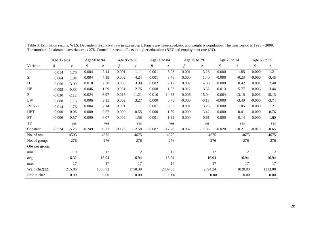
To address this possible problem, we introduce a variable, HET, that allows the

effect of higher education to vary over time. The variable is defined as the share of

higher education times a trend variable. In a similar manner the effect of education is

also allowed to vary over time by inclusion of a variable defined as the share of

population employed times a trend variable (ET). Equation (2) is repeated below as

equation (4) with the new variables included.

∑

(4)

where i=1,…,9 represents age group, each group compromises five years;

m=1,…,276 represents municipality; t=1,…,17 corresponds to the 200-2009 time

period.

As can be seen in Table 3 and in contracts to Shkolnikov et al. (2011), there is no

clear evidence of an increased positive effect of education, since the HET coefficient

is insignificant. This could be explained by the differences in the approach, the data

used and the periods of observation. (Their estimations build on the population in the

Nordic countries aged 40 and above and separate analyses are performed for men

and women.) There is one exception: the coefficient for age 75 to 79. The HET

23 Sholnikov et al, (2011).

27

coefficient is significant and negative for this age group, contrary to our

expectations. Further, there is no evidence of an increased positive effect of

employment, since the ET coefficient is insignificant.

28

Table 3. Estimation results. WLS. Dependent is survival rate in age group i. Panels are heteroscedastic and weight is population. The time period is 1993 – 2009.

The number of estimated covariances is 276. Control for trend effects in higher education (HET and employment rate (ET).

Age 95 plus Age 90 to 94 Age 85 to 89 Age 80 to 84 Age 75 to 79 Age 70 to 74 Age 65 to 69

Variable β z β z β z Β z β z β z β z

0.014 1.76 0.004 2.14 0.001 1.11 0.001 3.03 0.001 3.26 0.000 1.85 0.000 1.21

S 0.004 1.04 0.004 4.19 0.002 4.24 0.001 6.46 0.000 1.40 -0.000 -0.23 -0.000 -3.45

D 0.056 3.09 0.010 2.30 0.006 3.39 0.002 2.12 0.002 4.00 0.000 0.42 0.001 2.48

HE -0.095 -0.88 0.046 1.59 0.031 2.76 0.008 1.53 0.012 3.62 0.013 5.77 0.006 3.44

E -0.030 -2.12 -0.024 -6.97 -0.015 -11.21 -0.010 -14.63 -0.006 -15.04 -0.004 -13.15 -0.003 -15.13

LW 0.008 1.15 0.006 3.15 0.002 3.27 0.000 0.78 -0.000 -0.15 -0.000 -3.40 -0.000 -3.74

IM 65 + 0.014 1.76 0.004 2.14 0.001 1.11 0.001 3.03 0.001 3.26 0.000 1.85 0.000 1.21

HET 0.000 0.06 0.000 0.57 0.000 0.55 -0.000 -1.59 -0.000 -3.42 -0.000 -0.41 -0.000 -0.76

ET 0.006 0.57 0.000 0.07 -0.002 -1.56 0.001 1.22 0.000 0.61 0.000 0.14 0.000 1.60

TD yes yes yes yes yes yes yes

Constant -0.524 -5.23 -0.249 -9.77 -0.125 -12.58 -0.087 -17.78 -0.037 -11.85 -0.020 -10.21 -0.013 -8.65

No. of obs 4503 4675 4675 4675 4675 4675 4675

No. of groups 276 276 276 276 276 276 276

Obs per group:

min 9 12 12 12 12 12 12

avg 16.32 16.94 16.94 16.94 16.94 16.94 16.94

max 17 17 17 17 17 17 17

Wald chi2(22) 215.86 1080.72 1750.39 2409.63 2394.24 1828.00 1313.08

Prob > chi2 0.00 0.00 0.00 0.00 0.00 0.00 0.00

29

Contemporaneous expenditure shifts

Another possible weakness of our method is that there could be shocks that impact

both on our measure of quality (survival) and on the regime choice. For example, a

negative budget shock could trigger a transition to procurement and cuts in the

budget for elderly care. Alternatively, given the apparent positive effect of

procurement, the politicians may have “bribed” their constituencies into accepting

procurement by simultaneously increasing spending on elderly care. A statistical

analysis could then lead to the erroneous conclusion that procurement causes

changes in non-contractible quality. To resolve this concern as far as possible, we

control for expenditures per client in elderly care.

For the 2000-2009 time period we have, for each municipality, access to average

costs for nursing-home care and the number of residents in different age group. We

use this information to define two indices: a cost index (COSTI) and an admission-

policy index (RESI). The cost index measures the municipality’s actual cost per

resident relative to the average cost for a municipality with similar population

composition; the admission-policy index measures the municipality’s relative

generosity in admitting elderly to nursing homes. The exact definitions are provided

in the Appendix.

As a first step, we estimate the effect of the shift to procurement on costs. We

estimate the following regression equations, using either the municipality’s total cost

for nursing home care (COSTT), or the total cost per nursing home resident (COSTR)

in municipality m at time t, as the dependent variable:

(5)

(6)

where m=1,…,276 and t=2000,…,2009 and

(7)

As above αm is the random effect and εmt is white noise. The effect of procurement on

cost is estimated by 1. In addition to the controls used above, the total-cost model

30

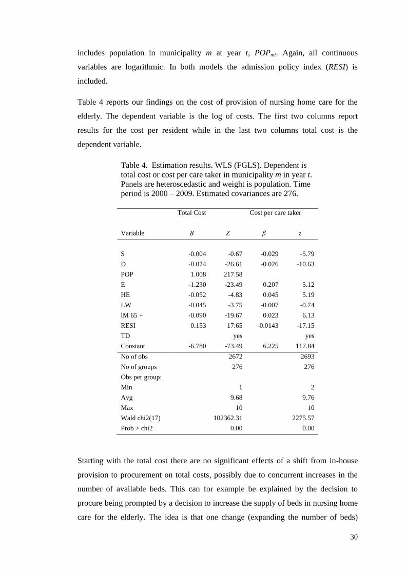
includes population in municipality m at year t, POPmt. Again, all continuous

variables are logarithmic. In both models the admission policy index (RESI) is

included.

Table 4 reports our findings on the cost of provision of nursing home care for the

elderly. The dependent variable is the log of costs. The first two columns report

results for the cost per resident while in the last two columns total cost is the

dependent variable.

Table 4. Estimation results. WLS (FGLS). Dependent is

total cost or cost per care taker in municipality m in year t.

Panels are heteroscedastic and weight is population. Time

period is 2000 – 2009. Estimated covariances are 276.

Total Cost Cost per care taker

Variable Β Z β z

S -0.004 -0.67 -0.029 -5.79

D -0.074 -26.61 -0.026 -10.63

POP 1.008 217.58

E -1.230 -23.49 0.207 5.12

HE -0.052 -4.83 0.045 5.19

LW -0.045 -3.75 -0.007 -0.74

lM 65 + -0.090 -19.67 0.023 6.13

RESI 0.153 17.65 -0.0143 -17.15

TD yes yes

Constant -6.780 -73.49 6.225 117.84

No of obs 2672 2693

No of groups 276 276

Obs per group:

Min 1 2

Avg 9.68 9.76

Max 10 10

Wald chi2(17) 102362.31 2275.57

Prob > chi2 0.00 0.00

Starting with the total cost there are no significant effects of a shift from in-house

provision to procurement on total costs, possibly due to concurrent increases in the

number of available beds. This can for example be explained by the decision to

procure being prompted by a decision to increase the supply of beds in nursing home

care for the elderly. The idea is that one change (expanding the number of beds)

31

prompts another change (change of type of provision). Another plausible explanation

is that private providers have stronger incentives to maintain full occupancy. There is

no apparent contradiction between these two possible explanations.

The cost-per-resident shift coefficient clearly suggests that private provision leads to

a reduction in cost per resident. The estimated cost reduction is 3.0 percent. Taken

together with the results showing a fall in mortality, procurement of elderly care

seems to reduce cost per resident at the same time as it increases quality.

Commenting briefly on our control variables, we find that high population density

and large representation of socialist parties is associated with lower costs per resident

and lower total costs. Educational level, share of immigrants and employment rate

are associated with higher costs per resident, but have no significant effect on total

costs. A more generous admittance policy is associated with lower costs per resident

and higher total costs, suggesting that elderly with better health status are admitted.

Additionally, to check the robustness of the finding that a shift from in-house to

private provision seems to decrease mortality we include the cost index (COSTI) and

the admission index (RESI) in a modified survival equation (see expression (2) for

the original model):

∑

(8)

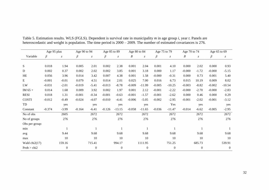
where i=1,…,9; m=1,…,276; t=2000,…,2009 and with variables as defined above.

The extended model can only be estimated over the 2000 to 2009 period. The results

are reported in Table 5.

The coefficients for shift for the different age groups confirm the previous findings:

there is a positive and significant effect on the survival rate in all age groups aged 70

and above. The coefficients for the four oldest age groups are significant at the 5.3,

4.5, 1.7 and 4.1percent level, respectively. The magnitude is similar to that found for

the long panel.

32

Table 5. Estimation results. WLS (FGLS). Dependent is survival rate in municipality m in age group i, year t. Panels are

heteroscedastic and weight is population. The time period is 2000 – 2009. The number of estimated covariances is 276.

Age 95 plus Age 90 to 94 Age 85 to 89 Age 80 to 84 Age 75 to 79 Age 70 to 74 Age 65 to 69

Variable β z β z β z Β z β z Β z β z

S 0.018 1.94 0.005 2.01 0.002 2.38 0.001 2.04 0.001 4.10 0.000 2.02 0.000 0.93

D 0.002 0.37 0.002 2.02 0.002 3.85 0.001 3.18 0.000 1.17 -0.000 -1.72 -0.000 -5.15

HE 0.056 3.96 0.014 3.42 0.007 4.38 0.001 1.58 -0.000 -0.31 0.000 0.73 0.001 5.40

E -0.001 -0.01 0.079 4.51 0.014 2.01 0.025 7.00 0.016 6.73 0.015 10.19 0.009 8.02

LW -0.031 -2.01 -0.019 -5.41 -0.013 -8.78 -0.009 -11.99 -0.005 -10.25 -0.003 -8.82 -0.002 -10.54

IM 65 + 0.014 1.68 0.009 3.92 0.002 1.97 0.001 2.12 -0.001 -2.22 -0.000 -2.70 -0.000 -2.83

RESI 0.018 1.31 -0.001 -0.34 -0.001 -0.63 -0.001 -1.57 -0.001 -2.62 0.000 0.46 0.000 0.29

COSTI -0.012 -0.49 -0.024 -4.07 -0.010 -4.41 -0.006 -5.05 -0.002 -2.95 -0.001 -2.02 -0.001 -3.12

TD yes yes yes yes Yes yes yes

Constant -0.374 -3.99 -0.164 -6.41 -0.126 -13.15 -0.058 -11.65 -0.036 -11.47 -0.014 -6.62 -0.005 -2.95

No of obs 2605 2672 2672 2672 2672 2672 2672

No of groups 276 276 276 276 276 276 276

Obs per group:

min 1 1 1 1 1 1 1

avg 9.44 9.68 9.68 9.68 9.68 9.68 9.68

max 10 10 10 10 10 10 10

Wald chi2(17) 159.16 715.41 994.17 1111.95 751.25 685.73 539.91

Prob > chi2 0 0 0 0 0 0 0

33

Somewhat surprisingly, the cost index coefficient indicates a negative relationship

between expenditures and survival rate. It is negative and significant for all age

groups but the 95-plus-years-olds. Our interpretation is that poor health drives

expenditures and mortality. The coefficient of RESI is significant only for the age

group 75 to 79, for which the coefficient is negative.

The results for the socioeconomic factors and year dummy variables are qualitatively

the same as for the longer panel and are therefore not commented upon.

Other quality dimensions – perceived quality

The municipality’s CSI, Consumer Satisfaction Index, is a subjective measure of

perceived quality. One may argue that perhaps higher mortality is linked to better

service provision in other dimensions, for example more freedom to go out walking

under the risk of catching a cold and then pneumonia. The CSI, however, will allow

us to control also for this.

Customer satisfaction – cross-section analysis

We do not have access to panel data for the CSI. Hence, we estimate the following

equation on 2008 cross-sectional data:

∑

∑

(9)

Except for some additions, variables and notation are as above, with t suppressed.

Socio-economic factors have been shown to affect patient satisfaction in elderly

people and therefore controlled for. (E.g., Lee and Kasper, 1998.) We add seven

quality indicators for elderly care (QYm) provided by the NBHW. The definitions of

the quality variables are found in Table A1 in the Appendix. In addition, five health

related factors, such as use of pharmaceuticals, are also controlled for (MEDm). See

Table A1 in the Appendix for definition and descriptive statistics.

34

The quality and health related variables represent (objective and contractible) quality

indicators measured by the NBHW and SALAR,24

respectively, that mainly relate to

inputs. Equation (9) is first estimated using the socioeconomic factors only and then

estimated with QYm and MEDm included. This allows us to check for robustness in

the outcome with respect to systematic differences in quality and health indicators

with respect to type of provision.

None of the quality or health related parameters are too highly correlated to be

included in the regression equation (see Table A4 in the Appendix). Equation (9) is

also estimated including the share of beds procured (SP) and the experience of

procurement (EXP). The latter variable is defined as EXP = 2008 – year of shift.

Consumer satisfaction index as explained by type of provision

Consumer satisfaction is, in principle, a ranking variable, suggesting that a method

such as ordered probit or logit should be used. On the other hand, the large number

of possible outcomes and the fact that individual values are aggregated to the

municipal level suggest that OLS should be used. Table 6 reports ordinary least

square estimates. As reported above, the average CSI was observed to be slightly

lower among the procuring municipalities but the difference was not statistically

significant. After adding more controls (results are reported in Table A5 in the

Appendix), there is still no significant effect of the type of provision on the consumer

satisfaction index. This is also the case when the quality and health indicators are

excluded.

Of the socio-economic factors, only population density and the political situation in

the municipal council have significant effects on customer satisfaction. Higher

population density and larger share of the seats in the local council assigned to the

left wing are associated with less satisfaction.

Adding controls (see Table A5 in the Appendix for results) the coefficient for cost

index becomes significant at the five percent level, suggesting that generous

spending on nursing homes improves the CSI. The marginal effect on CSI of

doubling the spending, starting from the average expenditure level, is about three.

24

The Swedish Association of Local Authorities and Regions.

35

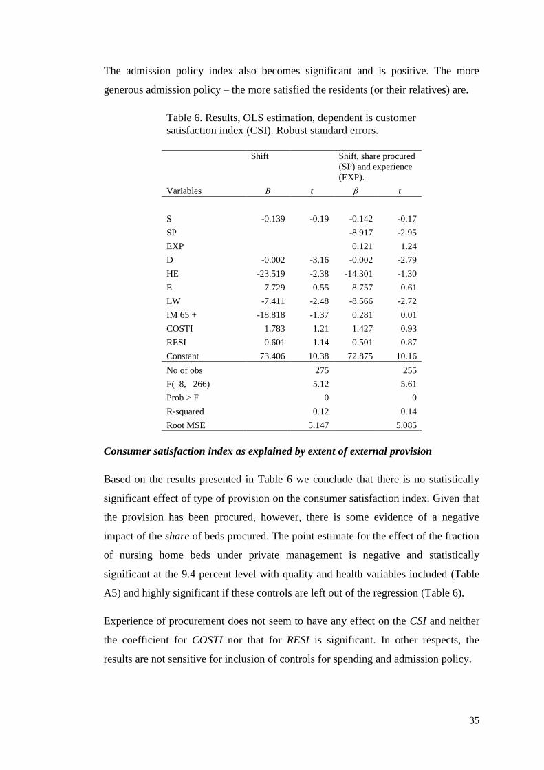
The admission policy index also becomes significant and is positive. The more

generous admission policy – the more satisfied the residents (or their relatives) are.

Table 6. Results, OLS estimation, dependent is customer

satisfaction index (CSI). Robust standard errors.

Shift Shift, share procured

(SP) and experience

(EXP).

Variables Β t β t

S -0.139 -0.19 -0.142 -0.17

SP

-8.917 -2.95

EXP

0.121 1.24

D -0.002 -3.16 -0.002 -2.79

HE -23.519 -2.38 -14.301 -1.30

E 7.729 0.55 8.757 0.61

LW -7.411 -2.48 -8.566 -2.72

IM 65 + -18.818 -1.37 0.281 0.01

COSTI 1.783 1.21 1.427 0.93

RESI 0.601 1.14 0.501 0.87

Constant 73.406 10.38 72.875 10.16

No of obs 275

255

F( 8, 266) 5.12

5.61

Prob > F

0

0

R-squared 0.12

0.14

Root MSE

5.147

5.085

Consumer satisfaction index as explained by extent of external provision

Based on the results presented in Table 6 we conclude that there is no statistically

significant effect of type of provision on the consumer satisfaction index. Given that

the provision has been procured, however, there is some evidence of a negative

impact of the share of beds procured. The point estimate for the effect of the fraction

of nursing home beds under private management is negative and statistically

significant at the 9.4 percent level with quality and health variables included (Table

A5) and highly significant if these controls are left out of the regression (Table 6).

Experience of procurement does not seem to have any effect on the CSI and neither

the coefficient for COSTI nor that for RESI is significant. In other respects, the

results are not sensitive for inclusion of controls for spending and admission policy.

36

Equation (9) is also estimated separately for only those municipalities that do procure

(dropping S from the regression equation) and controlling for degree of procurement

(SP) and experience. The results show (not reported) a negative effect of degree of

procurement and CSI and a model that seems to fit the data better. The explanatory

power increases from 14 percent to 41 percent.

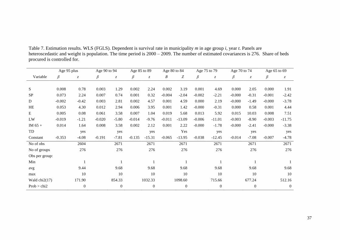
Towards an understanding of the mechanism – the effect of the share procured

In order to shed further light on the effect on mortality of procurement (Cf. Table 2),

equation (2) is also estimated with share of beds procured (SP). Again, due to data

availability this is performed for the shorter panel, 2000 to 2009. The results are

reported in Table 7.

The effect of shift is, with one exception, stable for the inclusion of share of beds

procured. The previously (Table 2) result of a 6.8 level significant effect for the 95

plus aged group is now lost. However, there is a significant and positive effect of

share of beds operated by private providers. For the other age groups the effect of

shift is stable and a negative (aged 80 to 84) or no effects of share of beds procured is

found.

The findings for the controls groups show a 5.7 percent significant and positive

effect of shift for the part of the population aged 65 to 69 (a group where we can find

a small fraction of nursing home residents) or no effect for the age groups outside the

nursing home care (results not reported). The other controls are not commented upon

as the outcome do not divert from the previous findings.

37

Table 7. Estimation results. WLS (FGLS). Dependent is survival rate in municipality m in age group i, year t. Panels are

heteroscedastic and weight is population. The time period is 2000 – 2009. The number of estimated covariances is 276. Share of beds

procured is controlled for.

Age 95 plus Age 90 to 94 Age 85 to 89 Age 80 to 84 Age 75 to 79 Age 70 to 74 Age 65 to 69

Variable β z β z β z Β Z β z β z β z

S 0.008 0.78 0.003 1.29 0.002 2.24 0.002 3.19 0.001 4.69 0.000 2.05 0.000 1.91

SP 0.073 2.24 0.007 0.74 0.001 0.32 -0.004 -2.04 -0.002 -2.21 -0.000 -0.31 -0.001 -2.42

D -0.002 -0.42 0.003 2.81 0.002 4.57 0.001 4.59 0.000 2.19 -0.000 -1.49 -0.000 -3.78

HE 0.053 4.30 0.012 2.94 0.006 3.95 0.001 1.42 -0.000 -0.31 0.000 0.58 0.001 4.44

E 0.005 0.08 0.061 3.58 0.007 1.04 0.019 5.68 0.013 5.92 0.015 10.03 0.008 7.51

LW -0.019 -1.21 -0.020 -5.80 -0.014 -9.76 -0.011 -13.09 -0.006 -11.01 -0.003 -8.90 -0.003 -11.75

IM 65 + 0.014 1.64 0.008 3.58 0.002 2.12 0.001 2.22 -0.000 -1.78 -0.000 -2.41 -0.000 -3.38

TD yes yes yes Yes yes yes yes

Constant -0.353 -4.08 -0.191 -7.81 -0.135 -15.31 -0.065 -13.95 -0.038 -12.45 -0.014 -7.08 -0.007 -4.78

No of obs 2604 2671 2671 2671 2671 2671 2671

No of groups 276 276 276 276 276 276 276

Obs per group:

Min 1 1 1 1 1 1 1

avg 9.44 9.68 9.68 9.68 9.68 9.68 9.68

max 10 10 10 10 10 10 10

Wald chi2(17) 171.90 854.33 1032.33 1098.60 715.66 677.24 512.16

Prob > chi2 0 0 0 0 0 0 0

38

8. Discussion and conclusions

Somewhat contrary to our expectations and to some of the theoretical predictions, we

find evidence suggesting that non-contractible quality increases following

procurement. Survival improvements are concentrated to the age groups where

nursing home residency is common. We arrive at our results after controlling for

municipality characteristics and year effects, using a difference-in-difference

random-effect approach. This finding is robust for controlling for trend specific

effect of socioeconomic factors (education and employment).

For a shorter panel we are able to control also for admittance policy and costs. We

find that per-resident costs fall after procurement, that total costs remain unchanged

and that higher costs are associated with a negative effect on survival. We interpret

the latter effect to be driven by variations in health status between municipalities:

poor health increases costs while reducing survival. Our main result, that

procurement increases survival, comes out even stronger in the shorter panel. This

finding is robust also for the inclusion of share of beds operated by private providers

– for all age groups but the oldest old. In that case, even though the there is an

insignificant effect of the shift to procurement, the results indicate that a higher share

of beds procured is associated with higher survival rate.

Using cross-sectional data, we find no statistically significant difference in customer

satisfaction between procuring and non-procuring municipalities. We do, however,

find that among procuring municipalities, those with a smaller share of procured

beds have more satisfied clients.

We conclude that procurement has increased quality (survival) while simultaneously

reducing costs per resident. There is, however, some indication that customer

satisfaction falls after procurement. A simple explanation is that efficiency increases

when production is transferred from in-house production units to private providers.

An alternative interpretation is that the decrease in mortality is due to the process that

precedes the procurement auction. The reform forces the municipalities to think

systematically about quality standards; standards that can be implemented also in

units that remain in-house. Yet other interpretations are that it is competition rather

39

than procurement that improves quality and that procurement is selectively used to

oust under-performing management.25

As mentioned, during most of the period we have studied the public procurement

rules were rather liberal, in the sense that the buyer had relatively large freedom to

select the winner. This may have allowed buyers to maintain quality through

informal reputational threats; and may have reduced competition and curbed cost

efficiencies. The fact that procured elderly care during our period of study was

expanding rapidly further boosted the importance of future sales relative to current

profitability. It will be interesting to see if our result holds up in a few years, when

EU’s new and stricter rules impose more rigid procedures aimed at open competition

and when the market has left the first expansionary phase. We conjecture that quality

degradation may become a problem in future, after the 2008 Procurement Act that

imposed stricter procedural rules limiting discretion and fostering open competition.

25 If competition were driving quality, however, we would expect to see higher survival rates in

densely populated municipalities – and we do not.

40

References

Amirkhanyan, Anna A., Hyun Joon Kim and Kristina T. Lambright, 2008, Does the

Public Sector Outperform the Nonprofit and For-Profit Sectors? Evidence from a

National Panel Study on Nursing Home Quality and Access, Journal of Policy

Analysis and Management, 27(2): 326-53.

Anderson, Randy I., H. Shelton Weeks and Bradley K. Hoobs, 2003, Nursing Home

Quality, Chain Affiliation, Profit Status and Performance, Journal of Real Estate

Research, 25(1): 43-60.

Angrist, Joshua, Eric Bettinger, Eric Bloom, Elizabeth King and Michael Kremer,

2002, Vouchers for Private Schooling in Colombia: Evidence from a Randomized

Natural Experiment, American Economic Review 92(5): 1535-1559.

Angrist, Joshua, Eric Bettinger and Michael Cremer, 2006, Long-Term Educational

Consequences of Secondary School Vouchers: Evidence from Administrative

Records in Colombia, American Economic Review 96(3): 847-862.

Bajari, Patrick and Steven Tadelis, 2001, Incentives versus Transaction Costs: A

Theory of Procurement Contracts, RAND Journal of Economics 32(3): 387-407.

Bajari, Patrick, Robert S. McMillan and Steven Tadelis, 2009, Auctions versus

Negotiations in Procurement: An Empirical Analysis, Journal of Law, Economics

and Organization, 25(2): 372-399.

Bajari, Patrick and Gregory Lewis, 2011, Procurement Contracting with Time

Incentives: Theory and Evidence, Quarterly Journal of Economics, 126 (3): 1173-1211.

Bandera, Oriana, Andrea Prat and Tommaso Valletti, 2009, Active and Passive

Waste in Government Spending: Evidence from a Policy Experiment, American

Economic Review, 99(4): 1278-1308.

Banfield, Edward C., 1975, Corruption as a Feature of Governmental Organization,

Journal of Law and Economics, 18(3): 587-605.

Bar-Isaac, Heski and Steven Tadelis, 2008, Seller Reputation, Foundations and

Trends in Microeconomics, 4(4): 273-351

41

Bayer, Patrick and David E. Pozen, 2005, The Effectiveness of Juvenile Correctional

Facilities: Public versus Private Management, Journal of Law & Economics, 48(2):

549-89.

Bédard, Kelly and H. E. Frech III, 2009, Prison Health Care: Is Contracting Out

Healthy? Health Economics, 18(11): 1248 – 1260.

Bergman, Mats A., 2008, Offentlig upphandling och offentliga inköp – omfattning

och sammansättning, Report to the Swedish Competition Authority (In Swedish)

Bergman, Mats A. and Sofia Lundberg, 2011, Tender Evaluation and Award

Methodolgies in Public Procurement, Umeå Economic Studies, No 821.

Boycko, Maxim, Andrei Shleifer and Robert W. Vishny, 1996, A Theory of

Privatisation, Economic Journal, 106(435): 309-19.

Calzolari, Giacomo, and Giancarlo Spagnolo, 2009, Relational Contracts and

Competitive Screening, CEPR Discussion Paper No. DP7434.

Chou, Shin-Yi, 2002, Asymmetric Information, Ownership and Quality of Care: An

Empirical Analysis of Nursing Homes, Journal of Health Economics, 21(2): 293-

311.

Cope, Stephen, 1995, Contracting-out in Local Government: Cutting by Privatizing,

Public Policy and Administration, 10(3): 29–44.

Grabowski, David C., 2004, A Longitudinal Study of Medicaid Payment, Private-

Pay Price and Nursing Home Quality, International Journal of Health Care Finance

and Economics, 4(1): 5-26.

Grabowski, David C. and David G. Stevenson, 2008, Ownership Conversion and

Nursing Home Performance, Health Services Research, 43(4): 1184-1203.

Gallo, William T., Elisabeth H. Bradley, Michele Siegel and Stanislav V. Kasi, 2000,

Health Effects of Involuntary Job Loss Among Older Workers: Findings From the

Health and Retirement Survey, Journal of Gerontology, 55B(3): 131-140.

42

Hart, Oliver, Andrei Shleifer and Robert W. Vishny, 1997, The Proper Scope of

Government: Theory and an Application to Prisons, Quarterly Journal of Economics,

112(4): 1127-1161.

Holmstrom, Bengt and Paul Milgrom, 1991, Multitask Principal–Agent Analyses:

Incentive Contracts, Asset Ownership, and Job Design, Journal of Law, Economics,

and Organization 7 (Special issue): 24-52.

Hsieh, Chang-Tai and Miguel Urquiola, 2006, The Effects of Generalized School

Choice on Achievement and Stratification: Evidence from Chile's Voucher Program,

Journal of Public Economics, 90(8-9): 1477-1503.

Iossa, Elisabetta and Patrick Rey, 2010, Building Reputation for Contract Renewal:

Implications for Performance Dynamics and Contract Duration, CEIS Research

paper No 155, University of Tor Vergata.

Jensen, Paul H. and Robin E. Stonecash, 2005, Incentives and the Efficiency of

Public Sector-outsourcing Contracts, Journal of Economic Surveys, 19(5): 767-787.

Kelman, Steven 1987, Public Choice and Public Spirit, The Public Interest, 87(2):

80-94.

Klein, Benjamin and Keith B. Leffler, 1981, The Role of Market Forces in Assuring

Contractual Performance, Journal of Political Economy, 89(4): 615-641.

Laffont, Jean-Jaques and Jean Tirole, 1993, A Theory of Incentives in Procurement

and Regulation, MIT Press, Cambridge, USA

Larsson, Kristina, Ingemar Kåreholt and Mats Thorslund, 2008, Care Utilisation in

the Last Years of Life in Relation to Age and Time to Death: Results from a Swedish

Urban Population of the Oldest Old, European Journal of Ageing, 5(4): 349–357.

Levin, Jonathan and Steven Tadelis, 2010, Contacting for Government Services:

Theory and Evidence from U.S Cities, Journal of Industrial Economics, 58(3): 507-

541.

43

Lee Yunhwan and Judith D. Kasper, 1998, Assessment of Medical Care by Elderly

People: General Satisfaction and Physician Quality, Health Services Research, 32(6):

741-758.

Lindqvist, Erik, 2008, Will Privatization Reduce Costs? IFN Working Paper No 736.

Macaulay, Stewart, 1963, Non-contractual Relations in Business: A Preliminary

Study, American Sociological Review, 28(1): 55 - 67.

MacLeod, W. Bentley, 2007, Reputations, Relationships, and Contract Enforcement,

Journal of Economic Literature, 45(3): 595-628.

Manelli, Alejandro M. and Daniel R. Vincent, 1995, Optimal Procurement

Mechanisms, Econometrica, 63(3): 591-620.

Ménard, Claude and Stephane Saussier, 2000, Contractual Choice and Performance:

The Case of Water Supply in France, Revue d'Economie Industrielle, 92: 385-404.

NBHW, 2008, Öppna jämförelser inom vården och omsorgen av äldre 2008.

Verksamhetens kvalitet. (In Swedish)

NBHW, 2009, Nationell brukarundersökning inom vården och omsorgen av äldre

2008. (In Swedish)

SALAR, 2007, Aktuellt på äldreområdet 2007. (In Swedish)

SALAR, 2008, Öppna Jämförelser 2008, Vård och omsorg om äldre. (In Swedish)

Shleifer, Andrei, 1998, State versus Private Ownership, Journal of Economic

Perspectives, 12(4): 133–150.

Shkolnikov, Vladimir, M. Evgueni, Andreev, Dimitrti A. Jdanov, Domantas

Jasilionis, Øystein Kravdal, Denny Vågerö and Tapini Valkonen, 2012, Increasing

Absolute Mortality Disparities by Education in Finland, Norway and Sweden, 1971-

2000, Journal of Epidemiology & Community Health, 66(4):372-8.

Sommers, Benjamin D., Katherine Baicker and Arnold M. Epstein, 2012, Mortality

and Access to Care among Adults after State Medicaid Expansions, The New

England Journal of Medicine, Special article, July 25.

44

Spulber, Daniel F., 1990, Auctions and Contract Enforcement, Journal of Law,

Economics, and Organization, 6(2): 325-344.

45

Appendix

Table A1. Descriptive statistics, cross sectional data on observable quality.

Min Max Mean Std.

dev.

N

CSI All Consumer satisfaction index based

on client survey.

56 88 70.90 5.42 283

Shift 56 87 70.33 5.02 94

No shift 57 88 71.15 5.60 189

Degree of

competition

Percentage of beds managed by

private firms.

SCORE FOR:

0 1 0.29 0.28 94

Participation Share of clients with an

implementation plan with active

participation of the client. 1.00 5.00 2.89 1.42 275

Staff density Staff per client. 1.00 5.00 3.01 1.40 275

Competence Share of regular staff with

vocational training at the secondary

level or similar; staff work

experience 1.00 5.00 2.94 0.95 276

Continuity Share of staff with full-tim

employment; staff turnover. 1.00 5.00 2.88 0.80 270

Privacy Private room and access to

individual hygiene and cooking

facilities. 1.00 4.80 3.07 0.78 264

Food Choice of meals; duration of night-

fasting period 2.30 5.00 3.47 0.80 262

Management Staff per manager. 1.00 5.00 2.86 1.39 274

Total risk PERCENTAGE OF RESIDENTS

With hazardous drug combinations. 0.01 0.06 0.03 0.01 274

Total ten Taking more than ten prescribed

drugs (80 years and older only) 0.06 0.21 0.12 0.03 274

Total three Taking three or more psychotropic

drugs (80 years and older only) 0.02 0.08 0.05 0.01 274

Stroke Assessing their health as very or

fairly good three months after

stroke (stroke patients only) 0.54 0.94 0.76 0.06 274

Hospital

PER 1000 POPULATION AGED

80 AND OLDER

Number of unplanned hospital

admissions 274.00 769.00 512.55 82.69 274

See NBHW (2008) and SALAR (2008) for full description of the surveys from which the data is

collected. The seven score variables are composite measures constructed by the NBHW; component

measures in italics are inversely related to the scores.

46

Treatment of costs and availability of beds

The variable COSTImt measures costs per bed and year and RESImt is a measure of

the number of residents at elderly-care homes per 100 inhabitants aged 65 or more.

Higher spending per resident is likely to increase quality (as shown by Grabowski,

2004, in his study of US nursery homes). However, costs per bed may be high also

because the municipality has a restrictive policy and only accepts clients in poor

health into nursing homes. Similarly, the number of residents per capita may be high

because the municipality has a population that is older than in most other

municipalities or because it has a generous admittance policy. For this reason,

COSTImt and RESImt are index variables, designed to measure the municipality’s

relative generosity in terms of spending per resident and in terms of accepting

residents, relative to an average municipality with the same population profile.

First, we model the expected number of residents per (1000) capita as follows:

(A1)

where ACTRES*mt is the expected number of residents per 1000 inhabitants in

municipality m at time t, calculated as the sum of the product of Pimt, population in

age group i, and the fraction of people in age group i living in elderly care at the

national level, . The values for the year 2007 are as shown in Table A2; we used

contemporaneous values in the estimations and interpolated for two years where data

was missing. Comparing actual number of residents, ACTRESmt, to the predicted

number gives us an index of the relative number of residents as

(A2)

If RESImt >1 the municipality m has an admittance policy that is more generous than

the average municipality and vice versa.

47

Table A2. The percentage of the population by age intervals living in nursery homes,

2007) (NBHW)

Age (years) Women Men All

65-74 0.912559 0.971143 0.941043

75-79 3.793745 3.149455 3.50845

80-84 9.186855 6.703249 8.183698

85-89 19.22256 12.48988 16.82569

90-94 34.3794 24.10474 31.41487

95- 50.22578 39.5069 47.9476

The cost per resident will increase if the average health status is reduced. We do not

know the health status of individuals, but we assume health deteriorates with age

and, therefore, that we can use the average age of the clients as a proxy for their

health. However, since we do not know average age either, we have to make

assumptions about that as well. We assume that average age can be approximated

as26

(A3)

using the notation from equation (A1) with Ai representing the average age in age

group i.27

That is, we assume that all municipalities admit fraction of its

population in age group i. We also assume that a more generous admittance policy,

i.e., a high value of RESI, implies that the average health status of the clients is

better. Hence, we model the cost per resident as

(A4)

where cmt is the per-client cost in municipality m at time t. Using the parameter

estimates of the model, we can predict the expected cost per resident in the

municipality as

(A5)

26

The average age of Swedes aged 95 or more is 97 years, as calculated from Statistics Sweden’s

population statistics. 27 We use the mid-point of the closed intervals and assume that the average age in the highest age

group is 97 years.

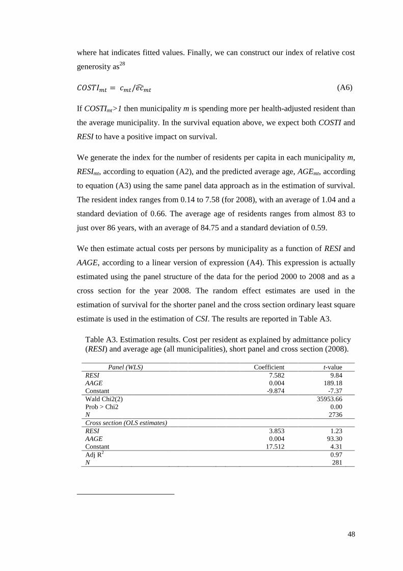
48

where hat indicates fitted values. Finally, we can construct our index of relative cost

generosity as28

(A6)

If COSTImt>1 then municipality m is spending more per health-adjusted resident than

the average municipality. In the survival equation above, we expect both COSTI and

RESI to have a positive impact on survival.

We generate the index for the number of residents per capita in each municipality m,

RESImt, according to equation (A2), and the predicted average age, AGEmt, according

to equation (A3) using the same panel data approach as in the estimation of survival.

The resident index ranges from 0.14 to 7.58 (for 2008), with an average of 1.04 and a

standard deviation of 0.66. The average age of residents ranges from almost 83 to

just over 86 years, with an average of 84.75 and a standard deviation of 0.59.

We then estimate actual costs per persons by municipality as a function of RESI and

AAGE, according to a linear version of expression (A4). This expression is actually

estimated using the panel structure of the data for the period 2000 to 2008 and as a

cross section for the year 2008. The random effect estimates are used in the

estimation of survival for the shorter panel and the cross section ordinary least square

estimate is used in the estimation of CSI. The results are reported in Table A3.

Table A3. Estimation results. Cost per resident as explained by admittance policy

(RESI) and average age (all municipalities), short panel and cross section (2008).

Panel (WLS) Coefficient t-value

RESI 7.582 9.84

AAGE 0.004 189.18

Constant -9.874 -7.37

Wald Chi2(2) 35953.66

Prob > Chi2 0.00

N 2736

Cross section (OLS estimates)

RESI 3.853 1.23

AAGE 0.004 93.30

Constant 17.512 4.31

Adj R2 0.97

N 281

49

None of the explanatory variables in cross section regression have a significant effect

on the cost per resident and the explanatory power of the model is poor. This is not

too problematic since the main point is to construct an index that can be used in the

regression of customer satisfaction index and mortality.

The cost per resident index has, as expected, a mean of one and it is distributed

between 0.49 and 2.31. The municipality with highest cost per resident spends

almost five times more than the municipality with the lowest cost per resident.

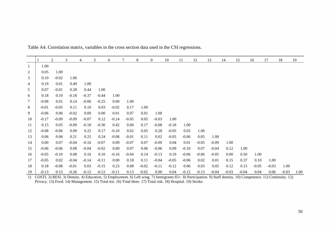
50

Table A4. Correlation matrix, variables in the cross section data used in the CSI regressions.

1 2 3 4 5 6 7 8 9 10 11 12 13 14 15 16 17 18 19

1 1.00

2 0.05 1.00

3 0.10 -0.02 1.00

4 0.19 0.01 0.49 1.00

5 0.07 -0.01 0.28 0.44 1.00

6 0.18 0.10 -0.18 -0.37 -0.44 1.00

7 -0.08 0.01 0.14 -0.06 -0.25 0.00 1.00

8 -0.01 -0.05 0.11 0.10 0.03 -0.02 0.17 1.00

9 -0.06 0.06 -0.02 0.00 0.00 0.01 0.07 0.01 1.00

10 -0.17 -0.09 -0.09 -0.07 0.12 -0.14 -0.05 0.05 -0.03 1.00

11 0.15 0.05 -0.09 -0.18 -0.30 0.42 0.00 0.17 -0.08 -0.18 1.00

12 -0.08 -0.06 0.09 0.22 0.17 -0.10 0.02 0.05 0.28 -0.05 0.02 1.00

13 0.06 0.06 0.21 0.25 0.24 -0.08 -0.01 0.11 0.02 -0.05 -0.06 0.05 1.00

14 0.00 0.07 -0.04 -0.16 -0.07 0.09 -0.07 0.07 -0.09 0.04 0.01 -0.05 -0.09 1.00

15 -0.06 -0.06 0.08 -0.04 -0.02 0.00 0.07 0.06 -0.06 0.09 -0.10 0.07 -0.04 0.12 1.00

16 -0.05 -0.10 0.08 0.16 0.10 -0.16 -0.04 0.14 -0.13 0.19 -0.06 -0.06 -0.05 0.00 0.50 1.00

17 -0.05 0.02 -0.04 -0.14 -0.11 0.00 0.18 0.11 -0.04 -0.05 -0.06 0.02 0.01 0.15 0.37 0.10 1.00

18 0.18 -0.08 -0.01 0.03 -0.15 0.23 0.08 -0.02 -0.11 -0.12 0.06 0.03 0.05 0.12 0.15 -0.05 -0.03 1.00

19 -0.13 0.15 -0.26 -0.12 -0.12 -0.11 0.13 -0.02 0.00 0.04 -0.12 -0.13 -0.04 -0.03 -0.04 0.04 0.06 -0.03 1.00

1) COSTI. 2) RESI. 3) Density. 4) Education. 5) Employment. 6) Left wing. 7) Immigrants 65+. 8) Participation. 9) Staff density. 10) Competence. 11) Continuity. 12)

Privacy. 13) Food. 14) Management. 15) Total ten. 16) Total three. 17) Total risk. 18) Hospital. 19) Stroke.

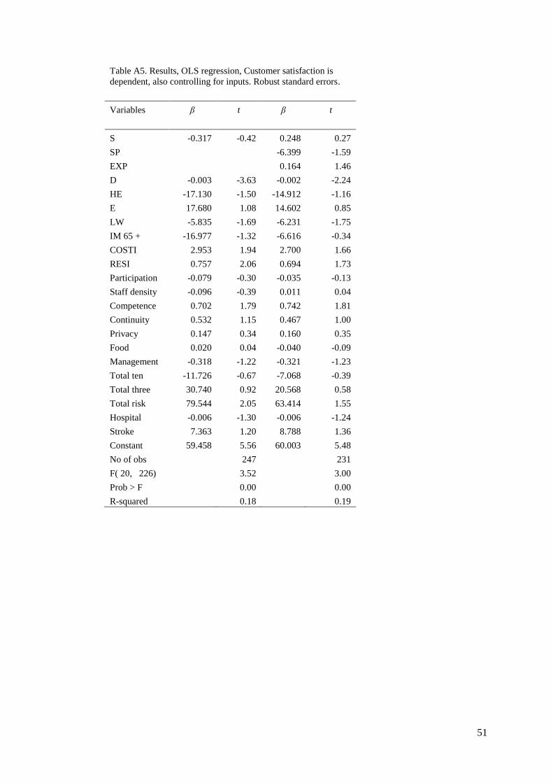
51

Table A5. Results, OLS regression, Customer satisfaction is

dependent, also controlling for inputs. Robust standard errors.

Variables β t β t

S -0.317 -0.42 0.248 0.27

SP

-6.399 -1.59

EXP

0.164 1.46

D -0.003 -3.63 -0.002 -2.24

HE -17.130 -1.50 -14.912 -1.16

E 17.680 1.08 14.602 0.85

LW -5.835 -1.69 -6.231 -1.75

IM 65 + -16.977 -1.32 -6.616 -0.34

COSTI 2.953 1.94 2.700 1.66

RESI 0.757 2.06 0.694 1.73

Participation -0.079 -0.30 -0.035 -0.13

Staff density -0.096 -0.39 0.011 0.04

Competence 0.702 1.79 0.742 1.81

Continuity 0.532 1.15 0.467 1.00

Privacy 0.147 0.34 0.160 0.35

Food 0.020 0.04 -0.040 -0.09

Management -0.318 -1.22 -0.321 -1.23

Total ten -11.726 -0.67 -7.068 -0.39

Total three 30.740 0.92 20.568 0.58

Total risk 79.544 2.05 63.414 1.55

Hospital -0.006 -1.30 -0.006 -1.24

Stroke 7.363 1.20 8.788 1.36

Constant 59.458 5.56 60.003 5.48

No of obs

247

231

F( 20, 226) 3.52

3.00

Prob > F

0.00

0.00

R-squared 0.18

0.19