Embed Size (px)
Citation preview

Pulse Sequences
Field trip: Tuesday, Feb 5th
• Hardware tour of VUIIIS Philips 3T • Meet here at regular class time (11.15) • Complete MRI screening form!
Chuck Nockowski Philips Service Engineer

Reminder: Project/Presentation • Pick a special topic of interest to you:
– Clinical (e.g., cancer, stroke, Alzheimer’s disease) – Technical (e.g., parallel imaging, k-space, novel acquisition) – Hardware (e.g., coils, gradients, radiofrequency transmission)
NOTE: if you are actively working on an imaging research project (Ph.D., etc.) you must choose something different from your thesis topic! I must approve all topics: just email or talk to me.
Prepare written report 10-20 pgs; double-spaced; font=12 pt; margins=1’’
Present summary to class 15 min (~10 slides)

What do we know so far about how MR imaging works?
• When we place a brain, body, etc. in MRI scanner, spins of protons on water molecules will align, on average, with the main magnetic field – Main field is in z-direction – This occurs due to Zeeman effect
• Lower energy state for alignment of spins with, vs. against, B0 z

What do we know so far about how MR imaging works?
• After magnetization (M) reaches equilibrium with main magnetic field B0 (few seconds), we can apply a rotating field B1 to cause M to move into the transverse (x-y) plane – Frequency of pulse given by ( γB ) – The duration of the pulse determines the “flip
angle” • e.g., if 5 ms pulse gives 45 degree flip angle • 10 ms pulse gives 90 degree flip angle

What do we know so far about how MR imaging works?
• If we turn off the B1 pulse, M will revert to its equilibrium orientation because of relaxation – Longitudinal component (Mz) re-aligns with z
according to time constant T1
– Transverse component (Mxy) decays to zero with time constant T2(*)
• T1 and T2 are (i) independent and (ii) unique for different tissue types. – Sources of two different contrasts in MRI!

What do we know so far about how MR imaging works?
• We detect oscillations from M by using a coil – Oscillating magnetic field will induce current in a coil – Faraday induction
• We discern spatial information from sample by: – Applying a gradient during signal acquisition
• This generates a spatially varying phase for the M vectors • (i.e., the gradient encodes spatial information)
– Perform Fourier transform of acquired signal to obtain estimate of spin density function (i.e., image) • Generally, we do this in 2-D and consider spatial frequencies.
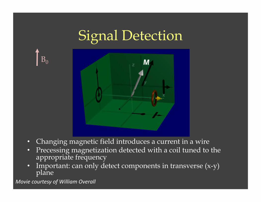
Signal Detection
• Changing magnetic field introduces a current in a wire • Precessing magnetization detected with a coil tuned to the
appropriate frequency • Important: can only detect components in transverse (x-y)
plane
B0
Movie courtesy of William Overall

Going further • We know basics of MRI physics, slice selection,
and image formation
• How do we use this information to generate contrast?
• How do we obtain T1, T2, T2*, diffusion, flow, etc. weightings?
• Need to understand pulse sequence variants and parameters
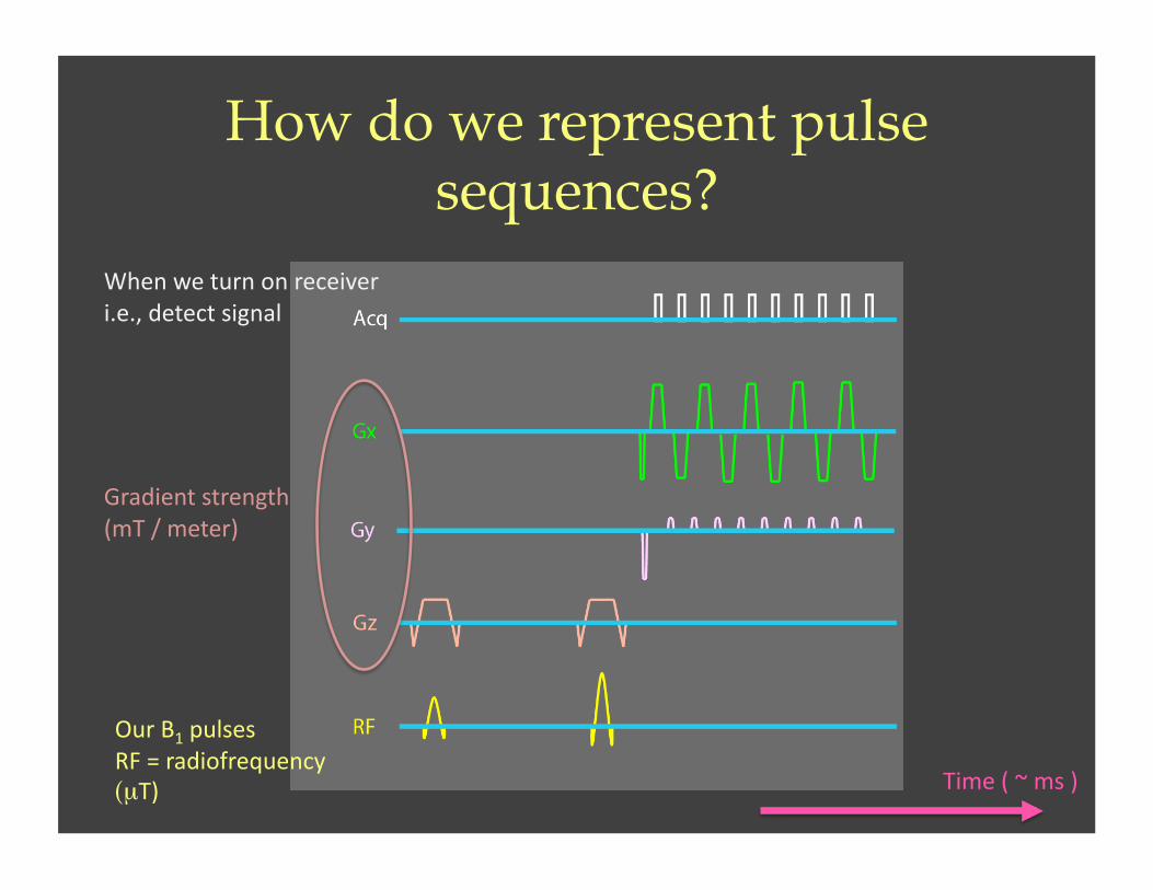
How do we represent pulse sequences?
Gradient strength (mT / meter)
When we turn on receiver i.e., detect signal
Our B1 pulses RF = radiofrequency (µT) Time ( ~ ms )
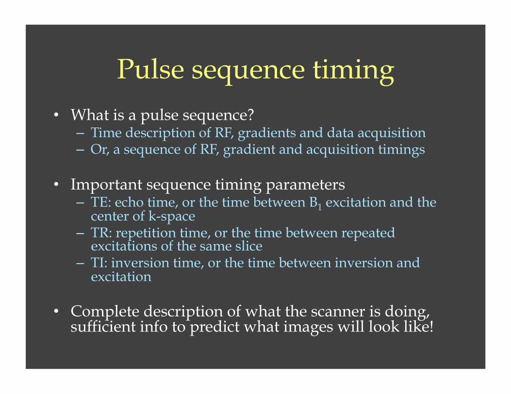
Pulse sequence timing • What is a pulse sequence?
– Time description of RF, gradients and data acquisition – Or, a sequence of RF, gradient and acquisition timings
• Important sequence timing parameters – TE: echo time, or the time between B1 excitation and the
center of k-space – TR: repetition time, or the time between repeated
excitations of the same slice – TI: inversion time, or the time between inversion and
excitation
• Complete description of what the scanner is doing, sufficient info to predict what images will look like!
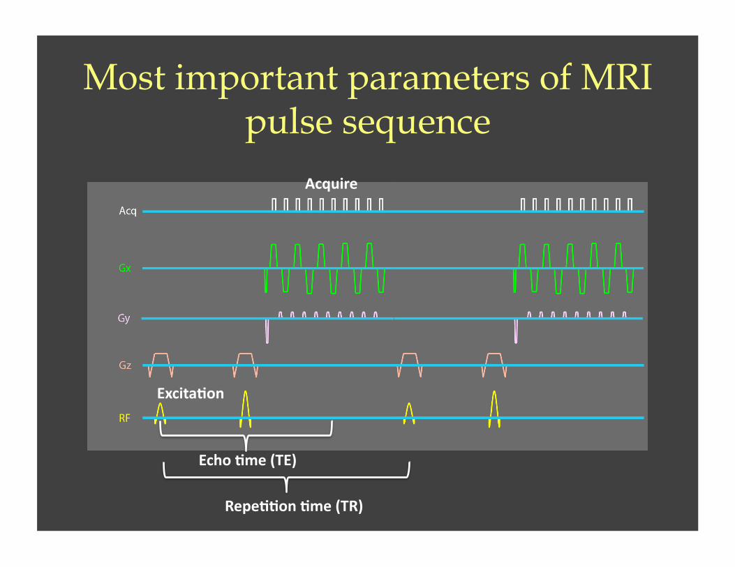
Most important parameters of MRI pulse sequence
Excita'on
Echo 'me (TE)
Acquire
Repe''on 'me (TR)

Introduction to pulse sequences
• What influences signal level? – Proton density, T1, T2, T2*
• Simple pulse sequences – Gradient echo, spin echo and inversion
recovery
• Readout trajectory and considerations – Bandwidth, SNR, artifacts, and time

Excitation
• Tip magnetization vector from being aligned with the magnetic field (B0) so that it is in the x-y (transverse) plane – Do this with radiofrequency (RF) “excitation”
pulse
• The flip angle of the RF excitation can be more or less than 90 degrees – So long as some magnetization is in
transverse plane

Excitation Pulse
Laboratory reference frame (e.g., sitting at the scanner console)
Movie courtesy of William Overall
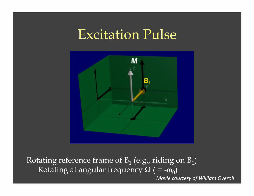
Excitation Pulse
Rotating reference frame of B1 (e.g., riding on B1) Rotating at angular frequency Ω ( = -ω0)
Movie courtesy of William Overall

Turn off the RF pulse
• Excitation pulse moves some component of the magnetization vector into the transverse plane
• After this, we turn off the RF pulse • The “excited” magnetization will relax back
to its original state – The speed of this relaxation is determined by two
time constants: • Transverse plane: T2 • Longitudinal plane: T1 • T2 and T1 are completely independent!

What happens after we turn off the RF excitation pulse?
Mz returns to alignment with main magnetic field T1 describes this relaxation time
Movie courtesy of William Overall
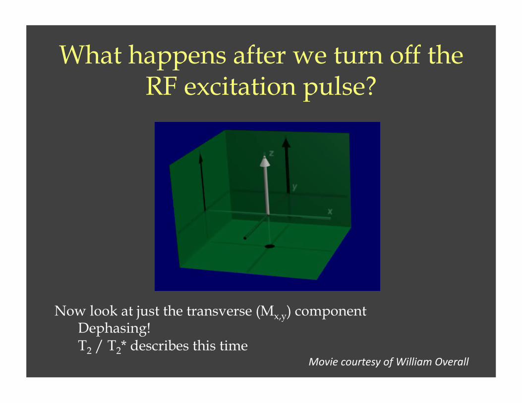
What happens after we turn off the RF excitation pulse?
Now look at just the transverse (Mx,y) component Dephasing! T2 / T2* describes this time
Movie courtesy of William Overall

Transverse magnetization
T2 = 25 ms T2 = 50 ms T2 = 100 ms
Mx,y = e-TE/T2

Longitudinal magnetization
T1 = 800 ms T1 = 1200 ms T1 = 4300 ms
Mz = 1-e-TR/T1
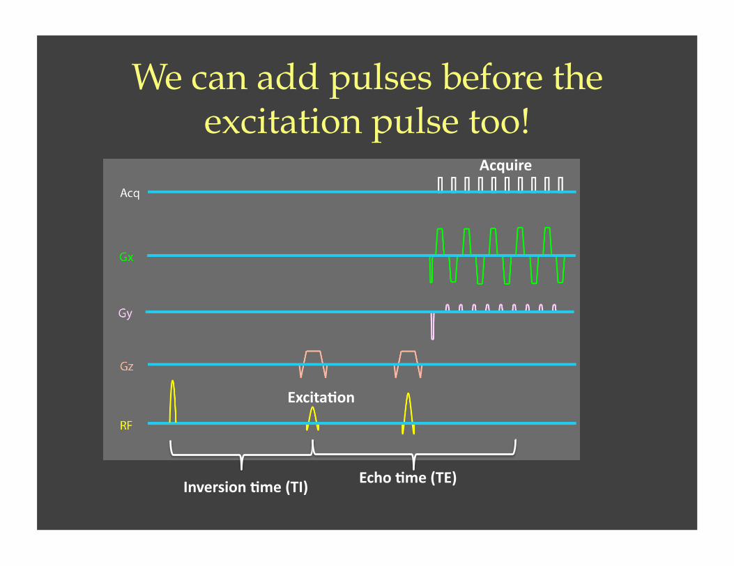
We can add pulses before the excitation pulse too!
Excita'on
Echo 'me (TE)
Acquire
Inversion 'me (TI)
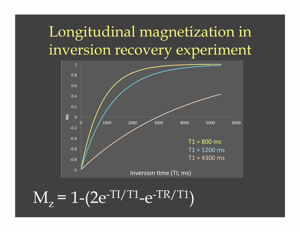
Longitudinal magnetization in inversion recovery experiment
T1 = 800 ms T1 = 1200 ms T1 = 4300 ms
Mz = 1-(2e-TI/T1-e-TR/T1)
Inversion Mme (TI; ms)

MRI signal
T1 = 800 ms T1 = 1200 ms T1 = 4300 ms
T2 = 25 ms T2 = 50 ms T2 = 100 ms
Signal ~ C Mx,y(TE) Mz(TR,TI)
Water density Specific to tissue We don’t change this
Transverse magnetization Manipulate magnitude by varying TE
Longitudinal magnetization Manipulate magnitude by varying TR

What are T1 and T2 values? • Depends on field strength. T1 increases with field strength whereas
T2 decreases with field strength
• T2 times at 3 Tesla – White matter ~ 110 ms – Gray matter ~ 80 ms – Cerebrospinal fluid ~ 600 ms
• T1 times at 3 Tesla – White matter ~ 800 ms – Gray matter ~ 1200 ms – Cerebrospinal fluid ~ 4300 ms
• Unique T1/T2 for other tissue types as well (e.g., tumor, blood, edema, etc.) – Unique T1/T2 provides contrast between tissues – More to come on this next week!

One additional relaxation time: T2*
• Dephasing of spins in transverse plane causes magnetization vectors to oppose each other. – Net signal is lower due to dephasing – Leads to apparent decrease in T2.
• This is called effective T2, or T2* • T2’ = relaxation due to field inhomogeneity
€
1T2* =
1T2' +
1T2

Relaxation times thus far
• T1: relaxation time in longitudinal plane • T2*: effective relaxation time in transverse
plane. – Includes dephasing from controllable
inhomogeneities (e.g., imperfect scanner shielding, magnetic objects/implants, etc.)
– Also includes dephasing from uncontrollable interactions (e.g., local interactions of molecules in voxel)
• T2: Relaxation time in transverse plane only from uncontrollable “spin-spin” effects

How can we obtain T2 and/or T2* contrast?
• Gradient echo (GRE): Fundamentally T2*-weighted
• Spin echo (SE): Fundamentally T2-weighted
• Note: we can vary pulse sequence parameters to make these sequences T1-weighted instead (more to come on this next time)

Fundamentals of gradient echo (GRE)
• What does signal look like after the excitation?
RF
Signal
Free induction decay (FID) Well-defined frequency (Modulated by decaying exponential)

Gradient echo (GRE) pulse sequence
Vendor-speak
Philips: Fast Field Echo (FFE) Siemens: Fast Low Angle Shot (FLASH) GE: SPoiled Gradient Recall (SPGR)
• Gradient echo can be used with different k-space trajectories – e.g., GRE spinwarp, GRE spiral, GRE radial
• Many structural, fMRI, susceptibility scans utilize GRE contrast

Fundamentals of gradient echo (GRE)
• Apply Gx gradient with half the area sequentially with slice-select gradient – Causes an “echo”: spins within the slice will
be in-phase at time TE
RF
Gz
Signal TE
Gx
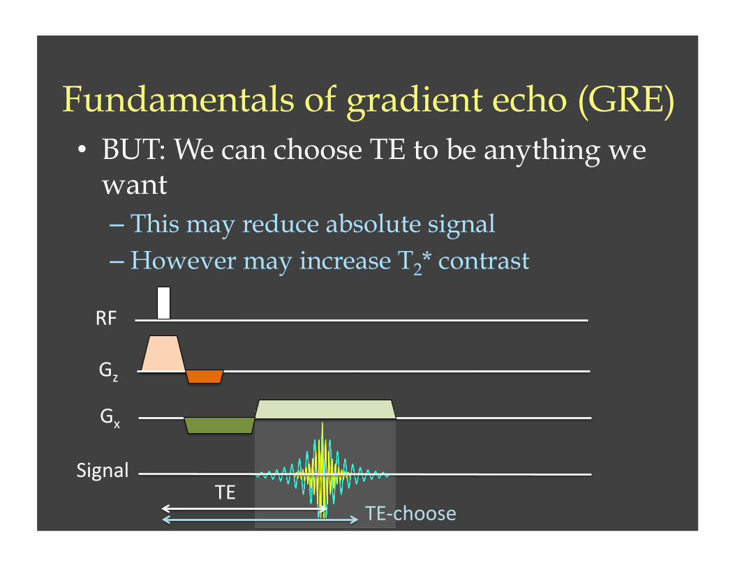
Fundamentals of gradient echo (GRE) • BUT: We can choose TE to be anything we
want – This may reduce absolute signal – However may increase T2* contrast
TE-‐choose
RF
Gz
Signal TE
Gx

Fundamentals of gradient echo (GRE) • Optimum TE has most signal • TE-choose has most contrast! – Best choice may depend on application – BOLD fMRI: choose TE to maximize contrast in
and around venous blood water
TE-‐choose
RF
Gz
Signal TE
Gx

Problem: dephasing of spins quite short, especially at high field
• At 7 Tesla, venous blood water T2* < 5 ms
• At 7 Tesla, tissue water T2* ~ 25 ms
• At 3 Tesla, these numbers are longer (15 – 40 ms)
• Difficult to fill our k-space when the signal decays so quickly. Can we do better?

Can we do anything to lengthen the time it takes for spins to dephase?
• Yes, apply an RF pulse to transverse magnetization
Movie courtesy of William Overall
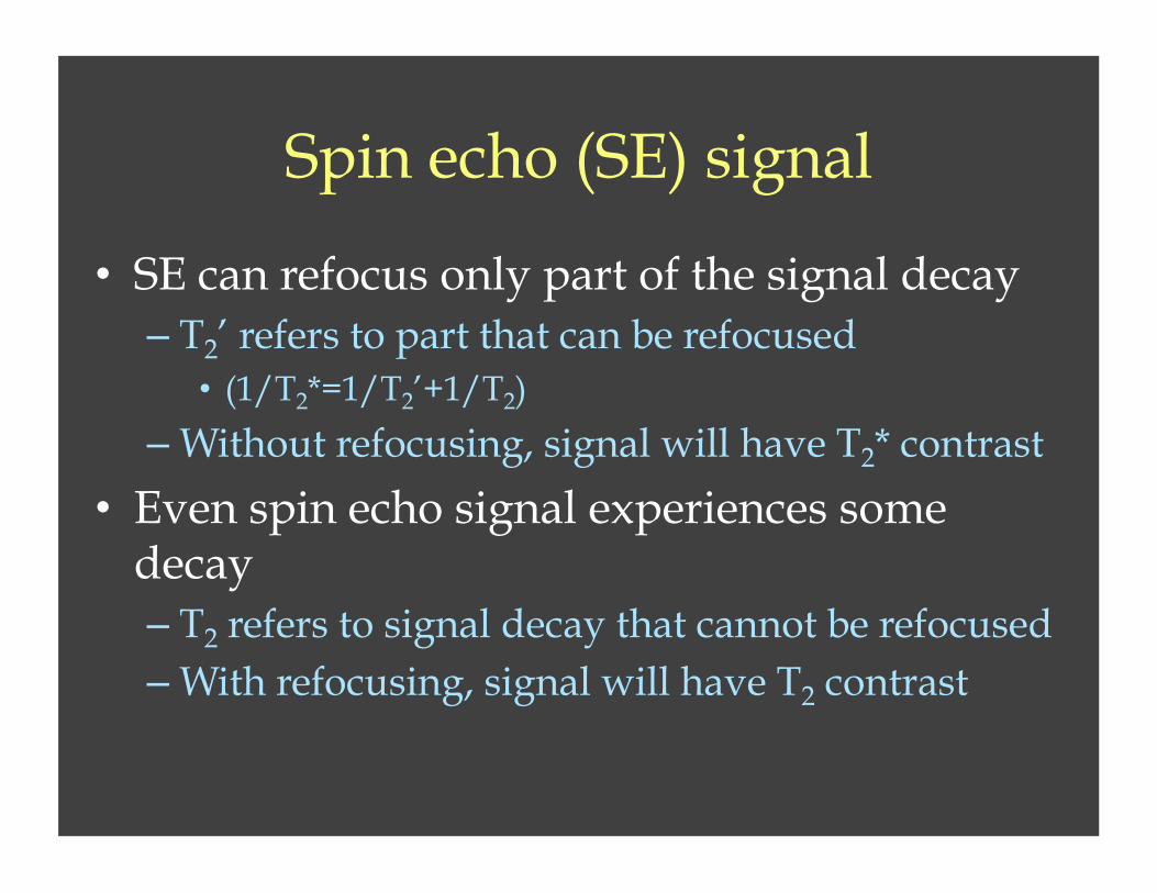
Spin echo (SE) signal
• SE can refocus only part of the signal decay – T2’ refers to part that can be refocused
• (1/T2*=1/T2’+1/T2)
– Without refocusing, signal will have T2* contrast
• Even spin echo signal experiences some decay – T2 refers to signal decay that cannot be refocused – With refocusing, signal will have T2 contrast

T2* < T2

Gradient vs. spin echo sequences
Gradient echo (GRE) T2* decay Fast!
Spin echo (SE) T2 decay T2 > T2*

Gradient and spin echo sequences can have different k-space readout trajectories
Cartesian Spiral

Examples of different MRI sequences
• Gradient echo (T2*-weighted depending on TE) – Blood oxygenation level-dependent (BOLD)
functional MRI (fMRI) – Susceptibility weighted imaging
• Spin echo (T2-weighted depending on TE) – Fluid attenuated inversion recovery (FLAIR) – Diffusion weighted imaging
• Inversion recovery (inversion prepulse followed by GRE or SE) – FLAIR – Arterial spin labeling (ASL) – Vascular space occupancy (VASO)

Introduction to pulse sequences
• Basic image contrast – Proton density, T1, T2, T2*
• Simple pulse sequences – Gradient echo and spin echo
• Readout trajectory and considerations – Bandwidth – Signal-to-noise ratio (SNR)
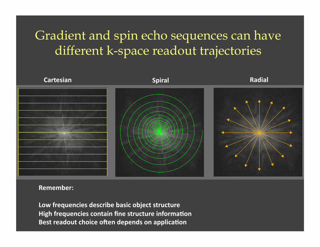
Gradient and spin echo sequences can have different k-space readout trajectories
Cartesian Radial Spiral
Remember:
Low frequencies describe basic object structure High frequencies contain fine structure informa'on Best readout choice oOen depends on applica'on
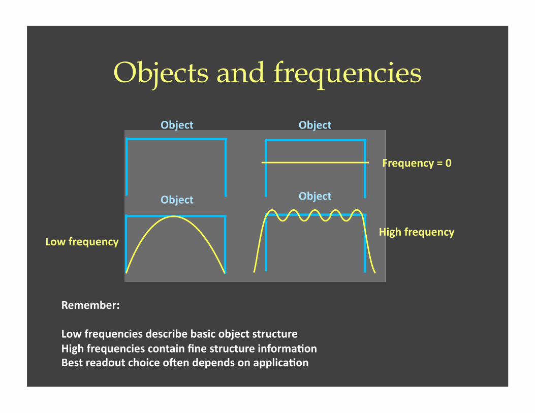
Objects and frequencies
Object
Frequency = 0
Low frequency High frequency
Remember:
Low frequencies describe basic object structure High frequencies contain fine structure informa'on Best readout choice oOen depends on applica'on
Object
Object Object

Frequencies in images
High frequency Low frequency
Low frequency
High frequency
Cornelius Vanderbilt 1794-‐1877
Signal to noise ratio (SNR) • Image quality frequency evaluated in terms of signal-
to-noise ratio (SNR) • SNR: signal / noise (σ) • Signal is easy to characterize: just the net signal we
detect • Noise is more difficult, with multiple contributions:
– Thermal noise: noise due to hardware, outside RF interference, etc.
– Physiological “noise”: fluctuations secondary to biological changes (e.g., cardiac fluctuations, respiratory fluctuations, “spontaneous” brain activity
– Should keep track of which noise you are interested in
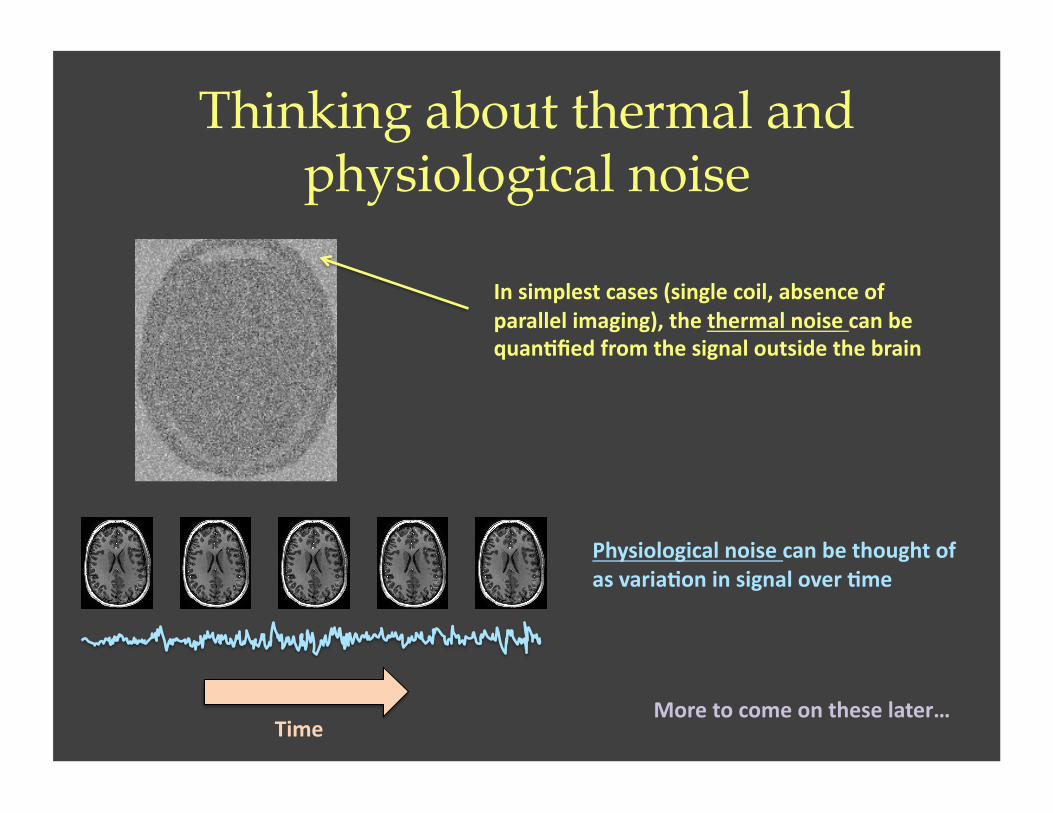
Thinking about thermal and physiological noise
In simplest cases (single coil, absence of parallel imaging), the thermal noise can be quan'fied from the signal outside the brain
Time
Physiological noise can be thought of as varia'on in signal over 'me
More to come on these later…

What influences SNR? Voxel size
1 x 1 x 1 mm Volume = 1 mm3
2 x 2 x 1 mm Volume = 4 mm3
• Larger voxels have signal contribution from more spins – Signal proportional to voxel
volume
– Note: reducing voxel size by n along each m dimensions costs nm in signal
– For example, changing from 1x1x1 mm to 2x2x1 mm increases signal by four-fold
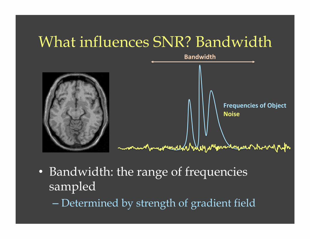
What influences SNR? Bandwidth
• Bandwidth: the range of frequencies sampled – Determined by strength of gradient field
Frequencies of Object Noise
Bandwidth

What influences SNR? Bandwidth
• High bandwidth = high noise • Low bandwidth = low noise
Frequencies of Object Noise
Bandwidth

Bandwidth and the readout Tshot
Tshot
Gradient Strength
Increasing the readout bandwidth reduces total time required to obtain signal (Tshot ~ 1/Gx)
Gx
Gx

What influences SNR? Multiple acquisitions
• Each time additional measurement is acquired, signal adds but random noise does not – Each line in multi-line readout – Every plane in 3D acquisition – Any repetition or averaging of acquisition
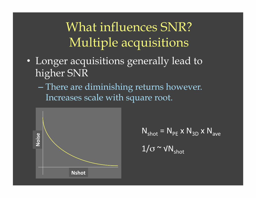
• Longer acquisitions generally lead to higher SNR – There are diminishing returns however.
Increases scale with square root.
Nshot
Noise Nshot = NPE x N3D x Nave
1/σ ~ √Nshot
What influences SNR? Multiple acquisitions

• Good rule of thumb: SNR is higher for longer scan times – For multi-shot acquisitions, where multiple
excitations and readouts are used to acquire a single slice of data, the total time time (Ttot) is the product of the number of shots (Nshot) and the time of each shot (Tshot):
– Ttot = Nshot x Tshot
1/σ ~ √[Nshot x Tshot] = √TTot
What influences SNR? Imaging time
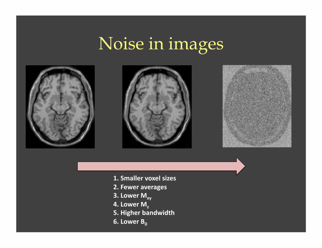
Noise in images
1. Smaller voxel sizes 2. Fewer averages 3. Lower Mxy
4. Lower Mz 5. Higher bandwidth 6. Lower B0
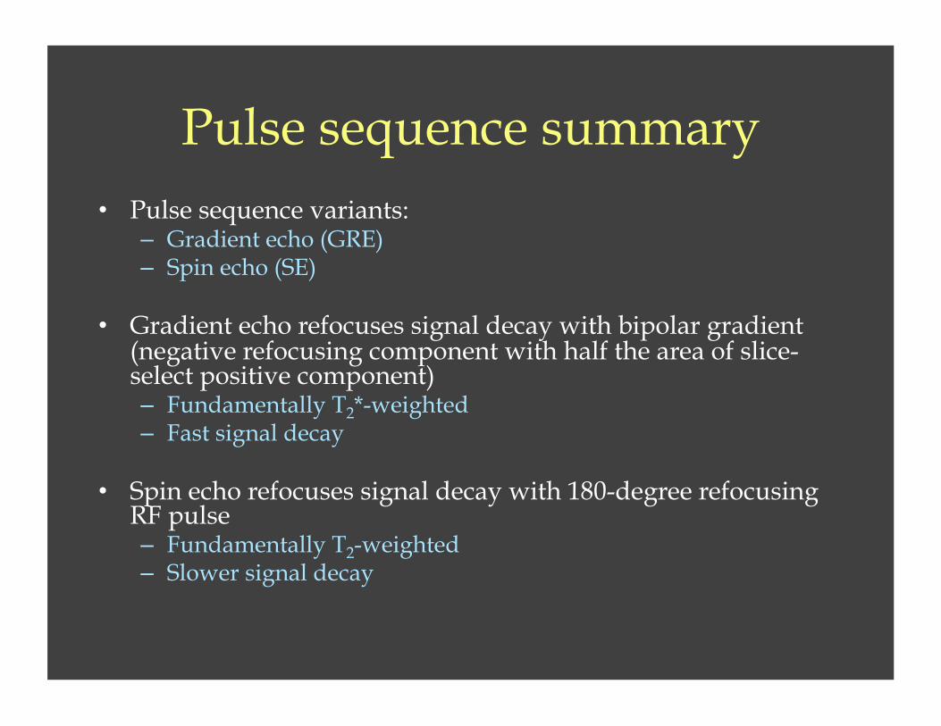
Pulse sequence summary • Pulse sequence variants:
– Gradient echo (GRE) – Spin echo (SE)
• Gradient echo refocuses signal decay with bipolar gradient (negative refocusing component with half the area of slice-select positive component) – Fundamentally T2*-weighted – Fast signal decay
• Spin echo refocuses signal decay with 180-degree refocusing RF pulse – Fundamentally T2-weighted – Slower signal decay

Pulse sequence summary
Excita'on
Echo 'me (TE)
Acquire
Repe''on 'me (TR)

Noise in images
1. Smaller voxel sizes 2. Fewer averages 3. Lower Mxy
4. Lower Mz 5. Higher bandwidth 6. Lower B0
Coming up… • Thursday: Contrast manipulation + example
problems • Tuesday: Jay Moore: RF pulses / hardware • Thursday: Jay Moore: RF pulses / hardware • Tuesday: Chuck Nockowski: Hardware tour
• Mid-term exam: 19 Feb (not 14 Feb)