Eindhoven University of Technology

MASTER

Two-dimensional pattern matching

van de Rijdt, M.G.W.H.

Award date:2005

DisclaimerThis document contains a student thesis (bachelor's or master's), as authored by a student at Eindhoven University of Technology. Studenttheses are made available in the TU/e repository upon obtaining the required degree. The grade received is not published on the documentas presented in the repository. The required complexity or quality of research of student theses may vary by program, and the requiredminimum study period may vary in duration.

General rightsCopyright and moral rights for the publications made accessible in the public portal are retained by the authors and/or other copyright ownersand it is a condition of accessing publications that users recognise and abide by the legal requirements associated with these rights.

• Users may download and print one copy of any publication from the public portal for the purpose of private study or research. • You may not further distribute the material or use it for any profit-making activity or commercial gain

Take down policyIf you believe that this document breaches copyright please contact us providing details, and we will remove access to the work immediatelyand investigate your claim.

Download date: 28. Aug. 2018

TECHNISCHE UNIVERSITEIT EINDHOVEN

Department of Mathematics and Computer Science

MASTER’S THESIS

Two-dimensional pattern matching

byM.G.W.H. van de Rijdt

Supervisors: dr. ir. G. Zwaanprof. dr. B.W. Watson

Eindhoven, August 2005

1

Abstract

This thesis contains formal derivations of several two-dimensional pattern matching algorithms.

The two-dimensional pattern matching problem is to find all exact occurrences of a given two-dimensional pattern matrix within a larger matrix. Two-dimensional pattern matching is mostlyapplied in image processing (and image recognition in particular), although there are other appli-cations as well.

We give a formal derivation (and correctness proof) for several known algorithms in this field, aswell as a few improvements to some of these algorithms.

Samenvatting

Dit afstudeerverslag bevat formele afleidingen voor enige algoritmen voor twee-dimensionale pa-troonherkenning.

Het probleem van twee-dimensionale patroonherkenning bestaat uit het vinden van de voorkomensvan een gegeven twee-dimensionale patroonmatrix binnen een grotere matrix. Twee-dimensionalepatroonherkenning wordt vooral toegepast binnen de beeldverwerking (en in het bijzonder beeld-herkenning), maar er zijn ook andere toepassingen.

We geven een formele afleiding (tevens correctheidsbewijs) van verschillende bekende algoritmendie dit probleem oplossen. Daarnaast introduceren we enige verbeteringen op sommige van dezealgoritmen.

2

3

Preface

This document is my Master’s Thesis, written to complete my education in “Technische Informa-tica” (Technical Computer Science). It is the result of my research for the Software Constructiongroup at the Department of Mathematics and Computer Science at the Eindhoven University ofTechnology (TU/e), under the supervision of dr. ir. Gerard Zwaan and prof. dr. Bruce Watson.

I thank Bruce Watson, for initially suggesting the topic of two-dimensional pattern matching andinvolving me in the FASTAR (Finite Automata Systems – Theoretical and Applied Research)group. I would also like to thank Gerard Zwaan, for his reviews of countless draft versions of thisthesis and offering many corrections and suggestions to improve this document greatly. I thankLoek Cleophas for his reviews of several early versions of this dcument, as well as some pointersto relevant articles. Many thanks go to my good friend Remi Bosman, for all the brainstormingand his reviews of this document’s near-final drafts. I thank LaQuSo (the Laboratory for QualitySoftware at the TU/e), for providing me with a workspace for many months. Finally, I would liketo thank my friends and family, particularly my parents, for all their support during the time ofthis research.

– Martijn van de Rijdt, August 2005.

4

5

Contents

0 Introduction 10

1 Preliminaries 12

1.0 Two-dimensional arrays . . . . . . . . . . . . . . . . . . . . . . . . . . . . . . . . . 12

1.1 Composed matrices . . . . . . . . . . . . . . . . . . . . . . . . . . . . . . . . . . . . 13

1.2 One-dimensional pattern matching . . . . . . . . . . . . . . . . . . . . . . . . . . . 14

2 Problem 16

3 Naive algorithm 18

3.0 Algorithm structure . . . . . . . . . . . . . . . . . . . . . . . . . . . . . . . . . . . 18

3.1 Match function . . . . . . . . . . . . . . . . . . . . . . . . . . . . . . . . . . . . . . 18

4 Filter-based approach 20

4.0 The filter function . . . . . . . . . . . . . . . . . . . . . . . . . . . . . . . . . . . . 20

4.1 One-dimensional pattern matching in one direction . . . . . . . . . . . . . . . . . . 21

4.2 Efficient computation and storage of the reduced text . . . . . . . . . . . . . . . . 22

4.3 Baker and Bird . . . . . . . . . . . . . . . . . . . . . . . . . . . . . . . . . . . . . . 23

4.4 Takaoka and Zhu . . . . . . . . . . . . . . . . . . . . . . . . . . . . . . . . . . . . . 26

4.5 Generalisations . . . . . . . . . . . . . . . . . . . . . . . . . . . . . . . . . . . . . . 30

5 Baeza-Yates and Regnier 32

5.0 Algorithm structure . . . . . . . . . . . . . . . . . . . . . . . . . . . . . . . . . . . 32

5.1 Baeza-Yates and Regnier’s CheckMatch approach . . . . . . . . . . . . . . . . . . . 33

5.2 Inspecting fewer pattern rows . . . . . . . . . . . . . . . . . . . . . . . . . . . . . . 36

5.3 Inspecting only matching pattern rows . . . . . . . . . . . . . . . . . . . . . . . . . 39

5.4 Computation of unique row indices . . . . . . . . . . . . . . . . . . . . . . . . . . . 44

5.5 Generalisations . . . . . . . . . . . . . . . . . . . . . . . . . . . . . . . . . . . . . . 44

6 Polcar 48

6.0 Introduction . . . . . . . . . . . . . . . . . . . . . . . . . . . . . . . . . . . . . . . . 48

6.1 Derivation . . . . . . . . . . . . . . . . . . . . . . . . . . . . . . . . . . . . . . . . . 48

6.2 Algorithm structure . . . . . . . . . . . . . . . . . . . . . . . . . . . . . . . . . . . 54

6

6.3 Precomputation . . . . . . . . . . . . . . . . . . . . . . . . . . . . . . . . . . . . . . 56

6.3.0 Representing sets of matrices by lists of maximal elements . . . . . . . . . . 56

6.3.1 Precomputation algorithm structure . . . . . . . . . . . . . . . . . . . . . . 61

6.3.2 Case analysis . . . . . . . . . . . . . . . . . . . . . . . . . . . . . . . . . . . 63

6.3.3 Entire precomputation algorithm . . . . . . . . . . . . . . . . . . . . . . . . 79

6.3.4 Computation of the “failure function” . . . . . . . . . . . . . . . . . . . . . 81

6.4 Entire algorithm . . . . . . . . . . . . . . . . . . . . . . . . . . . . . . . . . . . . . 85

6.5 Remarks . . . . . . . . . . . . . . . . . . . . . . . . . . . . . . . . . . . . . . . . . . 86

7 Conclusions and future work 88

7.0 Conclusions . . . . . . . . . . . . . . . . . . . . . . . . . . . . . . . . . . . . . . . . 88

7.1 Future work . . . . . . . . . . . . . . . . . . . . . . . . . . . . . . . . . . . . . . . . 88

A Properties of div and mod 90

B Properties of pref and suff (for strings) 92

C Properties of pref and suff (for matrices) 94

D Lists 96

7

List of Figures

0 A two-dimensional array . . . . . . . . . . . . . . . . . . . . . . . . . . . . . . . . . 12

1 Every match intersects with a row i ∗m1 − 1 . . . . . . . . . . . . . . . . . . . . . 32

2 Submatrix of the text, inspected when a match occurs in row i ∗m1 − 1 . . . . . . 35

3 The Baeza-Yates algorithm idea, applied in three dimensions . . . . . . . . . . . . 45

4 A pattern occurrence as a suffix of a prefix of the text . . . . . . . . . . . . . . . . 48

8

9

0 Introduction

In this text we will formally derive a number of known two-dimensional pattern matching algo-rithms. The two-dimensional pattern matching problem consists of finding all occurrences of agiven two-dimensional matrix, the so-called pattern, in a larger two-dimensional matrix, the text.

We provide formal derivations of these algorithms for a number of reasons. First of all, a formalderivation is also a correctness proof. This method also ensures that all algorithms are presentedin a (more-or-less) uniform way, which is independant of implementation details and choice ofprogramming language. And finally, this presentation also highlights the major design decisionsduring the algorithm’s construction. Variations on these decisions may give rise to new solutionsto the two-dimensional pattern matching problem.

Part of the original goal of this research was to construct a taxonomy of algorithms. A taxonomy isa structured classification of algorithms – see for examples [Wat95, WZ92, WZ93, WZ95, WZ96].However, as we will see, the differences between most of the algorithms discussed here are sogreat, that the corresponding taxonomy would have a very coarse structure and therefore wouldnot provide much additional value.

Section 1 introduces some definitions and notations used in the rest of the thesis. In section 2,we formally define the two-dimensional pattern matching problem. Section 3 contains a descrip-tion of a very straightforward, but inefficient, solution to the problem: the naive algorithm. Insection 4 the so-called filter-based approaches are discussed; most notably: Baker and Bird’s al-gorithm ([Bak78, Bir77]) and Takaoka and Zhu’s algorithm ([TZ89, TZ94]). Section 5 containsthe description of Baeza-Yates and Regnier’s algorithm ([BYR93]) and in section 6 we will derivePolcar’s algorithm ([Pol04, MP04]). Section 7 will contain the conclusions and suggestions forfuture work. Finally, in the appendices we list some definitions, notations and properties that areuseful in the derivations in the main text, but not an essential part of the derivations themselves.

10

11

1 Preliminaries

1.0 Two-dimensional arrays

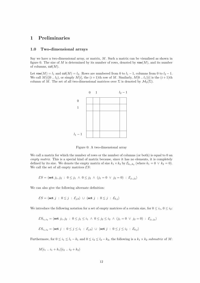
Say we have a two-dimensional array, or matrix, M . Such a matrix can be visualised as shown infigure 0. The size of M is determined by its number of rows, denoted by row(M), and its numberof columns, col(M).

Let row(M) = l1 and col(M) = l2. Rows are numbered from 0 to l1− 1, columns from 0 to l2 − 1.We call M [i][0 .. l2), or simply M [i], the (i+1)th row of M . Similarly, M [0 .. l1)[i] is the (i+1)thcolumn of M . The set of all two-dimensional matrices over Σ is denoted by M2(Σ).

0

1

l1 − 1

0 1 l2 − 1

Figure 0: A two-dimensional array

We call a matrix for which the number of rows or the number of columns (or both) is equal to 0 anempty matrix. This is a special kind of matrix because, since it has no elements, it is completelydefined by its size. We denote the empty matrix of size k1×k2 by Ek1,k2 (where k1 = 0 ∨ k2 = 0).We call the set of all empty matrices ES:

ES = 〈set j1, j2 : 0 ≤ j1 ∧ 0 ≤ j2 ∧ (j1 = 0 ∨ j2 = 0) : Ej1,j2〉

We can also give the following alternate definition:

ES = 〈set j : 0 ≤ j : Ej,0〉 ∪ 〈set j : 0 ≤ j : E0,j〉

We introduce the following notation for a set of empty matrices of a certain size, for 0 ≤ i1, 0 ≤ i2:

ESi1,i2 = 〈set j1, j2 : 0 ≤ j1 ≤ i1 ∧ 0 ≤ j2 ≤ i2 ∧ (j1 = 0 ∨ j2 = 0) : Ej1,j2〉

ESi1,i2 = 〈set j : 0 ≤ j ≤ i1 : Ej,0〉 ∪ 〈set j : 0 ≤ j ≤ i2 : E0,j〉

Furthermore, for 0 ≤ i1 ≤ l1 − k1 and 0 ≤ i2 ≤ l2 − k2, the following is a k1 × k2 submatrix of M :

M [i1 .. i1 + k1)[i2 .. i2 + k2)

12

For 0 ≤ j1 < k1 and 0 ≤ j2 < k2:

(M [i1 .. i1 + k1)[i2 .. i2 + k2))[j1, j2] = M [i1 + j1, i2 + j2]

If i1 and i2 are both equal to 0, we call the submatrix a prefix of M . If i1+k1 = l1 and i2+k2 = l2,we call the submatrix a suffix of M . More formally, a prefix of M is an element of the set pref(M).A suffix is an element of suff(M). We define the sets pref(M) and suff(M) similarly to the one-dimensional case:

pref(M) = 〈set i1, i2 : 0 ≤ i1 ≤ l1 ∧ 0 ≤ i2 ≤ l2 : M [0 .. i1)[0 .. i2)〉suff(M) = 〈set i1, i2 : 0 ≤ i1 ≤ l1 ∧ 0 ≤ i2 ≤ l2 : M [i1 .. l1)[i2 .. l2)〉

Note that both pref(M) and suff(M) include the following empty matrices: ESl1,l2 .

Two matrices M and N are equal if they have the same size, say k1 × k2, and:

〈∀h1, h2 : 0 ≤ h1 < k1 ∧ 0 ≤ h2 < k2 : M [h1, h2] = N [h1, h2]〉

1.1 Composed matrices

Suppose we have l1∗l2 matrices, called Mi1,i2 (0 ≤ i1 < l1 and 0 ≤ i2 < l2), for which the followingholds:

〈∀i1, i2 : 0 ≤ i1 < l1 ∧ 0 ≤ i2 < l2 : row(Mi1,i2) = row(Mi1,0) ∧ col(Mi1,i2) = col(M0,i2)〉

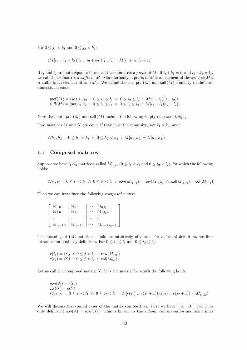
Then we can introduce the following composed matrix :

M0,0 M0,1 · · · M0,l2−1

M1,0 M1,1 · · · M1,l2−1

......

. . ....

Ml1−1,0 Ml1−1,1 · · · Ml1−1,l2−1

The meaning of this notation should be intuitively obvious. For a formal definition, we firstintroduce an auxiliary definition. For 0 ≤ i1 ≤ l1 and 0 ≤ i2 ≤ l2:

r(i1) = 〈Σj : 0 ≤ j < i1 : row(Mj,0)〉c(i2) = 〈Σj : 0 ≤ j < i2 : col(M0,j)〉

Let us call the composed matrix N . It is the matrix for which the following holds:

row(N) = r(l1)col(N) = c(l2)〈∀j1, j2 : 0 ≤ j1 < l1 ∧ 0 ≤ j2 < l2 : N [r(j1) .. r(j1 + 1))[c(j2) .. c(j2 + 1)) = Mj1,j2〉

We will discuss two special cases of the matrix composition. First we have[

A B]

(which isonly defined if row(A) = row(B)). This is known as the column concatenation and sometimes

13

written as A�B or [A B]. The other special case is[

AB

](only defined if col(A) = col(B)): the

row concatenation, which is sometimes denoted in the literature by A � B or [A; B]. For a moreextensive description of row and column concatenation and how these two operators can be usedto define two-dimensional regular expressions and two-dimensional languages, we refer to [RS97].

Using the matrix composition, we can give an alternate definition for pref and suff, which isequivalent to the defintions given in section 1.0, but expressed in terms of the matrix composition,as opposed to indices:

pref(M) = 〈set A, B,C, D : M =[

A BC D

]: A〉

suff(M) = 〈set A, B,C, D : M =[

A BC D

]: D〉

1.2 One-dimensional pattern matching

In some of the two-dimensional pattern matching algorithms to be discussed, we will use a one-dimensional pattern matching algorithm (for example, on rows or columns of the text). Whenit is not relevant which one-dimensional pattern matching algorithm is used, we will refer tofunction PM1, with the following specification (for strings p and t):

PM1(p, t) = 〈set l, r : t = lpr : |l|〉

In the same spirit we introduce the multipattern matching function MPM1, with the followingspecification (for set of strings PS and string t):

MPM1(PS, t) = 〈set l, p, r : p ∈ PS ∧ t = lpr : (|l|, p)〉

14

15

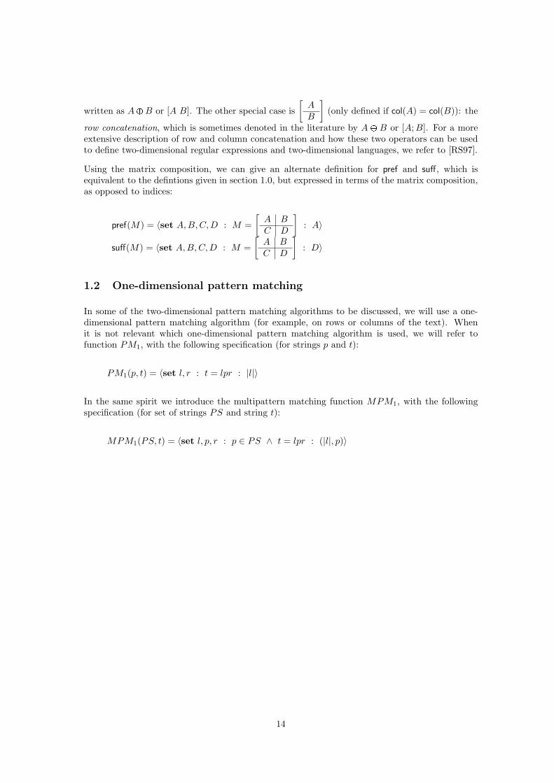
2 Problem

In ‘normal’ (one-dimensional) pattern matching, the problem is to find all occurrences of a pat-tern p in a text t, where both p and t are strings over an alphabet Σ. In the two-dimensional case,instead of matching strings, we are matching two-dimensional arrays.

Our pattern P and text T are matrices over Σ, with row(P ) = m1, col(P ) = m2, row(T ) = n1

and col(T ) = n2. In practical applications, the text is often a picture. However, we continue usingthe term ‘text’ in this overview to emphasise the similarities to one-dimensional pattern matching.

The problem is to find all exact matches of pattern P in text T . More formally, our postconditionis

R : O = 〈set i1, i2 : 0 ≤ i1 ≤ n1 −m1 ∧ 0 ≤ i2 ≤ n2 −m2 ∧T [i1 .. i1 + m1)[i2 .. i2 + m2) = P : (i1, i2)〉

Note that we identify occurrences of the pattern by their “upper-left corner”. Since the problemwe are focussing on is exact two-dimensional pattern matching, the size of each occurrence isthe same and equal to the size of the pattern. Therefore, any point can be used to representan occurrence. We have chosen the “upper left corner” because it is convenient for most of thealgorithms we will discuss, but we could have just as easily reported the “lower-right corner”, orany other point, instead.

16

17

3 Naive algorithm

3.0 Algorithm structure

The simplest way of establishing R is by checking, for all positions (i1, i2) in the text, whetherthere is a match starting at that position.

We introduce a set of index pairs D : N× N. We will maintain the following invariant:

P0 : O = 〈set i1, i2 : (i1, i2) ∈ D ∧ T [i1 .. i1 + m1)[i2 .. i2 + m2) = P : (i1, i2)〉

Invariant P0 is trivially established by the assignment O, D := ?,?. We have established R when:

D = [0, n1 −m1]× [0, n2 −m2]

Ad P0(D := D ∪ {(j1, j2)}):

〈set i1, i2 : (i1, i2) ∈ D ∪ {(j1, j2)} ∧ T [i1 .. i1 + m1)[i2 .. i2 + m2) = P : (i1, i2)〉= { split off (i1, i2) = (j1, j2), P0 }{

O ∪ {(j1, j2)} if T [j1 .. j1 + m1)[j2 .. j2 + m2) = PO if T [j1 .. j1 + m1)[j2 .. j2 + m2) 6= P

= { •matchT,P (i1, i2) ≡ T [i1 .. i1 + m1)[i2 .. i2 + m2) = P }{O ∪ {(j1, j2)} if matchT,P (j1, j2)O if ¬matchT,P (j1, j2)

Now we can give the so-called “naive algorithm”:

O,D := ?,?;for j1, j2 : 0 ≤ j1 ≤ n1 −m1 ∧ 0 ≤ j2 ≤ n2 −m2 → { inv. P0 }

if matchT,P (j1, j2) → O := O ∪ {(j1, j2)}[] ¬matchT,P (j1, j2) → skipfi;D := D ∪ {(j1, j2)}

rof

Note that the assignments to set D can be removed from the algorithm without harming itscorrectness; D is never inspected.

3.1 Match function

Recall our specification of matchT,P :

matchT,P (i1, i2) ≡ T [i1 .. i1 + m1)[i2 .. i2 + m2) = P

Again, we introduce a set of index pairs, C : N× N. We will maintain the following invariant:

Q0 : res ≡ 〈∀j1, j2 : (j1, j2) ∈ C : T [i1 + j1, i2 + j2] = P [j1, j2]〉

18

Invariant Q0 is initially trivially established by res, C := true,?. When the following holds, wehave established res = matchT,P (i1, i2):

C = [0, m1〉 × [0,m2〉

Ad Q0(C := C ∪ {(k1, k2)}):

〈∀j1, j2 : (j1, j2) ∈ C ∪ {(k1, k2)} : T [i1 + j1, i2 + j2] = P [j1, j2]〉≡ { split off (j1, j2) = (k1, k2), Q0 }

res ∧ T [i1 + k1, i2 + k2] = P [k1, k2]

The complete implementation becomes the following:

func matchT,P (i1, i2 :integer) :boolean{ pre: 0 ≤ i1 ≤ n1 −m1 ∧ 0 ≤ i2 ≤ n2 −m2 }{ result: T [i1 .. i1 + m1)[i2 .. i2 + m2) = P }|[

res, C := true,?;for k1, k2 : 0 ≤ k1 < m1 ∧ 0 ≤ k2 < m2 →

res := res ∧ T [i1 + k1, i2 + k2] = P [k1, k2];C := C ∪ {(k1, k2)}

rof ;return(res)

]|

Note that we can improve on this algorithm: we can stop the computation as soon as res becomesfalse. We can also omit set C, since it is never inspected.

19

4 Filter-based approach

4.0 The filter function

The idea is to reduce the two-dimensional pattern matching problem to “normal” (one-dimensional)pattern matching, by means of a “filter function”. More specifically, we want to reduce the prob-lem to matching occurrences of a pattern string p in the columns of a matrix t, where a detectedmatch corresponds to a (possible) occurrence of our pattern P in text T . In order to do this, wereduce each row of P to a single value, using our filter function. Then p is simply the concatenationof these values.

Note that the two-dimensional pattern matching problem is symmetrical in both dimensions.We could just as well reduce columns of the pattern to a single value and then search for theiroccurrence in the rows of the text. (This incidentally corresponds to applying our method to thetransposed pattern and text.)

We introduce column vector p of length m1 over X (we will later implicitly interpret p as a string),matrix t over X, of size n1×n2−m2, and function fP : Σm2 → X (where X is some still unspecifiedset), with the following relationship.

p[i] = fP (P [i]) (0 ≤ i < m1)t[i1, i2] = fP (T [i1][i2 .. i2 + m2)) (0 ≤ i1 < n1, 0 ≤ i2 ≤ n2 −m2)

We write the subscript P in fP , because in some (but not all) of the algorithms that we willdescribe, the value of fP will depend on P .

Now we have:

T [i1][i2 .. i2 + m1) 6= P [i]

⇐ { fP is a function }fP (T [i1][i2 .. i2 + m2)) 6= fP (P [i])

≡ { spec. p, t }t[i1, i2] 6= p[i]

Therefore, we can conclude:

T [i1 .. i1 + m1)[i2 .. i2 + m2) 6= P ⇐ t[i1 .. i1 + m1)[i2] 6= p (0)

We can now use one-dimensional pattern matching techniques for matching p against the columnsof t. As we have seen, there can only be a match of P in T on those positions, where p and tmatch. On the other hand, in the general case, when we detect a match of p in t, we still needto check whether there is an actual match of P on that position in T . To do this, we can use thefunction “matchT,P ”, as described in section 3.1.

We introduce the following invariant:

P0 : O = 〈set i1, i2 : (i1, i2) ∈ D ∧ T [i1 .. i1 + m1)[i2 .. i2 + m2) = P : (i1, i2)〉

This is the same invariant we used in the Naive Algorithm (see section 3.0). Termination:when D = [0, n1 − m1] × [0, n2 − m2]. However, our update of D will be slightly different;instead of adding one pair of indices to D at a time, we will add [0, n1 −m1]× {j}.

20

〈set i1, i2 : (i1, i2) ∈ D ∪ ([0, n1 −m1]× {j}) ∧T [i1 .. i1 + m1)[i2 .. i2 + m2) = P : (i1, i2)〉

= { split off: [0, n1 −m1]× {j}, use: P0 }O ∪ 〈set i1 : 0 ≤ i1 ≤ n1 −m1 ∧ T [i1 .. i1 + m1)[j .. j + m2) = P : (i1, j)〉

= { (0) }O ∪ 〈set i1 : 0 ≤ i1 ≤ n1 −m1 ∧ t[i1 .. i1 + m1)[j] = p ∧

T [i1 .. i1 + m1)[j .. j + m2) = P : (i1, j)〉= { spec. PM1, spec. matchT,P }

O ∪ 〈set i1 : i1 ∈ PM1(p, t[0 .. n1)[j]) ∧ matchT,P (i1, j) : (i1, j)〉

Our algorithm now becomes:

“construct p”;“construct t”;O,D := ?,?;for j : 0 ≤ j ≤ n2 −m2 → { inv. P0 }

for i : i ∈ PM1(p, t[0 .. n1)[j]) →if matchT,P (i, j) → O := O ∪ {(i, j)}[] ¬matchT,P (i, j) → skipfi

rof ;D := D ∪ ([0, n1 −m1]× {j})

rof

Again, set D can be omitted without loss of correctness. Note that, depending on the choice ofa filter function, i ∈ PM1(p, t[0 .. n1)[j]) may imply that certain elements of P and T are equal,rendering some or all of the comparisons in matchT,P (i, j) unnecessary.

Now we only need to decide how to construct p and t, which depends on our choice for fP .Depending on this choice of fP , we can get several different algorithms. The most simple filterfunction is, for x ∈ Σm2 and any arbitrary value a:

fP (x) = a

This essentially results in the naive algorithm, as described in section 3. In the remainder of thissection we will investigate several other filter functions, which will give rise to different algorithms.

4.1 One-dimensional pattern matching in one direction

Another very simple choice for fP is the following, for all x ∈ Σm2 and some i, 0 ≤ i < m2:

fP (x) = x[i]

Here, the codomain of function fP is Σ. Obviously this is only a valid choice if we assume 0 < m2;that is, our pattern P is not the empty matrix E .

What this boils down to is searching for one column of the pattern in the text’s columns usinga one-dimensional pattern matching technique. If such a column is found, we use a brute forcecheck to match the other columns.

21

Note that this filter function’s values do not depend on the first i and the last m2− 1− i columnsof both pattern P and text T .

4.2 Efficient computation and storage of the reduced text

As we have seen, the columns of matrix t are inspected one by one in our filter-based algorithms.The order in which they are inspected has been left unspecified so far. In the remaining filter-based algorithms, it is possible to efficiently compute the values of column i2 + 1 from those ofcolumn i2. So we will decide to inspect the columns of t in increasing order. In this case, it is noteven necessary to precompute and store the entire matrix t; we can simply precompute the firstcolumn and then compute the next column on the fly.

Recall our relationship between t and fP :

t[i1, i2] = fP (T [i1][i2 .. i2 + m2)) (0 ≤ i1 < n1, 0 ≤ i2 ≤ n2 −m2)

We can make this improvement whenever the value of fP (xb) (for x ∈ Σm2−1 and b ∈ Σ) can beexpressed in terms of fP (ax), a and b (for any a: a ∈ Σ). In other words, when we can find afunction gP : X × Σ× Σ → X, with the following property:

fP (xb) = gP (fP (ax), a, b)

To replace t, we introduce s[0 .. n1), which has the following relationship with t (for 0 ≤ i < n1):

s[i] = t[i, j] (1)

That is, we have the following invariant:

s[i] = fP (T [i][j .. j + m2))

Then our algorithm becomes:

“construct p”;“construct initial value of s”;O := ?;j := 0;do j 6= n2 −m2 →

for i : i ∈ PM1(p, s) →if matchT,P (i, j) → O := O ∪ {(i, j)}[] ¬matchT,P (i, j) → skipfi

rof ;for i : 0 ≤ i < n1 →

s[i] := gP (s[i], T [i1, i2], T [i1, i2 + m2])rof ;j := j + 1

od;for i : i ∈ PM1(p, s) →

22

if matchT,P (i, j) → O := O ∪ {(i, j)}[] ¬matchT,P (i, j) → skipfi

rof

The initial value of s[i] is fP (T [i][0 .. m2)), for 0 ≤ i < n1.

To avoid inspection of the elements of the (nonexisting) column n2 of the text, here we have“peeled off” the last layer of the main repetition. This is only possible if m2 < n2 (“the text islarger than the pattern”).

This approach, using function gP , allows us to exploit the possibility of efficiently computing thenext required values of fP . It also provides a space improvement: we replaced matrix t of sizen1 × n2 −m2 by vector s of size n1.

This improvement was included in the original description ([TZ89, TZ94]) of the Takaoka-Zhualgorithm (which is the filter-based algorithm we will discuss in section 4.4). In a recently publishedpaper, [MZ05], Borivoj Melichar and Jan Zd’arek propose the same space improvement for theBaker and Bird algorithm (discussed in section 4.3). We had already generalised the improvementto be applied to Baker and Bird’s algorithm, independently of Melichar and Zd’arek.

4.3 Baker and Bird

The idea is to construct the optimal Aho-Corasick automaton (introduced in [AC75]), where thepattern set contains the rows of P , and to use this automaton’s states for the result values offunction fP . More formally, our pattern set is the set PR (“pattern rows”), defined by:

PR = 〈set i : 0 ≤ i < m1 : P [i]〉

The optimal Aho-Corasick automaton based on pattern row set PR is a deterministic finite au-tomaton (DFA): (Q,Σ, δ, q0, F ). We will not go into the details of constructing such an automaton;instead we refer to [WZ92] (pages 11 – 16), or to [WZ93]0. Our filter function becomes:

fP (x) = δ∗(q0, x)

In this case, the codomain of fP is state set Q. For the computation of δ∗(q0, x) we can use thefollowing program fragment:

j, r := 0, q0;do j 6= |x| →

r := δ(r, x[j]);j := j + 1

od{ r = δ∗(q0, x) }

We introduce the following abbreviation for this program fragment:0In these articles, a Moore machine is presented. However, we do not need the properties of a Moore machine

here; a DFA suffices for our purposes. In fact, we do not even need the set of final states F .

23

r := δ∗(q0, x){ r = δ∗(q0, x) }

Vector p

p[i]

= { spec. p, def. fP }δ∗(q0, P [i])

The program for “construct p” simply becomes the following:

for i : 0 ≤ i < m1 →p[i] := δ∗(q0, P [i])

rof

Vector s

The initial computation of s is very similar to that of p, since our specification gives:

s[i] = δ∗(q0, T [i][0 .. m2))

Now, for our update of s, we will try to find a function gP , satisfying the following property,for x ∈ Σm2−1 and a, b ∈ Σ (see section 4.2):

fP (xb) = gP (fP (ax), a, b)

fP (xb)

= { def. fP }δ∗(q0, xb)

= { •m2 ≤ |xb|, δ∗(q, axb) = δ∗(q, xb) }δ∗(q0, axb)

= { δ∗ }δ(δ∗(q0, ax), b)

= { def. fP }δ(fP (ax), b)

So we define:

gP (q, a, b) = δ(q, b)

Note that the value of g is independent of parameter a in this case.

In order to prove that the preceding derivation is correct, we still need to prove:

δ∗(q, ax) = δ∗(q, x), for m2 ≤ |x|

24

Here we will use that our state set Q is in fact P(pref(PR)) and the following definition for state q:

q = suff(wq) ∩ pref(PR)

In this definition, wq is the string that consists of the labels on the shortest path from q0 to q.

δ∗(q, ax)

= { δ∗ }suff(wqax) ∩ pref(PR)

= { theorem B.1 (on page 92) }(suff(wq)ax ∪ suff(x)) ∩ pref(PR)

= { m2 < |ax|, therefore: suff(wq)ax ∩ pref(PR) = ?; distributivity }suff(x) ∩ pref(PR)

= { x ∈ suff(x) }({x} ∪ suff(x)) ∩ pref(PR)

= { m2 ≤ |x|, therefore: suff(wq)x ∩ pref(PR) = {x} ∩ pref(PR); distributivity }(suff(wq)x ∪ suff(x)) ∩ pref(PR)

= { theorem B.0 (on page 92) }suff(wqx) ∩ pref(PR)

= { δ∗ }δ∗(q, x)

Remarks

We know, from (0) and (1):

T [i .. i + m1)[j .. j + m2) 6= P ⇐ s[i .. i + m1) 6= p

However, because of our particular choice of fP (the states in an Aho-Corasick automaton), inthis case we have:

s[i .. i + m1) 6= p

≡ { string equality }〈∀k : 0 ≤ k < m1 : s[i + k] 6= p[k]〉

≡ { specification s, p }〈∀k : 0 ≤ k < m1 : fP (T [i + k][j .. j + m2)) 6= fP (P [k])〉

≡ { definition fP }〈∀k : 0 ≤ k < m1 : δ∗(q0, T [i + k][j .. j + m2)) 6= δ∗(q0, P [k])〉

≡ { property of Aho-Corasick automata }〈∀k : 0 ≤ k < m1 : T [i + k][j .. j + m2) 6= P [k]〉

≡ { equality of matrices }T [i .. i + m1)[j .. j + m2) 6= P

25

Therefore, the call to matchT,P in our main algorithm is not necessary; when we detect a matchof p in s we can immediately conclude that there is a match of P in T .

We will give the complete algorithm one more time.

for i : 0 ≤ i < m1 →p[i] := δ∗(q0, P [i])

rof ;for i : 0 ≤ i < n1 →

s[i] := δ∗(q0, T [i][0 .. m2))rof ;O := ?;j := 0;do j 6= n2 −m2 →

for i : i ∈ PM1(p, s) →O := O ∪ {(i, j)}

rof ;for i : 0 ≤ i < n1 →

s[i] := δ(s[i], T [i, j + m2])rof ;j := j + 1

od;for i : i ∈ PM1(p, s) →

O := O ∪ {(i, j)}rof

This algorithm was first discovered, independently, by Bird ([Bir77]) and Baker ([Bak78]). Anotherpresentation is given in [CR02]. In the original presentations, the method for one-dimensionalpattern matching was explicitly selected: the Knuth-Morris-Pratt algorithm ([KMP77]), which isthe single-string version of the Aho-Corasick algorithm ([AC75]). I have not explicitly chosen analgorithm here, instead using PM1.

4.4 Takaoka and Zhu

Here we choose for fP the hash function, as used in Karp and Rabin’s one-dimensional patternmatching algorithm ([KR87]). For x ∈ Σm2 we define:

fP (x) = 〈Σj : 0 ≤ j < m2 : ord(x[j]) ∗ |Σ|m2−1−j〉 mod q (2)

Here, q is some large prime number. The function ord is a bijective function Σ → [0 .. |Σ|〉. Thatis, a function for which the following holds for all a, b ∈ Σ:

ord(a) = ord(b) ≡ a = b

An interesting special case of this choice of fP is the one where Σ is equal to {0, 1} (and there-fore, |Σ| = 2) and ord is simply the identity function. In this case, our text and alphabet arematrices over bits. The filter function fP will then look like this:

fP (x) = 〈Σj : 0 ≤ j < m2 : x[j] ∗ 2m2−1−j〉 mod q

26

Because we are multiplying by (powers of) 2, this may lead to efficient implementations of thealgorithm (possibly using bit parallelism).

In most practical applications, converting any given matrix into such a form is rather easy. Eachelement in the original matrix is represented by a subrow (or subcolumn) in our new bitmatrix.Using this technique, the size of our matrix increases by the number of bits necessary to representall values of the original alphabet. In practice we do not need to duplicate the entire matrix; wecan use its internal bit representation.

In [KR87], Karp and Rabin examine the same special case of Σ = {0, 1} for their one-dimensionalpattern matching algorithm as well. For the remainder of this section, we will consider the moregeneral definition of fP , as given in (2).

Vector p

We will need to compute p[i], for all i (0 ≤ i < m1). The postcondition for “p[i] := fP (P [i])” isthe following:

p[i] = 〈Σj : 0 ≤ j < m2 : ord(P [i, j]) ∗ |Σ|m2−1−j〉 mod q

We introduce the following invariants:

Q0 : 0 ≤ k ≤ m2

Q1 : p[i] = 〈Σj : 0 ≤ j < k : ord(P [i, j]) ∗ |Σ|k−1−j〉 mod q

Ad Q1(k := k + 1):

〈Σj : 0 ≤ j < k + 1 : ord(P [i, j]) ∗ |Σ|k+1−1−j〉 mod q

= { split off: j = k }(〈Σj : 0 ≤ j < k : ord(P [i, j]) ∗ |Σ|k+1−1−j〉+ ord(P [i, k]) ∗ |Σ|0) mod q

= { math }(〈Σj : 0 ≤ j < k : ord(P [i, j]) ∗ |Σ|k−1−j〉 ∗ |Σ|+ ord(P [i, k])) mod q

= { (a ∗ b + c) mod q = ((a mod q) ∗ b + c) mod q (theorem A.2 on page 90), Q1 }(p[i] ∗ |Σ|+ ord(P [i, k])) mod q

Our algorithm “construct p” becomes:

for i : 0 ≤ i < m1 →k, p[i] := 0, 0;do k 6= m2 →

p[i] := (p[i] ∗ |Σ|+ ord(P [i, k])) mod q;k := k + 1

odrof

Because our update of p[i] is always computed modulo q, p[i] < q is an invariant of the computation.Therefore we know that all intermediate results in the computation will be at most q ∗ |Σ|.

27

Vector s

The initial value of s can be computed using an algorithm, similar to “construct p”. For theupdate of s, we have the following derivation (for x ∈ Σm2−1 and a, b ∈ Σ):

fP (xb)

= { def. fP }〈Σj : 0 ≤ j < m2 : ord((xb)[j]) ∗ |Σ|m2−1−j〉 mod q

= { split off: j = m2 − 1, use: |xb| = m2 }(〈Σj : 0 ≤ j < m2 − 1 : ord(x[j]) ∗ |Σ|m2−1−j〉+ ord(b)) mod q

= { dummy transformation: j := j − 1 }(〈Σj : 1 ≤ j < m2 : ord(x[j − 1]) ∗ |Σ|m2−j〉+ ord(b)) mod q

= { domain expansion: j = 0, use: |ax| = m2 }(〈Σj : 0 ≤ j < m2 : ord((ax)[j]) ∗ |Σ|m2−j〉 − ord(a) ∗ |Σ|m2 + ord(b)) mod q

= { math }(〈Σj : 0 ≤ j < m2 : ord((ax)[j]) ∗ |Σ|m2−1−j〉 ∗ |Σ| − ord(a) ∗ |Σ|m2 + ord(b)) mod q

= { theorem A.2 (on page 90) }((〈Σj : 0 ≤ j < m2 : ord((ax)[j]) ∗ |Σ|m2−1−j〉 mod q) ∗ |Σ| − ord(a) ∗ |Σ|m2 + ord(b)) mod q

= { def. fP }(fP (ax) ∗ |Σ| − ord(a) ∗ |Σ|m2 + ord(b)) mod q

So we get the following definition for gP :

gP (q, a, b) = (q ∗ |Σ| − ord(a) ∗ |Σ|m2 + ord(b)) mod q

This corresponds to the rehash function from the original article by Takaoka and Zhu ([TZ89,TZ94]). Note that |Σ|m2 is a constant and can therefore be precomputed.

Remarks

We present the complete algorithm.

for i : 0 ≤ i < m1 →k, p[i] := 0, 0;do k 6= m2 →

p[i] := (p[i] ∗ |Σ|+ ord(P [i, k])) mod q;k := k + 1

odrof ;for i : 0 ≤ i < n1 →

k, s[i] := 0, 0;do k 6= m2 →

s[i] := (s[i] ∗ |Σ|+ ord(T [i, k])) mod q;k := k + 1

odrof ;O := ?;

28

j := 0;do j 6= n2 −m2 →

for i : i ∈ PM1(p, s) →if matchT,P (i, j) → O := O ∪ {(i, j)}[] ¬matchT,P (i, j) → skipfi

rof ;for i : 0 ≤ i < n1 →

s[i] := (s[i] ∗ |Σ| − ord(T [i, j]) ∗ |Σ|m2 + ord(T [i, j + m2])) mod qrof ;j := j + 1

od;for i : i ∈ PM1(p, s) →

if matchT,P (i, j) → O := O ∪ {(i, j)}[] ¬matchT,P (i, j) → skipfi

rof

This algorithm is presented in [TZ89, TZ94]. In the original article, the authors wrote the followingupdate of s[i], which differs slightly from the one presented above:1

s[i] :=((

s[i] + |Σ| ∗ q − ord(T [i, j]) ∗ (|Σ|m2−1 mod q))∗ |Σ|+ ord(T [i, j + m2])

)mod q

However, we can prove that the two expressions are equal, using theorem A.2.

((s[i] + |Σ| ∗ q − ord(T [i, j]) ∗ (|Σ|m2−1 mod q)) ∗ |Σ|+ ord(T [i, j + m2])) mod q

= { ∗ over + }(s[i] ∗ |Σ|+ |Σ|2 ∗ q − ord(T [i, j]) ∗ (|Σ|m2−1 mod q) ∗ |Σ|+ ord(T [i, j + m2])) mod q

= { (|Σ|2 ∗ q) mod q = 0 }(s[i] ∗ |Σ| − ord(T [i, j]) ∗ (|Σ|m2−1 mod q) ∗ |Σ|+ ord(T [i, j + m2])) mod q

= { theorem A.2, math }(s[i] ∗ |Σ| − ord(T [i, j]) ∗ |Σ|m2 + ord(T [i, j + m2])) mod q

The differences between the two expressions are the following:

• Where we suggested that the value of |Σ|m2 can be precomputed, Takaoka and Zhu choseto precompute |Σ|m2−1 mod q and then multiply it by |Σ|. The advantage of storing theconstant modulo q is that its value is at most q. In an implementation, this can be useful forpreventing an overflow. By replacing the constant |Σ|m2 with |Σ|m2 mod q in the algorithmtext we presented, we can achieve the same advantage.

• Takaoka and Zhu included an extra term |Σ| ∗ q (or, more accurately, |Σ|2 ∗ q). It is possiblethat this term was included to ensure that the computation only has nonnegative intermedi-ate results. (The only negative term in the expression is −ord(T [i, j])∗(|Σ|m2−1 mod q). Weknow: ord(T [i, j]) < |Σ| and |Σ|m2−1 mod q < q, so ord(T [i, j])∗ (|Σ|m2−1 mod q) < |Σ| ∗q.)

Another difference with the original article is that the authors, like Baker and Bird, explicitlychose the Knuth-Morris-Pratt algorithm ([KMP77]) for one-dimensional pattern matching, wherewe referred to PM1.

1In an attempt to improve readability, we have used brackets of different sizes in the expression.

29

4.5 Generalisations

We can use these filter-based techniques easily for two-dimensional multipattern matching, wherewe have k pattern matrices: P0, · · · , Pk−1. We can use our filter function fP to reduce each of thesepatterns to a column vector pi. Then we use one-dimensional multipattern matching to matchthese column vectors with the reduced text.

To apply fP to all rows of all patterns, the pattern matrices need to have the same width (num-ber of columns). However, their lengths (that is: number of rows) may vary; one-dimensionalmultipattern matching strategies do not depend on the patterns all being of the same length.

Pattern matching in more than two dimensions is also possible. For matching in n + 1 dimen-sions (1 ≤ n), we reduce our pattern to an n-dimensional matrix using our filter function fP andthen apply an n-dimensional pattern matching technique for matching the reduced pattern andthe reduced text.

30

31

5 Baeza-Yates and Regnier

5.0 Algorithm structure

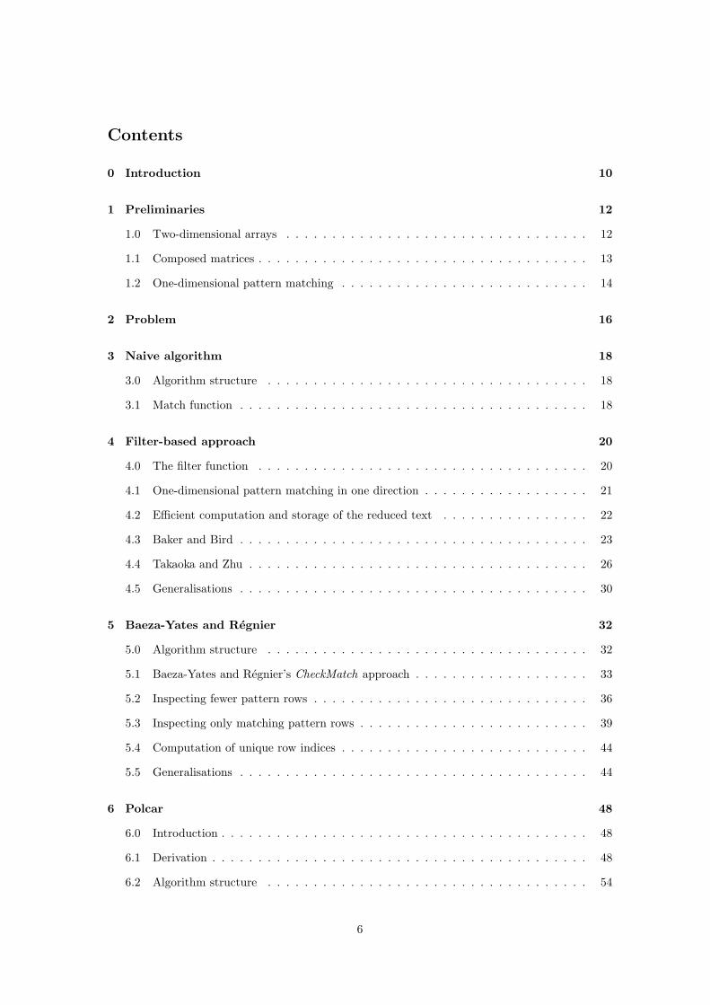
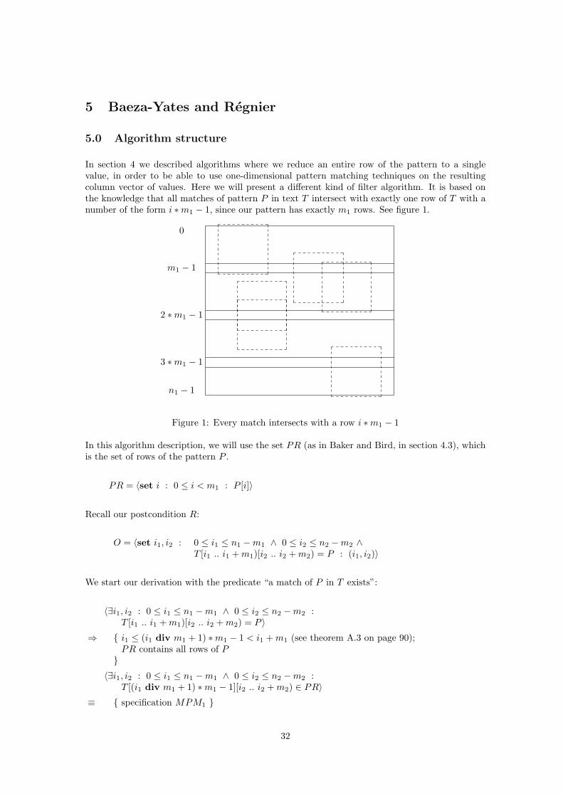
In section 4 we described algorithms where we reduce an entire row of the pattern to a singlevalue, in order to be able to use one-dimensional pattern matching techniques on the resultingcolumn vector of values. Here we will present a different kind of filter algorithm. It is based onthe knowledge that all matches of pattern P in text T intersect with exactly one row of T with anumber of the form i ∗m1 − 1, since our pattern has exactly m1 rows. See figure 1.

0

m1 − 1

2 ∗m1 − 1

3 ∗m1 − 1

n1 − 1

Figure 1: Every match intersects with a row i ∗m1 − 1

In this algorithm description, we will use the set PR (as in Baker and Bird, in section 4.3), whichis the set of rows of the pattern P .

PR = 〈set i : 0 ≤ i < m1 : P [i]〉

Recall our postcondition R:

O = 〈set i1, i2 : 0 ≤ i1 ≤ n1 −m1 ∧ 0 ≤ i2 ≤ n2 −m2 ∧T [i1 .. i1 + m1)[i2 .. i2 + m2) = P : (i1, i2)〉

We start our derivation with the predicate “a match of P in T exists”:

〈∃i1, i2 : 0 ≤ i1 ≤ n1 −m1 ∧ 0 ≤ i2 ≤ n2 −m2 :T [i1 .. i1 + m1)[i2 .. i2 + m2) = P 〉

⇒ { i1 ≤ (i1 div m1 + 1) ∗m1 − 1 < i1 + m1 (see theorem A.3 on page 90);PR contains all rows of P

}〈∃i1, i2 : 0 ≤ i1 ≤ n1 −m1 ∧ 0 ≤ i2 ≤ n2 −m2 :

T [(i1 div m1 + 1) ∗m1 − 1][i2 .. i2 + m2) ∈ PR〉≡ { specification MPM1 }

32

〈∃i1 : 0 ≤ i1 ≤ n1 −m1 : MPM1(PR, T [(i1 div m1 + 1) ∗m1 − 1]) 6= ?〉≡ { property ∃; dummy transformation: i = i1 div m1 + 1 }

〈∃i : 1 ≤ i ≤ n1 div m1 : MPM1(PR, T [i ∗m1 − 1]) 6= ?〉

For 0 ≤ k < m1, 1 ≤ i ≤ n1 div m1 and 0 ≤ j ≤ n2 −m2:

(j, P [k]) /∈ MPM1(PR, T [i ∗m1 − 1])

≡ { specification MPM1 }(j, P [k]) /∈ 〈set l, p, r : p ∈ PR ∧ T [i ∗m1 − 1] = lpr : (|l|, p)〉

≡ { set calculus, |P [k]| = m2, P [k] ∈ PR }T [i ∗m1 − 1][j .. j + m2) 6= P [k]

⇒ { • (i + 1) ∗m1 − 1− k ≤ n1 }T [i ∗m1 − 1− k .. (i + 1) ∗m1 − 1− k)[j .. j + m2) 6= P

If the above asumption, (i + 1) ∗m1 − 1− k ≤ n1, does not hold, then there can also be no matchstarting at row i ∗m1 − 1 − k, because it would not “fit” within the bounds of the text. So ouralgorithm will be of the following form:

for i : 1 ≤ i ≤ n1 div m1 →for j, p : (j, p) ∈ MPM1(PR, T [i ∗m1 − 1]) →

O := O ∪ 〈set k : 0 ≤ k < m1 ∧ (i + 1) ∗m1 − 1− k ≤ n1 ∧ P [k] = p ∧T [i ∗m1 − 1− k .. (i + 1) ∗m1 − 1− k)[j .. j + m2) = P :(i ∗m1 − 1− k, j)〉

rofrof

Note that the multipattern matching function MPM1 is always called with pattern set PR asits first parameter. Any precomputation, that depends on PR, necessary for the multipatternmatching algorithm needs to occur only once.

A simple implementation of this algorithm is the following:

for i : 1 ≤ i ≤ n1 div m1 →for j, p : (j, p) ∈ MPM1(PR, T [i ∗m1 − 1]) →

for k : 0 ≤ k < m1 ∧ (i + 1) ∗m1 − 1− k ≤ n1 →if P [k] = p →

if matchT,P (i ∗m1 − 1− k, j) → O := O ∪ {(i ∗m1 − 1− k, j)}[] ¬matchT,P (i ∗m1 − 1− k, j) → skipfi

[] P [k] 6= p → skipfi

rofrof

rof

5.1 Baeza-Yates and Regnier’s CheckMatch approach

While the algorithm we presented is correct, the call to matchT,P can lead to the same comparisonsbeing repeated several times. For instance, from our call to MPM1 and the guard P [k] = p we

33

can conclude that T [i ∗ m1 − 1][j .. j + m1) = P [k], yet each call to matchT,P will repeat thecomputation. Besides that, if more than one row of P is equal to string p, the matchT,P functionis called multiple times and there is some overlap in the rows of T that are being matched each time.This should be obvious if we look at the inner repition of the algorithm, with an implementationof matchT,P filled in.

for k : 0 ≤ k < m1 ∧ (i + 1) ∗m1 − 1− k ≤ n1 →if P [k] = p →

h, res := 0, true;do h 6= m1 ∧ res →

{ inv.: res ≡ T [i ∗m1 − 1− k .. i ∗m1 − 1− k + h)[j .. j + m2) = P [0 .. h) }res := T [i ∗m1 − 1− k + h][j .. j + m2) = P [h];h := h + 1

od;if res → O := O ∪ {(i ∗m1 − 1− k, j)}[] ¬res → skipfi

[] P [k] 6= p → skipfi

rof

This matchT,P implementation differs slightly from the one presented in section 3.1. Here weconsider entire rows in a fixed order, instead of single elements in an unspecified order. Wealso terminate the computation as soon as a mismatch is discovered, as suggested at the end ofsection 3.1.

To avoid the aforementioned unnecessary comparisons, we will keep a record of the rows of T thathave already been matched against the rows of P . To do this, we first introduce a unique indexfor each row of the pattern P . We introduce function g : Σ∗ → N:

{g(x) = 〈↓ l : 0 ≤ l < m1 ∧ x = P [l] : l〉 if x ∈ PRg(x) = m1 if x /∈ PR

(3)

For strings that occur as a row in the pattern P , the g-value is equal to the row number of theirfirst occurrence. This is a unique numbering for these strings; that is, for all x, y ∈ PR:

x = y ≡ g(x) = g(y)

In fact, we have the following property for g:

Theorem 5.0 For strings x and y, with g(y) 6= m1, we have:

x = y ≡ g(x) = g(y)

Proof Property x = y ⇒ g(x) = g(y) follows directly from the fact that g is a function. Weonly need to prove g(x) = g(y) ⇒ x = y, assuming g(y) 6= m1.

• Case: g(x) = m1.

34

(i− 1) ∗m1 − 1

i ∗m1 − 1

(i + 1) ∗m1 − 1

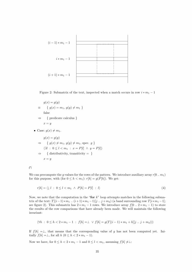
Figure 2: Submatrix of the text, inspected when a match occurs in row i ∗m1 − 1

g(x) = g(y)

≡ { g(x) = m1, g(y) 6= m1 }false

⇒ { predicate calculus }x = y

• Case: g(x) 6= m1.

g(x) = g(y)

⇒ { g(x) 6= m1, g(y) 6= m1, spec. g }〈∃l : 0 ≤ l < m1 : x = P [l] ∧ y = P [l]〉

⇒ { distributivity, transitivity = }x = y

�

We can precompute the g-values for the rows of the pattern. We introduce auxiliary array r[0 .. m1)for this purpose, with (for 0 ≤ h < m1): r[h] = g(P [h]). We get:

r[h] = 〈↓ l : 0 ≤ l < m1 ∧ P [h] = P [l] : l〉 (4)

Now, we note that the computation in the “for k” loop attempts matches in the following subma-trix of the text: T [(i−1)∗m1 .. (i+1)∗m1−1)[j .. j +m2) (a band surrounding row T [i∗m1−1];see figure 2). This submatrix has 2 ∗m1 − 1 rows. We introduce array f [0 .. 2 ∗m1 − 1) to storethe results of the row comparisons that have already been made. We will maintain the followinginvariant:

〈∀h : 0 ≤ h < 2 ∗m1 − 1 : f [h] =⊥ ∨ f [h] = g(T [(i− 1) ∗m1 + h][j .. j + m2))〉

If f [h] =⊥, that means that the corresponding value of g has not been computed yet. Ini-tially f [h] =⊥, for all h (0 ≤ h < 2 ∗m1 − 1).

Now we have, for 0 ≤ h < 2 ∗m1 − 1 and 0 ≤ l < m1, assuming f [h] 6=⊥:

35

T [(i− 1) ∗m1 + h][j .. j + m2) = P [l]

≡ { theorem 5.0 (page 34) }g(T [(i− 1) ∗m1 + h][j .. j + m2)) = g(P [l])

≡ { f [h] 6=⊥, invariant, spec. r }f [h] = r[l]

The algorithm now becomes:

for h : 0 ≤ h < 2 ∗m1 − 1 →f [h] :=⊥

rof ;{ T [i ∗m1 − 1][j .. j + m2) = p }f [m1 − 1] := g(p);for k : 0 ≤ k < m1 ∧ (i + 1) ∗m1 − 1− k ≤ n1 →

{ inv. 〈∀h : 0 ≤ h < 2 ∗m1 − 1 : f [h] =⊥ ∨ f [h] = g(T [(i− 1) ∗m1 + h][j .. j + m2))〉 }if r[k] = g(p) → { P [k] = p }

h, res := 0, true;do h 6= m1 ∧ res →

{ inv.: res ≡ T [i ∗m1 − 1− k .. i ∗m1 − 1− k + h)[j .. j + m2) = P [0 .. h) }if f [m1 − 1− k + h] =⊥ →

f [m1 − 1− k + h] := g(T [i ∗m1 − 1− k + h][j .. j + m2))[] f [m1 − 1− k + h] 6=⊥ → skipfi; { f [m1 − 1− k + h] 6=⊥ }res := f [m1 − 1− k + h] = r[h];h := h + 1

od;if res → O := O ∪ {(i ∗m1 − 1− k, j)}[] ¬res → skipfi

[] r[k] 6= g(p) → { P [k] 6= p } skipfi

rof

This is essentially the so-called Checkmatch function in Baeza-Yates and Regnier’s algorithm, aspresented in [BYR93]. The difference is that we have not specified how to compute the g-functionyet. We will get to that later, in section 5.4. Note that string variable p by itself is now no longerrelevant; we are only interested in its index, g(p).

We should note that we added f [m1 − 1] := g(p) to the intitialisation of f . We use the valueof g(p) in several other places in the algorithm (and f [m1 − 1] is likely to be inspected), so wemay as well initialise that value of f immediately.

5.2 Inspecting fewer pattern rows

In the version of the repetition presented in section 5.1, we examine for every value of k in therange [0 ↑ ((i + 1) ∗ m1 − 1 − n1), m1〉, whether row k of the pattern matches with string p. Ifso, we attempt to match the surrounding rows of the text with the corresponding rows of thepattern and conclude whether or not there is a match of our pattern in the text. However, aftersuch an attempted match, we may be able to use the last inspected value of f to conclude that

36

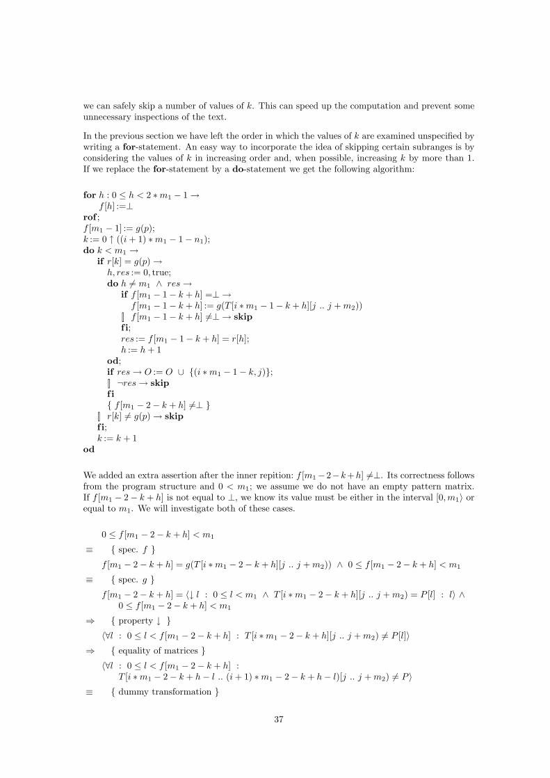
we can safely skip a number of values of k. This can speed up the computation and prevent someunnecessary inspections of the text.

In the previous section we have left the order in which the values of k are examined unspecified bywriting a for-statement. An easy way to incorporate the idea of skipping certain subranges is byconsidering the values of k in increasing order and, when possible, increasing k by more than 1.If we replace the for-statement by a do-statement we get the following algorithm:

for h : 0 ≤ h < 2 ∗m1 − 1 →f [h] :=⊥

rof ;f [m1 − 1] := g(p);k := 0 ↑ ((i + 1) ∗m1 − 1− n1);do k < m1 →

if r[k] = g(p) →h, res := 0, true;do h 6= m1 ∧ res →

if f [m1 − 1− k + h] =⊥ →f [m1 − 1− k + h] := g(T [i ∗m1 − 1− k + h][j .. j + m2))

[] f [m1 − 1− k + h] 6=⊥ → skipfi;res := f [m1 − 1− k + h] = r[h];h := h + 1

od;if res → O := O ∪ {(i ∗m1 − 1− k, j)};[] ¬res → skipfi{ f [m1 − 2− k + h] 6=⊥ }

[] r[k] 6= g(p) → skipfi;k := k + 1

od

We added an extra assertion after the inner repition: f [m1−2−k +h] 6=⊥. Its correctness followsfrom the program structure and 0 < m1; we assume we do not have an empty pattern matrix.If f [m1 − 2− k + h] is not equal to ⊥, we know its value must be either in the interval [0, m1〉 orequal to m1. We will investigate both of these cases.

0 ≤ f [m1 − 2− k + h] < m1

≡ { spec. f }f [m1 − 2− k + h] = g(T [i ∗m1 − 2− k + h][j .. j + m2)) ∧ 0 ≤ f [m1 − 2− k + h] < m1

≡ { spec. g }f [m1 − 2− k + h] = 〈↓ l : 0 ≤ l < m1 ∧ T [i ∗m1 − 2− k + h][j .. j + m2) = P [l] : l〉 ∧

0 ≤ f [m1 − 2− k + h] < m1

⇒ { property ↓ }〈∀l : 0 ≤ l < f [m1 − 2− k + h] : T [i ∗m1 − 2− k + h][j .. j + m2) 6= P [l]〉

⇒ { equality of matrices }〈∀l : 0 ≤ l < f [m1 − 2− k + h] :

T [i ∗m1 − 2− k + h− l .. (i + 1) ∗m1 − 2− k + h− l)[j .. j + m2) 6= P 〉≡ { dummy transformation }

37

〈∀l : i ∗m1 − 1− k + h− f [m1 − 2− k + h] ≤ l < i ∗m1 − 1− k + h :T [l .. l + m1)[j .. j + m2) 6= P 〉

So in this case, we can disregard the next (f [m1 − 2− k + h]− h + 1) ↑ 1 values of k.

f [m1 − 2− k + h] = m1

≡ { invariant }g(T [i ∗m1 − 2− k + h][j .. j + m2)) = m1

≡ { spec. g }T [i ∗m1 − 2− k + h][j .. j + m2) /∈ PR

⇒ { PR contains all rows of P }¬〈∃l : (i− 1) ∗m1 − 1− k + h ≤ l < i ∗m1 − 1− k + h : T [l .. l + m1)[j .. j + m2) = P 〉

So if we find an f -value of m1, we know we can skip the next m1 − h + 1 values of k. (We knowthat this is a positive number, since h ≤ m1.) We can rewrite this expression as follows:

m1 − h + 1

= { h ≤ m1 }(m1 − h + 1) ↑ 1

= { f [m1 − 2− k + h] = m1 }(f [m1 − 2− k + h]− h + 1) ↑ 1

This is the same expression we achieved in the case where f [m1−2−k+h] was in the interval [0, m1〉.The algorithm now becomes:

for h : 0 ≤ h < 2 ∗m1 − 1 →f [h] :=⊥

rof ;f [m1 − 1] := g(p);k := 0 ↑ ((i + 1) ∗m1 − 1− n1);do k < m1 →

if r[k] = g(p) →h, res := 0, true;do h 6= m1 ∧ res →

if f [m1 − 1− k + h] =⊥ →f [m1 − 1− k + h] := g(T [i ∗m1 − 1− k + h][j .. j + m2))

[] f [m1 − 1− k + h] 6=⊥ → skipfi;res := f [m1 − 1− k + h] = r[h];h := h + 1

od;if res → O := O ∪ {(i ∗m1 − 1− k, j)};[] ¬res → skipfi;k := k + (f [m1 − 2− k + h]− h + 1) ↑ 1

[] r[k] 6= g(p) → k := k + 1f i

od

38

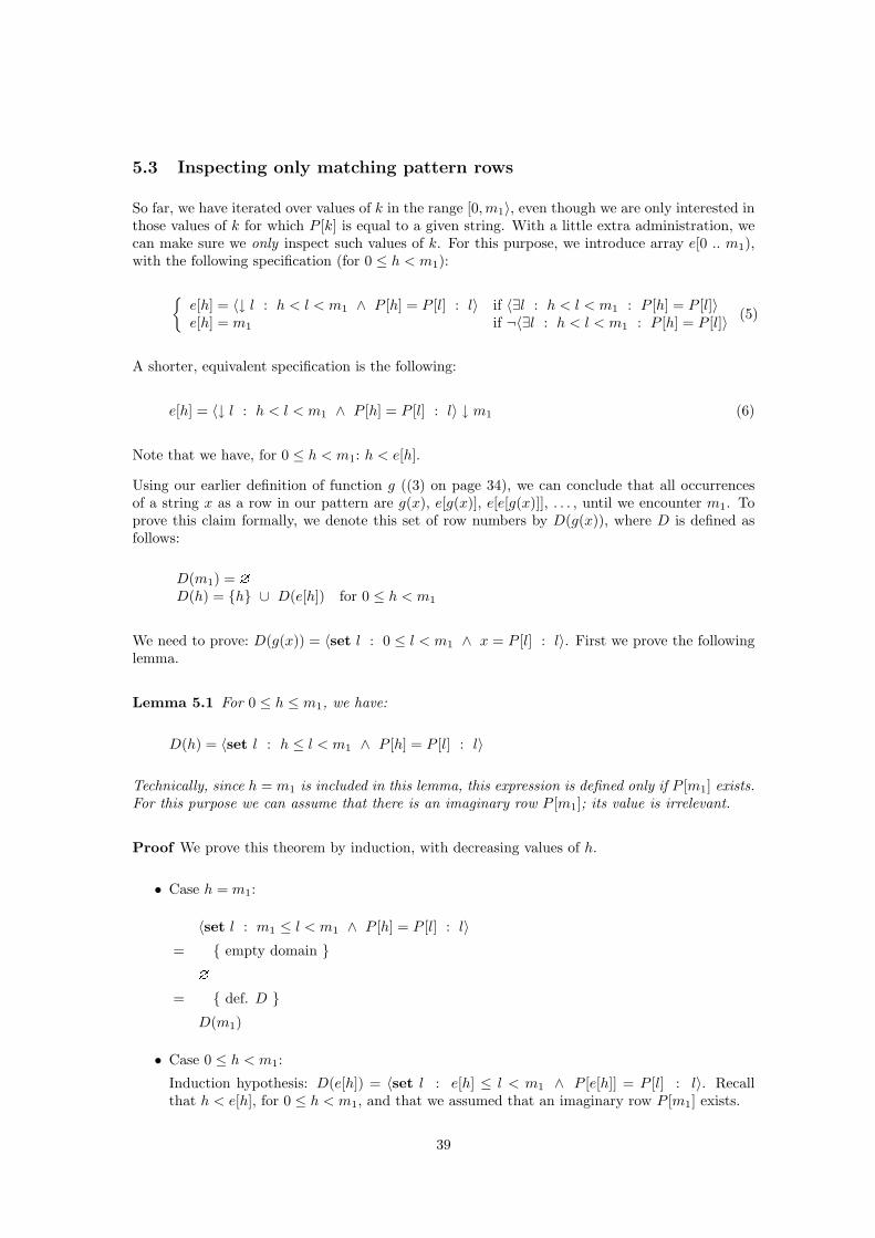
5.3 Inspecting only matching pattern rows

So far, we have iterated over values of k in the range [0, m1〉, even though we are only interested inthose values of k for which P [k] is equal to a given string. With a little extra administration, wecan make sure we only inspect such values of k. For this purpose, we introduce array e[0 .. m1),with the following specification (for 0 ≤ h < m1):

{e[h] = 〈↓ l : h < l < m1 ∧ P [h] = P [l] : l〉 if 〈∃l : h < l < m1 : P [h] = P [l]〉e[h] = m1 if ¬〈∃l : h < l < m1 : P [h] = P [l]〉 (5)

A shorter, equivalent specification is the following:

e[h] = 〈↓ l : h < l < m1 ∧ P [h] = P [l] : l〉 ↓ m1 (6)

Note that we have, for 0 ≤ h < m1: h < e[h].

Using our earlier definition of function g ((3) on page 34), we can conclude that all occurrencesof a string x as a row in our pattern are g(x), e[g(x)], e[e[g(x)]], . . . , until we encounter m1. Toprove this claim formally, we denote this set of row numbers by D(g(x)), where D is defined asfollows:

D(m1) = ?D(h) = {h} ∪ D(e[h]) for 0 ≤ h < m1

We need to prove: D(g(x)) = 〈set l : 0 ≤ l < m1 ∧ x = P [l] : l〉. First we prove the followinglemma.

Lemma 5.1 For 0 ≤ h ≤ m1, we have:

D(h) = 〈set l : h ≤ l < m1 ∧ P [h] = P [l] : l〉

Technically, since h = m1 is included in this lemma, this expression is defined only if P [m1] exists.For this purpose we can assume that there is an imaginary row P [m1]; its value is irrelevant.

Proof We prove this theorem by induction, with decreasing values of h.

• Case h = m1:

〈set l : m1 ≤ l < m1 ∧ P [h] = P [l] : l〉= { empty domain }

?

= { def. D }D(m1)

• Case 0 ≤ h < m1:

Induction hypothesis: D(e[h]) = 〈set l : e[h] ≤ l < m1 ∧ P [e[h]] = P [l] : l〉. Recallthat h < e[h], for 0 ≤ h < m1, and that we assumed that an imaginary row P [m1] exists.

39

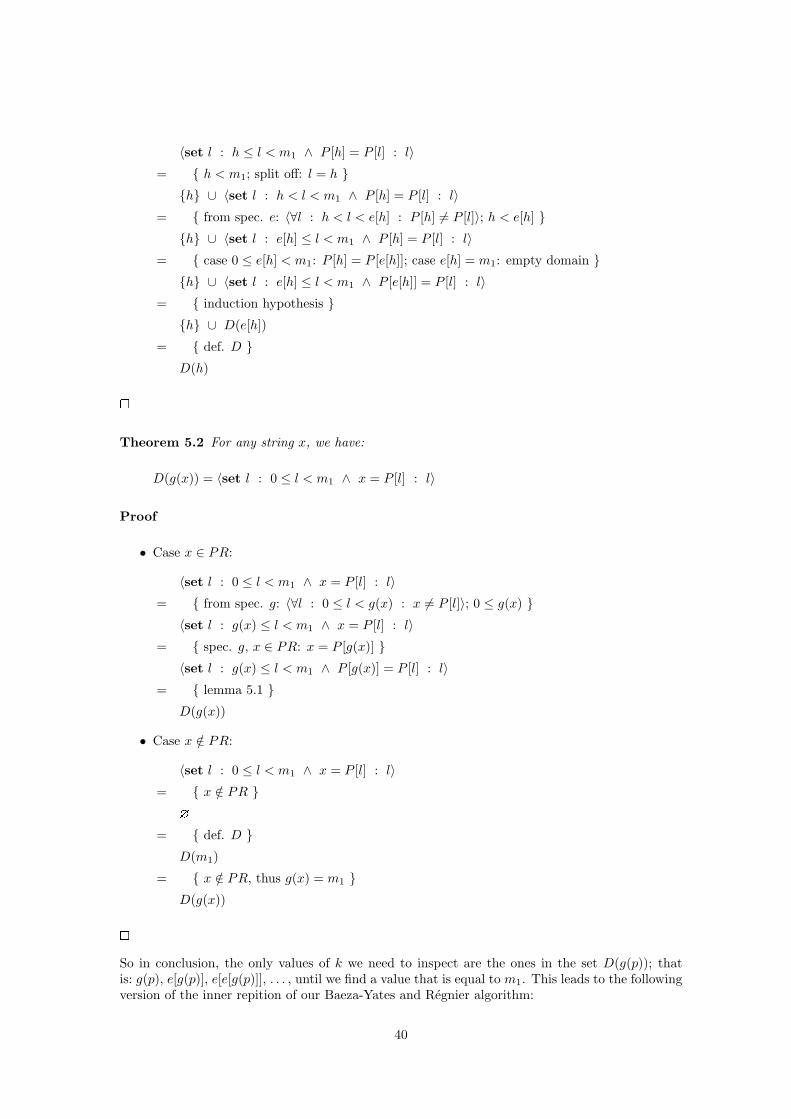
〈set l : h ≤ l < m1 ∧ P [h] = P [l] : l〉= { h < m1; split off: l = h }

{h} ∪ 〈set l : h < l < m1 ∧ P [h] = P [l] : l〉= { from spec. e: 〈∀l : h < l < e[h] : P [h] 6= P [l]〉; h < e[h] }

{h} ∪ 〈set l : e[h] ≤ l < m1 ∧ P [h] = P [l] : l〉= { case 0 ≤ e[h] < m1: P [h] = P [e[h]]; case e[h] = m1: empty domain }

{h} ∪ 〈set l : e[h] ≤ l < m1 ∧ P [e[h]] = P [l] : l〉= { induction hypothesis }

{h} ∪ D(e[h])

= { def. D }D(h)

�

Theorem 5.2 For any string x, we have:

D(g(x)) = 〈set l : 0 ≤ l < m1 ∧ x = P [l] : l〉

Proof

• Case x ∈ PR:

〈set l : 0 ≤ l < m1 ∧ x = P [l] : l〉= { from spec. g: 〈∀l : 0 ≤ l < g(x) : x 6= P [l]〉; 0 ≤ g(x) }

〈set l : g(x) ≤ l < m1 ∧ x = P [l] : l〉= { spec. g, x ∈ PR: x = P [g(x)] }

〈set l : g(x) ≤ l < m1 ∧ P [g(x)] = P [l] : l〉= { lemma 5.1 }

D(g(x))

• Case x /∈ PR:

〈set l : 0 ≤ l < m1 ∧ x = P [l] : l〉= { x /∈ PR }

?

= { def. D }D(m1)

= { x /∈ PR, thus g(x) = m1 }D(g(x))

�

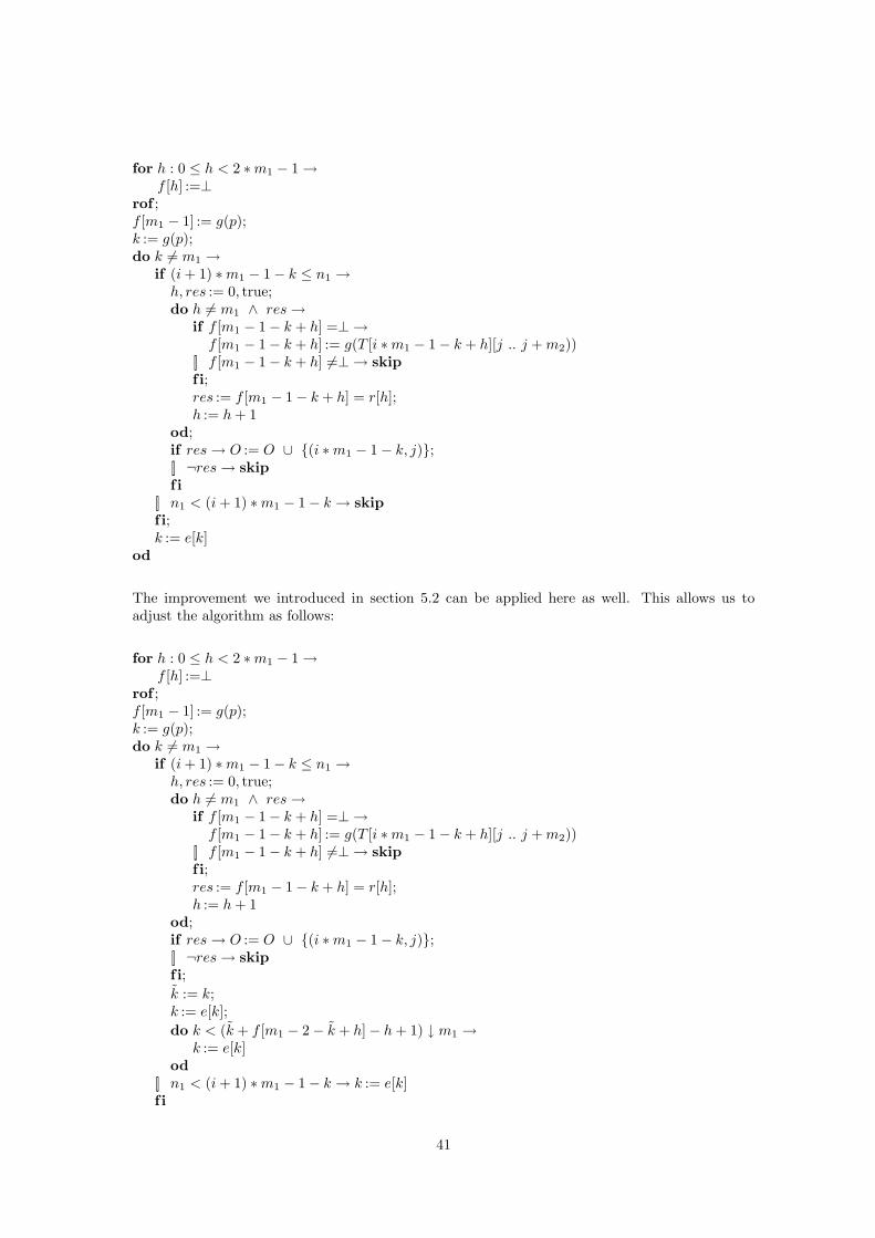
So in conclusion, the only values of k we need to inspect are the ones in the set D(g(p)); thatis: g(p), e[g(p)], e[e[g(p)]], . . . , until we find a value that is equal to m1. This leads to the followingversion of the inner repition of our Baeza-Yates and Regnier algorithm:

40

for h : 0 ≤ h < 2 ∗m1 − 1 →f [h] :=⊥

rof ;f [m1 − 1] := g(p);k := g(p);do k 6= m1 →

if (i + 1) ∗m1 − 1− k ≤ n1 →h, res := 0, true;do h 6= m1 ∧ res →

if f [m1 − 1− k + h] =⊥ →f [m1 − 1− k + h] := g(T [i ∗m1 − 1− k + h][j .. j + m2))

[] f [m1 − 1− k + h] 6=⊥ → skipfi;res := f [m1 − 1− k + h] = r[h];h := h + 1

od;if res → O := O ∪ {(i ∗m1 − 1− k, j)};[] ¬res → skipfi

[] n1 < (i + 1) ∗m1 − 1− k → skipfi;k := e[k]

od

The improvement we introduced in section 5.2 can be applied here as well. This allows us toadjust the algorithm as follows:

for h : 0 ≤ h < 2 ∗m1 − 1 →f [h] :=⊥

rof ;f [m1 − 1] := g(p);k := g(p);do k 6= m1 →

if (i + 1) ∗m1 − 1− k ≤ n1 →h, res := 0, true;do h 6= m1 ∧ res →

if f [m1 − 1− k + h] =⊥ →f [m1 − 1− k + h] := g(T [i ∗m1 − 1− k + h][j .. j + m2))

[] f [m1 − 1− k + h] 6=⊥ → skipfi;res := f [m1 − 1− k + h] = r[h];h := h + 1

od;if res → O := O ∪ {(i ∗m1 − 1− k, j)};[] ¬res → skipfi;k := k;k := e[k];do k < (k + f [m1 − 2− k + h]− h + 1) ↓ m1 →

k := e[k]od

[] n1 < (i + 1) ∗m1 − 1− k → k := e[k]f i

41

od

Computation of e

So far we have ignored the question how to initialise the values of array e. We can of course easilycome up with an implementation that, for each pattern row, searches for that row’s next occurencein the pattern using a bounded linear search. Using array r, this would give rise to an O(m1

2)algorithm. However, we can give an O(m1) algorithm.

Our postcondition is the specification of e, as given in (5) and, equivalently, (6) on page 39. Weintroduce integer variable i, along with the following invariants:

P0 : 0 ≤ i ≤ m1

P1 : 〈∀h : 0 ≤ h < m1 : e[h] = 〈↓ l : h < l < i ∧ P [h] = P [l] : l〉 ↓ m1〉

Then the postcondition is established when i = m1. Initially, we can choose i = 0 and e[h] = m1,for 0 ≤ h < m1. Ad P1(i := i + 1):

• For h: i ≤ h < m1:

〈↓ l : h < l < i + 1 ∧ P [h] = P [l] : l〉 ↓ m1

= { i ≤ h: empty domain }m1

= { i ≤ h: empty domain }〈↓ l : h < l < i ∧ P [h] = P [l] : l〉 ↓ m1

= { P1 }e[h]

• For h: 0 ≤ h < i:

〈↓ l : h < l < i + 1 ∧ P [h] = P [l] : l〉 ↓ m1

= { h < i; split off l = i }{〈↓ l : h < l < i ∧ P [h] = P [l] : l〉 ↓ m1 if P [h] 6= P [i]〈↓ l : h < l < i ∧ P [h] = P [l] : l〉 ↓ m1 ↓ i if P [h] = P [i]

= { P1 }{e[h] if P [h] 6= P [i]e[h] ↓ i if P [h] = P [i]

= { def. ↓, predicate calculus }{e[h] if P [h] 6= P [i] ∨ e[h] < ii if P [h] = P [i] ∧ i ≤ e[h]

= { P1: e[h] = m1 ∨ e[h] < i; i ≤ m1 }{e[h] if P [h] 6= P [i] ∨ e[h] 6= m1

i if P [h] = P [i] ∧ e[h] = m1

So the only values of h for which e[h] needs to be updated are the ones for which the followingholds: P [h] = P [i] ∧ e[h] = m1.

42

P [h] = P [i] ∧ e[h] = m1

≡ { P1 }P [h] = P [i] ∧ 〈↓ l : h < l < i ∧ P [h] = P [l] : l〉 ↓ m1 = m1

≡ { transitivity = }P [h] = P [i] ∧ 〈↓ l : h < l < i ∧ P [i] = P [l] : l〉 ↓ m1 = m1

≡ { i ≤ m1, definition ↓ }P [h] = P [i] ∧ 〈∀l : h < l < i : P [i] 6= P [l]〉

≡ { def. ↑, 0 ≤ h < i }h = 〈↑ l : 0 ≤ l < i ∧ P [i] = P [l] : l〉

≡ { g(P [i]) 6= m1, theorem 5.0 (see page 34) }h = 〈↑ l : 0 ≤ l < i ∧ g(P [i]) = g(P [l]) : l〉

≡ { spec. r }h = 〈↑ l : 0 ≤ l < i ∧ r[i] = r[l] : l〉

We conclude that there is at most one h for which e[h] needs to be updated, specifically: 〈↑ l :0 ≤ l < i ∧ r[i] = r[l] : l〉, if this value is greater than −∞. To find this value, we introduceauxiliary array aux[0 .. m1), with the following invariant.

P2 : 〈∀j : 0 ≤ j < m1 : aux[j] = 〈↑ l : 0 ≤ l < i ∧ j = r[l] : l〉〉

Initially, we have i = 0 and therefore aux[j] = −∞, for 0 ≤ j < m1. Ad P2(i := i + 1):

〈↑ l : 0 ≤ l < i + 1 ∧ j = r[l] : l〉= { split off: l = i }{

〈↑ l : 0 ≤ l < i ∧ j = r[l] : l〉 if j 6= r[i]〈↑ l : 0 ≤ l < i ∧ j = r[l] : l〉 ↑ i if j = r[i]

= { P2, math }{aux[j] if j 6= r[i]i if j = r[i]

In conclusion, this gives rise to the following initialisation algorithm for e:

for i : 0 ≤ i < m1 →e[i], aux[i] := m1,−∞

rof ;i := 0;do i 6= m1 →

if aux[r[i]] 6= −∞→e[aux[r[i]]] := i

[] aux[r[i]] = −∞→skip

fi;aux[r[i]] := i;i := i + 1

od

43

In an implementation we can represent −∞ by any negative number (or even any number outsideof the range [0, m1〉), for example: −1.

5.4 Computation of unique row indices

As we have seen in section 5.1, the value of string variable p is no longer of interest to us. Instead, weonly use g(p) (defined in (3) on page 34). For this reason, we want to introduce a new specificationfor one-dimensional multipattern matching, which returns the value of g(p) immediately.

MPM ′1(PS, t) = 〈set l, p, r : p ∈ PS ∧ t = lpr : (|l|, g(p))〉

The question remains, how to compute g-values. The method presented in [BYR93] is by buildingthe Aho-Corasick automaton based on set PR, with an output function λ that returns g-values.

More formally, our Aho-Corasick automaton of PR is a Moore machine (Q,Σ, ∆, δ, λ, q0). As insection 4.3, we will not go into every detail on how an Aho-Corasick automaton can be constructed;instead we refer to [WZ92], [WZ93] or [NR02].

Our output alphabet ∆ is equal to [0, m1]. For each state q, we want to establish: λ(q) = g(wq),where wq is the string consisting of the labels of the shortest path from start state q0 to q. Fornon-accepting states q we can simply define λ(q) = m1; for final states q, λ(q) needs to be equalto the index of the recognised row of P .

If we construct our Aho-Corasick automaton like a trie, by adding the rows of PR one by one, inincreasing order, we can establish this quite easily. Whenever we add a new final state q whileprocessing row l of our pattern matrix, we set λ(q) = l.

Now we have: g(p) = λ(δ∗(q0, p)). We can also use this Aho-Corasick automaton for our imple-mentation of MPM ′

1.

During the construction of the automaton we can also fill array r (as specified in (4) on page 35).After processing a row l of the pattern, the value of g(P [l]) is known and, by specification, this isthe required value of r[l].

5.5 Generalisations

The Baeza-Yates and Regnier algorithm can be generalised to be used for two-dimensional multi-pattern matching. Say we have l m1 ×m2 two-dimensional patterns: P0, P1, · · · , Pl−1. Then ourpostcondition becomes:

O = 〈set i1, i2, j : 0 ≤ i1 ≤ n1 −m1 ∧ 0 ≤ i2 ≤ n2 −m2 ∧ 0 ≤ j < l ∧T [i1 .. i1 + m1)[i2 .. i2 + m2) = Pj : (i1, i2, j)〉

We introduce a new auxiliary pattern matrix Q[0 .. l ∗m1)[0 .. m2), where (for 0 ≤ i < l ∗m1):

Q[i] = Pi div m1 [i mod m1]

Similarly to PR in the single-pattern searching algorithm, we introduce the set QR:

QR = 〈set i : 0 ≤ i < l ∗m1 : Q[i]〉

44

����

����

����

����

0 m1 − 1 2 ∗m1 − 1 3 ∗m1 − 1 n1

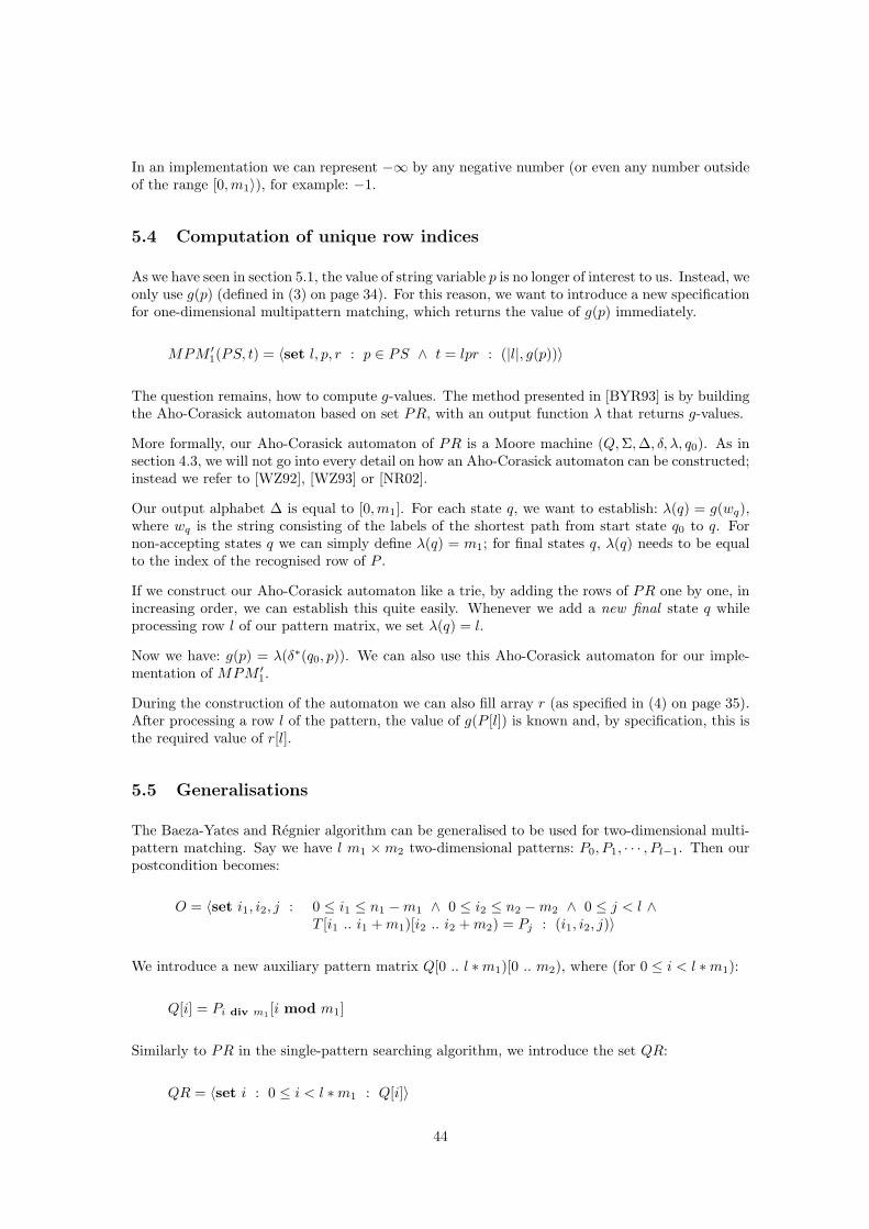
Figure 3: The Baeza-Yates algorithm idea, applied in three dimensions

Or, equivalently:

QR = 〈set i, j : 0 ≤ i < m1 ∧ 0 ≤ j < l : Pj [i]〉

Now we can apply one-dimensional multipattern matching to search for the strings in QR. Oncea match with one of these strings q ∈ QR has been found in one of the text’s rows, we need tocheck whether there is a match on that position in the text, with any of the pattern matrices inwhich q occurs as a row. That is, for each row Q[i] that is equal to q, we check if there is a matchwith pattern matrix Pi div m1 .

This boils down to only a slight modification of the Baeza-Yates and Regnier algorithm (or anyof the variations discussed). We will however need a slightly different definition for our g functionand auxialiary array r (and e, for the two algorithms presented in section 5.3). For any string xand 0 ≤ i < l ∗m1:{

g(x) = 〈↓ j : 0 ≤ j < l ∗m1 ∧ x = Q[j] : j〉 if x ∈ QRg(x) = l ∗m1 if x /∈ QR

r[i] = g(Q[i]){e[i] = 〈↓ j : i < j < l ∗m1 ∧ Q[i] = Q[j] : l〉 if 〈∃j : i < j < l ∗m1 : Q[i] = Q[j]〉e[i] = l ∗m1 if ¬〈∃j : i < j < l ∗m1 : Q[i] = Q[j]〉

The values of g, r and e can still be computed in the ways presented in sections 5.3 and 5.4.

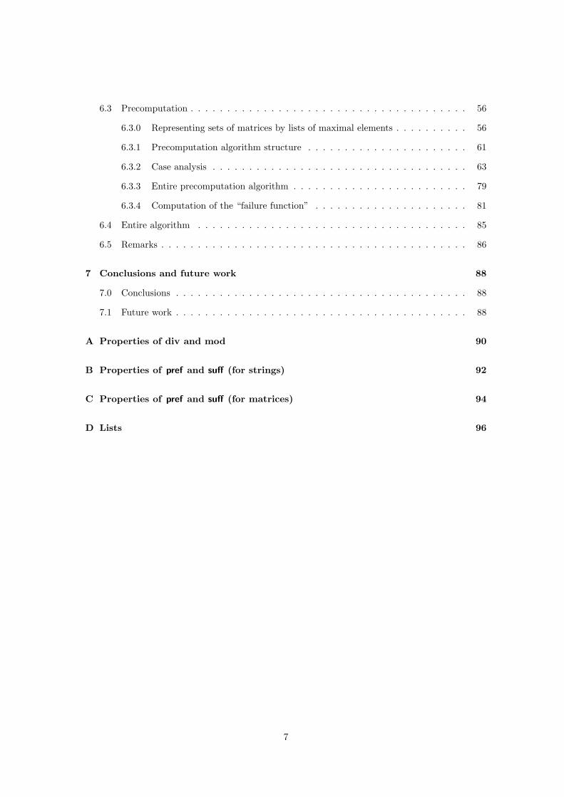
Matching in multiple dimensions is also possible using the Baeza-Yates and Regnier approach. Formatching in n + 1 dimensions (1 ≤ n) we use an n-dimensional multipattern matching algorithm.Here, too, we need to choose a different definition of g, namely a function that works on n-dimensional shapes. Also, if we are matching in more than two dimensions, we cannot simply usean Aho-Corasick automaton for multipattern matching and for computing our g-function.

For example, if we are matching in three dimensions, we regard the m1 × m2 × m3 pattern asa sequence of m1 two-dimensional matrices and the n1 × n2 × n3 text as a sequence of n1 two-

45

dimensional matrices. We then use two-dimensional multipattern matching to match every mth1

matrix of the text against the matrices of the pattern. (See also figure 3.) For every match foundwe check if there are any actual matches in three dimensions on that position.

46

47

6 Polcar

6.0 Introduction

In this section, we will present the algorithm that was presented by Tomas Polcar in [Pol04]; ashorter version of the same article can be found in [MP04].

The algorithm uses tessellation automata, a data structure introduced in [IN77]. In this presenta-tion however, we will attempt to derive the algorithm by manipulating sets of submatrices of thetext.

6.1 Derivation

P

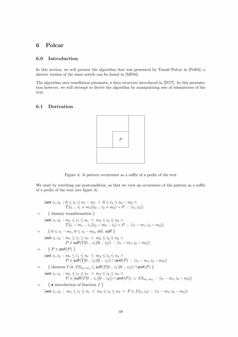
Figure 4: A pattern occurrence as a suffix of a prefix of the text

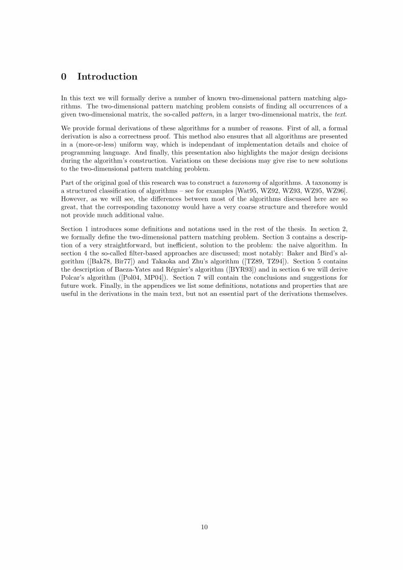
We start by rewriting our postcondition, so that we view an occurrence of the pattern as a suffixof a prefix of the text (see figure 4).

〈set i1, i2 : 0 ≤ i1 ≤ n1 −m1 ∧ 0 ≤ i2 ≤ n2 −m2 ∧T [i1 .. i1 + m1)[i2 .. i2 + m2) = P : (i1, i2)〉

= { dummy transformation }〈set i1, i2 : m1 ≤ i1 ≤ n1 ∧ m2 ≤ i2 ≤ n2 ∧

T [i1 −m1 .. i1)[i2 −m2 .. i2) = P : (i1 −m1, i2 −m2)〉= { 0 ≤ i1 −m1, 0 ≤ i2 −m2, def. suff }

〈set i1, i2 : m1 ≤ i1 ≤ n1 ∧ m2 ≤ i2 ≤ n2 ∧P ∈ suff(T [0 .. i1)[0 .. i2)) : (i1 −m1, i2 −m2)〉

= { P ∈ pref(P ) }〈set i1, i2 : m1 ≤ i1 ≤ n1 ∧ m2 ≤ i2 ≤ n2 ∧

P ∈ suff(T [0 .. i1)[0 .. i2)) ∩ pref(P ) : (i1 −m1, i2 −m2)〉= { theorem C.0: ESm1,m2 ⊆ suff(T [0 .. i1)[0 .. i2)) ∩ pref(P ) }

〈set i1, i2 : m1 ≤ i1 ≤ n1 ∧ m2 ≤ i2 ≤ n2 ∧P ∈ (suff(T [0 .. i1)[0 .. i2)) ∩ pref(P )) ∪ ESm1,m2 : (i1 −m1, i2 −m2)〉

= { • introduction of function f }〈set i1, i2 : m1 ≤ i1 ≤ n1 ∧ m2 ≤ i2 ≤ n2 ∧ P ∈ f(i1, i2) : (i1 −m1, i2 −m2)〉

48

We introduce function f : [0, n1]× [0, n2] → P(M2(Σ)), with the following specification:

f(i1, i2) = (suff(T [0 .. i1)[0 .. i2)) ∩ pref(P )) ∪ ESm1,m2

We have introduced this function because we can define f recursively and then (hopefully) con-struct an algorithm to compute f . Before we get to that, we introduce the following lemmas.

Lemma 6.0 concerns how the set of suffixes of a prefix of T can be split into a set of empty matricesand a set of nonempty matrices. Lemma 6.1 shows how we can conclude whether a submatrix ofthe text is a prefix of the pattern.

Lemma 6.0 For 0 ≤ i1 < n1 and 0 ≤ i2 < n2:

suff(T [0 .. i1 + 1)[0 .. i2 + 1)) =〈set j1, j2 : 0 ≤ j1 ≤ i1 ∧ 0 ≤ j2 ≤ i2 : T [j1 .. i1 + 1)[j2 .. i2 + 1)〉 ∪ ESi1+1,i2+1

Proof

suff(T [0 .. i1 + 1)[0 .. i2 + 1))

= { def. suff }〈set j1, j2 : 0 ≤ j1 ≤ i1 + 1 ∧ 0 ≤ j2 ≤ i2 + 1 : T [j1 .. i1 + 1)[j2 .. i2 + 1)〉

= { split off j1 = i1 + 1 and j2 = i2 + 1 }〈set j1, j2 : 0 ≤ j1 ≤ i1 ∧ 0 ≤ j2 ≤ i2 : T [j1 .. i1 + 1)[j2 .. i2 + 1)〉 ∪〈set j2 : 0 ≤ j2 ≤ i2 + 1 : E0,i2+1−j2〉 ∪ 〈set j1 : 0 ≤ j1 ≤ i1 + 1 : Ei1+1−j1,0〉

= { dummy transformation: j1 := i1 + 1− j }〈set j1, j2 : 0 ≤ j1 ≤ i1 ∧ 0 ≤ j2 ≤ i2 : T [j1 .. i1 + 1)[j2 .. i2 + 1)〉 ∪〈set j : 0 ≤ j ≤ i2 + 1 : E0,j〉 ∪ 〈set j : 0 ≤ j ≤ i1 + 1 : Ej,0〉

= { def. ES }〈set j1, j2 : 0 ≤ j1 ≤ i1 ∧ 0 ≤ j2 ≤ i2 : T [j1 .. i1 + 1)[j2 .. i2 + 1)〉 ∪ ESi1+1,i2+1

�

Lemma 6.1 For i1, j1, i2, j2 ∈ N, with j1 ≤ i1 < n1 and j2 ≤ i2 < n2:

• if i1 + 1− j1 ≤ m1 ∧ i2 + 1− j2 ≤ m2:

T [j1 .. i1 + 1)[j2 .. i2 + 1) ∈ pref(P ) ≡T [j1 .. i1)[j2 .. i2 + 1) ∈ pref(P ) ∧ T [j1 .. i1 + 1)[j2 .. i2) ∈ pref(P ) ∧T [i1, i2] = P [i1 − j1, i2 − j2]

• if m1 < i1 + 1− j1 ∨ m2 < i2 + 1− j2:

T [j1 .. i1 + 1)[j2 .. i2 + 1) /∈ pref(P )

Proof

• Case: i1 + 1− j1 ≤ m1 ∧ i2 + 1− j2 ≤ m2 (our submatrix is not larger than the pattern)

49

T [j1 .. i1 + 1)[j2 .. i2 + 1) ∈ pref(P )

≡ { def. pref }T [j1 .. i1 + 1)[j2 .. i2 + 1) ∈ 〈set l1, l2 : 0 ≤ l1 ≤ m1 ∧ 0 ≤ l2 ≤ m2 : P [0 .. l1)[0 .. l2)〉

≡ { i1 − j1 < m1, i2 − j2 < m2 }T [j1 .. i1 + 1)[j2 .. i2 + 1) = P [0 .. i1 + 1− j1)[0 .. i2 + 1− j2)

≡ { j1 ≤ i1, j2 ≤ i2, def. equality of matrices }T [j1 .. i1)[j2 .. i2 + 1) = P [0 .. i1 − j1)[0 .. i2 + 1− j2) ∧T [j1 .. i1 + 1)[j2 .. i2) = P [0 .. i1 + 1− j1)[0 .. i2 − j2) ∧T [i1, i2] = P [i1 − j1, i2 − j2]

≡ { i1 − j1 < m1, i2 − j2 < m2, def. pref }T [j1 .. i1)[j2 .. i2 + 1) ∈ pref(P ) ∧ T [j1 .. i1 + 1)[j2 .. i2) ∈ pref(P ) ∧T [i1, i2] = P [i1 − j1, i2 − j2]

• Case: m1 < i1 + 1− j1 ∨ m2 < i2 + 1− j2 (our submatrix is larger than the pattern)

T [j1 .. i1 + 1)[j2 .. i2 + 1) ∈ pref(P )

≡ { def. pref }T [j1 .. i1 + 1)[j2 .. i2 + 1) ∈ 〈set l1, l2 : 0 ≤ l1 ≤ m1 ∧ 0 ≤ l2 ≤ m2 : P [0 .. l1)[0 .. l2)〉

≡ { m1 ≤ i1 − j1 ∨ m2 ≤ i2 − j2 }false

�

Now we can get back to finding a recursive definition for f . For 0 ≤ i2 ≤ n2 we derive:

f(0, i2)

= { spec. f }(suff(T [0 .. 0)[0 .. i2)) ∩ pref(P )) ∪ ESm1,m2

= { def. submatrix }(suff(E0,i2) ∩ pref(P )) ∪ ESm1,m2

= { def. suff, one point rule, def. submatrix }(〈set j : 0 ≤ j ≤ i2 : E0,j〉 ∩ pref(P )) ∪ ESm1,m2

= { def. ES }(ES0,i2 ∩ pref(P )) ∪ ESm1,m2

= { theorem C.1 }ES0,i2↓m2 ∪ ESm1,m2

= { 0 ≤ m1, i2 ↓ m2 ≤ m2 }ESm1,m2

Symmetrically, we know that f(i1, 0) = ESm1,m2 (for 0 ≤ i1 ≤ n1). We will now examineexpression f(i1 + 1, i2 + 1), for 0 ≤ i1 < n1 and 0 ≤ i2 < n2.

f(i1 + 1, i2 + 1)

= { spec. f }

50

(suff(T [0 .. i1 + 1)[0 .. i2 + 1)) ∩ pref(P )) ∪ ESm1,m2

= { lemma 6.0 }((〈set j1, j2 : 0 ≤ j1 ≤ i1 ∧ 0 ≤ j2 ≤ i2 : T [j1 .. i1 + 1)[j2 .. i2 + 1)〉 ∪ ESi1+1,i2+1) ∩ pref(P )) ∪ESm1,m2

= { ∩ over ∪; theorem C.1 }(〈set j1, j2 : 0 ≤ j1 ≤ i1 ∧ 0 ≤ j2 ≤ i2 : T [j1 .. i1 + 1)[j2 .. i2 + 1)〉 ∩ pref(P )) ∪ES(i1+1)↓m1,(i2+1)↓m2 ∪ ESm1,m2

= { def. ES }(〈set j1, j2 : 0 ≤ j1 ≤ i1 ∧ 0 ≤ j2 ≤ i2 : T [j1 .. i1 + 1)[j2 .. i2 + 1)〉 ∩ pref(P )) ∪ ESm1,m2

= { property ∩ }〈set j1, j2 : 0 ≤ j1 ≤ i1 ∧ 0 ≤ j2 ≤ i2 ∧ T [j1 .. i1 + 1)[j2 .. i2 + 1) ∈ pref(P ) :

T [j1 .. i1 + 1)[j2 .. i2 + 1)〉 ∪ ESm1,m2

= { lemma 6.1 }〈set j1, j2 : 0 ≤ j1 ≤ i1 ∧ 0 ≤ j2 ≤ i2 ∧ i1 − j1 < m1 ∧ i2 − j2 < m2 ∧

T [j1 .. i1)[j2 .. i2 + 1) ∈ pref(P ) ∧ T [j1 .. i1 + 1)[j2 .. i2) ∈ pref(P ) ∧T [i1, i2] = P [i1 − j1, i2 − j2] : T [j1 .. i1 + 1)[j2 .. i2 + 1)〉 ∪ ESm1,m2

= { prop. matrices }〈set j1, j2 : 0 ≤ j1 ≤ i1 ∧ 0 ≤ j2 ≤ i2 ∧ i1 − j1 < m1 ∧ i2 − j2 < m2 ∧[

T [j1 .. i1)[j2 .. i2) T [j1 .. i1)[i2]]∈ pref(P ) ∧[

T [j1 .. i1)[j2 .. i2)T [i1][j2 .. i2)

]∈ pref(P ) ∧

T [i1, i2] = P [i1 − j1, i2 − j2] :[

T [j1 .. i1)[j2 .. i2) T [j1 .. i1)[i2]T [i1][j2 .. i2) T [i1, i2]

]〉 ∪ ESm1,m2

= { one-point rule }〈set j1, j2, A, b, c : 0 ≤ j1 ≤ i1 ∧ 0 ≤ j2 ≤ i2 ∧ i1 − j1 < m1 ∧ i2 − j2 < m2 ∧

A = T [j1 .. i1)[j2 .. i2) ∧ b = T [j1 .. i1)[i2] ∧ c = T [i1][j2 .. i2) ∧[A b

]∈ pref(P ) ∧

[Ac

]∈ pref(P ) ∧ T [i1, i2] = P [i1 − j1, i2 − j2] :[

A bc T [i1, i2]

]〉 ∪ ESm1,m2

= { prop. matrices }〈set j1, j2, A, b, c : 0 ≤ j1 ≤ i1 ∧ 0 ≤ j2 ≤ i2 ∧ i1 − j1 < m1 ∧ i2 − j2 < m2 ∧[

A b]

= T [j1 .. i1)[j2 .. i2 + 1) ∧ row(b) = row(A) ∧ col(b) = 1 ∧[Ac

]= T [j1 .. i1 + 1)[j2 .. i2) ∧ row(c) = 1 ∧ col(c) = col(A) ∧[

A b]∈ pref(P ) ∧

[Ac

]∈ pref(P ) ∧ T [i1, i2] = P [i1 − j1, i2 − j2] :[

A bc T [i1, i2]

]〉 ∪ ESm1,m2

= { one-point rule: j1 = i1 − row(A), j2 = i2 − col(A); def. suff }〈set A, b, c : row(A) < m1 ∧ col(A) < m2 ∧

row(b) = row(A) ∧ col(b) = 1 ∧ row(c) = 1 ∧ col(c) = col(A) ∧[A b

]∈ suff(T [0 .. i1)[0 .. i2 + 1)) ∧

[Ac

]∈ suff(T [0 .. i1 + 1)[0 .. i2)) ∧[

A b]∈ pref(P ) ∧

[Ac

]∈ pref(P ) ∧ T [i1, i2] = P [row(A), col(A)] :

51

[A bc T [i1, i2]

]〉 ∪ ESm1,m2

= { set calculus }〈set A, b, c : row(A) < m1 ∧ col(A) < m2 ∧

row(b) = row(A) ∧ col(b) = 1 ∧ row(c) = 1 ∧ col(c) = col(A) ∧[A b

]∈ suff(T [0 .. i1)[0 .. i2 + 1)) ∩ pref(P ) ∧[

Ac

]∈ suff(T [0 .. i1 + 1)[0 .. i2)) ∩ pref(P ) ∧ T [i1, i2] = P [row(A), col(A)] :[

A bc T [i1, i2]

]〉 ∪ ESm1,m2

= { • (?) }〈set A, b, c : row(A) < m1 ∧ col(A) < m2 ∧

row(b) = row(A) ∧ col(b) = 1 ∧ row(c) = 1 ∧ col(c) = col(A) ∧[A b

]∈ (suff(T [0 .. i1)[0 .. i2 + 1)) ∩ pref(P )) ∪ ESm1,m2 ∧[

Ac

]∈ (suff(T [0 .. i1 + 1)[0 .. i2)) ∩ pref(P )) ∪ ESm1,m2 ∧ T [i1, i2] = P [row(A), col(A)] :[

A bc T [i1, i2]

]〉 ∪ ESm1,m2

= { def. f }〈set A, b, c : row(A) < m1 ∧ col(A) < m2 ∧

row(b) = row(A) ∧ col(b) = 1 ∧ row(c) = 1 ∧ col(c) = col(A) ∧[A b

]∈ f(i1, i2 + 1) ∧

[Ac

]∈ f(i1 + 1, i2) ∧ T [i1, i2] = P [row(A), col(A)] :[

A bc T [i1, i2]

]〉 ∪ ESm1,m2

= { • introduction of δ }δ(f(i1, i2 + 1), f(i1 + 1, i2), T [i1, i2])

Ad (?): we still need to justify that we can introduce ESm1,m2 in this step of the derivation. Weassume we have A, b and c, satisfying:

row(A) < m1 ∧ col(A) < m2 ∧row(b) = row(A) ∧ col(b) = 1 ∧ row(c) = 1 ∧ col(c) = col(A) ∧[

A b]∈ (suff(T [0 .. i1)[0 .. i2 + 1)) ∩ pref(P )) ∪ ESm1,m2 ∧[

Ac

]∈ (suff(T [0 .. i1 + 1)[0 .. i2)) ∩ pref(P )) ∪ ESm1,m2

We derive:

[A b

]∈ ESm1,m2

≡ { definition ES }[A b

]∈ 〈set j : 0 ≤ j ≤ m1 : Ej,0〉 ∪ 〈set j : 0 ≤ j ≤ m2 : E0,j〉

≡ { col(b) = 1, therefore 0 < col([

A b]) }[

A b]∈ 〈set j : 0 ≤ j ≤ m2 : E0,j〉

⇒ { set calculus, definition E }row(

[A b

]) = 0 ∧ 0 < col(

[A b

]) ≤ m2

≡ { def. row, col; col(b) = 1 }

52

row(A) = 0 ∧ 0 ≤ col(A) < m2

≡ { def. row, col; row(c) = 1 }

row([

Ac

]) = 1 ∧ 0 ≤ col(

[Ac

]) < m2

≡ {[

Ac

]∈ (suff(T [0 .. i1 + 1)[0 .. i2)) ∩ pref(P )) ∪ ESm1,m2 ;

row([

Ac

]) = 1 ∧

[Ac

]∈ ESm1,m2 ⇒ col(

[Ac

]) = 0

}

row([

Ac

]) = 1 ∧ 0 ≤ col(

[Ac

]) < i2 + 1 ↓ m2

≡ { def. row, col; row(c) = 1 }row(A) = 0 ∧ 0 ≤ col(A) < i2 + 1 ↓ m2

≡ { def. row, col; col(b) = 1 }row(

[A b

]) = 0 ∧ 0 < col(

[A b

]) ≤ i2 + 1 ↓ m2

≡ { definition ES }[A b

]∈ ES0,i2+1↓m2

⇒ { theorem C.0 }[A b

]∈ suff(T [0 .. i1)[0 .. i2 + 1)) ∩ pref(P )

Symmetrically,[

Ac

]∈ ESm1,m2 ⇒

[Ac

]∈ suff(T [0 .. i1 + 1)[0 .. i2)) ∩ pref(P ). The step

marked (?) is therefore correct.

We introduce function δ : P(pref(P ))× P(pref(P ))× Σ → P(pref(P )), with the following specifi-cation:

δ(Q, R, σ) = 〈set A, b, c : SIZE (A, b, c) ∧[

A b]∈ Q ∧

[Ac

]∈ R ∧

σ = P [row(A), col(A)] :[

A bc σ

]〉 ∪ ESm1,m2

Here we have used the auxiliary predicate SIZE : M2(Σ)×M2(Σ)×M2(Σ) → B, which is definedas follows:

SIZE (A, b, c) ≡ row(A) < m1 ∧ col(A) < m2 ∧row(b) = row(A) ∧ col(b) = 1 ∧ row(c) = 1 ∧ col(c) = col(A)

The expression SIZE (A, b, c) means that matrices A, b and c have such sizes that, for any additional

symbol σ, the matrix[

A bc σ

]is well-defined and not larger, in either dimension, than the

pattern P .

53

6.2 Algorithm structure

In summary of what we have seen so far, we have specified function f and derived the correctnessof the following way to compute f :

f(0, i2) = ESm1,m2 (0 ≤ i2 ≤ n2)f(i1, 0) = ESm1,m2 (0 ≤ i1 ≤ n1)

f(i1 + 1, i2 + 1) = δ(f(i1, i2 + 1), f(i1 + 1, i2), T [i1, i2]) (0 ≤ i1 < n1, 0 ≤ i2 < n2)

We are interested in those values of i1 and i2, with m1 ≤ i1 ≤ n1 and m2 ≤ i2 ≤ n2, where thefollowing holds: P ∈ f(i1, i2). A solution to the two-dimensional pattern matching problem is tocompute all values of f(i1, i2) (for 0 ≤ i1 ≤ n1, 0 ≤ i2 ≤ n2) and then do a membership test onthe relevant values. This gives rise to the following algorithm:

O := ?;for i1 : 0 ≤ i1 ≤ n1 → f(i1, 0) := ESm1,m2 rof ;for i2 : 0 ≤ i2 ≤ n2 → f(0, i2) := ESm1,m2 rof ;i1 := 0;do i1 6= n1 →

i2 := 0;do i2 6= n2 →

f(i1 + 1, i2 + 1) := δ(f(i1, i2 + 1), f(i1 + 1, i2), T [i1, i2]);i2 := i2 + 1

od;i1 := i1 + 1

od;for i1, i2 : m1 ≤ i1 ≤ n1 ∧ m2 ≤ i2 ≤ n2 →

if P ∈ f(i1, i2) → O := O ∪ {(i1 −m1, i2 −m2)}[] P /∈ f(i1, i2) → skipfi

rof

However, if we assume that the pattern is not an empty matrix2, we can report the matches whilecomputing f . To show this we will further rewrite the postcondition. First we introduce a lemma,stating that there can be no occurrence of P in a prefix of T that is too small in either dimension.

Lemma 6.2 For 0 ≤ i1 < m1 and 0 ≤ i2 < m2:

P /∈ f(i1, i2)

Proof

P ∈ f(i1, i2)

≡ { definition f }P ∈ (suff(T [0 .. i1)[0 .. i2)) ∩ pref(P )) ∪ ESm1,m2

≡ { P /∈ ES }2If P is an empty matrix, the two-dimensional pattern matching problem is fairly trivial in itself, so (as in

previous algorithms) we can safely assume that P /∈ ES; we will not consider the case of an empty pattern in theremainder of this section.

54

P ∈ suff(T [0 .. i1)[0 .. i2)) ∩ pref(P )

≡ { P ∈ pref(P ) }P ∈ suff(T [0 .. i1)[0 .. i2))

≡ { i1 < m1 ∨ i2 < m2 }false

�

Now we can derive:

〈set i1, i2 : m1 ≤ i1 ≤ n1 ∧ m2 ≤ i2 ≤ n2 ∧ P ∈ f(i1, i2) : (i1 −m1, i2 −m2)〉= { P /∈ ES, therefore: 1 ≤ m1 and 1 ≤ m2; lemma 6.2 }

〈set i1, i2 : 1 ≤ i1 ≤ n1 ∧ 1 ≤ i2 ≤ n2 ∧ P ∈ f(i1, i2) : (i1 −m1, i2 −m2)〉

This gives rise to the following algorithm:

O := ?;for i1 : 0 ≤ i1 ≤ n1 → f(i1, 0) := ESm1,m2 rof ;for i2 : 0 ≤ i2 ≤ n2 → f(0, i2) := ESm1,m2 rof ;i1 := 0;do i1 6= n1 →

i2 := 0;do i2 6= n2 →

f(i1 + 1, i2 + 1) := δ(f(i1, i2 + 1), f(i1 + 1, i2), T [i1, i2]);if P ∈ f(i1 + 1, i2 + 1) → O := O ∪ {(i1 + 1−m1, i2 + 1−m2)}[] P /∈ f(i1 + 1, i2 + 1) → skipfi;i2 := i2 + 1

od;i1 := i1 + 1

od

Here we can introduce a space improvement, similarly to what we have done for the filter-basedalgorithms in section 4.2. Instead of storing all (n1+1)∗(n2+1) values of f , an array of length n2+1suffices. Let us call this array e and introduce the following invariant:

〈∀j : 0 ≤ j ≤ i2 : e[j] = f(i1 + 1, j)〉 ∧ 〈∀j : i2 < j ≤ n2 : e[j] = f(i1, j)〉

This gives us the following algorithm:

O := ?;for j : 0 ≤ j ≤ n2 → e[j] := ESm1,m2 rof ;i1, i2 := 0, 0;do i1 6= n1 →

do i2 6= n2 →e[i2 + 1] := δ(e[i2 + 1], e[i2], T [i1, i2]);if P ∈ e[i2 + 1] → O := O ∪ {(i1 + 1−m1, i2 + 1−m2)}[] P /∈ e[i2 + 1] → skip

55

f i;i2 := i2 + 1

od;i2 := 0;i1 := i1 + 1

od

6.3 Precomputation

6.3.0 Representing sets of matrices by lists of maximal elements

The algorithm given in section 6.2 is correct, if we can find a way to compute δ. However,computation of δ(Q, R, σ) can be rather inefficient, so repeating this for each element of the,potentially very large, text is undesirable. We would prefer precomputing the values of δ. We donot need to precompute δ(Q, R, σ) for all Q,R ⊆ pref(P ), since not all such sets Q and R canactually occur. We only need to examine reachable sets of prefixes of P .

Definition 6.3 (Reachability) The set of all reachable sets of prefixes of P is the smallest set Vsatisfying:

• ESm1,m2 ∈ V ;

• if Q,R ∈ V and σ ∈ Σ then δ(Q,R, σ) ∈ V .

We will now prove two properties of reachable sets of prefixes of P .

Theorem 6.4 Let S be a reachable set of prefixes of P . Then we have:

〈∀A,B : A ∈ S ∧ B ∈ suff(A) ∩ pref(P ) : B ∈ S〉

Proof We prove this by structural induction.

• S = ESm1,m2 .

A ∈ ESm1,m2 ∧ B ∈ suff(A) ∩ pref(P )

⇒ { def. ES, def. suff }((row(A) = 0 ∧ col(A) ≤ m2) ∨ (row(A) ≤ m1 ∧ col(A) = 0)) ∧

row(B) ≤ row(A) ∧ col(B) ≤ col(A)

⇒ { pred. calc, math }(row(B) = 0 ∧ col(B) ≤ m2) ∨ (row(B) ≤ m1 ∧ col(B) = 0)

≡ { def. ES }B ∈ ESm1,m2

• S = δ(Q, R, σ), for some reachable Q,R ⊆ pref(P ) and σ ∈ Σ. Our induction hypothesis is:

〈∀A, B : A ∈ Q ∧ B ∈ suff(A) ∩ pref(P ) : B ∈ Q〉 ∧〈∀A, B : A ∈ R ∧ B ∈ suff(A) ∩ pref(P ) : B ∈ R〉

56

We must prove:

〈∀A, B : A ∈ δ(Q,R, σ) ∧ B ∈ suff(A) ∩ pref(P ) : B ∈ δ(Q, R, σ)〉

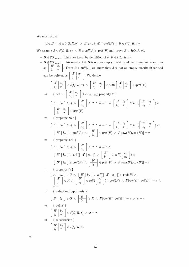
We assume A ∈ δ(Q,R, σ) ∧ B ∈ suff(A) ∩ pref(P ) and prove B ∈ δ(Q, R, σ).

– B ∈ ESm1,m2 . Then we have, by definition of δ: B ∈ δ(Q, R, σ).

– B /∈ ESm1,m2 . This means that B is not an empty matrix and can therefore be written

as[

B′ b0

b1 τ

]. From B ∈ suff(A) we know that A is not an empty matrix either and

can be written as[

A′ a0

a1 τ

]. We derive:[

A′ a0

a1 τ

]∈ δ(Q,R, σ) ∧

[B′ b0

b1 τ

]∈ suff(

[A′ a0

a1 τ

]) ∩ pref(P )

⇒ { def. δ,[

A′ a0

a1 τ

]/∈ ESm1,m2 ; property ∩ }

[A′ a0

]∈ Q ∧

[A′

a1

]∈ R ∧ σ = τ ∧

[B′ b0

b1 τ

]∈ suff(

[A′ a0

a1 τ

]) ∧[

B′ b0

b1 τ

]∈ pref(P )

≡ { property pref }[A′ a0

]∈ Q ∧

[A′

a1

]∈ R ∧ σ = τ ∧

[B′ b0

b1 τ

]∈ suff(

[A′ a0

a1 τ

]) ∧[

B′ b0

]∈ pref(P ) ∧

[B′

b1

]∈ pref(P ) ∧ P [row(B′), col(B′)] = τ

≡ { property suff }[A′ a0

]∈ Q ∧

[A′

a1

]∈ R ∧ σ = τ ∧[

B′ b0

]∈ suff(

[A′ a0

]) ∧

[B′

b1

]∈ suff(

[A′

a1

]) ∧[

B′ b0

]∈ pref(P ) ∧

[B′

b1

]∈ pref(P ) ∧ P [row(B′), col(B′)] = τ

≡ { property ∩ }[A′ a0

]∈ Q ∧

[B′ b0

]∈ suff(

[A′ a0

]) ∩ pref(P ) ∧[

A′

a1

]∈ R ∧

[B′

b1

]∈ suff(

[A′

a1

]) ∩ pref(P ) ∧ P [row(B′), col(B′)] = τ ∧

σ = τ

⇒ { induction hypothesis }[B′ b0

]∈ Q ∧

[B′

b1

]∈ R ∧ P [row(B′), col(B′)] = τ ∧ σ = τ

⇒ { def. δ }[B′ b0

b1 τ

]∈ δ(Q, R, τ) ∧ σ = τ

⇒ { substitution }[B′ b0

b1 τ

]∈ δ(Q, R, σ)

�

57

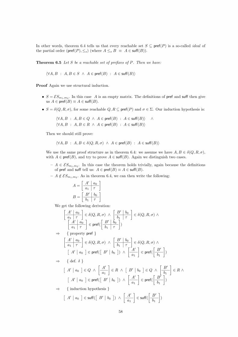
In other words, theorem 6.4 tells us that every reachable set S ⊆ pref(P ) is a so-called ideal ofthe partial order (pref(P ),≤s) (where A ≤s B ≡ A ∈ suff(B)).

Theorem 6.5 Let S be a reachable set of prefixes of P . Then we have:

〈∀A,B : A,B ∈ S ∧ A ∈ pref(B) : A ∈ suff(B)〉

Proof Again we use structural induction.

• S = ESm1,m2 . In this case A is an empty matrix. The definitions of pref and suff then giveus A ∈ pref(B) ≡ A ∈ suff(B).

• S = δ(Q, R, σ), for some reachable Q,R ⊆ pref(P ) and σ ∈ Σ. Our induction hypothesis is:

〈∀A, B : A, B ∈ Q ∧ A ∈ pref(B) : A ∈ suff(B)〉 ∧〈∀A,B : A,B ∈ R ∧ A ∈ pref(B) : A ∈ suff(B)〉

Then we should still prove:

〈∀A, B : A, B ∈ δ(Q, R, σ) ∧ A ∈ pref(B) : A ∈ suff(B)〉

We use the same proof structure as in theorem 6.4: we assume we have A, B ∈ δ(Q, R, σ),with A ∈ pref(B), and try to prove A ∈ suff(B). Again we distinguish two cases.

– A ∈ ESm1,m2 . In this case the theorem holds trivially, again because the definitionsof pref and suff tell us: A ∈ pref(B) ≡ A ∈ suff(B).

– A /∈ ESm1,m2 . As in theorem 6.4, we can then write the following:

A =[

A′ a0

a1 τ

]B =

[B′ b0

b1 τ

]We get the following derivation:[

A′ a0

a1 τ

]∈ δ(Q,R, σ) ∧

[B′ b0

b1 τ

]∈ δ(Q, R, σ) ∧[

A′ a0

a1 τ

]∈ pref(

[B′ b0

b1 τ

])

⇒ { property pref }[A′ a0

a1 τ

]∈ δ(Q,R, σ) ∧

[B′ b0

b1 τ

]∈ δ(Q, R, σ) ∧[

A′ a0

]∈ pref(

[B′ b0

]) ∧

[A′

a1

]∈ pref(

[B′

b1

])

⇒ { def. δ }[A′ a0

]∈ Q ∧

[A′

a1

]∈ R ∧

[B′ b0

]∈ Q ∧

[B′

b1

]∈ R ∧[

A′ a0

]∈ pref(

[B′ b0

]) ∧

[A′

a1

]∈ pref(

[B′

b1

])

⇒ { induction hypothesis }[A′ a0

]∈ suff(

[B′ b0

]) ∧

[A′

a1

]∈ suff(

[B′

b1

])

58

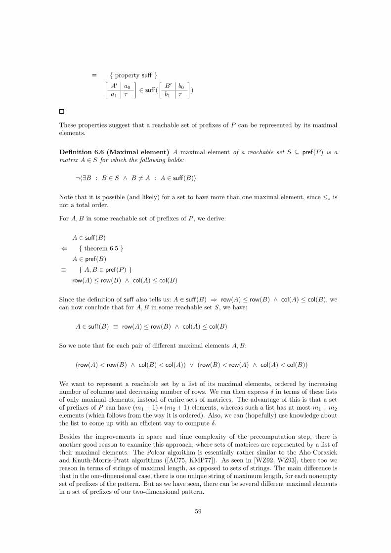
≡ { property suff }[A′ a0

a1 τ

]∈ suff(

[B′ b0

b1 τ

])

�

These properties suggest that a reachable set of prefixes of P can be represented by its maximalelements.

Definition 6.6 (Maximal element) A maximal element of a reachable set S ⊆ pref(P ) is amatrix A ∈ S for which the following holds:

¬〈∃B : B ∈ S ∧ B 6= A : A ∈ suff(B)〉

Note that it is possible (and likely) for a set to have more than one maximal element, since ≤s isnot a total order.

For A,B in some reachable set of prefixes of P , we derive:

A ∈ suff(B)

⇐ { theorem 6.5 }A ∈ pref(B)

≡ { A, B ∈ pref(P ) }row(A) ≤ row(B) ∧ col(A) ≤ col(B)

Since the definition of suff also tells us: A ∈ suff(B) ⇒ row(A) ≤ row(B) ∧ col(A) ≤ col(B), wecan now conclude that for A, B in some reachable set S, we have:

A ∈ suff(B) ≡ row(A) ≤ row(B) ∧ col(A) ≤ col(B)

So we note that for each pair of different maximal elements A, B:

(row(A) < row(B) ∧ col(B) < col(A)) ∨ (row(B) < row(A) ∧ col(A) < col(B))

We want to represent a reachable set by a list of its maximal elements, ordered by increasingnumber of columns and decreasing number of rows. We can then express δ in terms of these listsof only maximal elements, instead of entire sets of matrices. The advantage of this is that a setof prefixes of P can have (m1 + 1) ∗ (m2 + 1) elements, whereas such a list has at most m1 ↓ m2

elements (which follows from the way it is ordered). Also, we can (hopefully) use knowledge aboutthe list to come up with an efficient way to compute δ.

Besides the improvements in space and time complexity of the precomputation step, there isanother good reason to examine this approach, where sets of matrices are represented by a list oftheir maximal elements. The Polcar algorithm is essentially rather similar to the Aho-Corasickand Knuth-Morris-Pratt algorithms ([AC75, KMP77]). As seen in [WZ92, WZ93], there too wereason in terms of strings of maximal length, as opposed to sets of strings. The main difference isthat in the one-dimensional case, there is one unique string of maximum length, for each nonemptyset of prefixes of the pattern. But as we have seen, there can be several different maximal elementsin a set of prefixes of our two-dimensional pattern.

59

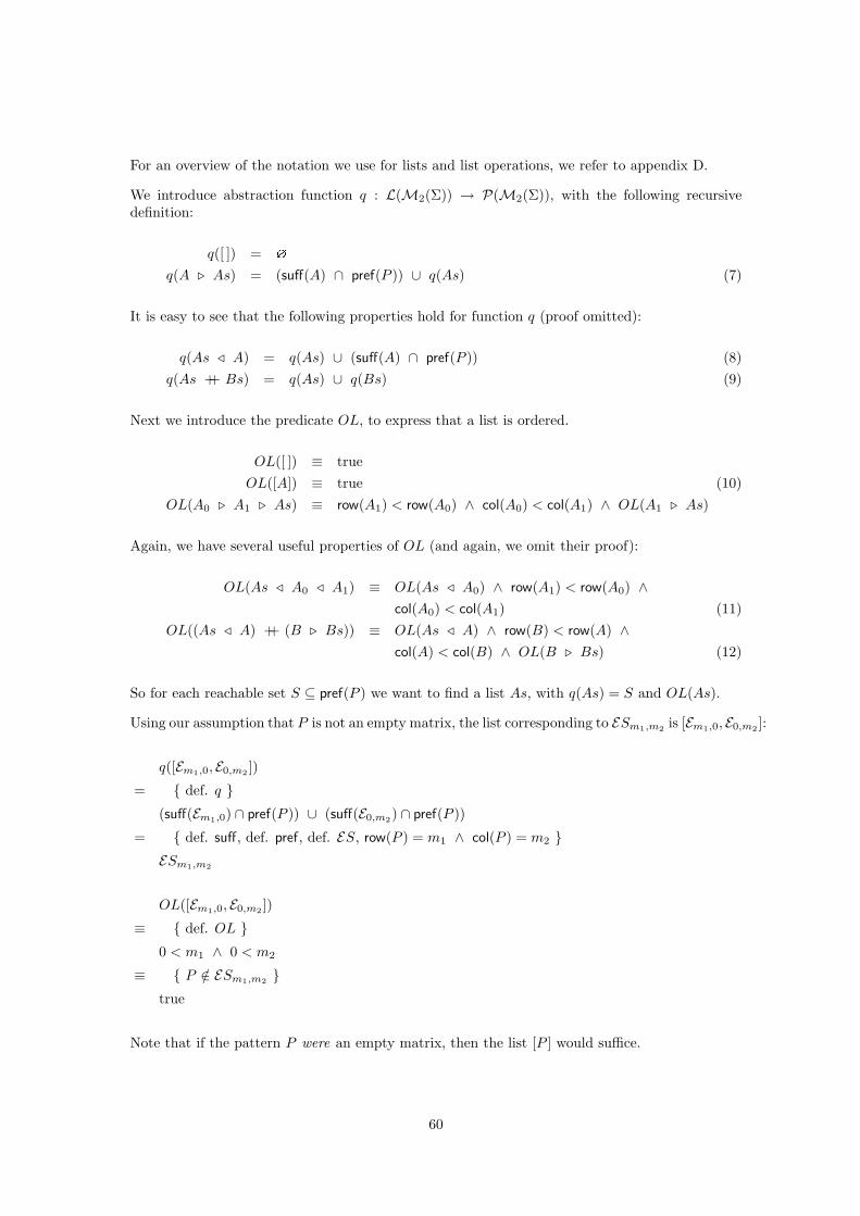
For an overview of the notation we use for lists and list operations, we refer to appendix D.

We introduce abstraction function q : L(M2(Σ)) → P(M2(Σ)), with the following recursivedefinition:

q([ ]) = ?

q(A . As) = (suff(A) ∩ pref(P )) ∪ q(As) (7)

It is easy to see that the following properties hold for function q (proof omitted):

q(As / A) = q(As) ∪ (suff(A) ∩ pref(P )) (8)q(As ++ Bs) = q(As) ∪ q(Bs) (9)

Next we introduce the predicate OL, to express that a list is ordered.

OL([ ]) ≡ trueOL([A]) ≡ true (10)

OL(A0 . A1 . As) ≡ row(A1) < row(A0) ∧ col(A0) < col(A1) ∧ OL(A1 . As)

Again, we have several useful properties of OL (and again, we omit their proof):

OL(As / A0 / A1) ≡ OL(As / A0) ∧ row(A1) < row(A0) ∧col(A0) < col(A1) (11)

OL((As / A) ++ (B . Bs)) ≡ OL(As / A) ∧ row(B) < row(A) ∧col(A) < col(B) ∧ OL(B . Bs) (12)

So for each reachable set S ⊆ pref(P ) we want to find a list As, with q(As) = S and OL(As).

Using our assumption that P is not an empty matrix, the list corresponding to ESm1,m2 is [Em1,0, E0,m2 ]:

q([Em1,0, E0,m2 ])

= { def. q }(suff(Em1,0) ∩ pref(P )) ∪ (suff(E0,m2) ∩ pref(P ))

= { def. suff, def. pref, def. ES, row(P ) = m1 ∧ col(P ) = m2 }ESm1,m2

OL([Em1,0, E0,m2 ])

≡ { def. OL }0 < m1 ∧ 0 < m2

≡ { P /∈ ESm1,m2 }true

Note that if the pattern P were an empty matrix, then the list [P ] would suffice.

60

6.3.1 Precomputation algorithm structure

Now what remains is to find an algorithm to compute a list corresponding to δ(Q,R, σ), giventhe lists corresponding to Q and R and the symbol σ. More formally, we initially have twolists Bs,Cs ∈ L(pref(P )) with:

q(Bs) = QOL(Bs)q(Cs) = ROL(Cs)

We now want to compute a list Ds ∈ L(pref(P )), satisfying:

q(Ds) = δ(Q,R, σ)OL(Ds)

We introduce the following invariants:

P0 : q(Ds) ∪ δ(q(Bs), q(Cs), σ) = δ(Q, R, σ)P1 : OL(Bs)P2 : OL(Cs)P3 : OL(Ds)

Initially, we can choose Ds = [ ]. Invariants P1, P2 and P3 then all hold trivially; ad P0:

q([ ]) ∪ δ(q(Bs), q(Cs), σ)

= { def. q }δ(q(Bs), q(Cs), σ)

= { q(Bs) = Q, q(Cs) = R }δ(Q, R, σ)

We can terminate the computation when Bs = [ ] ∨ Cs = [ ]:

q(Ds) ∪ δ(q([ ]), q(Cs), σ)

= { (7) (def. q) }q(Ds) ∪ δ(?, q(Cs), σ)

= { def. δ }q(Ds) ∪ ESm1,m2

q(Ds) ∪ δ(q(Bs), q([ ]), σ)

= { def. q }q(Ds) ∪ δ(q(Bs),?, σ)

= { def. δ }q(Ds) ∪ ESm1,m2

61

So after termination of the algorithm we have: q(Ds) ∪ ESm1,m2 = δ(Q, R, σ). Then we still needto ensure that Ds also represents ESm1,m2 . There are two possible cases: Ds = [ ] and Ds 6= [ ].

• If Ds = [ ] we can obviously conclude: ESm1,m2 * q(Ds). We have already seen that in thatcase (since we assumed that P is not an empty matrix), ESm1,m2 can be represented by thelist [Em1,0, E0,m2 ], so we can then simply write Ds := [Em1,0, E0,m2 ].

• If Ds 6= [ ], then we can write Ds as D′ . Ds′, but also as Ds′′ / D′′. We make the followingnote:

ESm1,m2 ⊆ q(Ds)

≡ { def. ES, property ⊆ }ESm1,0 ⊆ q(Ds) ∧ ES0,m2 ⊆ q(Ds)

ESm1,0 ⊆ q(D′ . Ds′)

≡ { (7) (def. q), property ∪, ∩ }ESm1,0 ⊆ (suff(D′) ∩ pref(P )) ∪ q(Ds′)

⇐ { set calculus }ESm1,0 ⊆ suff(D′) ∧ ESm1,0 ⊆ pref(P )

≡ { def. pref, row(P ) = m1 }ESm1,0 ⊆ suff(D′)

≡ { def. ES, def. suff }m1 ≤ row(D′)

If this does not hold, we need to replace Ds by Em1,0 . Ds:

ESm1,0

= { def. ES , def. suff }suff(Em1,0)

= { row(P ) = m1 }suff(Em1,0) ∩ pref(P )

⊆ { set calculus }(suff(Em1,0) ∩ pref(P )) ∪ q(D′ . Ds′)

= { def. q }q(Em1,0 . D′ . Ds′)

OL(Em1,0 . D′ . Ds′)

≡ { (10) (def. OL) }row(D′) < m1 ∧ 0 < col(D′) ∧ OL(D′ . Ds′)

≡ { row(D′) < m1, OL(D′ . Ds′) }0 < col(D′)

We still need to be sure that 0 < col(D′) holds. In the remainder of the derivation of ouralgorithm we will see that this is not a problem, since we will only add nonempty matricesto Ds.

62

The observation for ES0,m2 ⊆ q(Ds′′ / D′′) is completely symmetrical; instead of the defini-tions of q and OL we can use properties (8) and (11). We conclude that if col(D′′) < m2,we need to replace Ds by Ds / E0,m2 .

So in conclusion, after termination we need to add the following program fragment:

if Ds = [ ] → Ds := [Em1,0, E0,m2 ][] Ds :: D′ . Ds′ ∧ Ds :: Ds′′ / D′′ →

if row(D′) < m1 → Ds := Em1,0 . Ds[] m1 ≤ row(D′) → skipfi;if col(D′′) < m2 → Ds := Ds / E0,m2

[] m2 ≤ col(D′′) → skipfi

f i

So we have seen initialisation and termination of our algorithm; what remains is the updateof Bs, Cs and Ds. As we have seen, the algorithm terminates when Bs or Cs is empty, so we canassume Bs = B′ . Bs′ and Cs = C ′ . Cs′, for some B′, C ′ ∈M2(Σ) and Bs′, Cs′ ∈ L(pref(P )).We will examine the following cases:

0. row(B′) + 1 = row(C ′) ∧ col(B′) = col(C ′) + 1 ∧ P [row(B′), col(C ′)] = σ;

1. row(C ′) < row(B′) + 1;

2. row(B′) + 1 < row(C ′);

3. row(B′) + 1 = row(C ′) ∧ col(C ′) + 1 < col(B′);

4. row(B′) + 1 = row(C ′) ∧ col(B′) < col(C ′) + 1;

5. row(B′) + 1 = row(C ′) ∧ col(B′) = col(C ′) + 1 ∧ P [row(B′), col(C ′)] 6= σ.

6.3.2 Case analysis

Case 0

The first case is: row(B′) + 1 = row(C ′) ∧ col(B′) = col(C ′) + 1 ∧ P [row(B′), col(C ′)] = σ.Informally, this is the case where a combination of B′, C ′ and σ actually occurs as a prefix of P .

First we examine the left-hand side of invariant P0:

q(Ds) ∪ δ(q(B′ . Bs′), q(C ′ . Cs′), σ)

= { def. δ }q(Ds) ∪ 〈set A, b, c : SIZE (A, b, c) ∧

[A b

]∈ q(B′ . Bs′) ∧[

Ac

]∈ q(C ′ . Cs′) ∧ σ = P [row(A), col(A)] :

[A bc σ

]〉 ∪ ESm1,m2

= { (7) (def. q) }q(Ds) ∪ 〈set A, b, c : SIZE (A, b, c) ∧

[A b

]∈ (suff(B′) ∩ pref(P )) ∪ q(Bs′) ∧[

Ac

]∈ (suff(C ′) ∩ pref(P )) ∪ q(Cs′) ∧ σ = P [row(A), col(A)] :

[A bc σ

]〉 ∪

63

ESm1,m2

= { set calculus }q(Ds) ∪ 〈set A, b, c : SIZE (A, b, c) ∧

[A b

]∈ suff(B′) ∩ pref(P ) ∧[

Ac

]∈ (suff(C ′) ∩ pref(P )) ∪ q(Cs′) ∧ σ = P [row(A), col(A)] :

[A bc σ

]〉 ∪

〈set A, b, c : SIZE (A, b, c) ∧[

A b]∈ (suff(B′) ∩ pref(P )) ∪ q(Bs′) ∧[

Ac

]∈ suff(C ′) ∩ pref(P ) ∧ σ = P [row(A), col(A)] :

[A bc σ

]〉 ∪

〈set A, b, c : SIZE (A, b, c) ∧[A b

]∈ q(Bs′) ∧

[Ac

]∈ q(Cs′) ∧ σ = P [row(A), col(A)] :[

A bc σ

]〉 ∪ ESm1,m2

= { def. δ }q(Ds) ∪ 〈set A, b, c : SIZE (A, b, c) ∧

[A b

]∈ suff(B′) ∩ pref(P ) ∧[

Ac

]∈ (suff(C ′) ∩ pref(P )) ∪ q(Cs′) ∧ σ = P [row(A), col(A)] :

[A bc σ

]〉 ∪

〈set A, b, c : SIZE (A, b, c) ∧[

A b]∈ (suff(B′) ∩ pref(P )) ∪ q(Bs′) ∧[

Ac

]∈ suff(C ′) ∩ pref(P ) ∧ σ = P [row(A), col(A)] :

[A bc σ

]〉 ∪

δ(q(Bs′), q(Cs′), σ)

To further simplify this complex expression, we make the following observation, for matrices A, b

and c with SIZE (A, b, c) and[

Ac

]∈ R:

[A b

]∈ suff(B′) ∩ pref(P )

⇒ { definition suff }row(

[A b

]) ≤ row(B′) ∧ col(

[A b

]) ≤ col(B′)

≡ { definition row, col }row(A) ≤ row(B′) ∧ col(A) < col(B′)

≡ { row(B′) + 1 = row(C ′) ∧ col(B′) = col(C ′) + 1 }row(A) < row(C ′) ∧ col(A) ≤ col(C ′)

≡ { def. row, col }

row([

Ac

]) ≤ row(C ′) ∧ col(

[Ac

]) ≤ col(C ′)

≡ {[

Ac

], C ′ ∈ R, therefore

[Ac

], C ′ ∈ pref(P ) }[

Ac

]∈ pref(C ′)

⇒ { theorem 6.5;[

Ac

], C ′ ∈ R; R is a reachable set }[

Ac

]∈ suff(C ′)

≡ {[

Ac

]∈ pref(P ) }

64

[Ac

]∈ suff(C ′) ∩ pref(P )

And symmetrically, with[

A b]∈ Q:

[Ac

]∈ suff(C ′) ∩ pref(P )

⇒ { def. suff, row, col }row(A) < row(C ′) ∧ col(A) ≤ col(C ′)

≡ { row(B′) + 1 = row(C ′) ∧ col(B′) = col(C ′) + 1 }row(A) ≤ row(B′) ∧ col(A) < col(B′)

≡ { def. row, col }row(

[A b

]) ≤ row(B′) ∧ col(

[A b

]) ≤ col(B′)

≡ {[

A b], B′ ∈ Q, therefore

[A b

], B′ ∈ pref(P ) }[

A b]∈ pref(B′)

⇒ { theorem 6.5;[

A b], B′ ∈ Q; Q is a reachable set }[

A b]∈ suff(B′)

≡ {[

A b]∈ pref(P ) }[

A b]∈ suff(B′) ∩ pref(P )

So we know that in this case the left hand side of P0 is equal to:

q(Ds) ∪ 〈set A, b, c : SIZE (A, b, c) ∧[

A b]∈ suff(B′) ∩ pref(P ) ∧[

Ac

]∈ suff(C ′) ∩ pref(P ) ∧ σ = P [row(A), col(A)] :

[A bc σ

]〉 ∪

δ(q(Bs′), q(Cs′), σ)

Again, for the following derivation, we look at a subexpression, assuming we have matrices A, band c with SIZE (A, b, c):

[A b

]∈ suff(B′) ∩ pref(P ) ∧

[Ac

]∈ suff(C ′) ∩ pref(P ) ∧ σ = P [row(A), col(A)]

≡ { prop. ∩ }[A b

]∈ suff(B′) ∧

[Ac

]∈ suff(C ′) ∧

[A b

]∈ pref(P ) ∧

[Ac

]∈ pref(P ) ∧

σ = P [row(A), col(A)]

≡ { property pref }[A b

]∈ suff(B′) ∧

[Ac

]∈ suff(C ′) ∧

[A bc σ

]∈ pref(P )

≡ { B′, C ′ ∈ pref(P ) }[A b

]∈ suff(P [0 .. row(B′))[0 .. col(B′))) ∧[

Ac

]∈ suff(P [0 .. row(C ′))[0 .. col(C ′))) ∧

[A bc σ

]∈ pref(P )

≡ { row(B′) + 1 = row(C ′), col(B′) = col(C ′) + 1 }

65

[A b

]∈ suff(P [0 .. row(C ′)− 1)[0 .. col(B′))) ∧[

Ac

]∈ suff(P [0 .. row(C ′))[0 .. col(B′)− 1)) ∧

[A bc σ

]∈ pref(P )

≡ { P [row(B′), col(C ′)] = σ; property suff }[A bc σ

]∈ suff(P [0 .. row(C ′))[0 .. col(B′))) ∧

[A bc σ

]∈ pref(P )

≡ { property ∩ }[A bc σ

]∈ suff(P [0 .. row(C ′))[0 .. col(B′))) ∩ pref(P )

Now we can get back to our main derivation:

q(Ds) ∪ 〈set A, b, c : SIZE (A, b, c) ∧[A bc σ

]∈ suff(P [0 .. row(C ′))[0 .. col(B′))) ∩ pref(P ) :

[A bc σ

]〉 ∪

δ(q(Bs′), q(Cs′), σ)

= { def. SIZE }q(Ds) ∪ 〈set A, b, c : row(A) < m1 ∧ col(A) < m2 ∧

row(b) = row(A) ∧ col(b) = 1 ∧ row(c) = 1 ∧ col(c) = col(A) ∧[A bc σ

]∈ suff(P [0 .. row(C ′))[0 .. col(B′))) ∩ pref(P ) :

[A bc σ

]〉 ∪

δ(q(Bs′), q(Cs′), σ)

= { row(C ′) ≤ m1, col(B′) ≤ m2 }q(Ds) ∪ 〈set A : A /∈ ES ∧ A ∈ suff(P [0 .. row(C ′))[0 .. col(B′))) ∩ pref(P ) : A〉 ∪

δ(q(Bs′), q(Cs′), σ)

= { row(C ′) ≤ m1 and col(B′) ≤ m2, therefore ESrow(C′),col(B′) ∈ δ(q(Bs′), q(Cs′), σ) }q(Ds) ∪ 〈set A : A ∈ suff(P [0 .. row(C ′))[0 .. col(B′))) ∩ pref(P ) : A〉 ∪δ(q(Bs′), q(Cs′), σ)

= { set calculus }q(Ds) ∪ suff(P [0 .. row(C ′))[0 .. col(B′))) ∩ pref(P ) ∪ δ(q(Bs′), q(Cs′), σ)

= { property (8) }q(Ds / P [0 .. row(C ′))[0 .. col(B′))) ∪ δ(q(Bs′), q(Cs′), σ)

This leads to the following program fragment:

Ds := Ds / P [0 .. row(C ′))[0 .. col(B′));Bs := Bs′;Cs := Cs′

Of course we still need to verify that this does not violate the other invariants P1, P2 and P3.From (10), the definition of OL, it is not hard to see that P1 and P2 still hold after removing thefirst elements of Bs and Cs. For P3, there are two relevant cases: Ds = [ ] and Ds = Ds′ / D′.

OL([ ] / Ds)

≡ { (10) }true

66

OL(Ds′ / D′ / P [0 .. row(C ′))[0 .. col(B′)))

≡ { property (11) }OL(Ds′ / D′) ∧ row(P [0 .. row(C ′))[0 .. col(B′))) < row(D′) ∧

col(D′) < col(P [0 .. row(C ′))[0 .. col(B′)))

≡ { Ds′ / D′ = Ds, P2; def. row, col }row(C ′) < row(D′) ∧ col(D′) < col(B′)

≡ { idempotence of ∧, row(B′) = row(C ′) + 1, col(B′) + 1 = col(C ′) }row(B′) + 1 < row(D′) ∧ col(D′) < col(B′) ∧

row(C ′) < row(D′) ∧ col(D′) < col(C ′) + 1

≡ { •OLr(Ds′ / D′, B′ . Bs′), OLc(Ds′ / D′, C ′ . Cs′) }true

We introduce the following two extra invariants:

P4 : OLr(Ds,Bs)P5 : OLc(Ds, Cs)

Predicates OLr and OLc are defined as follows:

OLr([ ], As) ≡ trueOLr(Es, [ ]) ≡ true (13)

OLr(Es / E,A . As) ≡ row(A) + 1 < row(E) ∧ col(E) < col(A)

OLc([ ], As) ≡ trueOLc(Es, [ ]) ≡ true (14)

OLc(Es / E, A . As) ≡ row(A) < row(E) ∧ col(E) < col(A) + 1

From these definitions we can see that extra invariants P4 and P5 hold initially, since [ ] is theinitial value of Ds. It should also be obvious that OLr(Ds / P [0 .. row(C ′))[0 .. col(B′)), Bs′)follows from row(B′) + 1 = row(C ′) and OL(B′ . Bs′) (which is invariant P1). Symmetrically,we know that OLc(Ds / P [0 .. row(C ′))[0 .. col(B′)), Cs′) follows from col(B′) = col(C ′) + 1and OL(C ′ . Cs′).

In case 0 we have seen how to update Ds, Bs and Cs when a combination of B′, C ′ and σ actuallyoccurs as a prefix of the text. The remaining cases are the various situations in which there is noway to combine B′, C ′ and σ into such a prefix.

Case 1

Here we will take a look at the case where row(C ′) < row(B′) + 1. Again we start by examiningthe left-hand side of invariant P0.

q(Ds) ∪ δ(q(B′ . Bs′), q(C ′ . Cs′), σ)

= { definition δ }q(Ds) ∪ 〈set A, b, c : SIZE (A, b, c) ∧

[A b

]∈ q(B′ . Bs′) ∧

67

[Ac

]∈ q(C ′ . Cs′) ∧ σ = P [row(A), col(A)] :

[A bc σ

]〉 ∪

ESm1,m2

Here too, we will take a look at a subexpression in detail. We assume we have A, b and csatisfying SIZE (A, b, c) and we derive:

[Ac

]∈ q(C ′ . Cs′)

≡ { definition q }[Ac

]∈ (suff(C ′) ∩ pref(P )) ∪ q(Cs′)

⇒ { property suff, invariant P2: OL(C ′ . Cs′) }

row([

Ac

]) ≤ row(C ′)

⇒ { row(C ′) < row(B′) + 1 }

row([

Ac

]) < row(B′) + 1

≡ { definition row }row(

[A b

]) < row(B′)

⇒ { property of functions }[A b

]6= B′

We conclude:

[A b

]∈ q(B′ . Bs′)

≡ { (7) (definition q) }[A b

]∈ (suff(B′) ∩ pref(P )) ∪ q(Bs′)

≡ {[

A b]6= B′ }[

A b]∈ ((suff(B′) ∩ pref(P )) \ {B′}) ∪ q(Bs′)

≡ { • spec. r }[A b

]∈ q(r(B′)) ∪ q(Bs′)

Here we introduce function r : pref(P ) → L(pref(P )), which, given A ∈ pref(P ), returns the listof maximal elements of (suff(A) ∩ pref(P )) \ {A}. In other words, r(A) is the list satisfying thefollowing properties:

q(r(A)) = (suff(A) ∩ pref(P )) \ {A}OL(r(A))

The values of function r can be precomputed for every prefix of P . We will get back to this later,in section 6.3.4; for now we just assume we have such a function r.

We can now conclude that the left-hand-side of P0 is in this case equal to:

68

q(Ds) ∪ 〈set A, b, c : SIZE (A, b, c) ∧[

A b]∈ q(r(B′)) ∪ q(Bs′) ∧[

Ac

]∈ q(C ′ . Cs′) ∧ σ = P [row(A), col(A)] :

[A bc σ

]〉 ∪ ESm1,m2

This suggests that we might want to replace Bs by r(B′) ++ Bs′. That would be sufficientto ensure that P0 holds again. However, there is no way to guarantee that OL(r(B′) ++ Bs′)and OLr(Ds, r(B′) ++ Bs′) hold.

For example, r(B′) may very well contain a matrix R that is a strict suffix of an element of Bs′.Then R is not a maximal element of q(r(B′) ++ Bs′) and that means that OL(r(B′) ++ Bs′) doesnot hold. However, in this case we also know that every matrix in suff(R) is already representedby Bs′, so we can simply omit matrix R.

Because of invariant OL(B′ . Bs′) and OL(r(B′)), we know that the elements of r(B′) that arealso a suffix of some element of Bs′ form a tail of r(B′). So eliminating these elements of r(B′)consists of a linear search starting at the last element of r(B′), eliminating every element untilone is found that is not a suffix of some element of Bs′.

Similarly, we cannot guarantee that OLr(Ds, r(B′) ++ Bs′) holds, but we do know that we canomit the matrices in r(B’) which have already been considered in the computation of Ds. We alsoknow that those matrices occur at the beginning of r(B′).

First we will focus on OL and try to compute a list Rs, such that q(Rs ++Bs′) = q(r(B′) ++Bs′),but also OL(Rs ++Bs′). We distinguish two possible cases for Bs′: Bs′ = [ ] and Bs′ 6= [ ].

• If Bs′ = [ ], we can make the following observation:

OL(r(B′) ++ [ ])

≡ { definition ++ }OL(r(B′))

≡ { specification r }true

So in this case, the choice Rs = r(B′) does suffice.

• If Bs′ is not empty, we can write it as B′′ . Bs′′, for some matrix B′′ and list Bs′′. Tocompute a list Rs satisfying q(Rs ++Bs′) = q(r(B′) ++Bs′) and OL(Rs ++Bs′), we initiallychoose Rs = r(B′) and introduce the following invariants:

Q0 OL(Rs)Q1 q(Rs ++Bs′) = q(r(B′) ++Bs′)

Concerning termination, we again look at two different cases: Rs = [ ] and Rs 6= [ ].

– Assuming Rs = [ ], we derive:

OL([ ] ++(B′′ . Bs′′))

≡ { definition ++ }OL(B′′ . Bs′′)

⇐ { definition OL }OL(B′ . B′′ . Bs′′)

≡ { P1 }true

69

So if Rs is empty, we can terminate this computation.

– If R 6= [ ], we can write Rs as Rs′ / R′.

OL((RS′ / R′) ++ (B′′ . Bs′′))

≡ { property (12) }OL(RS′ / R′) ∧ OL(B′′ . Bs′′) ∧ row(B′′) < row(R′) ∧ col(R′) < col(B′)

≡ { Q0, P1 }row(B′′) < row(R′) ∧ col(R′) < col(B′′)

⇐ { R′ ∈ r(B′), therefore R′ ∈ suff(B′) and col(R′) ≤ col(B′) }row(B′′) < row(R′) ∧ col(B′) < col(B′′)

≡ { P1 : OL(B′ . B′′ . Bs′′) }row(B′′) < row(R′)

If row(B′′) < row(R′), we can terminate the computation as well. Otherwise, we canderive:

row(R′) ≤ row(B′′)

⇒ { col(R′) < col(B′′) (see previous derivation); R′, B′′ ∈ pref(P ) }R′ ∈ pref(B′′)

⇒ { R′, B′′ ∈ Q, theorem 6.5 }R′ ∈ suff(B′′)

≡ { property suff }suff(R′) ⊆ suff(B′)

⇒ { set calculus }suff(R′) ∩ pref(P ) ⊆ suff(B′) ∩ pref(P )

We can use this in the following derivation, which starts with the left-hand side ofinvariant Q1:

q((Rs′ / R′) ++ (B′′ . Bs′′))

= { (7), (8) and (9) }q(Rs′) ∪ (suff(R′) ∩ pref(P )) ∪ (suff(B′′) ∩ pref(P )) ∪ q(Bs′′)

= { suff(R′) ∩ pref(P ) ⊆ suff(B′) ∩ pref(P ) }q(Rs′) ∪ (suff(B′′) ∩ pref(P )) ∪ q(Bs′′)

= { (7), (9) }q(Rs′ ++ (B′′ . Bs′′))

So the algorithm to compute Rs becomes:

Rs := r(B′);if Bs′ = [ ] → skip[] Bs′ :: B′′ . Bs′′ →

do Rs :: Rs′ / R′ cand row(R′) < row(B′′) →Rs := Rs′

odfi

70

Now we still need to establish OLr(Ds,Rs ++ Bs′). We do this by an algorithm similar to theone presented above. We will only eliminate elements of Rs, so we can be sure that this algorithmwill not falsify OL(Rs ++ Bs′).

Again, we will consider two cases: Ds = [ ] and Ds 6= [ ].

• If Ds = [ ], we can simply observe:

OLr([ ], Rs ++Bs′)

≡ { (13) }true

• If Ds 6= [ ], it is of the form Ds′ / D′. We distinguish two different cases for the structureof Rs.

– If Rs = [ ], we get:

OLr(Ds′ / D′, [ ] ++Bs′)

≡ { definition ++ }OLr(Ds′ / D′, Bs′)

≡ { P1, P4 }true

– If Rs 6= [ ], we can write Rs as R′ . Rs′. We get the following derivation:

OLr(Ds′ / D′, (R′ . Rs′) ++Bs′)

≡ { (13) }row(R′) + 1 < row(D′) ∧ col(D′) < col(R′)

⇐ { R′ ∈ suff(B′) }row(B′) + 1 < row(D′) ∧ col(D′) < col(R′)

≡ { P4 }col(D′) < col(R′)

If this does not hold (that is, in the case that col(R′) ≤ col(D′)), we want to eliminate R′

from the list, much like in the previous algorithm. We will now show that this does notfalsify P0, with Bs replaced by Rs ++Bs′. We get the following derivation:

q(Ds′ / D′) ∪ δ(q(R′ . Rs′ ++Bs′), q(C ′ . Cs′), σ)

= { definition δ }q(Ds′ / D′) ∪〈set A, b, c : SIZE (A, b, c) ∧

[A b

]∈ q(R′ . Rs′ ++Bs′) ∧[

Ac

]∈ q(C ′ . Cs′) ∧ σ = P [row(A), col(A)] :

[A bc σ

]〉 ∪

ESm1,m2

= { domain split, definition δ }q(Ds′ / D′) ∪〈set A, b, c : SIZE (A, b, c) ∧

[A b

]∈ suff(R′) ∩ pref(P ) ∧[

Ac

]∈ q(C ′ . Cs′) ∧ σ = P [row(A), col(A)] :

[A bc σ

]〉 ∪

71

δ(q(Rs′ ++Bs′), q(C ′ . Cs′), σ)

= { • see below }q(Ds′ / D′) ∪ δ(q(Rs′ ++Bs′), q(C ′ . Cs′), σ)

For the step that we still need to prove, we assume we have matrices A, b and c, whichsatisfy:

SIZE (A, b, c) ∧[

A b]∈ suff(R′) ∩ pref(P ) ∧[

Ac

]∈ q(C ′ . Cs′) ∧ σ = P [row(A), col(A)]

We get the following derivation:[A b

]∈ suff(R′) ∩ pref(P )

⇒ { property suff }row(

[A b

]) ≤ row(R′) ∧ col(

[A b

]) ≤ col(R′)

⇒ { col(R′) ≤ col(D′) }row(

[A b

]) ≤ row(R′) ∧ col(

[A b

]) ≤ col(D′)

⇒ { R′ ∈ suff(B′) }row(

[A b

]) ≤ row(B′) ∧ col(

[A b

]) ≤ col(D′)

⇒ { P4 : OLr(Ds′ / D′, B′ . Bs′) }row(

[A b

]) < row(D′)− 1 ∧ col(

[A b

]) ≤ col(D′)

≡ { def. row, col }

row([

A bc σ

]) < row(D′) ∧ col(

[A bc σ

]) ≤ col(D′)

⇒ {[

A b]∈ pref(P ),

[Ac

]∈ pref(P ) and σ = P [row(A), col(A)],

therefore:[

A bc σ

]∈ pref(P ); D′ ∈ pref(P )

}[A bc σ

]∈ pref(D′)

⇒ {[

A bc σ

], D′ ∈ δ(Q, R, σ); theorem 6.5 }[

A bc σ

]∈ suff(D′)

≡ {[

A b]∈ pref(P ),

[Ac

]∈ pref(P ) and σ = P [row(A), col(A)] }[

A bc σ

]∈ suff(D′) ∩ pref(P )

⇒ { set calculus }[A bc σ

]∈ q(Ds′) ∪ (suff(D′) ∩ pref(P ))

≡ { property (8) }[A bc σ

]∈ q(Ds′ / D′)

72

So the following program fragment suffices:

if Ds = [ ] → skip[] Ds :: Ds′ / D′ →

do Rs :: R′ . Rs′ cand col(R′) ≤ col(D′) →Rs := Rs′

odfi

Case 2

We will now examine the case: row(B′) + 1 < row(C ′).

q(Ds) ∪ δ(q(B′ . Bs′), q(C ′ . Cs′), σ)

= { definition δ }q(Ds) ∪ 〈set A, b, c : SIZE (A, b, c) ∧

[A b

]∈ q(B′ . Bs′) ∧[

Ac

]∈ q(C ′ . Cs′) ∧ σ = P [row(A), col(A)] :

[A bc σ

]〉 ∪

ESm1,m2

Here, we can derive, somewhat symmetrically to case 1:

[A b

]∈ q(B . Bs′)

≡ { (7) (definition q) }[A b

]∈ (suff(B′) ∩ pref(P )) ∪ q(Bs′)

⇒ { OL(B′ . Bs′) }row(

[A b

]) ≤ row(B′)

⇒ { row(B′) + 1 < row(C ′) }row(

[A b

]) < row(C ′)− 1

≡ { def. row }

row([

Ac

]) < row(C ′)

⇒ { property functions }[Ac

]6= C ′

And we can conclude:

[Ac

]∈ q(C ′ . Cs′)

≡ { (7) (definition q) }[Ac

]∈ (suff(C ′) ∩ pref(P )) ∪ q(Cs′)

≡ {[

Ac

]6= C ′ }

73

[Ac

]∈ ((suff(C ′) ∩ pref(P )) \ {C ′}) ∪ q(Cs′)

≡ { specification r }[Ac

]∈ r(C ′) ∪ q(Cs′)

To ensure that P2 and P5 hold, we need to eliminate certain elements of r(C ′). The derivation ofsuch an algorithm is symmetrical to case 1 and will be omitted here; instead we just present theentire algorithm immediately.

Rs := r(C ′);if Cs′ = [ ] → skip[] Cs′ :: C ′′ . Cs′′ →

do Rs :: Rs′ / R′ cand row(R′) ≤ row(C ′′) →Rs := Rs′

odfi;if Ds = [ ] → skip[] Ds :: Ds′ / D′ →

do Rs :: R′ / Rs′ cand col(R′) < col(D′) →Rs := Rs′

odfi

After computing Rs using this algorithm, we can safely replace Cs with Rs ++Cs′.

Case 3

Here we examine the case: row(B′) + 1 = row(C ′) ∧ col(C ′) + 1 < col(B′).

Then:

q(Ds) ∪ δ(q(B′ . Bs′), q(C ′ . Cs′), σ)

= { definition δ }q(Ds) ∪ 〈set A, b, c : SIZE (A, b, c) ∧

[A b

]∈ q(B′ . Bs′) ∧[

Ac

]∈ q(C ′ . Cs′) ∧ σ = P [row(A), col(A)] :

[A bc σ

]〉 ∪

ESm1,m2

As in case 1, we can now show:[

Ac

]∈ q(C ′ . Cs′) ⇒

[A b

]6= B′ (for A, b and c

satisfying SIZE (A, b, c)).

[Ac

]∈ q(C ′ . Cs′)

≡ { (7) }[Ac

]∈ (suff(C ′) ∩ pref(P )) ∪ Cs′

≡ { property ∪ }

74

[Ac

]∈ suff(C ′) ∩ pref(P ) ∨

[Ac

]∈ Cs′

We proceed to show that both disjuncts imply[

A b]6= B′.

•[

Ac

]∈ suff(C ′) ∩ pref(P )

⇒ { property suff }

col([

Ac

]) ≤ col(C ′)

≡ { definition col }col(

[A b

]) ≤ col(C ′) + 1

⇒ { col(C ′) + 1 < col(B′) }col(

[A b

]) < col(B′)

⇒ { property functions }[A b

]6= B′

•[

Ac

]∈ q(Cs′)

⇒ { P2: OL(C ′ . Cs′) }

row([

Ac

]) < row(C ′)

≡ { row(B′) + 1 = row(C ′) }

row([

Ac

]) < row(B′) + 1

≡ { definition row }row(

[A b

]) < row(B′)

⇒ { property functions }[A b

]6= B′

Now we can draw the same conclusion as in case 1:

[A b

]∈ q(B′ . Bs′)

≡ { (7) }[A b

]∈ (suff(B′) ∩ pref(P )) ∪ q(Bs′)

≡ {[

A b]6= B′ }[

A b]∈ ((suff(B′) ∩ pref(P )) \ {B′}) ∪ q(Bs′)

≡ { spec. r }[A b

]∈ q(r(B′)) ∪ q(Bs′)

Note that in the rest of the derivation in case 1 we never use the assumption row(C ′) ≤ row(B′).That means that we can now use the same algorithm for computing a list Rs from list r(B′), suchthat we can replace Bs by Rs ++Bs′.

75

Case 4

Case 4 is: row(B′) + 1 = row(C ′) ∧ col(B′) < col(C ′) + 1. We derive:

q(Ds) ∪ δ(q(B′ . Bs′), q(C ′ . Cs′), σ)

= { definition δ, (7) (definition q) }q(Ds) ∪ 〈set A, b, c : SIZE (A, b, c) ∧

[A b

]∈ q(B′ . Bs′) ∧[

Ac

]∈ q(C ′ . Cs′) ∧ σ = P [row(A), col(A)] :

[A bc σ

]〉 ∪

ESm1,m2

For A, b and c satisfying SIZE (A, b, c), we derive:

[A b

]∈ q(B′ . Bs′)

≡ { (7), property ∩ }[A b

]∈ suff(B′) ∩ pref(P ) ∨

[A b

]∈ q(Bs′)

We examine both disjuncts seperately to show that both imply[

Ac

]6= C ′:

•[

A b]∈ suff(B′) ∩ pref(P )

⇒ { property suff }col(

[A b

]) ≤ col(B′)

⇒ { col(B′) ≤ col(C ′) }col(

[A b

]) ≤ col(C ′)

≡ { definition col }

col([

Ac

]) < col(C ′)

⇒ { property functions }[Ac

]6= C ′

•[

A b]∈ q(Bs′)

⇒ { OL(B′ . Bs′) }row(

[A b

]) < row(B′)

≡ { definition row }

row([

Ac

]) < row(B′) + 1

≡ { row(B′) + 1 = row(C ′) }

row([

Ac

]) < row(C ′)

⇒ { property functions }[Ac

]6= C ′

76

Therefore we have the same conclusion as in case 2:

[Ac

]∈ q(C ′ . Cs′)

≡ { (7) }[Ac

]∈ (suff(C ′) ∩ pref(P )) ∪ q(Cs′)

≡ {[

Ac

]6= C ′ }[

Ac

]∈ ((suff(C ′) ∩ pref(P )) \ {C ′}) ∪ q(Cs′)

≡ { specification r }[Ac

]∈ r(C ′) ∪ q(Cs′)

And again, we can use the same algorithm presented in case 2 to compute a list Rs, so we canreplace Cs by Rs ++Cs′.

Case 5

Our final case is the case where the sizes of B′ and C ′ do match, but σ does not occur in the rightspot in the pattern: row(B′) + 1 = row(C ′) ∧ col(B′) = col(C ′) + 1 ∧ P [row(B′), col(C ′)] 6= σ.

q(Ds) ∪ δ(q(B′ . Bs′), q(C ′ . Cs′), σ)

= { definition δ }q(Ds) ∪ 〈set A, b, c : SIZE (A, b, c) ∧

[A b

]∈ q(B′ . Bs′) ∧[

Ac

]∈ q(C ′ . Cs′) ∧ σ = P [row(A), col(A)] :

[A bc σ

]〉 ∪

ESm1,m2

We assume we have matrices A, b and c, satisfying:

SIZE (A, b, c) ∧[

A b]∈ q(B′ . Bs′) ∧[

Ac

]∈ q(C ′ . Cs′) ∧ σ = P [row(A), col(A)]

Then the assumption P [row(B′), col(C ′)] 6= σ gives us the following:

P [row(B′), col(C ′)] 6= σ

⇒ { P [row(A), col(A)] = σ }row(A) 6= row(B′) ∨ col(A) 6= col(C ′)

We examine both of these disjuncts:

• row(A) 6= row(B′)

≡ { idempotence ∧, definition row }

77

row([

A b]) 6= row(B′) ∧ row(

[Ac

]) 6= row(B′) + 1

≡ { row(B′) + 1 = row(C ′) }

row([

A b]) 6= row(B′) ∧ row(

[Ac

]) 6= row(C ′)

⇒ { property functions }[A b

]6= B′ ∧

[Ac

]6= C ′

• col(A) 6= col(C ′)

≡ { idempotence ∧, definition col }

col([

A b]) 6= col(C ′) + 1 ∧ col(

[Ac

]) 6= col(C ′)

≡ { col(B′) = col(C ′) + 1 }

col([

A b]) 6= col(B′) ∧ col(

[Ac

]) 6= col(C ′)

⇒ { property functions }[A b

]6= B′ ∧

[Ac

]6= C ′

Using[

A b]6= B′, we can draw the same conclusion we did in case 1 and case 3:

[A b

]∈ q(B′ . Bs′)

≡ { (7) }[A b

]∈ (suff(B′) ∩ pref(P )) ∪ q(Bs′)

≡ {[

A b]6= B′ }[

A b]∈ ((suff(B′) ∩ pref(P )) \ {B′}) ∪ q(Bs′)

≡ { spec. r }[A b

]∈ q(r(B′)) ∪ q(Bs′)

However, using[

Ac

]6= C ′, the observation seen in case 2 and case 4 is also correct:

[Ac

]∈ q(C ′ . Cs′)

≡ { (7) }[Ac

]∈ (suff(C ′) ∩ pref(P )) ∪ q(Cs′)

≡ {[

Ac

]6= C ′ }[

Ac

]∈ ((suff(C ′) ∩ pref(P )) \ {C ′}) ∪ q(Cs′)

≡ { specification r }[Ac

]∈ r(C ′) ∪ q(Cs′)

78

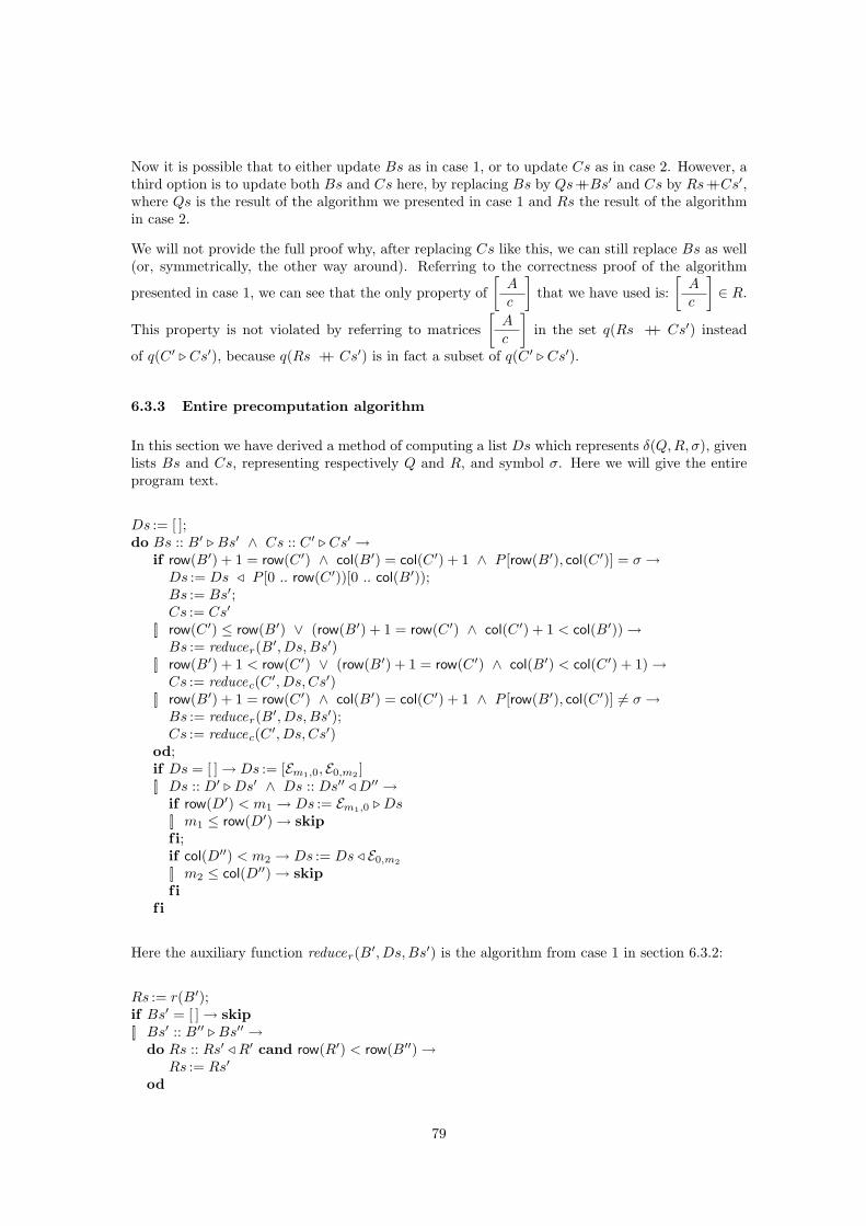
Now it is possible that to either update Bs as in case 1, or to update Cs as in case 2. However, athird option is to update both Bs and Cs here, by replacing Bs by Qs++Bs′ and Cs by Rs++Cs′,where Qs is the result of the algorithm we presented in case 1 and Rs the result of the algorithmin case 2.

We will not provide the full proof why, after replacing Cs like this, we can still replace Bs as well(or, symmetrically, the other way around). Referring to the correctness proof of the algorithm

presented in case 1, we can see that the only property of[

Ac

]that we have used is:

[Ac

]∈ R.

This property is not violated by referring to matrices[

Ac

]in the set q(Rs ++ Cs′) instead

of q(C ′ . Cs′), because q(Rs ++ Cs′) is in fact a subset of q(C ′ . Cs′).

6.3.3 Entire precomputation algorithm

In this section we have derived a method of computing a list Ds which represents δ(Q, R, σ), givenlists Bs and Cs, representing respectively Q and R, and symbol σ. Here we will give the entireprogram text.

Ds := [ ];do Bs :: B′ . Bs′ ∧ Cs :: C ′ . Cs′ →

if row(B′) + 1 = row(C ′) ∧ col(B′) = col(C ′) + 1 ∧ P [row(B′), col(C ′)] = σ →Ds := Ds / P [0 .. row(C ′))[0 .. col(B′));Bs := Bs′;Cs := Cs′

[] row(C ′) ≤ row(B′) ∨ (row(B′) + 1 = row(C ′) ∧ col(C ′) + 1 < col(B′)) →Bs := reducer(B′, Ds, Bs′)

[] row(B′) + 1 < row(C ′) ∨ (row(B′) + 1 = row(C ′) ∧ col(B′) < col(C ′) + 1) →Cs := reducec(C ′, Ds, Cs′)

[] row(B′) + 1 = row(C ′) ∧ col(B′) = col(C ′) + 1 ∧ P [row(B′), col(C ′)] 6= σ →Bs := reducer(B′, Ds, Bs′);Cs := reducec(C ′, Ds, Cs′)

od;if Ds = [ ] → Ds := [Em1,0, E0,m2 ][] Ds :: D′ . Ds′ ∧ Ds :: Ds′′ / D′′ →

if row(D′) < m1 → Ds := Em1,0 . Ds[] m1 ≤ row(D′) → skipfi;if col(D′′) < m2 → Ds := Ds / E0,m2

[] m2 ≤ col(D′′) → skipfi

f i

Here the auxiliary function reducer(B′, Ds,Bs′) is the algorithm from case 1 in section 6.3.2:

Rs := r(B′);if Bs′ = [ ] → skip[] Bs′ :: B′′ . Bs′′ →

do Rs :: Rs′ / R′ cand row(R′) < row(B′′) →Rs := Rs′

od

79

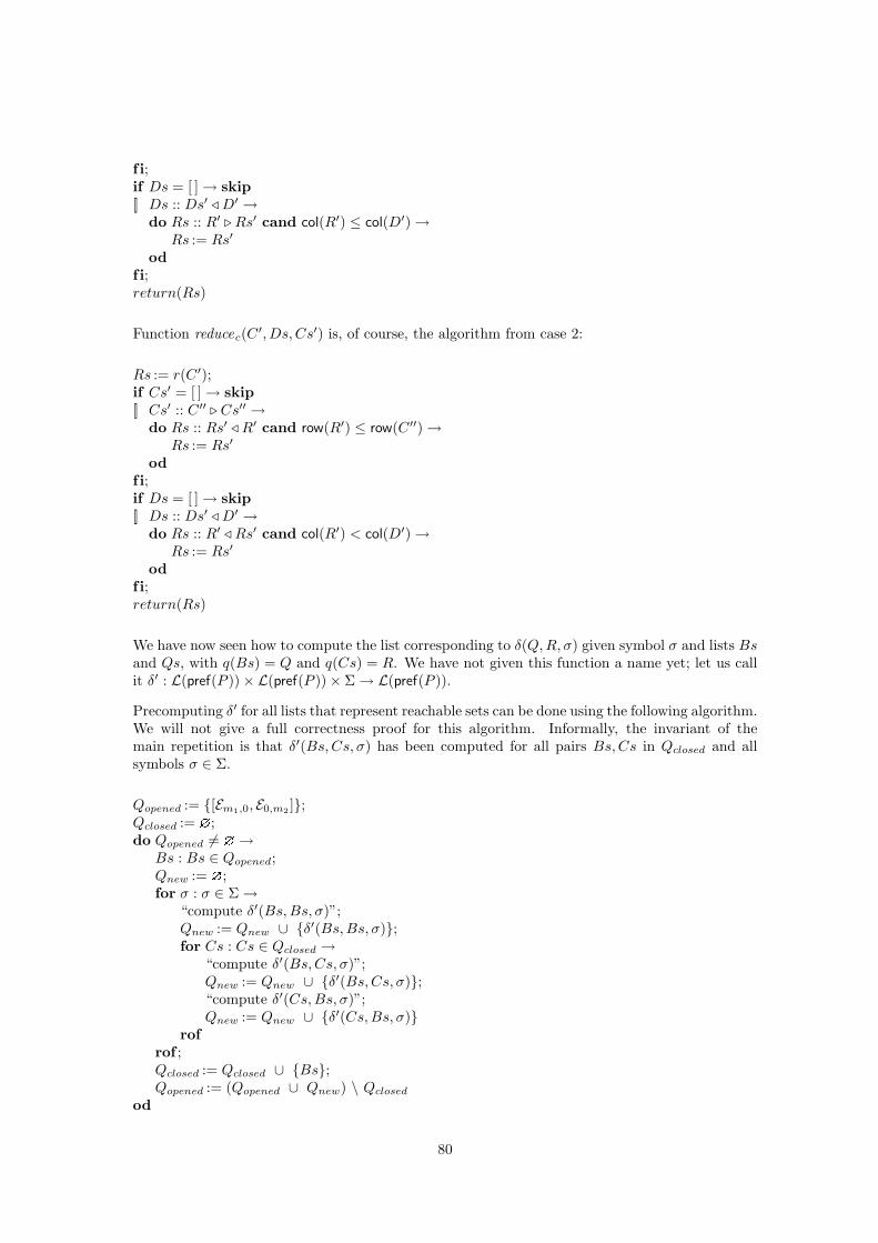
f i;if Ds = [ ] → skip[] Ds :: Ds′ / D′ →

do Rs :: R′ . Rs′ cand col(R′) ≤ col(D′) →Rs := Rs′

odfi;return(Rs)

Function reducec(C ′, Ds, Cs′) is, of course, the algorithm from case 2:

Rs := r(C ′);if Cs′ = [ ] → skip[] Cs′ :: C ′′ . Cs′′ →

do Rs :: Rs′ / R′ cand row(R′) ≤ row(C ′′) →Rs := Rs′

odfi;if Ds = [ ] → skip[] Ds :: Ds′ / D′ →

do Rs :: R′ / Rs′ cand col(R′) < col(D′) →Rs := Rs′

odfi;return(Rs)

We have now seen how to compute the list corresponding to δ(Q, R, σ) given symbol σ and lists Bsand Qs, with q(Bs) = Q and q(Cs) = R. We have not given this function a name yet; let us callit δ′ : L(pref(P ))× L(pref(P ))× Σ → L(pref(P )).

Precomputing δ′ for all lists that represent reachable sets can be done using the following algorithm.We will not give a full correctness proof for this algorithm. Informally, the invariant of themain repetition is that δ′(Bs, Cs, σ) has been computed for all pairs Bs, Cs in Qclosed and allsymbols σ ∈ Σ.

Qopened := {[Em1,0, E0,m2 ]};Qclosed := ?;do Qopened 6= ?→

Bs : Bs ∈ Qopened;Qnew := ?;for σ : σ ∈ Σ →

“compute δ′(Bs,Bs, σ)”;Qnew := Qnew ∪ {δ′(Bs,Bs, σ)};for Cs : Cs ∈ Qclosed →

“compute δ′(Bs, Cs, σ)”;Qnew := Qnew ∪ {δ′(Bs, Cs, σ)};“compute δ′(Cs,Bs, σ)”;Qnew := Qnew ∪ {δ′(Cs,Bs, σ)}

rofrof ;Qclosed := Qclosed ∪ {Bs};Qopened := (Qopened ∪ Qnew) \ Qclosed

od

80

Referring to [IN77, MP04, Pol04] for the definition of tessellation automata, we can say that thiscorresponds to precomputing a two-dimensional deterministic online tessellation automaton withthe following properties:

• alphabet: Σ;

• state set: Qclosed;

• transition function: δ′;

• initial state: [Em1,0, E0,m2 ];

• set of final states: {[P ]}. (Note that suff(P ) ∩ pref(P ) is indeed a reachable set and there-fore [P ] ∈ Qclosed.)

The matrices that occur in the lists in these algorithms are all prefixes of P . If pattern P is known,we can represent a prefix of P uniquely by its size. This means that in an implementation, it isnot necessary to store lists of matrices; lists of integer pairs suffice.

6.3.4 Computation of the “failure function”

As we have seen in section 6.3.2, we still need to find a way to (pre)compute the values of auxiliaryfunction r : pref(P ) → L(pref(P )), specified as follows, for all A ∈ pref(P ):

q(r(A)) = (suff(A) ∩ pref(P )) \ {A}OL(r(A))

First we will consider the cases where A is an empty matrix in isolation.

• row(A) = 0 ∧ col(A) = 0: A = E0,0. Then we can derive:

(suff(E0,0) ∩ pref(P )) \ {E0,0}= { definition suff }

({E0,0} ∩ pref(P )) \ {E0,0}= { set calculus }

?

= { definition q }q([ ])

• row(A) = 0 ∧ 0 < col(A): A = E0,col(A).

(suff(E0,col(A)) ∩ pref(P )) \ {E0,col(A)}= { definition suff, ES }

(ES0,col(A) ∩ pref(P )) \ {E0,col(A)}= { col(A) ≤ m1 }

ES0,col(A) \ {E0,col(A)}= { definition ES, set calculus, 0 < col(A) }

81

ES0,col(A)−1

= { definition pref, ES; col(A) ≤ m1 }ES0,col(A)−1 ∩ pref(P )

= { definition q }q([E0,col(A)−1])

• 0 < row(A) ∧ col(A) = 0. This is completely symmetrical to the previous case and givesus: (suff(A) ∩ pref(P )) \ {A} = q([Erow(A)−1,0]).

The case where A is a nonempty matrix remains. That is, 0 < row(A) ∧ 0 < col(A).

Informally, we want to find a way to compute the list r(A). This list consists of the maximalelements of the set (suff(A)∩pref(P )) \ {A}, ordered by decreasing number of rows and increasingnumber of columns. The method we will describe consists of running a (bounded) linear searchfor each j : 0 ≤ j ≤ row(A), to find the maximal element with exactly j rows, if such a maximalelement exists.

We start with the following observation:

(suff(A) ∩ pref(P )) \ {A}= { property suff, set calculus, 0 < row(A) ∧ 0 < col(A) }

({A} ∩ pref(P )) \ {A} ∪(suff(A[1 .. row(A))[0 .. col(A))) ∩ pref(P )) \ {A} ∪(suff(A[0 .. row(A))[1 .. col(A))) ∩ pref(P )) \ {A}

= { set calculus, definition suff }(suff(A[1 .. row(A))[0 .. col(A))) ∩ pref(P )) ∪

(suff(A[0 .. row(A))[1 .. col(A))) ∩ pref(P ))

= { • introduction of g }g(row(A)− 1) ∪ (suff(A[0 .. row(A))[1 .. col(A))) ∩ pref(P ))

Here we introduce the following auxiliary function:

g(j) = suff(A[row(A)− j .. row(A))[0 .. col(A))) ∩ pref(P )

It may seem that at this point we could simply conclude that A[0 .. row(A))[1 .. col(A)) is the firstelement of r(A). However, we know that r(A) ∈ L(pref(P )) and in general, A[0 .. row(A))[1 .. col(A))does not need to be a prefix of P .

We now introduce variables Rs : L(pref(P )) and i1 : N and the following tail invariant:

P0 : q(r(A)) = q(Rs) ∪ g(i1)

We could initially establish P0 by choosing Rs = [ ] and i1 = row(A). However, it will be useful toconsider the case of i1 = row(A) seperately. Therefore, we choose to initialise i1 = row(A)−1. Theinitialisation of Rs then consists of a repetition; we introduce integer variable i2 and the followingtail invariant:

Q0 : q(r(A)) = g(row(A)− 1) ∪(suff(A[0 .. row(A))[col(A)− i2 .. col(A))) ∩ pref(P ))

82

As we have seen, we can initially choose i2 = col(A) − 1. We can terminate the computationwhen A[0 .. row(A))[col(A) − i2 .. col(A)) = P [0 .. row(A))[0 .. i2), because then the assign-ment Rs := [P [0 .. row(A))[0 .. i2)] establishes P0. We know that a value of i2 exists for whichthis termination condition holds, namely: i2 = 0.

When A[0 .. row(A))[col(A)− i2 .. col(A)) 6= P [0 .. row(A))[0 .. i2), we get:

g(row(A)− 1) ∪ (suff(A[0 .. row(A))[col(A)− i2 .. col(A))) ∩ pref(P ))

= { 0 < row(A), 0 < i2 }g(row(A)− 1) ∪ ({A[0 .. row(A))[col(A)− i2 .. col(A))} ∩ pref(P )) ∪

(suff(A[1 .. row(A))[col(A)− i2 .. col(A))) ∩ pref(P )) ∪(suff(A[0 .. row(A))[col(A)− i2 + 1 .. col(A))) ∩ pref(P ))

= { A[0 .. row(A))[col(A)− i2 .. col(A)) 6= P [0 .. row(A))[0 .. i2) }g(row(A)− 1) ∪ (suff(A[1 .. row(A))[col(A)− i2 .. col(A))) ∩ pref(P )) ∪

(suff(A[0 .. row(A))[col(A)− i2 + 1 .. col(A))) ∩ pref(P ))

= { definition g }g(row(A)− 1) ∪ (suff(A[0 .. row(A))[col(A)− i2 + 1 .. col(A))) ∩ pref(P ))

So the initialisation step of our algorithm now becomes:

i2 := col(A)− 1;{ invariant: Q0 }do A[0 .. row(A))[col(A)− i2 .. col(A)) 6= P [0 .. row(A))[0 .. i2) →

i2 := i2 − 1od;R′ := P [0 .. row(A))[0 .. i2);Rs := [R′];i1 := row(A)− 1{ P0 }

As we can see, we initialise Rs as a list containing one element, R′. This list will only grow in therest of the algorithm text; it will never be an empty list. As an extra invariant we ensure that R′

is always the last element of Rs:

P1 : 〈∃Rs′ : Rs′ ∈ L(pref(P )) : Rs = Rs′ / R′〉

Additionally, we also have as an invariant:

P2 : i1 < row(R′)

Now we can see that we can terminate the computation when col(A) ≤ col(R′):

q(r(A))

= { P0 }q(Rs) ∪ g(i1)

= { definition g }

83

q(Rs) ∪ (suff(A[row(A)− i1 .. row(A))[0 .. col(A))) ∩ pref(P ))

⊆ { col(A) ≤ col(R′) }q(Rs) ∪ (suff(A[row(A)− i1 .. row(A))[col(A)− col(R′) .. col(A))) ∩ pref(P ))

⊆ { P2 }q(Rs) ∪ (suff(A[row(A)− row(R′) .. row(A))[col(A)− col(R′) .. col(A))) ∩ pref(P ))

= { R′ ∈ suff(A) }q(Rs) ∪ (suff(R′) ∩ pref(P ))

= { P1; (8) on page 60 }q(Rs)

Invariant P0 tells us q(Rs) ⊆ q(r(A)), so we have q(Rs) = q(r(A)). And since q(r(A)) is the uniquelist corresponding to r(A) (as we have seen in section 6.3.0), we can then conclude: Rs = r(A).

All that remains is to see how to update Rs and i1. For this we again introduce a repetition, muchlike the one used for initialisation of i1 and Rs, with the following invariant:

R0 : q(r(A)) = q(Rs) ∪ g(i1 − 1) ∪(suff(A[row(A)− i1 .. row(A))[col(A)− i2 .. col(A))) ∩ pref(P ))

Initially we choose i2 = col(A) and, like in the initialisation of i1 and Rs, we can stop thecomputation when we find A[row(A) − i1 .. row(A))[col(A) − i2 .. col(A)) = P [0 .. i1)[0 .. i2).However, we have an additional bound; we should also stop the computation when i2 ≤ col(R′):

q(r(A))

= { R0 }q(Rs) ∪ g(i1 − 1) ∪ (suff(A[row(A)− i1 .. row(A))[col(A)− i2 .. col(A))) ∩ pref(P ))

⊆ { i2 ≤ col(R′) }q(Rs) ∪ g(i1 − 1) ∪ (suff(A[row(A)− i1 .. row(A))[col(A)− col(R′) .. col(A))) ∩ pref(P ))

⊆ { P2 }q(Rs) ∪ g(i1 − 1) ∪ (suff(A[row(A)− row(R′) .. row(A))[col(A)− col(R′) .. col(A))) ∩ pref(P ))

= { R′ ∈ suff(A) }q(Rs) ∪ g(i1 − 1) ∪ (suff(R′) ∩ pref(P ))

= { P1; (8) on page 60 }q(Rs) ∪ g(i1 − 1)

All this gives rise to the following algorithm to compute r(A):

if row(A) = 0 ∧ col(A) = 0 →Rs := [ ]

[] row(A) = 0 ∧ 0 < col(A) →Rs := [E0,col(A)−1]

[] 0 < row(A) ∧ col(A) = 0 →Rs := [Erow(A)−1,0]

[] 0 < row(A) ∧ 0 < col(A) →i2 := col(A)− 1;

84

do A[0 .. row(A))[col(A)− i2 .. col(A)) 6= P [0 .. row(A))[0 .. i2) →i2 := i2 − 1

od;R′ := P [0 .. row(A))[0 .. i2);Rs := [R′];i1 := row(A)− 1;do col(R′) < col(A) →

i2 := col(A);do col(R′) < i2 ∧ A[row(A)− i1 .. row(A))[col(A)− i2 .. col(A)) 6= P [0 .. i1)[0 .. i2) →

i2 := i2 − 1od;if col(r′) < i2 →

R′ := P [0 .. i1)[0 .. i2);Rs := Rs / R′

[] i2 ≤ col(R′) →skip

fi;i1 := i1 + 1

odfi

6.4 Entire algorithm

In section 6.2 we have presented a preliminary version of Polcar’s algorithm, expressed in termsof sets of prefixes of P . To make use of function δ′, precomputed as described in section 6.3, thesesets will need to be represented by the ordered lists of their maximal elements. To replace array e,we introduce array e′ : [0 .. n2] of L(pref(P )), with q(e′[j]) = e[j] and OL(e′[j]) (for 0 ≤ j ≤ n2).Furthermore, we note:

P ∈ q(e′[j])

≡ { OL(e′[j]); e′ ∈ L(pref(P )) }e′[j] = [P ]

We get the following algorithm:

O := ?;for j : 0 ≤ j ≤ n2 → e′[j] := [Em1,0, E0,m2 ] rof ;i1, i2 := 0, 0;do i1 6= n1 →

do i2 6= n2 →e′[i2 + 1] := δ′(e′[i2 + 1], e′[i2], T [i1, i2]);if e′[i2 + 1] = [P ] → O := O ∪ {(i1 + 1−m1, i2 + 1−m2)}[] e′[i2 + 1] 6= [P ] → skipfi;i2 := i2 + 1

od;i2 := 0;i1 := i1 + 1

od

85

6.5 Remarks

There are a few differences between this version of the algorithm and the original presentations in[Pol04, MP04].

In the original presentations, a so-called (nondeterministic) two-dimensional online tessellationautomaton (2OTA) is constructed, where each state in the 2OTA corresponds to a prefix ofthe pattern. This 2OTA is transformed into a two-dimensional deterministic online tessellationautomaton (2DOTA), using an algorithm very similar to the subset construction.3 As a result,the states in the resulting 2DOTA (implicitly) each correspond to a set of prefixes of P .

In our presentation, we do not need to introduce tessellation automata. Nor do we first constructan equivalent of the 2OTA; we immediately derive an algorithm to precompute the values of δ′,which is the equivalent of the 2DOTA’s transition function.

As we have seen in section 6.3.0, we do start out our derivation of the “transition function” δ′ byexamining sets of prefixes of P , but we represent these sets by a list of their maximal elements. Thisapproach improves the precomputation’s performance and is more similar to the one-dimensionalpattern matching algorithms which Polcar’s algorithm is based on: Aho-Corasick and Knuth-Morris-Pratt ([AC75, KMP77]).

Even with these improvements, the precomputation for this algorithm can be very unefficient.However, the precomputation’s performance depends only on the size of the pattern. As a result,Polcar’s algorithm is most useful when the pattern is relatively very small, compared to the text.

3The subset construction is an algorithm used for transforming a (one-dimensional) nondeterministic finiteautomaton (NFA) into a deterministic finite automaton (DFA). See [ASU96], pages 117–121.

86

87

7 Conclusions and future work

7.0 Conclusions

We have described several, very different, two-dimensional pattern matching algorithms. Some arevery well-known, such as the Baker-Bird algorithm ([Bak78, Bir77]), the first known solution tothe problem. On the other hand we have also described the very recent Polcar algorithm ([Pol04,MP04]), which was first presented in 2004.

All of these algorithms have been formally derived. The derivations are formal proofs that thesealgorithms are correct solutions to the two-dimensional pattern matching problem, while theirpresentations in existing literature usually lack such full correctness proofs. The derivations alsoshow where we have taken some of the major design decisions, such as the choice of a filter functionin the filter-based algorithms (see section 4.0 on page 20). This can be very useful in discoveringnew two-dimensional pattern matching algorithms.

We have described the similarities between the Baker-Bird and Takaoka-Zhu ([TZ89, TZ94]) al-gorithms, by presenting both using a uniform description, as so-called filter-based algorithms.Because of this it became immediately obvious that a space complexity improvement, first sug-gested in the original presentation of Takaoka-Zhu, was also applicable to the Baker-Bird algorithm(and almost any other possible filter-based algorithm; see section 4.2 on page 22).

We have derived Baeza-Yates and Regnier’s algorithm ([BYR93]) and also proposed two improve-ments over its original presentation (section 5.2 on page 36 and section 5.3 on page 39). Both ofthese improvements use information obtained during a failed matching attempt to speed up thecomputation by skipping unnecessary row comparisons.

Polcar’s algorithm was derived without using the tessellation automata data structure or any ofits properties. In addition, we have shown an improvement in the precomputation step of thisalgorithm: where Polcar’s approach uses sets of matrices, we have represented these sets by listsof the maximal elements of these sets (see section 6.3 on page 56). This is an improvement ofboth the time and space complexity of the precomputation. It is also an interesting improvementbecause it is so similar to the approach of the one-dimensional Aho-Corasick and Knuth-Morris-Pratt algorithms ([AC75, KMP77]): there too we reason in terms of strings of maximal length, asopposed to sets of strings (see also [WZ92, WZ93]).

Part of the original goal of this research was to create a taxonomy of two-dimensional patternmatching algorithms. We have not done this yet, because the algorithms we have seen differ greatlyfrom each other, with the exception of the filter-based algorithms: Baker-Bird and Takaoka-Zhu.Given these great differences a taxonomy would only have a very course structure, not giving anyadditional information or insight.

7.1 Future work

Although we have derived several two-dimensional pattern matching algorithms, there are stillknown algorithms that have not been described in this thesis. Future research can include thederivation of more known algorithms. Also, there may be many solutions to the two-dimensionalpattern matching problem that have not been discovered yet. In particular, exploring other choicesfor the filter function in the filter-based approach (see section 4 on page 20) may lead to newsolutions. When more algorithms have been derived, constructing a taxonomy will be useful.

Existing pattern matching toolkits, such as SPARE Time and SPARE Parts (see [Cle03]), canbe expanded to include the two-dimensional pattern matching algorithms described in this thesis.

88

However, matrices are a rather different data structure than strings, so generalising existing toolkitsto include two-dimensional pattern matching strategies may be difficult; in that case, a seperatetoolkit for two-dimensional pattern matching can be developed, in the same style as SPARE Timeand SPARE Parts.

Once an efficient and practical implementation has been constructed, it is possible to perform abenchmarking; that is, a thorough practical performance analysis. A complete theoretical per-formance analysis (of memory and time complexity) can be done for the algorithms describedhere as well. We can refer to the original presentations of the algorithms for their space andtime complexity; however, it is unknown how the improvements made to the Baeza-Yates andRegnier algorithm and the Polcar precomputation algorithm affect their average-case theoreticalperformance exactly.

Further generalisations of the two-dimensional pattern matching problem are also possible andworth exploring. We have already briefly discussed generalisation to multipattern matching andmatching in more than two dimensions for most algorithms. Other generalisations include approx-imate two-dimensional pattern matching (where we need to define a distance function in terms ofmatrices) and matching patterns of non-rectangular shapes. (This last generalisation can be solvedusing the algorithms presented here, by introducing a “don’t care” symbol, which matches withevery symbol of the text, and expanding the pattern to a bounding rectangle with this symbol.However, more efficient solutions may be possible.)

89

A Properties of div and mod

Definition A.0 For a ∈ N and q ∈ N+ we define div and mod by:

a = (a div q) ∗ q + a mod q0 ≤ a mod q < q

Theorem A.1 For all a, b ∈ N and q ∈ N+ we have:

(a ∗ q + b) mod q = b mod q

Proof

(a ∗ q + b) mod q

= { def. div and mod : b = (b div q) ∗ q + b mod q }(a ∗ q + (b div q) ∗ q + b mod q) mod q

= { ∗ over + }((a + b div q) ∗ q + b mod q) mod q

= { 0 ≤ b mod q < q; def. div and mod : X = Y ∗ q + Z ∧ 0 ≤ Z < q ⇒ Z = X mod q }b mod q

�

Theorem A.2 For all a, b, c ∈ N and q ∈ N+ we have:

(a ∗ b + c) mod q = ((a mod q) ∗ b + c) mod q

Proof

(a ∗ b + c) mod q

= { a = (a div q) ∗ q + a mod q }(((a div q) ∗ q + a mod q) ∗ b + c) mod q

= { ∗ over + }((a div q) ∗ q ∗ b + (a mod q) ∗ b + c) mod q

= { theorem A.1 }((a mod q) ∗ b + c) mod q

�

Theorem A.3 For a ∈ N and q ∈ N+:

a ≤ (a div q + 1) ∗ q − 1 < a + q

90

Proof

First we note:

(a div q + 1) ∗ q − 1 = (a div q) ∗ q + q − 1

Now we can prove the theorem with the following derivation:

a

= { definition div and mod }(a div q) ∗ q + a mod q

≤ { a mod q < q }(a div q) ∗ q + q − 1

≤ { 0 ≤ a mod q }(a div q) ∗ q + a mod q + q − 1

= { definition div and mod }a + q − 1

< { math }a + q

�

91

B Properties of pref and suff (for strings)

Theorem B.0 For x, y ∈ Σ∗:

suff(xy) = suff(x)y ∪ suff(y)

Proof In the following derivation, bound variables v and w are both strings over Σ. We willomit v, w ∈ Σ∗ in our set quantifications.

suff(x)y ∪ suff(y)

= { suff, twice }〈set v, w : vw = x : w〉y ∪ 〈set v, w : vw = y : w〉

= { concatenation over set }〈set v, w : vw = x : wy〉 ∪ 〈set v, w : vw = y : w〉

= { dummy transformation, twice }〈set v, w : |y| ≤ |w| ∧ vw = xy : w〉 ∪ 〈set v, w : |w| ≤ |y| ∧ vw = xy : w〉

= { set calculus (note overlap of |w| = |y|) }〈set v, w : vw = xy : w〉

= { suff }suff(xy)

�

Theorem B.1 For x, y ∈ Σ∗ and a ∈ Σ:

suff(xay) = suff(x)ay ∪ suff(y)

Proof

suff(xay)

= { theorem B.0 }suff(xa)y ∪ suff(y)

= { property suff }suff(x)ay ∪ {y} ∪ suff(y)

= { y ∈ suff(y) }suff(x)ay ∪ suff(y)

�

92

93

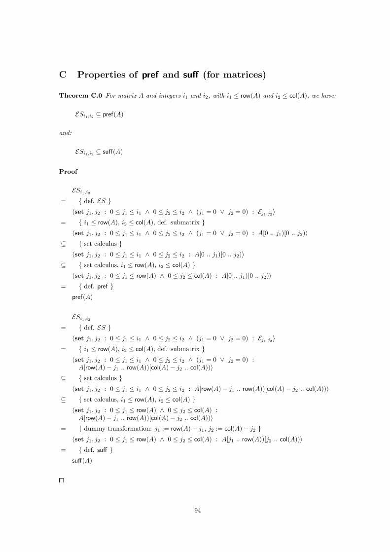
C Properties of pref and suff (for matrices)

Theorem C.0 For matrix A and integers i1 and i2, with i1 ≤ row(A) and i2 ≤ col(A), we have:

ESi1,i2 ⊆ pref(A)

and:

ESi1,i2 ⊆ suff(A)

Proof

ESi1,i2

= { def. ES }〈set j1, j2 : 0 ≤ j1 ≤ i1 ∧ 0 ≤ j2 ≤ i2 ∧ (j1 = 0 ∨ j2 = 0) : Ej1,j2〉

= { i1 ≤ row(A), i2 ≤ col(A), def. submatrix }〈set j1, j2 : 0 ≤ j1 ≤ i1 ∧ 0 ≤ j2 ≤ i2 ∧ (j1 = 0 ∨ j2 = 0) : A[0 .. j1)[0 .. j2)〉

⊆ { set calculus }〈set j1, j2 : 0 ≤ j1 ≤ i1 ∧ 0 ≤ j2 ≤ i2 : A[0 .. j1)[0 .. j2)〉

⊆ { set calculus, i1 ≤ row(A), i2 ≤ col(A) }〈set j1, j2 : 0 ≤ j1 ≤ row(A) ∧ 0 ≤ j2 ≤ col(A) : A[0 .. j1)[0 .. j2)〉

= { def. pref }pref(A)

ESi1,i2

= { def. ES }〈set j1, j2 : 0 ≤ j1 ≤ i1 ∧ 0 ≤ j2 ≤ i2 ∧ (j1 = 0 ∨ j2 = 0) : Ej1,j2〉

= { i1 ≤ row(A), i2 ≤ col(A), def. submatrix }〈set j1, j2 : 0 ≤ j1 ≤ i1 ∧ 0 ≤ j2 ≤ i2 ∧ (j1 = 0 ∨ j2 = 0) :

A[row(A)− j1 .. row(A))[col(A)− j2 .. col(A))〉⊆ { set calculus }

〈set j1, j2 : 0 ≤ j1 ≤ i1 ∧ 0 ≤ j2 ≤ i2 : A[row(A)− j1 .. row(A))[col(A)− j2 .. col(A))〉⊆ { set calculus, i1 ≤ row(A), i2 ≤ col(A) }

〈set j1, j2 : 0 ≤ j1 ≤ row(A) ∧ 0 ≤ j2 ≤ col(A) :A[row(A)− j1 .. row(A))[col(A)− j2 .. col(A))〉

= { dummy transformation: j1 := row(A)− j1, j2 := col(A)− j2 }〈set j1, j2 : 0 ≤ j1 ≤ row(A) ∧ 0 ≤ j2 ≤ col(A) : A[j1 .. row(A))[j2 .. col(A))〉

= { def. suff }suff(A)

�

94

Theorem C.1 For all A ∈M2(Σ) and k1, k2 ∈ N:

ESk1,k2 ∩ pref(A) = ESk1↓row(A),k2↓col(A)

Proof

ESk1,k2 ∩ pref(A)

= { def. ES, def. pref }(〈set j : 0 ≤ j ≤ k1 : Ej,0〉 ∪ 〈set j : 0 ≤ j ≤ k2 : E0,j〉) ∩〈set i1, i2 : 0 ≤ i1 ≤ row(A) ∧ 0 ≤ i2 ≤ col(A) : A[0 .. i1)[0 .. i2)〉

= { ∩ over ∪, set calculus }〈set j, i1, i2 : 0 ≤ j ≤ k1 ∧ 0 ≤ i1 ≤ row(A) ∧ 0 ≤ i2 ≤ col(A) ∧ A[0 .. i1)[0 .. i2) = Ej,0 : Ej,0〉 ∪〈set j, i1, i2 : 0 ≤ j ≤ k2 ∧ 0 ≤ i1 ≤ row(A) ∧ 0 ≤ i2 ≤ col(A) ∧ A[0 .. i1)[0 .. i2) = E0,j : E0,j〉

= { def. submatrix, math }〈set j : 0 ≤ j ≤ k1 ↓ row(A) : Ej,0〉 ∪ 〈set j : 0 ≤ j ≤ k2 ↓ col(A) : E0,j〉

= { def. ES }ESk1↓row(A),k2↓col(A)

�

95

D Lists

Here we will briefly describe the notation we use for lists.

• [ ]: the empty list.

• As ++ Bs: the concatenation of lists As and Bs.

• A . As: the list which consists of element A, followed by As; equivalently: [A] ++ As. Inother terminology, A is the head of the list and As the tail.

• As / A: the list which consists of As, followed by element A; equivalently: As ++ [A].

96

97

References

[AC75] Alfred V. Aho and Margaret J. Corasick. Efficient string matching: an aid to biblio-graphic search. Communications of the ACM, 18(6):333–340, June 1975.

[ASU96] Alfred V. Aho, Ravi Sethi, and Jeffrey D. Ullman. Compilers: principles, techniquesand tools. Addison-Wesley, 1996.

[Bak78] Theodore P. Baker. A technique for extending rapid exact-match string matching toarrays of more than one dimension. SIAM Journal on Computing, 7(4):533–541, 1978.

[Bir77] Richard Bird. Two dimensional pattern matching. Information Processing Letters,6(5):168–170, 1977.

[BYR93] Ricardo Baeza-Yates and Mireille Regnier. Fast two-dimensional pattern matching.Information Processing Letters, 45(1):51–57, 1993.

[Cle03] Loek Cleophas. Towards SPARE Time. Master’s thesis, Technische Universiteit Eind-hoven, August 2003.

[CR02] Maxime Crochemore and Wojciech Rytter. Jewels of stringology. World Scientific, 2002.

[IN77] Katsushi Inoue and Akira Nakamura. Some properties of two-dimensional online tessel-lation acceptors. Information sciences, 43:169–184, 1977.

[KMP77] Donald E. Knuth, James H. Morris, and Vaughan R. Pratt. Fast pattern matching instrings. SIAM Journal of Computing, 6(2):323–350, 1977.

[KR87] Richard M. Karp and Michael O. Rabin. Efficient randomized pattern-matching algo-rithms. IBM Journal of Research and Development, 31(2):249–260, March 1987.

[MP04] Borivoj Melichar and Tomas Polcar. A two-dimensional online tessellation automataapproach to two-dimensional pattern matching. In Loek Cleophas and Bruce W. Watson,editors, Proceedings of the Eindhoven FASTAR days 2004. Computer science report04/40, Technische Universiteit Eindhoven, December 2004.

[MZ05] Borivoj Melichar and Jan Zd’arek. On two-dimensional pattern matching by finiteautomata. In J. Farre, I. Litovsky, and S. Schmitz, editors, CIAA 2005 pre-proceedings,pages 185–194, 2005.

[NR02] Gonzalo Navarro and Mathieu Raffinot. Flexible pattern matching in strings. CambridgeUniversity Press, 2002.

[Pol04] Tomas Polcar. Two-dimensional pattern matching. Postgraduate study report DC-PSR-04-05, Czech Technical University, January 2004.

[RS97] G. Rozenberg and A. Salomaa. Handbook of formal languages, volume 3: Beyond words,chapter 4: Two-dimensional languages, pages 215–267. Springer-Verlag, Berlin, 1997.

[TZ89] Tadao Takaoka and Rui Feng Zhu. A technique for two-dimensional pattern matching.Communications of the ACM, 32(9):1110–1120, 1989.

[TZ94] Tadao Takaoka and Rui Feng Zhu. A technique for two-dimensional pattern matching. InJun-Ichi Aoe, editor, String pattern matching strategies, pages 220–230. IEEE ComputerSociety Press, 1994.

[Wat95] Bruce W. Watson. Taxonomies and toolkits of regular language algorithms. PhD thesis,Technische Universiteit Eindhoven, 1995.

98

[WZ92] Bruce W. Watson and Gerard Zwaan. A taxonomy of keyword pattern matching algo-rithms. Computing science report 92/27, Technische Universiteit Eindhoven, 1992.

[WZ93] Bruce W. Watson and Gerard Zwaan. A taxonomy of keyword pattern matching algo-rithms. In H. A. Wijshoff, editor, Proceedings Computing Science in the Netherlands93, pages 25–39, SION, Stichting Mathematish Centrum, 1993.

[WZ95] Bruce W. Watson and Gerard Zwaan. A taxonomy of sublinear keyword pattern match-ing algorithms. Computing science report 95/13, Technische Universiteit Eindhoven,1995.

[WZ96] Bruce W. Watson and Gerard Zwaan. A taxonomy of sublinear multiple keyword pat-tern matching algorithms. Science of Computer Programming, 27(2):85–118, September1996.

99