Embed Size (px)
Citation preview

1
Pushing and Pulling: Determinants of migration during Sweden's industrialisation
Björn Eriksson
Centre for Economic Demography, Department of Economic History, Lund University
Siddartha Aradhya
Stockholm University Demography Unit, Department of Sociology, Stockholm University
Finn Hedefalk
Centre for Economic Demography, Department of Economic History, Lund University
Please note that this is a preliminary draft. In the final version, we will also consider
emigration to the US as part of the emigration decision.

2
Introduction
Ravenstein’s (1885, 1889) “The Laws of Migration” laid the foundation of the push and pull
model of migration which has provided the basic framework for analysing migration for more
than a century. Its simple intuition stands in contrast to the empirical challenges associated
with estimating the parameters of the model. In his seminal work, Ravenstein used late
nineteenth century censuses to generalize the predominant causes of migration. In this spirit
we take a fresh look at the historical determinants of migration using linked historical census
data.
There is a rich historical literature which considers the impact of economic conditions and
individual characteristics on migration and destination choice using either aggregate or micro
data.. Examples include studies of nineteenth century European circular and rural to urban
migration (Söderberg 1985; Boyer 1997; Boyer and Hatton 1997; Lundh 1999; Dribe 2003;
Grant 2005; Long 2005; Silvestre 2005) the trans-Atlantic emigration from Europe to North
America (Gallaway and Vedder 1971; Hatton 1997; Hatton and Williamson 1998; Bohlin and
Eurenius 2010; Abramitzky, Platt Boustan and Eriksson 2013) and the labour migration from
the rural American South to the industrialised North (Collins and Wanamaker 2014, 2015;
Hornbeck and Naidu 2014; Black et al. 2015). Aggregate analysis typically relies on some
form of gravity model to estimate push and pull parameters based on migration flows. Micro
data allows for the explicit modelling of either the migration decision or the choice of
destination using discrete choice analysis. Both approaches have its shortcomings: aggregate
analysis prohibits conclusions to be drawn regarding individual behaviour while micro data
tends to be constrained geographically and limited to migrations between a subset of possible
origins and destinations.
This paper seeks to improve on past studies through the use of new data and a more
comprehensive empirical migration model. We contribute to the literature by modelling the
complete migration decision at the individual level, considering both the decision between
staying and migrating and the subsequent destination choice.1 Our methodological approach
facilitates simultaneous modelling of the migration decision and the destination choice, also
1 Because of data limitations, emigration, which primarily took place to the US, has been omitted from the analysis.
3
accounting for individual characteristics. We are thus able to estimate push and pull factors as
part of one individual utility maximizing decision, and not separately as normally done.
Our focus is on late nineteenth century Sweden, a country experiencing rapid economic
growth and increasing rates of internal migration. The analysis is based on a cohort of men
and women born between 1860 and 1870 that transitioned into adulthood during the height of
Swedish industrialisation. These men and women are first observed as adolescents residing
with their parents in 1880, and then again ten years later in 1890. Upon leaving their parental
home, most moved a relatively short distance, often to a rural area not dissimilar to that in
which they were born. By doing so, these migrants were following a well-established pattern
dating back to pre-industrial Sweden. Many did however not follow in these well-trodden
tracks, instead migrating further away. We focus on these medium and long range moves by
considering inter county migration and the push and pull factors which determined the
migration decision and the location choice.
Push and pull factors
Ravenstein’s (1885) “The Laws of Migration” laid the foundation upon which the early push
and pull factors of migration were developed. In this seminal work, Ravenstein used the 1871
and 1881 censuses from the United Kingdom to generalize the predominant drivers of
migration. The main conclusions from his analysis were that individuals migrate to improve
their economic prospects, a finding reiterated by Hicks (1932:75) who argued that
“…differences in net economic advantages, chiefly differences in wages, are the main cause
of migration”.
From an individual perspective migration may be conceptualised as an investment decision in
which each possible move is associated with certain costs and benefits. Expectations about
the benefits of migrating to a certain locations are formed based on anticipated income gains
and other non-pecuniary amenities.If the net return from moving is positive, migration
subsequently takes place to the chosen destination (Sjastaad 1962). Several aspects relating to
individual characteristics, the origin, potential destinations and intervening factors all form
part of the decision process and affect the probability of migration and the destination choice
(Lee 1966; Borjas 1987). This study is grounded in this framework through the explicit
4
modelling of push and pull factors at both the macro and micro level. In doing so, one must
consider the economic drivers of migration, the intervening obstacles, and the individual
characteristics of the migrants.
Economic conditions
Important migration flows are typically analysed and understood as the result of economic
differences between sending and receiving regions. Within this paradigm, individuals from
regions with a large endowment of labour relative to capital migrate to destinations with
higher wages and lower relative endowments of labour in order to improve their economic
conditions, a process which proceeds until an equilibrium state between the source and
destination is met (Barro and Sala-i-Martin 1991). Consequently, when modelling the
migration decision, the economic characteristics at both the origin and possible destinations
are important in order to accurately assess the push and pull mechanisms at play. Historically,
economic differences has been shown to be an important explanation for migration from
mainly agricultural and rural areas, with plentiful labour and low wages, to urban and
industrialized areas where labour was in demand and wages accordingly higher (Bengtsson
1990; Boyer 1997; Boyer and Hatton 1997; Silvestre 2005; Grant 2000). As a consequence
migration eroded geographic differences and drove wages to convergence both between and
within countries (Boyer and Hatton 1997; Taylor and Williamson 1997). In Sweden,
aggregate migration flows were an important factor in driving regional convergence,
particularly in the period leading up to 1910 (Enflo, Lundh and Prado 2014; Enflo and Roses
2015).
At the micro-level, migration decisions are conducted at the individual level through a cost
benefit analysis of expected returns to migration. Therefore, regional wage differentials may
not systematically drive migration, as skilled and unskilled migrants are driven by separate
economic influences. Differences in earnings and skill premiums may thus reflect distinct
occupational structure and returns to skills between the destination and origin (Borjas 1987).
By moving to a location with better prospects for upward occupational mobility, anticipated
earnings increase as a result (Sjaastad 1962; Long 2005; Borjas 1989). Moreover, these
expectations should be adjusted in order to account for differences in the probability of

5
employment (Harris and Todaro 1970). The unemployment characteristics of the destination
region may thus play an important role in determining migration (Todaro 1969, 1970)2.
Intervening factors
Distance is one of the most consistently observed determinants of destination choice, with
more remote locations being consistently less attractive destinations than those nearby. (see
Thomas 1938:420-21; Schwartz 1973; ) Ravenstein (1885: 199) noted that ‘migrants
enumerated in a certain centre of absorption will consequently grow less with the distance
proportionately to the native population which furnishes them.'
In terms of costs, the distance between two locations is a proxy for both upfront monetary
costs associated with a particular move, and the psychological cost implied by the separation
from amenities in the origin such as friends and family (Sjaastad 1962; Schwartz 1973).
Apart from affecting the cost side of the migration decision, distance also captures
differences in the information available about a given location. With distance, the uncertainty
about conditions in a location thus increases, making migration to more remote places riskier
(Greenwood 1975). More remote locations are also less likely choices because of what
Stouffer (1940; 1960) termed “intervening opportunities”: with increasing distance, the
number of competing destinations increase, making distant locations less likely to be chosen.
Regional and individual characteristics may serve to mediate the effect of distance. At the
regional level, access to transportation and communication infrastructure such as roads,
railways and postal services serves to lower the cost associated with distances between
locations (Killick 2013). Networks, defined as a community of family and friends (kinship
networks), or migrants from the same origin (migrant network), can help to decrease the costs
associated with migrating. In particular, psychological, information, job-search, and housing
costs will be lower for individuals with large networks, as previously settled migrants can
help more recent ones navigate life in the destination (Yap 1977; Hugo 1981; Taylor 1986;
Massey and Garcia Espana 1987). As Carrington et al. (1996) points out, however, if
networks reduce the costs associated with migration, migration costs will be endogenous to
2 These expectations should be adjusted in order to account for differences in the probability of employment (Harris and Todaro
1970) we have yet to find an indicator of regional unemployment differences.
6
the volume of previous migrations to a given destination. Nonetheless, networks have
received extensive theoretical and empirical support in the literature (Bodvarsson et al 2014).
Individual characteristics
Expectations, ability, benefits, costs and resources are all characteristics that vary between
individuals and simultaneously determine the incidence of migration and the return thereof.
Migration is as a result a highly endogenous process undertaken by a certain groups and
individuals, each differently selected depending on individual characteristics and
circumstances. If costs are important, the expectation is selection of the most able, ambitious
and entrepreneurial part of the population who are able to recoup costs in the form of
substantial returns (Lee 1966). Similarly, costs may affect selection if cost is a negative
function of ability, the able being, in Chiswick’s (1999) words “more efficient in migration”.
Upfront migration costs may also serve as a more direct barrier by preventing the financially
constrained from moving. Even when costs are fixed, as in the case of a train or boat ticket,
migration is still relatively more expensive for the less able because fewer hours of work are
required on the part of the more able to cover expenses associated with a move. Selection
may also be negative if there are regional differences in terms of returns to skills which will
result in opposing migrant streams of skilled and unskilled persons drawn to locations in
which the returns to skills are consummate with individual ability (Roy 1951; Borjas 1987).
Although migrants tend to be younger, the relationship between age and the probability of
migrating is less straightforward. Becker (1964) argues that the propensity to migrate
decreases with age, because the net present value of benefits is higher from younger
prospective migrants due to greater duration of stay in a particular destination. Older workers
may also be less mobile the costs of liquidating physical and personal investments in the
origin is higher (Gallaway 1969; Schwartz 1976; Lundborg 1991). Note, however, that
migration costs may be more affordable for older prospective migrants than younger ones due
to higher earnings and accumulated assets.
Swedish industrialisation and migration
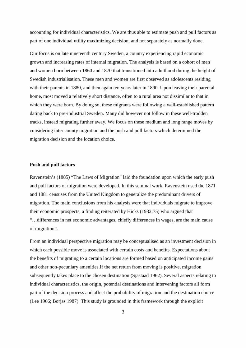
In step with Sweden’s industrial take off, migration increased in response to higher wages in
industrialising regions (The Institute for Social Sciences 1941:42; Jörberg 1972: 348). As can
be seen in Figure 1, only 7% of the population in 1860 resided in a county different from
their county of birth; by 1900 however, the share of county migrants had more than doubled
7
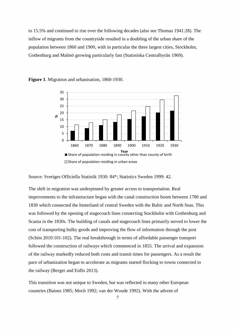
to 15.5% and continued to rise over the following decades (also see Thomas 1941:28). The
inflow of migrants from the countryside resulted in a doubling of the urban share of the
population between 1860 and 1900, with in particular the three largest cities, Stockholm,
Gothenburg and Malmö growing particularly fast (Statistiska Centralbyrån 1969).
Figure 1. Migration and urbanisation, 1860-1930.
Source: Sveriges Officiella Statistik 1930: 84*; Statistics Sweden 1999: 42.
The shift in migration was underpinned by greater access to transportation. Real
improvements to the infrastructure began with the canal construction boom between 1780 and
1830 which connected the hinterland of central Sweden with the Baltic and North Seas. This
was followed by the opening of stagecoach lines connecting Stockholm with Gothenburg and
Scania in the 1830s. The building of canals and stagecoach lines primarily served to lower the
cost of transporting bulky goods and improving the flow of information through the post
(Schön 2010:101-102). The real breakthrough in terms of affordable passenger transport
followed the construction of railways which commenced in 1855. The arrival and expansion
of the railway markedly reduced both costs and transit times for passengers. As a result the
pace of urbanization began to accelerate as migrants started flocking to towns connected to
the railway (Berger and Enflo 2013).
This transition was not unique to Sweden, but was reflected in many other European
countries (Baines 1985; Moch 1992; van der Woude 1992). With the advent of
0
5
10
15
20
25
30
35
1860 1870 1880 1890 1900 1910 1920 1930
%
YearShare of population residing in county other than county of birth
Share of population residing in urban areas
8
industrialisation the population of Europe had entered a new phase of geographic mobility.
As a result of falling transportation costs, a declining agricultural sector and new
opportunities outside of farming, the nature of migration was changing. Instead of making a
living in agriculture, increasing numbers of people were leaving the countryside in favour of
cities.
The shift towards longer distance migration does however not mean that pre-industrial
Sweden was geographically immobile. Rural Swedish societies were in fact characterised by
high rates of geographic mobility (Gaunt 1977:195, Dribe 2000:5-6, Dribe 2003). Migration
was to a large extent driven by frequent short distance moves between rural areas by young
people working as servants (Eriksson and Rogers 1978; Dribe & Lundh 2005). Migration was
tied to the seasons and was the means by which the young earned their keep and acquired
skills in agricultural work (Moch 1992: 61).
As long as certain administrative requirements were met there were no legal obstacles to
internal migration in Sweden during the nineteenth century. Before moving, a prospective
migrant was required to notify the ministers of both the home and destination parish.
Permission to settle in a new parish was given as long as it was not suspected that the migrant
would have difficulty supporting him- or herself. Refusal of permission to move was
exceedingly rare, with less than 1 per cent of applications denied (Eriksson & Rogers
1978:180-181). One institutional barrier to migration did however exist, the Servants Act,
which in particular hampered migration for agricultural workers. The act mandated that
yearly employment contracts for farmhands and maids must begin on the 1st of November
and run until the 24th of October the following year. This resulted in little down time between
employment contracts, which made it difficult for farm workers to find employment
anywhere beyond the vicinity of their last place of work (Lundh 1999:61; Lundh 2003).
Data and descriptive statistics
This paper combines individual panel data and contextual level data in order to model the
migration decision in a comprehensive manner. The individual level data comes from the
complete Swedish censuses of 1880 and 1890. The contextual level data is drawn from
historical official statistics and constructed regional wage and GDP series.
9
Linked census data
The censuses are the most comprehensive source of individual level data for Sweden around
the turn of the century. The Swedish censuses differ from the U.S. and British censuses by
not being the product of a census taking done by enumerators actually visiting and counting
the populace. Instead, with one exception, that of the city of Stockholm, the Swedish
censuses were the result of a compilation of excerpts from continuous parish registers which
were kept by the Swedish Lutheran church and maintained by the parish priest. For
Stockholm, the source of the census were excerpts from the Roteman register, an
administrative register supervised by Mantalsnämnden (The population and tax registration
board), which replaced the Church registers in 1878 in order to cope with the rapidly
growing, and increasingly mobile, population of Stockholm at the end of the nineteenth
century (Geschwind & Fogelvik 2000:207-208).
Because the Swedish census is no more than an excerpt from a continuous and consistent
source rather than a recreation of a population register as in the case of the U.S. and British
censuses, the quality of the raw data is comparatively better. Any errors resulting from the
misreporting by the enumerated or recording mistakes by enumerators may thus be largely
discounted. Moreover, because Swedes were entered into the parish books at the time of
christening and not removed until time of death or emigration, the under-enumeration of the
population as whole and specific groups is less of a problem than what is normally expected
from historical censuses.
The analysis relies on a new panel sample which has been created by linking individuals
between the 1890 and 1880 Swedish complete count censuses. The linking process relies on
exact comparisons of sex, birth place and birth year, and probabilistic matching of names for
identifying and linking individuals between the censuses. Importantly, and uniquely, women
appear with their maiden name, even after marriage, in the Swedish censuses. This enabled
women to be linked to nearly the same extent as men between the two censuses. For a
thorough discussion of the linking process see Eriksson (2015; 2016)
From the linked sample a sub-sample of men and women that were born between 1860 and
1870 were selected. We further restrict the analytical sample to those that resided with their
father in 1880 in order to collect information about social status. One significant group has by
necessity been excluded from the analysis: emigrants. The reason is that in order to be linked
10
between the censuses, an individual had to reside in Sweden in both 1880 and 1890. Anyone
emigrating out of Sweden between the two time points was thus lost in the linking process.
After restricting our sample according to the above criteria, we are left with 308,397
individuals evenly distributed by sex.
We include a number of individual characteristics theorised to affect migration. We use
HISCO coded occupations and the HISCLASSS scheme to classify the social status of an
individual’s father into one of four categories; white collar (HISCLASS 1-5), farmer
(HISCLASS 8 with a HISCO code that corresponds to the occupation of farmer), skilled and
low skilled (HISCLASS 6-10) and unskilled (HISCLASS 11-12) (see van Leeuwen et al.
2002 and van Leeuwen et al. 2011). To account for the effect of previous migration
experiences we coded any individual residing in a county in 1880 which was different from
his or her county of birth as a previous migrant. The migrant status of an individual’s mother
or father was coded in the same manner. The definition of whether an individual was an
urban resident in 1880 follows the definition from the 1880 census. Access to transportation
infrastructure is measured by calculating the distance from each individual’s parish of
residence to the nearest railway in 1880 (The extent of the railway network comes from
BISOS L 1881). In order to account for access to sea transport, the distance to the nearest
coast was calculated in the same way as for railways. Finally, we calculated the distance from
the parish of residence to the county border in order to control for the fact that individuals
located closer to a county border are mechanically more prone to be defined as migrants. We
use the log of all distances when estimating our models.
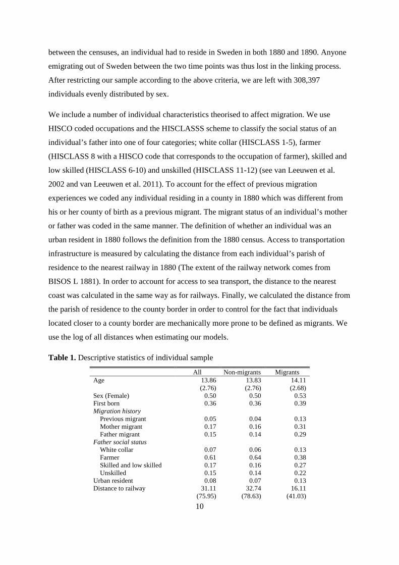
Table 1. Descriptive statistics of individual sample
All Non-migrants Migrants Age 13.86 13.83 14.11 (2.76) (2.76) (2.68) Sex (Female) 0.50 0.50 0.53 First born 0.36 0.36 0.39 Migration history
Previous migrant 0.05 0.04 0.13 Mother migrant 0.17 0.16 0.31 Father migrant 0.15 0.14 0.29
Father social status White collar 0.07 0.06 0.13 Farmer 0.61 0.64 0.38 Skilled and low skilled 0.17 0.16 0.27 Unskilled 0.15 0.14 0.22
Urban resident 0.08 0.07 0.13 Distance to railway 31.11 32.74 16.11 (75.95) (78.63) (41.03)
11
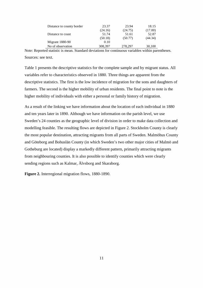
Distance to county border 23.37 23.94 18.15 (24.16) (24.75) (17.00) Distance to coast 51.74 51.61 52.87 (50.18) (50.77) (44.34) Migrant 1880-90 0.10 No of observation 308,397 278,297 30,100
Note: Reported statistic is mean. Standard deviations for continuous variables within parentheses.
Sources: see text.
Table 1 presents the descriptive statistics for the complete sample and by migrant status. All
variables refer to characteristics observed in 1880. Three things are apparent from the
descriptive statistics. The first is the low incidence of migration for the sons and daughters of
farmers. The second is the higher mobility of urban residents. The final point to note is the
higher mobility of individuals with either a personal or family history of migration.
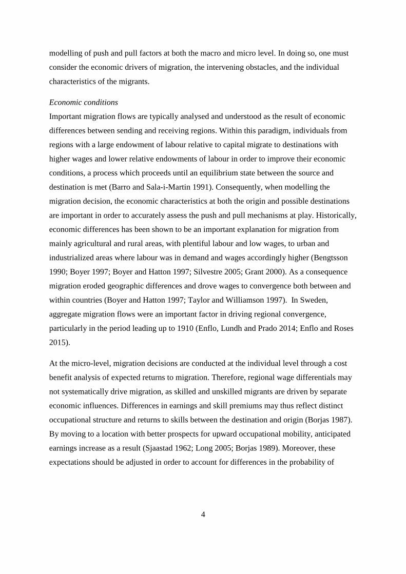
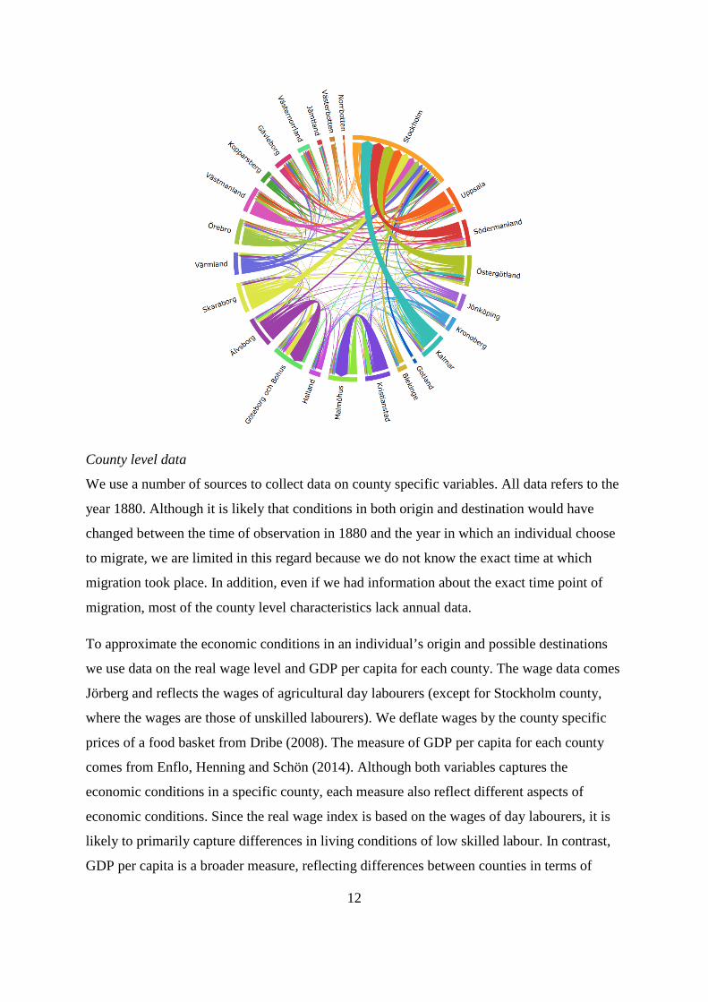
As a result of the linking we have information about the location of each individual in 1880
and ten years later in 1890. Although we have information on the parish level, we use
Sweden’s 24 counties as the geographic level of division in order to make data collection and
modelling feasible. The resulting flows are depicted in Figure 2. Stockholm County is clearly
the most popular destination, attracting migrants from all parts of Sweden. Malmöhus County
and Göteborg and Bohuslän County (in which Sweden’s two other major cities of Malmö and
Gotheburg are located) display a markedly different pattern, primarily attracting migrants
from neighbouring counties. It is also possible to identify counties which were clearly
sending regions such as Kalmar, Älvsborg and Skaraborg.
Figure 2. Interregional migration flows, 1880-1890.
12
County level data
We use a number of sources to collect data on county specific variables. All data refers to the
year 1880. Although it is likely that conditions in both origin and destination would have
changed between the time of observation in 1880 and the year in which an individual choose
to migrate, we are limited in this regard because we do not know the exact time at which
migration took place. In addition, even if we had information about the exact time point of
migration, most of the county level characteristics lack annual data.
To approximate the economic conditions in an individual’s origin and possible destinations
we use data on the real wage level and GDP per capita for each county. The wage data comes
Jörberg and reflects the wages of agricultural day labourers (except for Stockholm county,
where the wages are those of unskilled labourers). We deflate wages by the county specific
prices of a food basket from Dribe (2008). The measure of GDP per capita for each county
comes from Enflo, Henning and Schön (2014). Although both variables captures the
economic conditions in a specific county, each measure also reflect different aspects of
economic conditions. Since the real wage index is based on the wages of day labourers, it is
likely to primarily capture differences in living conditions of low skilled labour. In contrast,
GDP per capita is a broader measure, reflecting differences between counties in terms of

13
economic development. To ease the interpretation and comparison of the estimates of wages
and GDP we use standardised variables (mean = 0, s.d.= 1) when estimating our migration
models.
The degree of urbanisation of each county has been calculated using the complete census of
1880 and is reported as the share of the population in each county that resided in an urban
area. The area of each county comes from BISOS I (1881) and is measure in Swedish square
miles (approximately equal to 106.89 km2). Information about access to transportation has
been collected from official statistics. The data on railways can be found in BISOS L (1881)
and the data on roads in BISOS H (1884). Both are measured as kilometres of road/railway
per Swedish square mile. The data on roads only include public roads, while the railroad data
includes both public and privately owned railways. Two variables, distance and the historical
migration stream, are constructed based on specific information about the origin and a
possible destination and are thus different for each unique combination of county of origin
and potential destination. Distance has been calculated as the number of kilometres between
the centroid of the origin of each county. Similarly, the migration stream variable has been
calculated for each county by identifying all individual living outside their county of birth
according to the 1880 census, and then calculating the share residing in each possible
destination.
The county level characteristics are presented in table 2. In terms of economic conditions
there is considerable variation between counties. Real wages are more than twice as high in
the best paying region compared to the lowest paying. GDP per capita displays a similar
pattern in terms of the variation in regional development. Wages and GDP are, as may be
expected, positively correlated (0.18 and 0.04 for male and female wages respectively)
although not very strongly.
Table 2. County level variables
County code County
Male real wages
Female real wages
GDP per capita
Urban population
share
Share employed in agriculture
1 Stockholms län 112.50 53.75 607.4 56.2 11.9 3 Uppsala län 118.96 59.37 347.6 16.4 21.9 4 Södermanlands län 112.95 61.83 335.2 11.4 26.1 5 Östergötlands län 95.14 60.65 337.8 15.4 21.9 6 Jönköpings län 118.55 60.81 315 10.4 28.7 7 Kronobergs län 139.44 77.31 258.6 2.9 30.8 8 Kalmar län 106.35 51.34 282 10.4 21.5
14
9 Gotlands län 118.51 63.73 322.1 12.7 23.2 10 Blekinge län 96.67 59.21 299.5 19.1 23.1 11 Kristianstads län 146.52 65.82 279.4 5.7 28.2 12 Malmöhus län 100.43 57.85 403.3 24.1 22.5 13 Hallands län 124.66 73.30 276.4 11.2 31.0 14 Göteborg och Bohus län 81.47 56.48 381.1 33.7 20.2 15 Älvsborgs län 101.36 59.15 240.4 5.7 29.7 16 Skaraborgs län 110.74 75.79 295.1 6.9 28.5 17 Värmlands län 76.87 40.68 266.8 5.9 28.6 18 Örebro län 99.01 58.24 283.4 9.1 25.5 19 Västmanlands län 95.33 56.46 365.8 13.9 23.7 20 Kopparbergs län 103.50 59.80 315.1 4.9 27.9 21 Gävleborgs län 130.41 60.10 475.1 17.4 19.7 22 Västernorrlands län 152.19 69.07 392.9 8.6 22.8 23 Jämtlands län 182.14 94.19 415.8 3.4 29.7 24 Västerbottens län 167.10 80.21 313.7 3.5 29.8 25 Norrbottens län 152.38 87.91 407.4 7.2 30.9
Sources: see text
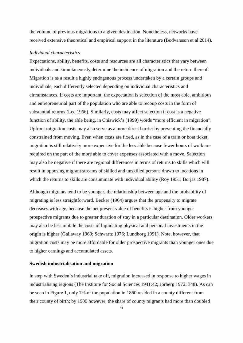
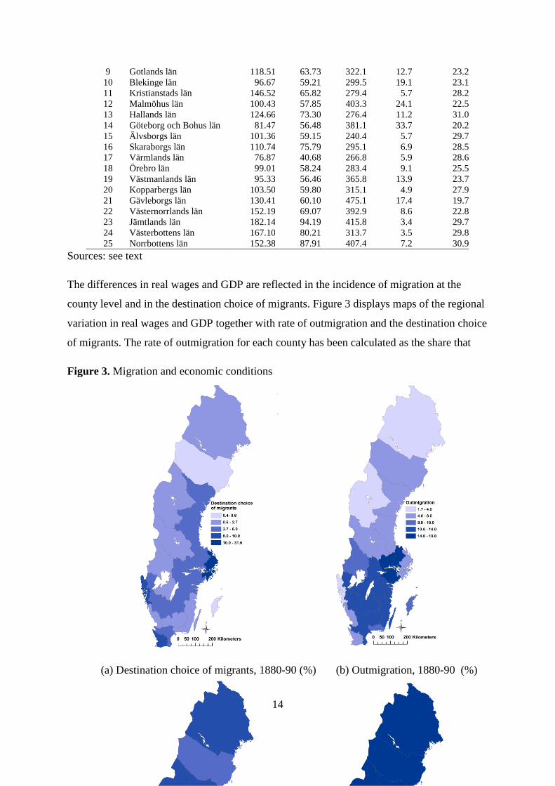
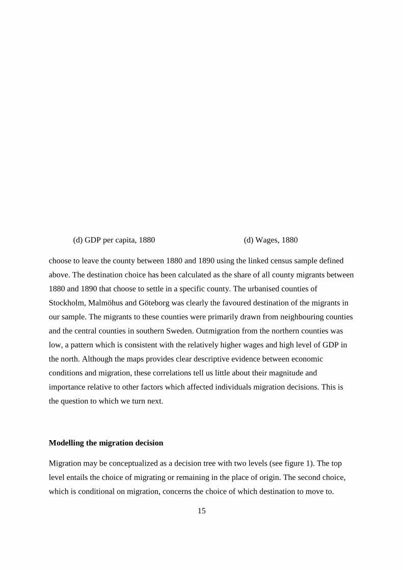
The differences in real wages and GDP are reflected in the incidence of migration at the
county level and in the destination choice of migrants. Figure 3 displays maps of the regional
variation in real wages and GDP together with rate of outmigration and the destination choice
of migrants. The rate of outmigration for each county has been calculated as the share that
Figure 3. Migration and economic conditions
d
sa
(a) Destination choice of migrants, 1880-90 (%) (b) Outmigration, 1880-90 (%)
15
(d) GDP per capita, 1880 (d) Wages, 1880
choose to leave the county between 1880 and 1890 using the linked census sample defined
above. The destination choice has been calculated as the share of all county migrants between
1880 and 1890 that choose to settle in a specific county. The urbanised counties of
Stockholm, Malmöhus and Göteborg was clearly the favoured destination of the migrants in
our sample. The migrants to these counties were primarily drawn from neighbouring counties
and the central counties in southern Sweden. Outmigration from the northern counties was
low, a pattern which is consistent with the relatively higher wages and high level of GDP in
the north. Although the maps provides clear descriptive evidence between economic
conditions and migration, these correlations tell us little about their magnitude and
importance relative to other factors which affected individuals migration decisions. This is
the question to which we turn next.
Modelling the migration decision
Migration may be conceptualized as a decision tree with two levels (see figure 1). The top
level entails the choice of migrating or remaining in the place of origin. The second choice,
which is conditional on migration, concerns the choice of which destination to move to.

16
Figure 3. Two tier nested structure of migration and destination choice
Mobility (m):
m1: stay
m2: move
m1 m2 Destination choice (l):
lo: origin location
lj: migration location, l= 1,2, …,j
lo l1 l2 l3 lj
To account for the fact that destination choice is nested within the migration branch of the
decision tree, thus making destination choice conditional on migration, we employ the utility
maximizing nested logit model developed by McFadden (1978; 1981, 1984). The nested logit
is a less restrictive alternative to the multinomial logit model since the independence of
irrelevant alternatives (IIA) assumption is relaxed. The IIA assumption requires the response
elasticities of choices to be equal. In our case, the use of a multinomial logit model and the
associated IIA assumption would mean that the introduction of a new destination would
require an equal decrease the predicted probability of choosing a specific destination location
and remaining in the origin. By nesting the destination choice within the migration decision,
the IIA assumption only needs to hold between the choice to migrate or not or between
choosing a specific location, and not across the two choice sets. Moreover, the model allows
us to simultaneously assess both the push and pull factors which affect migration. By using
this approach, push factors are evaluated in a binomial migration choice model and pull
factors are assessed in a multinomial destination choice model. This allows for individuals to
value the conditions in the origin differently from those in the destination. Although the
choice is conceptualized as sequential in the decision tree, the nested logit does not impose a
sequential decision process. Or in other words, the model does not imply the unrealistic
assumption that an individual first chooses whether to migrate or not, and only thereafter
considers which destination to choose. The two equations are estimated simultaneously using
maximum likelihood.
17
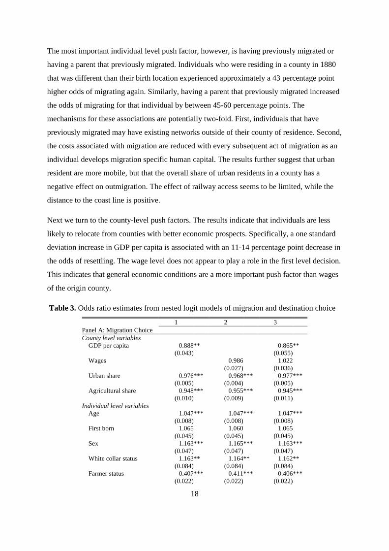
Results
The results from the regression analysis are to be interpreted in the two levels as specified in
the decision tree. The top panel in Table 3 presents the results corresponding to the first level
decision, the push factors that are associated with the decision whether to migrate or remain
in the origin.3 In this case, individual characteristics, as well as the conditions in the origin
county influence the decision to migrate or stay. The lower panel in table 3 displays the
impact of the pull factors, the characteristics of the destination counties that influenced the
destination choice. In general, the results are entirely consistent with theoretical expectations.
In order to understand the economic mechanisms that drive the migration decision, we
estimate 3 model specifications. Model one only contains GDP per capita of the origin and
destination counties, to understand the relationship between the broader macro-economic
conditions and migration decisions. Model two, on the other hand, includes wages in the
origin and destination counties in order to understand whether migration decisions are driven
by labour market conditions. Finally, Model 3 contains both GDP per capita and wages. The
final model specification is used to test whether different economic factors exert a push or
pull force on migration decisions.
Push factors:
The top panel in table 3 present the results of the individual and contextual push factors, the
first level decision. The results indicate that females and individuals residing in urban origins
experience higher odds of choosing to migrate across each of the models. Additionally, a one
year increase in age is associated with roughly a 5 percentage point increase in the odds of
choosing to migrate. The magnitude of the coefficient for age is large, because the sample is
restricted to individuals that are 10 to 20 years of age in 1880, with the higher age groups
being the most likely to migrate. Father’s social status also seems to exert an important push
force. Children of farmers display a roughly 60 percentage point lower odds of choosing to
relocate, while those of white collar workers display a 16 percentage point higher odds
compared to those with skilled fathers.
3 The model has been estimated using a 10% sample. We intend to estimate all models using the full sample. When using the
full sample it does however take more than 24 hours for the maximum likelihood estimation to converge…
18
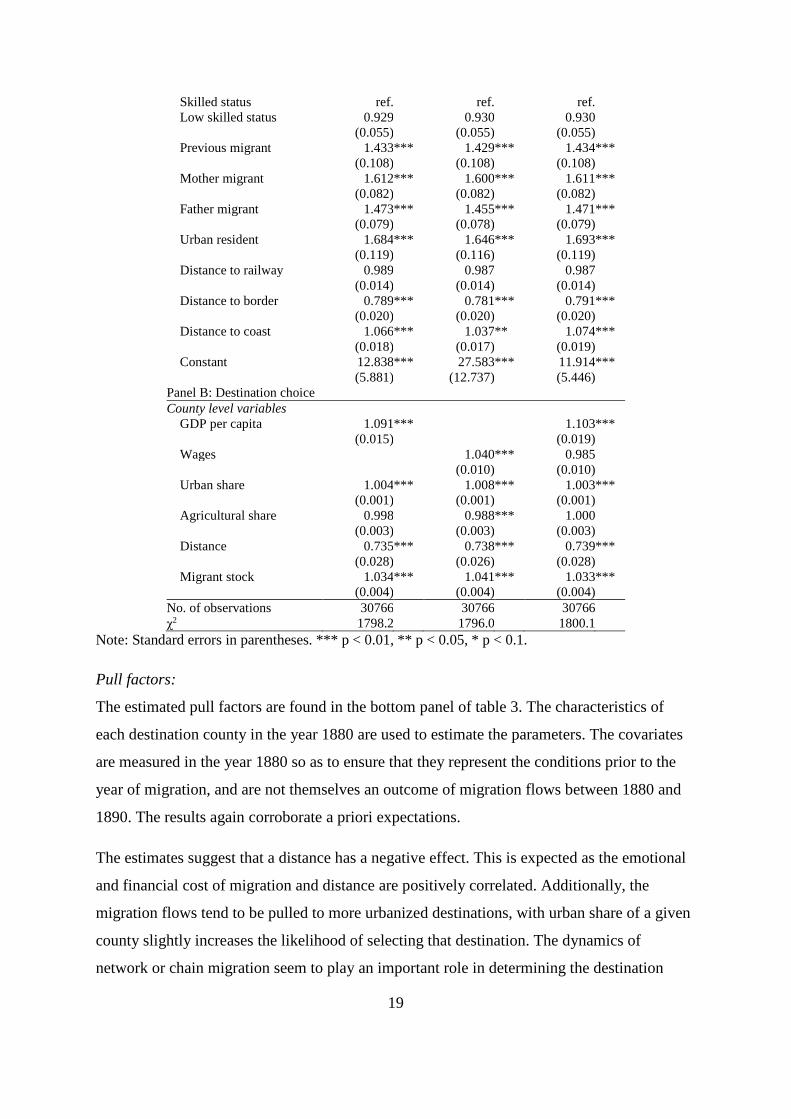
The most important individual level push factor, however, is having previously migrated or
having a parent that previously migrated. Individuals who were residing in a county in 1880
that was different than their birth location experienced approximately a 43 percentage point
higher odds of migrating again. Similarly, having a parent that previously migrated increased
the odds of migrating for that individual by between 45-60 percentage points. The
mechanisms for these associations are potentially two-fold. First, individuals that have
previously migrated may have existing networks outside of their county of residence. Second,
the costs associated with migration are reduced with every subsequent act of migration as an
individual develops migration specific human capital. The results further suggest that urban
resident are more mobile, but that the overall share of urban residents in a county has a
negative effect on outmigration. The effect of railway access seems to be limited, while the
distance to the coast line is positive.
Next we turn to the county-level push factors. The results indicate that individuals are less
likely to relocate from counties with better economic prospects. Specifically, a one standard
deviation increase in GDP per capita is associated with an 11-14 percentage point decrease in
the odds of resettling. The wage level does not appear to play a role in the first level decision.
This indicates that general economic conditions are a more important push factor than wages
of the origin county.
Table 3. Odds ratio estimates from nested logit models of migration and destination choice
1 2 3 Panel A: Migration Choice County level variables
GDP per capita 0.888 ** 0.865 ** (0.043) (0.055)
Wages 0.986 1.022 (0.027) (0.036)
Urban share 0.976 *** 0.968 *** 0.977 *** (0.005) (0.004) (0.005)
Agricultural share 0.948 *** 0.955 *** 0.945 *** (0.010) (0.009) (0.011) Individual level variables
Age 1.047 *** 1.047 *** 1.047 *** (0.008) (0.008) (0.008)
First born 1.065 1.060 1.065 (0.045) (0.045) (0.045)
Sex 1.163 *** 1.165 *** 1.163 *** (0.047) (0.047) (0.047)
White collar status 1.163 ** 1.164 ** 1.162 ** (0.084) (0.084) (0.084) Farmer status 0.407 *** 0.411 *** 0.406 *** (0.022) (0.022) (0.022)
19
Skilled status ref. ref. ref. Low skilled status 0.929 0.930 0.930
(0.055) (0.055) (0.055) Previous migrant 1.433 *** 1.429 *** 1.434 *** (0.108) (0.108) (0.108) Mother migrant 1.612 *** 1.600 *** 1.611 *** (0.082) (0.082) (0.082) Father migrant 1.473 *** 1.455 *** 1.471 ***
(0.079) (0.078) (0.079) Urban resident 1.684 *** 1.646 *** 1.693 ***
(0.119) (0.116) (0.119) Distance to railway 0.989 0.987 0.987
(0.014) (0.014) (0.014) Distance to border 0.789 *** 0.781 *** 0.791 ***
(0.020) (0.020) (0.020) Distance to coast 1.066 *** 1.037 ** 1.074 ***
(0.018) (0.017) (0.019) Constant 12.838 *** 27.583 *** 11.914 ***
(5.881) (12.737) (5.446) Panel B: Destination choice County level variables
GDP per capita 1.091 *** 1.103 *** (0.015) (0.019)
Wages 1.040 *** 0.985 (0.010) (0.010)
Urban share 1.004 *** 1.008 *** 1.003 *** (0.001) (0.001) (0.001)
Agricultural share 0.998 0.988 *** 1.000 (0.003) (0.003) (0.003)
Distance 0.735 *** 0.738 *** 0.739 *** (0.028) (0.026) (0.028)
Migrant stock 1.034 *** 1.041 *** 1.033 *** (0.004) (0.004) (0.004) No. of observations 30766 30766 30766 χ2 1798.2 1796.0 1800.1
Note: Standard errors in parentheses. *** p < 0.01, ** p < 0.05, * p < 0.1.
Pull factors:
The estimated pull factors are found in the bottom panel of table 3. The characteristics of
each destination county in the year 1880 are used to estimate the parameters. The covariates
are measured in the year 1880 so as to ensure that they represent the conditions prior to the
year of migration, and are not themselves an outcome of migration flows between 1880 and
1890. The results again corroborate a priori expectations.
The estimates suggest that a distance has a negative effect. This is expected as the emotional
and financial cost of migration and distance are positively correlated. Additionally, the
migration flows tend to be pulled to more urbanized destinations, with urban share of a given
county slightly increases the likelihood of selecting that destination. The dynamics of
network or chain migration seem to play an important role in determining the destination
20
location. Network theories of migration postulate that existing migrant networks decrease the
cost of migration by providing access to housing or labour market opportunities. Although we
are unable to identify the channel through which this relationship exists, the results indicate
that a 1 percent increase in the origin migrant stock leads to a 3-4 percentage point increase in
the odds of selecting that given location.
The final pull factor tested in our models are the economic conditions in each given
destination. Similar to the push factors, we first test a model that includes GDP per capita.
According to model 1, a one standard deviation increase in wages was associated with a 9
percentage point increase in the odds of selecting a given destination. This model suggests
that broader macroeconomic conditions may be an important pull factor. In model 2, we
replace GDP per capita with wages for each destination location. In this model, the results
indicates that a one standard deviation increase in wages increases the odds of selecting a
given destination by 4 percentage points. The final model which includes both wages as well
as GDP per capita suggests that wages are not an important pull factor relative to GDP.
Rather general economic conditions seem to drive destination selection. The magnitude of the
estimate for GDP per capita remains unchanged from model 2, while the estimate for wages
are no longer statistically significant.
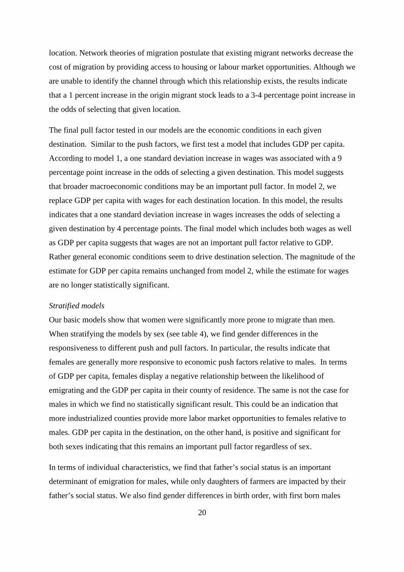
Stratified models
Our basic models show that women were significantly more prone to migrate than men.
When stratifying the models by sex (see table 4), we find gender differences in the
responsiveness to different push and pull factors. In particular, the results indicate that
females are generally more responsive to economic push factors relative to males. In terms
of GDP per capita, females display a negative relationship between the likelihood of
emigrating and the GDP per capita in their county of residence. The same is not the case for
males in which we find no statistically significant result. This could be an indication that
more industrialized counties provide more labor market opportunities to females relative to
males. GDP per capita in the destination, on the other hand, is positive and significant for
both sexes indicating that this remains an important pull factor regardless of sex.
In terms of individual characteristics, we find that father’s social status is an important
determinant of emigration for males, while only daughters of farmers are impacted by their
father’s social status. We also find gender differences in birth order, with first born males
21
being more likely to emigrate relative to later born children, but no such relationship for
females. This may indicate that first born females play a more important role in terms of
household labor.
The models stratified by sex shed light on the result that females are more migratory than
males and that the reason may be that females were more responsive to push factors when it
comes to internal migration. This reflects the claims of Ravenstein (1885, 1889) that females
are more internally migratory, while males more likely to migrate internationally.
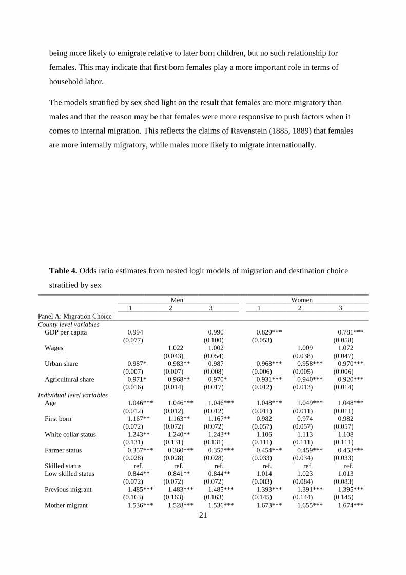
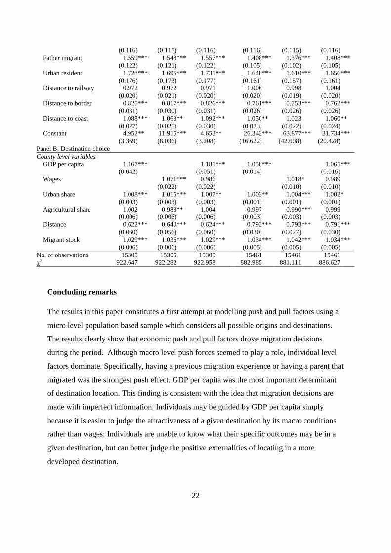
Table 4. Odds ratio estimates from nested logit models of migration and destination choice
stratified by sex
Men Women 1 2 3 1 2 3
Panel A: Migration Choice County level variables
GDP per capita 0.994 0.990 0.829 *** 0.781 *** (0.077) (0.100) (0.053) (0.058)
Wages 1.022 1.002 1.009 1.072 (0.043) (0.054) (0.038) (0.047)
Urban share 0.987 * 0.983 ** 0.987 0.968 *** 0.958 *** 0.970 *** (0.007) (0.007) (0.008) (0.006) (0.005) (0.006)
Agricultural share 0.971 * 0.968 ** 0.970 * 0.931 *** 0.940 *** 0.920 *** (0.016) (0.014) (0.017) (0.012) (0.013) (0.014) Individual level variables
Age 1.046 *** 1.046 *** 1.046 *** 1.048 *** 1.049 *** 1.048 *** (0.012) (0.012) (0.012) (0.011) (0.011) (0.011)
First born 1.167 ** 1.163 ** 1.167 ** 0.982 0.974 0.982 (0.072) (0.072) (0.072) (0.057) (0.057) (0.057)
White collar status 1.243 ** 1.240 ** 1.243 ** 1.106 1.113 1.108 (0.131) (0.131) (0.131) (0.111) (0.111) (0.111) Farmer status 0.357 *** 0.360 *** 0.357 *** 0.454 *** 0.459 *** 0.453 *** (0.028) (0.028) (0.028) (0.033) (0.034) (0.033) Skilled status ref. ref. ref. ref. ref. ref. Low skilled status 0.844 ** 0.841 ** 0.844 ** 1.014 1.023 1.013
(0.072) (0.072) (0.072) (0.083) (0.084) (0.083) Previous migrant 1.485 *** 1.483 *** 1.485 *** 1.393 *** 1.391 *** 1.395 *** (0.163) (0.163) (0.163) (0.145) (0.144) (0.145) Mother migrant 1.536 *** 1.528 *** 1.536 *** 1.673 *** 1.655 *** 1.674 ***
22
(0.116) (0.115) (0.116) (0.116) (0.115) (0.116) Father migrant 1.559 *** 1.548 *** 1.557 *** 1.408 *** 1.376 *** 1.408 ***
(0.122) (0.121) (0.122) (0.105) (0.102) (0.105) Urban resident 1.728 *** 1.695 *** 1.731 *** 1.648 *** 1.610 *** 1.656 ***
(0.176) (0.173) (0.177) (0.161) (0.157) (0.161) Distance to railway 0.972 0.972 0.971 1.006 0.998 1.004
(0.020) (0.021) (0.020) (0.020) (0.019) (0.020) Distance to border 0.825 *** 0.817 *** 0.826 *** 0.761 *** 0.753 *** 0.762 ***
(0.031) (0.030) (0.031) (0.026) (0.026) (0.026) Distance to coast 1.088 *** 1.063 ** 1.092 *** 1.050 ** 1.023 1.060 **
(0.027) (0.025) (0.030) (0.023) (0.022) (0.024) Constant 4.952 ** 11.915 *** 4.653 ** 26.342 *** 63.877 *** 31.734 ***
(3.369) (8.036) (3.208) (16.622) (42.008) (20.428) Panel B: Destination choice County level variables
GDP per capita 1.167 *** 1.181 *** 1.058 *** 1.065 *** (0.042) (0.051) (0.014) (0.016)
Wages 1.071 *** 0.986 1.018 * 0.989 (0.022) (0.022) (0.010) (0.010)
Urban share 1.008 *** 1.015 *** 1.007 ** 1.002 ** 1.004 *** 1.002 * (0.003) (0.003) (0.003) (0.001) (0.001) (0.001)
Agricultural share 1.002 0.988 ** 1.004 0.997 0.990 *** 0.999 (0.006) (0.006) (0.006) (0.003) (0.003) (0.003)
Distance 0.622 *** 0.640 *** 0.624 *** 0.792 *** 0.793 *** 0.791 *** (0.060) (0.056) (0.060) (0.030) (0.027) (0.030)
Migrant stock 1.029 *** 1.036 *** 1.029 *** 1.034 *** 1.042 *** 1.034 *** (0.006) (0.006) (0.006) (0.005) (0.005) (0.005) No. of observations 15305 15305 15305 15461 15461 15461 χ2 922.647 922.282 922.958 882.985 881.111 886.627
Concluding remarks
The results in this paper constitutes a first attempt at modelling push and pull factors using a
micro level population based sample which considers all possible origins and destinations.
The results clearly show that economic push and pull factors drove migration decisions
during the period. Although macro level push forces seemed to play a role, individual level
factors dominate. Specifically, having a previous migration experience or having a parent that
migrated was the strongest push effect. GDP per capita was the most important determinant
of destination location. This finding is consistent with the idea that migration decisions are
made with imperfect information. Individuals may be guided by GDP per capita simply
because it is easier to judge the attractiveness of a given destination by its macro conditions
rather than wages: Individuals are unable to know what their specific outcomes may be in a
given destination, but can better judge the positive externalities of locating in a more
developed destination.
23
The implications of these are important to the literature as they are consistent with existing
theories of migration. The validity of theoretical push and pull factors are uncompromised
when comprehensively modelling the decision process. More work remains to be done in
order to identify the mechanisms through which some of these factors are operating.
It is important to note that this paper does not explicitly test individual level pull factors,
which theoretically must exist, but we intend to address this at a later time. One important
individual level pull factor is the existence of specific kin-based networks. Although our
results indicate that networks are an important pull factor, at what level networks matter. We
intend to disentangle this effect further by capturing networks at a more detailed level in the
future.
References (Incomplete! Needs to be checked!)
Baines, D. (1985). Migration in a Mature Economy: Emigration and Internal Migration in
England and Wales 1861-1900. Cambridge: University Press.
Bengtsson, T. 1990
Berger, T. and Enflo, K. (2013). Locomotives of local growth: the short- and long-term
impact of railroads in Sweden, EHES Working Papers in Economic History, 42.
Bidrag till Sveriges Officiella Statistik. H) Kungl. Maj:ts befallnings-havandes
fem-årsberättelser 1976-1880. (1884)
Bidrag till Sveriges Officiella Statistik. I) Telegrafväsendet 1880. (1881)
Bidrag till Sveriges Officiella Statistik. L) Statens Järnvägstrafik 1880. (1881)
Borjas, G. J. (1987). Self-selection and the earnings of immigrants. American Economic
Review, 77: 531-553.
24
Boyer, G.R. (1997). Labour migration in southern and eastern England, European Review of
Economic History, 1: 191-215
Boyer, G.R. and Hatton, T.J. (1997). Migration and labour market integration late nineteenth-
century England and Wales, Economic History Review, 50: 697-734.
Brändström, A., Sundin, J. and Tedebrand, L-G. (2012). Two Cities: Urban Migration and
Settlement in Nineteenth-century Sweden. The History of the Family, 5: 415-29.
Chiswick, B. (1999). Are immigrants favorably self-selected? The American Economic
Review, 89: 181-185.
Clark, P. (1979). Migration in England during the Late Seventeenth and Early Eighteenth
Centuries. Past & Present, 83: 57-90.
Devine, T.M. (1979). Temporary Migration and the Scottish Highlands in the Nineteenth
Century. The Economic History Review. 32: 344-59.
Dribe, M. (2000). Leaving home in a peasant society. Economic fluctuations, household
dynamics and youth migration in southern Sweden, 1829-1866. Södertälje: Almqvist &
Wiksell International.
Dribe, M. (2003). Migration of rural families in 19th century southern Sweden. A longitudinal
analysis of local migration patterns. The History of the Family, 8: 247-65.
Dribe, M. (2008). Demand and supply factors in the fertility transition: A county level
analysis of age-specific marital fertility in Sweden 1880-1930. European Review of
Economic History, 13: 65-94.
Dribe, M. and Lundh, C. (2005). People on the move: determinants of servant Migration in
nineteenth-century Sweden. Continuity and Change, 20: 53-91.
Enflo K, Henning M. and Schön L. (2014). Swedish regional GDP 1855-2000: Estimations
and general trends in the Swedish regional system. Research in Economic History, 30:
47-89.
Enflo, K. and Roses, J.R. (2015). Coping with regional inequality in Sweden: structural
change, migrations, and policy, 1860-2000. The Economic History Review, 1: 191-217.
25
Enflo, K., Lundh, C. and Prado, S. (2014). The role of migration in regional wage
convergence: Evidence from Sweden 1860-1940. Explorations in Economic History, 52:
93-110.
Eriksson, B. (2015). Dynamic Decades: A micro perspective on late nineteenth century
Sweden, Lund: Media-Tryck.
Eriksson, B. (2016) False positives and faulty estimates: Linked census data and bias to
estimates of social mobility, unpublished manuscript.
Eriksson, I. and Rogers, J. (1978). Rural Labor and Population Change. Stockholm:
Almqvist & Wiksell.
Gaunt, D. (1977). Pre-industrial Economy and Population Structure. Scandinavian Journal of
History, 2: 183-210.
Geschwind, A. and Fogelvik, S. (2000). The Stockholm Historical Database. In P.K. Hall, R.
McCaa, G. Thorvaldsen (eds.), Handbook of International Historical Microdata for
Population Research, pp. 207 – 231. Minneapolis: Minnesota Population Center.
Harris, J.R. and Todaro, M.P. (1970). Migration, Unemployment and Development: A Two-
Sector Analysis, American Economic Review, 60: 126–142
Hochstadt, S. (1983). Migration in Preindustrial Germany. Central European History, 16:
195-224.
Jackson, J.H. and Moch, L.P. (1989). Migration and the Social History of Modern Europe.
Historical Methods, 22: 27-36.
Jörberg, L. (1972). A History of Prices in Sweden 1732-1914. Vol. 2, Lund: CWK Gleerup.
Lee, E.S. (1966) A Theory of Migration, Demography, 3: 47-57.
Long, J. (2005). Rural-Urban Migration and Socioeconomic Mobility in Victorian Britain.
The Journal of Economic History, 65: 1-35.
Lundh, C. (1999). Servant Migration in Sweden in the Early Nineteenth Century. Journal of
Family History, 24: 53-74.
26
Lundh, C. (2003). Life Cycle Servants in Nineteenth Century Sweden – Norms and Practice.
Lund Papers in Economic History, No. 84.
McFadden, D. (1978). Modelling the choice of residential location, (pp.75-96) in A.
Karlquist, L. Lundquist, F. Snickars, and J.W. Weibull (Eds.), Spatial interaction theory
and planning models. Amsterdam: North Holland.
McFadden, D. (1981). Econometric models of probabilistic choice, (pp. 198-272) in C.F.
Manski and D, McFAdden (Eds.), Structural analysis of discrete data with econometric
applications. Cambridge: MIT Press.
Moch, L.P. (1992). Moving Europeans: Migration in Western Europe since 1650.
Bloomington: Indiana University Press.
Parish, W.L. (1973). Internal Migration and Modernization: The European Case. Economic
Development and Cultural Change, 21: 591-609.
Patten, J. (1976). Patterns of migration and movement of labour of three preindustrial East
Anglian towns. Journal of Historical Geography. 2: 111-29.
Pryor, R.J. (1975). Migration and the process of modernization. pp. 23-38, in Kosinski, L.A.
& Prothero, R.M. People on the Move. London: Methuen & Co.
Ravenstein, E.G. (1889). The Laws of Migration: Second Paper. Journal of the Royal
Statistical Society, 52: 241-305.
Roy, A. D. (1951). Some thoughts on the distribution of earnings. Oxford Economic Papers,
3: 135-146.
Schön, L. (2010). Sweden’s Road to Modernity: An Economic History, Stockholm: SNS.
Schwartz, A. (1973). Interpreting the effect of distance on migration, Journal of Political
Economy, 81: 1153-1169.
Sjastaad, L.A. (1962). The Costs and Returns of Human Migration. Journal of Political
Economy, 70: 80-93.
Statistiska Centralbyrån (1969). Historisk statistik för Sverige, 1, Stockholm.
27
Taylor, A.M. and Williamson, J.G. (1997). Convergence in the age of mass migration,
European Review of Economic History, 1: 27-63.
The Institute for Social Sciences, Stockholm University, (1941). Population Movements and
Industrialization. London: P.S. King & Son.
Thomas, D.S. (1941). Social and Economic Aspects of the Swedish Population Movement,
1750-1933. New York: The Macmillan Company.
van der Woude, A., Hayami, A. and Vries, J. (1990). Urbanization in History. Oxford:
Clarendon Press.
van Leeuwen, M. H. D. and Maas, I. (2011). HISCLASS. A historical international social
class scheme. Leuven: Leuven University Press.
van Leeuwen, M. H. D., Maas, I., and Miles, A. (2002). HISCO. Historical international
standard classification of occupations. Leuven: Leuven University Press.
Zelinsky, W. (1971). The Hypothesis of the Mobility Transition. Geographical Review, 61:
219-49.
Hicks, J.R. (1932): The theory of wages. London: Macmillan

28
Appendix
Table A1. Odds ratio estimates from nested logit models of migration and destination choice
stratified by SES
White collar Farmer 1 2 3 1 2 3
Panel A: Migration Choice County level variables
GDP per capita 0.941 0.963 0.873 *** 0.822 *** (0.040) (0.054) (0.022) (0.027)
Wages 0.971 0.975 1.011 1.057 *** (0.025) (0.033) (0.014) (0.019)
Urban share 0.979 *** 0.975 *** 0.978 *** 0.999 0.989 *** 1.002 (0.004) (0.004) (0.004) (0.003) (0.002) (0.003)
Agricultural share 0.959 *** 0.965 *** 0.963 *** 0.972 *** 0.976 *** 0.964 *** (0.009) (0.008) (0.010) (0.005) (0.005) (0.005) Individual level variables
Age 1.057 *** 1.057 *** 1.057 *** 1.059 *** 1.059 *** 1.059 *** (0.007) (0.007) (0.007) (0.004) (0.004) (0.004)
First born 1.003 1.000 1.003 0.991 0.985 0.990 (0.039) (0.039) (0.039) (0.021) (0.021) (0.021)
Sex 0.837 *** 0.837 *** 0.837 *** 1.208 *** 1.211 *** 1.207 *** (0.031) (0.031) (0.031) (0.024) (0.024) (0.024)
Previous migrant 1.906 *** 1.907 *** 1.906 *** 1.666 *** 1.660 *** 1.667 *** (0.097) (0.097) (0.096) (0.075) (0.075) (0.076) Mother migrant 1.483 *** 1.477 *** 1.483 *** 1.486 *** 1.482 *** 1.487 *** (0.063) (0.063) (0.063) (0.040) (0.040) (0.040) Father migrant 1.420 *** 1.414 *** 1.420 *** 1.665 *** 1.653 *** 1.665 ***
(0.060) (0.059) (0.060) (0.051) (0.050) (0.051) Urban resident 1.330 *** 1.308 *** 1.329 *** 2.004 *** 2.021 *** 2.002 ***
(0.065) (0.063) (0.065) (0.165) (0.166) (0.164) Distance to railway 1.008 1.008 1.007 0.959 *** 0.958 *** 0.958 ***
29
(0.012) (0.012) (0.012) (0.007) (0.007) (0.007) Distance to border 0.951 ** 0.948 ** 0.951 ** 0.793 *** 0.780 *** 0.795 ***
(0.023) (0.022) (0.023) (0.010) (0.009) (0.010) Distance to coast 1.023 * 1.005 1.022 1.055 *** 1.016 * 1.064 ***
(0.013) (0.012) (0.014) (0.010) (0.010) (0.011) Constant 5.361 *** 8.563 *** 5.023 *** 5.729 *** 16.211 *** 6.113 ***
(2.127) (3.421) (1.981) (1.381) (3.936) (1.510) Panel B: Destination choice County level variables
GDP per capita 1.073 *** 1.095 *** 1.123 *** 1.096 *** (0.015) (0.019) (0.009) (0.010)
Wages 1.025 *** 0.976 ** 1.086 *** 1.030 *** (0.009) (0.011) (0.007) (0.007)
Urban share 1.009 *** 1.012 *** 1.008 *** 1.002 *** 1.007 *** 1.003 *** (0.001) (0.002) (0.001) (0.001) (0.001) (0.001)
Agricultural share 0.999 0.992 *** 1.002 0.994 *** 0.980 *** 0.990 *** (0.003) (0.003) (0.003) (0.002) (0.002) (0.002)
Distance 0.713 *** 0.720 *** 0.718 *** 0.669 *** 0.660 *** 0.665 *** (0.032) (0.029) (0.031) (0.014) (0.014) (0.015)
Migrant stock 1.026 *** 1.031 *** 1.026 *** 1.042 *** 1.049 *** 1.042 *** (0.003) (0.003) (0.003) (0.002) (0.002) (0.002) No. of observations 21089 21089 21089 188258 188258 188258 χ2 1385.426 1383.492 1385.594 4937.566 4977.823 4947.502
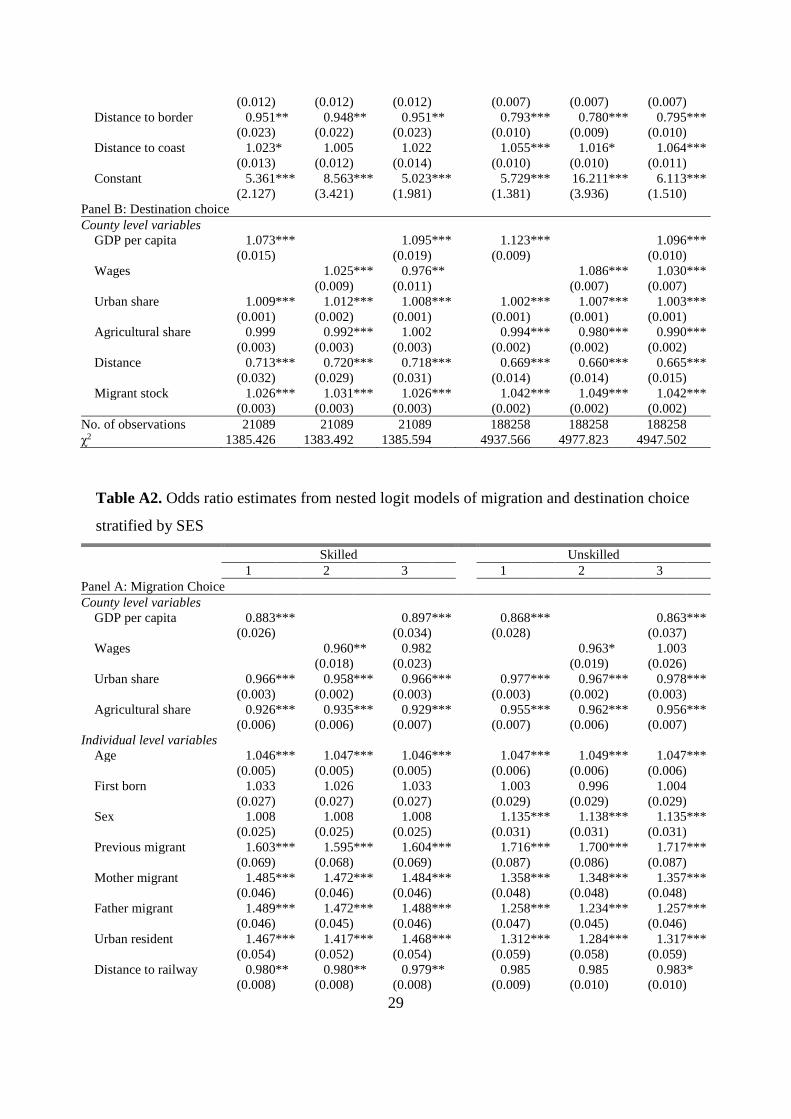
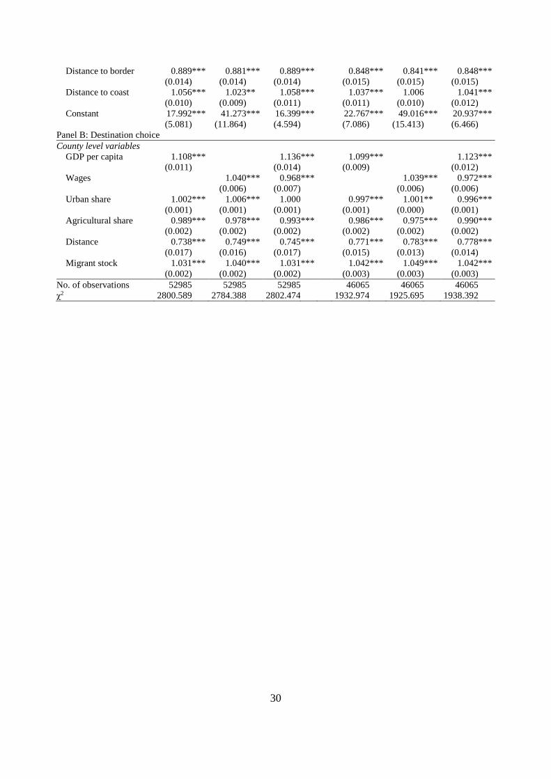
Table A2. Odds ratio estimates from nested logit models of migration and destination choice
stratified by SES
Skilled Unskilled 1 2 3 1 2 3
Panel A: Migration Choice County level variables
GDP per capita 0.883 *** 0.897 *** 0.868 *** 0.863 *** (0.026) (0.034) (0.028) (0.037)
Wages 0.960 ** 0.982 0.963 * 1.003 (0.018) (0.023) (0.019) (0.026)
Urban share 0.966 *** 0.958 *** 0.966 *** 0.977 *** 0.967 *** 0.978 *** (0.003) (0.002) (0.003) (0.003) (0.002) (0.003)
Agricultural share 0.926 *** 0.935 *** 0.929 *** 0.955 *** 0.962 *** 0.956 *** (0.006) (0.006) (0.007) (0.007) (0.006) (0.007) Individual level variables
Age 1.046 *** 1.047 *** 1.046 *** 1.047 *** 1.049 *** 1.047 *** (0.005) (0.005) (0.005) (0.006) (0.006) (0.006)
First born 1.033 1.026 1.033 1.003 0.996 1.004 (0.027) (0.027) (0.027) (0.029) (0.029) (0.029)
Sex 1.008 1.008 1.008 1.135 *** 1.138 *** 1.135 *** (0.025) (0.025) (0.025) (0.031) (0.031) (0.031)
Previous migrant 1.603 *** 1.595 *** 1.604 *** 1.716 *** 1.700 *** 1.717 *** (0.069) (0.068) (0.069) (0.087) (0.086) (0.087) Mother migrant 1.485 *** 1.472 *** 1.484 *** 1.358 *** 1.348 *** 1.357 *** (0.046) (0.046) (0.046) (0.048) (0.048) (0.048) Father migrant 1.489 *** 1.472 *** 1.488 *** 1.258 *** 1.234 *** 1.257 ***
(0.046) (0.045) (0.046) (0.047) (0.045) (0.046) Urban resident 1.467 *** 1.417 *** 1.468 *** 1.312 *** 1.284 *** 1.317 ***
(0.054) (0.052) (0.054) (0.059) (0.058) (0.059) Distance to railway 0.980 ** 0.980 ** 0.979 ** 0.985 0.985 0.983 *
(0.008) (0.008) (0.008) (0.009) (0.010) (0.010)
30
Distance to border 0.889 *** 0.881 *** 0.889 *** 0.848 *** 0.841 *** 0.848 *** (0.014) (0.014) (0.014) (0.015) (0.015) (0.015)
Distance to coast 1.056 *** 1.023 ** 1.058 *** 1.037 *** 1.006 1.041 *** (0.010) (0.009) (0.011) (0.011) (0.010) (0.012)
Constant 17.992 *** 41.273 *** 16.399 *** 22.767 *** 49.016 *** 20.937 *** (5.081) (11.864) (4.594) (7.086) (15.413) (6.466) Panel B: Destination choice County level variables
GDP per capita 1.108 *** 1.136 *** 1.099 *** 1.123 *** (0.011) (0.014) (0.009) (0.012)
Wages 1.040 *** 0.968 *** 1.039 *** 0.972 *** (0.006) (0.007) (0.006) (0.006)
Urban share 1.002 *** 1.006 *** 1.000 0.997 *** 1.001 ** 0.996 *** (0.001) (0.001) (0.001) (0.001) (0.000) (0.001)
Agricultural share 0.989 *** 0.978 *** 0.993 *** 0.986 *** 0.975 *** 0.990 *** (0.002) (0.002) (0.002) (0.002) (0.002) (0.002)
Distance 0.738 *** 0.749 *** 0.745 *** 0.771 *** 0.783 *** 0.778 *** (0.017) (0.016) (0.017) (0.015) (0.013) (0.014)
Migrant stock 1.031 *** 1.040 *** 1.031 *** 1.042 *** 1.049 *** 1.042 *** (0.002) (0.002) (0.002) (0.003) (0.003) (0.003) No. of observations 52985 52985 52985 46065 46065 46065 χ2 2800.589 2784.388 2802.474 1932.974 1925.695 1938.392