Page 1 of 29

Quabbin to Cardigan Conservation Plan

Technical Report 2008

Prepared for the Quabbin to Cardigan Partnership by

Dan Sundquist, Director of Land Conservation Planning

The Society for the Protection of NH Forests

Page 2 of 29

Introduction

This document chronicles the development of the Quabbin to Cardigan strategic conservation plan.

It begins in the early days of the Quabbin to Cardigan project in 2003 when an overarching vision

was crafted by the stakeholders that distilled the shared goal of the Q2C conservation plan: “to

identify and protect large forest blocks with significant embedded ecological features.” In other

words, the region’s mosaic of intact forest blocks would provide the underlying structure for the

plan, and that to the extent that other important natural resources co-occur within that mosaic,

certain forest blocks would be elevated in priority as target areas for concerted conservation efforts.

This later led to the delineation of final “conservation focus areas” and “supporting landscapes” –

which were adopted by the Q2C Partnership in June 2007 -- that reflect actual, on-the-ground

geographies within which Q2C land protection projects should be focused.

PHASE I: Natural Resource Co-Occurrence Mapping, 2004-2005

Overview of GIS Method

The regional scale study of important natural resources in the Q2C involved several discrete steps.

First, wide-ranging research was conducted to develop a database of digital information that could

be used in the GIS for mapping and analysis purposes. It is important to note that funding and time

limits did not permit the development of new and unique datasets; rather, the group agreed that

“best available” data would be used as building blocks in this study. Data was obtained from both

the Massachusetts and New Hampshire GIS data libraries (MassGIS and GRANIT, respectively), as

well as from participating organizations with specialized data, e.g., The Nature Conservancy, and

various state agencies. The data was evaluated for content and accuracy, and then was assembled

into a list by resource type for review by the stakeholder group.

Second, from the list of potential data and illustrative mapping, the group selected a set of resource

factors that best reflected the study goal above, and which are described in detail below. Some data,

such as regional recreation trails, were deemed important to the planning effort, but not suitable for

the next step in the study: the resource co-occurrence analysis. These datasets were set aside as

reference datasets to be overlaid and compared to the results of the co-occurrence analysis in

planning specific projects, or project approaches in the smaller regional venues within the Q2C. In

fact, the regional trails were subsequently analyzed to identify trail segments that should be tagged

as conservation priority targets; this study is detailed later in this report.

The third step in the process was to conduct a co- occurrence analysis of

the data. A co-occurrence model is used in landscape-scale conservation

planning to determine where a variety of natural resource factors are co-

located, thus implying potentially higher conservation values. The diagram

at the right shows schematically how this process works to build a database

of spatial information about any particular location on the ground. This

model is run in the GIS, using numerical values associated with each data

Page 3 of 29

factor. The key to drafting a valid co-occurrence map is how the many data factors are weighted,

especially in terms of the group process used in large stakeholder groups with many areas of natural

resource expertise and interests represented. For the Q2C project, a consensus building process of

anonymous voting termed a Delphi process was used to craft both a shared vision of the relative

importance values associated with the range of natural resource factors being evaluated, which also

results in the numerical values that can be used in the GIS.

Data Factors & Rationale

Unfragmented Forest blocks

A forest block is an area of intact forest with continuous canopy,

without regard to ownership. Thus it functions as a structural

matrix for wildlife habitat, with block-to-block connections

being important for the movement of wildlife. Large forest

blocks are also important for the natural management of water

quality and quantity, and as an economic resource to sustainable

forestry. Block edges are defined by highways and local roads,

non-forest land uses, and/or by large water features.

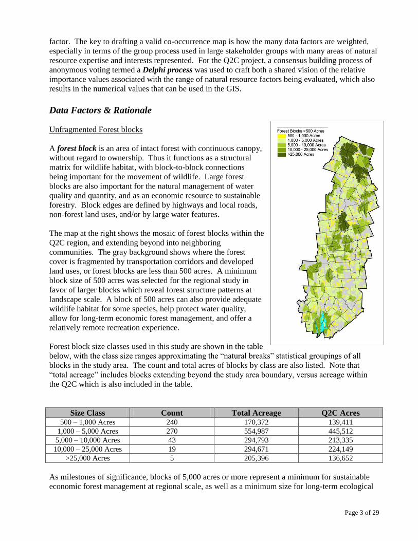
The map at the right shows the mosaic of forest blocks within the

Q2C region, and extending beyond into neighboring

communities. The gray background shows where the forest

cover is fragmented by transportation corridors and developed

land uses, or forest blocks are less than 500 acres. A minimum

block size of 500 acres was selected for the regional study in

favor of larger blocks which reveal forest structure patterns at

landscape scale. A block of 500 acres can also provide adequate

wildlife habitat for some species, help protect water quality,

allow for long-term economic forest management, and offer a

relatively remote recreation experience.

Forest block size classes used in this study are shown in the table

below, with the class size ranges approximating the “natural breaks” statistical groupings of all

blocks in the study area. The count and total acres of blocks by class are also listed. Note that

“total acreage” includes blocks extending beyond the study area boundary, versus acreage within

the Q2C which is also included in the table.

Size Class Count Total Acreage Q2C Acres 500 – 1,000 Acres 240 170,372 139,411

1,000 – 5,000 Acres 270 554,987 445,512

5,000 – 10,000 Acres 43 294,793 213,335

10,000 – 25,000 Acres 19 294,671 224,149

>25,000 Acres 5 205,396 136,652

As milestones of significance, blocks of 5,000 acres or more represent a minimum for sustainable

economic forest management at regional scale, as well as a minimum size for long-term ecological

Page 4 of 29

significance. Blocks greater than 10,000 acres, and especially greater than 25,000 acres, represent

the best scale to ensure that ecological structure, function, and processes such as soil nutrient

accumulation and formation of old growth forests have sufficient framework to foster true

ecological stability over the long term.

Note in the map how the largest forest blocks work to anchor either end of the Q2C study area, with

very large blocks to the north that link to the White Mountain National Forest and another large

block surrounding the Quabbin Reservoir in Massachusetts. Scattered north to south are series of

blocks greater than 10,000 acres in size that follow the height of land between the Connecticut and

Merrimack River watersheds. In New Hampshire, four significant mountains -- Mt. Cardigan, Mt.

Kearsarge, Mt. Sunapee, Mt. Mondanock – and their associated undeveloped forest blocks, serve as

a bio-geographic island chain that links the large anchor blocks north and south.

Intact forest cover of this extent is not common in New Hampshire or Massachusetts, especially east

of the Q2C interest area in both states where the influence of metropolitan Boston has pushed

suburban and exurban development well west and north,

Land cover data from the USGS National Land Cover Dataset (1998) was used as a starting point to

define forest blocks across the two states. This GIS data is developed from satellite imagery using a

30-meter grid; this results in a resolution of about 1/5th

of an acre, but is quite suitable for regional

land use analysis. The land cover data is classified using remote sensing technology to depict a

range of natural land cover types (forest, wetlands, water, etc.) and human uses of the land

(transportation, built-up areas, disturbed areas, etc.). However, the land cover grids are only as

good as the spectral energy seen in the satellite imagery, and therefore represent best

approximations of actual conditions on the ground. An example, important to understanding forest

blocks, is that roads with tree canopy overhead will not be “seen” as transportation features.

Therefore, the land cover data needed to be further processed to define forest blocks.

To do this, data on the road and highway networks for both Massachusetts and New Hampshire

were “burned into” the NLCD land cover grid. To be as accurate as possible, only roads classified

as “traveled” were used in processing the data, with the idea that discontinued rural roads which are

common in New England, and many private roads (actually driveways) included in the GIS data see

little or no disturbance, and therefore do not have a fragmenting effect. However, it was found

early on in evaluating and applying these official state road and highway data that mistakes had

been made in classifying discontinued (so-called Class 6 roads) as functional segments of the local

road system. It was not within the scope of the study to vet the road data in all 3,000 square miles

of study area, so it was agreed to work with the existing data. One exception to that was an effort

made by the North Quabbin Partnership to review and mark up mapping in the Massachusetts

portion of the Q2C study area, and revisions were made to the digital data.

This is an important note because the edges of forest blocks were largely defined by traveled roads

and highways, versus other land uses or large water bodies. This in turn effects the calculation of

block size and classification in the co-occurrence model. But this is also an example of the limits

of best available data in regional studies such as this, and acceptable range of error in the data.

Also see the Core Focus Area Delineation section later in this report for more detail on forested

habitat and the role of forest blocks in the NH Wildlife Action Plan.

Page 5 of 29

Important Forest Soils

Apart from the obvious economic values noted above, forests are also directly linked to the quality

of other natural resources typically considered in natural resource inventory and conservation

planning. The structure, composition, and ecological processes at work in forests are critical to a

myriad of wildlife habitat values. Forests are also integral to maintaining water quality and

regulating water quantity as they relate to both the natural world and to human uses.

While long-term forest management plans seek to maximize all the benefits and uses of our forests,

the innate productivity of any forest is dependant in large part on landscape position (elevation,

topography, etc.), and especially on soil types. These relationships have been well-studied in New

Hampshire, and we are fortunate to have soils mapping that includes groupings of soil types

according to general productivity and forest type.

Three important forest soil groupings are of special note, and are described as follows. These soils

groupings can be thought of as our “most productive forest soils” for the given forest types,

although forest management can and does produce significant economic results on less productive

soils. The characterization of important forest groups varies by county in New Hampshire.

Information on each county soil survey can be found at this link

http://www.nh.nrcs.usda.gov/Soil_Data/soil_data.html. Within each soil survey, a “data dictionary”

discusses typical soils characteristics and forest cover types for each NH forest soil grouping. The

relevant soil surveys for the N.H. portion of the Q2C are Cheshire, Sullivan, Grafton, Hillsborough

and Merrimack counties.

New Hampshire Classification System

The most productive forest soils in New Hampshire are characterized as follows:

Group IA consists of the deeper, loamy, moderately well drained and well drained soils.

Generally, these soils are more fertile and have the most favorable soil moisture

relationships. Successional trends on these soils are toward climax stands of shade tolerant

hardwoods, such as sugar maple and beech. Early successional stands frequently contain a

variety of hardwoods such as sugar maple, beech, red maple, yellow, gray, and white birch,

aspen, white ash, and northern red oak in varying combinations with red and white spruce,

balsam fir, hemlock, and white pine. The soils in this group are well suited for growing high

quality hardwood veneer and saw timber, especially, sugar maple, white ash, yellow birch,

and northern red oak.

Group IB generally consists of soils that are moderately well drained and well drained,

sandy or loamy over sandy, and slightly less fertile than those in group 1A. Soil moisture is

adequate for good tree growth, but may not be quite as abundant as in group1A.

Successional trends and the trees common in early successional stands are similar to those in

group IA. However, beech is usually more abundant on group IB and is the dominant

species in climax stands. Group IB soils are well suited for growing less nutrient and

moisture demanding hardwoods such as white birch and northern red oak. Softwoods

generally are scarce to moderately abundant and managed in groups or as part of a mixed

stand.

Page 6 of 29

Group IC soils are derived from glacial outwash sand and gravel. The soils are coarse

textured and are somewhat excessively drained to excessively drained and moderately well

drained. Soil moisture and fertility are adequate for good softwood growth but are limiting

for hardwoods. Successional trends on these soils are toward stands of shade-tolerant

softwoods, such as red spruce and hemlock. White pine, northern red oak, red maple, aspen,

gray birch, and paper birch are common in early successional stands. These soils are well

suited for high quality softwood saw timber, especially white pine, in nearly pure stands.

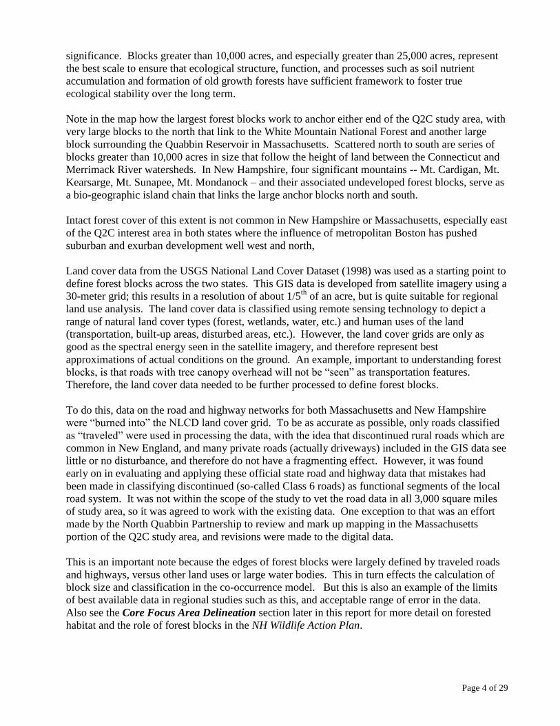
Important Forest Soils in Massachusetts

The soil groupings classification described above are unique

to New Hampshire, and do not exist in Massachusetts.

Therefore, an analysis was made of soils in the Massachusetts

portion of the Q2C to approximate the 1A, 1B, and 1C

groupings. Digital data for use in the GIS are not yet

available for Franklin County, so mapping and analysis in the

GIS were not possible; the missing data are evident in the

map to the right. A small amount of soils data are also

missing within the White Mountain National Forest at the

northern end of the Q2C region. Soils in adjacent New

Hampshire counties were used as a baseline for comparison

in Massachusetts counties since they most closely relate

across the state boundary. Where differing soil map units

were found state-to-state, the physical characteristics

described for N.H. soils was used to classify Massachusetts

soils using the N.H. system.

The map at right shows the extent and distribution of the

three most important forest soils in the Q2C region, and

which are discussed below.

Analysis

Of the soils mapped within the Q2C, approximately 573,000

acres (57%) are classed 1A, 350,000 acres (35%) are in group

1B, and 80,000 acres (8%) are 1C soils. This leaves about 973,000 acres (~50%) of the overall

Q2C region either unmapped, or distributed among less productive soils not considered in this

analysis.

As a check, in N.H. where the important forest soils groups are complete for most of the Q2C

region, about 60% of soils are 1A, 1B, or 1C, with approximately the same shares noted above for

soils mapped in this study. Therefore, somewhat less than 40% of soils are rated less productive,

allowing for the lack of soils data within the White Mountain National Forest in N.H. The same

ratios should apply in the Massachusetts portion of the Q2C if the Franklin County data were

available.

Page 7 of 29

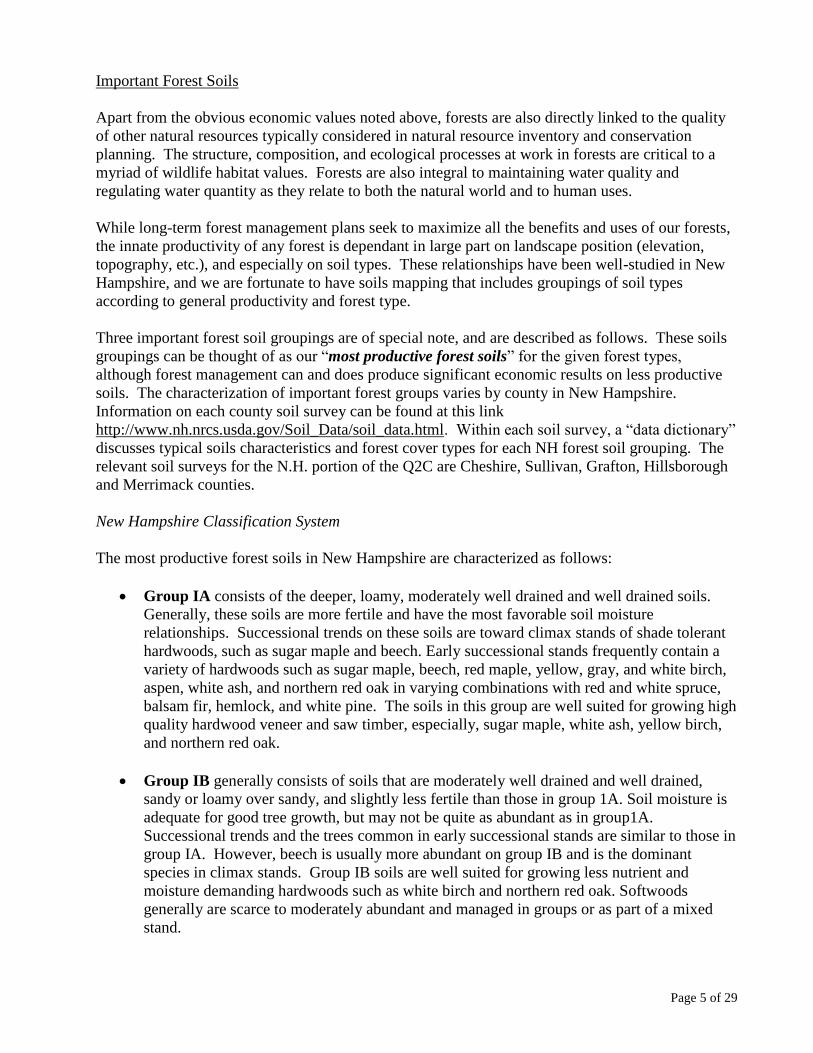
Important Agricultural Soils

The Farmland Protection Policy Act of 1981 was established to assure that Federal programs are

administered in a manner that will be compatible with state and local governments and private

programs and policies to protect farmland. The NRCS uses the following criteria in New

Hampshire for the purpose of carrying out the provisions of this Act.

Prime agricultural soils: interpreting from technical

soils data, prime agricultural soils have sufficient

available water capacity to produce the commonly

grown cultivated crops adapted to N.H., with high

nutrient availability, generally low slope and low

landscape position, not frequently flooded, and with

less than 10% rock fragments in the top six inches.

Corn fields and other row crops would be an example.

Soils of statewide importance: land that is not prime

but is considered farmland of statewide importance

for the production of food, feed, fiber, forage or

oilseed crops. Hay meadows not normally in row

cropping would be an example.

Soils of local importance: farmland that is not prime

or of statewide importance, but has local significance

for the production of food, feed, fiber and forage. In

The Q2C study area, this includes all land that is in

active farm use, but does not qualify as prime or of

statewide importance. Pasture land and hay meadows

would be examples.

For the purposes of the regional resource analysis in the Q2C interest area, only the first two

categories were included due to elevated importance for food and feed production activities typical

and important to agriculture in New England.

Prime agricultural and soils of statewide importance are classified uniformly in both Masschusetts

and New Hampshire, so no interpretation was made state-to-state. However, no soils data were

available digitally for Franklin County, as noted above.

It should be noted that no agricultural land use data were considered in this study, for two reasons.

First, with the exception of outdated land cover data from the USGS National Land Cover Dataset,

no uniform digital data are available across the two states. Second, using the soils data gives a

better sense of the potential for agricultural activity, versus actual land use which has been

decreasing significantly across New England for decades.1

1 See data in the USDS National Agricultural Statistical Survey available online at _______.

Page 8 of 29

Habitat Factors

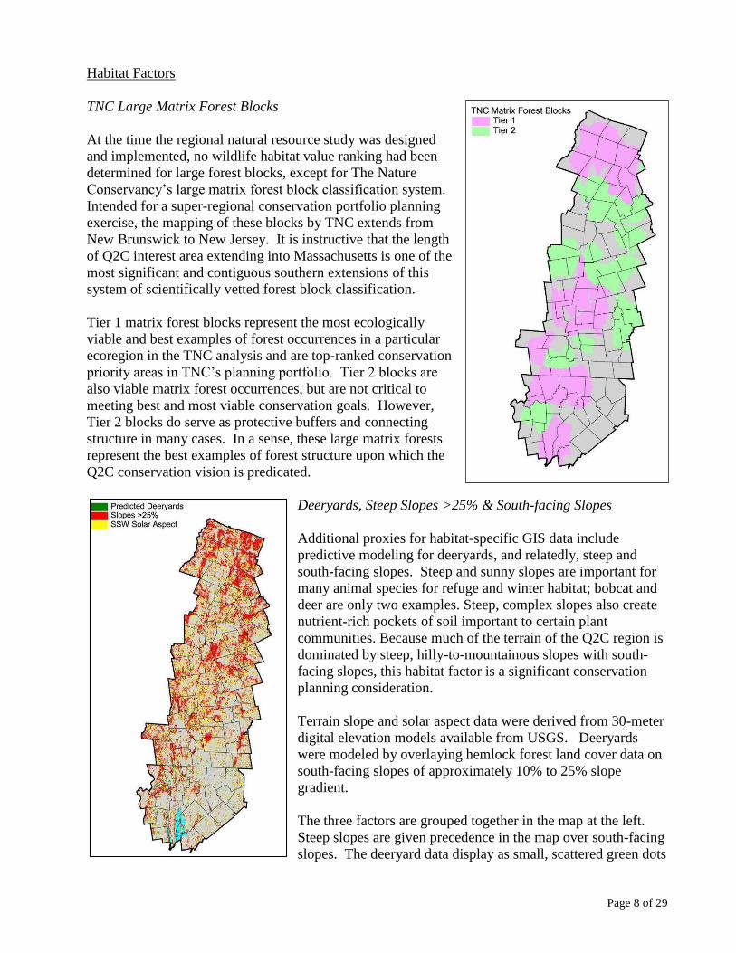
TNC Large Matrix Forest Blocks

At the time the regional natural resource study was designed

and implemented, no wildlife habitat value ranking had been

determined for large forest blocks, except for The Nature

Conservancy’s large matrix forest block classification system.

Intended for a super-regional conservation portfolio planning

exercise, the mapping of these blocks by TNC extends from

New Brunswick to New Jersey. It is instructive that the length

of Q2C interest area extending into Massachusetts is one of the

most significant and contiguous southern extensions of this

system of scientifically vetted forest block classification.

Tier 1 matrix forest blocks represent the most ecologically

viable and best examples of forest occurrences in a particular

ecoregion in the TNC analysis and are top-ranked conservation

priority areas in TNC’s planning portfolio. Tier 2 blocks are

also viable matrix forest occurrences, but are not critical to

meeting best and most viable conservation goals. However,

Tier 2 blocks do serve as protective buffers and connecting

structure in many cases. In a sense, these large matrix forests

represent the best examples of forest structure upon which the

Q2C conservation vision is predicated.

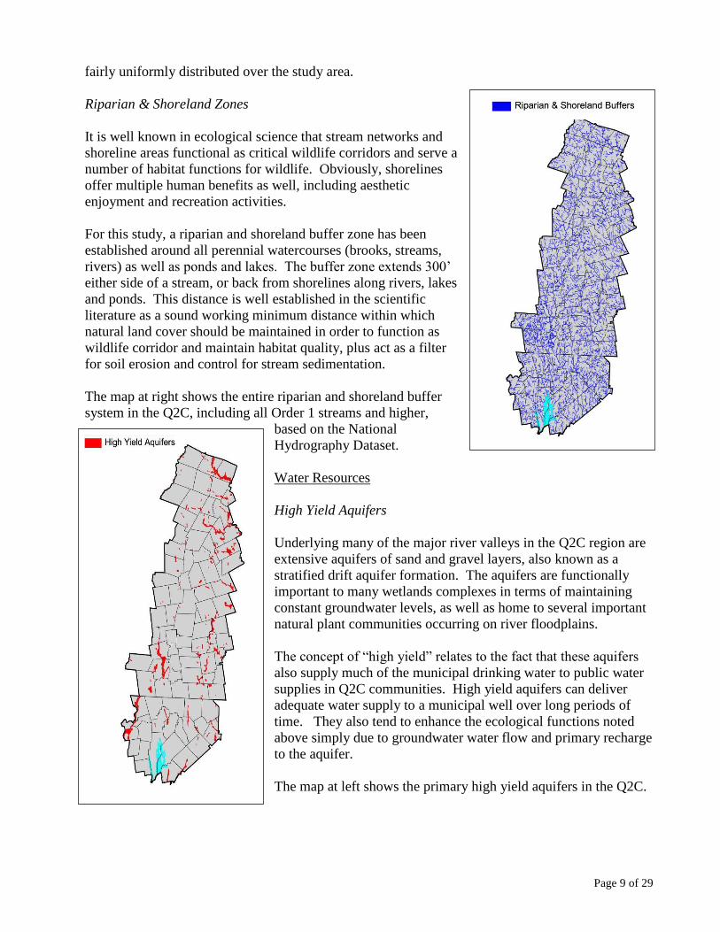
Deeryards, Steep Slopes >25% & South-facing Slopes

Additional proxies for habitat-specific GIS data include

predictive modeling for deeryards, and relatedly, steep and

south-facing slopes. Steep and sunny slopes are important for

many animal species for refuge and winter habitat; bobcat and

deer are only two examples. Steep, complex slopes also create

nutrient-rich pockets of soil important to certain plant

communities. Because much of the terrain of the Q2C region is

dominated by steep, hilly-to-mountainous slopes with south-

facing slopes, this habitat factor is a significant conservation

planning consideration.

Terrain slope and solar aspect data were derived from 30-meter

digital elevation models available from USGS. Deeryards

were modeled by overlaying hemlock forest land cover data on

south-facing slopes of approximately 10% to 25% slope

gradient.

The three factors are grouped together in the map at the left.

Steep slopes are given precedence in the map over south-facing

slopes. The deeryard data display as small, scattered green dots

Page 9 of 29

fairly uniformly distributed over the study area.

Riparian & Shoreland Zones

It is well known in ecological science that stream networks and

shoreline areas functional as critical wildlife corridors and serve a

number of habitat functions for wildlife. Obviously, shorelines

offer multiple human benefits as well, including aesthetic

enjoyment and recreation activities.

For this study, a riparian and shoreland buffer zone has been

established around all perennial watercourses (brooks, streams,

rivers) as well as ponds and lakes. The buffer zone extends 300’

either side of a stream, or back from shorelines along rivers, lakes

and ponds. This distance is well established in the scientific

literature as a sound working minimum distance within which

natural land cover should be maintained in order to function as

wildlife corridor and maintain habitat quality, plus act as a filter

for soil erosion and control for stream sedimentation.

The map at right shows the entire riparian and shoreland buffer

system in the Q2C, including all Order 1 streams and higher,

based on the National

Hydrography Dataset.

Water Resources

High Yield Aquifers

Underlying many of the major river valleys in the Q2C region are

extensive aquifers of sand and gravel layers, also known as a

stratified drift aquifer formation. The aquifers are functionally

important to many wetlands complexes in terms of maintaining

constant groundwater levels, as well as home to several important

natural plant communities occurring on river floodplains.

The concept of “high yield” relates to the fact that these aquifers

also supply much of the municipal drinking water to public water

supplies in Q2C communities. High yield aquifers can deliver

adequate water supply to a municipal well over long periods of

time. They also tend to enhance the ecological functions noted

above simply due to groundwater water flow and primary recharge

to the aquifer.

The map at left shows the primary high yield aquifers in the Q2C.

Page 10 of 29

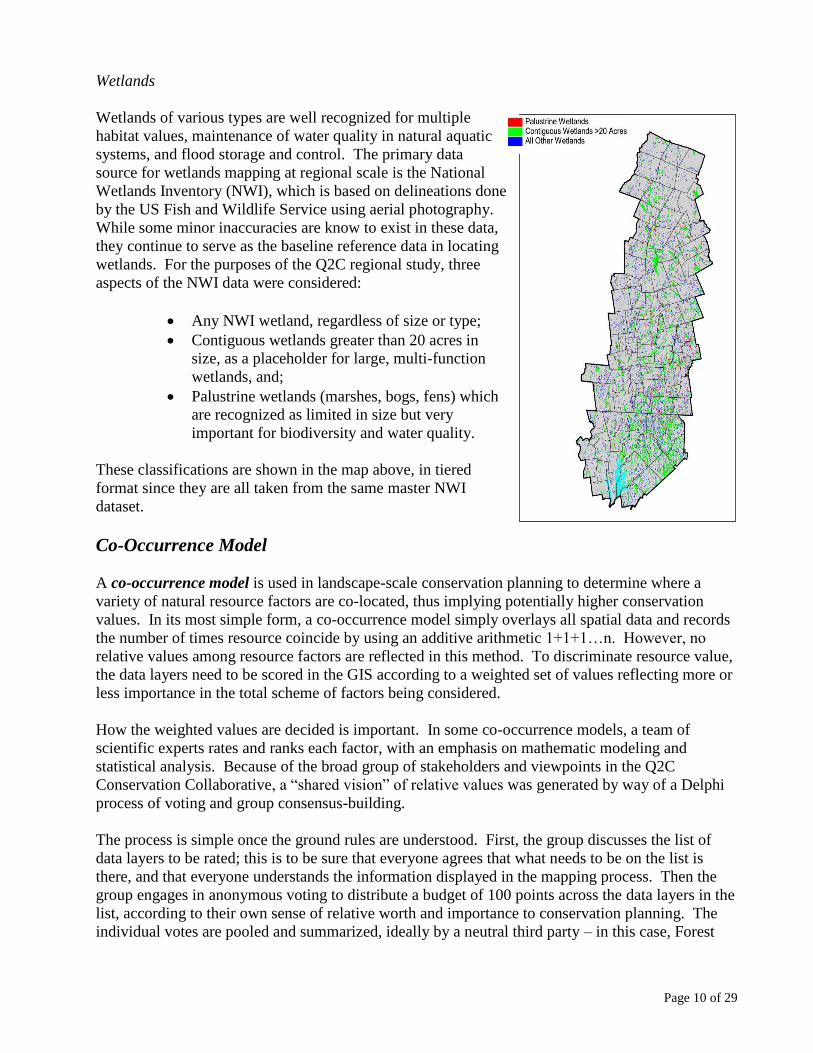
Wetlands

Wetlands of various types are well recognized for multiple

habitat values, maintenance of water quality in natural aquatic

systems, and flood storage and control. The primary data

source for wetlands mapping at regional scale is the National

Wetlands Inventory (NWI), which is based on delineations done

by the US Fish and Wildlife Service using aerial photography.

While some minor inaccuracies are know to exist in these data,

they continue to serve as the baseline reference data in locating

wetlands. For the purposes of the Q2C regional study, three

aspects of the NWI data were considered:

Any NWI wetland, regardless of size or type;

Contiguous wetlands greater than 20 acres in

size, as a placeholder for large, multi-function

wetlands, and;

Palustrine wetlands (marshes, bogs, fens) which

are recognized as limited in size but very

important for biodiversity and water quality.

These classifications are shown in the map above, in tiered

format since they are all taken from the same master NWI

dataset.

Co-Occurrence Model

A co-occurrence model is used in landscape-scale conservation planning to determine where a

variety of natural resource factors are co-located, thus implying potentially higher conservation

values. In its most simple form, a co-occurrence model simply overlays all spatial data and records

the number of times resource coincide by using an additive arithmetic 1+1+1…n. However, no

relative values among resource factors are reflected in this method. To discriminate resource value,

the data layers need to be scored in the GIS according to a weighted set of values reflecting more or

less importance in the total scheme of factors being considered.

How the weighted values are decided is important. In some co-occurrence models, a team of

scientific experts rates and ranks each factor, with an emphasis on mathematic modeling and

statistical analysis. Because of the broad group of stakeholders and viewpoints in the Q2C

Conservation Collaborative, a “shared vision” of relative values was generated by way of a Delphi

process of voting and group consensus-building.

The process is simple once the ground rules are understood. First, the group discusses the list of

data layers to be rated; this is to be sure that everyone agrees that what needs to be on the list is

there, and that everyone understands the information displayed in the mapping process. Then the

group engages in anonymous voting to distribute a budget of 100 points across the data layers in the

list, according to their own sense of relative worth and importance to conservation planning. The

individual votes are pooled and summarized, ideally by a neutral third party – in this case, Forest

Page 11 of 29

Society staff. A mean (average) value is calculated for each data layer, and fed into the GIS model

to produce a first-run co-occurrence map.

At this point, the group has an opportunity to review the anonymous vote/value range, along with

the map, and questions or comments can be posed that serve to clarify each person’s understanding

of the result of the first-round voting. The point of the anonymous voting is to eliminate the usual

group dynamic where the most skilled debater wins the point, so the results are not intended to be

debated. Each participant then has a second chance to vote, perhaps shifting points with better

understanding or changed viewpoint. With the Delphi process, consensus is usually reached in two

rounds of voting.

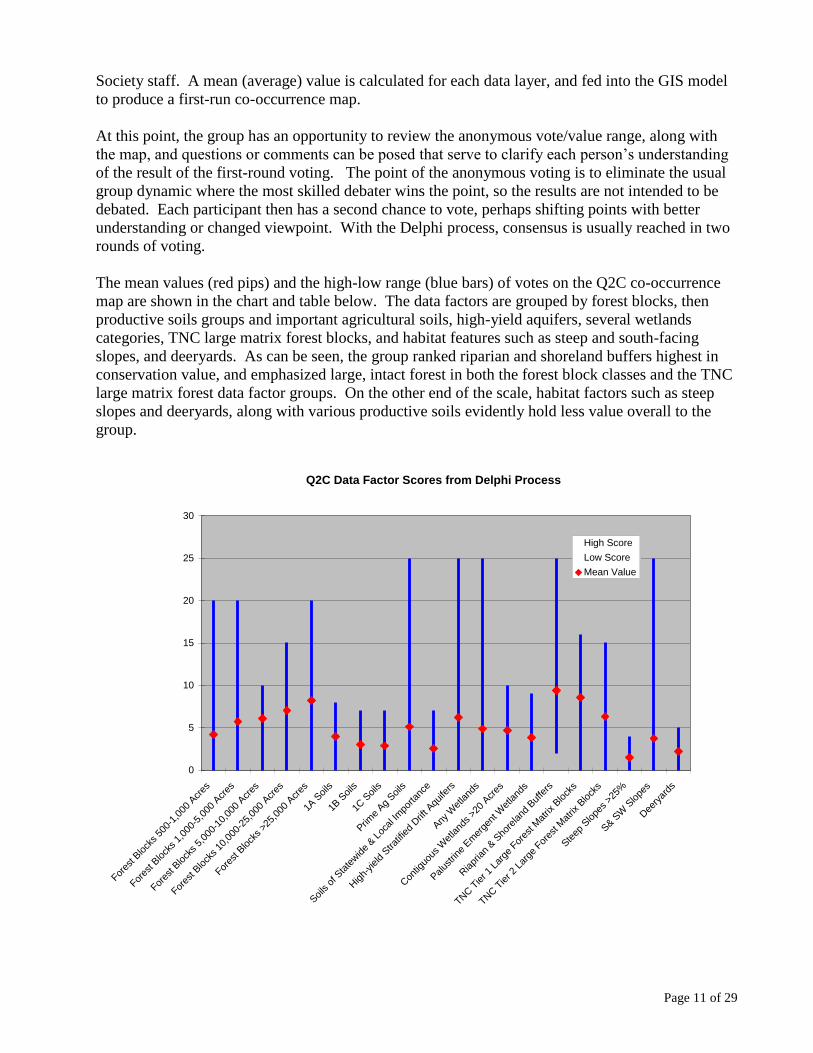
The mean values (red pips) and the high-low range (blue bars) of votes on the Q2C co-occurrence

map are shown in the chart and table below. The data factors are grouped by forest blocks, then

productive soils groups and important agricultural soils, high-yield aquifers, several wetlands

categories, TNC large matrix forest blocks, and habitat features such as steep and south-facing

slopes, and deeryards. As can be seen, the group ranked riparian and shoreland buffers highest in

conservation value, and emphasized large, intact forest in both the forest block classes and the TNC

large matrix forest data factor groups. On the other end of the scale, habitat factors such as steep

slopes and deeryards, along with various productive soils evidently hold less value overall to the

group.

Q2C Data Factor Scores from Delphi Process

0

5

10

15

20

25

30

Fores

t Block

s 50

0-1,

000

Acres

Fores

t Block

s 1,

000-

5,00

0 Acr

es

Fores

t Block

s 5,

000-

10,0

00 A

cres

Fores

t Block

s 10

,000

-25,

000

Acres

Fores

t Block

s >2

5,00

0 Acr

es

1A S

oils

1B S

oils

1C S

oils

Prim

e Ag

Soils

Soils o

f Sta

tewide

& Loc

al Im

porta

nce

High-

yield

Stra

tified

Drif

t Aqu

ifers

Any

Wet

land

s

Con

tiguo

us W

etland

s >2

0 Acr

es

Palus

trine

Em

erge

nt W

etland

s

Riapr

ian

& S

hore

land

Buf

fers

TNC T

ier 1

Lar

ge F

ores

t Mat

rix B

lock

s

TNC T

ier 2

Lar

ge F

ores

t Mat

rix B

lock

s

Ste

ep S

lope

s >2

5%

S& S

W S

lope

s

Dee

ryar

ds

High Score

Low Score

Mean Value

Page 12 of 29

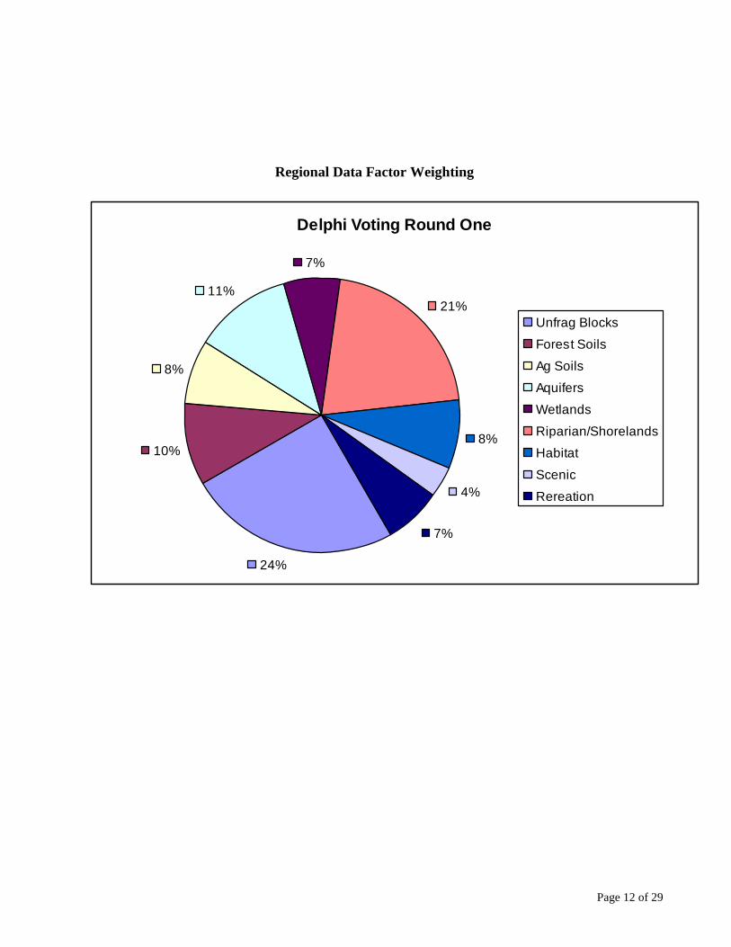
Regional Data Factor Weighting

Delphi Voting Round One

24%

10%

8%

11%

7%

21%

8%

4%

7%

Unfrag Blocks

Forest Soils

Ag Soils

Aquifers

Wetlands

Riparian/Shorelands

Habitat

Scenic

Rereation

Page 13 of 29

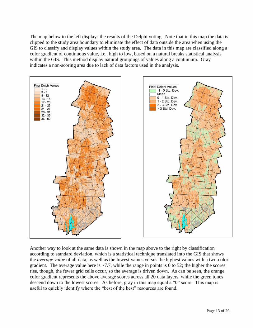
The map below to the left displays the results of the Delphi voting. Note that in this map the data is

clipped to the study area boundary to eliminate the effect of data outside the area when using the

GIS to classify and display values within the study area. The data in this map are classified along a

color gradient of continuous value, i.e., high to low, based on a natural breaks statistical analysis

within the GIS. This method display natural groupings of values along a continuum. Gray

indicates a non-scoring area due to lack of data factors used in the analysis.

Another way to look at the same data is shown in the map above to the right by classification

according to standard deviation, which is a statistical technique translated into the GIS that shows

the average value of all data, as well as the lowest values versus the highest values with a two-color

gradient. The average value here is ~7.7, while the range in points is 0 to 52; the higher the scores

rise, though, the fewer grid cells occur, so the average is driven down. As can be seen, the orange

color gradient represents the above average scores across all 20 data layers, while the green tones

descend down to the lowest scores. As before, gray in this map equal a “0” score. This map is

useful to quickly identify where the “best of the best” resources are found.

Page 14 of 29

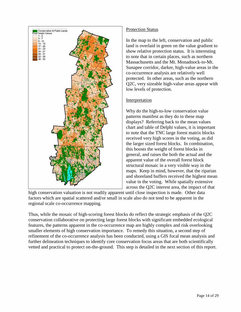
Protection Status

In the map to the left, conservation and public

land is overlaid in green on the value gradient to

show relative protection status. It is interesting

to note that in certain places, such as northern

Massachusetts and the Mt. Monadnock-to-Mt.

Sunapee corridor, darker, high-value areas in the

co-occurrence analysis are relatively well

protected. In other areas, such as the northern

Q2C, very sizeable high-value areas appear with

low levels of protection.

Interpretation

Why do the high-to-low conservation value

patterns manifest as they do in these map

displays? Referring back to the mean values

chart and table of Delphi values, it is important

to note that the TNC large forest matrix blocks

received very high scores in the voting, as did

the larger sized forest blocks. In combination,

this boosts the weight of forest blocks in

general, and raises the both the actual and the

apparent value of the overall forest block

structural mosaic in a very visible way in the

maps. Keep in mind, however, that the riparian

and shoreland buffers received the highest mean

value in the voting. While spatially extensive

across the Q2C interest area, the impact of that

high conservation valuation is not readily apparent until close inspection is made. Other data

factors which are spatial scattered and/or small in scale also do not tend to be apparent in the

regional scale co-occurrence mapping.

Thus, while the mosaic of high-scoring forest blocks do reflect the strategic emphasis of the Q2C

conservation collaborative on protecting large forest blocks with significant embedded ecological

features, the patterns apparent in the co-occurrence map are highly complex and risk overlooking

smaller elements of high conservation importance. To remedy this situation, a second step of

refinement of the co-occurrence analysis has been conducted, using a GIS focal mean analysis and

further delineation techniques to identify core conservation focus areas that are both scientifically

vetted and practical to protect on-the-ground. This step is detailed in the next section of this report.

Page 15 of 29

PHASE II -- Identifying Conservation Focus Areas, 2005-2006

The Quabbin to Cardigan Conservation Initiative strategic plan has been actively evolving for three

years. During 2005 and 2006, the regional planning process has been scaled down from its original

3,000 square mile extent, with the idea of a developing parcel-based conservation focus area (CFA)

for each of several generalized “core areas” identified by Q2C collaborators.

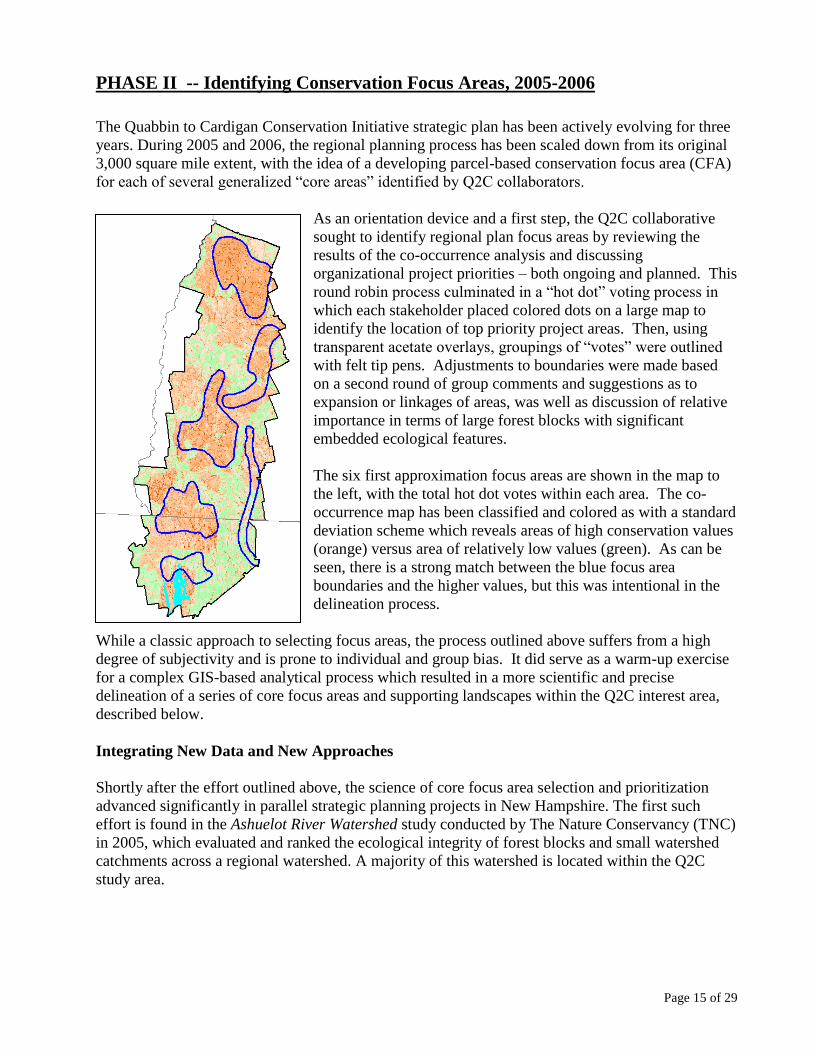
As an orientation device and a first step, the Q2C collaborative

sought to identify regional plan focus areas by reviewing the

results of the co-occurrence analysis and discussing

organizational project priorities – both ongoing and planned. This

round robin process culminated in a “hot dot” voting process in

which each stakeholder placed colored dots on a large map to

identify the location of top priority project areas. Then, using

transparent acetate overlays, groupings of “votes” were outlined

with felt tip pens. Adjustments to boundaries were made based

on a second round of group comments and suggestions as to

expansion or linkages of areas, was well as discussion of relative

importance in terms of large forest blocks with significant

embedded ecological features.

The six first approximation focus areas are shown in the map to

the left, with the total hot dot votes within each area. The co-

occurrence map has been classified and colored as with a standard

deviation scheme which reveals areas of high conservation values

(orange) versus area of relatively low values (green). As can be

seen, there is a strong match between the blue focus area

boundaries and the higher values, but this was intentional in the

delineation process.

While a classic approach to selecting focus areas, the process outlined above suffers from a high

degree of subjectivity and is prone to individual and group bias. It did serve as a warm-up exercise

for a complex GIS-based analytical process which resulted in a more scientific and precise

delineation of a series of core focus areas and supporting landscapes within the Q2C interest area,

described below.

Integrating New Data and New Approaches

Shortly after the effort outlined above, the science of core focus area selection and prioritization

advanced significantly in parallel strategic planning projects in New Hampshire. The first such

effort is found in the Ashuelot River Watershed study conducted by The Nature Conservancy (TNC)

in 2005, which evaluated and ranked the ecological integrity of forest blocks and small watershed

catchments across a regional watershed. A majority of this watershed is located within the Q2C

study area.

Page 16 of 29

The second, and perhaps more sophisticated approach to delineating core focus areas emerged from

the Coastal Watershed Land Conservation Plan, released in 2006; for more detail refer to

http://www.nhep.unh.edu/programs/community-assistance.htm#lcp

Working with regional resource co-occurrence mapping similar to that of the Q2C regional plan,

TNC and the Forest Society developed a more refined methodology

for the 1,000 square mile coastal watershed of New Hampshire.

That has now been replicated in the Q2C region, with some

modifications appropriate to the goals of the Q2C project, and the

particular resources addressed in the study (discussed below). In the

case of strategic conservation planning in the Q2C interest area,

taking a landscape-scale approach is imperative to the success of the

model. While incorporating local knowledge and town-wide data is

important when available, at this broad resolution it is not the main

focus of this exercise. Taking a “big picture” approach has resulted in

the most unbiased and meaningful results.

When the Q2C regional conservation planning project was first conceptualized, the available GIS

datasets were limited, especially in the realm of watershed-scale water quality data and wildlife

habitat. Since then, two significant additions have been added to the conservation planning toolkit:

the USGS SPARROW water quality model released in 2004, which generated very high

resolution watersheds for each stream catchment in New England, and characterized water

quality in each catchment; and,

the release of new ecologically-based wildlife data as part of the generation of Wildlife

Action Plans in both New Hampshire and Massachusetts.

Instead of revamping the entire regional study to accommodate the availability of new data in 2006,

the Q2C collaborative chose to build from the base of the strategic regional plan data developed to

date, starting with the Q2C co-occurrence mapping with its weighted resource values, and then

bringing in the WAP and SPARROW data as overlays and reference datasets. In this way, the

integrity of all preceding GIS planning work (and the investment in consensus-building) has been

preserved, while leaving open the option to incorporate “value-added” information from more

recent sources that reinforces the central goals and mission of the Q2C Partnerhsip.

Definitions

The following working definitions are offered as context in the following discussion. As indicated

above, we followed a similar methodology adapted from the recent Land Conservation Plan for

NH’s Coastal Watershed study, so these definitions are adapted from that plan.

Conservation Focus Area (CFA):

An area that is considered to be of exceptional significance for the protection of large forest blocks

with significant embedded ecological features (Q2C mission).

Core Area:

Page 17 of 29

A contiguous geographic area that contains a high concentration of natural resource values for

which the conservation focus area was identified, typically defined by major natural features such as

large forest blocks, near-pristine stream watersheds, and highest-ranked habitat features identified

by the NH Wildlife Action Plan.

Supporting Landscape:

The surrounding area that helps to safeguard the core area, typically composed of forest blocks

>1,000 acres, relatively high quality stream watersheds, and second rank WAP habitat features.

CFA Delineation Process

Focal Mean Analysis

As indicated above, we followed a targeting methodology adapted from the recent Land

Conservation Plan for NH’s Coastal Watershed involving feature-based delineation of conservation

focus areas. We first generated “statistical contouring” of the regional Q2C co-occurrence mapping,

using a focal mean GIS processing technique that averages scores within a moving analytical

window. This has the effect of smoothing the complex spatial mosaic of score variances in the

original co-occurrence map product by creating a continuous surface of relative values (it is

important to keep in mind that these are statistical values, not conservation values).

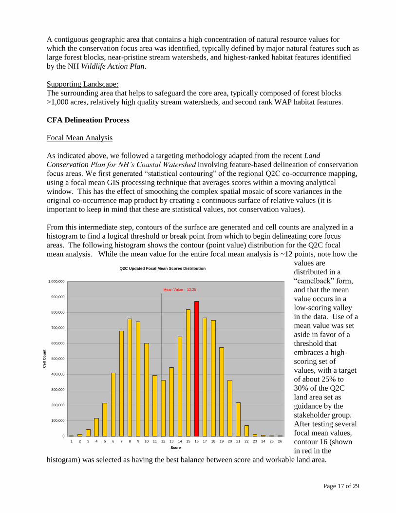
From this intermediate step, contours of the surface are generated and cell counts are analyzed in a

histogram to find a logical threshold or break point from which to begin delineating core focus

areas. The following histogram shows the contour (point value) distribution for the Q2C focal

mean analysis. While the mean value for the entire focal mean analysis is ~12 points, note how the

values are

distributed in a

“camelback” form,

and that the mean

value occurs in a

low-scoring valley

in the data. Use of a

mean value was set

aside in favor of a

threshold that

embraces a high-

scoring set of

values, with a target

of about 25% to

30% of the Q2C

land area set as

guidance by the

stakeholder group.

After testing several

focal mean values,

contour 16 (shown

in red in the

histogram) was selected as having the best balance between score and workable land area.

Q2C Updated Focal Mean Scores Distribution

0

100,000

200,000

300,000

400,000

500,000

600,000

700,000

800,000

900,000

1,000,000

1 2 3 4 5 6 7 8 9 10 11 12 13 14 15 16 17 18 19 20 21 22 23 24 25 26

Score

Ce

ll C

ou

nt

Mean Value = 12.25

Page 18 of 29

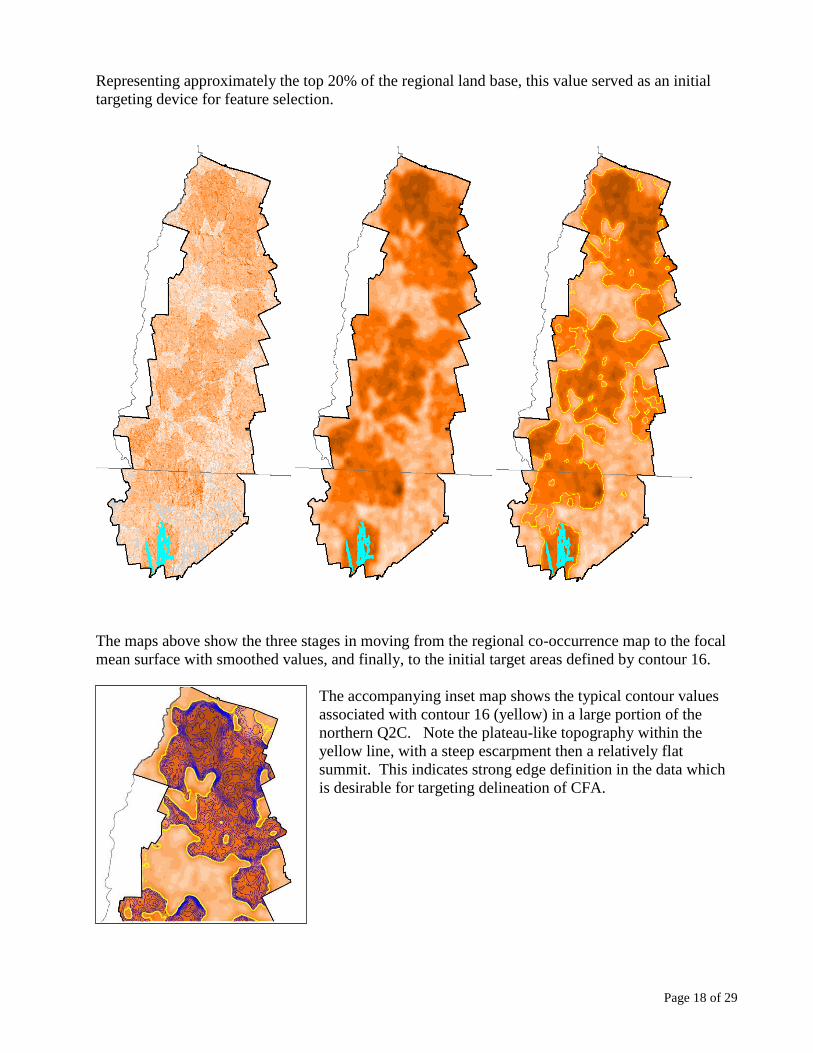
Representing approximately the top 20% of the regional land base, this value served as an initial

targeting device for feature selection.

The maps above show the three stages in moving from the regional co-occurrence map to the focal

mean surface with smoothed values, and finally, to the initial target areas defined by contour 16.

The accompanying inset map shows the typical contour values

associated with contour 16 (yellow) in a large portion of the

northern Q2C. Note the plateau-like topography within the

yellow line, with a steep escarpment then a relatively flat

summit. This indicates strong edge definition in the data which

is desirable for targeting delineation of CFA.

Page 19 of 29

Core Focus Area Structural Elements

The next step in the processing delineating CFA’s was to assemble key datasets in the GIS and

begin a process of comparing spatial relationships of key features in the landscape that would allow

real edges to be selected as CFA boundaries. These features need to be of relatively large size,

given the scale of the Q2C region, and important structural features in the scheme of natural

resource values being evaluated. This process was also used in the Coastal Plan, but again was

adapted for the scale and natural resource features evaluated in the Q2C interest area.

In New Hampshire:

Forest Blocks >1,000 acres (from TNC and NH WAP)

USGS SPARROW high quality stream watersheds

N.H. Fish and Game Wildlife Action Plan

N,H. Natural Heritage Bureau Element Occurrences Database

In Massachusetts:

TNC Roadless Forest Blocks

USGS SPARROW high quality stream watersheds

Outstanding Resource Waters data

Massachusetts Fisheries and Wildlife BioMap Project

(MA WAP)

The forest blocks data used in the CFA delineation represent

updated and upgraded block data compared to that available at

the time the regional co-occurrence model was run. This is

largely due to data acquisition and development generated for

the N.H. WAP. TNC worked with the N.H. Fish and Game

Department to refine forest block data using a newer dataset

(GRANIT land cover 2001) and a broader range of fragmenting

features, e.g., major transmission lines, railroads, etc.. Due to

the statewide scale of the WAP analysis and planning effort,

and the fact that habitat values increase typically with block

size, a minimum block size of 1,000 acres was used.

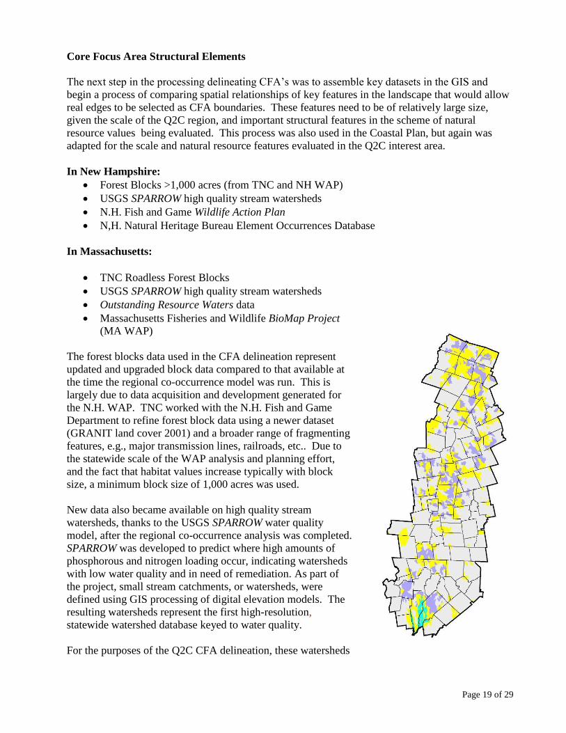
New data also became available on high quality stream

watersheds, thanks to the USGS SPARROW water quality

model, after the regional co-occurrence analysis was completed.

SPARROW was developed to predict where high amounts of

phosphorous and nitrogen loading occur, indicating watersheds

with low water quality and in need of remediation. As part of

the project, small stream catchments, or watersheds, were

defined using GIS processing of digital elevation models. The

resulting watersheds represent the first high-resolution,

statewide watershed database keyed to water quality.

For the purposes of the Q2C CFA delineation, these watersheds

Page 20 of 29

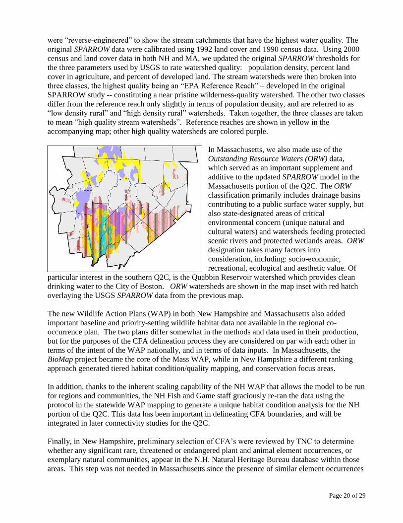
were “reverse-engineered” to show the stream catchments that have the highest water quality. The

original SPARROW data were calibrated using 1992 land cover and 1990 census data. Using 2000

census and land cover data in both NH and MA, we updated the original SPARROW thresholds for

the three parameters used by USGS to rate watershed quality: population density, percent land

cover in agriculture, and percent of developed land. The stream watersheds were then broken into

three classes, the highest quality being an “EPA Reference Reach” – developed in the original

SPARROW study -- constituting a near pristine wilderness-quality watershed. The other two classes

differ from the reference reach only slightly in terms of population density, and are referred to as

“low density rural” and “high density rural” watersheds. Taken together, the three classes are taken

to mean “high quality stream watersheds”. Reference reaches are shown in yellow in the

accompanying map; other high quality watersheds are colored purple.

In Massachusetts, we also made use of the

Outstanding Resource Waters (ORW) data,

which served as an important supplement and

additive to the updated SPARROW model in the

Massachusetts portion of the Q2C. The ORW

classification primarily includes drainage basins

contributing to a public surface water supply, but

also state-designated areas of critical

environmental concern (unique natural and

cultural waters) and watersheds feeding protected

scenic rivers and protected wetlands areas. ORW

designation takes many factors into

consideration, including: socio-economic,

recreational, ecological and aesthetic value. Of

particular interest in the southern Q2C, is the Quabbin Reservoir watershed which provides clean

drinking water to the City of Boston. ORW watersheds are shown in the map inset with red hatch

overlaying the USGS SPARROW data from the previous map.

The new Wildlife Action Plans (WAP) in both New Hampshire and Massachusetts also added

important baseline and priority-setting wildlife habitat data not available in the regional co-

occurrence plan. The two plans differ somewhat in the methods and data used in their production,

but for the purposes of the CFA delineation process they are considered on par with each other in

terms of the intent of the WAP nationally, and in terms of data inputs. In Massachusetts, the

BioMap project became the core of the Mass WAP, while in New Hampshire a different ranking

approach generated tiered habitat condition/quality mapping, and conservation focus areas.

In addition, thanks to the inherent scaling capability of the NH WAP that allows the model to be run

for regions and communities, the NH Fish and Game staff graciously re-ran the data using the

protocol in the statewide WAP mapping to generate a unique habitat condition analysis for the NH

portion of the Q2C. This data has been important in delineating CFA boundaries, and will be

integrated in later connectivity studies for the Q2C.

Finally, in New Hampshire, preliminary selection of CFA’s were reviewed by TNC to determine

whether any significant rare, threatened or endangered plant and animal element occurrences, or

exemplary natural communities, appear in the N.H. Natural Heritage Bureau database within those

areas. This step was not needed in Massachusetts since the presence of similar element occurrences

Page 21 of 29

had already been considered as part of the BioMap evaluation process. A similar review for special

habitat feature occurrences was made by the NH Fish and Game staff responsible for the WAP.

Delineation Decision Process

Background

Forest blocks and SPARROW watersheds that were contained or mostly contained within the 20%

threshold contour discussed above were selected as the basis for CFAs in the Q2C study area. The

areas where these two feature types overlapped created the basis for our core areas. Abutting forest

blocks and high quality watersheds that extended beyond the initial core areas were accounted for as

supporting landscapes.

The intersection of large roadless blocks with BioMap core areas and high quality watersheds

created the bulk of the foundation for the core areas in Massachusetts. BioMap data was found to be

highly precise, extensively ground-truthed, and of the appropriate level resolution for application.

After initial roughing out of CFA’s, three refinements added to the CFA delineation methodology

were implemented to finalize CFA boundaries:

The presence of NHB element occurrences that fall within forest blocks of any size

and that contribute to the greater system of CFA. In New Hampshire, this review

was conducted by The Natural Conservancy;

BioMap core areas and other known occurrences in Massachusetts; and,

Areas of special consideration that fall outside of the forest block thresholds, but

were deemed important in a review made by NH and MA Fish and Game

Departments, consistent with the NH WAP or the BioMap plan in Massachusetts.

Process Vignette

To more fully illustrate the decision model used in delineating CFA and supporting landscapes for

the Q2C region, the following series of map insets lay out the series of data factors used for the

northern portion of the Q2C study area. The first two maps represent the foundation data factors –

forest blocks and high quality stream watersheds -- followed by other important data sets that serve

to guide refinement of the CFA and supporting landscape boundaries. The final map points out

specific areas where a professional judgment was made in deciding the final outlines.

Contour 16 (the 20% factor) from the focal mean analysis is shown in the first few maps as the

starting point for CFA delineation. The later maps shift to the actual CFA boundary.

Page 22 of 29

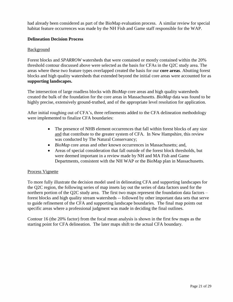
The map above shows the NH WAP forest blocks that intersect contour 16; these blocks form the

most basic structure of the CFA. The next map shows USGS SPARROW watersheds overlaid on

the forest blocks. Near pristine, EPA-defined reference reaches are shown in yellow, with

contiguous high quality rural stream watersheds in lavender. Taken together, these watersheds form

the core of the CFA where they overlap the forest blocks (see map on following page).

This map shows how the forest blocks and high

quality watershed combine to form CFA and

supporting landscapes, in green and lavender,

respectively. This first step in defining CFA then

moves onto secondary, qualitative considerations

that may cause adjustments to the preliminary

boundaries, typically reaching out to include

additional areas. This second step is outlined

below.

Page 23 of 29

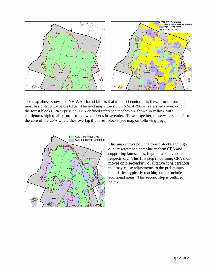
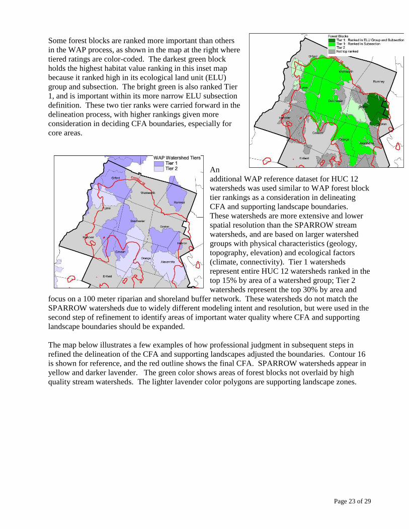
Some forest blocks are ranked more important than others

in the WAP process, as shown in the map at the right where

tiered ratings are color-coded. The darkest green block

holds the highest habitat value ranking in this inset map

because it ranked high in its ecological land unit (ELU)

group and subsection. The bright green is also ranked Tier

1, and is important within its more narrow ELU subsection

definition. These two tier ranks were carried forward in the

delineation process, with higher rankings given more

consideration in deciding CFA boundaries, especially for

core areas.

An

additional WAP reference dataset for HUC 12

watersheds was used similar to WAP forest block

tier rankings as a consideration in delineating

CFA and supporting landscape boundaries.

These watersheds are more extensive and lower

spatial resolution than the SPARROW stream

watersheds, and are based on larger watershed

groups with physical characteristics (geology,

topography, elevation) and ecological factors

(climate, connectivity). Tier 1 watersheds

represent entire HUC 12 watersheds ranked in the

top 15% by area of a watershed group; Tier 2

watersheds represent the top 30% by area and

focus on a 100 meter riparian and shoreland buffer network. These watersheds do not match the

SPARROW watersheds due to widely different modeling intent and resolution, but were used in the

second step of refinement to identify areas of important water quality where CFA and supporting

landscape boundaries should be expanded.

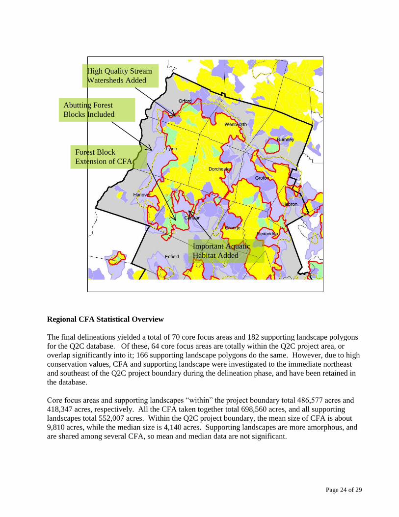
The map below illustrates a few examples of how professional judgment in subsequent steps in

refined the delineation of the CFA and supporting landscapes adjusted the boundaries. Contour 16

is shown for reference, and the red outline shows the final CFA. SPARROW watersheds appear in

yellow and darker lavender. The green color shows areas of forest blocks not overlaid by high

quality stream watersheds. The lighter lavender color polygons are supporting landscape zones.

Page 24 of 29

Forest Block

Extension of CFA

Important Aquatic

Habitat Added

High Quality Stream

Watersheds Added

Abutting Forest

Blocks Included

Regional CFA Statistical Overview

The final delineations yielded a total of 70 core focus areas and 182 supporting landscape polygons

for the Q2C database. Of these, 64 core focus areas are totally within the Q2C project area, or

overlap significantly into it; 166 supporting landscape polygons do the same. However, due to high

conservation values, CFA and supporting landscape were investigated to the immediate northeast

and southeast of the Q2C project boundary during the delineation phase, and have been retained in

the database.

Core focus areas and supporting landscapes “within” the project boundary total 486,577 acres and

418,347 acres, respectively. All the CFA taken together total 698,560 acres, and all supporting

landscapes total 552,007 acres. Within the Q2C project boundary, the mean size of CFA is about

9,810 acres, while the median size is 4,140 acres. Supporting landscapes are more amorphous, and

are shared among several CFA, so mean and median data are not significant.

Page 25 of 29

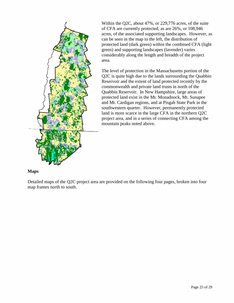
Within the Q2C, about 47%, or 229,776 acres, of the suite

of CFA are currently protected, as are 26%, or 108,946

acres, of the associated supporting landscapes. However, as

can be seen in the map to the left, the distribution of

protected land (dark green) within the combined CFA (light

green) and supporting landscapes (lavender) varies

considerably along the length and breadth of the project

area.

The level of protection in the Massachusetts portion of the

Q2C is quite high due to the lands surrounding the Quabbin

Reservoir and the extent of land protected recently by the

commonwealth and private land trusts in north of the

Quabbin Reservoir. In New Hampshire, large areas of

protected land exist in the Mt. Monadnock, Mt. Sunapee

and Mt. Cardigan regions, and at Pisgah State Park in the

southwestern quarter. However, permanently protected

land is more scarce in the large CFA in the northern Q2C

project area, and in a series of connecting CFA among the

mountain peaks noted above.

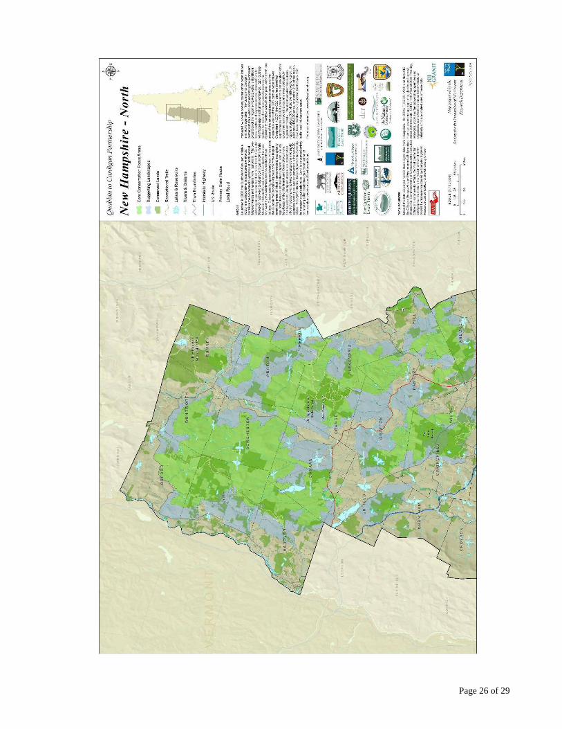
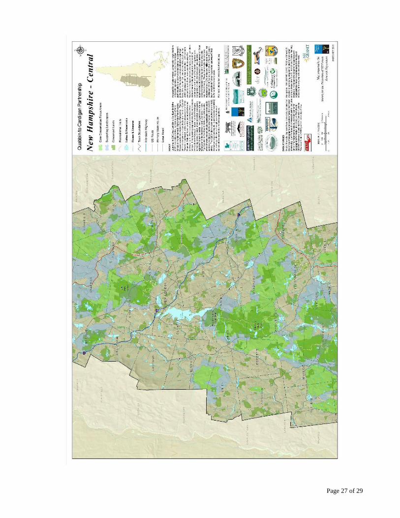
Maps

Detailed maps of the Q2C project area are provided on the following four pages, broken into four

map frames north to south.

Page 26 of 29

Page 27 of 29

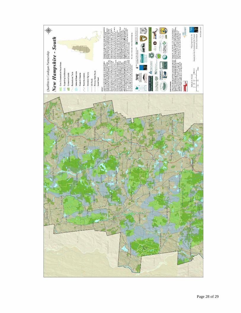
Page 28 of 29

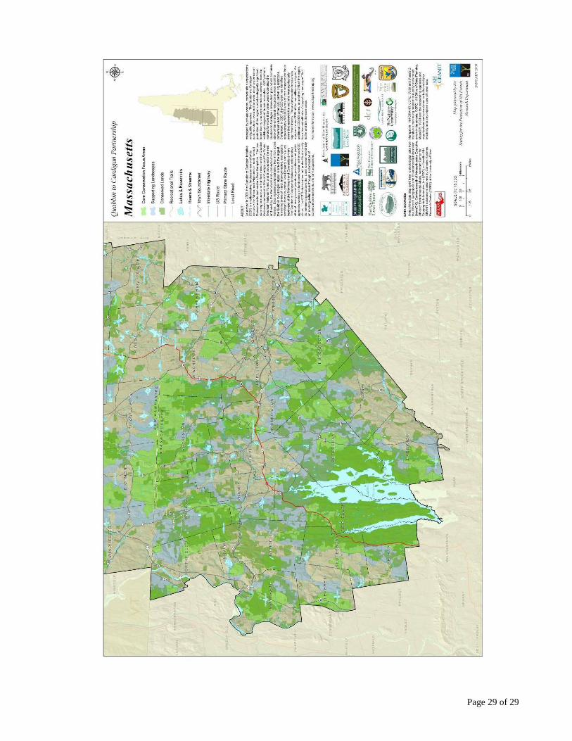
Page 29 of 29