Embed Size (px)
Citation preview

QUALITATIVE ANALYSIS OF ASOLOW MODEL ON TIME SCALES
MARTIN BOHNER, JULIUS HEIM AND AILIAN LIU
Abstract. In this paper, we further analyze the Solow model ontime scales. This model was recently introduced by the authorsand it combines the continuous and discrete Solow models and ex-tends them to different time scales. Assuming constant labor forcegrowth in the Solow model, we establish a comparison theorem.Then, under the more realistic assumption that the labor forcegrowth rate is a monotonically decreasing function, we discuss thecomparison theorem as well as stability and monotonicity of thesolutions of the Solow model. The economic meanings are alsoindicated in some remarks.
1. Introduction
The neoclassical growth model, developed by Solow [17] and Swan[18], had a great impact on how the economists think about economicgrowth. Since then, it has stimulated an enormous amount of work[2, 12, 20]. Since differential equation systems are usually more easilyhandled than difference systems from the analytical point of view, someof the economic models have used continuous timing [1,9,13–15] whileothers are given in difference models because some people think eco-nomic data are collected at discrete intervals and transformation of cap-ital into investments depends on the length of time lag, etc. [8, 10,21].
Hence, in economic modeling, either continuous timing or discretetiming is present, and there is not a common view among economistson which representation of time is better for economic models [14].Meanwhile, many results concerning differential equations may carryover quite easily to corresponding results for difference equations, whileother results seems to be completely different in nature from their con-tinuous counterparts [6].
2000 Mathematics Subject Classification. 91B62, 34C10, 39A10, 39A11, 39A12,39A13.
Key words and phrases. Solow model, time scales, labor growth rate, comparisonof solutions, stability.
1
183J. CONCRETE AND APPLICABLE MATHEMATICS, VOL. 13, NO.'S 3-4,183-197 ,2015, COPYRIGHT 2015 EUDOXUS PRESS LLC

2 MARTIN BOHNER, JULIUS HEIM AND AILIAN LIU
The blanket assumption that economic processes are either solelycontinuous or solely discrete, while convenient for traditional mathe-matical approaches, may sometimes be inappropriate, because in real-ity many economic phenomena do feature both continuous and discreteelements. In biology, a familiar example is a “seasonal breeding pop-ulation in which generations do not overlap” [6, 19]. A similar typicalexample in economics is the “seasonally changing investment and rev-enue in which seasons play an important effect on this kind of economicactivity”. In addition, option pricing and stock dynamics in finance [11]and the frequency and duration of market trading in economics [19] alsocontain this hybrid continuous-discrete processes.
Therefore, there is a great need to find a more flexible mathematicalframework to accurately model the dynamical blend of such systems, sothat they are precisely described and better understood. To meet thisrequirement, an emerging, progressive and modern area of mathemat-ics, known as “dynamic equations on time scales”, has been introduced.This calculus has the capacity to act as the framework to effectivelydescribe the above phenomena and to make advances in their associatefields, see e.g., [3–5,19].
This theory was introduced by Stefan Hilger in 1988 in his Ph.D.thesis [16] in order to unify continuous and discrete analysis, and hasbeen developed by many mathematicians. A time scale T is defined asany nonempty closed subset of R. In the time scales setting, once aresult is established, special cases include the result for the differentialequation when the time scale is the set of all real numbers R and theresult for the difference equation when the time scale is the set of allintegers Z. The induction principle plays an important role in theproofs of some of our results, so we give it here.
Theorem 1.1 (See [6, Theorem 1.7]). Let t0 ∈ T and assume that
{S(t) : t ∈ [t0,∞)}
is a family of statements satisfying:
A. The statement S(t0) is true.B. If t ∈ [t0,∞) is right-scattered and S(t) is true, then S(σ(t)) is
also true.C. If t ∈ [t0,∞) is right-dense and S(t) is true, then there is a neigh-
borhood U of t such that S(r) is true for all r ∈ U ∩ (t,∞).D. If t ∈ [t0,∞) is left-dense and S(r) is true for all r ∈ [t0, t), then
S(σ(t)) is true.
Then S(t) is true for all t ∈ [t0,∞).
184

QUALITATIVE ANALYSIS OF A SOLOW MODEL ON TIME SCALES 3
For other notations and a systematic introduction to time scalestheory, we refer the reader to [6, 7].
2. The Solow Model on Time Scales
In this section, we will first recall some elements of the Solow modelon general time scales as introduced by the authors in [5]. In the orig-inal Solow model [1,17], the key elements are the production function,i.e., how the inputs of capital K and labor L are transformed into out-puts, and how capital and labor force change over time. Here we stillassume the following:
1. The production function F satisfies:(a) F (λK, λL) = λF (K,L) for any λ,K,L ∈ R+ (constant return
to scales);(b) F (K, 0) = F (0, L) = 0 for any K,L ∈ R+;
(c)∂F
∂K> 0,
∂F
∂L> 0,
∂2F
∂K2< 0,
∂2F
∂L2< 0;
(d) limK→0+
∂F
∂K= lim
L→0+
∂F
∂L= ∞, lim
K→∞
∂F
∂K= lim
L→∞
∂F
∂L= 0 (Inada
conditions).2. The capital stock changes are equal to the gross investment I =sF (K,L) minus the capital depreciation δK, where s and δ are thesavings rate and the depreciation factor of goods, respectively.
3. The labor force L changes at a constant rate n.
The three assumptions give, for any t ∈ T
(2.1)
Y (t) = F (K(t), L(t)),
K∆(t) = I(t)− δK(t),
I(t) = sY (t),
L∆(t) = nL(t).
From (2.1), we obtain
(2.2) K∆(t) = sY (t)− δK(t) = sF (K(t), L(t))− δK(t).
Define
k(t) :=K(t)
L(t)and y(t) :=
Y (t)
L(t),
which are regarded as the capital stock per worker and the productionper worker, respectively. Let
f(k) := F
(K
L, 1
)= F (k, 1)
185
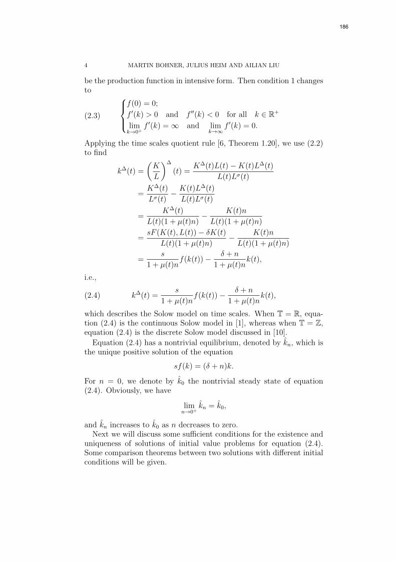
4 MARTIN BOHNER, JULIUS HEIM AND AILIAN LIU
be the production function in intensive form. Then condition 1 changesto
(2.3)
f(0) = 0;
f ′(k) > 0 and f ′′(k) < 0 for all k ∈ R+
limk→0+
f ′(k) =∞ and limk→∞
f ′(k) = 0.
Applying the time scales quotient rule [6, Theorem 1.20], we use (2.2)to find
k∆(t) =
(K
L
)∆
(t) =K∆(t)L(t)−K(t)L∆(t)
L(t)Lσ(t)
=K∆(t)
Lσ(t)− K(t)L∆(t)
L(t)Lσ(t)
=K∆(t)
L(t)(1 + µ(t)n)− K(t)n
L(t)(1 + µ(t)n)
=sF (K(t), L(t))− δK(t)
L(t)(1 + µ(t)n)− K(t)n
L(t)(1 + µ(t)n)
=s
1 + µ(t)nf(k(t))− δ + n
1 + µ(t)nk(t),
i.e.,
(2.4) k∆(t) =s
1 + µ(t)nf(k(t))− δ + n
1 + µ(t)nk(t),
which describes the Solow model on time scales. When T = R, equa-tion (2.4) is the continuous Solow model in [1], whereas when T = Z,equation (2.4) is the discrete Solow model discussed in [10].
Equation (2.4) has a nontrivial equilibrium, denoted by kn, which isthe unique positive solution of the equation
sf(k) = (δ + n)k.
For n = 0, we denote by k0 the nontrivial steady state of equation(2.4). Obviously, we have
limn→0+
kn = k0,
and kn increases to k0 as n decreases to zero.Next we will discuss some sufficient conditions for the existence and
uniqueness of solutions of initial value problems for equation (2.4).Some comparison theorems between two solutions with different initialconditions will be given.
186

QUALITATIVE ANALYSIS OF A SOLOW MODEL ON TIME SCALES 5
Theorem 2.1. Assume (2.3). For t0 ∈ T and k0 ∈ R+, the initialvalue problem
(2.5)
k∆(t) =s
1 + µ(t)nf(k(t))− δ + n
1 + µ(t)nk(t),
k(t0) = k0,
has a unique solution on T+t0
= {t ∈ T : t ≥ t0}.
Proof. Let
u(t, k) =s
1 + µ(t)nf(k)− δ + n
1 + µ(t)nk.
Then u(·, k) is rd-continuous and regressive on T, and
|u(t, k1)− u(t, k2)| =
∣∣∣∣∂u∂k (t, ξ)
∣∣∣∣ |k1 − k2|
=
∣∣∣∣ s
1 + µ(t)nf ′(ξ)− δ + n
1 + µ(t)n
∣∣∣∣ |k1 − k2|
≤ (sf ′(t0) + δ + n)|k1 − k2|,
where ξ ∈ (k1, k2). With the theorem of global existence and unique-ness in [6, Theorem 8.20], we can deduce that the solution of the prob-lem (2.5) exists uniquely. �
Hence in the following, with condition (2.3), we always have theexistence and uniqueness of solutions for initial value problems (2.5).
Theorem 2.2. Assume (2.3) and let δ > 0 be such that −δ ∈ R+. Letk1 and k2 be solutions of equation (2.4) on T+
t0with initial conditions
k1(t0) = k01 and k2(t0) = k02, respectively. If 0 < k01 < k02, then
k1 < k2 on T+t0.
Proof. We use the induction principle Theorem 1.1.
A. If t = t0, then the result is obvious from the hypothesis.B. If t ∈ T+
t0is right-scattered and k1(t) < k2(t), then
k1(σ(t))− k2(σ(t)) = k1(t)− k2(t) + µ(t)(k∆1 (t)− k∆
2 (t))
= k1(t)− k2(t) +µ(t)
1 + µ(t)n[sf(k1(t))− (δ + n)k1(t)]
− µ(t)
1 + µ(t)n[sf(k2(t))− (δ + n)k2(t)]
= k1(t)− k2(t) +sµ(t)
1 + µ(t)n[f(k1(t))− f(k2(t))]
187

6 MARTIN BOHNER, JULIUS HEIM AND AILIAN LIU
−(δ + n)µ(t)
1 + µ(t)n[k1(t)− k2(t)]
=1− µ(t)δ
1 + µ(t)n[k1(t)− k2(t)] +
µ(t)s
1 + µ(t)n[f(k1(t))− f(k2(t))]
< 0,
so
k1(σ(t)) < k2(σ(t)).
C. If t is right-dense and k1(t) < k2(t), then there exists a right neigh-
borhood U+(t)∩T of t such that k1(r) < k2(r) for any r ∈ U+(t)∩T.For if such a neighborhood does not exist, then there must exist adecreasing series {tn} ⊂ U+(t) ∩ T and lim
n→∞tn = t, such that
k1(tn) ≥ k2(tn)
and taking limit on both sides, we obtain k1(t) ≥ k2(t), a contra-diction.
D. If t is left-dense and k1(r) < k2(r) for any r ∈ [t0, t) ∩ T, thenfrom the continuity of the solutions, k1(t) ≤ k2(t). Uniqueness ofsolutions of initial value problems yields k1(t) < k2(t).
Now an application of Theorem 1.1 concludes the proof. �
Note that Theorem 2.2 implies that the solution for the initial valueproblem (2.5) is always positive provided k(t0) > 0.
Corollary 2.3. Assume (2.3) and let δ > 0 be such that −δ ∈ R+.Then all solutions of equation (2.4) converge to the nontrivial steady
state kn monotonically, and the equilibrium point kn is asymptoticallystable and hence is a global attractor.
Proof. If k(t0) < kn, then Theorem 2.2 implies that
k(t) < kn for any t ∈ T+t0.
Hence
k∆(t) =s
1 + µ(t)nf(k(t))− δ + n
1 + µ(t)nk(t) > 0 for any t ∈ T+
t0.
This means that k is increasing to the equilibrium point. Similar argu-ments apply to the case with k(t0) > kn, which concludes the proof. �
Remark 2.4. Corollary 2.3 means that for two countries or districts withconstant population growth rates, the one with the smaller populationgrowth rate has a bigger capital per worker in the long run.
188

QUALITATIVE ANALYSIS OF A SOLOW MODEL ON TIME SCALES 7
3. Improved Solow Model on Time Scales
In Section 2, we assumed that the labor force L grows at a constantrate n on the time scale, i.e.,
(3.1) L∆(t) = nL(t),
which implies that the labor force grows exponentially, that is,
L(t) = L0en(t, t0),
where L0 is the initial labor level at t0 ∈ T. With the properties of theexponential function on time scales and the fact that n > 0, we have
limt→∞
L(t) =∞.
This means the labor force approaches infinity when t goes to infinity,which is unrealistic, because in reality the environment has a carryingcapacity. So the simple growth model of labor in equation (3.1) canprovide an adequate approximation to such growth only for an initialperiod, but does not accommodate growth reductions due to competi-tion for environmental resources such as food, habitat and the policyfactor etc. [1].
Since the 1950s, developing countries have recognized that the highpopulation growth rate has seriously hampered the economic growthand adopted the population control policy. As a result, the populationgrowth rates of many countries decreased fast in the last 40 years, suchas in China. Also due to the aging of the population and, consequently,a dramatic increase in the number of deaths, the population growth ratedecreased below zero in some developed countries, and is projected todecrease to zero during the next few decades in the developing countries[1].
So to incorporate the numerical upper bound on the growth size, onthe reference of [10], we revise Condition 3 from Section 2 as follows.
3.′ The labor force L satisfies the following properties:(a) The population is strictly increasing and bounded, i.e.,
L > 0, L∆ > 0 on T+t0
and limt→∞
L(t) = L∞ <∞.
(b) The population growth rate is decreasing to 0, i.e.,
If n =L∆
L, then lim
t→∞n(t) = 0 and n∆ < 0 on T+
t0.
Hence equation (2.4) takes the form
(3.2) k∆(t) =s
1 + µ(t)n(t)f(k(t))− δ + n(t)
1 + µ(t)n(t)k(t).
189

8 MARTIN BOHNER, JULIUS HEIM AND AILIAN LIU
Note that this is a nonautonomous dynamic equation on a time scale.Next we give the theorem of existence and uniqueness for solutions ofinitial value problems for (3.2).
Theorem 3.1. Assume (2.3). For t0 ∈ T and k0 ∈ R+, the initialvalue problem
(3.3)
k∆(t) =s
1 + µ(t)n(t)f(k(t))− δ + n(t)
1 + µ(t)n(t)k(t)
k(t0) = k0,
has a unique solution on T+t0.
Proof. Following the same way as in the proof of Theorem 2.1, we let
u(t, k) =s
1 + µ(t)n(t)f(k)− δ + n(t)
1 + µ(t)n(t)k.
So u(·, k) is rd-continuous and regressive, and∣∣∣∣∂u∂k (t, ξ)
∣∣∣∣ ≤ sf ′(k0) + δ + n(t0).
From the theorem of global existence and uniqueness in [6], the solutionof the problem (3.3) exists uniquely. �
Theorem 3.2. Assume (2.3) and let δ > 0 be such that −δ ∈ R+. Letk1 and k2 be solutions of equation (3.2) with initial conditions k1(t0) =k01 and k2(t0) = k02, respectively. If 0 < k01 < k02, then
k1 < k2 on T+t0.
Proof. The proof is similar to the proof of Theorem 2.2. �
Remark 3.3. Theorem 3.2 means that if two economies have the samefundamentals, then the one with the bigger initial capital per workerwill always have the bigger capital per worker for ever on any timescale. The result in Theorem 3.2 includes the results in [1] and [10] asspecial cases.
Theorem 3.4. Assume (2.3) and let δ > 0 be such that −δ ∈ R+. Letk1 and k2 be solutions of the dynamic equations on the same time scale
(3.4) k∆(t) =s
1 + µ(t)n1(t)f(k(t))− δ + n1(t)
1 + µ(t)n1(t)k(t) =: u(k(t), t)
and
(3.5) k∆(t) =s
1 + µ(t)n2(t)f(k(t))− δ + n2(t)
1 + µ(t)n2(t)k(t) =: v(k(t), t),
190

QUALITATIVE ANALYSIS OF A SOLOW MODEL ON TIME SCALES 9
respectively, with the same initial condition k1(t0) = k2(t0). If n1 < n2
on T+t0, then
k1 ≥ k2 on T+t0.
Proof. From n1(t) < n2(t), we have u(k(t), t) > v(k(t), t) for all t ∈ T+t0
.Let z := k1 − k2. Obviously, we have z(t0) = k1(t0)− k2(t0) = 0 and
z∆(t0) = k∆1 (t0)− k∆
2 (t0) = u(k1(t0), t0)− v(k2(t0), t0) > 0.
So z is right-increasing at t0, i.e., if t0 is right-scattered, then we havez(σ(t0)) > z(t0) = 0; if t0 is right-dense, then there exists a nonempty
neighborhood U+(t0)∩T of t0 such that z(t) > 0 for any t ∈ U+(t0)∩T.We now show that z ≥ 0 holds on T+
t0. If this is not the case, then
there must be a point t1 > t0, t1 ∈ T such that z(t1) < 0 and z(t) ≥ 0when t ∈ (t0, t1) ∩ T. If t1 is left-dense, then continuity of z gives thatz(t1) ≥ 0, which contradicts the assumption. Hence t1 is left-scattered.Let ρ(t1) = t2. Then z(t2) ≥ 0, i.e., k1(t2) ≥ k2(t2). Let k′2 be thesolution of equation (3.5) satisfying the initial condition k′2(t2) = k1(t2).From the discussion in the beginning of this proof, we obtain that k1−k′2is also right-increasing at t2, i.e.,
(3.6) k1(t) > k′2(t) for t ∈ U+(t2) ∩ T,
where U+(t2) ∩ T is a nonempty right neighborhood of t2 (at leastincluding t1). Taking into account that k2(t2) ≤ k′2(t2), Theorem 3.2gives
(3.7) k2(t) ≤ k′2(t) for all t ∈ T+t2.
From (3.6) and (3.7), we have
k1(t) > k2(t) for t ∈ U+(t2) ∩ T,
and thus k1(t1) > k2(t1), which contradicts the fact z(t1) < 0. Thisconcludes the proof. �
Remark 3.5. Theorem 3.4 implies that, on any economic domain, fortwo economies with the same initial capital per worker, the economywith the smaller population growth rate will always have the biggercapital per worker on any time scale. The result here also includes theresults in [1, 13] and [10] as special cases.
Theorem 3.6. Assume (2.3) and let δ > 0 be such that −δ ∈ R+. If
k solves (3.2), then limt→∞
k(t) = k0.
191

10 MARTIN BOHNER, JULIUS HEIM AND AILIAN LIU
Proof. We want to prove that for any ε > 0, there exists T > 0, suchthat if t > T , t ∈ T, we have |k(t)− k0| < ε. Now let ε > 0. Since
limn→0+
kn = k0,
we know that there exists n > 0 such that
|kn − k0| <ε
3for all n ∈ (0, n).
Let t1 ∈ T+t0
such that nt1 = n(t1) < n, i and let knt1and k0 be the
solutions of
k∆(t) =s
1 + µ(t)nt1f(k(t))− δ + nt1
1 + µ(t)nt1k(t)
andk∆(t) = sf(k(t))− δk(t),
respectively, with the initial conditions
knt1(t1) = k0(t1) = k(t1).
Then Theorem 3.4 implies that
knt1(t) ≤ k(t) ≤ k0(t) for all t ∈ T+
t1.
Since limt→∞
k0(t) = k0, there exists T1 > 0 such that
|k0(t)− k0| <ε
3for all t > T1.
Moreover, since limt→∞
knt1(t) = knt1
, there exists T2 > 0 such that
|knt1(t)− knt1
| < ε
3for all t > T2.
Hence for t > T := max{T1, T2, t1}, we have
k0 −2
3ε < knt1
− ε
3< knt1
(t) ≤ k(t) ≤ k0(t) < k0 +ε
3,
which implies that |k(t)− k0| < ε for any t ∈ T+T . �
Remark 3.7. Theorem 3.6 says that for any economic domain T, thepopulation growth rate n(t) has no influence on the level of per workeroutput in the long run. That is, provided that the economy possessesa population growth rate strictly decreasing to zero, the capital perworker always converges to the positive steady state of the Solow modelon a time scale with a population growth rate of zero.
Theorem 3.8. Assume (2.3) and let δ > 0 be such that −δ ∈ R+.Then the solution k of (3.2) with k(t0) = k0 is asymptotically stable.
192

QUALITATIVE ANALYSIS OF A SOLOW MODEL ON TIME SCALES 11
Proof. To prove the Lyapunov stability of k in equation (3.2) withinitial condition k(t0) = k0, we have to show that for any ε > 0, thereexists η > 0 such that for any solution q of equation (3.2) with initialcondition q(t0) = q0 and such that |k(t0)− q(t0)| < η, we have
|k(t)− q(t)| < ε for any t ∈ T+t0.
Let ϕ1 and ϕ2 be the solutions of equation (3.2) with initial conditions
ϕ1(t0) =3
2k(t0) and ϕ2(t0) =
1
2k(t0), respectively. From Theorem 3.6,
we have
limt→∞
ϕ1(t) = limt→∞
ϕ2(t) = k0 = limt→∞
k(t).
Thus, for any ε > 0, there exists t1 > t0, t1 ∈ T+t0
, such that
|ϕ1(t)− k(t)| < ε
2and |ϕ2(t)− k(t)| < ε
2for all t ∈ T+
t1.
Let q solve (3.2) with the initial condition q0 ∈(
1
2k(t0),
3
2k(t0)
). From
Theorem 3.2, we have
ϕ1(t) < q(t) < ϕ2(t) for any t ∈ T+t0.
Thus
|q(t)− k(t)| < ε for any t ∈ T+t1.
Next we choose η such that for any solution q with initial value q0,|q0 − k0| < η implies |k − q| < ε on [t0, t1] ∩ T. Following the proofof the theorem of continuous dependence on initial conditions, makinguse of the finite covering theorem, we can obtain that for any ε > 0,there exists η < k0/2 such that |q0 − k0| < η implies |k(t) − q(t)| < εfor all t ∈ [t0, t1] ∩ T. From Theorem 3.6, for any solutions k and q ofequation (3.2), we have that
limt→∞
k(t) = limt→∞
q(t) = k0,
and then
limt→∞|q(t)− k(t)| = 0.
So the solution of equation (3.2) is asymptotically stable. �
Remark 3.9. Theorem 3.8 says that under the same fundamentals, iftwo economies operating on the same time domain have nearly thesame initial capital per worker, the following capitals per worker willtake on similar behavior.
Next we will present the monotonicity of the solutions of (3.2).
193

12 MARTIN BOHNER, JULIUS HEIM AND AILIAN LIU
Theorem 3.10. Assume (2.3) and let δ > 0 be such that −δ ∈ R+.Let t0 ∈ T and k, knt0
, k0 be solutions of the dynamic equation (3.2),
(3.8) k∆(t) =s
1 + µ(t0)nt0f(k(t))− δ + nt0
1 + µ(t0)nt0k(t),
and
(3.9) k∆(t) = sf(k(t))− δk(t),
respectively, with the initial values
k(t0) = knt0(t0) = k0(t0).
Then
1. knt0≤ k ≤ k0 on T+
t0;
2. If k(t0) ≤ kn0, then k is strictly increasing on T+t0;
3. If kn0 < k(t0) ≤ k0, then there exists t ∈ T such that k is decreasingon [t0, t] ∩ T and is increasing on T+
t;
4. If k0 < k(t0), then k is increasing on T+t0, or there exists t ∈ T
such that k is decreasing on [t0, t] ∩ T and is increasing on T+
t.
Here kn0 and k0 are the equilibria of (3.8) and (3.9), respectively.
Proof. 1. For t > t0, t ∈ T, we have n(t0) > n(t) > 0. So fromTheorem 3.4, we obtain the result easily.
2. We want to prove the statement S(t) given by k∆(t) > 0 is truefor any t ∈ T+
t0. To do this, we use Theorem 1.1.
A. Since k(t0) < kn0 , we have k∆(t0) > 0. So S(t) holds at t = t0.B. If t is right-scattered and k∆(t) > 0, then
k(σ(t)) = k(t) + µ(t)k∆(t)
= k(t) + µ(t)sf(k(t))− (δ + n(t))k(t)
1 + µ(t)n(t)
=(1− µ(t)δ)k(t) + sµ(t)f(k(t))
1 + µ(t)n(t)
<(1− µ(t)δ)k(σ(t)) + sµ(t)f(k(σ(t)))
1 + µ(t)n(σ(t))
=[1 + µ(t)n(σ(t))]k(σ(t))
1 + µ(t)n(σ(t))
+µ(t)[sf(k(σ(t)))− (δ + n(σ(t)))k(σ(t))]
1 + µ(t)n(σ(t))
= k(σ(t)) +µ(t)
1 + µ(t)n(σ(t))[1 + µ(σ(t))n(σ(t))]k∆(σ(t)),
194

QUALITATIVE ANALYSIS OF A SOLOW MODEL ON TIME SCALES 13
so k∆(σ(t)) > 0.C. If t is right-dense and k∆(t) > 0, then there exists a neighbor-
hood U+(t) ∩ T such that k∆(r) > 0 for any r ∈ U+(t) ∩ T.To prove this, we assume that there does not exist such aneighborhood. Then there must exist a decreasing sequence{tn} ⊂ U+(t) ∩ T such that lim
n→∞tn = t and k∆(tn) ≤ 0.
From the properties of f , taking limit on both sides, we obtaink∆(t) ≤ 0, which is a contradiction.
D. Assume that t is left-dense and k∆(r) > 0 for any r ∈ [t0, t)∩T.From continuity, we can get k∆(t) ≥ 0. If k∆(t) = 0, then forany r ∈ [t0, t) ∩ T, from the chain rule in [6], we have
[(1 + µn)k∆]∆(r) = [s(f ◦ k)− (δ + n)k]∆(r)
= sf ′(k(r))k∆(r)− n∆(r)k(r)
−(δ + nσ(r))k∆(r).
Taking limit on both sides when r → t−, we obtain
[(1 + µn)k∆)]∆(t) = −n∆(t)k(t) > 0.
So since t is left-dense and from the continuity, we have
(1 + µ(t)n(t))k∆(t) > (1 + µ(r)n(r))k∆(r) > 0
for all r ∈ U−(t) ∩ T. Hence k∆(t) > 0.
3. If kn0 < k(t0) ≤ k0, then
k∆(t0) =s
1 + µ(t0)n(t0)f(k(t0))− δ + n(t0)
1 + µ(t0)n(t0)k(t0)
=s
1 + µ(t0)n(t0)f(knt0
(t0))− δ + n(t0)
1 + µ(t0)n(t0)knt0
(t0)
= k∆nt0
(t0) < 0.
Hence k is right-decreasing at t0, i.e., if t0 is right-scattered, thenk(σ(t0)) < k(t0); if t0 is right-dense, then there exists a nonempty
neighborhood U+(t0) ∩ T of t0 such that k(t) < k(t0) for any t ∈U+(t0) ∩ T. If k∆ ≤ 0 is true on T+
t0, then k is decreasing on T+
t0.
Considering limt→∞
k(t) = k0 in Theorem 3.6, we have
k0 ≤ k(t) < k(t0) ≤ k0 for t ∈ T+t0,
which is a contradiction. So there must exist t ∈ T+t0
such that
k∆(t) > 0, and for simplicity we assume t is the first point thatverifies the inequality. So it must be proved that k∆(t) > 0 for allt ∈ T+
t, which is similar to the proof of Statement 2.
195

14 MARTIN BOHNER, JULIUS HEIM AND AILIAN LIU
4. Following the same proof as in Statement 3, we can obtain themonotonicity.
This completes the proof. �
Acknowledgements
This work was financially supported by Grants ZR2012AQ024 andZR2010AL014 from NSF of Shandong Province.
References
[1] Elvio Accinelli and Juan Gabriel Brida. Population growth and the Solow-Swanmodel. Int. J. Ecol. Econ. Stat., 8(S07):54–63, 2007.
[2] Robert J. Barro and Xavier Sala-i Martin. Economic Growth. McGraw-Hill,Inc., 1994.
[3] Martin Bohner and Gregory Gelles. Risk aversion and risk vulnerability inthe continuous and discrete case. A unified treatment with extensions. Decis.Econ. Finance, 35:1–28, 2012.
[4] Martin Bohner, Gregory Gelles, and Julius Heim. Multiplier-accelerator mod-els on time scales. Int. J. Stat. Econ., 4(S10):1–12, 2010.
[5] Martin Bohner, Julius Heim, and Ailian Liu. Solow models on time scales.Cubo, 15(1):13–32, 2013.
[6] Martin Bohner and Allan Peterson. Dynamic equations on time scales: anintroduction with applications. Birkhauser Boston Inc., Boston, MA, 2001.
[7] Martin Bohner and Allan Peterson. Advances in dynamic equations on timescales. Birkhauser Boston Inc., Boston, MA, 2003.
[8] Juan Gabriel Brida. Poblacion y crecimiento economico. Una versio mejoradadel modelo de Solow. El Trimestre Economico, LXXV:7–24, 2008.
[9] Juan Gabriel Brida and Erick Jose Limas Maldonado. Closed form solutionsto a generalization of the Solow growth model. Appl. Math. Sci. (Ruse), 1(37-40):1991–2000, 2007.
[10] Juan Gabriel Brida and Juan Sebastian Pereyra. The Solow model in discretetime and decreasing population growth rate. Economics Bulletin, 3(41):1–14,2008.
[11] D. Brigo and F. Mercurio. Discrete time vs continuous time stock-price dy-namics and implications for option pricing. Finance Stoch., 4:147–159, 2000.
[12] E. Burmeister and A. R. Dobell. Mathematical theories of economic growth.The Macmillan Company, New York, 1970.
[13] Donghan Cai. An improved Solow-Swan model. Chinese Quart. J. Math.,13(2):72–78, 1998.
[14] Giancarlo Gandolfo. Economic dynamics. North-Holland Publishing Co., 1997.[15] Luca Guerrini. The Solow-Swan model with a bounded population growth rate.
J. Math. Econom., 42(1):14–21, 2006.[16] Stefan Hilger. Analysis on measure chains—a unified approach to continuous
and discrete calculus. Results Math., 18(1-2):18–56, 1990.[17] Robert M. Solow. A contribution to the theory of economic growth. The Quar-
terly Journal of Economics, 70(1):65–94, February 1956.[18] T. W. Swan. Economic growth and capital accumulation. Economic Record,
32(2):334–361, 1956.
196
QUALITATIVE ANALYSIS OF A SOLOW MODEL ON TIME SCALES 15
[19] Christopher C. Tisdell and Atiya Zaidi. Basic qualitative and quantitativeresults for solutions to nonlinear dynamic equations on time scales with anapplication to economic modelling. Nonlinear Anal., 68(11):3504–3524, 2008.
[20] Henry Y. Wan Jr. Economic Growth. Harcourt Brace Jovanivich., New York,1971.
[21] Wei-Bin Zhang. A discrete economic growth model with endogenous labor.Discrete Dyn. Nat. Soc., (2):101–109, 2005.
Missouri University of Science and Technology, Department ofMathematics and Statistics, Rolla, MO 65409-0020, USA
E-mail address: [email protected], [email protected]
Shandong University of Finance and Economics, School of Mathe-matics and Quantitative Economics, Jinan 250014, China
E-mail address: [email protected]
197