Quality Assessment of Video in Digital Television - SET … · Index Terms—Color image analysis, Mean square error (MSE), ... for applications in television and multimedia, in

SET INTERNATIONAL JOURNAL OF BROADCAST ENGINEERING – SET IJBE v. 1, Article 1, 13p. © 2015 SET - Brazilian Society of Television Engineering / ISSN (Print): 2446-9246 / ISSN (Online): 2446-9432

This open access article is distributed under a Creative Commons Attribution (CC-BY) license. http://www.set.org.br/ijbe/ doi: 10.18580/setijbe.2015.1 Web Link: http://dx.doi.org/10.18580/setijbe.2015.1

1

Abstract—This article is based on the assessment of the quality of video signals, specifically an objective evaluation of completely referenced video signals in standard definition. The most reliable way to measure the difference in quality between two video scenes is using a panel made from television viewers, resulting in a subjective measure of the difference in quality. This methodology requires a long period and has an elevated operational cost; this makes it an unpractical method to be used. This article will present the relevant aspects for the assessment of video application in standard definition digital television and the validation of these methodologies. The objective is to test metrics below the computational cost that evaluate the peak signal-to-noise ratio (PSNR) and measures the structural similarity index measure (SSIM). One methodology for the validation of these metrics is presented and is based on the scenes and the results of subjective tests performed by VQEG. The scenes for these metrics are prepared by the equalization of brightness, detail smoothing, and edge detection. Controlling the intensity of these filters, a new set of measures is obtained. Performance comparisons are made between these new sets of measures and the set of measures obtained by VQEG. The results showed that the objective measures are easily implemented from the computational point of view, and can be used to compare the quality of video signals, if properly combined with techniques for the adequacy of the human visual system like the mitigation and extraction of contours.

Index Terms—Color image analysis, Mean square error (MSE), Objective quality, Video quality, Visual system.

I. INTRODUCTION

HE transmission of television signals in Brazil began in1950, changing to color television signals in 1972. In1996, a joint operation between Grupo Abril and Grupo

Hughes, a subsidiary of General Motors (GM) in the United States of America, began the transmission of digital television signals via satellite in Brazil. From the end of the 1960s until the middle of the 1980s, various formats were developed for the capture, storage, processing and transmission of television signals around the world. This stimulated researchers,industries, and developers to search for ways to reconcile a generation of television programs that were growing in number.

Even though the capture, processing and transmission of television signals in a digital format are more complex, there are certain advantages such as robustness to noise and interference, efficient regeneration of coded signals, privacy of

Roberto N. Fonseca Miguel A. Ramirez

transmitted information, and a uniform format for various types of services (video, audio, and data) meant that these types of signals were implemented worldwide. Simply, the digital system can be divided into three large blocks, (1) capture or generation of television signals, (2) processing, and (3) transmission. The source encoders or video compressors are part of the processing stage and enable, for example, the simultaneous transmission of various programs in one transport stream with a reduced rate in relation to the original signal.

The compression or encoding of video signals based on the limitations of the human visual system is a process that can cause irreparable loss to the original signal. It significantly reduces its bit rate using sampling rate conversion techniques, processing digital images and eliminating spatial and temporal redundancy using domain transformation. In the specific case of video signal to television, the viewers perceive the loss as degradation, which may be acceptable because of the numerous advantages that the system can offer as a whole. [2]

With the introduction of television signals with digital encoding, the measures of object distortion used previously are no longer sufficient to determine with precision the quality perceived by the end user, due to non-linear distortions caused mainly by the techniques used for reducing the rate occupied by these digital signals. [3] [4]

An objective evaluation of video signals can be classified into three categories: (1) completely referenced, known as FR or Full Reference, when both signals, original and processed, are available for assessment; (2) partially referenced, known as RR or Reduced Reference, when only some samples or certain characteristics of the original signal are available; and (3) not referenced, also known as NR or No Reference, when only the processed signal is available.

In 1997, a group of experts from the International Telecommunication Union (ITU) met in Turn, Italy and formed the VQEG (Video Quality Experts Group). The VQEG has projects for applications in television and multimedia, in the three groups previously cited. In the objective evaluation of completely referenced (FR) for the application of television with standard definition (SDTV) the VQEG completed two projects, those being completed in 2000 and 2003, the reports are available in [5] and [6], respectively. These reports resulted in a recommendation of the ITU to specifically assess standard definition television signals. Four models were recommended for implementation via recommendation ITU-RBT.1683 in 2004 [7]. VQEG also released, in 2000, the entire set of data used in its first assessment, including the original and processed video scenes, and the results of the subjective experiments with these scenes, allowing other researchers to

Quality Assessment of Video in Digital Television

Roberto N. Fonseca and Miguel A. Ramirez

T



2

develop and test alternative methodologies and innovative approaches to this type of assessment, as in the work carried out by Gunawan, 2008 [8], Ong, 2007 [9], Sheikh, 2006 [10], Seshadrinathan, 2008 [11] and Gou, 2004 [12].

II. OBJECTIVES

Considering the introduction of non-linear distortions in the video signal, the perception of these non-linear distortions by human beings and as the content has a significant influence on the parameterization of these distortions, the most reliable form to measure the impact caused by the processing phase on the quality of the video signal is through subjective experiments. These experiments involve people considered to have normal vision in controlled environments, following internationally accepted standards, ITU-R BT.500-11 [13] and ITU-T P.910 [14], both from the International Telecommunication Union. The subjective evaluation demanded sophisticated resources, a high degree of ability and experience of those conducting the evaluation, besides a long time to reach a conclusion. Recently various studies demonstrated prospects in the development of algorithms with the capacity to simulate and estimate the subjective measures with a high degree of certainty that increases each time. This work only addresses the relative aspects of the objective evaluation of completely referenced (FR) video signals in standard definition (SDTV). To validate this type of evaluation, six distinct phases are needed, these are:

Selecting the scenes. A set of short video scenes ischosen. These scenes should not be distorted and represent excerpts characterizing the context being evaluated. Natural and artificial scenes containing strongcolors, diverse textures, camera movements and objects from various directions, soft and strong contrasts should be part of these set of scenes; Processing the scenes. These scenes are then subjected to similar processes that they would experience along their path to the being seen by the viewers: capture, processing and transmission; Subjective evaluation. Each pair of scenes, an original and processed, are reviewed by a panel of viewers who give their opinions within a predetermined, specific context for the experiment being conducted. The opinions about the original and processed scenes result in two scores. The mean score and standard deviation is calculated for each score, resulting in an average variable grade from the opinion of the observers, mean opinion score (MOS). Obtaining differences. The difference between the scores assigned to the original processed scenes and results in another variable is called the difference mean opinion score (DMOS). As the opinions expressed by the observers are interpreted in values from 0 to 100, the DMOS can range from -100 to 100. Values near to zero signify that little difference was perceived between the original and processed scene while a high values signifythat a big difference was perceived between the scenes. Negative values are rare and signify that the processed scene was perceived as a better quality than the original;

The proposed method. The same pair of scenes issubmitted to the subjective evaluation method proposed. The method should represent the differences measured between the scenes on the DMOS scale, estimating another variable represented by DMOSp (prediction of DMOS). If the objective measurement is not represented in the same subjective space, form mapping must be completed to obtain a prediction of the DMOS on the same scale; Validation of the method. In this last step, a set of statistical descriptions is chosen to evaluate the performance of the proposed method. In this work, the mean square error, the Pearson correlation coefficient, Spearman rank order, coefficient correlation, and outliers ratio were the validation metric adopted.

In Fig. 1 a simplified diagram shows this process. Two distinct types of experiments were completed as part of this work. The first approach was to utilize the measurements obtained by PSNR, SSIM, and S-CIELAB as a starting point to confirm and extend the results obtained by VQEG in [5]. The second approach was to optimize these measurements for typical standard definition television scenes with 525 interlaced lines (NTSC-M 480i). The main contributions were using the measure of quality based on S-CIELAB color space in video scenes and the optimization of the objective measure PSNR maintaining its low computational complexity and increasing its correlation with the subjective measure (human perception).

III. VIDEO SIGNALS

Video signals are a form of electrical waves that enable the image sequence transportation from one location to another. By observing the scene, a two-dimensional image is generated in each retina in the human eye. As this varies with time, three-dimensional information is obtained. The combination of images generated by the two retinas create a stereoscopic image [2]. Because the tension various over time, an electrical waveform is two-dimensional. To convert this two-dimensional information into three-dimensional information compatible with the retina, a resource called scan is used.Using the scan feature makes a video scene that can be reproduced line by line, image after image. Each image is scanned from left to right and from top to bottom, one line at a time. This type of scan is called horizontal linear scan. The

Fig. 1. Process for comparing the performance metrics for the assessment of video quality.



3

frame rate in television systems was derived from a combination of the frequency used in electricity supply networks and the first cinema systems, where the frames were displayed at 48 frames per second. Even though only 24 frames per second were needed to cause the eyes the sensation of movement, the frame rate in cinemas was doubled to avoid a flicker effect during the screening of the film, mainly in scenes with high levels of illumination [21]. Starting with the frame rate and the desired resolution, the horizontal and vertical scanning frequencies can be used as a basis for monochrome television systems, launched commercially in the 1940s.

A. Analog video Conventional analog television systems follow ITU and

SMPTE recommendations for standard definition. The recommendations ITU-R BT470-7 [22] and ITU-R BT1700 [23], both recommendations from 2005, defined the most common video composite formats used, while the document SMPTE 170M-2004 [19] characterizes in detail the signal of standard video NTSC.

In interlaced scanning systems, as is the case with all analog video systems used in television, firstly it must be transmitted to all lines of a field, and then start the transmission of the next field. The intensity along a scan line is represented by an electrical voltage; lower voltages represent dark areas, and higher voltages represent lighter areas. 1) Synthesis

The composite video signal must contain an electrical representation of the brightness and the color of a given scene. These signals must also include references that allow reconstruction on a screen. These references will be used for synchronization and should not be visible on a well-adjusted system. Some parts of the composite signal have no information about the scene and should be forced to a level even blacker than the reference (base), so that the scanning beams of the capture and reproduction equipment function perfectly [22].

A composite video signal, fundamentally, has two difference components:

Luma component, represented by Y Color difference component, represented by Cr e Cb or U and V

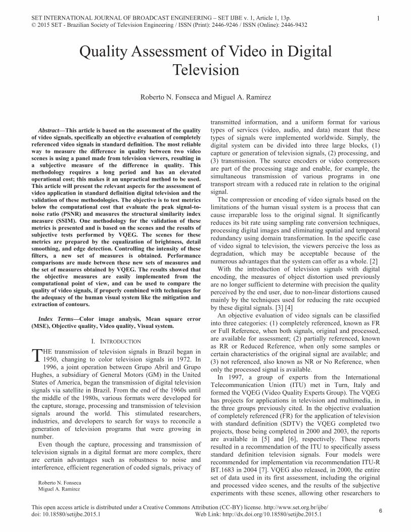
Fig. 2 shows an example of the system to obtain a video composite signal NTSC from their RGB nonlinear colors.

In this system, the reference signals G, B, and R must be synchronized with equal amplitude for the representation of an image without color information. These signals are usually described as corrections with gamma factor, represented in old documents like E’G, E’B, and E’R [19]. The definition of gamma correction is described by SMPTE, in SMPTE 170M-2004 [19] and by the International Telecommunication Union, in ITU-R BT709-5 in 2002 [20]. The equations that define this transfer function for the intervals 0.018<L<1 and 0.0812<V<1are:

4 89 Frr{ { (1)

. L B 8 E4 4 = =

5 4 = =C-

, 01 (2)

where V represents the electrical signal of components G, B, and R corrected by the gamma factor and L indicates the brightness when entering the capture system for each of the components Red (R), Green (G), and Blue (B). Outside the indicated interval the relationship is V=4.5L, then L=V/4.5.

According to Poyton, 1996 [16], the combination of two effects, those being the physical origin and the perceptive origin, were responsible for the gamma factor conception. The effect of the physical origin is related to the fact that the cathode ray tubes (CRT) used in television have an exponential transfer curve between the input voltage and output brightness, the perceptive origin factor is that human beings do not perceive linear variations of brightness.

These signals must be transformed into two components, luminance (Y) and chrominance (R-Y and B-Y). The term chrominance is defined as the difference between two colors with the same luminosity, one being a reference color [17]. After filtering to elimate high frequencies, the signals of different color (B-Y and R-Y) are sent to a quadrature modulator, which will modulate the I and Q vectors resulting in a phase modulation of the color subcarrier. This color subcarrier having been modulated is added to the luminance signal, as well as the synchronization signal of luminance, chrominance, deletion, and pedestal.

Fig. 2. Obtaining a composite video signal Fig. 3. Waveform of the composite video signal



4

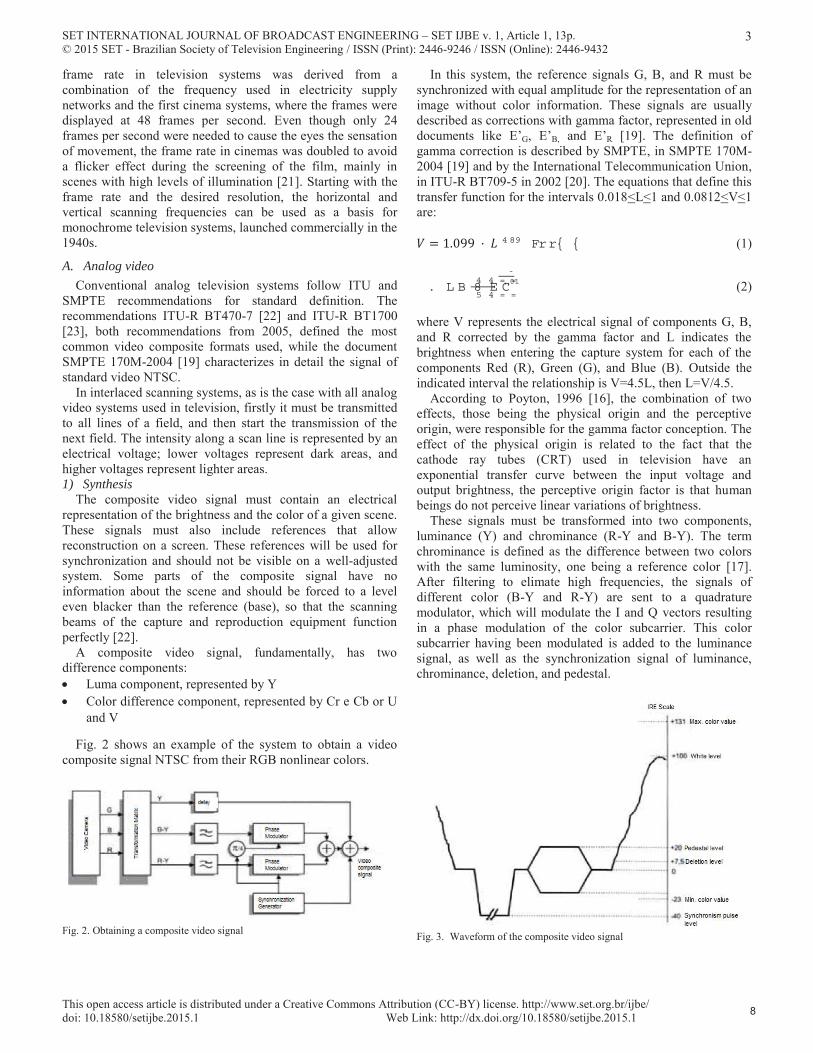
A representation of the electrical video signal can be seen in Figs. 3 and 4. In Fig. 3 the vertical axis represents the voltage, converted to the standard IRE, and the horizontal axis represent time, shown at an interval of the horizontal line. In Fig. 4 the representation is polar, where the magnitude is the color intensity and phase represents hue.

In terms of the spectral components, the video signal can be described by the sum of a luma signal as two color difference signals [19]. The following equation shows a composite video signal E’

M(t) formed by its components E’Y(t) U’(t) and V’(t).

(3)

The synchronization of these signals is of fundamental importance for the reproduction of video signals. The synchronization of analog television signal is done through horizontal and vertical synchronism pulses and saves color synchronism. These synchronism pulses are linked to each other by the definition of each pattern and color system. In NTSC-M systems, for example, the frequencies of color synchronization fsc, horizontal synchronization fH, and vertical synchronization fV are given by the following equations [19]:

(4)

(5)

(6)

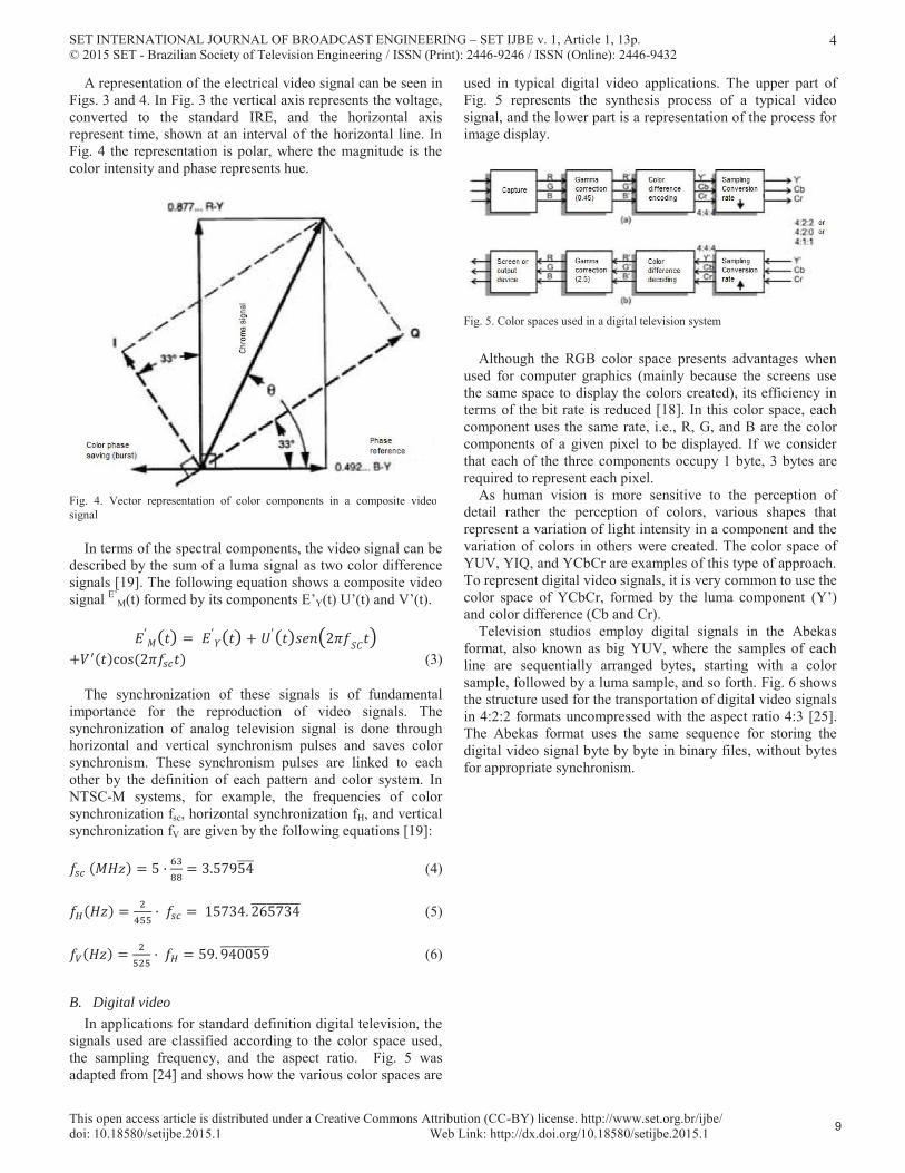
B. Digital video In applications for standard definition digital television, the

signals used are classified according to the color space used, the sampling frequency, and the aspect ratio. Fig. 5 wasadapted from [24] and shows how the various color spaces are

used in typical digital video applications. The upper part of Fig. 5 represents the synthesis process of a typical video signal, and the lower part is a representation of the process for image display.

Although the RGB color space presents advantages when used for computer graphics (mainly because the screens use the same space to display the colors created), its efficiency in terms of the bit rate is reduced [18]. In this color space, each component uses the same rate, i.e., R, G, and B are the color components of a given pixel to be displayed. If we consider that each of the three components occupy 1 byte, 3 bytes are required to represent each pixel.

As human vision is more sensitive to the perception of detail rather the perception of colors, various shapes that represent a variation of light intensity in a component and the variation of colors in others were created. The color space of YUV, YIQ, and YCbCr are examples of this type of approach. To represent digital video signals, it is very common to use the color space of YCbCr, formed by the luma component (Y’)and color difference (Cb and Cr).

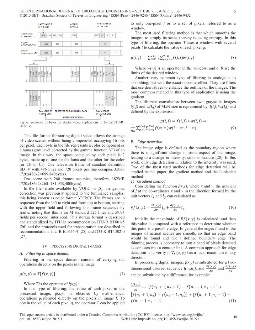
Television studios employ digital signals in the Abekas format, also known as big YUV, where the samples of each line are sequentially arranged bytes, starting with a color sample, followed by a luma sample, and so forth. Fig. 6 shows the structure used for the transportation of digital video signals in 4:2:2 formats uncompressed with the aspect ratio 4:3 [25].The Abekas format uses the same sequence for storing the digital video signal byte by byte in binary files, without bytes for appropriate synchronism.

Fig. 4. Vector representation of color components in a composite video signal

Fig. 5. Color spaces used in a digital television system



5

This file format for storing digital video allows the storage of video scenes without being compressed occupying 16 bits per pixel. Each byte in the file represents a color component or a luma (gray level corrected by the gamma function Y’) of an image. In this way, the space occupied by each pixel is 2 bytes, made up of one for the luma and the other for the color (or Cb or Cr). One television frame of standard definition SDTV with 486 lines and 720 pixels per line occupies 350kb (720x486x2=699,840bytes).

One scene with 260 frames occupies, therefore, 182MB (720x486x2x260=181,958,400bytes).

In the files made available by VQEG in [5], the gamma correction was previously applied to the luminance samples, this being known as color format Y’CbCr. The frames are in sequence from the left to right and from top to bottom, starting with the upper field and following this frame sequence by frame, noting that this is an M standard 525 lines and 59.94 fields per second, interlaced. This storage format is described and standardized by ITU in recommendation ITU-R BT601-5[26] and the protocols used for transportation are described in recommendations ITU-R BT656-4 [25] and ITU-R BT1302-0[27].

IV. PROCESSING DIGITAL IMAGES

A. Filtering in space domain Filtering in the space domain consists of carrying out

operations directly on the pixels in the image.

(7)

Where T is the operator of f(x,y). In this type of filtering, the value of each pixel in the

processed image, g(x,y), is obtained by mathematical operations performed directly on the pixels in image f. To obtain the value of each pixel g, the operator T can be applied

to only one-pixel f or to a set of pixels, referred to as a window.

The most used filtering method is that which smooths the images, to simply its scale, thereby reducing entropy. In this type of filtering, the operator T uses a window with several pixels f to calculate the value of each pixel g.

(8)

Where w(i,j) is an operator in the window, and a, b are the limits of the desired window.

Another very common type of filtering is analogous to smoothing, but with the exact opposite effect. They are filters that use derivatives to enhance the outlines of the images. The most common method in this type of application is using the gradient.

The discrete convolution between two grayscale images f(I,j) and w(I,j) of MxN size is represented by f(I,j)*w(I,j) and defined by the expression:

(9)

B. Edge detection The image edge is defined as the boundary region where

there is a significant change in some aspect of the image,leading to a change in intensity, color or texture [28]. In this work, only edge detection in relation to the intensity was used.Two of the most used methods for edge detection will be applied in this paper, the gradient method and the Laplacian method. 1) Gradient method

Considering the function f(x,y), where x and y, the gradient of f at the co-ordinates x and y in the direction formed by the unit vectors and can calculated as:

(10)

Initially the magnitude of is calculated, and then this value is compared with a reference to determine whether this point is a possible edge. In general the edges found in the images of natural scenes are smooth, so that an edge band would be found and not a defined boundary edge. The thinning process is necessary to turn a band of pixels detected as contours into a contour line. A common approach for edge detection is to verify if has a local maximum in any direction.

In processing digital images, f(x,y) is substituted for a two-dimensional discreet sequence f(n1,n2), and and can be substituted by a difference, for example:

. (11)

Fig. 6. Sequence of bytes for digital video applications in format ITU-RBT601-5



6

This difference can be seen as a discrete convolution between f(n1,n2) and the filter impulse response h(n1,n2). For the equation above, for example, the filter impulse response is given by the coefficients

-1 0 1

-1 0 1

-1 0 1

Specifically, in this case, this set of coefficients for specifying the Prewitt edge detection operator in the horizontal direction of an image (Prewitt, 1970 cited by Gonzalez and Woods, 2000) [1]. The contours in the vertical direction of a given image can be detected by another operator obtained by transposing h(n1,n2)=h(n2,n1). The fact that the contour detection can be given in a specific direction causes the operator to be called a directional operator. Non-directional operators can be developed by the discreet approximation of f(x,y). The following approximation was used by Duda and Hary, 1973 cited by Lim, 1990 [28] to define two different pairs of operators, called the Sobel operator and the Roberts operator.

(12)

where: and

The following are samples of the Sobel operators (3x3) and the Roberts operators (2x2):

-1 0 1

-2 0 2

-1 0 1

1 2 1

0 0 0

-1 -2 1

1 0

0 -1

0 1

-1 0

2) Laplacian method

Another way to detect contours in an image is to look for second order zero crossing differences. One issue that arises with this approach is that noise would be detected as contours, due to the sensitivity of the second derivative. One way to minimize this issue is by applying smoothing filters before submitting the image to contour detection. The equation below shows how to calculate the Laplacian of function f(x,y) [28]:

ˇt B:TÆ U; Lˇk B:TÆ U;oLtB:TÆ Q;

TtE

tB:TÆ U;

Ut (12)

Similar to what was seen in the gradient method, (9) can be approximated for digital images, represented by f(n1,n2), as follows:

ˇt B:TÆ U; \ ˇt B:JsÆJt ; LBTT:JsÆJt ; EB

UU:JsÆJt ; (13)

where BTT:JsÆJt ; and B

UU:JsÆJt ; can be approximated by

the difference in relation to previous and subsequent pixels, thus:

ˇ6 B:J5ÆJ6 ; LB:J5 E sÆ J6 ; EB:J5 F sÆ J6 ; EB:J5ÆJ6 Es; EB:J5ÆJ6 Fs; F vB : J5ÆJ6 ;. (14)

Similar to the gradient method, operators may be used to approximate the second-order derivative to be used in a discrete convolution. In the previous approach, for example, the Laplacian is calculated from a discrete convolution with the operator:

0 -1 0

-1 4 -1

0 -1 0

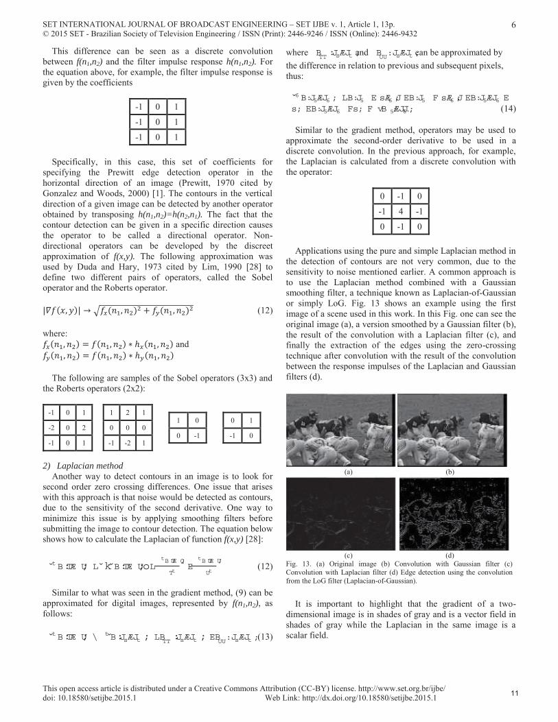
Applications using the pure and simple Laplacian method in the detection of contours are not very common, due to the sensitivity to noise mentioned earlier. A common approach is to use the Laplacian method combined with a Gaussian smoothing filter, a technique known as Laplacian-of-Gaussian or simply LoG. Fig. 13 shows an example using the first image of a scene used in this work. In this Fig. one can see the original image (a), a version smoothed by a Gaussian filter (b), the result of the convolution with a Laplacian filter (c), and finally the extraction of the edges using the zero-crossing technique after convolution with the result of the convolution between the response impulses of the Laplacian and Gaussian filters (d).

It is important to highlight that the gradient of a two-dimensional image is in shades of gray and is a vector field in shades of gray while the Laplacian in the same image is a scalar field.

(a) (b)

(c) (d)Fig. 13. (a) Original image (b) Convolution with Gaussian filter (c) Convolution with Laplacian filter (d) Edge detection using the convolution from the LoG filter (Laplacian-of-Gaussian).



7

V. VIDEO SIGNAL QUALITY

Usually, the viewer is interested in watching a two-dimensional representation of the real world that is as faithful as possible. The video signals are subject to degradation during capture, processing, storage, and transport. In composite video signals, analog television linear distortion and time invariants are inserted during these steps, allowing the utilization of a set of well-defined tests widely accepted by the community. Measured in terms of amplitude, frequency, and complete phase characterization of this type of signal and its distortions [29].

Recommendation ITU-R BT1204, 1995 [30] defines the techniques, test signals, and methodologies used to characterize these analog signals. Measures such as signal-to-noise ratio (S/N), differential gain (DG), phase gain (DP), impulsive characteristics (K2T and P/B), and linearity of the luma component are specified in this recommendation and are used to characterize video signals in the analog domain with high precision.

With the introduction of new digital techniques for the processing and compression of video signals, these measures are no longer sufficient to characterize the new forms of distortion inserted. According to Wang et al., 2003 [31]: "A video signal or image whose quality is being evaluated can be thought of as the sum of a perfect reference signal and an error signal". With this in mind, the most intuitive way to measure the video signal quality would be to quantify the error that is inserted in this signal. This task would be even simpler in the case of completely referenced video assessment since the reference signal is available.

According Jayant and Noll, 1984 [32]: "The evaluation of faithfulness or the degree of degradation that a given system causes in a video signal can be made objectively orsubjectively." The subjective evaluation involves a number of people in a controlled environment, following a certain methodology and being conducted by experts with extensive experience in this type of activity. Objective evaluation is performed automatically and requires an algorithm performing measurements of certain video signal characteristics, resulting in a measure of quality.

A. Subjective Evaluation In this type of evaluation, the scenes to be evaluated are

presented to a panel of observers, who judge the quality of the scenes presented in certain well-defined aspects, under certain conditions also previously set according to the application. Recommendation ITU-R BT.500-11 defines five basic methodologies for subjective quality assessment for standarddefinition television - SDTV: • Method 1:• DSIS (Double Stimulus Impairment Scale-) mainly used to measure the robustness of systems, or to characterize transmission failures; • Method 2:• DSCQS (Double-Stimulus Continuous Quality Scale) mainly used for measurement of degradation caused by systems with respect to a reference; • Alternative methodologies:• SS (Single Stimulus);

• SSCQE (Single Stimulus Continuous Quality Evaluation) used when you want to subjectively evaluate a scene without considering a reference; • SDSCE (Double-Simultaneous Stimulus for Continuous Evaluation) used for assessments where long scenes are required.

For applications in high-definition television (HDTV), video conferencing and multimedia applications, other ITU groups describe their evaluation methodologies. Pinson and Wolf carried out a comparison between these methodologies in 2003, verifying the sensitivity of each of them for certain applications, concluding that, among other things, for assessments using double stimuli (such as the DSCQS methodology) a duration of 15 seconds is a limiting factor due to the effect of the evaluators memory [33].

The evaluation of fully referenced digital television signal quality is of particular interest to the DSCQS methodology, in which pairs of scenes with short duration of time, typically 10 seconds, is presented to a panel of viewers, they attach notes to each scene pair . Using well-defined techniques for preparing the environment, choice of individuals, execution of experiments, and compilation of the results, the assessment methodology presents results in a consistent and well-defined way.

Although the evaluation of video signal quality in accordance with the perception of the viewer is defined by recommendation ITU-R-BT.500-11, new forms of assessment considering the compressed digital signal have been developed based on three main analysis techniques for the image quality in digital video [4]: • Use dynamic synthetic video signals for measuring the distortions caused by signal compression; • Make distortion measurements to determine how the original signal was distorted; • Use real video scenes and analyze a set of parameters to correlate with the subjective image quality [34] [35].

B. Objective Evaluation In this evaluation, there is a set of original and processed

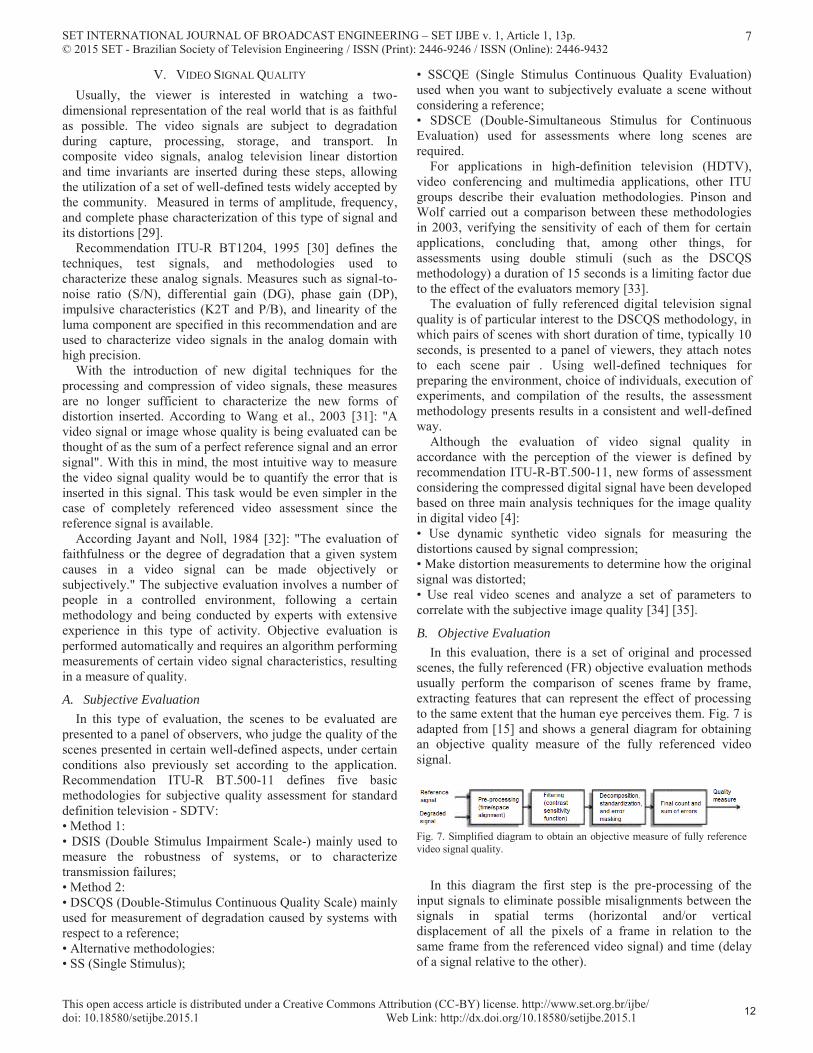
scenes, the fully referenced (FR) objective evaluation methods usually perform the comparison of scenes frame by frame, extracting features that can represent the effect of processing to the same extent that the human eye perceives them. Fig. 7 is adapted from [15] and shows a general diagram for obtaining an objective quality measure of the fully referenced video signal.

In this diagram the first step is the pre-processing of the input signals to eliminate possible misalignments between the signals in spatial terms (horizontal and/or vertical displacement of all the pixels of a frame in relation to the same frame from the referenced video signal) and time (delay of a signal relative to the other).

Fig. 7. Simplified diagram to obtain an objective measure of fully reference video signal quality.



8

1) ITU Models The objective of VQEG was to define and standardize the

correlations between the subjective evaluation of video quality and proposals for the objective evaluation of video quality from various laboratories. For the fully referenced (FR) objective evaluation in standard definition television - SDTV, VQEG performed two separate evaluations, called Phase I and Phase II. In the first phase VQEG analyzed 10 different algorithm proposals to objectively evaluate video quality, and in the second phase six proposals were evaluated. In 2000, VQEG released the final report on the first phase of the objective validation models for assessing video quality, concluding that none of the proposed models were materially superior to the traditional PSNR measure in all aspects, demanding a new phase of tests [5].

In 2003, the final report of the second phase was released, in which VQEG improved the tests performed and selected 6 models, suggesting the possibility of inclusion in ITU regulations, as the measures using PSNR were exceeded statistically [6]. In 2004, ITU published the recommendation ITU-R BT.1683, in which four models were described and approved for implementation [7]: • BTFR (British Telecommunication Full Reference)• EPSRN (Edge Peak Signal-to-Noise Ratio) • CPqDIES (Centro de Pesquisa e Desenvolvimento: Image Evaluation based on Segmentation) • NTIAVQM (National Telecommunications and Information Administration: Video Quality Metric)

The following will present the three distortion measures for objective evaluation using full reference that were utilized in this study, PSNR, SSIM, and S-CIELAB.

VI. DISTORTION MEASUREMENTS

A. PSNR The peak signal-to-noise ratio between two images or

PSNR can be defined as starting from the mean square root error calculated pixel by pixel. [1] The following equation shows the calculation of the mean square distortion between two images f e g in size M x N pixels in grayscale:

(14)

The PSNR has been used as a quality measurement reference for images and videos for many years. The following equation shows the calculation of PSNR between two images sampled with 8-bit resolution.

(15)

The main problem with this measure is that it does not take into account the limitations of the human visual system (HVS). The image compression algorithms and video compression algorithms use these limitations to act efficiently in the compression of these images and videos.

B. SSIM Based on structural similarity, this method was first

proposed by [37], but has been reviewed by [38] for better definition of the indexes. This approach has been published in literature in 2005 [39], and has been the basis for more improved methodologies for measuring the quality of an objective image like the E-SSIM [40] and the M-SSIM [41].

This measure is based on the assumption that the human visual system (HVS) is highly prepared to extract information about the structures present in its field of vision.

To define the SSIM index (Structural SIMilarity) between two images in grayscale f(i,j) and g(i,j), it is first necessary to define three basic quantities for each image block of 8x8 pixels of these images (1) comparing the luminance I(f,g), (2) comparing the contrast c(f,g), and (3) structure comparison s(f,g). The SSIM index for a pair of images is calculated by the following expression:

. (16)

For the calculation of the SSIM index, the author suggests a simplified version of (3), where . Equation (4) shows a simplified version of this expression, which was used in the experiments reported in this article.

(17)

Where: and are the average of the gray levels in each of the pair of images being compared, and and are the variances of these values, and refers to the cross-covariance gray levels of these images.

In a sequence containing T images or frames, the SSIM index is calculated by averaging S(f,g) as shown in the following equation:

. (18)

C. S-CIELAB The comparison of the quality of color images can be made

based on the differences between the opposite color space components L*, a*, and b*. The International Commission on Illumination, known as CIE (Commission Internationale de l'éclairage), in 1976, originally defined one approach for this type of evaluation. This standard has been updated by S014-4/E:2006, published in 2006 by CIE [42]. In this document, acolor space called CIE 1976 L* 2* b* is defined, which became known internationally as CIELAB. In this space, the component L* represents white to black variations and assumes values between 0 and 100. The component a* represents red tint changes to green, assuming values between -500 and +500 and the component b*, variations of yellow hue to blue, varying its value from - 200 to +200. The following equations specify the transformation between the color model based on three stimuli (CIEXYZ) and the CIELAB [24]:



9

(19)

Where X, Y, and Z are the three stimuli and Xn, Yn and Znare the values of the three stimuli of standard white (maximum value of X, Y, and Z).

CIELAB is, therefore, a color space formed by the components L*, a* and b*. The color difference between two CIELAB space images is calculated as a Euclidian distance, pixel to pixel and is referred to as ΔE.

The meaning of ΔE can be understood as follows: considering two colors closely defined by their coordinates L*, a* and b*, the ΔE value will be smaller the closer these colors are. The value of ΔE<1 indicates that the difference between these colors is not noticeable. The value of ΔE=1 indicates that the difference between these colors is less than can be perceived, being called JND (Just Noticeable Difference).

Several psychophysical experiments involving people's perception of differences between colors are conducted to arrive at a definition of ΔE. In 1996, Zhang and Wandell defined an extension of the CIELAB color space, called S-CIELAB. The difference of the S-CIELAB color space resulted in the measure ΔES [43].

To specify the color differences in the S-CIELAB space, smoothing filters are applied to the opposite color system components. In this work, for example, the filters that were adopted are described in [43]. The equation below shows the transformed CIEXYZ color system to the opposite color system formed by components O1, O2 and O3, which represent, respectively, the differences between white-black (W-B), red-green (R-G) and blue-yellow (B-Y).

(20) (20)

For each of these components, a two-dimensional filter is applied to adequately represent the sensitivity of human vision. The following equation describes the filter used in this work. The parameters k and ki were adopted as described in [43].

(21)

(21) Once filtered, the components O1, O2 and O3 of both

images, original and processed, are compared, resulting in the color difference S-CIELAB. The following equation shows how to calculate this difference:

. (22)

For a pair of video scenes composed of N images, each containing i lines and j columns, this process must be repeated N.i.j times. In this work, pairs of scenes, an original and a processed were subjected to the S-CIELAB comparison and a difference for each pair of scenes was obtained.

Tests for the application of this perceptual color difference measure in the assessment of images and video footage were made by Fonseca and Ramírez, 2008, and are available in [44]. In these tests, it was concluded that the use of S-CIELAB space for the assessment of color images significantly increases the degree of correlation with perception, but this does not happen for color video scenes.

VII. SIMULATION RESULTS

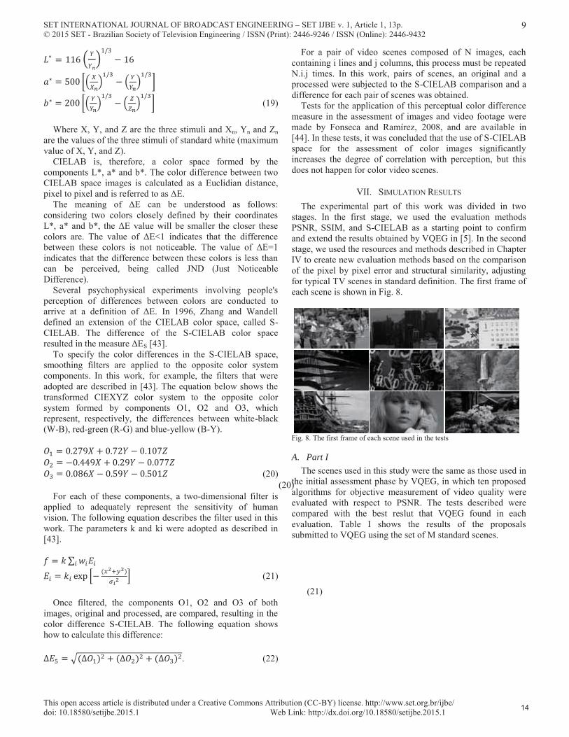
The experimental part of this work was divided in two stages. In the first stage, we used the evaluation methods PSNR, SSIM, and S-CIELAB as a starting point to confirm and extend the results obtained by VQEG in [5]. In the second stage, we used the resources and methods described in Chapter IV to create new evaluation methods based on the comparison of the pixel by pixel error and structural similarity, adjusting for typical TV scenes in standard definition. The first frame of each scene is shown in Fig. 8.

A. Part I The scenes used in this study were the same as those used in

the initial assessment phase by VQEG, in which ten proposed algorithms for objective measurement of video quality were evaluated with respect to PSNR. The tests described were compared with the best reslut that VQEG found in each evaluation. Table I shows the results of the proposals submitted to VQEG using the set of M standard scenes.

Fig. 8. The first frame of each scene used in the tests



10

It can be seen, as concluded by VQEG in [5], that none of the metrics were significantly better than PSNR, which is computationally more efficient than any other metric. Table II shows the comparison between the performance measurements obtained using PSNR, SSIM, and S-CIELAB in relation to the performance obtained by the P5 metric that is the best case that VQEG reported, utilizing the set of scenes used in this work. The P5 metric was developed by Winkler, 1999, and is described in [45]. In the Winkler metric, 4 different stages were used, including: (1) the perception of colors in opposite components, (2) spatial and temporal mechanism for filtering (3) masking and sensitivity of contrast and forms, and (4) response sensitivity of neurons in the primary visual cortex.

Although the results obtained by the P5 metric were better than those obtained using PSNR, SSIM, and S-CIELAB, it should be noted that only S-CIELAB uses the Cr and Cb components in the assessment. The assessment using SSIM and PSNR only includes the luma component (Y’), and they had similar results to those obtained with the use of color components. This is because the distortions inserted into the evaluated scenes cause similar degradation effects, to the perceptual point of view, in the three components Y’, Cb, and Cr.

Following are the individual effects of each scene (SRC) and each frame individually compared to the performance of each of the metrics so that the influence of these variables is clearly understandable.

This analysis was completed to have an understanding of how each scene individually contributes to the total mean error, as well as the contribution of each frame in the scene. In

the first experiment, the average error was obtained with the PSNR and SSIM metrics only using the luma component of the images. Table III shows the results obtained.

As can be seen, SRC19 is the biggest contributor to the total mean error. This scene contains images of an American football game, with horizontal camera movements and players. The errors in this type of scene type are not detectable by the human visual system with the same intensity that the PSNR and SSIM metrics detect.

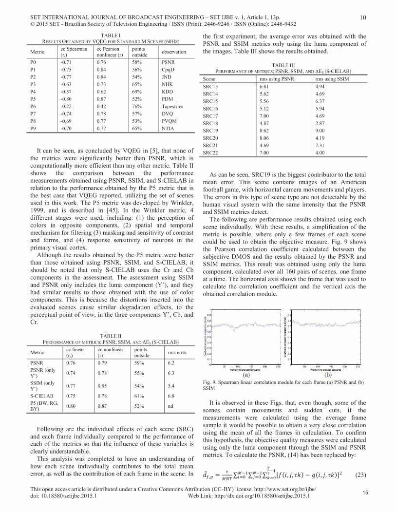
The following are performance results obtained using each scene individually. With these results, a simplification of the metric is possible, where only a few frames of each scene could be used to obtain the objective measure. Fig. 9 shows the Pearson correlation coefficient calculated between the subjective DMOS and the results obtained by the PSNR and SSIM metrics. This result was obtained using only the luma component, calculated over all 160 pairs of scenes, one frame at a time. The horizontal axis shows the frame that was used to calculate the correlation coefficient and the vertical axis the obtained correlation module.

It is observed in these Figs. that, even though, some of the scenes contain movements and sudden cuts, if the measurements were calculated using the average frame sample it would be possible to obtain a very close correlation using the mean of all the frames in calculation. To confirm this hypothesis, the objective quality measures were calculated using only the luma component through the SSIM and PSNR metrics. To calculate the PSNR, (14) has been replaced by:

(23)

TABLE IRESULTS OBTAINED BY VQEG FOR STANDARD M SCENES (60HZ)

Metric cc Spearman (rs)

cc Pearson nonlinear (r)

points outside observation

P0 -0.71 0.76 58% PSNRP1 -0.75 0.84 56% CpqDP2 -0.77 0.84 54% JNDP3 -0.63 0.73 65% NHKP4 -0.57 0.62 69% KDDP5 -0.80 0.87 52% PDMP6 -0.22 0.42 76% TapestriesP7 -0.74 0.78 57% DVQP8 -0.69 0.77 53% PVQMP9 -0.70 0.77 65% NTIA

TABLE IIPERFORMANCE OF METRICS; PSNR, SSIM, AND ΔES (S-CIELAB)

Metric cc linear (rs)

cc nonlinear (r)

points outside rms error

PSNR 0.76 0.79 59% 6.2PSNR (only Y’) 0.74 0.78 55% 6.3

SSIM (only Y’) 0.77 0.85 54% 5.4

S-CIELAB 0.75 0.78 61% 6.8P5 (BW, RG, BY) 0.80 0.87 52% nd

TABLE IIIPERFORMANCE OF METRICS; PSNR, SSIM, AND ΔES (S-CIELAB)

Scene rms using PSNR rms using SSIMSRC13 6.81 4.94SRC14 5.62 4.69SRC15 5.56 6.37SRC16 5.12 5.94SRC17 7.00 4.69SRC18 4.87 2.87SRC19 8.62 9.00SRC20 8.06 4.19SRC21 4.69 7.31SRC22 7.00 4.00

Fig. 9. Spearman linear correlation module for each frame (a) PSNR and (b) SSIM



11

where f(i,j,τk) is the pixel value at coordinate (i,j) of frame τkof the scene f; g(i,j,τk) is the pixel value at coordinate (i,j) of frame τk of scene g; τ is the sub-sampling value, or is only measured in τ frames.

The calculation of the SSIM mean value between scenes has similarly been completed, by substituting (18) for:

˝ˆ @ 4

¯?55 : BÆ C ;. (24) (24)

Table IV shows the results obtained by the objective metrics PSNR and SSIM using only Y’ values for τ equal to 2, 5, 10, 20, 50 and 100, ie 50%, 20%, 10%, 5% , 2% and 1% of total 260 frames in each of the scenes.

These results suggest that for applications in SDTV two simplifications can be made without significant loss of performance in the tested metrics: • Use only the luma component (Y’) and • Use only 5% of the frames in the scene.

B. Part II In this part of the work, the experiments were performed to

verify how a metric can have its correlation with the subjective measure improved with a pre-set adjustment to the scenes to be evaluated. There are three different types of adjustments in this work: (1) standardization of brightness, (2) filter enhancement for edge detection, and (3) a smoothing filter.

Table V shows the results obtained after standardization of each frame in all scenes. The first line refers to the PSNR performance results applied only in luma without the standardization of brightness and the second line refers to the PSNR performance only in luma with the brightness differences corrected.

Edge detection was completed using the filtering techniques presented in [36]. Five different methods for extracting contours were tested: (1) Sobel, (2) Canny, (3) Roberts, (4) Prewitt, and (5) Laplacian of Gaussian (also known as LoG). The performance metric was performed on images containing only the original image contours, which are shown in Table VI.

Note the significant improvement in correlation with the subjective measure when using Sobel and Roberts edge detection methods. This is consistent with the fact that the human visual system is adapted to extract the structural forms of the images that are captured by the eyes. These methods for extracting contours when optimally applied require few computational resources.

The effects of using a smoothing filter before the execution of the PSNR and SSIM metrics in correlation with the subjective measurements are shown in Tables VII and VIII.

TABLE IVPERFORMANCE OF EACH METRIC ACCORDING TO THE NUMBER OF FRAMES

USED

Metric Frames used

ccSpearman (rs)

cc Pearson nonlinear

points outside

rms errors

Y’_PSNR 100% -0.74 0.78 56% 6.4Y’_PSNR 50% -0.74 0.78 57% 6.4Y’_PSNR 20% -0.74 0.79 57% 6.3Y’_PSNR 10% -0.74 0.78 58% 6.3Y’_PSNR 5% -0.74 0.78 59% 6.3Y’_PSNR 2% -0.72 0.77 61% 6.6Y’_PSNR 1% -0.69 0.74 61% 6.9Y’_SSIM 100% -0.77 0.85 53% 5.4Y’_SSIM 50% -0.77 0.85 55% 5.5Y’_SSIM 20% -0.77 0.85 51% 5.4Y’_SSIM 10% -0.76 0.85 52% 5.5Y’_SSIM 5% -0.76 0.85 52% 5.5Y’_SSIM 2% -0.76 0.84 54% 5.6Y’_SSIM 1% -0.75 0.83 56% 5.8

TABLE VPERFORMANCE COMPARISON OF PSNT AFTER STANDARDIZATION

Metric cc Spearman (rs)



Y-PSNR -0.74 0.78 55% 6.3

Y-PSNR standardized -0.71 0.75 61% 6.8

TABLE VIPERFORMANCE OF EACH METRIC ACCORDING TO THE NUMBER OF FRAMES

USED

Detection Method

cc Spearman (rs)



Sobel -0.78 0.84 52% 5.5Canny -0.57 0.64 71% 8.2Roberts -0.80 0.84 52% 5.5Prewitt -0.79 0.84 53% 5.5LoG -0.70 0.77 66% 6.8

TABLE VIIEFFECT OF A SMOOTHING FILTER ON THE PERFORMANCE OF THE DMOSPSNR

MEASURE COMPARED TO THE DMOS MEASURE

Pof the filter cc Spearman cc nonlinear points

outside rms error

no filter -0.74 0.77 55% 6.30.5 -0.76 0.81 55% 6.01.0 -0.75 0.79 53% 6.21.5 -072 0.76 54% 6.5

TABLE VIIIEFFECT OF A SMOOTHING FILTER ON THE PERFORMANCE OF THE DMOSSSIM

MEASURE COMPARED TO THE DMOS MEASURE

Pof the filter cc Spearman cc nonlinear points

outside rms error

no filter -0.57 0.59 70% 8.40.5 -0.76 0.85 49% 5.31.0 -0.78 0.86 51% 5.11.5 -0.77 0.85 54% 5.4



12

VIII. CONCLUSION

A comparison of the objective evaluation metrics of video quality was presented. The performance metrics PSNR, SSIM, and S-CIELAB, were presented. It has been shown that for typical TV scenes in standard definition, subjected to typical distortions for this type of application, that it is still possible for more simplification of the types of metrics used to be completed, enabling their use in practical applications in real time. In addition, the results of the comparison with the subjective measurements showed that these simple metrics can be significantly improved when better adapted to the spatial contrast sensitivity and the structural recognition capability of the human visual system.

The adaptation to spatial contrasts was completed with the use of image smoothing filters. The image recognition structures were tested with the use of filters for extracting contours and also with a metric that has this intrinsic characteristic (SSIM).

These metrics are not able to replace the subjective evaluation of video quality, but complement this type of evaluation, estimating its results to a correlation of around 85%. Other approaches suggested to continue this work: • Provide other databases with previously evaluated video scenes to supply the scientific community with shared resources of good quality, like the VQEG scenes used in this work; • Test other filter types that are related to the extraction of structural information of video scenes; • Complete the same tests for applications in high-definition television HDTV; • Partially referenced or even non-referenced implementations can be tested, visualizing applications in remote monitoring.

REFERENCES

[1] R.C. Gonzalez and R. E. Woods, Processamento de Imagens Digitais, 1st ed,. São Paulo, Brazil: Edgard Blücher, 2000, p. 509.[2] J. Watkinson, “The Art of Digital Video,”. Revista de radioifusão vol. 03, no. 0330, p. 774, 2000.[3] M. Pinson and S. Wolf, “A new standardized method for objectively measuring video quality,” IEEE Transactions on Broadcasting, vol. 50, no. 3, pp. 312–322, 2004. [4] W. Y. Zou and P. J. Corriveau, “Methods for evaluation of digital television picture quality,” presented at the 138th SMPTE Technical Conference and World Media, 1996. [5] Video Quality Experts Group, “Final Report from the Video Quality Experts Group on the Validation of Objective Models of Video Quality Assessment,” VQEG, March 2000. Available: <ftp://vqeg.its.bldrdoc.gov/>. [6] Video Quality Experts Group, “Final Report on the Validation of Objective Models of Video Quality Assessment, Phase II,” March. 2003. Available: <ftp://vqeg.its.bldrdoc.gov/>. [7] Objective perceptual vqm techniques for digital broadcast television in the presence of a full reference, Recommendation ITU-R BT1683, 2004. [8] I. P. Gunawan and M. Ghanbari, “Reduced-reference video quality assessment using discriminative local harmonic strength with motion consideration,” IEEE Transactions on Circuits and Systems for Video Technology, vol. 18, no. 1, pp. 71–83, 2008. [9] E. P. ONG et al, “Video quality metrics - an analysis of low bit-rate videos,” in IEEE International Conference on Acoustics, Speech, and Signal Processing - ICASSP, vol. 1, pp. I–889–I–892, 2007. [10] H. Sheikh and A. Bovik, “Image information and visual quality,” IEEE Transactions on Image Processing, vol. 15, no. 2, pp. 430–444, 2006. [11] K. Seshadrinathan, and A. C. Bovik, “A structural similarity metric for video based on motion models,” in IEEE International Conference on Acoustics, Speech, and Signal Processing, vol. 1, no. 1, pp. 869–872, 2007.

[12] J. Guo, M. V. Dyke-Lewis, and H. R. Myler,” Gabor difference analysis of digital video quality,” IEEE Transactions on Broadcasting, vol. 50, no. 3, 2004. [13] Methodology for the assessment of the quality of television pictures,Recommendation ITU-R BT500-11, 2002. [14] Subjective video quality assessment methods for multimedia applications, Recommendation ITU-T P910, 2008. [15] T. N. Pappas and R. J. Safranek, “Perceptual criteria for image quality evaluation,” Handbook of image and video processing. Academic Press, 2000. ch. 8, sec. 2, pp. 669–684. [16] C. A. Poynton. (1996). A Technical Introduction To Digital Video.[Online]. Available: <http://www.poynton.com/ PDFs/GammaFAQ.pdf>. [17] K. B. Benson and J. K. Whitaker, Television Engineering Handbook:Featuring HDTV systems. New York: Mc Graw-Hill, 1992. [18] K. Jack, Video Demystified: A Handbook for the Digital Engineer. 3rd ed., Eagle Rock: LLH Technology Publishing, 2001, p. 759. [19] Composite analog video signal, SMPTE 170M-2004, 2004. [20] Parameter values for the HDTV standards for production and international programme exchange, Recommendation ITU-R BT709-05,2002. [21] B. Grob, Televisão e Sistemas de Vídeo, 5th ed,. Rio de Janeiro, Brazil: Guanabara S.A, 1989, p. 385. [22] Conventional analogue television systems, Recommendation ITU-RBT470-7, 2005. [23] Characteristics of composite video signals for conventional analogue television systems, Recommendation ITU-R BT1700, 2005. [24] C. A. Poynton. (1997). Frequently Asked Questions about Color.[Online]. Available: <http://www.poynton.com/PDFs/ColorFAQ.pdf>. [25] Interfaces for digital component video signals in 525-line and 625-line television systems operating at the 4:2:2 level of recommendation ITU-RBT.601 (part a), Recommendation ITU-R BT656-4, 1998. [26] Studio encoding parameters of digital television for standard 4:3 and wide-screen 16:9 aspect ratios, Recommendation ITU-R BT601-5, 1995. [27] Interfaces for digital component video signals in 525-line and 625-line television systems operating at the 4:2:2 level of recommendation ITU-RBT.601 (part b), Recommendation ITU-R BT1302-0, 1997. [28] J.S. Lim, Two-Dimensional Signal and Image Processing, 2nd ed., Englewood Cliffs: [s.n.], 1990, p. 694. [29] D. K. Fibush, “Tutorial paper - video testing in a dtv world,” SMPTE Journal Society of Motion Pictures and Television Engineers, no. 109, pp.661–667, 2000. [30] Measuring methods for digital video equipment with analogue input/output, Recommendation ITU-R BT1204, 1995. [31] Z. Wang, H. R. Sheikh, and A. C. Bovik, “Objective video quality assessment,” in The Handbook of Video Databases: Design and applications, 1st ed., Austin: [s.n.], 2003. [32] N. Jayant and P. Noll, Digital Coding of Waveforms: Principles and Applications to Speech and Video. 2nd ed., Englewood Cliffs: [s.n.], 1984, p. 688. [33] M. H. Pinson and S. Wolf, “Comparing subjective video quality testing methodologies,” in VCIP, [S.l.: s.n.], 2003, pp. 573–582. [34] M. C. Q. Farias, M. Carli, and S. K. K. Mitra, “Video quality objective metric using data hiding,” in IEEE International Workshop on Multimedia and Signal Processing, [S.l.: s.n.], 2002. [35] M. C. Q. Farias, J. M. Foley, and S. K. Mitra,” Perceptual contributions of blocky blurry and noisy artifacts to overall annoyance,” in International Conference on Multimedia and Expo, Baltimore: [s.n.], 2003. [36] R. Arthur, “Avaliação Objetiva de Codecs de Video,” M.S. thesis, UNICAMP, Campinas, São Paulo, Brazil, 2002. [37] Z. Wang and A. C. Bovik, “A universal image quality index,” IEEE Signal Processing Letters, vol. 9, pp. 81–84, March. 2002. [38] Z. Wang, L. Lu, and A. C. Bovik, “Video quality assessment using structural distortion measurement,” in International Conference on Image Processing, vol. 3, pp 65-68, [S.l.: s.n.], 2002. [39] Z. Wang, A. C. Bovik, and E. P. Simoncelli, “Structural approaches to image quality assessment,” in Handbook of Image and Video Processing, 2nded., San Diego: [s.n.], 2005. [40] G. H. Chen et al. “Edge-based structural similarity for image quality,” in IEEE Transactions on Acoustics, Speech, and Signal Processing, vol. 2, no. 1, pp. II–II, 2006. [41] Z. Wang, E. P. Simoncelli, and A. C. Bovik, “Multiscale structural similarity for image quality assessment,” in Conference Record of the Thirty-Seventh Asilomar Conference on Signals, Systems and Computers, vol. 2, pp. 1398-1402, [S.l.: s.n.], 2003.



13

[42] Colorimetry - Part 4: Cie 1976 l*a*b* colour spaces, CIE S 014-4/E:2007, 2007. [43] X. Zhang and B. A. Wandell, “A spatial extension of cielab for digital color image reproduction,” Society for Information Display Symposium Technical Digest, vol. 27, pp. 731–734, 1996. [44] Roberto N. Fonseca and Miguel A. Ramírez, “Using SCIELAB for image and video quality evaluation,” in ISCE 2008. IEEE International Symposium, 2008, pp.1 – 4. [45] S. Winkler, “A perceptual distortion metric for digital color video,” inProc. SPIE Human Vision and Electronic Imaging Conference, San Jose: [s.n.], 1999, vol. 3644, pp. 175–184.

Cite this article: Fonseca, Roberto N. and Ramirez, Miguel A. .; 2015.Quality Assessment of Video in Digital Television. SET INTERNATIONAL JOURNAL OF BROADCAST ENGINEERING. ISSN Print: 2446-9246 ISSN Online: 2446-9432. doi: 10.18580/setijbe.2015.1. Web Link: http://dx.doi.org/10.18580/setijbe.2015.1

Documents

Quality Assessment of Video in Digital Television - SET … · Index Terms—Color image analysis, Mean square error (MSE), ... for applications in television and multimedia, in