PAPER

Quantification of dissipation and deformation inambient atomic force microscopyTo cite this article: Sergio Santos et al 2012 New J. Phys. 14 073044

 

View the article online for updates and enhancements.

You may also likeFermi-polaron-like effects in a one-dimensional (1D) optical latticeM J Leskinen, O H T Nummi, F Massel etal.

-

Time independent universal computingwith spin chains: quantum plinko machineK F Thompson, C Gokler, S Lloyd et al.

-

Coupled activity-current fluctuations inopen quantum systems under strongsymmetriesD Manzano, M A Martínez-García and P IHurtado

-

Recent citationsAdvances in dynamic AFM: Fromnanoscale energy dissipation to materialproperties in the nanoscaleSergio Santos et al

-

Single cycle and transient forcemeasurements in dynamic atomic forcemicroscopyKarim Gadelrab et al

-

Size Dependent Transitions in NanoscaleDissipationSergio Santos et al

-

This content was downloaded from IP address 153.166.7.69 on 27/11/2021 at 06:03

T h e o p e n – a c c e s s j o u r n a l f o r p h y s i c s

New Journal of Physics

Quantification of dissipation and deformation inambient atomic force microscopy

Sergio Santos1,3, Karim R Gadelrab1,3, Victor Barcons2, MarcoStefancich1 and Matteo Chiesa1,4

1 Laboratory of Energy and Nanosciences, Masdar Institute of Science andTechnology, Abu Dhabi, United Arab Emirates2 Departament de Disseny i Programacio de Sistemes Electronics,UPC—Universitat Politecnica de Catalunya Av. Bases, 61, 08242 Manresa,SpainE-mail: mchiesa@masdar.ac.ae

New Journal of Physics 14 (2012) 073044 (12pp)Received 18 April 2012Published 20 July 2012Online at http://www.njp.org/doi:10.1088/1367-2630/14/7/073044

Abstract. A formalism to extract and quantify unknown quantities such assample deformation, the viscosity of the sample and surface energy hysteresisin amplitude modulation atomic force microscopy is presented. Recoveringthe unknowns only requires the cantilever to be accurately calibrated and thedissipative processes occurring during sample deformation to be well modeled.The theory is validated by comparison with numerical simulations and shownto be able to provide, in principle, values of sample deformation with picometerresolution.

S Online supplementary data available from stacks.iop.org/NJP/14/073044/mmedia

The capacity of atomic force microscopy (AFM) to investigate energy dissipation in thenanoscale has been well demonstrated [1–8]. In amplitude modulation (AM) AFM, the principlerelies in monitoring the perturbed phase ϕ and oscillation amplitude A of the cantilever relativeto the drive. In particular, the energy dissipated per cycle in the interaction Edis can be calculatedby applying the energy conservation principle. Accounting for the fundamental frequency ω

only, Cleveland et al [4] found that

〈Edis〉 =πk A0 A

Q

[sin (φ) −

A

A0

], (1)

3 These authors contributed equally to this work.4 Author to whom any correspondence should be addressed.

New Journal of Physics 14 (2012) 0730441367-2630/12/073044+12$33.00 © IOP Publishing Ltd and Deutsche Physikalische Gesellschaft

2

where A0 is the free amplitude, k is the spring constant and Q is the Q factor due to dissipationwith the medium. While, in ambient conditions, higher harmonics have been shown to reduceto a few angstroms or fractions of angstroms of amplitude, these can still be accounted for inorder to increase the accuracy of (1). According to Tamayo [9],

〈Edis〉 =πk A0 A

Q

[sin(ϕ) −

1

A0 A1

∑n≥1

n2 A2n

], (2)

where An are the amplitudes of the harmonics (A = A1 in (1)). Further accuracy in Edis could beobtained by considering the second mode of oscillation [10, 11]. Other advances in the in situcalibration of k, Q, the natural oscillation frequency ω0 and the tip radius R have been made inparallel and we consider these as known experimental quantities in the rest of this work [12–14].For simplicity, we further set ω = ω0 throughout. With all, Edis in (1) and (2) is a quantitythat accounts for the net energy dissipated but the expression cannot distinguish betweendissipative processes. Thus, effort has been put into interpreting and/or decoupling the differentcontributions to Edis over the last few years. For example, Garcia et al [1, 2, 15] found that it isdEdis/dA that provides information about the nature of the dissipative mechanisms. In particular,during sample deformation, two main dissipative processes have been identified, namely surfaceenergy γ hysteresis and viscoelasticity. It was also proposed that in the repulsive force regimeand by sufficiently increasing the value of the free amplitude A0, the dissipation and processesoccurring during sample deformation could be probed; both sample deformation and dissipationscale with the free amplitude [1, 16, 17]. Also note that prevailing long-range dissipativeprocesses, such as the hysteretic formation and rupture of the capillary neck that might occurin ambient conditions, should be relatively independent of operational parameters and can bereadily probed in the attractive force regime [3, 18]. More recently, viscoelastic heterogeneityin a metallic glass has been mapped with nanoscale resolution using the dEdis/dA approach.Such experiments provide fundamental experimental information that might be used to fill thegap between atomic models and macroscopic glass properties [8]. Moreover, due to the goodagreement between the dEdis/dA method and experiment [1, 2, 19], several other approaches toidentifying and decoupling dissipative processes [20, 21], some of these being quantitative [21],have recently been proposed. Nevertheless, quantitative approaches might have disadvantagessuch as the requirement to select an appropriate model for the conservative component of theforce or other dissipative channels, in particular in the long range where mechanical contactdoes not occur [21, 22]. Garcia et al further found that viscoelastic and surface energy hysteresisprocesses could be well modeled by considering (i) the variation in the adhesion force duringtip approach FAD(approach) = −4pRγa and tip retraction FAD(retraction) = −4pRγr, where therespective surface energies are γa and γr(γr > γa) and (ii) the Voigt model for the viscoelasticforce Fη [2, 19, 23],

Fη = −η(Rδ)1/2δ, (3)

where δ is the instantaneous tip–sample deformation, δ is the tip velocity during deformationand η is the viscosity of the materials in contact. Note that tip–sample deformation here refers tothe fact that when the tip and the sample are in mechanical contact, both materials deform [24].If the elastic modulus of the tip is much greater than that of the sample the deformation can beassociated with the sample alone. Nevertheless, in this work, the terms sample deformation and

New Journal of Physics 14 (2012) 073044 (http://www.njp.org/)

3

tip–sample deformation will be used interchangeably to refer to tip–sample deformation andwill be written as δ. The dissipative term of the adhesion force Fα can also be written as

Fα = −4π Rγα = FADα, (4)

where α = γr/γa − 1 accounts for differences in γa and γr and where γ = γa and FAD = −4pRγ .More recent studies also support the validity of these expressions for a variety of sampleswhere large values of α have been interpreted as the capacity to restructure the atomicbonds of the surfaces in contact [7, 21, 25]. It is clear that the interpretation of α and η

requires an understanding of dissipation in a dynamic nanoscale contact. However, here, weassume that the two main dissipative channels during sample deformation are surface energyγ hysteresis and viscoelasticity. In particular, we further assume that these two processesare well modeled with (3) and (4), respectively. This is done as a first approximation tothe problem with the understanding that future experimentation and testing should establishwhether these expressions are valid in general or whether slight modifications will be required.Then, we set to provide the fundamental relationships between the known dynamic (static)parameters, i.e. A, A0, ω and z0, where z0 is the mean cantilever deflection, Q, and ϕ (kand R) and what are termed, from now on, the sample’s dissipative properties, that is, α

and η. The formalism developed in this work further provides the means to quantify themaximum tip–sample deformation in one cycle δM, this typically being another fundamentalunknown in experiments. Our simulations show that, with the proposed formalism, δM canbe potentially quantified with great accuracy and down to picometer resolution with the useof known experimental parameters. In particular, the framework depends on the relationshipsbetween the magnitude of the energy dissipated in one cycle 〈Edis〉, that is, (1) or (2), andthe dependencies of the dissipative channels, i.e. viscoelasticity and surface energy hysteresis,on δM and on the oscillation amplitude A. Integration of (3) and (4) shows that the energydissipated in one cycle via surface energy hysteresis Eα depends linearly on δM ,whereas thedependence is quadratic for the energy dissipated via viscoelasticity Eη. A great advantage ofthe present approach is that it is independent of the nature of the tip–sample interaction providedthe two main dissipative processes during sample deformation are surface energy hysteresisand/or viscoelasticity. Experimentally, one could first use the dEdis/dA method [1, 8, 20] toestablish whether these dissipative processes are dominant and then quantify the dissipativeparameters and the tip–sample deformation with the present formalism. It should be noted,however, that only the energy dissipated during sample deformation should be decoupled fromthe energy dissipated during non-contact dissipative processes. That is, care should be takenwhen establishing whether the energy is being dissipated during sample deformation alone. Inthis respect, several methodologies are proposed at the end of this work. One of the proposedmethodologies is used satisfactorily in a numerical example. In summary, this work provides aframework to directly obtain quantitative information about fundamental dissipative propertiesof the sample with the use of known experimental parameters alone.

Let us begin by writing the relationships between δM and the energy dissipated in the twoprocesses (3) and (4). It follows that

Eα = −4π Rγα

∫ δ=0

δ=δM

dδ = −FADαδM, (5)

where, as stated, Eα is the energy dissipated due to surface adhesion hysteresis in one cycle. Inorder to express the energy dissipated per cycle via viscoelasticity Eη as a function of δM use is

New Journal of Physics 14 (2012) 073044 (http://www.njp.org/)

4

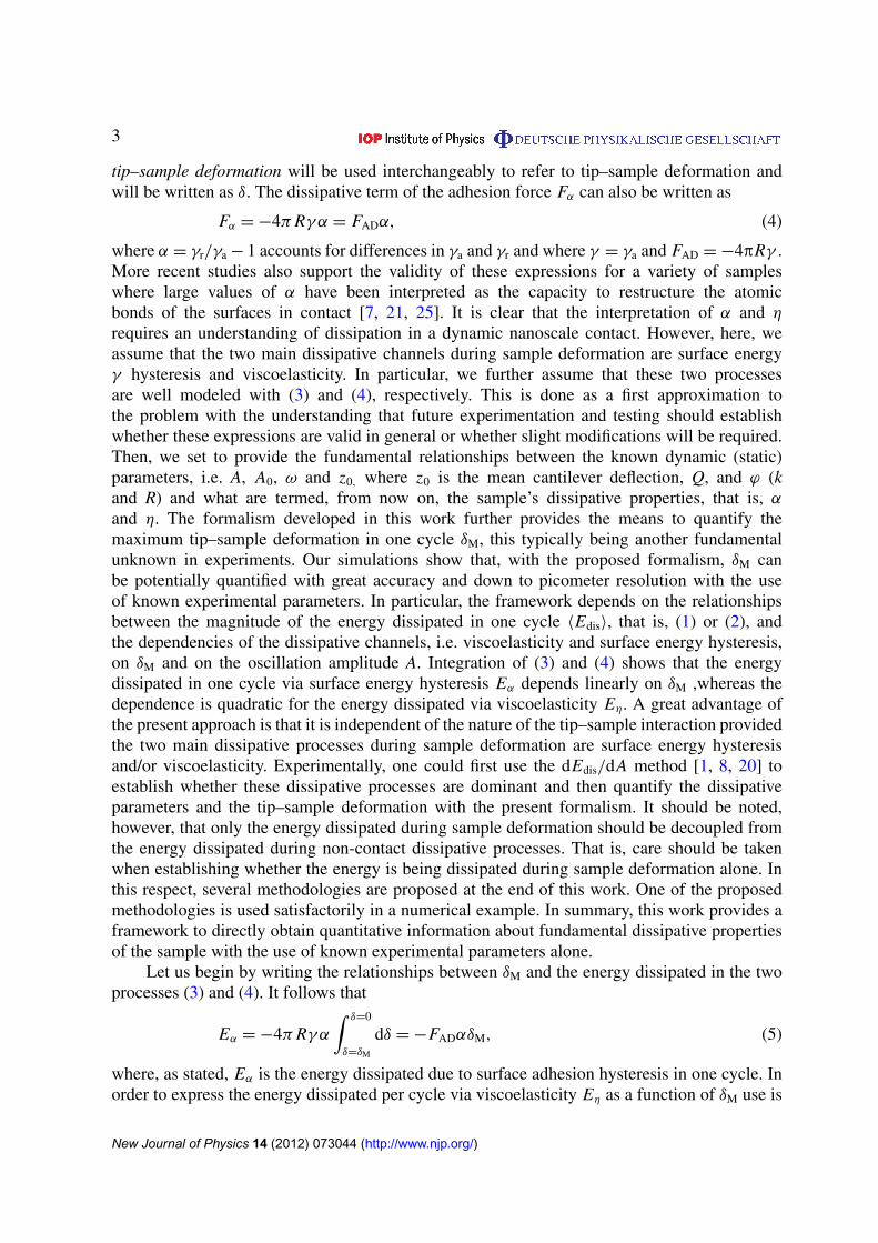
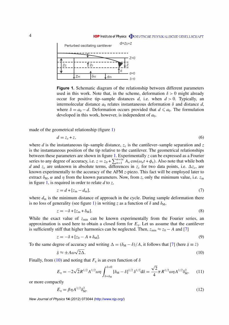
Figure 1. Schematic diagram of the relationship between different parametersused in this work. Note that, in the scheme, deformation δ > 0 might alreadyoccur for positive tip–sample distances d, i.e. when d > 0. Typically, anintermolecular distance a0 relates instantaneous deformation δ and distance d,where δ = a0 − d. Deformation occurs provided that d 6 a0. The formulationdeveloped in this work, however, is independent of a0.

made of the geometrical relationship (figure 1)

d = zc + z, (6)

where d is the instantaneous tip–sample distance, zc is the cantilever–sample separation and zis the instantaneous position of the tip relative to the cantilever. The geometrical relationshipsbetween these parameters are shown in figure 1. Experimentally z can be expressed as a Fourierseries to any degree of accuracy, i.e. z = z0 +

∑n=∞

n=1 An cos(ωnt + φn). Also note that while bothd and zc are unknown in absolute terms, differences in zc for two data points, i.e. 1zc, areknown experimentally to the accuracy of the AFM z-piezo. This fact will be employed later toextract δM, α and η from the known parameters. Now, from z, only the minimum value, i.e. zm

in figure 1, is required in order to relate d to z,

z = d + [zm − dm], (7)

where dm is the minimum distance of approach in the cycle. During sample deformation thereis no loss of generality (see figure 1) in writing z as a function of δ and δM,

z = −δ + [zm + δM]. (8)

While the exact value of zmin can be known experimentally from the Fourier series, anapproximation is used here to obtain a closed form for Eη. Let us assume that the cantileveris sufficiently stiff that higher harmonics can be neglected. Then, zmin ≈ z0 − A and [7]

z = −δ + [z0 − A + δM]. (9)

To the same degree of accuracy and writing 1 = (δM − δ)/A, it follows that [7] (here.

δ ≡.z)

.

δ ≈ ±Aω√

21. (10)

Finally, from (10) and noting that Fη is an even function of δ

Eη = −2√

2R1/2 A1/2ωη

∫ δ=0

δ=δM

[δM − δ]1/2 δ1/2dδ =

√2

4π R1/2ωηA1/2δ2

M, (11)

or more compactly

Eη = βηA1/2δ2M, (12)

New Journal of Physics 14 (2012) 073044 (http://www.njp.org/)

5

where β is a function of known parameters (β =√

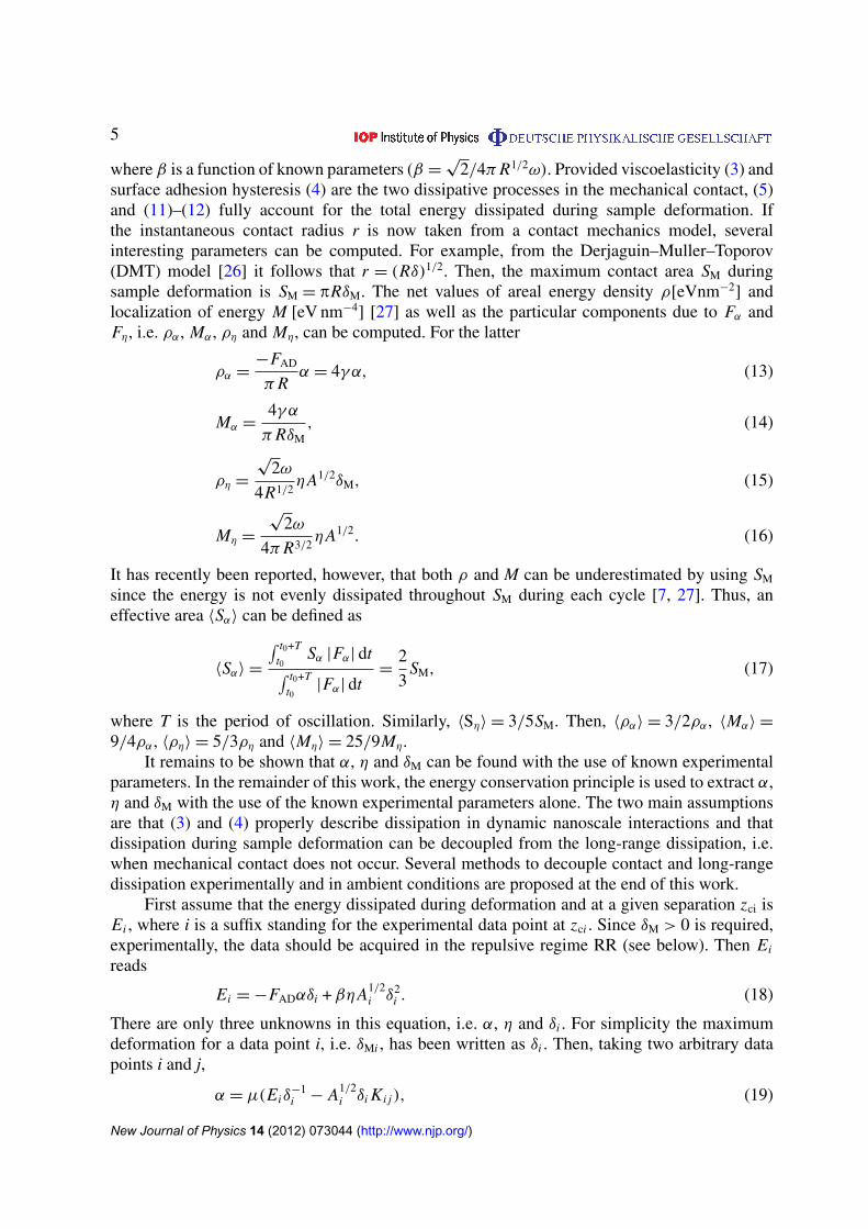
2/4π R1/2ω). Provided viscoelasticity (3) andsurface adhesion hysteresis (4) are the two dissipative processes in the mechanical contact, (5)and (11)–(12) fully account for the total energy dissipated during sample deformation. Ifthe instantaneous contact radius r is now taken from a contact mechanics model, severalinteresting parameters can be computed. For example, from the Derjaguin–Muller–Toporov(DMT) model [26] it follows that r = (Rδ)1/2. Then, the maximum contact area SM duringsample deformation is SM = pRδM. The net values of areal energy density ρ[eVnm−2] andlocalization of energy M [eV nm−4] [27] as well as the particular components due to Fα andFη, i.e. ρα, Mα, ρη and Mη, can be computed. For the latter

ρα =−FAD

π Rα = 4γα, (13)

Mα =4γα

π RδM, (14)

ρη =

√2ω

4R1/2ηA1/2δM, (15)

Mη =

√2ω

4π R3/2ηA1/2. (16)

It has recently been reported, however, that both ρ and M can be underestimated by using SM

since the energy is not evenly dissipated throughout SM during each cycle [7, 27]. Thus, aneffective area 〈Sα〉 can be defined as

〈Sα〉 =

∫ t0+Tt0

Sα |Fα| dt∫ t0+Tt0

|Fα| dt=

2

3SM, (17)

where T is the period of oscillation. Similarly, 〈Sη〉 = 3/5SM. Then, 〈ρα〉 = 3/2ρα, 〈Mα〉 =

9/4ρα, 〈ρη〉 = 5/3ρη and 〈Mη〉 = 25/9Mη.It remains to be shown that α, η and δM can be found with the use of known experimental

parameters. In the remainder of this work, the energy conservation principle is used to extract α,η and δM with the use of the known experimental parameters alone. The two main assumptionsare that (3) and (4) properly describe dissipation in dynamic nanoscale interactions and thatdissipation during sample deformation can be decoupled from the long-range dissipation, i.e.when mechanical contact does not occur. Several methods to decouple contact and long-rangedissipation experimentally and in ambient conditions are proposed at the end of this work.

First assume that the energy dissipated during deformation and at a given separation zci isEi , where i is a suffix standing for the experimental data point at zci . Since δM > 0 is required,experimentally, the data should be acquired in the repulsive regime RR (see below). Then Ei

reads

Ei = −FADαδi + βηA1/2i δ2

i . (18)

There are only three unknowns in this equation, i.e. α, η and δi . For simplicity the maximumdeformation for a data point i, i.e. δMi , has been written as δi . Then, taking two arbitrary datapoints i and j,

α = µ(Eiδ−1i − A1/2

i δi Ki j), (19)

New Journal of Physics 14 (2012) 073044 (http://www.njp.org/)

6

η = λKi j , (20)

where µ (µ = −1/FAD) and k (k = 2(21/2)/(pR1/2ω)) are two known constants. Moreover, Ki j

is defined as

Ki j =Eiδ

−1i − E jδ

−1j

A1/2i δi − A1/2

j δ j

. (21)

Note that since E and A are also known experimentally, if the sample deformation δ isknown, (19) and (20) suffice to quantify α and η. Thus, the last step requires finding δ for,at least, two data points, i.e. δi and δ j . Use is now made of (6), or (9), to relate δi and δ j . Interms of deformation δ,

δ j = δi − 1dmi j , (22)

where

1dmi j = dmj − dmi = 1zcji + 1zmji . (23)

That is, 1dmi j is the difference in minimum distance of approach for the two data points iand j. As stated, 1zcji is known to the precision of the z-piezo and 1zmji can be obtainedexperimentally by subtracting the minima from the Fourier series at the two data points i andj. Thus, with (22) and (23) the deformation for two data points i and j can be related exactly.Although such approach would produce the greatest accuracy and can be readily implementedexperimentally, here, for simplicity, we assume that no higher harmonics are excited. Then

1dmi j = 1zci j + 1z0i j − 1Ai j , (24)

and the relationship between deformations reduces to a difference between observables

δ j = δi − 1zci j − 1z0i j + 1Ai j . (25)

Now we are ready to develop a formalism to extract the unknown parameters δi , α and η fromknown experimental parameters alone. Note that from (25) a single value of δi is required tofind the deformation at any other point δ j . Thus, there are four possibilities, but one is trivialsince it implies that both α and η are zero and reduces to Ei = 0 for all i. The other three are(i) α > 0 and η = 0, (ii) α = 0 and η > 0 and (iii) α > 0 and η > 0.

For the first case, η = 0 and α > 0. Then, from (20), Ki j = 0, and from (19) it follows thatfor any two data points i and j

Eiδ j − E jδi = 0. (26)

If the above identity is true, then η = 0 and δi and α can be obtained as a function of knownexperimental parameters as

δi =1dmi j

1 −E j

Ei

, (27)

α = µEi − E j

1dmi j. (28)

For the second case, η > 0 and α = 0. For any three arbitrary data points i, j and k, it followsfrom (20) that Ki j = Kik > 0. Then, from (19) and for α = 0, it follows that for any two datapoints i and j,

Ei

A1/2i δ2

i

−E j

A1/2j δ2

j

= 0. (29)

New Journal of Physics 14 (2012) 073044 (http://www.njp.org/)

7

Figure 2. Force distance dependences Fts (d) used in the numerical integration.Neither the contribution due to Fα nor the contribution due to Fη is shown.These forces should be responsible for the dissipation occurring during sampledeformation δ > 0 (gray colored region). Note that dissipation due to hysteresisalready occurs at the longer, non-contact, distances (green area) due to capillaryforces FCAP. Adapted from [28].

If the above identity is true, then α = 0 and δi and η can be obtained as a function of knownexperimental parameters as

δi =1dmi j

1 ±

√E j A1/2

i /Ei A1/2j

, (30)

η = λEi

A1/2i δ2

i

. (31)

The third case is the most general since η > 0 and α > 0, but then three data points, i, j, k, arenecessary. The general relationship is

Ki j − Kik = 0, (32)

where, provided that (i) Ki j > 0 and (ii) Ki j 6= Ei/A1/2i δ2

i , neither η nor α is zero. Then,from (32) the deformation at a point can be extracted. The deformation at any other point followsfrom (22) and, finally, α and η are obtained from (19) and (20).

An example of how the above expressions can be used to find δM, η and α is given nextand compared to the results of numerical integration. The data point i = 1 or δ1 is taken as thereference deformation and is termed δM. The deformation at any other point δi can be foundfrom (22). Let us consider the general case for which δM > 0, η > 0 and α > 0 or Ki j = Kik > 0and Ki j 6= Ei/A1/2

i δ2i . While any arbitrary model (other than the dissipation during deformation)

for the tip–sample force Fts (d) can be used as an example, here the dependence of Fts on dshown in figure 2 is employed. Such a force has already been shown to reproduce the empiricalphenomena in ambient AM AFM for several samples and has the advantage to also incorporatea long-range dissipative mechanism, i.e. the capillary force or FCAP. Thus, in the expressionemployed in figure 2, there are three dissipative mechanisms, i.e. Fα, Fη and FCAP. The detailedexpressions and interpretation of the force distance dependencies in figure 2 can be found in thesupplementary data (available at stacks.iop.org/NJP/14/073044/mmedia) and in the literaturefrom which figure has been adapted [28]. The equation of motion is

md2z

dt2+

mω

Q

dz

dt+ kz = Fts + F0 cos ωt, (33)

New Journal of Physics 14 (2012) 073044 (http://www.njp.org/)

8

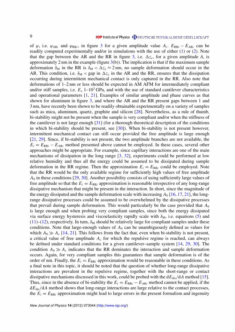
Figure 3. Experimental (a) phase and (b) amplitude curves shown as a functionof separation zc. The absolute value of zc is not known but from this work itcan be recovered. An appropriate choice of free amplitude is shown to allowacquiring the amplitude branches in both the attractive AR and the repulsiveRR regimes. The sample is aluminum. Experimental parameters: A0 ≈ 25 nm,k ≈ 2 N m−1, Q ≈ 150 and R ≈ 7 nm and a Cypher (Asylum Research) has beenused to acquire the data.

where m = k/ω2 and F0 is the drive force. The parameters used in the numerical integration arek = 40 N m−1, Q = 500, ω = 2p f0( f0 = 300 kHz), Et = 170 GPa (Young modulus of the tip),Es = 1 GPa (Young modulus of the sample), R = 7 nm, FAD = 1 nN, α = 0.5 and η = 500 Pa s.This choice of k allows us to consider the simplified form of 1dmi j , i.e. 1dmi j = 1zci j + 1z0i j −

1Aij, since the excitation of higher harmonics is then inhibited. The only unresolved stepbefore the above formalism, equations (26)–(32), can be employed relates to the decouplingof the energy dissipated during sample deformation Ei from the long-range dissipation. In thenumerical example in this work, the bi-stability in AM AFM is used to decouple the long- andshort-range dissipation. Bi-stability is a common phenomenon in ambient AFM [21, 30]. Inparticular, for a given critical value of free amplitude, i.e. A0 = Ac, two amplitude branches(low-amplitude branch or attractive regime AR and high-amplitude branch or repulsive regimeRR) can be recovered [14, 21] (see figure 3 for an experimental example). Assuming thatthe dissipative processes involved in long-range dissipation are captured in the AR (EARi)

and that the dissipation involved in sample deformation occurs in the RR only (ERRi), itfollows that for a given data point i or amplitude Ai , Ei = ERRi − EARi . Note the two values

New Journal of Physics 14 (2012) 073044 (http://www.njp.org/)

9

of ϕ, i.e. ϕARi and ϕRRi , in figure 3 for a given amplitude value Ai . ERRi − EARi can bereadily computed experimentally and/or in simulations with the use of either (1) or (2). Notethat the gap between the AR and the RR in figure 3, i.e. 1zc, for a given amplitude A, isapproximately 2 nm in the example (figure 3(b)). The implication is that if the maximum sampledeformation δM in the RR is δM < 1zc ≈ 2 nm, no sample deformation should occur in theAR. This condition, i.e. δM < gap in 1zc in the AR and the RR, ensures that the dissipationoccurring during intermittent mechanical contact is only captured in the RR. Also note thatdeformations of 1–2 nm or less should be expected in AM AFM for intermediately compliantand/or stiff samples, i.e. Es 1–103 GPa, and with the use of standard cantilever characteristicsand operational parameters [1, 21]. Examples of similar amplitude and phase curves as thatshown for aluminum in figure 3, and where the AR and the RR present gaps between 1 and3 nm, have recently been shown to be readily obtainable experimentally on a variety of samplessuch as mica, aluminum, quartz, graphite and silicon [28]. Nevertheless, as a rule of thumb,bi-stability might not be present when the sample is very compliant and/or when the stiffness ofthe cantilever is not large enough [31] (for a thorough theoretical description of the conditionsin which bi-stability should be present, see [30]). When bi-stability is not present however,intermittent mechanical contact can still occur provided the free amplitude is large enough[21, 29]. Since, if bi-stability is not present, the two amplitude branches are not available, theEi = ERRi − EARi method presented above cannot be employed. In these cases, several otherapproaches might be appropriate. For example, since capillary interactions are one of the mainmechanisms of dissipation in the long range [3, 32], experiments could be performed at lowrelative humidity and thus all the energy could be assumed to be dissipated during sampledeformation in the RR regime. Then the approximation Ei = ERRi could be employed. Notethat the RR would be the only available regime for sufficiently high values of free amplitudeA0 in these conditions [29, 30]. Another possibility consists of using sufficiently large values offree amplitude so that the Ei = ERRi approximation is reasonable irrespective of any long-rangedissipative mechanism that might be present in the interaction. In short, since the magnitude ofthe energy dissipated and the sample deformation scale with increasing A0 [16, 17, 21], the long-range dissipative processes could be assumed to be overwhelmed by the dissipative processesthat prevail during sample deformation. This would particularly be the case provided that A0

is large enough and when probing very compliant samples, since both the energy dissipatedvia surface energy hysteresis and viscoelasticity rapidly scale with δM, i.e. equations (5) and(11)–(12), respectively. In turn, δM should be relatively large for compliant samples under theseconditions. Note that large-enough values of A0 can be unambiguously defined as values forwhich A0 � Ac [14, 21]. This follows from the fact that, even when bi-stability is not present,a critical value of free amplitude Ac for which the repulsive regime is reached, can alwaysbe defined under standard conditions for a given cantilever–sample system [14, 29, 30]. Thecondition A0 � Ac indicates that the RR dominates the interaction and sample deformationoccurs. Again, for very compliant samples this guarantees that sample deformation is of theorder of nm. Finally, the Ei = ERRi approximation would be reasonable in these conditions. Asa final note in this topic, it should be noted that the question of whether long-range dissipativeinteractions are prevalent in the repulsive regime, together with the short-range or contactdissipative mechanisms discussed in this work, could be probed with the dEdis/dA method [15].Thus, since in the absence of bi-stability the Ei = ERRi − EARi method cannot be applied, if thedEdis/dA method shows that long-range interactions are large relative to the contact processes,the Ei = ERRi approximation might lead to large errors in the present formalism and ingenuity

New Journal of Physics 14 (2012) 073044 (http://www.njp.org/)

10

in the experimental approach would be required. In particular, note that the dEdis/dA methodshows how to identify contributions from interfacial long-range interaction which might beprevalent in several scenarios in AM AFM [1].

In the simulations of the example presented here, the condition Ei = ERRi − EARi can beemployed since bi-stability is present. In particular, the critical value of A0 in the example isA0 = Ac ≈ 9 nm (curve not shown). Moreover, the gap between force regimes, i.e. 1zc (seefigure 3(b) for an example), is of approximately 1–2 nm. As stated, if the maximum sampledeformation δM is less than this gap, i.e. if δM < 1–2 nm, both amplitude branches can berecovered with sample deformation only occurring in the RR as required. In the example inthe simulation, this condition is satisfied since the maximum sample deformation is less than1 nm (see below) agreeing with previous studies for Es 1–103 GPa [1]. Although only three datapoints are necessary to estimate the values of δM, η and α, several data points are used here inorder to establish the accuracy of the technique numerically. Furthermore, this does not restrictthe practicality of the method since, in experimental curves, a very large number of data pointscan be collected (see figure 3). In the numerical simulations, N = 21 data points have beenused. This leads to 1 + N (N − 3)/2 = 190 estimations for δM (32). Taking as the reference theunknown deformation δM at zc = 5.4 nm, the value δM = 0.6717 nm (mean value) is recoveredat zc = 5.4 nm with the use of (32). Note that, as stated, prior knowledge of the absolute valueof zc is not required to find δM. The standard deviation is ≈8 pm. The true value of δM atzc = 5.4 nm, according to numerical integration, is 0.6718 nm. The error is thus a fraction ofa pm. This demonstrates the potential accuracy of the method. Note that the Chauvenet rulehas been applied to the 190 values of K and only two values have been excluded as outliers.Errors are due to the assumptions in the derivation of Eη (12), the use of the simplified form of1dmi j (24) and the lack of accuracy in the numerical integration of the equation of motion (a stepsize of 4096 data points per cycle and a standard Runge–Kutta algorithm of the fourth order havebeen used in the numerical integration). Once δM is known, η and α can be recovered from (19)and (20). N (N − 1)/2 = 210 estimations for η and α can be computed. The recovered (mean)value for η is 503 Pa s with a standard deviation of 41 Pa s and where a single outlier has beenexcluded from the data set (32 estimations have been excluded from a physical point of viewsince these were negative). Recall the true value is η = 500 Pa s. For α the recovered (mean)value is 0.505 with a standard deviation of 1 (two outliers and 33 negative values excluded).Recall that the true value is α = 0.5. Finally, we note that three solutions for Ki j − Kik = 0 aretypically found for any three given data points i, j and k. Only one solution produces a realpositive deformation δM, where Ki j > 0.

This work shows that by monitoring the magnitude of the energy dissipated in thetip–sample interaction with sufficient accuracy and by correctly establishing the dissipativemechanisms during sample deformation, the tip–sample deformation can be recovered with,in principle, pm resolution. It has also been shown that fundamental dissipative properties ofthe sample can also be recovered quantitatively. In particular, viscoelasticity and surface energyhysteresis can be quantified. Experimentally, errors in the acquisition of amplitude A (partsper thousand [19, 33]) and the phase ϕ (fractions of degrees [4]) should be expected to affectthe accuracy of the method since the formalism developed here (equations (26)–(32)) dependson the accuracy in the measurements of these observables. As stated elsewhere [19], this isa general limitation of AM AFM methods. Other limitations include the calibration of otherotherwise known parameters such as the tip radius and the stiffness of the cantilever but thisis a field of research where developments are being made continuously [12, 14, 34]. More

New Journal of Physics 14 (2012) 073044 (http://www.njp.org/)

11

fundamentally, deeper insights into other dissipative channels such as the capillary interactionare being reported [18, 28, 35, 36] and these might imply that future developments of the theorypresented in this work will potentially increase the accuracy of the recovered parameters. As afinal note, it should be noted that dissipative properties might depend on nanoscale dimensions.In this respect, developments regarding the characterization and accurate calibration of thetip radius in situ [14] might be valuable in future experimental work and in relation to thepresent formalism. That is, by probing the sample with a range of tip radii, the dependenceor otherwise independence of dissipative properties on dimensions could be probed. This couldhave implications on a theory where the interface between atomic and macroscale phenomena isstudied. In summary, this work establishes a robust framework to quantify dissipative propertieswith true nanoscale resolution in ambient conditions.

References

[1] Garcia R, Gomez C J, Martinez N F, Patil S, Dietz C and Magerle R 2006 Identification of nanoscaledissipation processes by dynamic atomic force microscopy Phys. Rev. Lett. 97 016103

[2] Garcia R, Magerele R and Perez R 2007 Nanoscale compositional mapping with gentle forces Nature Mater.6 405–11

[3] Sahagun E, Garcıa-Mochales P, Sacha G M and Saenz J J 2007 Energy dissipation due to capillaryinteractions: hydrophobicity maps in force microscopy Phys. Rev. Lett. 98 176106

[4] Cleveland J P, Anczykowski B, Schmid A E and Elings V B 1998 Energy dissipation in tapping-mode atomicforce microscopy Appl. Phys. Lett. 72 2613–5

[5] Hoffmann P M, Jeffery S, Pethica J B, Ozgur Ozer H and Oral A 2001 Energy dissipation in atomic forcemicroscopy and atomic loss processes Phys. Rev. Lett. 87 265502

[6] Kawai S, Federici Canova F, Glatzel T, Foster A S and Meyer E 2011 Atomic-scale dissipation processes indynamic force spectroscopy Phys. Rev. B 84 115415

[7] Santos S, Gadelrab K R, Silvernail A, Armstrong P, Stefancich M and Chiesa M 2012 Energy dissipationdistributions and atomic dissipative processes in the nanoscale in dynamic atomic force microscopyNanotechnology 23 125401

[8] Liu Y H, Wang D, Nakajima K, Zhang W, Hirata A, Nishi T, Inoue A and Chen M W 2011 Characterizationof nanoscale mechanical heterogeneity in a metallic glass by dynamic force microscopy Phys. Rev. Lett.106 125504

[9] Tamayo J 1999 Energy dissipation in tapping-mode scanning force microscopy with low quality factors Appl.Phys. Lett. 75 3569–71

[10] Lozano J R and Garcia R 2008 Theory of multifrequency atomic force microscopy Phys. Rev. Lett.100 076102

[11] Payam A F, Ramos J R and Garcia R 2012 Molecular and nanoscale compositional contrast of soft matter inliquid: interplay between elastic and dissipative interactions ACS Nano 6 4663–70

[12] Sader J E, Chon J W M and Mulvaney P 1999 Calibration of rectangular atomic force microscope cantileversRev. Sci. Instrum. b 70 3967

[13] Hutter J L and Bechhoefer J 1993 Calibration of atomic force microscope tips Rev. Sci. Instrum. 64 1868–73[14] Santos S, Guang L, Souier T, Gadelrab K R, Chiesa M and Thomson N H 2012 A method to provide rapid

in situ determination of tip radius in dynamic atomic force microscopy Rev. Sci. Instrum. 83 043707[15] Gomez J C and Garcia R 2010 Determination and simulation of nanoscale energy dissipation processes in

amplitude modulation AFM Ultramicroscopy 110 626–33[16] Martinez N and Garcia R 2006 Measuring phase shifts and energy dissipation with amplitude modulation

atomic force microscopy Nanotechnology 17 S167–S72[17] Santos S and Thomson N H 2011 Energy dissipation in a dynamic nanoscale contact Appl. Phys. Lett.

98 013101

New Journal of Physics 14 (2012) 073044 (http://www.njp.org/)

12

[18] Choe H, Hong M-H, Seo Y, Lee K, Kim G, Cho Y, Ihm J and Jhe W 2005 Formation, manipulation, andelasticity measurement of a nanometric column of water molecules Phys. Rev. Lett. 95 187801

[19] Hu S and Raman A 2008 Inverting amplitude and phase to reconstruct tip–sample interaction forces in tappingmode atomic force microscopy Nanotechnology 19 375704

[20] Gadelrab K R, Santos S, Souier T and Chiesa M 2012 Disentangling viscous and hysteretic components indynamic nanoscale interactions J. Phys. D: Appl. Phys. 45 012002

[21] Santos S, Gadelrab K R, Souier T, Stefancich M and Chiesa M 2012 Quantifying dissipative contributions innanoscale interactions Nanoscale 4 792–800

[22] Forchheimer D, Platz D, Tholen E A and Haviland D B 2012 Model-based extraction of material propertiesin multifrequency atomic force microscopy Phys. Rev. B 85 195449

[23] Tamayo J and Garcia R 1996 Deformation, contact time, and phase contrast in tapping mode scanning forcemicroscopy Langmuir 12 4430–5

[24] Fischer-Cripps A C 2004 Nanoindentation (New York: Springer)[25] Martınez N F, Kaminski W, Gomez C J, Albonetti C, Biscarini F, Perez R and Garcıa R 2009 Molecular scale

energy dissipation in oligothiophene monolayers measured by dynamic force microscopy Nanotechnology20 434021

[26] Derjaguin B V, Muller V and Toporov Y 1975 Effect of contact deformations on the adhesion of particlesJ. Colloid Interface Sci. 53 314–26

[27] Santos S, Barcons V, Verdaguer A, Font J, Thomson N H and Chiesa M 2011 How localised are energydissipation processes in the nanoscale? Nanotechnology 22 345401

[28] Barcons V, Verdaguer A, Font J, Chiesa M and Santos S 2012 Nanoscale capillary interactions in dynamicatomic force microscopy J. Phys. Chem. C 16 7757–66

[29] Garcia R and San Paulo A 1999 Attractive and repulsive tip-sample interaction regimes in tapping modeatomic force microscopy Phys. Rev. B 60 4961–7

[30] San Paulo A and Garcia R 2002 Unifying theory of tapping-mode atomic force microscopy Phys. Rev. B66 041406

[31] Chen X, Davies M C, Roberts C J, Tendler S J B, Williams P M and Burnham N A 2000 Optimizing phaseimaging via dynamic force curves Surface Sci. 460 292–300

[32] Zitzler L, Herminghaus S and Mugele F 2002 Capillary forces in tapping mode atomic force microscopyPhys. Rev. B 66 155436

[33] Garcia R and Perez R 2002 Dynamic atomic force microscopy methods Surf. Sci. Rep. 47 197–301[34] Cleveland J, Manne S, Bocek D and Hansma P K 1993 A nondestructive method for determining the spring

constant of cantilevers for scanning force microscopy Rev. Sci. Instrum. 64 403–5[35] Szoszkiewicz R and Riedo E 2005 Nucleation time of nanoscale water bridges Phys. Rev. Lett. 95 135502–4[36] Santos S, Barcons V, Verdaguer A and Chiesa M 2011 Sub-harmonic excitation in AM AFM in the presence

of adsorbed water layers J. Appl. Phys. 110 114902

New Journal of Physics 14 (2012) 073044 (http://www.njp.org/)