QUANTIFICATION OF ESCHERICHIA COLI AND ENTEROCOCCILEVELS IN WET WEATHER AND DRY WEATHER FLOWS

Sumandeep Singh Shergill and Robert Pitt Dept. of Civil and Environmental Engineering

University of Alabama Tuscaloosa, AL 35487

ABSTRACT

Forty percent of rivers, 45% of lakes and 50% of estuaries assessed by the National Water Quality Inventory (2000) were not clean enough to support designated fishing and swimming uses. Pathogens were found to be one of the leading causes of impairments in these waters. Urban runoff is recognized as a leading source of organisms potentially indicating the presence of pathogens. Urban runoff can be defined as any discharge from a separate storm drainage system. Urban runoff traditionally had been defined to include precipitation and wash off from lawns and other landscaped areas, buildings, roadways and parking lots. However, other flows may enter the storm drainage system from such sources as infiltrating groundwater, leaking domestic water supplies and sewage, washwaters, and other inappropriate entries to the storm drainage system. This research was conducted to quantify the levels of indicator bacteria, and their sources, in urban areas. The main objective of this research was to identify possible sources of E. coli and enterococci bacteria in dry and wet-weather flows in storm drainage systems.

An urban area consists of many different kinds of land uses such as residential, institutional, commercial, industrial open spaces, etc. Each type of land use consists of various types of source areas, such as roofs, parking lots, landscaped areas, playgrounds, driveways, undeveloped areas, sidewalks. Four representative source area types were sampled during this research; including rooftops, parking lots, open spaces, and streets. Two parallel sites were sampled for each source area type; one affected by birds and other animals, and another set with less influence from birds and other animals. A section of Cribbs Mill Creek in Tuscaloosa, Alabama, was also selected for dry weather sampling at outfalls. The section of the creek was selected such that the drainage areas contributing to outfalls had either commercial or residential land uses. Potential inappropriate discharge water samples were also obtained, including influent samples from the Tuscaloosa sewage treatment plant, local springs, irrigation runoff water, domestic water taps, car wash, and laundry water. Overall, total coliforms, E. coli and enterococci bacterial analyses were conducted on 202 wet weather and 278 dry weather flow water samples. All samples were analyzed using IDEXX Quantitray enumeration procedures.

E. coli and enterococci levels larger than 2,400 and 24,000 MPN/100 mL, respectively, were observed in wet weather samples collected from various source areas which could not possibly be contaminated with sanitary sewage. The levels of indicator bacteria present in the urban runoff source area samples exceeded the EPA 1986 single sample maximum value water quality criteria in 31% of the samples for E. coli and in 74% of the samples for enterococci. The geometric mean criteria were exceeded in 100% of the source area samples. Since both the indicator organisms studied (E. coli. and enterococci) only originate in intestines of warm­

blooded animals, birds and other urban animals can be considered important sources of bacteria in stormwater.

This assumption was tested by conducted additional monitoring. Comparisons of samples collected from areas prone to urban animal use and those that are not, showed that large overlaps exist between the bacterial concentrations found from both types of areas. Bacterial levels from roofs prone to urban animal use (squirrels and birds) were significantly higher than from roofs not exposed to such use. The other source areas did not show any significant differences in bacterial levels between areas prone and not prone to urban animal use, except for some street areas. This could be the result of a combination of factors, such as the persistence of bacteria in soil, the inadvertent contamination by runoff from other areas frequented by animals, the mobility of small urban animals, or the ubiquitous presence of moderate levels of these organisms in most urban areas. Statistical analyses problems were also caused by periodic very high bacteria values that exceeded the range of the experiments.

A further objective of this study was to find how E. coli and enterococci could be effectively used to identifying the presence of inappropriate sanitary sewage in storm drainage systems during dry weather. Many stormwater system managers believe that the presence of indicator bacteria exceeding regulatory levels indicates the likely presence of sanitary sewage. During this study, sewage samples were compared with wet weather and dry weather source area samples (from the project reference sample library). The probability of the sewage and source area sample bacteria levels being significantly different was determined using the Mann Whitney test. When the values of the probabilities were ≤ 0.05, the diluted sewage sample bacteria levels were determined to be significantly higher as compared to bacterial levels in other source area samples (with a 1 in 20 error level). It was found that the dry-weather outfall samples showing E. coli and enterococci levels higher than 12,000 MPN/100 mL and 5,000 MPN/100 mL respectively, are likely contaminated by sanitary sewage. Levels lower than this can be caused by other sources, such as irrigation runoff, carwash water, or laundry water.

Other findings of this research included:

• Bacteria levels in urban areas are not source limited, i.e. measured bacteria levels did not decrease with increasing amounts of rain, or even with increasing rain intensities. The levels may increase, or decrease, somewhat with time, but stayed generally level. • Seasons having low temperatures are associated with decreased bacterial levels. • The ratio of E. coli /enterococci was not constant and varied greatly for all conditions. • Wet weather samples had mostly higher enterococci levels than E. coli, while dry weather source area samples (such as springs and irrigation runoff) had higher E. coli levels than enterococci levels. • Both the indicators followed the same general trend for every site; i.e. both E. coli and enterococci levels increased or decreased simultaneously, although by different amounts. • Sewage samples need vigorous agitation before analyses to break up the lumps of fecal matter in which bacteria are present. • Samples must be kept refrigerated and analyzed shortly after sample collection. Samples a day old and unrefrigerated can be expected to have decreased bacteria levels compared to chilled and fresh samples.

This research was funded as part of a 104(b)3 grant from the U.S. Environmental Protection Agency (Bryan Rittenhouse was the project officer) to the Center for Watershed Protection (under the project management of Ted Brown and Tom Schueler) in 2001. The University of Alabama was a subcontractor to the Center. Sumandeep Shergill conducted much of the research reported in this paper, with the assistance of other graduate students at UA, and his master’s thesis reporting this work was accepted by the University in May of 2004.

METHODOLOGY

In order to achieve the objectives of this research, microbial analyses were conducted on 202 wet weather and 278 dry weather samples. Both E. coli and enterococci analyses were conducted. Total coliforms were also evaluated as part of the E. coli tests. The following tasks were accomplished during this research:

• Effects of Urban Wildlife on Stormwater Bacteria Levels. Four source areas were selected for sampling. For each category of source area, two sites were selected, prone and not prone to urban animal use. The prone locations were those where urban wildlife (birds and squirrels for roofs, and dogs for ground-level surfaces) use is common and not prone locations where urban wildlife appears to be generally absent. The number of samples collected in each category during this part of the research is listed in Table 1.

Table 1. Total Number of Sample Pairs Collected From Each Source Area Site No. of Paired Samples

Open space- Prone 11 Open space- Not prone 10

Parking lot – Prone 13 Parking lot- Not Prone 10

Roof - Prone 12 Roof - Not Prone 12 Streets- Prone 10

Streets- Not Prone 10

In a few cases, the number of samples from one site analyzed for E. coli was different from that of enterococci. A total of 176 samples were analyzed.

• Seasonal Variations. The climate of Tuscaloosa, Alabama, is subtropical with four distinct seasons including winter (December through February), spring (March and April), summer (May through September) and autumn (October and November). Anticipating that bacterial levels would vary with season, an attempt was made to take samples in every season. Wet weather sampling was conducted from August 2002 to June 2003. No samples were collected during the months of December and March. This objective was to compare cold months (December through February, generally having temperatures below 50o F) with samples collected during the warmer months.

• Variations within Storms. Additional tests were also conducted to determine the potential causes for the large variability found during the bacterial analyses of the sheetflow samples. During a single storm on 25 September 2002, all the sites were sampled twice, once in the

morning and then again in the evening. In addition, six samples from two source areas were collected at intervals of 15 to 30 minutes during a single storm on 17 October 2003. A total of 24 samples were analyzed for these tests.

• Effect of Sample Handling. Three factors involving sample handling were also studied. These included holding time, refrigeration, and vigorous sample shaking. For these tests, a single 5 liter sample was taken from one source area from which 100 mL sub samples were tested after 1, 2, 5, 9, 24, and 48 hrs. The 5 liter sample was split into two components, one was refrigerated, and the other was not. The effect of refrigeration over one to two days was also measured. The effect of shaking was measured by withdrawing an initial 100 mL sample from the unshaken sample bottles, and then shaking the sample bottles and testing another 100 mL sample.

• Reference Sample Collection (Library Samples). 12 samples were collected from each of several source areas: the influent to a sewage treatment plant, local springs, irrigation runoff, domestic water taps, car wash, typical local industry, and laundry water. Sewage samples were compared with other reference samples and wet weather samples. A total of 142 samples were analyzed.

• Outfall Sample Collection. A five mile stretch of Cribbs Mill Creek in Tuscaloosa, Alabama, was selected for dry weather sampling to test methods to detect inappropriate discharges to the creek. A total of 77 total outfalls were examined and bacterial analyses were conducted during three different periods from outfalls having dry weather flows. A total of 136 samples were analyzed during this test phase.

Sampling Procedures Wet weather sampling started in August 2002 and was completed in June 2003. The objective was to represent all the seasons so that effects of season on bacterial concentrations could be examined. Samples were taken during rains once or twice a month during this period, except for December 2002 and March 2003 when no samples were obtained. Dry weather sampling involved collection of Tuscaloosa source area samples for preparing the Tuscaloosa source area reference sample library. Most of the library samples were collected during the months of May and June 2003. All samples were analyzed using the IDEXX Quantitray enumeration procedure. All samples were analyzed for total coliforms, E. coli and enterococci. Although dry weather samples were analyzed for various other constituents, this paper only presents results for the microbial analyses. The quality assurance /quality control (QA/QC) procedures followed are described later.

• Wet Weather Sampling Procedure. Samples were collected according to procedures given in Standard Methods for the Examination of Water and Wastewater (Standard Methods-20th

edition, 1998) for microbiological examination. Sterile techniques were used to avoid sample contamination. Sterile gloves were worn during sampling and analysis, and the samples were collected in presterilized 100 mL plastic bottles supplied by IDEXX . The bottles contain sodium thiosulphate (Na2S203 ) to prevent problems with chlorine in the samples. Na2S203 is a dechlorinating agent that neutralizes any residual halogen and prevents continuation of bacterial disinfection during sample transit. The use of Na2S203 more accurately results in the true microbial content of the water at the time of sampling (Standard Methods-20th edition, 1998).

All samples were taken manually. The sample bottles were filled up to the 100 mL mark, leaving ample air space to facilitate mixing by shaking, before testing. The pre-sterilized sample bottles were filled without rinsing and care was taken so that the inner surface of stopper or cap did not become contaminated. The bottle cap was replaced immediately.

The sample bottle labels listed the date, sample I.D, and time of sampling, using waterproof markers. The sample bottles had labels on both the cap and the bottle, preventing the caps form being interchanged. Filled sample bottles were then put in a backpack for transporting to the lab. During the initial five sampling rounds, no sample dilutions were made, so two sample bottles per site (one for E. coli and other for enterococci) were taken. From the sixth round on, three 100 mL samples were taken per site to allow for dilution and an expanded range of MPN values.

Sampling was conducted in a random order for each event to make sure that all the sites were visited an approximately equal number of times. Before leaving for the field, the rain conditions and forecast were checked using Internet weather satellite images and forecasts, and local rain gages, to help ensure that sufficient rain would fall to produce sheetflow. It is almost impossible to obtain satisfactory samples during light rains. The time at which the sample was obtained at a particular site was noted on the sample bottle label right before sampling.

Rooftop samples were obtained by placing the sample bottle directly under the downspout. The bottle was removed soon before it filled to the 100 mL mark. The bottle cap was then used to fill the sample bottle exactly to the 100mL mark. Sheetflow samples were taken from parking lots and streets. The sampling locations on the street or parking lots were selected so that runoff was not mixed with runoff from other source areas. Similarly, sampling places inside the parking lots were selected such that there was minimal mixing from other source areas. Samples were taken by holding the sample bottle near its base, keeping it tilted at an angle with mouth facing downstream. Sheetflow samples were placed into the bottle with the cap from the bottle. Care was taken not to scratch the pavement surface with the cap during sampling. It was difficult to collect sheetflow samples from open spaces. Most open space samples were obtained from ponded water.

Samples collected from different sites were kept in different Zip Lock bags, put in the backpack and transported to the laboratory. Microbiological analysis of the water samples was started as soon as possible after collection to avoid changes in the microbial population.

• Dry Weather Sampling Procedure. Cribbs Mill Creek in Tuscaloosa, Alabama, was selected for dry weather sampling. Its’ watershed contains residential, commercial, open space land use areas. Other favorable characteristics were moderate flow, accessibility by road, and it was in a completely urbanized area that has been long developed. A five-mile section of the creek was selected for sampling.

The equipment taken to the field included

• One liter HDPE sample bottles • 100 mL pre-sterilized sample bottles supplied by IDEXX

• Non-mercury thermometer for onsite temperature measurement • GPS unit to record locations of outfalls • Reinforced (snake-proof) neoprene waders • Spray paint for labeling outfalls • Outfall characterization form • Street map of area • First aid kit • Walkie talkie • A dipper to sample inaccessible outfalls • Digital camera • Duct tape and a permanent marker • Ice cooler with ice packs to preserve the samples

Before sampling during any day, the field crew contacted the local Tuscaloosa Police Department to let them know the area of creek being investigated that day. The field crew consisted of three people. Upon arriving at the first site, two people waded the creek in a downstream direction carrying the field equipment in backpacks, while one person with a street map, cooler (with coolant), and a walkie-talkie drove the vehicle to a convenient downstream location where the creek intersects the street. Collected samples were placed in a portable ice cooler in the vehicle after each stretch was sampled. This collection point was usually about a half mile downstream from the last collection point. About 5 or 6 samples are usually collected from each stretch of creek and iced within a half hour of collection. Heavy-duty waders were always worn while wading which provided protected from debris (broken glass and other sharp debris, bricks etc.) and certain wildlife species (rattlesnakes, cottonmouth, etc.).

The first two creek walks involved a greater effort and time to complete because of the need to locate the outfall locations. After three complete creek walks, no new outfalls were found, and the field time was appreciably shortened. A total of 77 outfalls were eventually found in the initial study reach. Outfalls were numbered using black spray paint. The average distance between the outfalls was about 50 feet, and about six flowing outfalls were sampled during a days creek walk. About 5 to 7 days were needed for every creek walk, or about one mile per day. Out of 77 total outfalls, 20-25 were flowing during every creek walk. When a branch enters the main creek, the sampling crew went to the origin of the branch and walked downstream marking outfalls along the way. All sorts of outfalls were found, including open ditches, concrete outfalls, ductile iron pipe outfalls, and PVC outfalls. A few only drained the adjacent paved parking areas, while most were conventional outfalls draining 5 to 50 acres each. The following URL includes a large aerial photograph showing all outfalls, along with individual outfall photographs: http://www.eng.ua.edu/~rpitt/Research/ID/ID2.shtml

During the last three creek walks, bacterial analyses were also conducted, requiring two 100 mL samples collected for each flowing outfall, in addition to the 1L sample.

The following steps were followed at every outfall:

1) If not already marked, the outfall number was painted on the outfall 2) One 1L sample and two 100 mL grab samples were taken for each flowing outfall.

3) The water temperature was measured from the 1L sample bottle. 4) If not already recorded, the latitude and longitude were noted from the GPS. 5) The field characterization forms were filled out for each outfall visit. 6) Photographs of the outfall were taken.

After the third creek walk, some branches of the creek were dropped from further evaluations because of time and a redundancy of the residential land uses in which the branches were located. The dry weather sampling was conducted at least 24 to 48 hrs after rains, depending upon the rain depths. Samples were collected in the morning and refrigerated, while the 100 mL samples that were collected for bacterial analyses were analyzed immediately after arriving at the lab after each morning sample collection. All the other constituents were usually analyzed that same afternoon. Other constituents analyzed were ammonia, boron, color, conductivity, detergents, fluorescence, fluoride, hardness, potassium, pH, optical brighteners, and turbidity.

• Library (Reference) Sample Collection Procedure. All the library samples were collected in 1 L HDPE bottles and pre-sterilized 100 mL sample bottles. Tap water samples were collected from a service pipe directly connected with the main, not from a cistern or storage tank. The tap water was allowed to flow fully for two to three minutes for clearing the service line and then the sample was taken. It was difficult to collect samples directly from the springs, as the water flow was very slow (dripping). New clean zip lock bags were used to collect samples from the Jack Warner Parkway Spring (near old sealed coal mines under the campus). Samples from Mars Spring were collected with a dipper sampler.

Car wash samples were collected as sheetflow flowing from the washing of the cars. Laundry samples were taken from the washing machine directly when the washing cycle was about to finish and before the rinsing started. Sewage samples were taken from the automatic composite sampler located at the influent of the Tuscaloosa WWTP. Sewage samples collected immediately after rainy days were considered wet weather samples.

All the industries that were analyzed send water samples to the Tuscaloosa WWTP weekly for analyses as part of the local industrial pre-treatment program. Our library samples were obtained when these industrial samples were delivered to the treatment plant lab.

Irrigation water samples were mostly sheetflow water collected from the sidewalks or roads, which flowed due to over-watering of lawns. Some samples were collected from small depressions in the lawn itself and not from runoff after flowing across concrete.

Sample Analysis Procedures All the samples were analyzed for total coliforms, E. coli, and enterococci using EPA-approved IDEXX Laboratories methods. EPA suggested water quality criteria based upon E. coli and enterococci measurements in 1986. The IDEXX methods used were developed in response to these EPA microbiological guidelines. All the equipment and supplies needed were obtained from IDEXX, including Colilert or Colilert-18 reagent, Enterolert reagent, presterlized 100 mL sample bottles, Quanti-tray-2000 sample containers, Quanti-tray sealer, rubber insert pads, two incubators, two thermometers, comparartor, and a 6 watt, 365nm wavelength UV lamp. Figure 1

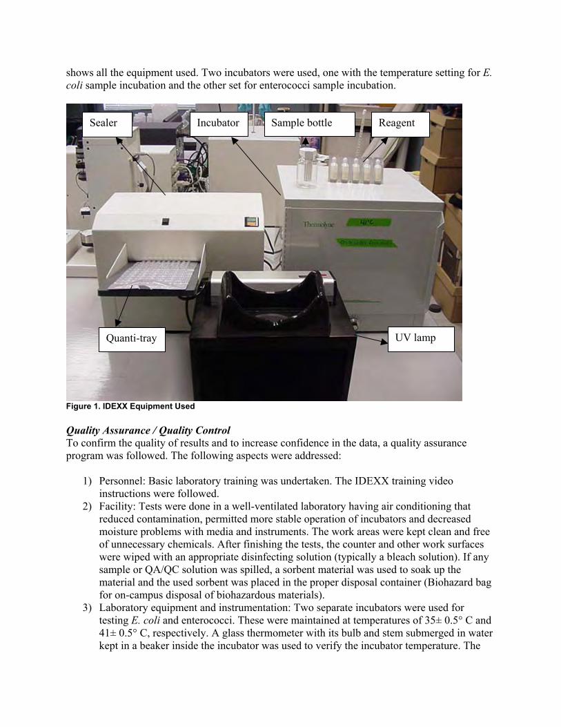
shows all the equipment used. Two incubators were used, one with the temperature setting for E. coli sample incubation and the other set for enterococci sample incubation.

Figure 1. IDEXX Equipment Used

ReagentSealer Incubator Sample bottle

UV lamp Quanti-tray

Quality Assurance / Quality Control To confirm the quality of results and to increase confidence in the data, a quality assurance program was followed. The following aspects were addressed:

1) Personnel: Basic laboratory training was undertaken. The IDEXX training video instructions were followed.

2) Facility: Tests were done in a well-ventilated laboratory having air conditioning that reduced contamination, permitted more stable operation of incubators and decreased moisture problems with media and instruments. The work areas were kept clean and free of unnecessary chemicals. After finishing the tests, the counter and other work surfaces were wiped with an appropriate disinfecting solution (typically a bleach solution). If any sample or QA/QC solution was spilled, a sorbent material was used to soak up the material and the used sorbent was placed in the proper disposal container (Biohazard bag for on-campus disposal of biohazardous materials).

3) Laboratory equipment and instrumentation: Two separate incubators were used for testing E. coli and enterococci. These were maintained at temperatures of 35± 0.5° C and 41± 0.5° C, respectively. A glass thermometer with its bulb and stem submerged in water kept in a beaker inside the incubator was used to verify the incubator temperature. The

water levels in the beakers were periodically checked to ensure that the bulb and stem of the thermometers were always submerged. The UV lamp and sealer were switched off after each use and were periodically cleaned.

4) Supplies: Supplies used for testing were Colilert and Colilert-18 reagent, Enterolert reagent; Quanti-cult bacterial cultures used for quality control, Quanti-trays, and 100 mL pre-sterilized sample bottles. The Quanti-cult and analytical reagents were stored in a refrigerator according to the manufacturer requirements. Quanti-trays and sample bottles supplied by IDEXX were sterile (certified by IDEXX) and disposable. This eliminates the use of glassware and any chances of contamination.

5) Analytic methods: The test used for total coliforms and E. coli, was the commercially available microbiological method included in Standard Methods for the Examination of Water and Wastewater, 20th edition (section 9223 B). Enterolert is an official ASTM method (#D6503-99). These methods are commonly used by many agencies, including the Alabama Department of Environmental Management (ADEM).

6) Analytical Quality control procedures: Every batch of Colilert and Colilert-18 reagent was checked by testing with known positive and negative control cultures (Quanti-cult®). Quanti-cult® is a set of ready to use bacterial cultures supplied by IDEXX. It consists of three sets each of three different bacterial cultures. Each set consists of 1-50 bacterial cells which were preserved in the colorless cap of a plastic vial. The contents of Quanti-cult® were kept stored in a refrigerator until time of use. Following are the contents:

• 3 E. coli capped vials labeled “EC” in foil packs and 2 reusable labels • 3 Klebsiella pneumoniae –capped vials labeled “KP” in foil packs and 2 reusable

labels. This is a total coliform bacterium. • 3 Pseudomonas aeruginosa – capped vials labeled “PA” in foil packs and 2

reusable labels. This is a non-coliform bacterium. • 12 rehydration fluid vials • 1 autoclavable foam vial holder

Quality control tests were run three times on different batches. All test results were acceptable and full results are reported by Shergill (2004).

RESULTS AND DISCUSSION

This section presents the results of the wet weather and dry weather sampling and bacteria analyses. Summary tables only are included here, with detailed results provided by Shergill (2004). Statistical analyses were conducted using MINITAB, EXCEL and Pro-Stat software.

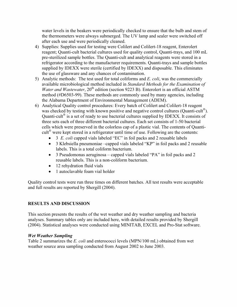
Wet Weather Sampling Table 2 summarizes the E. coli and enterococci levels (MPN/100 mL) obtained from wet weather source area sampling conducted from August 2002 to June 2003.

Table 2. Wet Weather Source Area Sampling Results

Sample I.D Date Sample Taken E. coli

(MPN/100 mL***) Enterococci

(MPN/100 mL) 21-Sep-02

OPEN SPACE -Prone* 25-Sep-02 25-Sep-02

10-Oct-02 27-Oct-02 5-Nov-02 29-Jan-03

6-Feb-03 6-Feb-03 24-Apr-03 14-May-03

12-Jun-03 27-Jun-03

1732.9 15.5 41.3

Not Sampled Not Sampled

2419.2 35.4

1 1

82 52

>2419.2 3.1

>2419.2 >2419.2 >2419.2

Not Sampled Not Sampled

19863 216 395

Not Sampled 322 2489

>24192 4106

21-Sep-02 OPEN SPACE– Not Prone** 25-Sep-02

25-Sep-02 10-Oct-02 27-Oct-02

15-Oct-02 5-Nov-02 29-Jan-03

6-Feb-03 24-Apr-03 14-May-03

12-Jun-03 27-Jun-03

Not Sampled 2419.2 866.4

Not Sampled Not Sampled

217.8 44.8 17.7

2 8.6

307.6 63.1 6.2

Not Sampled >2419.2 >2419.2

Not Sampled Not Sampled

>2419.2 8664 195 505

2755 9804

>24192 >24192

25-Sep-02 PARKING LOT- Not Prone 25-Sep-02

10-Oct-02 27-Oct-02

5-Nov-02 29-Jan-03

6-Feb-03 24-Apr-03 14-May-03

12-Jun-03 27-Jun-03

83.9 69.7 14.2

1553.1 15.8 4.1 <1

72.3 25.6

Not Sampled 5.2

>2419.2 2419.2

>2419.2 48.2 238 238 31

9804 1130

Not Sampled 613

21-Sep-02 PARKING LOT- Prone 25-Sep-02

25-Sep-02 10-Oct-02 27-Oct-02

5-Nov-02 29-Jan-03 29-Jan-03 29-Jan-03

6-Feb-03 24-Apr-03 14-May-03

12-Jun-03 27-Jun-03

1046.2 137.6 66.3 980.4 866.4 17.3 52

54.6 37.3 6.3 8.3

290.9 Not Sampled

29.5

529.8 >2419.2

344.8 >2419.2 >2419.2

158 199 160 145 150 127 805

Not Sampled 416

29-Aug-02 ROOF- Prone 21-Sep-02

25-Sep-02 25-Sep-02 10-Oct-02 27-Oct-02

5-Nov-02 29-Jan-03

6-Feb-03 24-Apr-03

14-May-03 12-Jun-03 27-Jun-03

145.5 461.1 18.7

1413.6 410.6

>2419.2 >2419.2

2 <1

517.2 Not Sampled

727 2419.2

Not Sampled >2419.2 >2419.2

980.4 67.9

1 9.3 16.4 31

>24192 Not Sampled

24192 15531

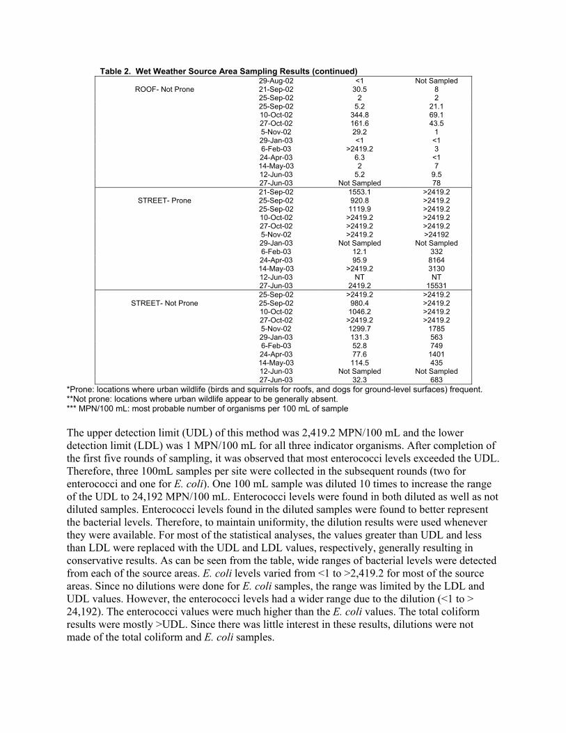
Table 2. Wet Weather Source Area Sampling Results (continued) 29-Aug-02 <1

ROOF- Not Prone 21-Sep-02 30.5 25-Sep-02 2 25-Sep-02 5.2 10-Oct-02 344.8 27-Oct-02 161.6

5-Nov-02 29.2 29-Jan-03 <1

6-Feb-03 >2419.2 24-Apr-03 6.3 14-May-03 2

12-Jun-03 5.2 27-Jun-03 Not Sampled

Not Sampled 8 2

21.1 69.1 43.5

1 <1 3

<1 7

9.5 78

21-Sep-02 1553.1 STREET- Prone 25-Sep-02 920.8

25-Sep-02 1119.9 10-Oct-02 >2419.2 27-Oct-02 >2419.2 5-Nov-02 >2419.2 29-Jan-03 Not Sampled

6-Feb-03 12.1 24-Apr-03 95.9 14-May-03 >2419.2

12-Jun-03 NT 27-Jun-03 2419.2

>2419.2 >2419.2 >2419.2 >2419.2 >2419.2 >24192

Not Sampled 332

8164 3130 NT

15531 25-Sep-02 >2419.2

STREET- Not Prone 25-Sep-02 980.4 10-Oct-02 1046.2 27-Oct-02 >2419.2

5-Nov-02 1299.7 29-Jan-03 131.3

6-Feb-03 52.8 24-Apr-03 77.6 14-May-03 114.5

12-Jun-03 Not Sampled 27-Jun-03 32.3

>2419.2 >2419.2 >2419.2 >2419.2

1785 563 749

1401 435

Not Sampled 683

*Prone: locations where urban wildlife (birds and squirrels for roofs, and dogs for ground-level surfaces) frequent. **Not prone: locations where urban wildlife appear to be generally absent.*** MPN/100 mL: most probable number of organisms per 100 mL of sample

The upper detection limit (UDL) of this method was 2,419.2 MPN/100 mL and the lower detection limit (LDL) was 1 MPN/100 mL for all three indicator organisms. After completion of the first five rounds of sampling, it was observed that most enterococci levels exceeded the UDL. Therefore, three 100mL samples per site were collected in the subsequent rounds (two for enterococci and one for E. coli). One 100 mL sample was diluted 10 times to increase the range of the UDL to 24,192 MPN/100 mL. Enterococci levels were found in both diluted as well as not diluted samples. Enterococci levels found in the diluted samples were found to better represent the bacterial levels. Therefore, to maintain uniformity, the dilution results were used whenever they were available. For most of the statistical analyses, the values greater than UDL and less than LDL were replaced with the UDL and LDL values, respectively, generally resulting in conservative results. As can be seen from the table, wide ranges of bacterial levels were detected from each of the source areas. E. coli levels varied from <1 to >2,419.2 for most of the source areas. Since no dilutions were done for E. coli samples, the range was limited by the LDL and UDL values. However, the enterococci levels had a wider range due to the dilution (<1 to > 24,192). The enterococci values were much higher than the E. coli values. The total coliform results were mostly >UDL. Since there was little interest in these results, dilutions were not made of the total coliform and E. coli samples.

Dry Weather Sampling Results Another component of this research included bacterial analyses of dry weather samples taken from outfalls flowing into Cribbs Mill Creek in Tuscaloosa, AL. Although the samples were analyzed for a number of parameters (as part of the EPA-funded Inappropriate Discharge Detection and Elimination “IDDE” project) this paper focuses on the bacterial analyses, i.e. E. coli and enterococci.

The “library” samples (reference samples) collected from various source areas were analyzed for various tracer materials, including E. coli and enterococci. This included samples from influent to sewage treatment plants, local springs, irrigation runoff, domestic water taps, car wash, and laundry water. Tables 3 and 4 show the results of the bacterial analyses of the library samples.

Statistical Analysis and Discussion • Wet Weather Data. Statistical analyses of wet weather flow data were conducted using MINITAB, ProStat, and MS-Excel. Although total coliforms were also detected (as part of the E. coli analyses), only E. coli and enterococci data were analyzed. Most of the total coliform observations were greater than the upper detection limit, and additional dilution analyses were not warranted for this secondary parameter. Observations from each of the source areas prone to urban animals were compared to observations from similar source areas not prone to urban animal use.

Table 3. E. coli Levels in Reference Samples (MPN/100 mL) Sewage Sewage

Sample Tap Spring (Dry (Wet No. Water Water Irrigation Laundry Carwash Industrial Weather)** Weather)

NO.1 NA 4.1 27.8 NA 1,553.1 66.3 >2,419.2 NO.2 NA 1 8.3 NA 1,413.6 >2,419.2 NA NO.3 NA NA >2,419.2 <1 4.1 0 >2,419.2 NO.4 NA NA >2,419.2 <1 14.6 3 816.4 NO.5 NA NA 31.8 <1 >2,419.2 NA NA NO.6 <1 <1 >2,419.2 >2,419.2 1,413.6 NA 12,033,000 NO.7 <1 290.9 >2,419.2 20.1 15.8 NA 2,851,000 NO.8 <1 172.3 >2,419.2 <1 11.9 NA 3,654,000 NO.9 <1 <1 >2,419.2 19.7 235.9 <1 2,187,000

NO.10 <1 9.7 1,299.7 <1 15.5 >2,419.2 1,785,000 NO.11 <1 1 >4,838.4 <1 1,553.1 <1 3,255,000 NO.12 <1 <1 >4,838.4 <1 <1 <1 2,282,000

Geometric mean* 1 5 771 3.9 94 19.7 15,484 2,590,319

Median <1 1 >2,419 <1 125 2 2,419 2,566,500 COV* 0 1.96 0.76 3.09 1.21 1.81 1.99 0.26

* Values calculated by replacing <1 with 1 and >2,419.2 with 2,419.2 ** The initial dry weather sewage samples were not well shaken before analyses and are therefore considered artificially low. The wet weather sewage samples were therefore used during this research to represent local sanitary sewage.

Table 4. Enterococci Levels in Reference Samples (MPN/100 mL) Sewage Sewage

Sample Tap Spring (Dry (Wet No. Water Water Irrigation Laundry Carwash Industrial Weather)** Weather) NO.1 NA 4.1 >2,419.2 NA >2,419.2 0 >2,419.2 NO.2 NA 36.4 2 NA 6.20 >2,419.2 NA NO.3 NA NA >2,419.2 <1 5.2 0 >2,419.2 NO.4 NA NA >2,419.2 <1 3.1 >2,419.2 43.6 NO.5 NA NA >2,419.2 <1 1 NA NA NO.6 <1 <1 287.7 <1 >2,419.2 NA 613,000 NO.7 <1 412 >2,419.2 <1 <1 NA 833,000 NO.8 <1 140.8 >2,419.2 <1 11.1 NA 598,000 NO.9 <1 3.1 >2,419.2 <1 <1 <1 292,000 NO.10 <1 65.7 >2,419.2 <1 <1 866.4 328,000 NO.11 <1 <1 >4,838.4 <1 2,419.2 22.2 369,000 NO.12 <1 <1 >4,838.4 <1 <1 <1 609,000 Geometric mean* 1 10.7 1,258 1 13 69 3,536 469,578 Median <1 4.1 >2,419 <1 4.2 12 >2,419 483,500 COV* 0 1.82 0.57 0 1.79 1.52 1.97 0.41

* Values calculated by replacing <1 by 1 and >2419.2 by 2419.2 ** The initial dry weather sewage samples were not well shaken before analyses and are therefore considered artificially low. The wet weather sewage samples were therefore used during this research to represent local sanitary sewage.

Due to the presence of large numbers of non-detected values, three types of paired and unpaired statistical tests were used to determine if significant differences occurred between the sites. MINITAB was used to plot box plots. For both, E. coli and enterococci, two separate box plots were prepared, one for warm months and the other for the whole year. Figures 2 and 3 show these box plots contrasting the observations from the sites. The box plots show the normal range box, extreme value symbols (stars) and the median symbols (circle). In order to prepare undistorted plots, values less than the lower detection limit (<1) were replaced by 0.5, and values greater than the upper detection limit values (>2,419.2) were removed. The number of observations greater than the UDL removed for each site is noted at the bottom of box plot.

As is common for most wet-weather bacteria observations, overlaps exist between different sampled categories. Larger overlaps require additional data to distinguish the data sets. The overlapping values observed for the sites prone and not prone to urban wildlife made it difficult to confirm if the sites had significantly different bacteria levels. Roof and street areas obviously had the largest differences, as shown on these figures.

The plots were supplemented with statistical tests to measure the significance of the likely differences between paired data sets. Kruskal Wallis tests were conducted, with values greater than UDL and less than LDL values were replaced by UDL and LDL values. The Kruskal-Wallis test performs a hypothesis test of the equality of the population medians for a one-way design (two or more populations). This test is a generalization of the procedure used by the Mann-Whitney test and offers a nonparametric alternative to the one-way analysis of variance (ANOVA). The Kruskal-Wallis test looks for differences among the population medians. The Kruskal-Wallis hypotheses are:

H0: the population medians are all equal versus H1: the medians are not all equal

Figure 2. Group Box Plot for E. coli for all Warm Months* *No. of values >2,419.2 removed: Roof- P: 2; Street-P: 4; Street- NP: 2

Figure 3. Group Box Plot for Enterococci for all Warm Months * * No. of values >2,419.2 removed: Roof- P- 3, Street-P-6 , Street- NP- 4, Parking lot -P- 3, Parking lot -NP- 2, Open space- P- 4 and Open space- NP-5

An assumption for this test is that the samples from the different populations are independent random samples from continuous distributions, with the distributions having the same shape. The

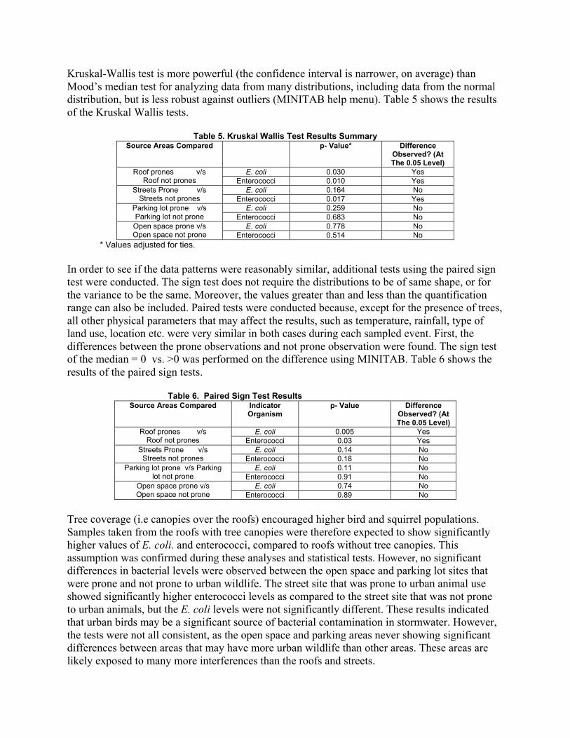
Kruskal-Wallis test is more powerful (the confidence interval is narrower, on average) than Mood’s median test for analyzing data from many distributions, including data from the normal distribution, but is less robust against outliers (MINITAB help menu). Table 5 shows the results of the Kruskal Wallis tests.

Table 5. Kruskal Wallis Test Results Summary Source Areas Compared p- Value* Difference

Observed? (At The 0.05 Level)

Roof prones v/s E. coli 0.030 Yes Roof not prones Enterococci 0.010 Yes

Streets Prone v/s E. coli 0.164 No Streets not prones Enterococci 0.017 Yes

Parking lot prone v/s E. coli 0.259 No Parking lot not prone Enterococci 0.683 No

Open space prone v/s E. coli 0.778 No Open space not prone Enterococci 0.514 No

* Values adjusted for ties.

In order to see if the data patterns were reasonably similar, additional tests using the paired sign test were conducted. The sign test does not require the distributions to be of same shape, or for the variance to be the same. Moreover, the values greater than and less than the quantification range can also be included. Paired tests were conducted because, except for the presence of trees, all other physical parameters that may affect the results, such as temperature, rainfall, type of land use, location etc. were very similar in both cases during each sampled event. First, the differences between the prone observations and not prone observation were found. The sign test of the median = 0 vs. >0 was performed on the difference using MINITAB. Table 6 shows the results of the paired sign tests.

Table 6. Paired Sign Test Results Source Areas Compared Indicator

Organism p- Value Difference

Observed? (At The 0.05 Level)

Roof prones v/s E. coli 0.005 Yes Roof not prones Enterococci 0.03 Yes

Streets Prone v/s E. coli 0.14 No Streets not prones Enterococci 0.18 No

Parking lot prone v/s Parking E. coli 0.11 No lot not prone Enterococci 0.91 No

Open space prone v/s E. coli 0.74 No Open space not prone Enterococci 0.89 No

Tree coverage (i.e canopies over the roofs) encouraged higher bird and squirrel populations. Samples taken from the roofs with tree canopies were therefore expected to show significantly higher values of E. coli. and enterococci, compared to roofs without tree canopies. This assumption was confirmed during these analyses and statistical tests. However, no significant differences in bacterial levels were observed between the open space and parking lot sites that were prone and not prone to urban wildlife. The street site that was prone to urban animal use showed significantly higher enterococci levels as compared to the street site that was not prone to urban animals, but the E. coli levels were not significantly different. These results indicated that urban birds may be a significant source of bacterial contamination in stormwater. However, the tests were not all consistent, as the open space and parking areas never showing significant differences between areas that may have more urban wildlife than other areas. These areas are likely exposed to many more interferences than the roofs and streets.

The levels of indicator bacteria present in the source area stormwater exceeded the EPA 1986 water quality criteria (single sample maximum value) in 31% (E. coli ) and 74% (enterococci) of the samples, and the geometric mean criteria was exceeded in 100% of the source area areas. Since none of these sites could be contaminated by sewage, urban birds and animals were found to be significant, but variable, contributors to elevated levels of stormwater bacteria.

Variability in Bacterial Levels Because of the large variability found for the bacteria analyses in the sheetflow samples, additional tests were conducted to determine the potential causes for this variability.

Variability within Storms. During a single storm on 25 September 2002, all the sites were sampled twice, once in the morning and then again in the evening (Figure 4). From these figures, it is clear that bacterial levels in urban runoff from various source areas vary within storms, but there is no consistent pattern: some areas may have an increase in bacteria levels, while other areas may experience a decrease. Paired sign tests for morning vs. evening sampling gave probability (p) value of 1 for both E. coli. and enterococci i.e. no significant differences were observed at the 0.05 level (not enough data is available to indicate they are the same). Since no dilutions were made for enterococci samples for this storm, most of the values remained above the upper detection limit.

Variability within a storm of E. coli

1

10

100

1000

10000

MP

N

Open space - P

Open space - NP

Parking lot -NP

Parking lot - P

Roof -P

Roof- NP

Streets- P

Streets- NP Morning Evening

Figure 4. Variability within a Storm for E. coli

Factors Effecting Variation in Bacterial Levels in Wet Weather Flow. In order to explain large variations in bacterial levels within a storm, and between storms, various factors were examined.

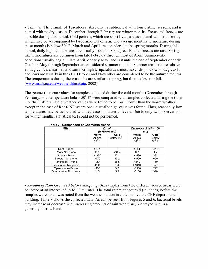
• Climate. The climate of Tuscaloosa, Alabama, is subtropical with four distinct seasons, and is humid with no dry season. December through February are winter months. Frosts and freezes are possible during this period. Cold periods, which are short lived, are associated with cold fronts, which may be accompanied by large amounts of rain. The average monthly temperature during these months is below 500 F. March and April are considered to be spring months. During this period, daily high temperatures are usually less than 80 degrees F., and freezes are rare. Spring-like temperatures are common from late February through most of April. Summer-like conditions usually begin in late April, or early May, and last until the end of September or early October. May through September are considered summer months. Summer temperatures above 90 degree F. are normal, and summer high temperatures almost never drop below 80 degrees F, and lows are usually in the 60s. October and November are considered to be the autumn months. The temperatures during these months are similar to spring, but there is less rainfall. (www.math.ua.edu/weather.htm#data, 2002).

The geometric mean values for samples collected during the cold months (December through February, with temperature below 500 F) were compared with samples collected during the other months (Table 7). Cold weather values were found to be much lower than the warm weather, except in the case of Roof- NP where one unusually high value was found. Thus, seasonally low temperatures may be associated with decreases in bacterial levels. Due to only two observations for winter months, statistical test could not be performed.

Table 7. Comparison of Geometric Means Site E. coli

(MPN/100 mL) Enterococci (MPN/100

mL) Warm Above 500 F

Cold Below 500 F

Warm Above 500 F

Cold Below 500 F

Roof - Prone Roof - Not prone

>574 1 10.5 >34.7

>684 22.5 8.7 1.2

Streets- Prone Streets- Not prone

>1330 12.1 >470 83.2

>4530 332 >1500 650

Parking lot - Prone Parking lot- Not prone

129 28.5 45.8 1.4

>640 160 >1010 85.8

Open space- Prone Open space- Not prone

>130 3.2 110 5.9

>3500 292 >6100 310

• Amount of Rain Occurred before Sampling. Six samples from two different source areas were collected at an interval of 15 to 30 minutes. The total rain that occurred (in inches) before the samples were taken was noted from the weather station installed above the CEE departmental building. Table 8 shows the collected data. As can be seen from Figures 5 and 6, bacterial levels may increase or decrease with increasing amounts of rain with time, but stayed within a generally narrow band.

Table 8. Effect of Total Rain and Rain Intensity on Bacterial Levels Time of

Sampling Total Rain Occurred

5 Minute Rain Rate

Street - NP Parking Lot - NP

(inches) (in/hr) E. coli MPN/100 mL

Enterococci MPN/100 mL

E. coli MPN/100 mL

Enterococci MPN/100 mL

9 A.M 0.29 0.29 1553.1 130 16 3654 9.15 A.M 0.35 0.46 547.5 107 18.7 3255 9.30 A.M 0.4 0.06 1046.2 738 10.9 3255 9.45 A.M 0.44 0.17 517.2 364 17.3 4352 10 A.M 0.47 0.09 920.8 712 7.4 1014

10.30 A.M 0.48 0.04 980.4 1106 16 1376

Effect of total rain (in) occured before sampling on bacterial levels Street- NP

1

10

100

1000

10000

0.25 0.3 0.35 0.4 0.45 0.5

Total rain (in)

E. coli

Enterococci

Figure 5. Effect of Total Rain on Bacterial Levels (Street- NP)

Effect of total rain (in) occured before sampling on bacterial levels Parking lot - NP

1

10

100

1000

10000

0.25 0.3 0.35 0.4 0.45 0.5

Total rain (in)

E. coli

Enterococci

Figure 6. Effect of Total Rain on Bacterial Levels (Parking Lot- NP)

Regression analyses and associated ANOVA tests were conducted to determine the significance of the slope term in the relationship between total rain depth and bacterial levels. In all cases, no significant relationship likely exists between total rain depth and bacterial levels.

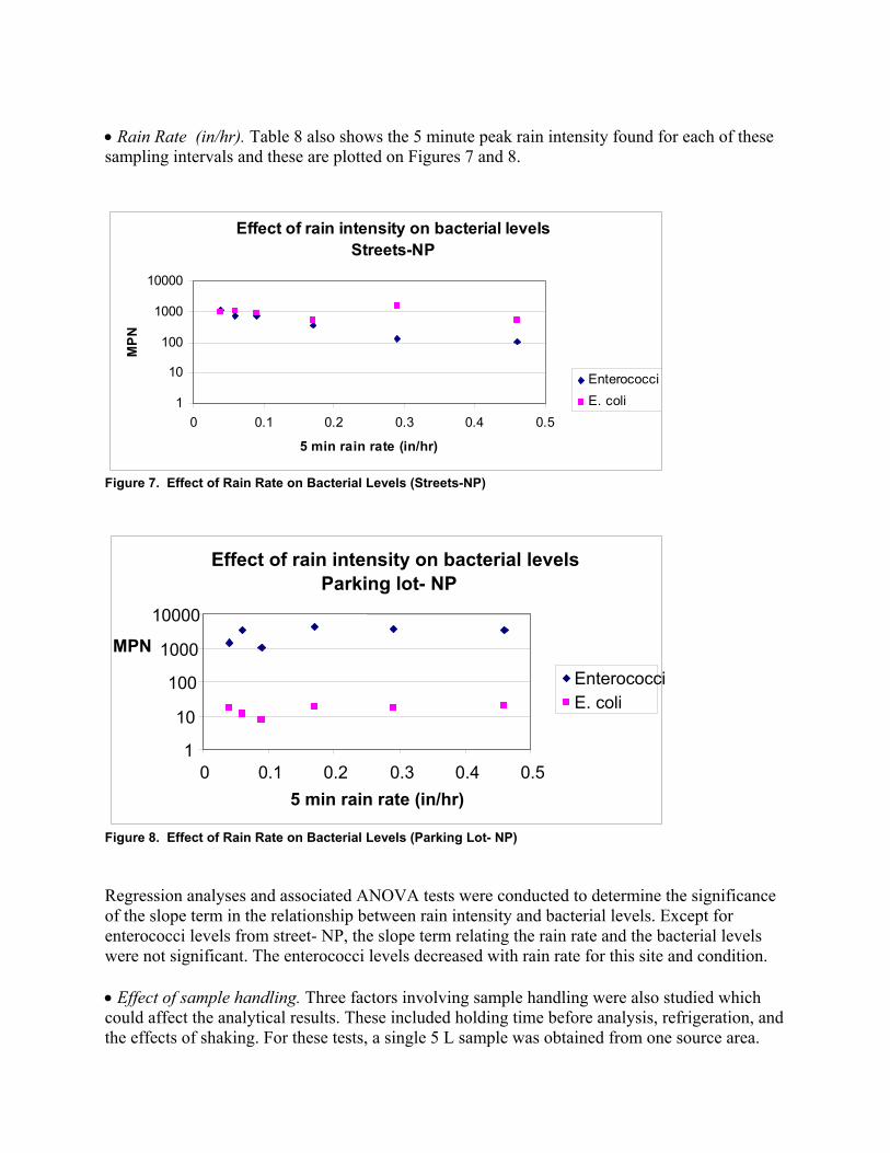
• Rain Rate (in/hr). Table 8 also shows the 5 minute peak rain intensity found for each of these sampling intervals and these are plotted on Figures 7 and 8.

Effect of rain intensity on bacterial levels Streets-NP

1

10

100

1000

10000

0 0.1 0.2 0.3 0.4 0.5

5 min rain rate (in/hr)

MP

N

Enterococci E. coli

Figure 7. Effect of Rain Rate on Bacterial Levels (Streets-NP)

Effect of rain intensity on bacterial levels Parking lot- NP

1

10

100

1000

10000

0 0.1 0.2 0.3 0.4 0.5 5 min rain rate (in/hr)

MPN

Enterococci E. coli

Figure 8. Effect of Rain Rate on Bacterial Levels (Parking Lot- NP)

Regression analyses and associated ANOVA tests were conducted to determine the significance of the slope term in the relationship between rain intensity and bacterial levels. Except for enterococci levels from street- NP, the slope term relating the rain rate and the bacterial levels were not significant. The enterococci levels decreased with rain rate for this site and condition.

• Effect of sample handling. Three factors involving sample handling were also studied which could affect the analytical results. These included holding time before analysis, refrigeration, and the effects of shaking. For these tests, a single 5 L sample was obtained from one source area.

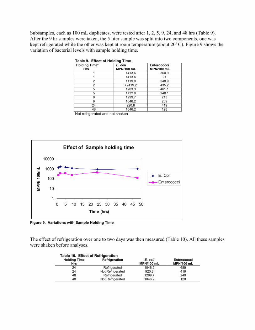
Subsamples, each as 100 mL duplicates, were tested after 1, 2, 5, 9, 24, and 48 hrs (Table 9). After the 9 hr samples were taken, the 5 liter sample was split into two components, one was kept refrigerated while the other was kept at room temperature (about 20o C). Figure 9 shows the variation of bacterial levels with sample holding time.

Table 9. Effect of Holding Time Holding Time*

Hrs E. coli MPN/100 mL

Enterococci MPN/100 mL

1 1413.6 360.9 1 1413.6 91 2 1119.9 248.9 2 >2419.2 435.2 5 1203.3 461.1 5 1732.9 248.1 9 1299.7 213 9 1046.2 269

24 920.8 419 48 1046.2 128

Not refrigerated and not shaken

Effect of Sample holding time

1

10

100

1000

10000

0 5 10 15 20 25 30 35 40 45 50

Time (hrs)

MPN

/ 100

mL

E. Coli Enterococci

Figure 9. Variations with Sample Holding Time

The effect of refrigeration over one to two days was then measured (Table 10). All these samples were shaken before analyses.

Table 10. Effect of RefrigerationHolding Time

Hrs Refrigeration E. coli

MPN/100 mL Enterococci MPN/100 mL

24 24

Refrigerated Not Refrigerated

1046.2 920.8

689 419

48 Refrigerated 1299.7 240 48 Not Refrigerated 1046.2 128

The effect of shaking was measured by first taking a 100 mL sample from the unshaken larger sample container, and later shaking the larger sample bottle and testing another 100 mL sample (Table 11).

Table 11. Effect of ShakingHolding Time

Hrs Shaking E. coli

MPN/100 mL Enterococci MPN/100 mL

24 Shaken 920.8 419 24 Not shaken 920.8 298.7 48 Shaken 1046.2 128 48 Not shaken 488.4 30

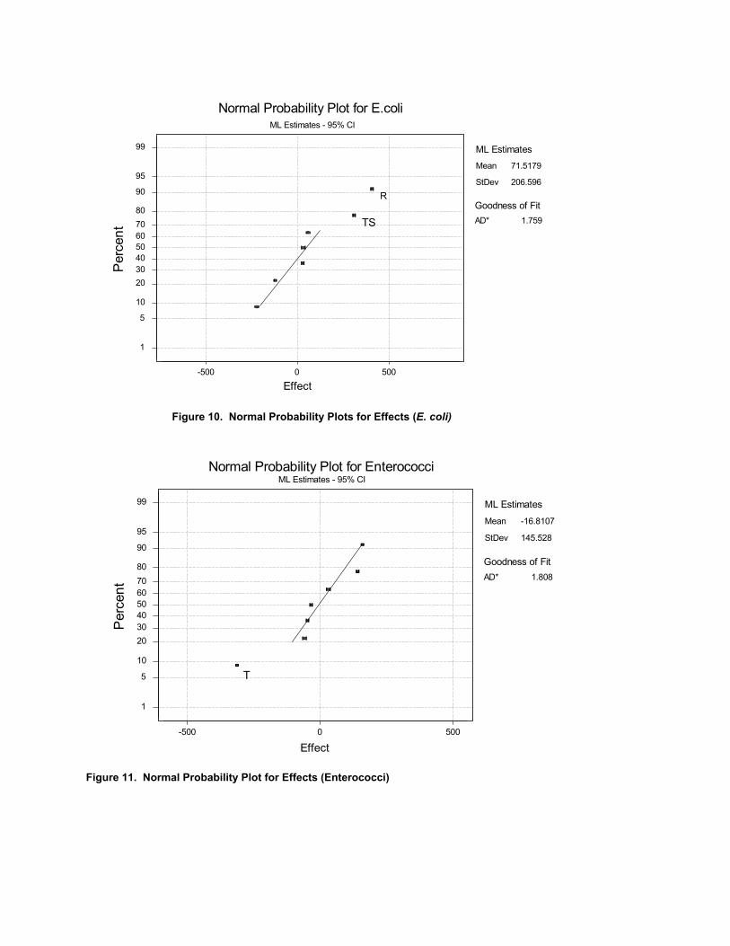
A 23 factorial evaluation was conducted to identify the main effects and effects of interactions between these handling factors. Table 12 shows the factorial design. The calculated main effects and interaction effects are shown in Table 13 and the normal probability plot of the effects are shown on Figures 10 and 11, indicating the significant factors and interactions.

Table 12. Factorial Design Experiment no. Time

(T) - 24 hr

Refrigeration _ Not + Yes

(R) Shaking (S)

_ No

E. coli MPN/100 mL

Enterococci MPN/100 mL

+ 48hr + Yes 1 - - - 920.8 298.7 2 + - - 488.4 30 3 - + - 1553.1 413 4 + + - 1119.9 173 5 - - + 920.8 419 6 + - + 1046.2 128 7 - + + 1046.2 689 8 + + + 1299.7 240

Average 1049.4 298.8

Table 13. Main Effects and Interaction Effects

Indicator Main Effects Interaction Effects

Time Shaking (T) Refrigeration( R ) (S)

E. coli -121.6 410.6 57.6 TS

311.1 TR RS

31.8 -221.2 TRS 32.2

Enterococci -312.1 159.8 140.3 -57.8 -32.3 31.1 -46.6

Interpretations are needed for R and TS for E. coli and T only for enterococci, as can be seen from the probability plots of effects (Figures 10 and 11). Based on these effects, the calculated values were found using the equations:

Value = Avg. ± (effects / 2)( factor) E.Coli = 1049 ± (411/ 2)(R) ± (311/ 2)(TS)Enterococci = 298.8 ± (−312.1/ 2)(T )

Tables 14 and 15 shows the calculated and observed values for various conditions.

Normal Probability Plot for E.coli ML Estimates - 95% CI

1

5

10

20 30 40 50 60 70 80

90

95

99

Per

cent

AD* 1.759

Goodness of Fit

Mean

StDev

71.5179

206.596

ML Estimates

R

TS

-500 0 500

Effect

Figure 10. Normal Probability Plots for Effects (E. coli)

Normal Probability Plot for Enterococci ML Estimates - 95% CI

1

5

10

20 30 40 50 60 70 80

90

95

99

Per

cent

AD* 1.808

Goodness of Fit

Mean

StDev

-16.8107

145.528

ML Estimates

T

-500 0 500

Effect

Figure 11. Normal Probability Plot for Effects (Enterococci)

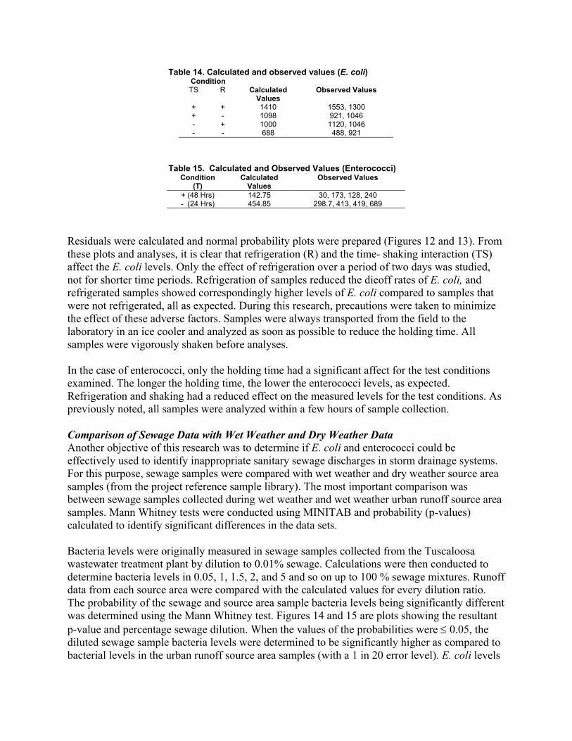
Table 14. Calculated and observed values (E. coli)Condition TS R Calculated Observed Values

Values + + 1410 1553, 1300 + - 1098 921, 1046 - + 1000 1120, 1046 - - 688 488, 921

Table 15. Calculated and Observed Values (Enterococci) Condition Calculated Observed Values

(T) Values + (48 Hrs) 142.75 30, 173, 128, 240 - (24 Hrs) 454.85 298.7, 413, 419, 689

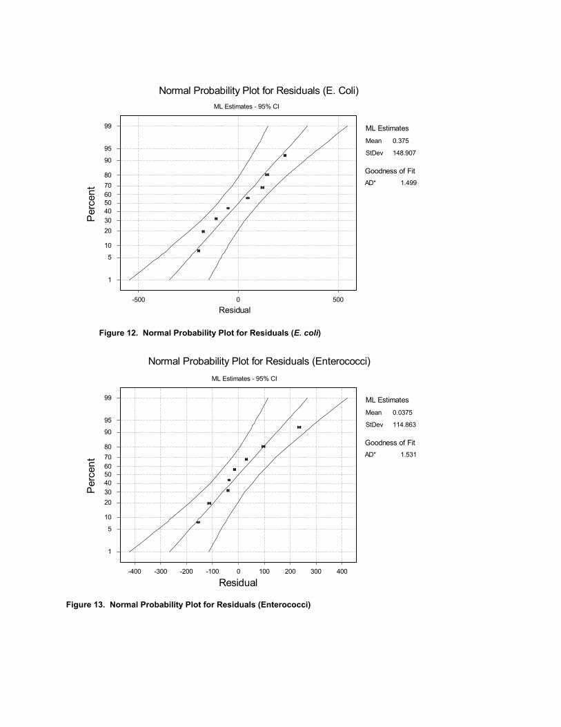
Residuals were calculated and normal probability plots were prepared (Figures 12 and 13). From these plots and analyses, it is clear that refrigeration (R) and the time- shaking interaction (TS) affect the E. coli levels. Only the effect of refrigeration over a period of two days was studied, not for shorter time periods. Refrigeration of samples reduced the dieoff rates of E. coli, and refrigerated samples showed correspondingly higher levels of E. coli compared to samples that were not refrigerated, all as expected. During this research, precautions were taken to minimize the effect of these adverse factors. Samples were always transported from the field to the laboratory in an ice cooler and analyzed as soon as possible to reduce the holding time. All samples were vigorously shaken before analyses.

In the case of enterococci, only the holding time had a significant affect for the test conditions examined. The longer the holding time, the lower the enterococci levels, as expected. Refrigeration and shaking had a reduced effect on the measured levels for the test conditions. As previously noted, all samples were analyzed within a few hours of sample collection.

Comparison of Sewage Data with Wet Weather and Dry Weather Data Another objective of this research was to determine if E. coli and enterococci could be effectively used to identify inappropriate sanitary sewage discharges in storm drainage systems. For this purpose, sewage samples were compared with wet weather and dry weather source area samples (from the project reference sample library). The most important comparison was between sewage samples collected during wet weather and wet weather urban runoff source area samples. Mann Whitney tests were conducted using MINITAB and probability (p-values) calculated to identify significant differences in the data sets.

Bacteria levels were originally measured in sewage samples collected from the Tuscaloosa wastewater treatment plant by dilution to 0.01% sewage. Calculations were then conducted to determine bacteria levels in 0.05, 1, 1.5, 2, and 5 and so on up to 100 % sewage mixtures. Runoff data from each source area were compared with the calculated values for every dilution ratio. The probability of the sewage and source area sample bacteria levels being significantly different was determined using the Mann Whitney test. Figures 14 and 15 are plots showing the resultant p-value and percentage sewage dilution. When the values of the probabilities were ≤ 0.05, the diluted sewage sample bacteria levels were determined to be significantly higher as compared to bacterial levels in the urban runoff source area samples (with a 1 in 20 error level). E. coli levels

Normal Probability Plot for Residuals (E. Coli) ML Estimates - 95% CI

99

95

90

80 70 60 50 40 30 20

10

5

1

Per

cent

1.499AD*

Goodness of Fit

Mean

StDev

0.375

148.907

ML Estimates

-500 0 500

Residual

Figure 12. Normal Probability Plot for Residuals (E. coli)

Normal Probability Plot for Residuals (Enterococci) ML Estimates - 95% CI

99

95

90

80 70 60 50 40 30 20

10

5

1

Per

cent

1.531AD*

Goodness of Fit

Mean

StDev

0.0375

114.863

ML Estimates

-400 -300 -200 -100 0 100 200 300 400

Residual

Figure 13. Normal Probability Plot for Residuals (Enterococci)

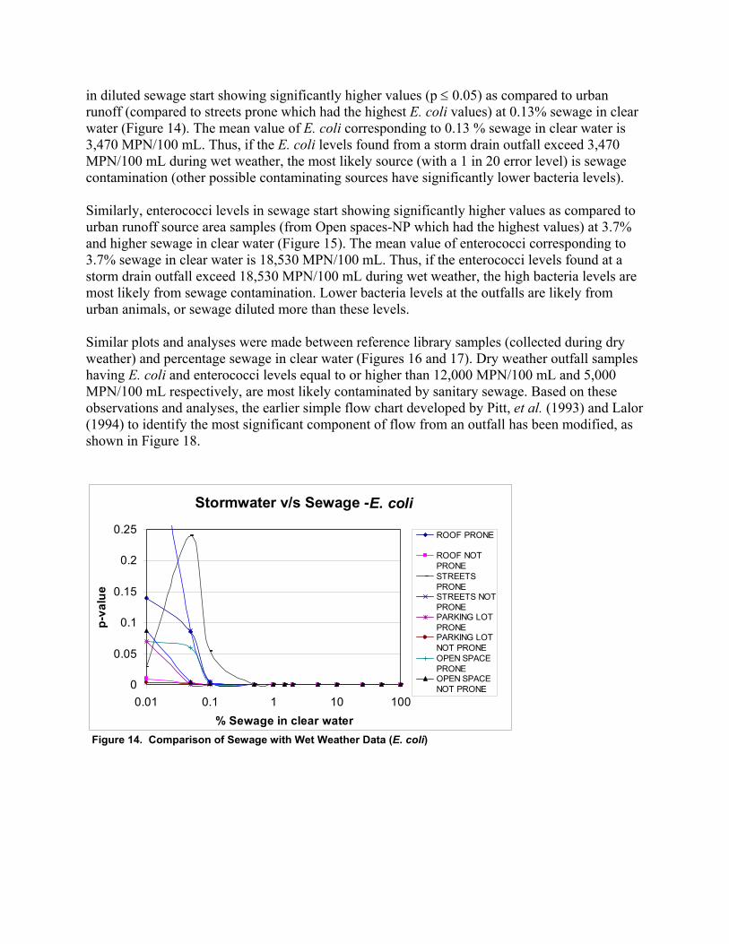
in diluted sewage start showing significantly higher values (p ≤ 0.05) as compared to urban runoff (compared to streets prone which had the highest E. coli values) at 0.13% sewage in clear water (Figure 14). The mean value of E. coli corresponding to 0.13 % sewage in clear water is 3,470 MPN/100 mL. Thus, if the E. coli levels found from a storm drain outfall exceed 3,470 MPN/100 mL during wet weather, the most likely source (with a 1 in 20 error level) is sewage contamination (other possible contaminating sources have significantly lower bacteria levels).

Similarly, enterococci levels in sewage start showing significantly higher values as compared to urban runoff source area samples (from Open spaces-NP which had the highest values) at 3.7% and higher sewage in clear water (Figure 15). The mean value of enterococci corresponding to 3.7% sewage in clear water is 18,530 MPN/100 mL. Thus, if the enterococci levels found at a storm drain outfall exceed 18,530 MPN/100 mL during wet weather, the high bacteria levels are most likely from sewage contamination. Lower bacteria levels at the outfalls are likely from urban animals, or sewage diluted more than these levels.

Similar plots and analyses were made between reference library samples (collected during dry weather) and percentage sewage in clear water (Figures 16 and 17). Dry weather outfall samples having E. coli and enterococci levels equal to or higher than 12,000 MPN/100 mL and 5,000 MPN/100 mL respectively, are most likely contaminated by sanitary sewage. Based on these observations and analyses, the earlier simple flow chart developed by Pitt, et al. (1993) and Lalor (1994) to identify the most significant component of flow from an outfall has been modified, as shown in Figure 18.

Stormwater v/s Sewage -E. coli

0

0.05

0.1

0.15

0.2

0.25

0.01 0.1 1 10 100 % Sewage in clear water

p-va

lue

ROOF PRONE

ROOF NOT PRONE STREETS PRONE STREETS NOT PRONE PARKING LOT PRONE PARKING LOT NOT PRONE OPEN SPACE PRONE OPEN SPACE NOT PRONE

Figure 14. Comparison of Sewage with Wet Weather Data (E. coli)

Stormwater v/s Sewage - Enterococci

0

0.1

0.2

0.3

0.4

0.5

0.6

0.01 0.1 1 10 100

% Sewage in clear water

p-va

lue

ROOF PRONE

ROOF NOT PRONE STREETS PRONE

STREETS NOT PRONE PARKING LOT PRONE PARKING LOT NOT PRONE OPEN SPACE PRONE OPEN SPACE NOT PRONE

Figure 15. Comparison of Sewage with Wet Weather Data (Enterococci)

Library samples v/s sewage-E. coli

0

0.05

0.1

0.15

0.2

0.25

0.3

0.35

0.4

0.45

0.01 0.1 1 10 100 % sewage in clear water

p- v

alue

Tap water Spring water Irrigation Laundry Car wash industrial

Figure 16. Comparison of Sewage with Dry Weather Data (E. coli)

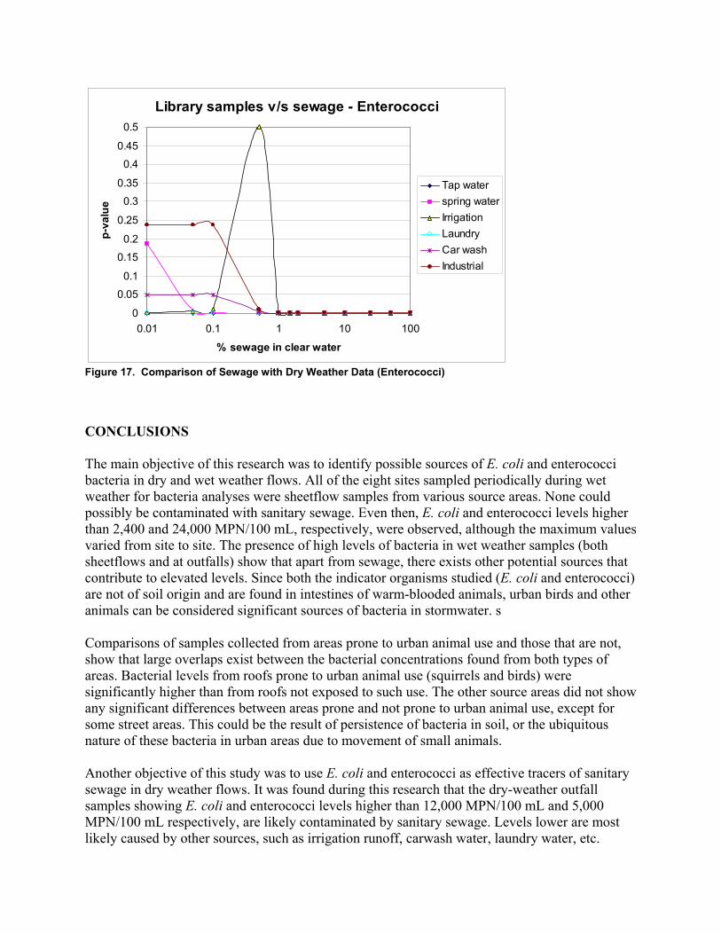
Library samples v/s sewage - Enterococci

0

0.05

0.1

0.15

0.2

0.25

0.3

0.35

0.4

0.45

0.5

0.01 0.1 1 10 100

% sewage in clear water

p-va

lue

Tap water spring water Irrigation Laundry Car wash Industrial

Figure 17. Comparison of Sewage with Dry Weather Data (Enterococci)

CONCLUSIONS

The main objective of this research was to identify possible sources of E. coli and enterococci bacteria in dry and wet weather flows. All of the eight sites sampled periodically during wet weather for bacteria analyses were sheetflow samples from various source areas. None could possibly be contaminated with sanitary sewage. Even then, E. coli and enterococci levels higher than 2,400 and 24,000 MPN/100 mL, respectively, were observed, although the maximum values varied from site to site. The presence of high levels of bacteria in wet weather samples (both sheetflows and at outfalls) show that apart from sewage, there exists other potential sources that contribute to elevated levels. Since both the indicator organisms studied (E. coli and enterococci) are not of soil origin and are found in intestines of warm-blooded animals, urban birds and other animals can be considered significant sources of bacteria in stormwater. s

Comparisons of samples collected from areas prone to urban animal use and those that are not, show that large overlaps exist between the bacterial concentrations found from both types of areas. Bacterial levels from roofs prone to urban animal use (squirrels and birds) were significantly higher than from roofs not exposed to such use. The other source areas did not show any significant differences between areas prone and not prone to urban animal use, except for some street areas. This could be the result of persistence of bacteria in soil, or the ubiquitous nature of these bacteria in urban areas due to movement of small animals.

Another objective of this study was to use E. coli and enterococci as effective tracers of sanitary sewage in dry weather flows. It was found during this research that the dry-weather outfall samples showing E. coli and enterococci levels higher than 12,000 MPN/100 mL and 5,000 MPN/100 mL respectively, are likely contaminated by sanitary sewage. Levels lower are most likely caused by other sources, such as irrigation runoff, carwash water, laundry water, etc.

Land Use Flow Check Parameter Check Result

Start

Land use

YesResidential

Ammonia/ potassium ratio >1.0

No

Check for dry-weather flow

Yes

Yes

Yes

Flow?

NoIndustrial or E.coli >12,000

MPN/100mL or Enterococci

>5,000 MPN/100mL

Detergent >0.25 mg/L

or Boron >0.35 mg/L

NoNo commercial

Yesindustrial/

No No

Fluorescence >25 mg/L

Fluoride >0.25 mg/L

No

Recheck per permitrequirements

Fluoride >0.6 mg/L

Yes

Possible sanitary wastewater

contamination

Possible washwater

contamination

Yes Likely irrigation water source

Likely natural water source

Likely tap water source

Use industrial/ commercial checklist

(Pitt 1993a)

Figure 18. Modified Flow Chart to Identify Most Significant Flow Component

REFERENCES

EPA. January 1986. Ambient Water Quality Criteria for Bacteria. Office of Water Regulations and Standards, Criteria and Standards Division. EPA 440/5-84-002.

Lalor, M. 1994. Assessment of non-stormwater discharges to storm drainage systems in residential and commercial land use areas. Ph.D. thesis. Department of environmental and water resources engineering. Vanderbilt University. Nashville, TN.

Pitt, R., M. Lalor, R. Field, D.D. Adrian, and D. Barbe’. January 1993. A User’s Guide for the Assessment of Non-Stormwater Discharges into Separate Storm Drainage Systems. Jointly published by the Center of Environmental Research Information, US EPA, and the Urban Waste Management & Research Center (UWM&RC). EPA/600/R-92/238. PB93-131472. Cincinnati, Ohio.

Shergill, S. Quantification of Escherichia Coli and Enterococci Levels in Wet Weather and Dry Weather Flows. Masters thesis, Department of Civil and Environmental Engineering, the University of Alabama. Tuscaloosa, AL. May 2004.

Standard Methods for the Examination of Water and Wastewater - 20th edition. 1998. Washington D.C. Edited by Lenore S. Clesceri, Arnold E. Greenberg and Andrew D. Eaton. Published by American public health association, American water works association and Water environment federation.