Embed Size (px)
Citation preview

Quantification of the Performance of Iterative and Non-Iterative
Computational Methods of Locating Partial Discharges Using RF
Measurement Techniques
Othmane El Mountassir 1*
, Brian G Stewart 2, Alistair J Reid
3 and Scott G McMeekin
4
1 Offshore Renewable Energy Catapult, 121 George Street, Glasgow G1 1RD, UK
2 Department of Electronic and Electrical Engineering, University of Strathclyde, 204 George Street, Glasgow G1 1XW, UK
3 School of Engineering, Cardiff University, The Parade, Cardiff CF24 3AA, UK
4 Institute for Sustainable Engineering & Technology, Glasgow Caledonian University, 70 Cowcaddens Road, Glasgow G4 0BA,
UK
Abstract
Partial discharge (PD) is an electrical discharge phenomenon that occurs when the 1
insulation material of high voltage equipment is subjected to high electric field stress. 2
Its occurrence can be an indication of incipient failure within power equipment such as 3
power transformers, underground transmission cable or switchgear. Radio frequency 4
measurement methods can be used to detect and locate discharge sources by measuring 5
the propagated electromagnetic wave arising as a result of ionic charge acceleration. An 6
array of at least four receiving antennas may be employed to detect any radiated 7
discharge signals, then the three dimensional position of the discharge source can be 8
calculated using different algorithms. These algorithms fall into two categories; iterative 9
or non-iterative. 10
This paper evaluates, through simulation, the location performance of an iterative 11
method (the standard least squares method) and a non-iterative method (the Bancroft 12
algorithm). Simulations were carried out using (i) a “Y” shaped antenna array and (ii) a 13
square shaped antenna array, each consisting of a four-antennas. The results show that 14
PD location accuracy is influenced by the algorithm’s error bound, the number of 15
iterations and the initial values for the iterative algorithms, as well as the antenna 16
arrangement for both the non-iterative and iterative algorithms. Furthermore, this 17
*ManuscriptClick here to view linked References

research proposes a novel approach for selecting adequate error bounds and number of 18
iterations using results of the non-iterative method, thus solving some of the iterative 19
method dependencies. 20
Keywords: Partial discharges; Iterative algorithms; Non-Iterative algorithms; Radio 21
Frequency; Fault location; Time difference of arrival. 22

1 Introduction 23
Radio frequency (RF) measurement technique using receiving antennas can be used to 24
detect the radiated energy from PD sources or any other electrical discharge activities, 25
subsequently facilitating the discharge source triangulation. Using a receiving antenna 26
array, which may be arranged in various forms, the time differences of arrival (TDOA) 27
between received signals on each of the respective antennas allows the 3 dimensional 28
position of the electrical discharge source to be deduced by processing of the TDOA 29
values through iterative or non-iterative location algorithms. The location of partial 30
discharges using emitted RF techniques in HV equipment has been widely investigated 31
[1-5]. Research in this area has been carried out on cables [6-9], gas and air insulated 32
switchgears [10-14] and transformers [15-17]. PD location in cables, and to a degree in 33
gas-insulated substation (GIS), is a two-dimensional problem, while internal localisation 34
within power transformers and localisation in three dimensions in wide-area HV 35
substations requires robust computation algorithms [1]. 36
There are two types of computational algorithm which can be used to locate partial 37
discharges in three dimensions; (i) iterative methods and (ii) non-iterative methods. In 38
this study, a non-iterative method was selected due to the large success of these methods 39
in Global Positioning System (GPS) applications such as navigation and location 40
systems. The choice of an iterative method was mainly due their efficiency in solving 41
nonlinear problems involving large number of variables. 42
The iterative methods give an approximate solution to nonlinear equations based on a 43
number of iterations and starting with an initial value, which is improved at each 44
iteration by an error bound until a converged solution is found or until a maximum 45
number of iterations is reached. Taylor expansion and Newton-Raphson techniques are 46
common iterative methods that can be used to solve the equations of nonlinear systems. 47

These methods have been used in different studies to locate PD [1, 18-19]. The study in 48
[18] highlighted that the performance of the Taylor expansion method depends on the 49
accuracy of the initial values and the number of sensors, whereas the study by [1] 50
showed that the Newton-Raphson method successfully locates PD and that the location 51
accuracy depends on the arrangement of antennas. Study [19] also used the Newton-52
Raphson method to locate PD and found that in some cases the algorithm did not 53
provide a converged solution. It indicated that a solution called the “grid search 54
method” which consists of using a range of values within a grid as initial values to 55
determine a converged solution helped improve accuracy. Despite the fact that these 56
studies highlighted the success of these iterative methods to locate discharges activities 57
within a reasonable margin of error, a limited number of published studies have 58
attempted to evaluate fully the performance of non-iterative and iterative methods in 59
their ability to locate accurately the position of electrical discharge sources. 60
In order to evaluate the performance of iterative and non-iterative algorithms, the 61
present study investigates through simulation the location performance of a well-62
established iterative method; the standard least squares (SLS) method, and a non-63
iterative method; the Bancroft algorithm [22]. Two antenna array configurations (Y and 64
square shape), both consisting of 4 antenna positions were chosen for the investigations 65
reported herein evaluating the performance of the respective location algorithms. The 66
square and ‘Y’ array configurations are commonly used and were selected since they 67
have been used in previous studies [1, 4] to investigate electromagnetic (EM) wave 68
propagation PD sources. 69
The paper is structured as follows: The mathematical formulation of the SLS and 70
Bancroft location algorithms are presented in Section II; Section III presents the 71
methodologies used in the present study; Section IV presents the results of PD location 72

studies using the SLS and Bancroft algorithms respectively (in each case two different 73
antenna arrangements were investigated). For simplification, the simulated PD location 74
data points refer to any electrical discharge source emitting EM wave radiation; Section 75
V compares the characteristics of both the iterative and non-iterative algorithms used; 76
Section VI proposes a new approach to select adequate error bounds and number of 77
iterations using results of the non-iterative methods; Section VII summarises the 78
findings of the study. 79
2 Formulation of the SLS and Bancroft Algorithms 80
A minimum of four spatially separated antennas may be used to triangulate the location 81
of a PD event in 3 dimensions using RF methods (Figure 1). Knowing the grid 82
coordinates of each antenna in the array then allows the propagation time from the PD 83
source to the respective antennas to be calculated using the basic formula D = v.t, 84
Where D is distance, v is propagation velocity and t is propagation time. This technique, 85
commonly referred to as ‘triangulation’, is described by Equation (1): 86
2iteV2
izz2
iyy2
ixx (1) 87
Figure 1: Basic configuration of a typical RF PD location setup. 88
Where (xi, yi, zi) are the coordinates of the ith
antenna in Cartesian space, (x, y, z) 89
represent the true coordinates of the PD event, ve is the speed of light (3 x10⁸ m/s) and ti 90

represents the ‘time-of-flight’ of the propagating PD signal from its source to the ith
91
antenna. It should be noted that since the study is a simulation based investigation, the 92
speed of light was considered to be in a vacuum and that this value changes depending 93
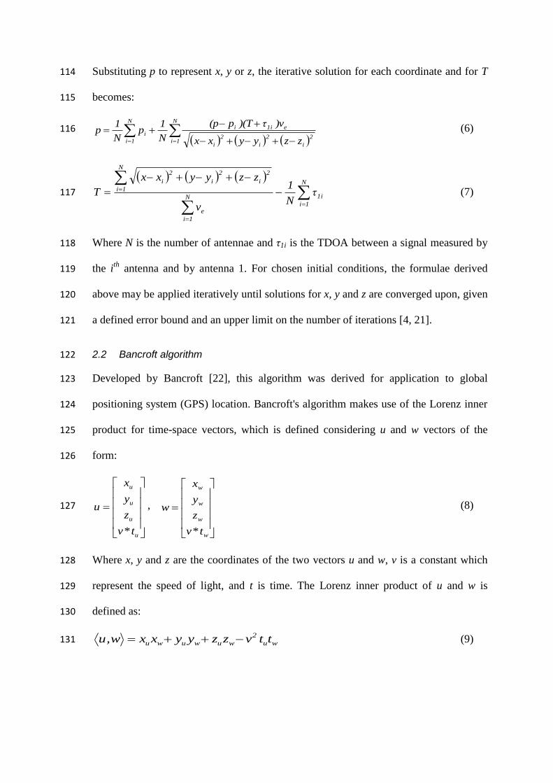
on the insulating material. 94
Let the time-of-flight from the PD source to antenna A1 be T and the time-difference-of-95
arrival between antennas A1 and An (n = 2, 3, 4) be 1n. Equation (1) now expands into 96
the following four formulae [20]: 97
2Tev2
1zz2
1yy2
1xx 98
2)12τ(Tev
2
2zz2
2yy2
2xx 99
2)13τ(Tev
2
3zz2
3yy2
3xx 100
2)14τ(Tev
2
4zz2
4yy2
4xx (2) 101
2.1 Standard Least Squares (SLS) algorithm 102
Using on the non-linear equations in (2), the position of a PD source (x, y, z) can be 103
computed using the least squares method given in Equation (3). 104
N
1i
2
i XYXS (3) 105
In least squares, the standard definition of Yi(X) is given in Equation (4). Based on the 106
definition of Yi(X), the least squares method minimises the sum of the square of the 107
residuals. 108
)T(*vzzyyxx)X(Y i1e
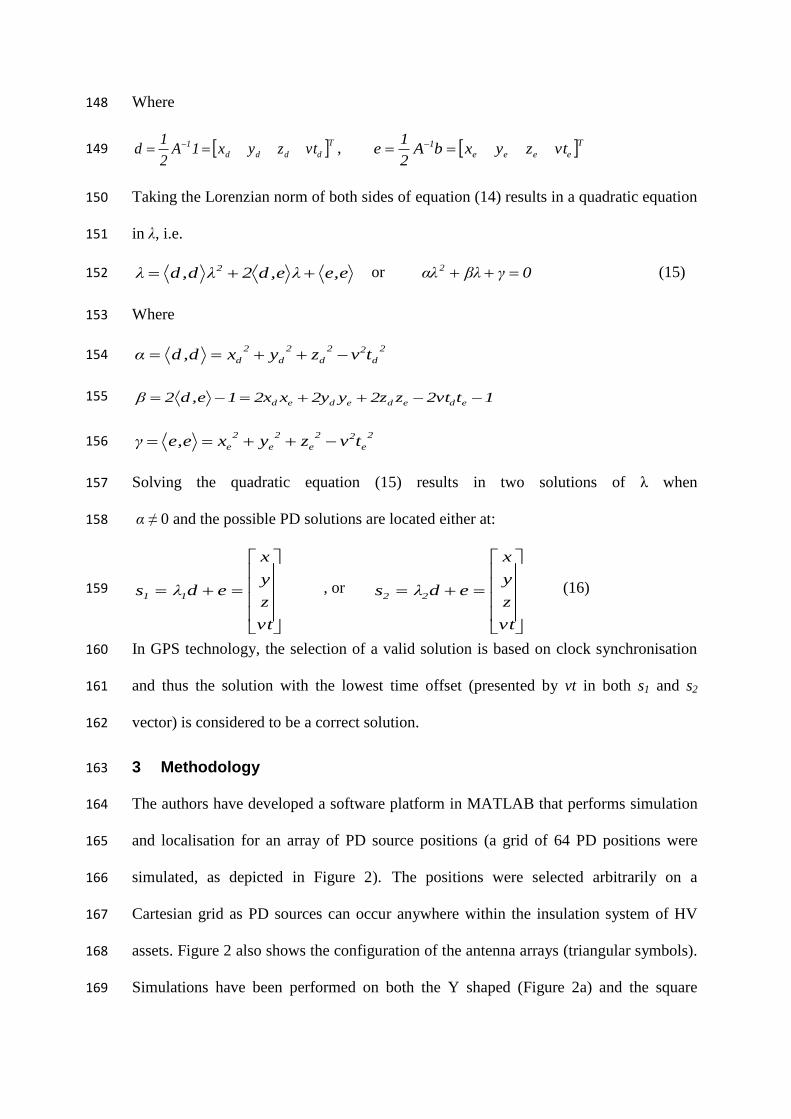
2
i
2
i
2
ii (4) 109
Since the aim is to compute the values of x, y and z which minimise S(X), the partial 110
derivative of S(X) with respect to x, y and z is calculated with the equation set equal to 0 111
as shown in Equation (5): 112
0x
S
, 0
y
S
, 0z
S
and 0
T
S
. (5) 113
Substituting p to represent x, y or z, the iterative solution for each coordinate and for T 114
becomes: 115
N
1i2
i
2
i
2
i
ei1iN
1i
i
zzyyxx
v)τ)(Tp(p
N
1p
N
1p (6) 116
N
1i
i1N
1i
e
N
1i
2
i
2
i
2
i
τN
1
v
zzyyxx
T (7) 117
Where N is the number of antennae and τ1i is the TDOA between a signal measured by 118
the ith
antenna and by antenna 1. For chosen initial conditions, the formulae derived 119
above may be applied iteratively until solutions for x, y and z are converged upon, given 120
a defined error bound and an upper limit on the number of iterations [4, 21]. 121
2.2 Bancroft algorithm 122
Developed by Bancroft [22], this algorithm was derived for application to global 123
positioning system (GPS) location. Bancroft's algorithm makes use of the Lorenz inner 124
product for time-space vectors, which is defined considering u and w vectors of the 125
form: 126
u
u
u
u
tv*
z
y
x
u ,
w
w
w
w
tv*
z
y
x
w (8) 127
Where x, y and z are the coordinates of the two vectors u and w, v is a constant which 128
represent the speed of light, and t is time. The Lorenz inner product of u and w is 129
defined as: 130
wu
2
wuwuwu ttvzzyyxxw,u (9) 131

Assuming there are four antennas located at (xi, yi, zi), with the associated time of arrival 132
(TOA) as ti, where i = 1, 2, 3, 4 and the PD source is located at (x, y, z) and has a time 133
of emission (TOE) t. This can presented as: 134
i
i
i
i
i
tv*
z
y
x
s ,
tv*
z
y
x
s (10) 135
Each TOA measurement may be expressed as: 136
2
i
22
i
2
i
2
i )t(t*vzzyyxx (11) 137
Which is equivalent to: 138
i222
i
2
i
2
i
22222
i
2
iii tvzyxtvzyxttvzzyyxx2 (12) 139
or, in vector-matrix form: 140
bλ12As (13) 141
Where 142
tv*
z
y
x
s , are the coordinates of interest 143
4444
3333
2222
1111
vtzyx
vtzyx
vtzyx
vtzyx
A , 22222 tvzyxs,sλ and
1
1
1
1
1 144
2
4
22
4
2
4
2
4
2
3
22
3
2
3
2
3
2
2
22
2
2
2
2
2
2
1
22
1
2
1
2
1
44
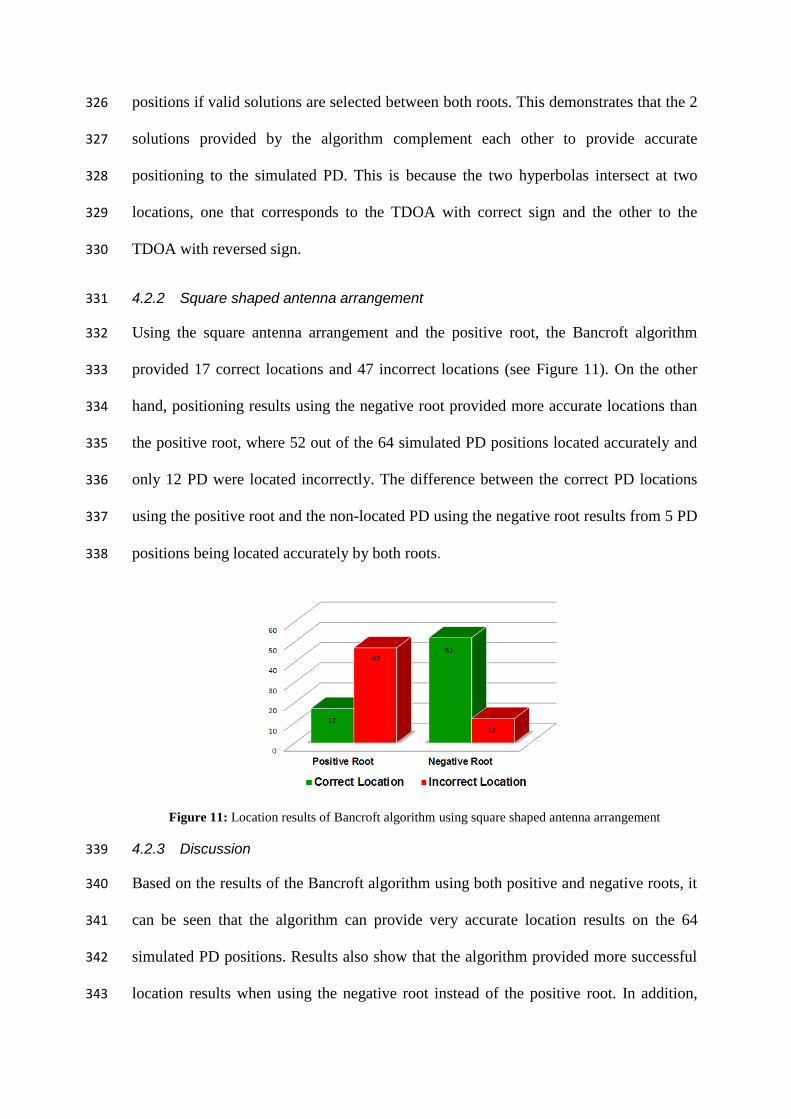
33
22
11
tvzyx
tvzyx
tvzyx
tvzyx
s,s
s,s
s,s
s,s
b 145
Based on equation (13), which relates s to its Lorenzian norm λ, this can be rewritten as: 146
bA2
11λA
2
1s 11 or eλds (14) 147
Where 148
Tdddd
1 vtzyx1A2
1d , Teeee
1 vtzyxbA2
1e 149
Taking the Lorenzian norm of both sides of equation (14) results in a quadratic equation 150
in λ, i.e. 151
e,eλe,d2λd,dλ 2 or 0γβλαλ 2 (15) 152
Where 153
2
d
22
d
2
d
2
d tvzyxd,dα 154
1t2vtz2zy2yx2x1e,d2β edededed 155
2
e
22
e
2
e
2
e tvzyxe,eγ 156
Solving the quadratic equation (15) results in two solutions of λ when 157
α ≠ 0 and the possible PD solutions are located either at: 158
vt
z
y
x
edλs 11 , or
vt
z
y
x
edλs 22 (16) 159
In GPS technology, the selection of a valid solution is based on clock synchronisation 160
and thus the solution with the lowest time offset (presented by vt in both s1 and s2 161
vector) is considered to be a correct solution. 162
3 Methodology 163
The authors have developed a software platform in MATLAB that performs simulation 164
and localisation for an array of PD source positions (a grid of 64 PD positions were 165
simulated, as depicted in Figure 2). The positions were selected arbitrarily on a 166
Cartesian grid as PD sources can occur anywhere within the insulation system of HV 167
assets. Figure 2 also shows the configuration of the antenna arrays (triangular symbols). 168
Simulations have been performed on both the Y shaped (Figure 2a) and the square 169

shaped array (Figure 2b). Table 1 presents the grid coordinates of each antenna. These 170
antenna arrangement arrays were considered in a way to enable an easy setting of these 171
equipment when measurements are carried out in a real site environment, although 172
antenna arrays will generally be placed away from substation equipment to respect 173
distance clearances. 174
175
Figure 2: Simulation geometry showing PD locations (green spheres) and antenna locations (triangles) for 176
the two array configurations (a) Y shaped array and (b) Square shaped array 177
Table 1: Coordinates of the antenna arrays within the simulation grid
Antenna
number
Y shaped array Square shaped array
x (m) y (m) z (m) x (m) y (m) z (m)
1 0 0 1 0 0 1
2 0 -1 0 0 -1 0
3 -1/√2 1/√2 0 1 -1 1
4 1/√2 1/√2 0 1 0 0
In the case of the Y shaped array, the respective antennae were mutually separated by a 178
distance of 1 m, with 3 of the antennas positioned on the horizontal plane and a single 179
central antenna elevated by 1m in the vertical plane. In the case of the square array, 180
antenna positions were spaced apart by 1m horizontally. Diametrically opposite 181
antennas were offset by 1 m in the z axis. The number of 3D PD locations was chosen 182
based on processing time considerations. Simulated PD locations fill a defined volume 183

that surrounds the antenna arrays. PD positions lie along the x-axis from 3 m to 3 m at 184
intervals of 2 m, along the y-axis from 0 m to 3 m at intervals of 1 m and along the z-185
axis from 0 m to 3 m also at intervals of 1 m. The range of the simulated PD positions 186
was selected so that precise appreciation of the location performance of the iterative and 187
non-iterative algorithms was provided. 188
The TDOAs of the simulated PD positions were obtained using Equation 8, where (x, y, 189
z) represent the coordinates of the simulated PD position and (xi, yi, zi) the coordinates 190
of the four antennas (1, 2, 3 and 4). The iterative algorithm (SLS) was applied and its 191
performance evaluated, with the initial values for (x, y, z) set to (0, 0, 0). Within the 192
iteration method, error bounds were varied from 10-3
down to 10-13
with an additional 193
error bound defined for the time iteration and having a value of 10-8
. The error bound 194
can be defined as the incremental limit between consecutive iterations of the algorithm 195
that produces a converged solution, thus determining the accuracy of the iterative 196
solutions. The accuracy of the iterative method has been evaluated in terms of accuracy 197
by comparing the difference in distance d between the iterated solution to the PD 198
location and the actual PD location. Four categories of location accuracy were defined: 199
Very good accuracy: d ≤ 1 cm 200
Good accuracy: 1 cm < d ≤ 50 cm 201
Poor accuracy: 50 cm < d ≤ 1 m 202
Very poor accuracy: d > 1 m 203
Moreover, the computational efficiencies of the algorithms were assessed by calculating 204
the total number of iterations used to achieve converge on the stipulated error bound 205
accuracy. This was repeated for both antenna array configurations. 206
Regarding the non-iterative methods, these are well known for providing precise 207
estimates of the location when they are provided with accurate TDOAs [23]. In GPS, 208

there are always uncertainties in TDOA measurements and satellite positions. These 209
inaccuracies give rise to random errors of the emitter location. However, the location 210
accuracy can be improved by solving the clock error of the receiver [24], by using 211
pseudo-range observations [22] or by limiting the TOA range based on the altitude of 212
the GPS satellites [25]. 213
Determining the location of PD using non-iterative methods is a more difficult process, 214
as PD sources do not provide a time of emission to establish synchronisation with the 215
receiving sensors. In this context, results sections of the non-iterative algorithms 216
evaluate the output of the two solutions provided by these algorithms as the simulated 217
PD have accurate theoretical TOAs based on equation (1). The accuracy of the non-218
iterative algorithms have been evaluated in terms of PD location by determining the 219
difference between the calculated PD solutions (i.e. two roots solutions provided by the 220
quadratic equations of the algorithms) and the simulated positions. Two categories were 221
defined: 222
Correct location: difference between calculated PD solution and simulated PD 223
position equal to 0. 224
Incorrect location: difference between calculated PD solution and simulated PD 225
position not equal to 0. 226
4 Location Performance of the Algorithms 227
The following sections present the location results of the SLS and Bancroft algorithms 228
using the two different antenna arrangements. The location results will be discussed in 229
terms of location accuracy for both iterative and non-iterative methods and also the 230
number of iterations for the SLS algorithm. 231

4.1 Standard Least Squares (SLS) algorithm 232
4.1.1 Y-shaped array 233
To ensure converged solutions for all 64 simulated PD locations, sufficient iterations 234
were applied to the SLS algorithm for various error bounds. For the specified error 235
bounds, Figure 3 plots the number of converged PD location solutions within each of 236
the four accuracy categories defined above. It can be seen that the number of PD 237
sources located with very poor accuracy (greater than 1m from the simulated locations) 238
saw a marked decrease as the error bound reduced, allowing improvement in the 239
intermediate distances and convergence towards highly accurate positions (i.e 34 240
solutions less than 1 cm from the true PD source position). As the error bound was 241
reduced further, no additional improvement was seen. This result demonstrates that 242
location accuracy is influenced not only by the physical arrangement of the antennas, 243
the TDOA of the signals and the accuracy of the digital sampling hardware, but also on 244
the error bound set within the location algorithm. 245
Figure 3: Number of converged PD position solutions as a function of location accuracy and error bound
for simulations on the Y-shaped antenna array (SLS)

Figure 4: Results of simulations on the Y-shaped antenna array showing number of iterations vs. number
of converged PD positions for various error bounds (SLS).
Figure 4 plots the total number of iterations needed for solutions to converge on all 64 246
PD locations for the seven error bounds under consideration. This result demonstrates 247
the relationship between the number of iterations and the error bound, with the former 248
increasing significantly from a few hundred to hundreds of millions as the error bound 249
decreases. Such a large number of iterations has the consequence of increasing 250
computational time from a few seconds to several hours using a standard desktop 251
machine (computation of these results were carried out using an Intel Q6600 Core2 252
Quad 2.4 GHz Processor). Extended computing times would be impractical if location 253
were required in real-time or close to real-time. 254
The percentage of PD sources pinpointed within the defined accuracy limits is shown in 255
Table 2 together with the number of iterations performed for each respective error 256
bound. It is clear from Table 2 that the location accuracy improves as the error bound 257
decreases. Consequently, the iterative steps accumulate in number. Additionally, using 258
the lowest error bound i.e. 10-13
, which was found to be the best possible accuracy for 259
this arrangement, the number of PDs located at more than 1 m from the simulated 260
positions was found to be slightly high. This is due to the spatial separation between the 261
different antennas and the antenna arrangement as further results using the square 262
antenna arrangement shows improved location accuracy. 263

Table 2: Results of SLS algorithm showing percentage of solutions converging within the defined
location accuracy limits for the Y-shaped antenna array.
Error Bound d ≤ 1 cm 1 cm < d ≤50 cm 50 cm < d ≤1 m d > 1 m No. of Iterations
10-13
53.1% 9.4% 3.1% 34.4% 275740268
10-08 50.0% 12.5% 3.1% 34.4% 5371396
10-07
37.5% 25% 3.1% 34.4% 1104646
10-06
21.9% 37.5% 3.1% 37.5% 194065
10-05
9.4% 37.5% 9.4% 43.8% 27325
10-04
3.1% 25% 18.8% 53.1% 3164
10-03
0.0% 12.5% 12.5% 75.0% 315
Table 3: Results of SLS algorithm showing percentage of solutions converging within the defined
location accuracy limits for the square-shaped antenna array.
Error Bound d ≤ 1 cm 1 cm < d ≤50 cm 50 cm < d ≤1 m d > 1 m No. of Iterations
10-13
95.3% 0% 0% 4.7% 2212354990
10-08 84.4% 10.9% 0% 4.7% 11755016
10-07
67.2% 26.6% 1.6% 4.7% 1727533
10-06
29.7% 57.8% 6.3% 6.3% 243296
10-05
7.8% 60.9% 15.6% 15.6% 55905
10-04
1.6% 34.4% 15.6% 48.4% 4140
10-03
0% 18.8% 15.6% 65.5% 263
4.1.2 Square-shaped array 264
The results obtained using SLS with the square antenna array proved similar to those 265
obtained previously with regards to the accuracy and number of iterations (See Figure 5 266
and Figure 6). With an error bound of 10-03
, 42 PD positions were located with very 267
poor accuracy (metres from their true position). The number of PD located > 1 m from 268
the simulated positions was reduced significantly as the error bound became smaller, 269
allowing the intermediate distances to improve and solutions to converge towards very 270
accurate locations of less than 1 cm from the true PD source position. However, Table 3 271
shows a considerable improvement of the location accuracy. At an error bound of 10-13
, 272
95.3% of iterated PD positions were to within an accuracy of less than 1 cm. Whereas, 273
in the case of the Y-shaped array configuration, only 53.1% of PD were located to 274
within the same accuracy at the same error bound. The 3 remaining PD positions 275

located at a distance of > 1 m did not show any further improvement despite further 276
reduction in the error bound. The non-location of these PD positions was mainly due to 277
the applied initial value (0, 0, 0) since, after replacing those initial values by the actual 278
true value of the PD locations, calculation provided a correct solution. 279
Figure 5: Number of converged positions as a function of both location accuracy and error bound for
square shaped arrangement (SLS)
Figure 6: Results of simulations on the square-shaped antenna array showing number of iterations vs.
number of converged PD positions for various error bounds (SLS).
4.1.3 Discussion 280
As shown in Table 2 and Table 3, which present respectively the effectiveness of the Y 281
and square shape arrays to locate PD occurring at each of the 64 grid positions, it can be 282
seen that in the case of the square array, 95.3% of the converged solutions locate PD to 283
within 1 cm of their true position at an error bound of 10-13
. In contrast, the Y shaped 284

array, is only capable of locating 53.1% of the PDs to within than 1 cm of their true 285
position at the same error bound, which represents the best possible accuracy for this 286
arrangement in the present study. These results show that in addition to the influence of 287
the algorithms’ error bound and the number of iteration on the location accuracy, 288
antenna arrangement are also key for enhanced location results. This is mostly due to 289
the square antenna arrangement having a better spatial separation and better coverage 290
area than the Y shaped antenna arrangement. 291
In Figure 7 which shows the number of PD positions located with an accuracy of 1 cm 292
or less as a function of error bound, one may conclude that, while requiring more 293
iterations, the SLS algorithm as applied to PD location using the square array, generally 294
produces more accurate results than with the Y shaped array (see Figure 8). 295
Figure 7: Number of accurate PD location solutions (< 1 cm from the PD source) for the two array
configurations as a function of error bound (SLS)
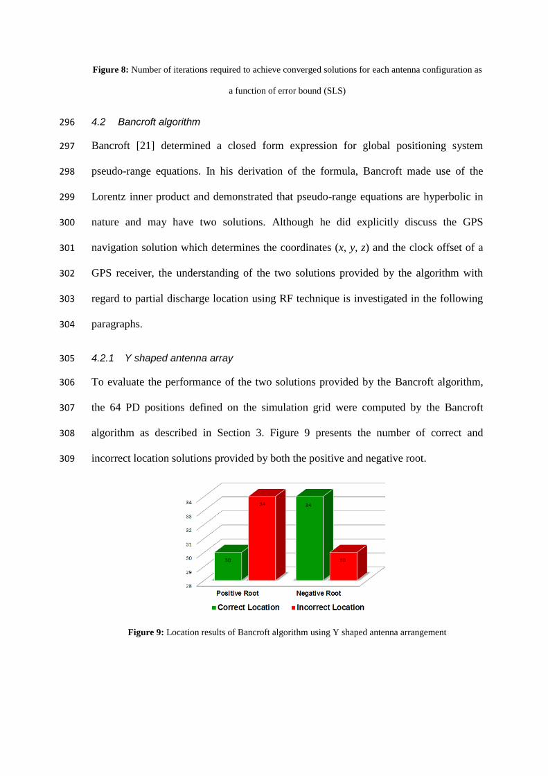
Figure 8: Number of iterations required to achieve converged solutions for each antenna configuration as
a function of error bound (SLS)
4.2 Bancroft algorithm 296
Bancroft [21] determined a closed form expression for global positioning system 297
pseudo-range equations. In his derivation of the formula, Bancroft made use of the 298
Lorentz inner product and demonstrated that pseudo-range equations are hyperbolic in 299
nature and may have two solutions. Although he did explicitly discuss the GPS 300
navigation solution which determines the coordinates (x, y, z) and the clock offset of a 301
GPS receiver, the understanding of the two solutions provided by the algorithm with 302
regard to partial discharge location using RF technique is investigated in the following 303
paragraphs. 304
4.2.1 Y shaped antenna array 305
To evaluate the performance of the two solutions provided by the Bancroft algorithm, 306
the 64 PD positions defined on the simulation grid were computed by the Bancroft 307
algorithm as described in Section 3. Figure 9 presents the number of correct and 308
incorrect location solutions provided by both the positive and negative root. 309
Figure 9: Location results of Bancroft algorithm using Y shaped antenna arrangement

Figure 10: Position of located and non-located PD using Y shaped antenna arrangement and positive root
of the Bancroft algorithm
Based on results of the positive root of the Bancroft algorithm, it can be seen that the 310
algorithm provided accurate positioning to 30 PD locations and 34 incorrect solutions to 311
the remaining PD positions. This demonstrates that the algorithm can only provide 312
partial results to the 64 simulated PD using one of the roots and that the location of 313
these simulated PD require the investigation of both solutions. 314
The exact position of the located and non-located PD is presented in Figure 10, where 315
the green points represent the located positions and the blue points the incorrect 316
solutions. It can be seen from the figure that the positioning results of located and non-317
located PD positions are symmetrical around the antenna central point. This is due to 318
the topology of the Y shaped array, of which the y and z coordinates of antennas 3 and 4 319
are identical. 320
Regarding the location results of the Bancroft algorithm using the negative root, it can 321
be seen from Figure 9 that the algorithm provided 34 accurate PD locations and 30 322
inaccurate PD locations. It should be noted that inaccurate locations using the positive 323
root are found to be located accurately using the negative root and vice versa. This 324
demonstrates that the algorithm can provide accurate locations to the 64 simulated PD 325
positions if valid solutions are selected between both roots. This demonstrates that the 2 326
solutions provided by the algorithm complement each other to provide accurate 327
positioning to the simulated PD. This is because the two hyperbolas intersect at two 328
locations, one that corresponds to the TDOA with correct sign and the other to the 329
TDOA with reversed sign. 330
4.2.2 Square shaped antenna arrangement 331
Using the square antenna arrangement and the positive root, the Bancroft algorithm 332
provided 17 correct locations and 47 incorrect locations (see Figure 11). On the other 333
hand, positioning results using the negative root provided more accurate locations than 334
the positive root, where 52 out of the 64 simulated PD positions located accurately and 335
only 12 PD were located incorrectly. The difference between the correct PD locations 336
using the positive root and the non-located PD using the negative root results from 5 PD 337
positions being located accurately by both roots. 338
Figure 11: Location results of Bancroft algorithm using square shaped antenna arrangement
4.2.3 Discussion 339
Based on the results of the Bancroft algorithm using both positive and negative roots, it 340
can be seen that the algorithm can provide very accurate location results on the 64 341
simulated PD positions. Results also show that the algorithm provided more successful 342
location results when using the negative root instead of the positive root. In addition, 343

location results using the square antenna arrangement were found to be better than the 344
location results when using the Y shaped antenna arrangement. Although location 345
results using the different antenna arrangements differ in terms of the number of 346
successfully located PD using each root, the discrimination between correct and 347
incorrect solutions of the positive and negative root can be carried out using the clock 348
offset parameter. Based on the simulated PD, it was found that the Bancroft algorithm 349
can provide 100% accurate solutions to the simulated PD positions when selecting the 350
cartesian coordinates (x, y, z) corresponding to the lowest clock offset when comparing 351
results of both roots. Validation of this selection process may change when considering 352
noise effects and measurement errors as time offset adjustments cannot be established 353
due to the stochastic nature of the physical PD emission process. 354
Additionally, given only the difference in arrival times of the antennas’ signals, it is 355
difficult to know which solution is correct. The separation between the algorithm's 356
correct and incorrect solutions will depend on the environment where measurements 357
took place. For example, in the case where measurements are carried out in a high 358
voltage power transformer using acoustic sensors attached to the transformer’s housing, 359
discrimination between the different solutions can use the equipment's area spatial 360
volume to limit the search of valid solutions. In the case of open space areas such as 361
electrical substations, if the reference point is at the ground height and the locations of 362
interest are in front of the antenna arrangements, one can limit the search of valid 363
solutions within the positive interval of y and z coordinates. 364
5 Comparison between Iterative and Non-Iterative Algorithms 365
Nonlinear equations of location algorithms which are presented by hyperbolas and 366
distance formulas are commonly solved with iterative algorithms [26]. Results of the 367
iterative algorithm showed that these methods have strong dependencies on different 368

parameters such as the error bound, number of iterations and also initial values which 369
must be provided by the user. On the other hand, non-iterative methods, which do not 370
require iterations and therefore make a fast computation tool, showed that they provide 371
very accurate location results when provided by accurate TDOAs (in this case, 372
theoretical TDOAs were provided). However the selection of correct locations among 373
the two available solutions will depend on the user's experience and ability to 374
discriminate between the different positioning solutions by using for example time 375
restrictions based on the equipment's spatial volume. Table 4 presents some of the 376
advantages and disadvantages of the different location algorithms when applied to PD 377
location. 378
Table 4: Characteristics of the location algorithms
Algorithm Advantages Disadvantages
Iter
ativ
e
(SL
S)
Accurate if provided with well
selected error bound
Accurate if provided with well
selected number of iterations
Accurate if provided with accurate
time of arrival
Depends on number of iterations
Depends on error bound
Depends on initial values
Depends on antenna arrangement
Non
-Ite
rati
ve
(Ban
croft
)
Direct solution
Fast and very accurate
Do not depend on initial values
Possibility of discriminating between
the two solutions (Bancroft method
only)
No indication of converged solutions
Depends on time of arrival accuracy
No way of discriminating between
the two solutions
Provide two different solutions
Depends on antennas arrangement
Using iterative methods, the question which is still raised is: how can the user define a 379
valid error bound and also a valid number of iterations sufficient to provide accurate 380
location results assuming there is no initial values issue (see example of SLS 381
performance at 10-13
error bound in Figure 5)? 382

6 New Approach 383
Based on simulations, it was found that when the error bound is high (e.g. 10-3
error 384
bound), solutions of the location coordinates are often underestimated and the number 385
of iterations required is also low. When the location coordinates of some TDOAs using 386
the iterative results are compared to the location coordinates of the same TDOAs using 387
non-iterative methods, this may show a location mismatch in the case of a non-valid 388
error bound selection and which indicates that the error bound should be decreased. 389
This process should be repeated until matching results are found by both iterative and 390
non-iterative methods. Regarding the selection of a valid number of iterations, this is 391
determined by providing enough iteration values which allow a converged solution 392
based on the matching solutions of both iterative and non-iterative methods to be 393
obtained. Figure 12 summarises the selection process of valid error bounds and number 394
of iterations used by the iterative methods based on the non-iterative method solutions. 395
It should be noted that the iterative methods may sometimes provide a non-converged 396
solutions which may be due to initial values issue or measurement errors. 397

398
Figure 12: Selection of error bound and number of iterations 399
7 Conclusions 400
As a study evaluating the location accuracy of an iterative and non-iterative algorithms 401
as applied to partial discharge measurement, simulations of a range of PD using two 402
different antenna configurations have been presented. 403
By varying the error bounds, it has been shown that the performance of the iterative 404
algorithms as a function of location accuracy can be quantified, despite the nonlinear 405
nature of the location equations. A decrease in the error bound produces more accurate 406
location results while requiring more iterations. The results presented will be useful for 407
a practitioner of condition monitoring of in-service power equipment since it will allow 408
judgement of appropriate levels of required accuracy based on the dimensions of the 409
equipment under surveillance. It will also facilitate estimation of the required 410
computing time to achieve the desired level of location accuracy. The required spatial 411
location accuracy depends on the application. For example, general surveying of 412
equipment on a substation-wide scale may only require a poor to good level of accuracy 413
(1 cm ≤ d ≤ 1 m). This range may also accurately facilitate the location of faults along 414
large equipment sections such as busbars, bushings or power transformers (i.e. larger 415
equipment). 416
Regarding the non-iterative algorithms, it was found that these techniques provide very 417
accurate positioning when provided with precise TDOAs. The accuracy of the non-418
iterative algorithms also depends on the antenna arrangements which influence the 419
number of accurate positions located by the two different roots. The discrimination 420
process between the two different solutions of the non-iterative solutions can be 421
difficult and will depend on the user experience to separate between the two solutions 422
using, for example, time restrictions based on the equipment's spatial volume. 423
A novel approach to select adequate error bounds and number of iterations using results 424
of the non-iterative methods has been established and will contribute considerably to 425
solve some of the iterative method dependencies. 426
In this work, simulations provided an evaluation of the performance of different types 427
of location algorithms based on determined PD locations. This evaluation method gives 428
indications of the essential characteristics of iterative methods and also an insight on the 429
behaviour of non-iterative methods to provide different solutions. The study presented 430
in this paper can benefit electrical utilities, network operators and designers of PD 431
locations systems, as it can be used as a guide to the selection of specific algorithm 432
based on its operation requirements (i.e. computation time, discrimination between 433
solutions, accuracy parameters and their selection process), facilitating more accurate 434
location and diagnosis of incipient faults in high value electrical power equipment. 435

Acknowledgements 436
The work presented in this paper were obtained as part of a financial, academic and 437
technical support provided by Glasgow Caledonian University during the main author 438
PhD studies. 439

References 440
[1] Moore, P. J., Portugues, I. E., and Glover, I. A. “Radiometric location of partial 441
discharge sources on energized high-voltage plant” IEEE Transactions on Power 442
Delivery, 2005, 20, (3), pp 2264-2272 443
[2] Stewart, B. G., Nesbitt, A., and Hall, L. “Triangulation and 3D location 444
estimation of RFI and partial discharge sources within a 400kV substation” 445
Proceedings on IEEE Electrical Insulation Conference, Montreal, Canada , June 446
2009, pp 164-168 447
[3] Tian, Y., Kawada, M., and Isaka, K. “Locating partial discharge source 448
occurring on distribution line by using FDTD and TDOA methods” IEEJ 449
Transactions on Fundamentals and Materials, 2009, 129, (2), pp 89-96 450
[4] El Mountassir, O. Stewart, B, G. McMeekin, S. G. and Ahmadinia, A. 451
“Evaluation of an iterative method used for partial discharge RF location 452
techniques”, 10th
International Conference on Environment and Electrical 453
Engineering, 2011, pp 1-4 454
[5] Coenen, S. and Tenbohlen, S. “Location of PD sources in power transformers by 455
UHF and acoustic measurements” IEEE Transactions on Dielectrics and 456
Electrical Insulation, 2012, 19, pp 1934-1940 457
[6] Steiner, J. P., Reynolds, P. H., and Weeks, W. L. “Estimating the location of 458
partial discharges in cables” IEEE Transactions on Electrical Insulation, 1992, 459
27, pp 44-59 460
[7] Tian, Y., Lewin, P., Davies, A., Sutton, S., and Swingler, S. “Partial discharge 461
detection in cables using VHF capacitive couplers” IEEE Transactions on 462
Dielectrics and Electrical Insulation, 2003, (10), pp 343-353 463

[8] Mardiana, R. and Su, C. Q. “Partial discharge location in power cables using a 464
phase difference method” IEEE Transactions on Dielectrics and Electrical 465
Insulation, 2010, (17), pp 1738-1746 466
[9] Wagenaars, P., Wouters, P. A. A. F., Van der Wielen, P. C. J. M., and Steennis, 467
F. “Influence of ring main units and substations on online partial discharge 468
detection and location in medium voltage cable networks” IEEE Transactions on 469
Power Delivery,2011, (26), pp 1064-1071 470
[10] Meijer, S., Smit, J. J. and Girodet, A. “Estimation of UHF signal propagation 471
through GIS for sensitive PD detection” IEEE International Symposium on 472
Electrical Insulation, 2002, pp 435-438 473
[11] Hu, X., Judd, M. D., and Siew, W. H. “A study of PD location issues in GIS 474
using FDTD simulation”. International Universities Power Engineering 475
Conference, 2010, pp 1-5 476
[12] Hikita, M., Ohtsuka, S., Wada, J., Okabe, S., Hoshino, T., and Maruyama, S. 477
“Study of partial discharge radiated electromagnetic wave propagation 478
characteristics in an actual 154kV model GIS” IEEE Transactions on Dielectrics 479
and Electrical Insulation, 2012, (19), pp 8-17 480
[13] Chiu, M. Y., Liang, K.W., Lee, C. H., Fan, C. L., Cheng, J., and C., L. Y. 481
“Application of MV GIS partial discharge measurement and location” 482
International Conference on Condition Monitoring and Diagnosis, 2012, pp 462-483
465 484
[14] Zheng, B and Bojovschi, A. “Electromagnetic Sensing of Partial Discharge in 485
Air-insulated Medium Voltage Switchgear”, IEEE Power Engineering and 486
Automation Conference, 2012, pp 1-4 487

[15] Judd, M. D., Yang, L., and Hunter, I. B. B. “Partial discharge monitoring for 488
power transformer using UHF sensors. Part 2: Field experience” IEEE Electrical 489
Insulation Magazine, 2005, (21), pp 5-13 490
[16] Tang, Z. G., Chengrong, L. R., Xu, C. ; Wei, W., Jinzhong, L., and Jun, L. 491
“Partial discharge location in power transformers using wideband RF detection” 492
IEEE Transactions on Dielectrics and Electrical Insulation, 2006, (13), pp 1193-493
1199 494
[17] Sinaga, H. H., Phung, B. T., and Blackburn, T. R. “Partial discharge localization 495
in transformers using UHF detection method” IEEE Transactions on Dielectrics 496
and Electrical Insulation, 2012, (19), pp 1891-1900 497
[18] Zhang, X., Tang, J., and Xie, Y. “Taylor-genetic algorithm on PD location” 498
International Conference on High Voltage Engineering and Application, 2008, 499
pp 685-688 500
[19] Miao, P., Li, X., Huijuan, H., Gehao, S., Hu, Y., and Jiang, X. “Location 501
algorithm for partial discharge based on radio frequency (RF) antenna array” 502
Asia-Pacific Power and Energy Engineering Conference, 2012, pp 1-4 503
[20] Y. Lu, X. Tan, X. Hu, “PD detection and localisation by acoustic measurements 504
in an oil-filled transformer”, IEEE Transactions on Science, Measurement and 505
Technology, 2002, (147), pp 81-85 506
[21] O. El Mountassir, B. G. Stewart, S. G. McMeekin and A. Ahmadinia. “Effect of 507
sampling rate on the location accuracy of measurements from radiated RF partial 508
discharges signals” 11th
International Conference on Environment and Electrical 509
Engineering, 2011, pp 891-896 510
[22] Bancroft, S. “An algebraic solution of the GPS equations” IEEE Transactions on 511
Aerospace and Electronic Systems, 1985, (21), pp 56-59 512
[23] Ho, K. M. and Chan, Y. T. “Solution and performance analysis of geolocation 513
by TDOA” IEEE Transactions on Aerospace and Electronic Systems, 1993, 514
(29), pp 1311-1322 515
[24] Yang, M. and Chen, K. H. “Performance assessment of a noniterative algorithm 516
for global positioning system (GPS) absolute positioning” Procceedings of the 517
National Science Council, 2001, (25), pp 102-106 518
[25] Bucher, R. and Misra, D. “A synthesizable VHDL model of the exact solution 519
for three-dimensional hyperbolic positioning system” VLSI Design Journal, 520
2002, (15), pp 507-520 521
[26] Markalous, S., Tenbohlen, S., and Feser, K. “Detection and location of partial 522
discharges in power transformers using acoustic and electromagnetic signals” 523
IEEE Transactions on Dielectrics and Electrical Insulation, 2008, (15), pp 1576-524
1583 525