Embed Size (px)
Citation preview

HAL Id: hal-02467986https://hal.archives-ouvertes.fr/hal-02467986
Submitted on 22 Jan 2021
HAL is a multi-disciplinary open accessarchive for the deposit and dissemination of sci-entific research documents, whether they are pub-lished or not. The documents may come fromteaching and research institutions in France orabroad, or from public or private research centers.
L’archive ouverte pluridisciplinaire HAL, estdestinée au dépôt et à la diffusion de documentsscientifiques de niveau recherche, publiés ou non,émanant des établissements d’enseignement et derecherche français ou étrangers, des laboratoirespublics ou privés.
Quantifying multiple electromagnetic properties in EMIsurveys: A case study of hydromorphic soils in a
volcanic context – The Lac du Puy (France)François-Xavier Simon, Mathias Pareilh-Peyrou, Solène Buvat, Alfredo
Mayoral, Philippe Labazuy, Karim Kelfoun, Alain Tabbagh
To cite this version:François-Xavier Simon, Mathias Pareilh-Peyrou, Solène Buvat, Alfredo Mayoral, Philippe Labazuy, etal.. Quantifying multiple electromagnetic properties in EMI surveys: A case study of hydromorphicsoils in a volcanic context – The Lac du Puy (France). Geoderma, Elsevier, 2020, 361, pp.114084.�10.1016/j.geoderma.2019.114084�. �hal-02467986�

1
Quantifying multiple electromagnetic properties in EMI surveys: a case study of 1
hydromorphic soils in a volcanic context – the Lac du Puy (France) 2
3
François-Xavier Simon1, Mathias Pareilh-Peyrou2, Solène Buvat2, Alfredo Mayoral3, Philippe 4
Labazuy2, Karim Kelfoun2, Alain Tabbagh4 5
1: Institut National de Recherches Archéologiques Préventives, Laboratoire Chrono-6
Environnement, UMR 6249, F-25000, Besançon, France, [email protected] 7
2: Université Clermont Auvergne, CNRS, IRD, OPGC, Laboratoire Magmas et Volcans, F-8
63000 Clermont-Ferrand, France 9
3: CNRS, Université Clermont Auvergne, GEOLAB, F-63000 Clermont-Ferrand, France 10
4: Sorbonne Université, CNRS, EPHE, Métis, 4 place Jussieu F-75252, Cedex 05 Paris, France 11
12
Abstract 13
We used two different loop-loop electromagnetic induction (EMI) devices to determine 14
the 3D geometry and morphology of the pedo-sedimentary filling and underlying basaltic 15
bedrock of a former wetland in a volcanic soil area, the Lac du Puy depression (Auvergne, 16
France). Electrical conductivity (or resistivity) is usually sufficient for environmental and soil 17
science applications, but the local volcanic context of the survey area results in high values of 18
magnetic susceptibility and possible electrical polarization effects. Therefore we investigated 19
the roles of the four properties: electrical conductivity, magnetic susceptibility, magnetic 20
viscosity and dielectric permittivity. We created models using these four properties for the two 21
coil configurations of each device in order to assess the degree to which each of the properties 22
contributed to the recorded electromagnetic signal. The results show that electrical conductivity 23
controls the quadrature component of the secondary field response but that it can be affected by 24
high values of magnetic viscosity, while magnetic susceptibility controls the in-phase 25

2
component. Moreover, the low frequencies imply a limited contribution of dielectric 26
permittivity to the in-phase component, except in the cases of higher permittivity or frequency 27
values or greater inter-coil separation. Based on these observations, we propose a way to map 28
the apparent properties from field measurements. We then carried out a 1D inversion, first by 29
considering the electrical conductivity alone and secondly by taking all the electromagnetic 30
properties into account. The results show that there is a marked contrast in the complex 31
magnetic susceptibility between the sedimentary in-fill and the border of the Lac de Puy 32
depression, (stronger than for the electrical conductivity), and that permittivity is unlikely to 33
have a significant influence. The shape and nature of the sedimentary in-fill was thus 34
considerably refined by the second inversion results based on the three other properties. These 35
data, combined with litho-stratigraphic observations from a previous study, allowed the lateral 36
continuity and geometry of the in-fill to be assessed across the whole basin. Results are also 37
consistent with previous interpretations of the depression as a pseudo-sinkhole, a relatively 38
common morphology in volcanic plateaus. 39
Analysis of the magnetic properties also made it possible to characterize the spatial variation of 40
some key features related to hydromorphic processes, such as clayey granularity and the 41
development of iron oxides/hydroxides. This opens up the possibility for using new methods 42
for rapid spatial and pedological characterization of hydromorphic soils and palaeosoils. 43
44
45
Key words: EMI, VLF frequency range, conductivity, magnetic susceptibility and viscosity 46
mapping, hydromorphic soils, igneous environment 47
48
49
1. Introduction 50

3
Palaeosols and sedimentary layers can provide valuable records of changing Holocene 51
environmental conditions through careful multi-proxy geo-archaeological and paleo-52
environmental analysis (e.g. Dotterweich, 2008; Dreibrodt et al., 2010; Henkner et al., 2017). 53
In this context, frequency domain electromagnetic induction measurements have proven to be 54
a useful tool in the first stages of investigation and prior to coring or trenching (Sudduth et al. 55
2005, Saey et al. 2008, Boaga 2017). These techniques can provide information about 56
electromagnetic properties and make it easier to identify the nature, geometry and thickness of 57
superficial formations and sedimentary bodies containing paleo-environmental information. 58
Moreover, once drilling or trenching has been performed, geophysical observations calibrated 59
with field data can be used to extrapolate stratigraphic or sedimentological observations 60
(Bendjoudi et al. 2002, Hendrickx et al. 2002, Triantafilis and Monteiro Santos 2010, Neely et 61
al. 2016). 62
In the framework of a broader geo-archaeological survey of a small pond, the Lac du 63
Puy, situated at the top of the Puy de Corent in central France (Mayoral et al. 2018a), we used 64
two EMI frequency domain instruments commonly used for environmental and soil studies. 65
First the EMP400 (GSSI Ltd, Nashua, NH, USA) where the inter-coil separation, L, equals 1.2 66
m, and secondly the EM31 (Geonics Ltd, Mississauga, Ontario, Canada) where the inter-coil 67
separation equals 3.66 m, both operating with frequencies close to 10 kHz. Their geometry and 68
operating frequency define the domain of electromagnetic induction used. Here it is the Very 69
Low Frequency (VLF, 3-30 kHz) range, in which, regardless of the type of electromagnetic 70
transmitted signal, the electrical conductivity, σ, is the dominant cause of the underground 71
responses. Consequently, for both instruments, only the apparent electrical conductivity is 72
usually considered (Frischknecht et al. 1991). However, four properties are actually involved 73
(Fig. 1): two electrical (electrical conductivity and dielectric permittivity) and two magnetic 74
(magnetic viscosity and magnetic susceptibility): 75

4
(1) While electrical conductivity represents the global motion of electric charges at the 76
macroscopic scale, another property, permittivity, is required to describe the electrical 77
polarization, which is the oscillations in electrical charge at a microscopic scale (from 78
pore or clay platelet to molecular scales). In the absence of significant changes in salinity 79
or temperature, variations in both properties reflect variations in the granularity, mainly 80
the clay content, or in the soil water content. Both properties can be found in the 81
Maxwell-Ampere equation in the expression, ri 0 , where ω is the angular 82
frequency, ε0 the vacuum permittivity, εr the relative permittivity and 1i . The 83
relative weighting of the permittivity depends on the frequency: in the low frequency 84
(EMI) domain it can only be strong if εr is strong (Benech et al., 2016, Simon et al. 85
2019). 86
(2) As the acquisition of induced magnetization by a mineral grain is not immediate, there 87
is a delay in acquisition or loss of the induced magnetization (Dabas and Skinner 1993, 88
McNeill 2013, Jordanova 2017). This delay is taken into account by considering that 89
the magnetic susceptibility is a complex quantity, quph i , where κph is the in-90
phase magnetic susceptibility (hereafter simply called magnetic susceptibility) and κqu 91
is the magnetic viscosity. The magnetic viscosity depends on the size of the magnetic 92
grains. It is strong for small single domain magnetite grains (in the [10 – 30 nm] 93
equivalent diameter range), small for larger single domain grains (around 1 µm) and 94
once again strong for large multi-domain grains (20 µm and greater). These magnetic 95
properties can be used jointly to describe the degree of pedogenesis, as the quantity and 96
size of magnetic grains are directly linked to redox processes that affect iron 97
oxides/hydroxides. Although the presence of organic matter affects these processes 98
(Cuenca Garcia et al. 2019), the content of iron oxides of the parent rock plays a key 99

5
role in the magnitude of soil magnetic susceptibility. In general, high magnetic 100
susceptibility would be expected for basaltic rocks (1000 to10000 10-5 SI). 101
Frequency domain EMI apparatuses with a coil spacing of greater than 3 m and a frequency 102
lower than 30 kHz - such as the EM31- have been used in a wide variety of environmental 103
studies since 1979 (de Jong et al. 1979). Furthermore, over 200 papers have been published 104
using the conductivity measurements obtained with this device (Doolittle and Brevik 2014), but 105
to the best of our knowledge only very few studies look at the other EM property measurements 106
for this instrument. On the other hand, in the field of archaeological prospection, where the 107
separation between the coils remains limited, less than two meters, it has been noted that the 108
magnetic properties play an important part in ground response (Tite and Mullins 1970, Scollar 109
et al. 1990, Simon et al. 2015, De Smedt 2014). 110
In the Puy de Corent pond, the presence of basaltic rocks (basanite) underlying the 111
depression is of particular interest in the study of magnetic properties and electrical polarization 112
phenomena. Such rock types usually contain a high content of stable single domain magnetic 113
grains with high susceptibility (Grison et al. 2015), very low viscosity and significant electrical 114
polarizability. Therefore, the purpose of our work was to investigate the four measurable 115
electromagnetic properties rather than using electrical conductivity alone, and to assess their 116
relative abilities to improve interpretation of three-dimensional sedimentary infill (Triantafilis 117
et al., 2013a, Triantafilis et al., 2013b), well documented in Mayoral et al. 2018a but mainly 118
based on direct and spatially limited stratigraphic observations. This non-intrusive approach 119
provides benefits in terms of both time and resources. The raw data is collected by the two 120
instruments and then inverted using point by point 1D modelling, considering first the electrical 121
conductivity alone, and then incorporating the electrical conductivity, the complex magnetic 122
susceptibility and the relative dielectric permittivity in a second round of modelling. 123
124
6
2. Material and methods 125
2-1. Study area and Stratigraphy 126
The study site is located on top of the Puy de Corent (621 m.a.s.l.), a volcanic plateau 127
dominating the calcareous Limagne Plain in central France. The plateau has been shaped by 128
erosion and topographic inversion of a 3 million year-old scoria cone and an associated basaltic 129
lava flow formed during the Pliocene volcanism of the Massif Central (Greffier, et al., 1980; 130
Nehlig et al., 2003). In the quasi-flat lower part of the plateau, a small circular depression of 131
circa. 2 ha forms a wetland representing a drained pond (Fig. 2). This depression was formerly 132
interpreted as being a secondary crater, but is more likely a pseudo-sinkhole, caused by 133
subsidence phenomena affecting the basaltic lava flow, likely triggered by dissolution of 134
underlying Oligocene sedimentary rocks including marls, limestones and gypsum (Mayoral et 135
al., 2018). Litho-stratigraphic features of the Lac du Puy have already been described in detail 136
in previous work (Mayoral et al. 2018), and are summarized here in Figure 2. The bedrock is 137
basaltic and is formed of the Puy de Corent lava flow. The sedimentary in-fill of the basin is 138
mainly clayey and can reach a thickness of up to 1.8 or 2 m. The lower stratigraphic units have 139
a clay matrix which is very rich in coarse volcanic material (sand to gravel), resulting from 140
detrital input from the plateau and local bedrock weathering and disaggregation. The middle 141
stratigraphic units are dominated by massive, heavy clays which have undergone various phases 142
of pedogenesis since the Neolithic, with dominant hydromorphic features (gleyic and vertic 143
features) and rare coarse particles. The upper units are mainly clayey loams including several 144
basaltic fragments and pottery sherds, and show Roman to present-day soil development. 145
Magnetic susceptibility was measured on two different cores along a trench and is summarized 146
as an average per sedimentary unit. Susceptibility values were measured with the single 147
frequency MS2-E (Bartington Ltd, UK, 1cm spatial resolution, 2 kHz) on the fine soil fraction. 148

7
This resulted in relatively low susceptibility values (less than 50.10-5 SI), not taking into 149
account the effect of the basaltic and sherd fragments. 150
2-2. Devices and survey conditions 151
Two different EMI devices were used on the study site. The EMP400 operates at three 152
frequencies below 16 kHz (5, 8 and 15 kHz were selected). This instrument has one transmitting 153
coil and one receiving coil at a distance of L=1.21 m from the transmitting coil. The coils are 154
coplanar, and measurements can be made in either the HCP (horizontal coplanar) or the VCP 155
(vertical coplanar), which is configured by rotating the instrument itself. The depths of 156
investigation for the EMP400 differ between the HCP and VCP, and for the electrical and 157
magnetic properties (Tabbagh 1986b). For the electrical properties, it is generally 0.8L in VCP 158
and 1.5L in HCP, whereas for the magnetic ones the distances are 0.6L in VCP and 0.2L in 159
HCP, with a change in the sign of the response for a clearance h=0.38 L. 160
The second device, the EM31, has a coplanar configuration, a 3.66 m inter-coil 161
separation and a single frequency of 9.8 kHz. The operator can hold the instrument at shoulder 162
height with h=1 m clearance above the ground surface. It can also be pulled using a trolley at a 163
lower clearance. The depths of investigation follow the same general guidelines for L as for the 164
EMP400. 165
The Lac du Puy area was surveyed with the two instruments in both HCP and VCP 166
configurations, in combination with a GNSS positioning system with a sub-decimetric accuracy 167
in order to locate the instrument operator precisely. A profile was collected every two meters 168
with a frequency of data collection of 1 Hz for the EM31 and 10 Hz for the EMP400. Data for 169
both instruments and configurations were collected on October 2015, resulting in eight different 170
independent sets of data: EM31 in HCP, EM31 in VCP, EMP400 in HCP for 5, 8 and 15 kHz 171
and EMP400 in VCP for 5, 8 and 15 kHz. Each was resampled with the same 2 m x 2 m grid 172

8
meshing in order to enable simultaneous interpretations and inversions using these different 173
sets. 174
175
2-3. 1D forward modelling 176
We present here the 1D forward modelling, which takes the four electromagnetic properties 177
into account (see also Ward and Homann 1988). It allows us to define the apparent properties 178
when the ground is assumed to be homogeneous, and to inverse for properties and thicknesses 179
of the successive layers when a multi-layer model is considered. 180
For horizontal coplanar (HCP), where the transmitter is a vertical magnetic dipole, Mz, 181
located at (0, 0, -h) and the receiver a small coil located at (0, L, -h), 182
0
0
22 )()(4
0
dLJeRM
Hhu
vz
z (1) 183
For vertical coplanar (VCP), where the transmitter is a horizontal magnetic dipole, Mx, 184
located at (0, 0, -h) and the receiver a small coil located at (0, L, -h), 185
0 0
1
2
1
0
22
0 )()(1
)()(4
0
0
dLJ
eR
LdLJeR
MH
hu
hu
H
x
x (2) 186
In these expressions J0 and J1 are the Bessel’s function of the first kind, 2
0
2
0 u with187
2
00
2
0 , and
1
0
0
1
0
0
0
)(
Yu
Yu
uRv
, Y1 being recursively calculated by starting at the top 188
of the deepest layer, N, by N
NN
uY
and using the formula:
iii
i
i
ii
i
i
i
i
i
i
euYu
euu
Yu
Y
tanh
tanh
1
1
. In 189
this formula, ei is the thickness of the ith layer, and 22
iiu with 22 iiiii i 190
and 1i . 191

9
)()()( 2
0
2
01 vH RuRR . The function 𝑅𝐻(𝜆) is calculated by
1
0
0
1
0
0
0
)(
Zi
u
Zi
u
uRH
, Z1 192
being recursively calculated by starting at the top of the deepest layer by NN
NN
i
uZ
193
and using the formula:
iii
ii
i
ii
ii
i
i
ii
i
i
euZi
u
eui
uZ
i
uZ
tanh
tanh
1
1
. To get results which are 194
independent of the transmitted power, the secondary field expressions are usually normalized 195
by the primary amplitude, Hp=M/(4πL3) and the measurements are expressed in terms of Hs/Hp 196
, in ppm (parts per million) or in ppt (parts per thousand) depending on the device manufacturer 197
(ppm for the EMP400 and ppt for the EM31, 1ppt=1000 ppm). 198
To illustrate the physical meaning of these complex analytic expressions by showing 199
the influence of any property or instrument parameter, approximations (Thiesson et al. 2014) 200
can be calculated based on the range of values of the different properties. The static 201
approximation ( 0 ) establishes that the ratio of the secondary field to the primary field for 202
a coplanar instrument (HCP or VCP) located at h=0 clearance above the surface would be 203
2
quph
p
si
H
H . This suggests that the magnetic susceptibility response would be in-phase, 204
the viscosity response in quadrature and their dependence on frequency and coil separation 205
limited. Furthermore, the Low Induction Number (LIN) approximation, 12 L , which 206
corresponds, if µ=µ0 and h=0, to 4
2
0 Li
H
H
p
s suggests that the conductivity effects would 207
mainly be in quadrature and proportional to the conductivity, the frequency and the square of 208
the coil separation (this approximation is the one commonly used by most instrument 209
manufacturers to define ECa). 210
10
If we take into account the permittivity, this last approximation becomes211
44
22
00
2
0 LLi
H
H r
p
s , which suggests that the permittivity response would be first 212
order in-phase and would drastically increase with the frequency and coil separation. 213
Consequently, the in-phase response can be dependent on both the magnetic susceptibility and 214
the relative permittivity. Note also that even if the displacement currents are negligible in 215
comparison with conduction ones, ri 0 , the permittivity response may be significant 216
in comparison with the susceptibility response. 217
218
2-4. Instrument calibration and sensitivity analysis 219
At each geometrical configuration and frequency an instrument measures two quantities, 220
the in-phase and quadrature responses, and it is important to understand the influence of each 221
of the four properties (electrical conductivity (or Eca), dielectric permittivity, magnetic 222
susceptibility (or Msa) and magnetic viscosity) on these responses. 223
To assess this, the calculated responses, as a function of each of the four properties, are 224
expressed by the ratios of the secondary field to the secondary field of a reference ground, where 225
σ=0.01 Sm-1, εr=200, κph=100 10-5 SI and κqu =0.06κph. In this trial each property is varied from 226
0.1 to 10 times that of the value used in the reference case value. Figure 3 presents the in-phase 227
modelled responses for the EMP400, and Figure 4 those for the quadrature situation for both 228
configurations and each frequency. For the low-frequency instrument, the influence of 229
permittivity is negligible, as illustrated by the flat curve in Figure 3 at all configurations and 230
frequencies. The magnetic susceptibility dominates the in-phase response with a linear 231
dependence (Fig. 3), and conductivity controls the quadrature responses with a quasi-linear 232
dependence (Fig. 4). These characteristics are in complete agreement with all that has already 233
been published (McNeill 1980, Tabbagh 1986a). However, a precise interpretation needs to 234

11
take the effect of the conductivity on the in-phase response into consideration, which increases, 235
but not in direct proportion to the conductivity (Fig. 3), and the effect of the magnetic viscosity 236
on the quadrature response (Fig. 4). The procedure to determine these properties is presented in 237
Simon et al. (2015). 238
No drift has been observed for the EMP400 (but the temperature changes during the 239
acquisition remained limited). A major drawback of the raw data sets is that they first require 240
the determination of the zero offsets or signal shifts. For in-phase components such shifts are 241
mainly caused by mechanical deformations that modify the direct influence of the primary field, 242
but, surprisingly, offsets also exist in quadrature. For each configuration, this step was achieved 243
by a trial and error process to overcome this problem. In quadrature, the different apparent 244
conductivity values, calculated at each frequency and by considering the differences between 245
each frequency pair, must be as close as possible to each other and positive, while the magnetic 246
viscosity must be positive (Simon et al. 2015). In-phase, the different susceptibility values must 247
be as close as possible and positive. The zero offsets are given in Table 1. 248
Following the same approach as for the EMP400, Figures 5 and 6 show the evolution of the 249
ratio of the in-phase and quadrature secondary fields to those of the reference case for the EM31, 250
in which each property varies from 0.1 to 10 times the value used in the reference case. The 251
dependence of the quadrature response on magnetic viscosity is, in this case (h=1m), quasi null 252
(Fig. 6); therefore, the conductivity determination can be directly achieved with this component 253
at a single frequency. The in-phase component is sensitive to conductivity, permittivity and in-254
phase magnetic susceptibility (Fig. 5), the permittivity response is illustrated by a quasi-flat 255
curve for all configurations and clearance; it is significantly smaller than those of the 256
susceptibility and conductivity. Determination of the apparent properties thus follows a two-257
step approach: (1) determination of the apparent conductivity using the quadrature response; 258
(2) taking into account the in-phase electrical conductivity response, determination either of the 259

12
apparent magnetic susceptibility or of both the permittivity and the susceptibility if both HCP 260
and VCP configurations are available. This last step follows the linear process described in 261
Benech et al. (2016). 262
With EM31, no zero offset correction is necessary for the quadrature part of the signal 263
because of the good field calibration of the device achieved by the manufacturer and of the 264
large coil spacing which increases the signal/noise ratio. On the other hand, the zero offset 265
corrections for the in-phase part of the signal must be evaluated (this component is used in metal 266
detection). Here, following the same the calibration protocol as for the EMP400, in-phase signal 267
offsets were established at 56 ppt for HCP (56000 ppm) and 64 ppt (64000 ppm) for VCP by a 268
trial and error process. These high values correspond to a significant uncertainty regarding the 269
exact offset value, but not for the spatial variations of the properties. 270
271
3- Results 272
3-1. Apparent property maps 273
Each apparent property is defined here as the property of homogeneous flat ground that 274
would give the same response as that obtained with the considered instrument. 275
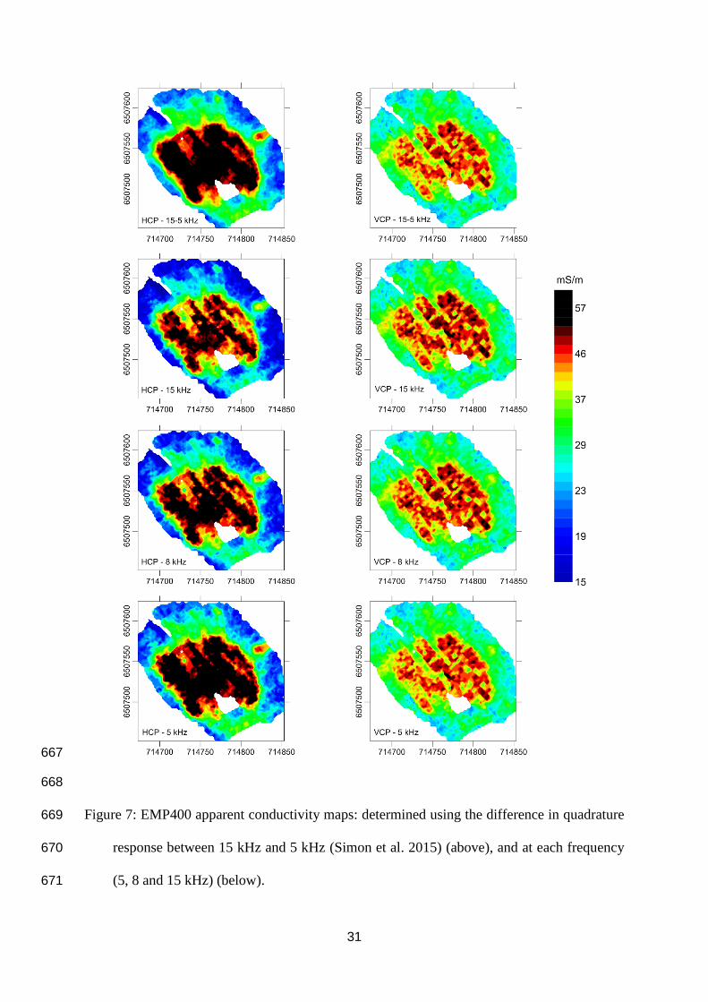
The maps resulting from the EMP400 measurements are presented in Figure 7 for the 276
apparent conductivity, and in Figure 8 for the apparent magnetic susceptibility. As the magnetic 277
viscosity, the conductivity and the depth of investigation are independent of the frequency, the 278
difference in quadrature responses between the 15 kHz and 5 kHz frequencies allowed us to 279
remove the magnetic viscosity effect (Simon et al. 2015). To determine the electrical 280
conductivity we thus compared these differences to the corresponding theoretical reference 281
curves calculated from equations (1) for HCP, or (2) for VCP. We also used theoretical 282
reference curves for each frequency to determine the electrical conductivity using the 283

13
quadrature responses. Using this electrical conductivity value, it is then possible to extract the 284
magnetic viscosity value, which is shown for the VCP and HCP configurations in Figure 9. 285
As illustrated in Figure 7, the maps of electrical conductivity at the different frequencies 286
show identical results, in complete agreement with the values of the Induction Number that 287
establish the similarity in depths of investigation. This result corroborates the solution adopted 288
for the computation of magnetic viscosity. The HCP and VCP maps for apparent conductivity 289
are also very similar. The HCP configuration exhibits a greater range of values, and lower 290
values at the edge of the depression, in agreement with an investigation at greater depth. In the 291
center, the values are higher than 0.04 S.m-1 and, as expected, confirm the clayey nature of the 292
filling and clearly delineate the topographic trough. 293
For magnetic properties, reference curves deduced from equations (1) and (2) are used 294
to determine the apparent magnetic susceptibility, taking into account the estimated electrical 295
conductivity at each point. The HCP and VCP susceptibilities are globally very high, between 296
300 and 3,800 10-5 SI, in agreement with the presence of a basaltic rock substratum (Trigui and 297
Tabbagh 1990). The differences between results for the three frequencies are small, as predicted 298
by the theory. The strong similarity confirms the efficiency of the correction of the induction 299
effect on the in-phase signal for HCP and VCP configurations, respectively. However, the 300
sediment in-fill has lower susceptibility values than the border, at around 700 10-5 SI. The 301
horizontal delineation is in complete agreement with that of the conductivity. The magnetic 302
viscosity is relatively low and its lateral distribution differs from that of the susceptibility. In 303
HCP the magnetic viscosity (depth of investigation of 0.2 L) is higher than in VCP (depth of 304
investigation: 0.6 L) which suggests that it is stronger for the superficial layer of the depression. 305
This observation is in complete agreement with the field observations. The uppermost 45-50 306
centimeters, of slightly varying thickness, contain many sherds and are very different to the 307
deeper layer (Mayoral et al. 2018a). The ratio ph
qu
values, being higher than 4% inside the 308

14
topographic trough and lower than 1% at the border, confirm that the basalt mainly contains 309
stable single-domain magnetic grains (high susceptibility and low magnetic viscosity) while the 310
in-fill has been enriched by pedogenic processes - such as redoximorphic processes or alteration 311
of mineral grains (Mayoral et al. 2018) - into smaller single-domain grains closer in volume to 312
the superparamagnetic range (Maher and Taylor 1988). By comparison, a ratio of 6% or more 313
is expected for common non-hydromorphic soils (Dabas and Skinner 1993). As only a single 314
frequency device (MS2-E) was used on the laboratory soil sample measurements, no direct 315
comparison in terms of frequency variation for the susceptibility can be carried out for this field 316
observation. 317
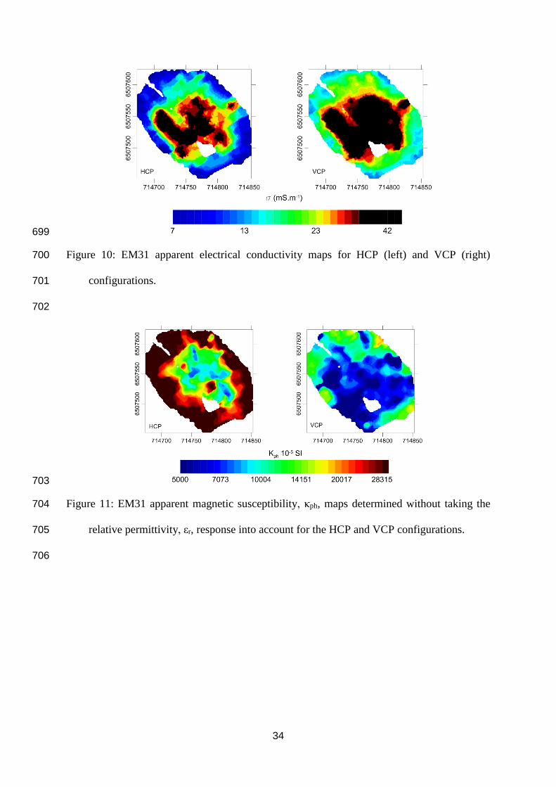
HCP and VCP conductivity maps obtained from the EM31 quadrature signal (Figure 318
10) confirm the horizontal distribution shown by the EMP400 maps. As expected, given that 319
the investigation depth is greater, the conductivity values are about one and a half times lower 320
than for the EMP400. 321
For the in-phase signal, due to the longer coil separation, the effects of both the magnetic 322
susceptibility and the relative permittivity should be considered. The raw data variability is 323
presented in Table 2. The sensitivities of EM31 to the homogeneous ground properties are given 324
in Table 3. The lower sensitivity to κph of the HCP response is due to the instrument’s clearance, 325
h=1 m, because this elevation is close to the change in sign which occurs in the HCP 326
configuration for magnetic responses (at h=1.39 m for a coil separation of 3.66 m). If we 327
calculate the apparent magnetic susceptibility from the in-phase responses without considering 328
the relative permittivity, the discrepancy between HCP and VCP results is marked (Figure 11): 329
the spatial distributions are significantly different with a higher dynamic in HCP (in the range 330
7,500 to 50,000 10-5 SI), and a lower dynamic in VCP (in the range 2,500 to 18,000 10-5 SI). 331
As potentially imperfect offset corrections would increase this effect, the significant difference 332
15
between the two configurations can probably be explained by the sensitivity to susceptibility 333
distribution in relation to the depth. 334
The maps presented in Figure 12 show the results with both the permittivity and the 335
susceptibility taken into account to define the homogeneous half-space properties using both 336
HCP and VCP in-phase values (Benech et al. 2016). In these apparent property maps, the 337
susceptibility variations remain similar to those observed in Figure 11, whereas the permittivity 338
variations are huge, with a 140,000 interquartile deviation and a big gap for the zero offset. The 339
range of values looks unlikely and it can only be assumed that the basalt border has lower values 340
than the sedimentary in-fill in the depression. The high susceptibility values agree with the 341
presence of a basaltic substratum underlying the sedimentary in-fill and are logically greater 342
than the values delivered by the EMP400. The permittivity values logically result from the low 343
sensitivity presented in Table 3. Considering the high magnetic context and the unlikely 344
apparent permittivity values, the intervention of a permittivity response looks unrealistic. This 345
conclusion will be reconsidered later on when considering a layered terrain. 346
From the apparent property mapping, it can be seen that the filling is more conductive 347
and possibly more polarizable than the surrounding basalt. Its conductivity indicates that it is 348
dominated by fine particles. It has a lower magnetic susceptibility with respect to the 349
surrounding weathered basalt, but a higher magnetic viscosity. Taking all this into account, the 350
electromagnetic properties can provide an accurate description of magnetic behavior in addition 351
to the electrical properties. We are then able to describe not only the clay filling of the 352
depression but also some pedogenetic phenomena, and even provide further details about the 353
lateral and horizontal variations in the hydromorphic soils in a volcanic context, which is poorly 354
revealed by a single electrical conductivity mapping based approach. 355
356
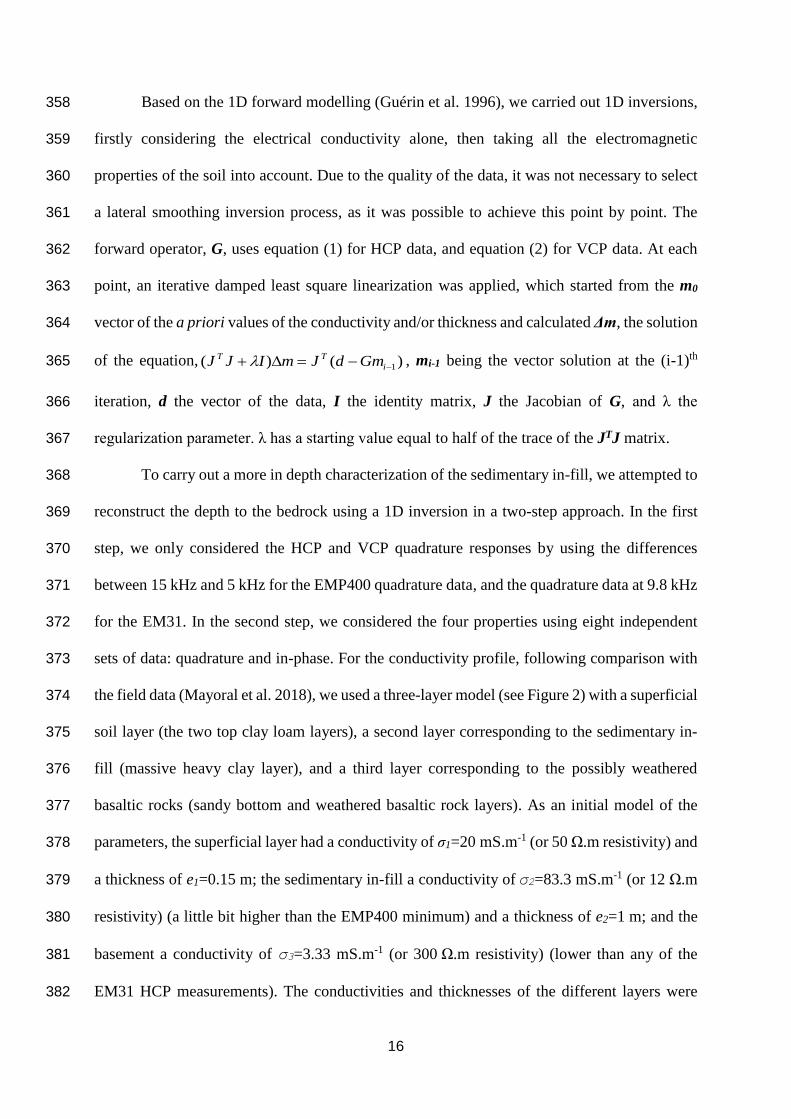
3-2 1D inversion processing using quadrature data 357
16
Based on the 1D forward modelling (Guérin et al. 1996), we carried out 1D inversions, 358
firstly considering the electrical conductivity alone, then taking all the electromagnetic 359
properties of the soil into account. Due to the quality of the data, it was not necessary to select 360
a lateral smoothing inversion process, as it was possible to achieve this point by point. The 361
forward operator, G, uses equation (1) for HCP data, and equation (2) for VCP data. At each 362
point, an iterative damped least square linearization was applied, which started from the m0 363
vector of the a priori values of the conductivity and/or thickness and calculated Δm, the solution 364
of the equation, )()( 1 i
TT GmdJmIJJ , mi-1 being the vector solution at the (i-1)th 365
iteration, d the vector of the data, I the identity matrix, J the Jacobian of G, and λ the 366
regularization parameter. λ has a starting value equal to half of the trace of the JTJ matrix. 367
To carry out a more in depth characterization of the sedimentary in-fill, we attempted to 368
reconstruct the depth to the bedrock using a 1D inversion in a two-step approach. In the first 369
step, we only considered the HCP and VCP quadrature responses by using the differences 370
between 15 kHz and 5 kHz for the EMP400 quadrature data, and the quadrature data at 9.8 kHz 371
for the EM31. In the second step, we considered the four properties using eight independent 372
sets of data: quadrature and in-phase. For the conductivity profile, following comparison with 373
the field data (Mayoral et al. 2018), we used a three-layer model (see Figure 2) with a superficial 374
soil layer (the two top clay loam layers), a second layer corresponding to the sedimentary in-375
fill (massive heavy clay layer), and a third layer corresponding to the possibly weathered 376
basaltic rocks (sandy bottom and weathered basaltic rock layers). As an initial model of the 377
parameters, the superficial layer had a conductivity of σ1=20 mS.m-1 (or 50 Ω.m resistivity) and 378
a thickness of e1=0.15 m; the sedimentary in-fill a conductivity of σ2=83.3 mS.m-1 (or 12 Ω.m 379
resistivity) (a little bit higher than the EMP400 minimum) and a thickness of e2=1 m; and the 380
basement a conductivity of σ3=3.33 mS.m-1 (or 300 Ω.m resistivity) (lower than any of the 381
EM31 HCP measurements). The conductivities and thicknesses of the different layers were 382
17
tested and it was observed that the parameters of the uppermost layer had only a very limited 383
influence. EMI inversions were also subject to so-called ‘cases of equivalence’: in the case of 384
a conducting layer between two more resistive ones (H type for vertical electrical soundings), 385
the conductive layer can be exchanged for any other layer with the same
3
2
e ratio (Guérin et 386
al. 1996). Finally, by allowing only e2 and σ1 to vary, and keeping the other parameters fixed, 387
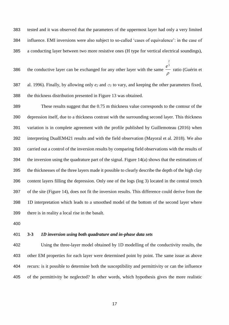
the thickness distribution presented in Figure 13 was obtained. 388
These results suggest that the 0.75 m thickness value corresponds to the contour of the 389
depression itself, due to a thickness contrast with the surrounding second layer. This thickness 390
variation is in complete agreement with the profile published by Guillemoteau (2016) when 391
interpreting DualEM421 results and with the field observation (Mayoral et al. 2018). We also 392
carried out a control of the inversion results by comparing field observations with the results of 393
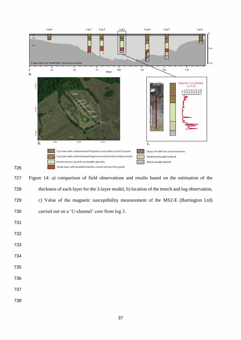
the inversion using the quadrature part of the signal. Figure 14(a) shows that the estimations of 394
the thicknesses of the three layers made it possible to clearly describe the depth of the high clay 395
content layers filling the depression. Only one of the logs (log 3) located in the central trench 396
of the site (Figure 14), does not fit the inversion results. This difference could derive from the 397
1D interpretation which leads to a smoothed model of the bottom of the second layer where 398
there is in reality a local rise in the basalt. 399
400
3-3 1D inversion using both quadrature and in-phase data sets 401
Using the three-layer model obtained by 1D modelling of the conductivity results, the 402
other EM properties for each layer were determined point by point. The same issue as above 403
recurs: is it possible to determine both the susceptibility and permittivity or can the influence 404
of the permittivity be neglected? In other words, which hypothesis gives the more realistic 405

18
results with respect to the geological/pedological context and the external information available 406
describing the depression as having an irregular base shaped into several alteration zones? 407
When the permittivity is neglected, the magnetic susceptibility obtained for the second 408
layer by using four sets of in-phase data is presented in Figure 15. The permittivity for the three 409
layers is fixed at an ordinary value of: εr1=εr2=εr3=200, and with κph1=500 10-5 SI and κph3=2000 410
10-5 SI. The map is in agreement with the apparent susceptibility maps in terms of the lateral 411
distribution and the parameter’s magnitude (Figures 8 and 11). 412
Figure 16 presents the results for the case where the permittivity of the second layer is 413
variable. These results are obtained with εr1=εr3=2000 but are practically independent of the 414
first and third layer fixed permittivity values. The susceptibility is reduced by a factor close to 415
two and, again, the permittivity values are very high and unrealistic. For a permittivity of 106 416
(median value obtained), the quantity ωεrε0 would equal 0.54 Sm-1, seven times greater than the 417
conductivity itself (83 mS.m-1). Considering this extremely high and unlikely estimated range 418
of values of dielectric permittivity, the second hypothesis, where the variations of the 419
permittivity are not characterized for the EMP400 and EM31 instruments, and where the in-420
phase results correspond to magnetic susceptibility only, must be adopted. 421
A comparison with the susceptibility observed at a scale of 1 cm in the cores (‘U-422
Channel’ cores), which is summarized in Figure 14, shows a significant discrepancy between 423
the magnitude of inverted in-field susceptibility values and the laboratory ones (MS2-E) for the 424
in-fill of the depression. This discrepancy is explained if one considers that the presence of 425
basalt gravels and pebbles (with around 12000 10-5 SI susceptibility) is taken into account by 426
in-field measurements rather than laboratory one on the cores. These coarse particles would 427
correspond to one fourth or one fifth of the sediment volume at a metric scale. 428
429
4 Conclusion 430

19
This case study confirms the relevance of this type of light EMI apparatus for the rapid 431
exploration of superficial sedimentary/pedological formations, and will increase the reliability 432
of future sediment sampling at the Lac du Puy. Two different single receiver instruments were 433
used, although a multi-receiver/multi-frequency apparatus would produce the same results and 434
be easier to use. 435
The highly magnetic context due to the basaltic substrate led us to look at the in-phase 436
measurements and try to describe the magnetic susceptibility and magnetic viscosity of the in-437
fill. This process is more common for shorter separation instruments, but nothing has yet been 438
published about this usage for the EM31. The superficial soil and the depression in-fill have a 439
lower magnetic susceptibility and a higher magnetic viscosity than the surrounding weathered 440
basalt and their spatial distribution is slightly different to that of the sediment thickness. Due to 441
the improbable magnitude of the inverted permittivity results, no role can be attributed to the 442
dielectric permittivity variations and the full signal can be attributed to the complex magnetic 443
susceptibility and electrical conductivity. Further studies should be done in the future to assess 444
the effect of permittivity on the in-phase EM31 signal. In this volcanic substrate case study, 445
magnetic susceptibility responses outweigh the electrical polarization when using the EM31. It 446
would be worth doing further investigations in order to assess the potential for this type of 447
instrument in other environments, such as coastal areas or salt-rich soils. 448
In conjunction with the field characterization of the sedimentary accumulation, 449
measurements of the quadrature and in-phase components of the Hs/Hp ratio using the HCP 450
and VCP configurations for both instruments provided a clear description of the conductivity 451
variations. It enabled the Lac du Puy sedimentary in-fill to be identified, by mapping the shape 452
and morphology of the bedrock, lending support to the hypothesis that the depression is a 453
pseudo-sinkhole (Mayoral et al 2018a). 454

20
The analysis of a combination of magnetic properties allowed the 3D morphology of the 455
sedimentary in-fill to be determined across the basin, and provided stratigraphic and 456
sedimentological information. In addition, selected magnetic properties provided information 457
on the spatial variation of some key features related to hydromorphic processes, in particular 458
clayey granularity and the development of iron oxides/hydroxides. These findings, which will 459
be further tested and refined in other parental rocks, could provide new means of rapid spatial 460
and pedological characterization of hydromorphic soils and palaeosoils, with useful 461
applications for palaeoenvironmental studies. 462
463
464
References 465
Benech C., Lombard P., Réjiba F., Tabbagh A., 2016. Demonstrating the contribution of 466
dielectric permittivity to the in-phase EMI response of soils: example of an archaeological site 467
in Bahrain. Near Surface Geophysics, 14-4, 337-344. 468
Bendjoudi H., Weng P., Guérin R., Pastre J. F., 2002. Riparian wetlands of the middle reach of 469
the Seine river (France): historical development, investigation and present hydrologic 470
functioning, a case study. Journal of Hydrology, 263, 131-155. 471
Boaga J., 2017. The use of FDEM in hydrogeophysics: A review. Journal of Applied 472
Geophysics, 139, 36-46. 473
Cuenca Garcia C., 2019. Soil geochemical methods in archaeo-geophysics: Exploring a 474
combined approach at sites in Scotland, Archaeological Prospection, 26,1, 57-72. 475
Dabas M., Skinner J., 1993. Time domain magnetization of soils (VRM), experimental 476
relationship to quadrature susceptibility. Geophysics, 58, 326-333. 477

21
de Jong E., Ballantyne A. K., Cameron D. R., Read D. W. L., 1979. Measurement of Apparent 478
Electrical Conductivity of Soils by an Electromagnetic Induction Probe to Aid Salinity Surveys. 479
Soil Science Society of America Journal, 43-4, 810-812. 480
De Smedt P., Saey T., Meerschman E., De Reu J., De Clercq W., Van Meirvenne M., 2014. 481
Comparing apparent magnetic susceptiblity measurements of a multi-receiver EMI sensor with 482
topsoil and profile magnetic susceptibility data over weak magnetic anomalies, Archaeological 483
prospection, 21, 2, 103-112 484
Doolittle J. A., Brevik E. C., 2014. The use of electromagnetic induction techniques in soils 485
studies. Geoderma, 223-225, 33-45. 486
Dotterweich M., 2008. The history of soil erosion and fluvial deposits in small catchments of 487
central Europe: Deciphering the long-term interaction between humans and the environment 488
— A review. Geomorphology, 101, 192–208. 489
Dreibrodt S., Lomax J., Nelle O., Lubos C., Fischer P., Mitusov A., Reiss S., Radtke U., 490
Nadeau M., Grootes P. M., & Bork H.-R., 2010. Are mid-latitude slopes sensitive to climatic 491
oscillations? Implications from an Early Holocene sequence of slope deposits and buried soils 492
from eastern Germany. Geomorphology, 122, 351–369. 493
Frischknecht F. C., Labson V. F., Spies B. R., Anderson W. L., 1991. Profiling Methods Using 494
Small Sources. In Electromagnetic Methods in Applied Geophysics: Volume 2, Application, 495
Parts A and B, M. N. Nabighian ed., SEG, pp105-270. 496
Grison H., Petrovsky E., Stejskalova S., Kapicka A., 2015. Magnetic and geochemical 497
characterization of Andosols developed on basalts in the Massif Central, France, Geochemistry, 498
Geophysics, Geosystems, 16, 1348–1363, doi:10.1002/2015GC005716. 499
Guérin R., Méhéni Y., Rakotondrasoa G., Tabbagh A., 1996. Interpretation of Slingram 500
conductivity mapping in near-surface geophysics: using a single parameter fitting with 1D 501
model. Geophysical Prospecting, 44, 233-249. 502

22
Greffier G., Restituito J., & Héraud H., 1980. Aspects géomorphologiques et stabilité des 503
versants au sud de Clermont-Ferrand. Bulletin de liaison du Laboratoire des Ponts et 504
Chaussées, 107, 17–26. 505
Guillemoteau J., Simon F.-X., Lück E., Tronicke J., 2016. 1D sequential inversion of portable 506
multi-configuration electromagnetic induction data. Near Surface Geophysics, 14, 411-507
420.Henkner J., Ahlrichs J. J., Downey S., Fuchs M., James B. R., Knopf T., Scholten T., 508
Teuber S., Kühn P., 2017. Archaeopedology and chronostratigraphy of colluvial deposits as a 509
proxy for regional land use history (Baar, southwest Germany). Catena, 155, 93–113. 510
Hendrickx J.M. H., Borchers B., Corwin D. L., Lesch S. M., Hilgendorf A. C., Schlue J., 2002. 511
Inversion of Soil Conductivity Profiles from Electromagnetic Induction Measurements: 512
Theory and Experimental Verification. Soil Science Society of America Journal, 66, 673-685. 513
Jordanova, N. 2017. Soil Magnetism. Applications in Pedology, Environmental Science and 514
Agriculture, London, UK, Academic Press. 515
Maher B. A., Taylor R. M., 1988. Formation of ultrafine-grained magnetite in soils. Nature 336, 516
368-370. 517
Mayoral A., Peiry J.L., Berger J.F., Ledger P.M., Depreux B., Simon F.X., Milcent P.Y., Poux 518
M., Vautier F., Miras Y., 2018a. Geoarchaeology and chronostratigraphy of the Lac du Puy 519
intraurban protohistoric wetland, Corent, France, Geoarchaeology, 33, 5, 594-604 520
Mayoral A., Peiry J.L., Berger J.F., Simon F.X., Vautier F., Miras Y., 2018b. Origin and 521
Holocene geomorphological evolution of the landslide-dammed basin of la Narse de la Sauvetat 522
(Massif Central, France) Geomorphology, 320, 162-167 523
McNeill J.D. 1980. Electromagnetic terrain conductivity measurement at low induction 524
numbers. Geonics Limited Technical Note TN–6, 15p. 525
McNeill J. D., 2013. The magnetic susceptibility of soils is definitely complex. Geonics Limited 526
Technical Note TN-36, 28p. 527

23
Nehlig P., Boivin P., De Goër A., Mergoil J., Sustrac G., Thiéblemont D., 2003. Les volcans 528
du Massif central. Géologues (sp. issue), 1–41. 529
Neely H. L., Morgana C. L. S., Hallmark C. T., McInnes K. J., Molling C. C., 2016. Apparent 530
electrical conductivity response to spatially variable vertisol properties. Geoderma, 263, 168–531
175. 532
Saey T., Simpson D., Vitharana U. W. A., Vermeersch H., Vermang J., Van Meirvenne M., 533
2008. Reconstructing the paleotopography beneath the loess cover with the aid of an 534
electromagnetic induction sensor. Catena, 74, 58-64. 535
Scollar I., Tabbagh A., Hesse A., Herzog I., 1990. Archaeological prospecting and remote 536
sensing. Cambridge University Press, 674p. 537
Simon F.–X., Sarris A., Thiesson J., Tabbagh A., 2015. Mapping of quadrature magnetic 538
susceptibility/magnetic viscosity of soils by using multi-frequency EMI. Journal of Applied 539
Geophysics, 120, 36-47. 540
Simon F.-X., Tabbagh A., Donati J., Sarris A., 2019. Permittivity mapping in the VLF-LF range 541
using a multi-frequency EMI device: first tests in archaeological prospection, Near Surface 542
Geophysics, 543
Sudduth K. A., Kitchena N. R., Wieboldb W. J., Batchelorc W. D., Bollerod G. A., Bullockd 544
D. G., Claye D. E., Palmb H. L., Piercef F. J., Schulerg R. T., Thelenh K. D., 2005. Relating 545
apparent electrical conductivity to soil properties across the north-central USA. Computers and 546
Electronics in Agriculture 46, 263–283. 547
Tabbagh A., 1986a. Applications and advantages of the Slingram electromagnetic method for 548
archaeological prospecting. Geophysics, 51-3, 576-584. 549
Tabbagh A., 1986b. What is the best coil orientation in the Slingram electromagnetic 550
prospecting method? Archaeometry, 28-2, 185-196. 551

24
Thiesson J., Kessouri P., Schamper C., Tabbagh A. 2014. Calibration of frequency-domain 552
electromagnetic devices used in near-surface surveying. Near Surface Geophysics, 12, 481-491. 553
Tite M. S., Mullins C. E. 1970. Electromagnetic prospecting on archaeological sites using a soil 554
conductivity meter. Archaeometry, 12, 97-104. 555
Triantafilis J., Monteiro Santos F. A., 2010. Resolving the spatial distribution of the true 556
electrical conductivity with depth using EM38 and EM31 signal data and a laterally constrained 557
inversion model. Australian Journal of Soil Research, 48, 434–446. 558
Triantafilis, J., Terhune IV, C.H., Monteiro Santos F.A., 2013a. An inversion approach to 559
generate electromagnetic conductivity images from signal data. Environmental Modelling and 560
Software, 43,88-95. 561
Triantafilis J., Monterio Santos, F.A., 2013b. Electromagnetic conductivity imaging (EMCI) of 562
soil using a DUALEM-421 and inversion modelling software (EM4Soil). Geoderma, 211-212 563
Trigui M., Tabbagh A., 1990. Magnetic susceptibilities of oceanic basalts in alternative fields. 564
Journal of Geomagnetism and Geoelectricity, 42, 621-636. 565
Ward S. H., Homann G. W., 1988. Electromagnetic Methods in Applied Geophysics: Volume 566
1, Theory, M. N. Nabighian ed., SEG Publications, Tulsa OK. 567
568
569
Figure captions 570
Figure 1: Schematic view of the relationship between the soil properties, the geophysical 571
properties and the resulting dataset process during 1D inversions. 572
Figure 2: a) Site location in Central France, b) Aerial view of the Plateau de Corent and the Lac 573
du Puy area, c) Ortho-photography of the depression with cross-section location marked, 574
d) Cross-section showing the main sedimentary units and their respective average 575
magnetic susceptibility measurements (MS2-E, Bartington Ldt, device). 576

25
Figure 3: EMP400 (L=1.21 m, h=0.25 m) ratio of the in-phase secondary field to the in-phase 577
secondary field of the reference model for relative permittivity (a), magnetic susceptibility 578
(b) and electrical conductivity (c), for the three frequencies used (5 kHz in red, 8 kHz in 579
green and 15 kHz in blue), for HCP (solid lines) and VCP (dashed lines) configurations. 580
Figure 4: EMP400 (L=1.21 m, h=0.25 m) ratio of the quadrature secondary field to the 581
quadrature secondary field of the reference model for magnetic viscosity (a), and electrical 582
conductivity (b), for the three frequencies used (5 kHz in red, 8 kHz in green and 15 kHz 583
in blue), for HCP (solid lines) and VCP (dashed lines) configurations. 584
Figure 5: EM31 (L=3.66 m, f=9.8 kHz) ratio of the in-phase secondary field to the in-phase 585
secondary field of the reference model for relative permittivity (a), magnetic susceptibility 586
(b) and electrical conductivity (c), for HCP (solid lines) and VCP (dashed lines) 587
configurations at h=1 m (in red) and h=0.3 m (in blue) clearances. 588
Figure 6: EM31 (L=3.66 m, f=9.8 kHz) ratio of the quadrature secondary field to the quadrature 589
secondary field of the reference model for magnetic viscosity (a) and electrical 590
conductivity (b), for HCP (solid line) and VCP (dashed line) configurations at h=1 m (in 591
red) and h=0.3 m (in blue) clearances. 592
Figure 7: EMP400 apparent conductivity maps: determined using the difference in quadrature 593
response between 15 kHz and 5 kHz (Simon et al. 2015) (above), and at each frequency 594
(5, 8 and 15 kHz) (below). 595
Figure 8: EMP400 apparent magnetic susceptibility maps, κph, at the three frequencies used (5, 596
8 and 15 kHz), for HCP (left) and VCP (right) configurations. 597
Figure 9: EMP400 apparent magnetic viscosity map κqu for HCP (left) and VCP (right) 598
configurations. 599
Figure 10: EM31 apparent electrical conductivity maps for HCP (left) and VCP (right) 600
configurations. 601

26
Figure 11: EM31 apparent magnetic susceptibility, κph, maps determined without taking the 602
relative permittivity, εr, response into account for the HCP and VCP configurations. 603
Figure 12: EM31 maps of the apparent magnetic susceptibility, κph, and of the apparent relative 604
permittivity, εr, deduced from both in-phase HCP and VCP responses. 605
Figure 13: Thickness of the second layer, e2, resulting from a 1D inversion when σ1 and e2 are 606
variable: a) thickness map of e2, b) oblique view of the 3D representation of e2. 607
Figure 14: a) comparison of field observations and results based on the estimation of the 608
thickness of each layer for the 3-layer model, b) location of the trench and log observation, 609
c) Value of the magnetic susceptibility measurement of the MS2-E (Bartington Ltd) 610
carried out on a ‘U-channel’ core from log 3. 611
Figure 15: Inversion of the magnetic susceptibility of the second layer, ignoring permittivity 612
variations. 613
Figure 16: Inversion of both the magnetic susceptibility and the dielectric permittivity of the 614
second layer. 615
616
617
Tables : 618
Table 1: EMP400 zero offset corrections in ppm 619
Table 2: Variabilities of the in-phase raw data from EM31 620
Table 3: Sensitivities of the EM31 in-phase responses to homogeneous ground susceptibility 621
and permittivity when h=1 m 622
623
624
625

27
626
Figure 1: Schematic view of the relationship between the soil properties, the geophysical 627
properties and the resulting dataset process during 1D inversions. 628
629

28
630
631
632
Figure 2: a) Site location in Central France, b) Aerial view of the Plateau de Corent and the Lac 633
du Puy area, c) Ortho-photography of the depression with cross-section location marked, 634
d) Cross-section showing the main sedimentary units and their respective average 635
magnetic susceptibility measurements (MS2-E, Bartington Ldt, device). 636
637
638
639
640

29
641
Figure 3: EMP400 (L=1.21 m, h=0.25 m) ratio of the in-phase secondary field to the in-phase 642
secondary field of the reference model for relative permittivity (a), magnetic susceptibility 643
(b) and electrical conductivity (c), for the three frequencies used (5 kHz in red, 8 kHz in 644
green and 15 kHz in blue), for HCP (solid lines) and VCP (dashed lines) configurations. 645
646
647
648
Figure 4: EMP400 (L=1.21 m, h=0.25 m) ratio of the quadrature secondary field to the 649
quadrature secondary field of the reference model for magnetic viscosity (a), and electrical 650
conductivity (b), for the three frequencies used (5 kHz in red, 8 kHz in green and 15 kHz 651
in blue), for HCP (solid lines) and VCP (dashed lines) configurations. 652

30
653
Figure 5: EM31 (L=3.66 m, f=9.8 kHz) ratio of the in-phase secondary field to the in-phase 654
secondary field of the reference model for relative permittivity (a), magnetic susceptibility 655
(b) and electrical conductivity (c), for HCP (solid lines) and VCP (dashed lines) 656
configurations at h=1 m (in red) and h=0.3 m (in blue) clearances. 657
658
659
660
Figure 6: EM31 (L=3.66 m, f=9.8 kHz) ratio of the quadrature secondary field to the quadrature 661
secondary field of the reference model for magnetic viscosity (a) and electrical 662
conductivity (b), for HCP (solid line) and VCP (dashed line) configurations at h=1 m (in 663
red) and h=0.3 m (in blue) clearances. 664
665
666
31
667
668
Figure 7: EMP400 apparent conductivity maps: determined using the difference in quadrature 669
response between 15 kHz and 5 kHz (Simon et al. 2015) (above), and at each frequency 670
(5, 8 and 15 kHz) (below). 671

32
672
Figure 8: EMP400 apparent magnetic susceptibility maps, κph, at the three frequencies used (5, 673
8 and 15 kHz), for HCP (left) and VCP (right) configurations. 674
675
676
677
678
679
680

33
681
682
683
684
Figure 9: EMP400 apparent magnetic viscosity map κqu for HCP (left) and VCP (right) 685
configurations. 686
687
688
689
690
691
692
693
694
695
696
697
698
34
699
Figure 10: EM31 apparent electrical conductivity maps for HCP (left) and VCP (right) 700
configurations. 701
702
703
Figure 11: EM31 apparent magnetic susceptibility, κph, maps determined without taking the 704
relative permittivity, εr, response into account for the HCP and VCP configurations. 705
706

35
707
708
Figure 12: EM31 maps of the apparent magnetic susceptibility, κph, and of the apparent relative 709
permittivity, εr, deduced from both in-phase HCP and VCP responses. 710
711

36
712
Figure 13: Thickness of the second layer, e2, resulting from a 1D inversion when σ1 and e2 are 713
variable: a) thickness map of e2, b) oblique view of the 3D representation of e2. 714
715
716
717
718
719
720
721
722
723
724
725
37
726
Figure 14: a) comparison of field observations and results based on the estimation of the 727
thickness of each layer for the 3-layer model, b) location of the trench and log observation, 728
c) Value of the magnetic susceptibility measurement of the MS2-E (Bartington Ltd) 729
carried out on a ‘U-channel’ core from log 3. 730
731
732
733
734
735
736
737
738

38
739
740
741
Figure 15: Inversion of the magnetic susceptibility of the second layer, ignoring permittivity 742
variations. 743
744
745
Figure 16: Inversion of both the magnetic susceptibility and the dielectric permittivity of the 746
second layer. 747
748

39
EMP400
15 kHz 8 kHz 5 kHz
Phase Quadrature Phase Quadrature Phase Quadrature
HCP 12500 -217 1260 20 -1300 35
VCP -22000 -1540 -7000 -750 -3610 -500
749
Table 1: EMP400 zero offset corrections in ppm 750
751
752
In-phase EM31 1rst quartile median 3rd quartile
VCP 75.7 ppt 82,0 ppt 93.1 ppt
HCP 32.4 ppt 42,1 ppt 52.6 ppt
753
Table 2: Variabilities of the in-phase EM31 raw data 754
755
756
EM31 (h=1m) HCP VCP
CHE= 0.110 ppm
CVE= 0.077 ppm
CHK= -1.044 ppm/1 10-5 SI
CVK= 3.36 ppm/1 10-5 SI
757
Table 3: Sensitivities of the EM31 in-phase responses to a homogeneous ground susceptibility 758
and permittivity when h=1 m 759
760
761