Quantifying the Potential

for Dynamic Ride-Sharing

of New York City’s Taxicabs

Suraj BhatAdvisor: Professor Alain Kornhauser ’71

Submitted in partial fulfillment of the requirements for the degree of

Bachelor of Science in EngineeringDepartment of Operations Research and Financial Engineering

Princeton UniversityJune 2016

I hereby declare that I am the sole author of this thesis.

I authorize Princeton University to lend this thesis to other institutions or individualsfor the purpose of scholarly research.

Suraj Bhat

I further authorize Princeton University to reproduce this thesis by photocopying or byother means, in total or in part, at the request of other institutions or individuals for thepurpose of scholarly research.

Suraj Bhat

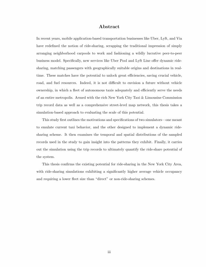
Abstract

In recent years, mobile application-based transportation businesses like Uber, Lyft, and Via

have redefined the notion of ride-sharing, scrapping the traditional impression of simply

arranging neighborhood carpools to work and fashioning a wildly lucrative peer-to-peer

business model. Specifically, new services like Uber Pool and Lyft Line offer dynamic ride-

sharing, matching passengers with geographically suitable origins and destinations in real-

time. These matches have the potential to unlock great efficiencies, saving crucial vehicle,

road, and fuel resources. Indeed, it is not difficult to envision a future without vehicle

ownership, in which a fleet of autonomous taxis adequately and efficiently serve the needs

of an entire metropolis. Armed with the rich New York City Taxi & Limousine Commission

trip record data as well as a comprehensive street-level map network, this thesis takes a

simulation-based approach to evaluating the scale of this potential.

This study first outlines the motivations and specifications of two simulators—one meant

to emulate current taxi behavior, and the other designed to implement a dynamic ride-

sharing scheme. It then examines the temporal and spatial distributions of the sampled

records used in the study to gain insight into the patterns they exhibit. Finally, it carries

out the simulation using the trip records to ultimately quantify the ride-share potential of

the system.

This thesis confirms the existing potential for ride-sharing in the New York City Area,

with ride-sharing simulations exhibiting a significantly higher average vehicle occupancy

and requiring a lower fleet size than “direct” or non-ride-sharing schemes.

iii

Acknowledgements

I could not have written this thesis without the influence of all those who have led me here.

I thank my advisor, Professor Alain Kornhauser, not only for guiding me in producingthis work, but also for serving as a great mentor for the three years that I have known him.I have always left his office thoroughly convinced of his passion for teaching, for learning,and for the University.

I thank those who have offered their support and advice at every roadblock along theway—my computationally savvy friends Edward, Edison, Brian, and Vlad, without whomI would have been quite literally unable to complete my thesis; Jinal, who ensured that nowork-induced cookie craving went unsatisfied; and Adi, who kindly made an offer to writethese acknowledgements.

I thank Derek and Neil, who have defined my experience here since day one, and all theother friends and teammates whose company I have benefited by, grown from, and reveledin since then.

I thank my sister, Nisha, whose footsteps brought me up to the gates of Princeton andhave guided me on my way out.

And, finally, I thank my parents, who have taught me love.

iv

Contents

Abstract . . . . . . . . . . . . . . . . . . . . . . . . . . . . . . . . . . . . . . . . . iiiAcknowledgements . . . . . . . . . . . . . . . . . . . . . . . . . . . . . . . . . . . ivList of Figures . . . . . . . . . . . . . . . . . . . . . . . . . . . . . . . . . . . . . vii

1 Introduction 11.1 Overview . . . . . . . . . . . . . . . . . . . . . . . . . . . . . . . . . . . . . 11.2 Motivation . . . . . . . . . . . . . . . . . . . . . . . . . . . . . . . . . . . . 31.3 Data Set . . . . . . . . . . . . . . . . . . . . . . . . . . . . . . . . . . . . . . 41.4 Existing Literature Review . . . . . . . . . . . . . . . . . . . . . . . . . . . 6

2 Objectives & Metrics 82.1 Passenger Objectives . . . . . . . . . . . . . . . . . . . . . . . . . . . . . . . 82.2 Fleet Objectives . . . . . . . . . . . . . . . . . . . . . . . . . . . . . . . . . 9

3 Simulation Design 123.1 Overview . . . . . . . . . . . . . . . . . . . . . . . . . . . . . . . . . . . . . 133.2 Taxi Creation . . . . . . . . . . . . . . . . . . . . . . . . . . . . . . . . . . . 143.3 Empty Vehicle Repositioning . . . . . . . . . . . . . . . . . . . . . . . . . . 153.4 Taxi-Passenger Hailable Area . . . . . . . . . . . . . . . . . . . . . . . . . . 173.5 Taxi Assignment . . . . . . . . . . . . . . . . . . . . . . . . . . . . . . . . . 18

3.5.1 Closest Available . . . . . . . . . . . . . . . . . . . . . . . . . . . . . 193.5.2 Passenger Time Minimization . . . . . . . . . . . . . . . . . . . . . . 223.5.3 Vehicle Mile Minimization . . . . . . . . . . . . . . . . . . . . . . . . 223.5.4 Sequential Approach; Curse of Dimensionality . . . . . . . . . . . . . 243.5.5 No Look-Ahead . . . . . . . . . . . . . . . . . . . . . . . . . . . . . . 25

3.6 Direct, or “No Ride-Share” Simulator . . . . . . . . . . . . . . . . . . . . . 26

4 Simulation Implementation 274.1 Transition Time Step . . . . . . . . . . . . . . . . . . . . . . . . . . . . . . . 274.2 Map Network . . . . . . . . . . . . . . . . . . . . . . . . . . . . . . . . . . . 28

4.2.1 Option A: Pixelation . . . . . . . . . . . . . . . . . . . . . . . . . . . 284.2.2 Option B: Street-Level Map Network . . . . . . . . . . . . . . . . . . 294.2.3 ALK Technologies Map Data Set . . . . . . . . . . . . . . . . . . . . 30

4.3 Computing the Hailable Region . . . . . . . . . . . . . . . . . . . . . . . . . 324.4 Mapping Rides to Nodes . . . . . . . . . . . . . . . . . . . . . . . . . . . . . 344.5 A Note on Runtime . . . . . . . . . . . . . . . . . . . . . . . . . . . . . . . 34

v

5 Examination of Trip Record Data 365.1 Selection of Sampled Time Window . . . . . . . . . . . . . . . . . . . . . . . 375.2 Temporal Distribution . . . . . . . . . . . . . . . . . . . . . . . . . . . . . . 385.3 Spatial Distribution . . . . . . . . . . . . . . . . . . . . . . . . . . . . . . . 41

5.3.1 Trip Volumes by Node: A Modified “80-20” Rule . . . . . . . . . . . 435.3.2 High Activity Points of Interest . . . . . . . . . . . . . . . . . . . . . 45

5.4 Walk Distances . . . . . . . . . . . . . . . . . . . . . . . . . . . . . . . . . . 48

6 Results 516.1 Vehicle Mileage and Occupancy . . . . . . . . . . . . . . . . . . . . . . . . . 516.2 Trips Shared and Fleet Sizing . . . . . . . . . . . . . . . . . . . . . . . . . . 54

6.2.1 Sharing Proportions . . . . . . . . . . . . . . . . . . . . . . . . . . . 556.2.2 Fleet Sizing . . . . . . . . . . . . . . . . . . . . . . . . . . . . . . . . 56

6.3 Summary . . . . . . . . . . . . . . . . . . . . . . . . . . . . . . . . . . . . . 63

7 Limitations, Next Steps, and Conclusion 647.1 Limitations . . . . . . . . . . . . . . . . . . . . . . . . . . . . . . . . . . . . 64

7.1.1 Limited Dataset . . . . . . . . . . . . . . . . . . . . . . . . . . . . . 647.1.2 Network Detail . . . . . . . . . . . . . . . . . . . . . . . . . . . . . . 657.1.3 Taxi Creation Dynamics . . . . . . . . . . . . . . . . . . . . . . . . . 657.1.4 Simulation Assumptions . . . . . . . . . . . . . . . . . . . . . . . . . 66

7.2 Next Steps . . . . . . . . . . . . . . . . . . . . . . . . . . . . . . . . . . . . 677.2.1 Empty Vehicle Repositioning . . . . . . . . . . . . . . . . . . . . . . 677.2.2 Passenger Convenience Tuning . . . . . . . . . . . . . . . . . . . . . 67

7.3 Closing Remarks . . . . . . . . . . . . . . . . . . . . . . . . . . . . . . . . . 68

vi

List of Figures

2.1 Demonstration of Average Vehicle Occupancy (AVO) . . . . . . . . . . . . . 10

3.1 Closest Available Assignment . . . . . . . . . . . . . . . . . . . . . . . . . . 203.2 Closest Available Assignment optimized over the system . . . . . . . . . . . 203.3 Passenger Time Minimizing Assignment . . . . . . . . . . . . . . . . . . . . 233.4 Vehicle Mile Minimization Assignment . . . . . . . . . . . . . . . . . . . . . 233.5 Considering All Possible Itineraries . . . . . . . . . . . . . . . . . . . . . . . 25

4.1 Demonstration of map path nodes . . . . . . . . . . . . . . . . . . . . . . . 304.2 Nodes composing the network of the continental United States. . . . . . . . 314.3 Simulator Network Nodes, New York City . . . . . . . . . . . . . . . . . . . 324.4 Simulator Network Nodes, Manhattan . . . . . . . . . . . . . . . . . . . . . 33

5.1 Trips By Day, 2015 . . . . . . . . . . . . . . . . . . . . . . . . . . . . . . . . 375.2 New Trips By Hour, Jan 7 - Jan 13 . . . . . . . . . . . . . . . . . . . . . . . 395.3 Trips by Day of Week . . . . . . . . . . . . . . . . . . . . . . . . . . . . . . 405.4 Visualized Taxi Trips, New York City . . . . . . . . . . . . . . . . . . . . . 415.5 Visualized Taxi Trips, Manhattan . . . . . . . . . . . . . . . . . . . . . . . . 425.6 Pick-up Heat Maps . . . . . . . . . . . . . . . . . . . . . . . . . . . . . . . . 435.7 Trip Volumes vs. Nodes—Cumulative Distribution . . . . . . . . . . . . . . 445.8 Nodes with Little Activity . . . . . . . . . . . . . . . . . . . . . . . . . . . . 455.9 Top Points of Interest . . . . . . . . . . . . . . . . . . . . . . . . . . . . . . 465.10 West Village Node Position . . . . . . . . . . . . . . . . . . . . . . . . . . . 475.11 Time Series of Trips at POIs . . . . . . . . . . . . . . . . . . . . . . . . . . 485.12 Distribution of Walk Distances to Pick-up . . . . . . . . . . . . . . . . . . . 505.13 Distribution of Walk Distances to Drop-off . . . . . . . . . . . . . . . . . . . 50

6.1 Vehicle Miles Comparison: Ride-share vs. No Ride-share . . . . . . . . . . . 526.2 AVO by Max Wait Time over Sampled Week . . . . . . . . . . . . . . . . . 546.3 Ride-sharing Percentage by Max Wait Time over Sampled Week . . . . . . 566.4 Net Taxi Inflow/Outflow per Hour at POIs . . . . . . . . . . . . . . . . . . 586.5 Cumulative Taxi Surplus/Deficit at POIs . . . . . . . . . . . . . . . . . . . 596.6 Net Taxi Sources and Sinks in Simulation Network . . . . . . . . . . . . . . 606.7 Taxis In Use—Actual Records, Direct Simulation, and Ride-share Simulation

Comparison . . . . . . . . . . . . . . . . . . . . . . . . . . . . . . . . . . . . 62

vii

Chapter 1

Introduction

1.1 Overview

At a time hailed for the rise of social networks and digital interconnectivity, we still maintain

an enormous interest in our mobility. More Americans commute and travel to work, school,

the local grocery store, and the distant outlet mall than ever before—and while the rise of

services like telecommuting, online courses, and Internet shopping may partially curb our

dependence on personal transportation, it is clear that our mobility will continue to remain,

as it has for centuries, a focal point.

On the front of physical engineering, developments have consistently redefined the stan-

dards of our means of transportation. Infrastructure, vehicle energy efficiency, and even

passenger comfort are ever-improving. Yet a truly revolutionary breakthrough—one that

goes beyond marginal improvements in personal transit and fundamentally reshapes the

paradigm of transportation—may stem from the fields of data and decision science.

Certainly, our investment to date, in both infrastructure and vehicles, has cemented

automobiles as the cheapest, most accessible means of rapid transit. Yet it is not difficult

to recognize the inefficiencies that exist. Quite simply, resources are under-shared in such a

densely populated modern economy, leaving many resources—energy, road-space, vehicles,

and time—to waste.

Technology, as it stands today, is set to disrupt the traditional vehicle-ownership model

of transportation—and indeed, in growing pockets around the globe it already has. The

1

remarkable rise of smartphones over a mere decade has rapidly boosted the feasibility of

ride-sharing. Uber, Lyft, Didi Kuaidi, Via, and other players have scrapped the traditional

notion of ride-sharing—simply arranging carpools to work in urban areas—and fashioned

a wildly lucrative peer-to-peer service business model, displacing taxi services across the

world. Equally significant, these companies have dramatically shifted attitudes about the

way we get from points A to B, replacing the “sexiness” of driving with the convenience

and agreeableness of being picked up and dropped off by a “friend” in your network or

community. The culture of driving is being redefined.

Meanwhile, rapid technological developments in a competitive field have made previously

futuristic caricatures of a self-driving car into a reality. Alphabet’s X, formerly known as

Google X, has garnered the public’s attention with its Self-Driving Car project, and may

be attributed with having lit a fire under traditional car manufacturers to undertake major

strategic initiatives to bring their own fully autonomous cars to market.

The smartphone, the sharing-economy business model, the self-driving car—individually,

these developments have been revolutionary, but together, they stand to bring about the

paradigm-shifting revolution needed to propel modern transportation into a much more

efficient future. This future is one in which cars are a resource that are not individually

owned, but rather communally used. Fleets of driverless cars—call them autonomous taxis,

or aTaxis—would be available for all to draw from.

A realization of this vision would eliminate stark inefficiencies that bog down the current

scheme. Currently, a regime of personally-owned transit serves only single individuals, as

they drive to and from their respective destinations in their own vehicles. This leads to

wasted space, wasted energy, and a wasted resource in the car itself by ignoring the potential

for ride-sharing among those with origins and destinations along a common path. A more

efficient system would not tie each car exclusively to an individual, but would instead have

firm-owned fleets that intelligently and methodically pick up passengers and drop them off

in a collectively optimal way.

Under the current taxi system, drivers act in their own self-interest, each trying to

maximize his or her own profit by serving as much demand as possible. Upon first glance,

this does not seem inconsistent with the objectives of either the passengers or the fleet—

2

more trips are made and more revenue is brought in. However, it neglects to capitalize on

the synergies that ride-sharing would offer, saving resources for the fleet and thus costs for

the passengers.

The nature of a ride-sharing system is such that there must be a central system to

guide it, matching up passengers and making assignments—it is impossible for a driver

or passenger to calculate the benefits of accommodating another trip on the go. With a

centralized fleet manager, the job of the driver shifts from that of an independent agent to

that of a chauffeur. The advent and popularization of autonomous cars, turned autonomous

taxis, could drastically drive down this cost of labor for a fleet. This, coupled with the

reduction in energy and vehicle resource costs that such a system offers, should be enough

to grow the firms and fleets that will make this vision a reality. But it all begins with

ride-sharing.

1.2 Motivation

The issue of ride-sharing has been approached in many academic settings. Over the course

of several years, students of Professor Alain Kornhauser’s course ORF 467: Transportation

Systems Analysis have sought to get an impression of what ride-sharing potential exists in

New Jersey, based on a set of trips synthesized by Talal Mufti, a former graduate student

in the department of Operations Research & Financial engineering. Previous Princeton

senior theses have grappled with the specific heuristics that may be used to conduct ride

scheduling. And numerous individuals beyond the Princeton community have in their own

right modeled the benefits that may be reaped from ride-sharing. However, the vast body

of literature lacks a key aspect that is central to any real-world implementable scheme: the

concept of dynamic ride-sharing.

On the personal or private level, dynamic ride-sharing involves creating one-time, non-

recurring trips between individuals who share geographically similar itineraries of origins

and destinations. It is distinct from traditional notions of carpooling in that there is no

long-term agreement between passengers to travel together for any time or for any purpose.

It also differs from “coincidental” carpooling in which individuals agree to share a ride on the

3

spot (for example, if two riders realize just before hailing a taxi that they share a common

destination and decide to split the fare). Dynamic ride-sharing lies somewhere in between

these two, in which there is a deliberate, short-notice matching decision process between

riders that is continuously being made throughout a trip. For example, an individual with

a car participating in the scheme may set out in the morning for work, and on the way be

notified of a nearby rider with a similar destination seeking accommodation.

This notion may be extended to apply to a taxi fleet. In this study, the term “dynamic

ride-sharing” is used to encompass a scheme in which passengers are continuously matched

together by a central fleet manager, such that each taxi capitalizes on situations in which

the sequential pick-up and drop-off of passengers proves beneficial in some capacity. The

purpose of this thesis is to contribute to this body of work by showing how the introduction

of dynamic ride-sharing to a taxi fleet can further improve the currently held views of

ride-sharing potential.

The recent implementation of “user pooling” services UberPool and Lyft Line have made

this subject of particular interest. Users who opt to take part in these services receive a

discounted fare of up to 50% if another user is picked up along the way. These private

companies recognize that the reduced fare could open up a new market segment of users,

drawing the services closer in line with cheaper public transportation options. The success

of the programs will largely depend on how successfully they can attract commuters, who

represent a significant proportion of daily rides, but are likely to place more importance on

prompt, invariable arrival time than on savings. Their present effectiveness is still unclear,

with both firms withholding their data on shared rides. However, this thesis seeks to

determine bounds on the effectiveness that these programs could achieve if widely adopted

by users.

1.3 Data Set

A complete collection of historical ride data, surely the holy grail of the transportation

science community, does not exist, nor would it be realistically feasible to generate. With

around 85% of Americans resorting to private transportation (McKenzie and Rapino, 2011),

4

the vast majority of trips taken go undocumented.

With this in mind, studies may choose to take advantage of the public transit information

that is available, understanding that it represents a mere fraction of how the population

moves itself. In urban areas with high transit system ridership, a data set provided by

authorities can be taken to be a fair representation of local mobility. However, since public

transit is much more sparsely used in suburban areas, it would be difficult to gauge how

relevant any results gleaned from rural-area data would be.

The richest data set available for a US city is provided by the New York City Taxi &

Limousine Commission (TLC) for all taxicab trips taken in the metropolitan area. With

the largest ridership participation of any American city at around 485,000 daily rides (Stiles

(2014)), the iconic yellow taxicabs are a fitting subject of study.

The TLC released record data for its taxis from January 2009 to June 2015, resorting

to transparency in its increasingly heated and public battle with ride-sharing companies,

particularly Uber. These records are very thorough, providing origin and destination co-

ordinates, pick-up and drop-off times, medallion IDs, and even fares. From this data, it

is possible to paint a very accurate picture of trips taken throughout the New York City

inner and outer boroughs. The level of detail offered is more than sufficient for conducting

transportation simulations.

Further, New York City, with its remarkably low car ownership, stands as a uniquely

ideal choice for this study. According to Sivak (2014), it is the only city in which more than

half (56%) of households do not own a vehicle, compared to 38% in Washington, D.C., the

next highest on the list, and just 9% nationwide, as of 2012. This implies a heavier focus

on public transportation—indeed, the yellow taxis are not just iconic in the city, but also

heavily used, serving hundreds of thousands of trips each day. With taxis positioned as the

preeminent mode of vehicle transportation, the TLC record set is truly the best proxy for

trips taken in the city.

Of course, in recent years, ride-sharing companies have cut into the yellow taxi mar-

ket share. A depiction of New York City rides is surely incomplete without Uber or Lyft

data, as the ride-sharing companies in the city have grown to absorb a significant propor-

tion of market share—as of June 2015, at least 11% year-over-year (Tangel)—and notably

5

surpassing taxicabs in pickups made in the outer boroughs.

Uber has released its own records as part of its legal feud with the TLC to support its

claim that it serves a vital role in serving New York commuters. The data, while more

insightful than any information previously released by the notoriously secretive company,

are far more limited than the TLC records. Each trip record contains only pick-up time and

location. Without destination information, we cannot paint a reliable picture of the trips

Uber users take, much less attempt to simulate ride-sharing. Hopefully, as these companies

continue to grow, they will offer additional transparency that will pave the way for a more

complete and insightful analysis.

With these considerations in mind, this thesis draws from the TLC’s 2015 yellow taxi

trip data for its record analysis and dynamic ride-sharing simulation.

1.4 Existing Literature Review

Ride-sharing has been investigated fairly broadly and extensively in a range of academic

settings. As mentioned previously, Professor Alain Kornhauser’s class on Transportation

Systems has over the years evaluated the ride-sharing potential in New Jersey, using a set

of synthesized data generated by Mufti. These assorted analyses serve as a sketch of the

trip dynamics, primarily used to make a judgement on the attractiveness of implementing a

ride-sharing scheme. They include investigations of cumulative trip distributions throughout

the day, estimations of the taxi fleet size necessary to serve the state, and empty vehicle

repositioning heuristics.

In their paper, Brownell and Kornhauser (2014) look into the feasibility of two potential

designs for an autonomous taxi network: the Personal Rapid Transit (PRT) model and the

Smart Para-Transit (SPT) model. A PRT model comprises several taxi stands. Riders are

grouped together into the same vehicle if they have the same origin and destination stands

(assuming there is one positioned within walking distance from any point in the serviced

region) and arrive at the origin stand within the same time window tmax. Under the SPT

model, originally proposed by Mark Gorton, riders are picked up by a vehicle at a “central

transit point.” The vehicle may then proceed to stop at one or two more central transit

6

point to pick up other passengers along the way, and it drops off passengers in a similarly

sequential fashion. Brownell and Kornhauser propose that the central transit point be

eliminated, with the taxi simply going directly to the “doorsteps” of the riders to pick them

up. The study uses Mufti & Chen’s set of synthesized data for New Jersey to conclude that

the SPT is the more economically viable implementation, both in its lower required fleet

size and its lower cost to customers.

In his senior thesis, Swoboda (2015) also used the New York TLC data, drawing records

from 2013 to investigate ride-sharing potential in New York City. Swoboda’s study involved

pixelating the city, and considering the trips taken from any pixel A to pixel B based on

the latitude-longitude coordinates provided by the trip records. He employed an enhanced

implementation of the PRT model (referred to in this paper as as an “elevator” model),

whereby all passengers participating in a trip are picked up at the same pixel—that is,

they have the same origin location—and dropped off one-by-one along the way. Passengers

would only be placed in the same vehicle if their itineraries matched certain temporal and

spatial criteria: no passenger would wait more than, say, 5 minutes, and no two passengers

would be placed in the same vehicle if their destinations were too “out of the way” of one

another.

Agatz (2010) also implemented a simulation of dynamic ride-sharing, this one in the

context of the metro-Atlanta area, which applies different optimization-based methods to

reduce vehicle miles and transportation costs. The study obtained very promising results,

especially in a city as geographically spread out as Atlanta. However, because Atlanta

lacks robust public transportation, the data used in this simulation is taken from the At-

lanta Regional Commission’s travel demand model, and is thus spatially and temporally

uncertain.

This thesis draws from the work of each of these sources. The following chapters outline

the design and implementation of a simulation built upon the solid foundation of actual trip

data provided by the New York Taxi & Limousine Commission, painting a fairly realistic

picture of the dynamic ride-sharing potential of the city.

7

Chapter 2

Objectives & Metrics

It is first key to understand the standards by which we measure a transportation system’s

effectiveness. This section discusses the relevant metrics that form the lens through which

the simulation was designed and interpreted. Intuitively, they can be understood as a

measure of how well the relevant parties (passengers and vehicles) achieve their objectives.

2.1 Passenger Objectives

The primary concern of the passenger is convenience. First and foremost, passengers want

to travel from origin to destination in as little time as possible. This translates to minimizing

the time taken from the start of their trip—marked when they first indicate demand (e.g.

“requesting” a ride in a ride-sharing app)—to their arrival.

This is naturally broken into two components: wait time (how long the passenger waits

to be picked up by a taxi) and travel time (the length of time spent in the vehicle from

pick-up to drop-off). Of course, introducing ride-sharing necessarily lengthens the total

passenger travel time. Unless passengers are matched to share rides along identical routes,

any detours for pick-up or drop-off will add time to one or multiple passengers’ journeys.

Another factor determining the passenger’s convenience is the distance he or she is re-

quired to walk before pick-up and after drop-off. In reality, we may imagine that passengers

in less densely populated regions may be required to walk to a busy intersection to find

a taxi to hail, though they are likely dropped off exactly at their desired location. In the

8

context of any study whose methodology uses discrete locations as pick-up and drop-off

points, there is the issue of determining how far a passenger must walk in order to reach

one of these points before he or she can begin a trip.

In reality, cost plays a significant role in passengers’ travel decisions. They may be willing

to accept a longer travel time at a lower price. Incorporating cost into this analysis would

require a utility function to describe passenger preferences. Because this thesis focuses more

on the operational feasibility of ridesharing (and not necessarily its economical viability),

this approach is not taken. However, a further investigation incorporating this elasticity is

warranted in order to better understand the demand dynamics at play.

2.2 Fleet Objectives

To determine the objectives of the taxis carrying out the trips, we may consider approaching

the problem from the perspective of a taxicab fleet manager.

It is first necessary to understand fixed costs—how many taxis are required to accommo-

date the entire demand of the system. This simply translates to tracking the taxi fleet size.

We may also be interested to find what percentage of fleet is being occupied at any given

time. Note that a taxi is designated as “occupied” not only if it is carrying a passenger,

but also if it is on its way to pick up a passenger that has hailed it from another location.

Continuing on to variable costs, we want to keep track of the total number of miles

that the vehicles cover, or the vehicle miles traveled. This is the figure we seek to

minimize, certainly from a business perspective to help support claims of a ride-sharing

system’s viability, but also from a municipal perspective (a lower total distance covered

likely means less traffic, if demand is held constant) and a “green” perspective (with fewer

resources dedicated to fueling vehicles).

From an academic perspective, to truly gauge the effectiveness of ride-sharing, we are

particularly interested in the average vehicle occupancy (AVO) of the system. Intu-

itively, this metric captures the extent to which ride-sharing is being used. The higher the

AVO, the more effective the ride-share policy is at matching passengers and the more miles

are being saved. But how exactly should it be calculated?

9

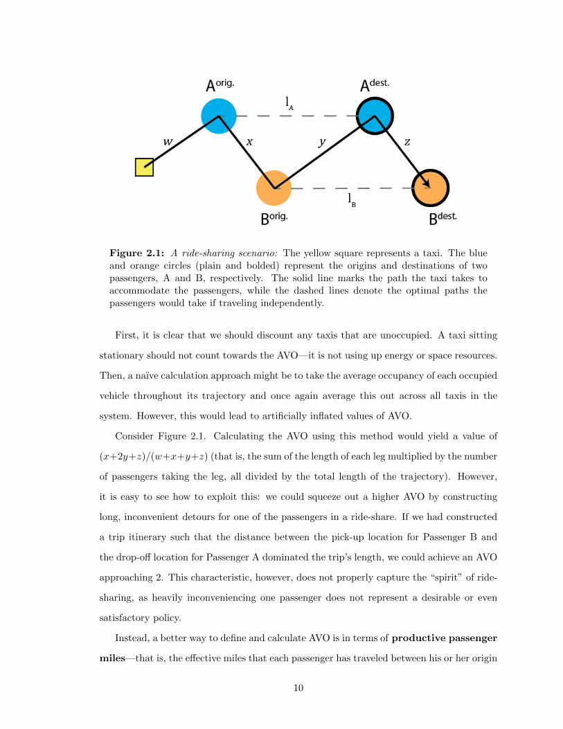
Figure 2.1: A ride-sharing scenario: The yellow square represents a taxi. The blueand orange circles (plain and bolded) represent the origins and destinations of twopassengers, A and B, respectively. The solid line marks the path the taxi takes toaccommodate the passengers, while the dashed lines denote the optimal paths thepassengers would take if traveling independently.

First, it is clear that we should discount any taxis that are unoccupied. A taxi sitting

stationary should not count towards the AVO—it is not using up energy or space resources.

Then, a naıve calculation approach might be to take the average occupancy of each occupied

vehicle throughout its trajectory and once again average this out across all taxis in the

system. However, this would lead to artificially inflated values of AVO.

Consider Figure 2.1. Calculating the AVO using this method would yield a value of

(x+2y+z)/(w+x+y+z) (that is, the sum of the length of each leg multiplied by the number

of passengers taking the leg, all divided by the total length of the trajectory). However,

it is easy to see how to exploit this: we could squeeze out a higher AVO by constructing

long, inconvenient detours for one of the passengers in a ride-share. If we had constructed

a trip itinerary such that the distance between the pick-up location for Passenger B and

the drop-off location for Passenger A dominated the trip’s length, we could achieve an AVO

approaching 2. This characteristic, however, does not properly capture the “spirit” of ride-

sharing, as heavily inconveniencing one passenger does not represent a desirable or even

satisfactory policy.

Instead, a better way to define and calculate AVO is in terms of productive passenger

miles—that is, the effective miles that each passenger has traveled between his or her origin

10

and destination. In Figure 2.1, for example, the productive passenger miles of the trip would

be equal to lA + lB. This way, rather than rewarding a policy that misguidedly tries to

maximize the length of the leg with the most passengers, the metric benefits policies that

make minimal detours. The AVO, then, is defined as:

AV O =total productive miles

total vehicle miles

Or, in the example of Figure 2.1:

AV O =lA + lB

w + x+ y + z

Indeed, what makes AVO such a good metric for measuring the effectiveness of ride-

sharing is the fact that it captures both of the relevant considerations from the fleet man-

ager’s perspective—fleet size and vehicle miles traveled. A policy that simply seeks to

minimize the fleet size might heavily inconvenience passengers—using fewer cars may mean

long detours that in fact cost more miles than if multiple taxis were used. Meanwhile, a

policy that aims to minimize vehicle miles traveled might use too many taxis. For example,

the two rides in Figure 2.1 could be addressed with two separate taxis, each starting at the

respective passenger’s location and going straight to the destination. However, this unnec-

essarily uses two cars when just one would serve the system well. AVO strikes a balance

between these two scenarios: it uses as few cars as makes sense to serve the system.

As outlined in the introduction, this thesis has its basis in the fleet model, in which

a central manager makes passenger assignments to its taxis. It is reasonable to assume

that such a model would be driven towards optimizing the vehicle objectives, as outlined

in this chapter. Certainly, the passenger objectives must be taken into account—the fleet

model could not be brought into existence if it did not properly address the needs of its

users. However, we can think of the system as an problem in which we optimize the fleet’s

objective, subject to the passengers’ constraints. For this reason, vehicle miles, AVO, and

fleet size will be the key metrics driving the study, and will form the basis upon which the

ride-sharing potential of the system is judged.

11

Chapter 3

Simulation Design

As described in the Introduction, the primary objective of this thesis is to investigate the

ride-share potential of trips in the city when a dynamic ride-sharing scheme is adopted.

In order to implement dynamic ride-sharing, it was necessary to build a simulator that is

altogether distinct from those that have been used for trip analyses thus far.

Swoboda took the approach of the “elevator” model, whereby all passengers share the

same origin. His promising results should serve as a lower bound for the ride-sharing poten-

tial of New York City. A more realistic model (like the scheme implemented in Uber Pool

or Lyft Line) would allow for interspersed pick-up and drop-off, presumably improving the

vehicle occupancy rate of each vehicle, as vehicles would not need to complete in-progress

trips before beginning on a new trip. The study by Brownell & Kornhauser addressed this

issue with the SPT model. However, this analysis, like Swoboda’s, involved the pixelation

of the travel region and the use of a heuristic to calculate the distance and circuity between

pixels.

The simulator built in this study seeks to address these concerns. Namely, the major

enhancements it offers are its implementation of continuous hailing and its use of a

realistic street-level map network. This chapter focuses on how the simulation conducts its

continuous hailing scheme. An in-depth discussion of the strengths of using a map network

is included in Chapter 4.

12

3.1 Overview

Broadly described, the simulator chronologically carries out the trips listed in the New York

TLC data set, matching passengers with taxis throughout the system as it steps through

time. The simulation could, in theory, be conducted over an arbitrarily long trip record time

frame, subject only to constraints on data (the periods for which trip records are available)

and time (the computational burden of completing the simulation). Given that the New

York TLC data spans a 6 1/2 year period from 2009 to 2015, it would be a fair challenge

to run the simulation through the entire record set.

The simulator limits the number of passengers (or unique trips) that can simultaneously

share a taxi to 2. The true reason for this lies in computational efficiency. As explained

in Section 3.5, the algorithm for matching rides suffers the curse of dimensionality and

exhibits factorial time complexity—increasing the number of passengers that each car could

accommodate would render the simulator far too slow to produce any worthwhile results.

Services like Uber Pool and Lyft Line, too, cap ride-shares at 2 unique trips per vehicle

at a time. So while this decision costs the simulator some generality from an academic

standpoint, it does not impose any significant reservations on its results from a practical

standpoint.

At each discrete time step, the simulator checks the trip record set to see if any users

had “hailed” a cab. This would be indicated by the trip start time in the record set. For

each new ride request that is created, the simulator searches for any taxis “in the area” of

the trip’s origin that are available to carry out the trip. This “hailable area,” naturally, is

dependent on how long we are willing to make the passenger wait and how quickly a hailed

taxi could arrive to accommodate the trip (see Section 3.4 for further discussion). Further,

whether a taxi in the area is able to carry out the trip depends on whether it is already

transporting a passenger—and if so, whether the detour needed to accommodate the new

passenger would overburdensome to either party.

If no taxis in the hailable region are well-able to accommodate the passenger, a new taxi

is spawned after the maximum allowable wait time tmax at the user’s location in order to

fulfill the trip. This value was modified for each round of the simulation, set to 1 minute, 3

13

minutes, 5 minutes, and 10 minutes. An alternative approach may have a tmax that varies

as a function of time—passengers may be expected to wait longer for a taxi late at night

than in the early afternoon.

If multiple taxis in the hailable region are available, the simulator assigns the “best one”

to the requesting rider. Naturally, the determination of which of the options is best depends

on the metric used to rank them. This issue is considered in Section 3.5.

The simulator is also responsible for advancing taxis at each time step from one point

to the next and for dropping off passengers when necessary.

3.2 Taxi Creation

An important design decision early on concerned the “initial state” of the system—determining

how many taxis would be included and how they would be placed at the outset of the sim-

ulation. A few approaches were considered.

One approach would be to determine how many unique taxis were used to accommodate

all the trips in the TLC trip data file (a calculation made possible by the inclusion of a

medallion ID for each trip record), and then distribute each of these taxis at the position

of their first trip in the records.

Another approach that was considered was using the trip records to determine the

demand over time at each discrete location in the system and setting the fleet size equal to

the peak total demand ever observed across any such positions. The initial distribution of

taxis, then, could be made according to the initial demand seen at each of these discrete

locations.

However, the simulator adopts a third approach that appears more organic, albeit less

natural: it initializes the system with zero taxis and creates them only as needed. Whenever

a passenger cannot not find a taxi in the area, a new taxi is spawned for him or her, drawn

from a “super-source” of taxis. This means that at the outset, taxis are only rarely hailed

from the surrounding region, and trip demand emerging around the city forces the rapid

creation of new taxis. As the system approaches a functional fleet size, we could imagine

that taxis would rarely need to be spawned—it would be more likely (given the higher

14

volume of taxis) that there would be one available in the area. That is, the system would

become self-preserving.

Of course, the value of this design decision is limited without an anticipatory empty

vehicle repositioning plan (see Section 3.3). We would expect that taxis would seldom end

up in less densely populated parts of the city (say, in Far Rockaway, Queens), as few trips

terminate there. Thus, when new trips spawn in these locations, they would likely force

new taxis to be created. Further, when a taxi does end up in an area of lower demand, it

is less likely that a trip will soon arise near its location to “draw it out,” returning it to

a high demand location once again. From the outset of the study, it was understood that

these concerns about the taxi creation strategy would hamper the simulation’s ability to

properly estimate fleet size. The extent of their effect is described and discussed in Chapter

6.

3.3 Empty Vehicle Repositioning

Empty vehicle positioning—the movement of taxis containing no passengers, usually in

anticipation of demand at another location—would be key to fully characterize the behavior

of a taxi fleet. Indeed, taxis do not simply sit around after completing their trips, waiting

for new passengers to arrive at the location of their last drop-off. Rather, they may move

to a more populous area where they anticipate more demand. For example, a taxi that

completes a trip in South Jamaica may head to JFK, a high demand location, to catch a

fare from incoming travelers.

In reality, these decisions are left up to each individual taxi driver—they are not made

systematically. This is what makes simulating empty vehicle repositioning so difficult. A few

models and heuristics were considered, but due to the complexity of their implementation

and computation, this simulation does not adopt any such policy. Nevertheless, this section

includes a discussion of these models, with the hope that it may assist in any future iterations

of this study.

All models would involve properly modeling trip demand, or the “arrivals” of trips at

each discrete location in the system. We could use TLC trip record data to tune a non-

15

homogeneous Poisson process with a parameter λ(t) that is reflective of historical demand.

With this, at each time step we could determine the expected demand that may arise at

each discrete location in the system.

Much of the existing literature has taken a theoretical model-based approach. The

majority of models involve minimizing over a cost function, with costs corresponding to

passenger wait times and taxi travel distance. Song and Earl (2008) propose such a model in

their paper “Optimal Empty Vehicle Repositioning and Fleet-sizing for Two-depot Service

Systems,” with additional costs for vehicle maintenance and “leasing” (analogous to the

creation of new taxis in our system). However, their solution does not extend well to the

system considered in this thesis, which is of a much greater size. In his senior thesis “Truly

Empty Vehicle Repositioning and Fleet-Sizing,” Douglas (2015) addresses this issue by

proposing a model that accommodates a system of any size. However, it does not account

for the complications introduced by dynamic ride-sharing

Introducing the continuous hailing aspect of dynamic ride-sharing adds significant com-

plexity to the theoretical models proposed. A look-ahead policy, as is used in Douglas’s

study, would be rendered ineffective—each time a ride-sharing opportunity is created, the

state of the system diverges greatly. Douglas’s model rests on the assumption of deter-

ministic travel time in order to compute exactly when a taxi will arrive at a destination

and be available for use. And rightly so—without continuous hailing the taxi’s itinerary is

written in stone the moment it departs (or within a range of error if traffic is considered).

However, with continuous hailing, each taxi’s path becomes stochastic, as during its route it

may be diverted to pick up a passenger along the way, taking a detour and almost certainly

postponing its original destination arrival time. Thus, no matter how well the demand at

each discrete location is modeled, it would be difficult to determine the location and state

of taxis and passengers more than a few minutes ahead.

Rather than seeking to actually optimize vehicle repositioning, however, an intuitive

heuristic could be adopted. The estimates of trip arrivals could be used to look ahead to

what the demand distribution in the system may be, say one hour from now—that too

without “cheating” since our model for demand is trained on historical data (not including

the “testing” trip file used for conducting the simulation), and is only an estimate of what we

16

expect throughout the day. Based on these estimates, we could broadly relocate taxis from

areas of lower expected demand to areas of higher expected demand on a vehicle-by-vehicle

basis. This is the key difference: while the theoretical models seek to find a system-wide

optimum, this relocation “policy” would be made based on a rough notion of self-interest.

This seems intuitive—around 5 PM we can imagine taxi drivers consciously relocating to

office-dense regions of Manhattan, like downtown and midtown, hoping to pick up fares

for passengers leaving work and heading home. Rather than being assigned to a specific

location, they gravitate to where they expect to find a fair.

An implementation of this policy could take several forms. For example, we can imagine

a gravity model of attraction where the “mass” of each discrete location at each time step

is proportional to the expected demand at that time, and the strength of “attraction” for

taxis is inversely proportional to their distance from that location, squared. Alternatively,

we could take a gradient-based approach, where a taxi relocates to an adjacent location if

the expected demand there is higher than at its present location.

As noted, this simulation does not include a repositioning model or heuristic. However,

empty vehicle repositioning is a key characteristic of taxi behavior, and an examination of

these heuristics would certainly warrant its own distinct investigation.

3.4 Taxi-Passenger Hailable Area

A key decision made when building the simulator was determining how “close” a taxi must

be to a passenger in order to be considered for pick-up. This naturally reduces to the

question, what is a reasonable amount of time for the passenger to wait? In a 2014 New

York City Council hearing, a regional manager for Uber revealed that the average wait

time for Uber pick-ups is under five minutes—even in the outer boroughs (Mosendz and

Sender). With ride-share services growing both in fleet size (more drivers available) and in

ridership (more users requesting), it is unclear whether this average would be high or low in

today’s context. As mentioned in the Overview, the maximum wait time parameter, tmax,

was modified for each run of the simulation, set to 1, 3, 5, and 10 minutes.

Given the taxi’s travel speed, we can determine how far away it can be and still reach

17

the passenger within a time of tmax. Thus, for each imposed maximum wait time, we can

determine the implied distance threshold, dmax.

In a post on his popular NYC data blog I Quant NY, data scientist Ben Wellington

(2014) used the same TLC trip data to estimate the average taxi speed in New York City

at different times during the day. Drawing from his results, the simulation uses the speed

v = 11.5 miles per hour, which Wellington found to be the roughly constant average speed

between 7am and 8pm.

Thus, for each passenger, the simulator searches for any taxis located within a “radius”

of dmax = v× tmax. This area does not exactly define a circle, of course, especially in a city

with a grid-like layout and many one-way streets. Rather, the term “radius” is used here

to define the boundaries of an area within which the passenger can be reached in at most

dmax miles of road traveling distance.

Note that the maximum wait time is the upper threshold on searching for a vehicle

match. It does not include the amount of time that it takes for the taxi, once hailed, to

arrive at the passenger’s location. This means that in the worst case under a tmax = 5

minute scheme, the passenger could actually wait 10 minutes, if a match is made after

exactly 5 minutes of searching and the taxi that is chosen is exactly 5 minutes away. Thus

tmax may be better described as a maximum search time. As described previously, after

searching for the maximum allotted time, the passenger is simply granted a “new” taxi

spawned at his or her location to carry out the trip.

3.5 Taxi Assignment

The simulator overview suggested that when searching for ride-share opportunities, it is

the simulator’s task to determine and assign the “best” choice of match between taxi and

passenger. Naturally, this raises the question of how these choices should be compared. To

answer this, we must enumerate the parties whose interests are relevant in the making of

the decision and recognize their objectives.

First, there is the roadside passenger who is hailing the taxi to be picked up. This

passenger’s priority is arriving at his or her destination as soon as possible.

18

In addition, in a ride-sharing system, there may be other passengers (specifically under

the constraints of our system, up to one other passenger) who are also being accommodated

by the same taxi—whether they are already in the taxi or have already been assigned are

awaiting pick-up. Their objective, too, is to arrive at their destination(s) as soon as possible.

Of course, in reality, this is not a passenger’s only consideration—cost and comfort come

into play, as well. The passenger may be willing to take a longer route to avoid tolls at a

bridge, for example. Or, relevant to ride-sharing, a passenger may value his or her privacy

during the trip. However, for the purpose of this investigation, whose goal is to determine

ride-sharing viability, we reduce their priorities to simple service duration minimization.

Finally, there is the taxi driver. In this study, we do not enable drivers to make their

own decisions. Rather, taxi behavior is dictated by some “master” decision-making unit. In

the simulator, this unit would be the set of rules methodically assigning taxis to passengers.

However, this is not too unrealistic in the modern landscape of transportation. Uber and

Lyft drivers are not responsible for finding their own fares—rather, they are matched with

app users by a central server. Even New York taxis have introduced a hailing app. Indeed,

this extends well to the aTaxi vision, where the fleet would be controlled by a central system.

For the fleet, then, the objective is a combination of minimizing the total miles traveled

by all taxis in the system and minimizing the size of the fleet necessary to serve all de-

mand. In Chapter 2, we recognized that maximizing average vehicle occupancy is the best

combination of this dual objective.

Certainly, the objectives of passenger and fleet are often at odds. Without fares as a

factor, passengers would never prefer to share a ride, as doing so could only inconvenience

them. Meanwhile, the fleet actively seeks to create ride-sharing opportunities, as therein

lies the potential to save mileage and reduce fleet size. With this in mind, this section

proposes three frameworks for comparing assignment opportunities.

3.5.1 Closest Available

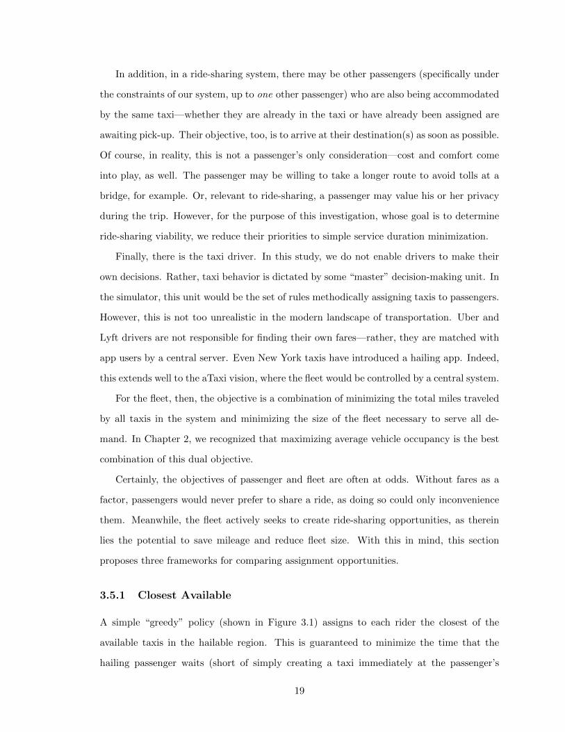
A simple “greedy” policy (shown in Figure 3.1) assigns to each rider the closest of the

available taxis in the hailable region. This is guaranteed to minimize the time that the

hailing passenger waits (short of simply creating a taxi immediately at the passenger’s

19

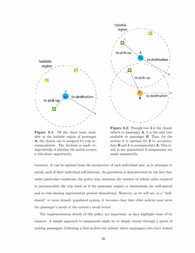
Figure 3.1: Of the three taxis avail-able in the hailable region of passengerA, the closest one is assigned for trip ac-commodation. The decision is made in-dependently of whether the match createsa ride-share opportunity.

Figure 3.2: Though taxi 2 is the closestvehicle to passenger A, it is the only taxiavailable to passenger B. Thus, for thesystem it is optimal for 2 to accommo-date B and 1 to accommodate A. This re-sult is not guaranteed if assignments aremade sequentially.

location). It can be optimal from the perspective of each individual user, as it attempts to

satisfy each of their individual self-interests. Its greediness is demonstrated by the fact that

under particular conditions, the policy may minimize the number of vehicle miles required

to accommodate the trip (such as if the passenger origins or destinations are well-spaced

and no ride-sharing opportunities present themselves). However, as we will see, in a “well-

shared” or more densely populated system, it becomes clear that other policies may serve

the passenger’s needs or the system’s needs better.

The implementation details of this policy are important, as they highlight some of its

nuances. A simple approach to assignment might be to simply iterate through a queue of

waiting passengers (following a first-in-first-out scheme where passengers who have waited

20

the longest are assigned first) and sequentially assign to each the closest taxi. This seems

both fair and realistic.

However, this could bring up a scenario as shown in Figure 3.2, where the order by which

we iterate through the list of passengers could drastically affect the assignment end-result.

In this example, we see that without considering the entire system as a whole, we run the

risk of creating a system with sub-optimal assignment. An alternative approach would be

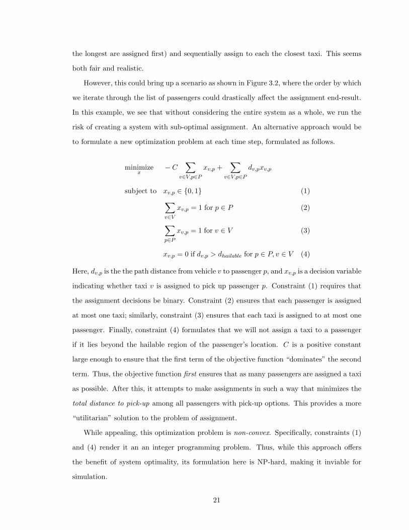
to formulate a new optimization problem at each time step, formulated as follows.

minimizex

− C∑

v∈V,p∈Pxv,p +

∑v∈V,p∈P

dv,pxv,p

subject to xv,p ∈ {0, 1} (1)∑v∈V

xv,p = 1 for p ∈ P (2)

∑p∈P

xv,p = 1 for v ∈ V (3)

xv,p = 0 if dv,p > dhailable for p ∈ P, v ∈ V (4)

Here, dv,p is the the path distance from vehicle v to passenger p, and xv,p is a decision variable

indicating whether taxi v is assigned to pick up passenger p. Constraint (1) requires that

the assignment decisions be binary. Constraint (2) ensures that each passenger is assigned

at most one taxi; similarly, constraint (3) ensures that each taxi is assigned to at most one

passenger. Finally, constraint (4) formulates that we will not assign a taxi to a passenger

if it lies beyond the hailable region of the passenger’s location. C is a positive constant

large enough to ensure that the first term of the objective function “dominates” the second

term. Thus, the objective function first ensures that as many passengers are assigned a taxi

as possible. After this, it attempts to make assignments in such a way that minimizes the

total distance to pick-up among all passengers with pick-up options. This provides a more

“utilitarian” solution to the problem of assignment.

While appealing, this optimization problem is non-convex. Specifically, constraints (1)

and (4) render it an an integer programming problem. Thus, while this approach offers

the benefit of system optimality, its formulation here is NP-hard, making it inviable for

simulation.

21

3.5.2 Passenger Time Minimization

The “Closest Available” policy is poised to prioritize the needs of the waiting passengers. It

certainly makes sense for a non-ride-sharing system: with the origin and destination points

of a single passenger fixed, the policy seeks to minimize the only variable with a degree of

freedom: the distance to pick-up.

However, the policy would be quite naıve for a ride-sharing scheme. First, the objective

function solely considers the preferences of the hailing passenger, without consideration for a

passenger already in tow (if a taxi already containing a passenger is selected for assignment).

More strikingly, however, is the fact that remarkably sub-optimal ride-share matches could

arise. If a taxi containing a passenger is assigned to pick-up a second passenger simply

because it is nearby, it could make a significant detour to drop off either of the passengers.

That is, the Closest Available policy does not take into account the itinerary of taxis beyond

pick-up.

To address this issue, we might choose to implement a policy that weighs the needs of

both passengers evenly. Such a policy may seek to minimize the total time burden placed on

all passengers whose interests are involved in the assignment decision. The Closest Available

policy would minimize the total wait time of all hailing passengers. But Passenger Time

Minimization minimizes the total trip time (from the time the assignment takes place to the

time the trip is completed) of both passengers. Thus, this policy would avoid long detours

for either passenger involved. However, this would often come at the cost of forfeiting

ride-share opportunities as demonstrated in Figure 3.3—if a sufficient number of taxis are

available and appropriately positioned to service all waiting passengers, the time-minimizing

assignment would grant each passenger their own taxi, when in fact making a ride-share

match would only create a minor detour.

3.5.3 Vehicle Mile Minimization

Both the Closest Available and Passenger Time Minimization policies formulate optimiza-

tion decisions from the perspective of passengers. However, it is more realistic to optimize

assignment from the perspective of the fleet manager. After all, the assignment decision

22

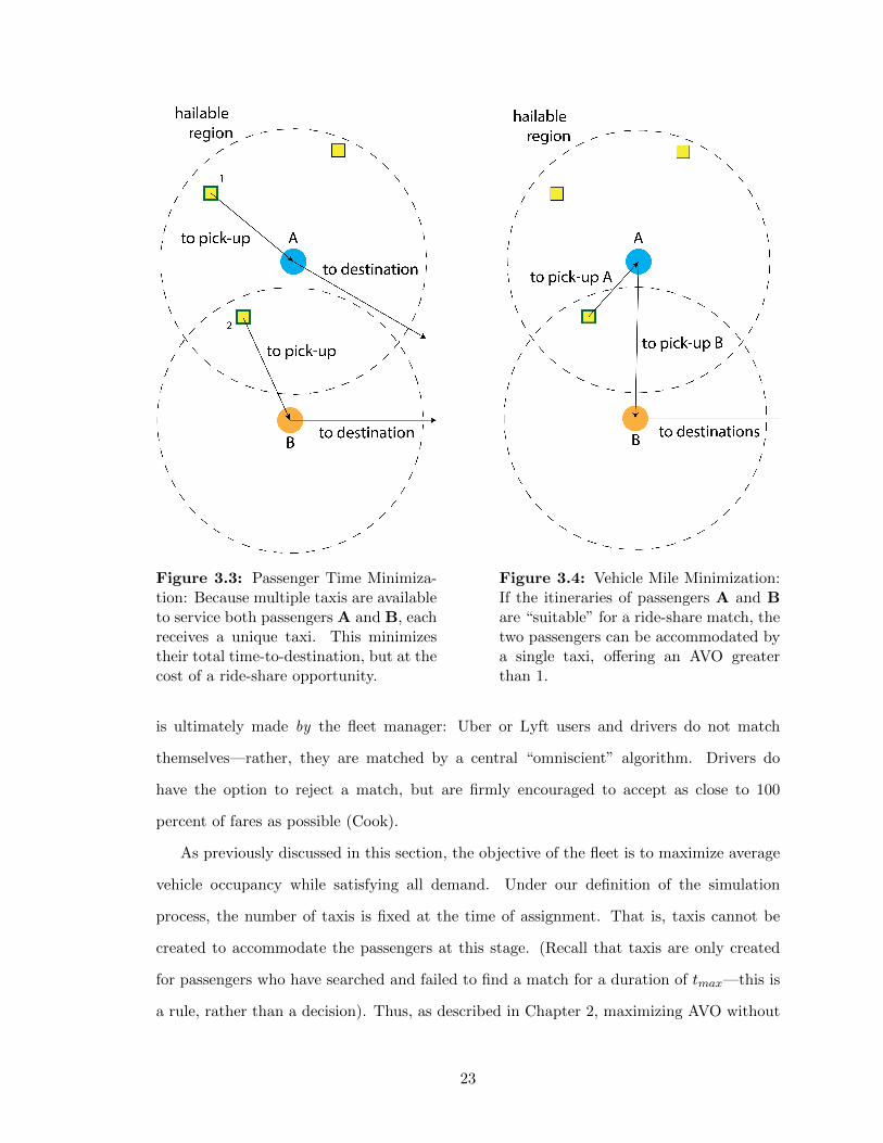
Figure 3.3: Passenger Time Minimiza-tion: Because multiple taxis are availableto service both passengers A and B, eachreceives a unique taxi. This minimizestheir total time-to-destination, but at thecost of a ride-share opportunity.

Figure 3.4: Vehicle Mile Minimization:If the itineraries of passengers A and Bare “suitable” for a ride-share match, thetwo passengers can be accommodated bya single taxi, offering an AVO greaterthan 1.

is ultimately made by the fleet manager: Uber or Lyft users and drivers do not match

themselves—rather, they are matched by a central “omniscient” algorithm. Drivers do

have the option to reject a match, but are firmly encouraged to accept as close to 100

percent of fares as possible (Cook).

As previously discussed in this section, the objective of the fleet is to maximize average

vehicle occupancy while satisfying all demand. Under our definition of the simulation

process, the number of taxis is fixed at the time of assignment. That is, taxis cannot be

created to accommodate the passengers at this stage. (Recall that taxis are only created

for passengers who have searched and failed to find a match for a duration of tmax—this is

a rule, rather than a decision). Thus, as described in Chapter 2, maximizing AVO without

23

the ability to change fleet size translates to minimizing the total vehicle miles resulting from

matches made during this time step. This will result in a ride-share match, shown in Figure

3.4, if the itineraries of the two passengers are “suitable”—that is, as long as the number

of vehicle miles resulting from the match is less than the total vehicle miles accrued if each

passenger were serviced individually (as in Figure 3.3). This simple rule presses ride-sharing

while ensuring that neither passenger is subject to a significant detour.

3.5.4 Sequential Approach; Curse of Dimensionality

Vehicle Mile Minimization is the policy ultimately used in the simulator, both for its resem-

blance to real-world ride-sharing schemes and for its natural maximization, the metric we

are most focused on. Like the optimization problem posed for the Closest Available policy,

a similar formulation for Vehicle Mile Minimization would also be non-convex (primarily

due to the constraint that assignment of taxis to passengers must be one-to-one). Thus,

the simulation’s implementation of this policy is sequential—it iterates through a list of

as-of-yet unattended passengers, assigning to each the “best” match given what is known

at that state of the simulation. The order by which we iterate through this list certainly

has the potential to affect the optimality of the assignment. However, given the scale of the

simulation, this loss of optimality was considered minor.

The policy must dynamically determine which of the taxis available to each unattended

passenger would be optimal for pickup through an exhaustive calculation. For each avail-

able taxi, a hypothetical trajectory must be created, whereby the taxi accommodates the

passenger by adding his pick-up and drop-off points to its itinerary. The taxi for which this

hypothetical accommodation would add the fewest additional vehicle miles is assigned to

pick up the passenger.

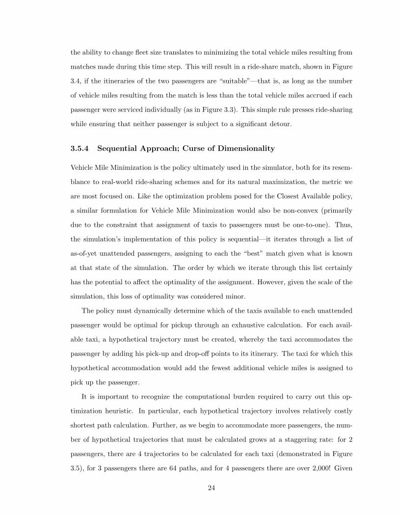
It is important to recognize the computational burden required to carry out this op-

timization heuristic. In particular, each hypothetical trajectory involves relatively costly

shortest path calculation. Further, as we begin to accommodate more passengers, the num-

ber of hypothetical trajectories that must be calculated grows at a staggering rate: for 2

passengers, there are 4 trajectories to be calculated for each taxi (demonstrated in Figure

3.5), for 3 passengers there are 64 paths, and for 4 passengers there are over 2,000! Given

24

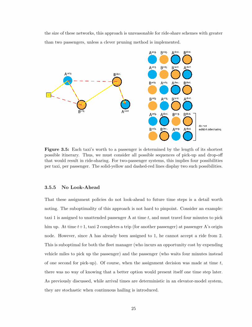
the size of these networks, this approach is unreasonable for ride-share schemes with greater

than two passengers, unless a clever pruning method is implemented.

Figure 3.5: Each taxi’s worth to a passenger is determined by the length of its shortestpossible itinerary. Thus, we must consider all possible sequences of pick-up and drop-offthat would result in ride-sharing. For two-passenger systems, this implies four possibilitiesper taxi, per passenger. The solid-yellow and dashed-red lines display two such possibilities.

3.5.5 No Look-Ahead

That these assignment policies do not look-ahead to future time steps is a detail worth

noting. The suboptimality of this approach is not hard to pinpoint. Consider an example:

taxi 1 is assigned to unattended passenger A at time t, and must travel four minutes to pick

him up. At time t+1, taxi 2 completes a trip (for another passenger) at passenger A’s origin

node. However, since A has already been assigned to 1, he cannot accept a ride from 2.

This is suboptimal for both the fleet manager (who incurs an opportunity cost by expending

vehicle miles to pick up the passenger) and the passenger (who waits four minutes instead

of one second for pick-up). Of course, when the assignment decision was made at time t,

there was no way of knowing that a better option would present itself one time step later.

As previously discussed, while arrival times are deterministic in an elevator-model system,

they are stochastic when continuous hailing is introduced.

25

We could characterize the policies described in this section as “eager” or “anxious.” At

each time step t, they seek to make assignments for all passengers as soon as possible—that

is, assignments for time t are made at time t. The benefits from a computational perspective

are clear, as there is no need to create, update, and reference probability distributions of taxi

arrival times. But we can also justify our approach from a risk-management perspective.

The assumption underlying this heuristic is that it is better to make a decision now than to

wait for potentially better options to present themselves later. Indeed, since our foremost

goal is to accommodate all demand, it is logical that we first ensure that all passengers

are accommodated, and only after that concern ourselves with the optimality of these

assignments.

3.6 Direct, or “No Ride-Share” Simulator

In judging the results of the dynamic ride-sharing simulator, making a comparison to the

actual TLC trip record set is not sufficient. When calculating vehicle miles traveled, it

would be unfair to sum the distances of the trips provided in the TLC records, when the

paths taken to fulfill the trips may have been different from the shortest path calculated

and used in the simulator. Further, because it lacks an empty vehicle repositioning policy,

it is expected that the simulation would yield a fleet size far greater than that of the actual

records.

Thus, to create a benchmark off which to base ride-share results, it was necessary to also

build a simulator that does not implement dynamic ride-sharing. This simpler simulation,

referred to in this thesis as the “no ride-share” or “direct” implementation, simply allows

each taxi a maximum of one passenger at a time. Thus, the taxi spawning, advancement, and

drop-off processes are conducted identically to the ride-share simulator as described above.

However, for taxi assignment, only the distance between each taxi and the passenger’s origin

is considered in determining the best available taxi (the Closest Available policy).

With this simplified scheme, we will be able to make a more appropriate judgement of

the effectiveness of the ride-sharing scheme, both in terms of the vehicle miles it saves and

the reduced fleet size it allows.

26

Chapter 4

Simulation Implementation

Chapter 3 outlined the principles guiding the simulator. This chapter offers a closer look

at the “grittier” details that went into the actual building of the simulator. Specifically, it

outlines the decision to employ a map network on which to run the simulation, then details

the consequences this choice had on implementing the design described in the preceding

chapter. A thorough understanding of the simulation’s mechanics here can provide better

insight into the robustness and limitations of its results.

4.1 Transition Time Step

As referenced throughout the design description, the simulation “ticks” at each discrete

time step—new rides are created, vehicle assignments are made, passengers are picked up

and dropped off, and taxis are advanced at each interval.

An important parameter in the simulation, then, is the size of this time step, ∆t. There

is an apparent trade-off between speed and precision. Naturally, a smaller ∆t ensures higher

definition—trips are recognized by the simulator closer to the time they are created and

taxis are displaced small distances, sharpening figures like passenger travel times and vehicle

miles traveled. A larger ∆t, however, is more appealing from a computational perspective—

having fewer iterations would allow the simulation to complete in a shorter time.

Because the trip record data provided by the TLC has second-level precision, and to

ensure the metrics observed would be as sharp as possible, ∆t was set to 1 second. However,

27

this imposed a significant trade-off, as due to run-time constraints the study could use only

one week’s worth of records for the simulation. The trip records used is characterized in

Chapter 5.

4.2 Map Network

Two options were considered for constructing the map network on which the simulation

would run: a pixelated network and a street-level map network. Both are described below

in order to better understand the merits of each.

4.2.1 Option A: Pixelation

A crude but appealing option for constructing the map is pixelating the travel region.

Previous studies, such as Brownell and Kornhauser (2014), Swoboda (2015), and Douglas

(2015) have relied on pixelation for assorted analyses.

For urban areas, this pixelation could be granular, so that each pixel roughly corresponds

to a city block. For suburban areas, the pixels could be larger—for example, 0.1 by 0.1

mile squares. Either square or hexagon pixels could be used—a trade-off of flexibility and

convenience. A square-based grid would be much easier to generate and maintain, but

limits vehicle movement to four directions, providing the “Manhattan” distance between

two pixels. A hexagon-based grid would be more difficult to generate but would allow for

diagonal travel, giving a better idea of travel distances and times in suburban areas that do

not exhibit a grid-like structure.

Under this method, at any given time, a taxi would be located in one of the pixels,

allowing the simulator to keep track of each vehicle’s exact position. At each time step (or

after several time steps, depending on the pixel size), the taxi would move to an adjacent

pixel. The simulator would continuously update vehicle trajectories as new ride requests

appear.

This approach is appealing for taxi assignment, the most computationally intensive stage

of each time step. Transitioning from t to t+1 would simply involve sweeping through each

pixel and “looking” at the cells immediately surrounding it. It would also simplify post-

28

simulation data analyses. We could easily approximate areas of high activity by selecting

pixels with the most pick-ups, drop-offs, and taxi assignments.

The pixelation method would serve as a fair heuristic for modeling ride-sharing in New

York City, which in most of Manhattan and much of Brooklyn exhibits a characteristic

gridded layout. However, it would not appropriately capture travel through the outer

boroughs (Brooklyn, the Bronx, Staten Island, and Queens) or even in southern parts of

Manhattan where the streets break from their neat layout. Modeling travel across bridges

would also pose an issue, as a naıve model would unrealistically have traffic crossing over

any point of the East River (say, from Brooklyn to Manhattan). Further, it would neglect

to address traffic patterns (one-way streets, no-turn streets, etc.) that are key to New York

City travel, and must certainly have a collective impact on ride-share feasibility. The real

path between a passenger’s origin and destination is likely circuitous, not a simple direct

path across square or hexagonal pixels.

While the pixelation method would be relatively easy to work with and would provide

a broad sense of the ride-sharing potential of the studied regions, the results drawn from it

would come with reservations.

4.2.2 Option B: Street-Level Map Network

A truly comprehensive simulator would make use of map data in order to construct trips

along routes. The term “street-level map network” is used here to refer to an extensive

set of nodes and arcs connecting one location of interest with another. This notion is

demonstrated in Figure 4.1. The weight of each arc is equal to the travel distance between

the two nodes it connects.

Figure 4.1 serves as an example of the preferred level of detail for conducting the simu-

lation. By maintaining a highly defined network of nodes and arcs, the simulator could keep

track of the exact coordinate (effectively) of each vehicle at every point in time. Intersection

nodes are essential in order to guarantee shortest-path calculations are direct. Path-defining

nodes would allow a greater degree of precision when setting origins, destinations, and the

positions of taxis. For this reason, they are favorable but not necessary; indeed, in New York

City, where intersections are already relatively closely spaced, the benefit of path-defining

29

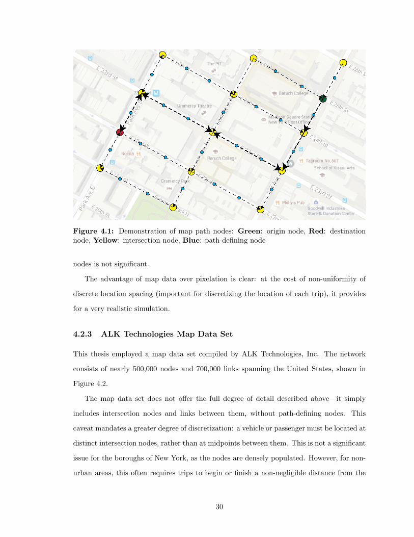
Figure 4.1: Demonstration of map path nodes: Green: origin node, Red: destinationnode, Yellow: intersection node, Blue: path-defining node

nodes is not significant.

The advantage of map data over pixelation is clear: at the cost of non-uniformity of

discrete location spacing (important for discretizing the location of each trip), it provides

for a very realistic simulation.

4.2.3 ALK Technologies Map Data Set

This thesis employed a map data set compiled by ALK Technologies, Inc. The network

consists of nearly 500,000 nodes and 700,000 links spanning the United States, shown in

Figure 4.2.

The map data set does not offer the full degree of detail described above—it simply

includes intersection nodes and links between them, without path-defining nodes. This

caveat mandates a greater degree of discretization: a vehicle or passenger must be located at

distinct intersection nodes, rather than at midpoints between them. This is not a significant

issue for the boroughs of New York, as the nodes are densely populated. However, for non-

urban areas, this often requires trips to begin or finish a non-negligible distance from the

30

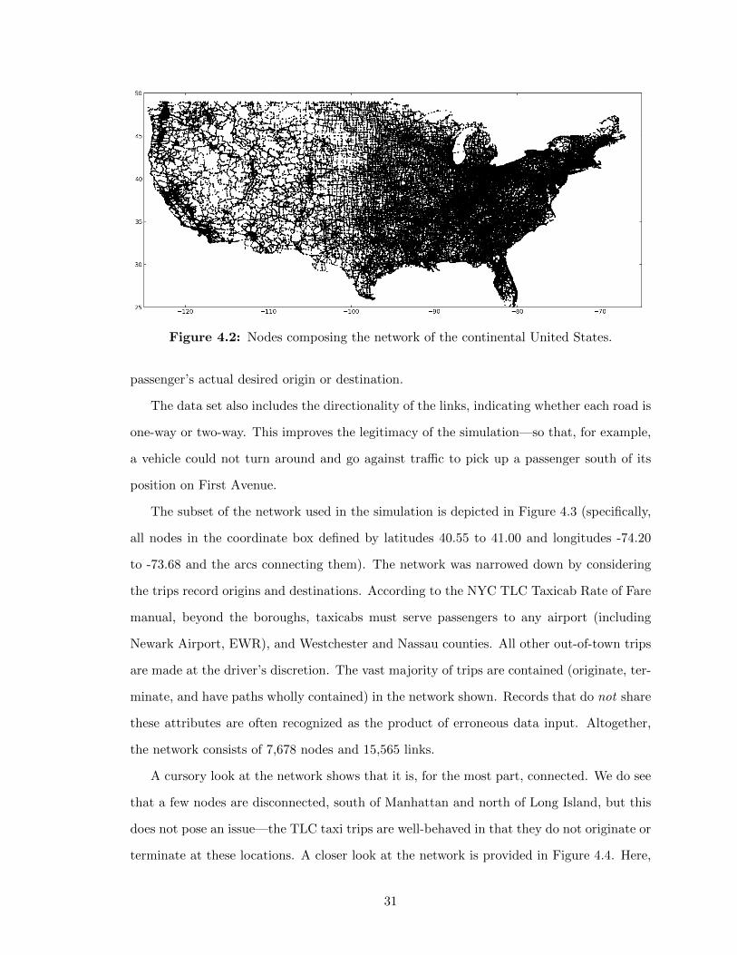
Figure 4.2: Nodes composing the network of the continental United States.

passenger’s actual desired origin or destination.

The data set also includes the directionality of the links, indicating whether each road is

one-way or two-way. This improves the legitimacy of the simulation—so that, for example,

a vehicle could not turn around and go against traffic to pick up a passenger south of its

position on First Avenue.

The subset of the network used in the simulation is depicted in Figure 4.3 (specifically,

all nodes in the coordinate box defined by latitudes 40.55 to 41.00 and longitudes -74.20

to -73.68 and the arcs connecting them). The network was narrowed down by considering

the trips record origins and destinations. According to the NYC TLC Taxicab Rate of Fare

manual, beyond the boroughs, taxicabs must serve passengers to any airport (including

Newark Airport, EWR), and Westchester and Nassau counties. All other out-of-town trips

are made at the driver’s discretion. The vast majority of trips are contained (originate, ter-

minate, and have paths wholly contained) in the network shown. Records that do not share

these attributes are often recognized as the product of erroneous data input. Altogether,

the network consists of 7,678 nodes and 15,565 links.

A cursory look at the network shows that it is, for the most part, connected. We do see

that a few nodes are disconnected, south of Manhattan and north of Long Island, but this

does not pose an issue—the TLC taxi trips are well-behaved in that they do not originate or

terminate at these locations. A closer look at the network is provided in Figure 4.4. Here,

31

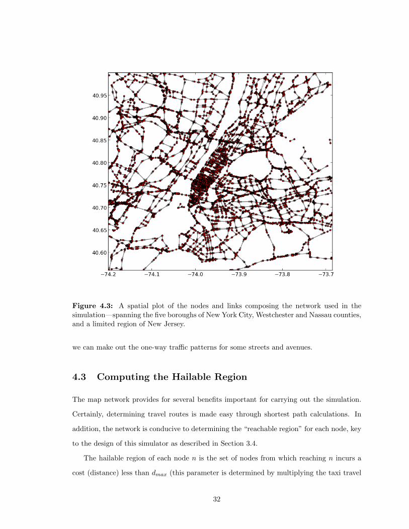
Figure 4.3: A spatial plot of the nodes and links composing the network used in thesimulation—spanning the five boroughs of New York City, Westchester and Nassau counties,and a limited region of New Jersey.

we can make out the one-way traffic patterns for some streets and avenues.

4.3 Computing the Hailable Region

The map network provides for several benefits important for carrying out the simulation.

Certainly, determining travel routes is made easy through shortest path calculations. In

addition, the network is conducive to determining the “reachable region” for each node, key

to the design of this simulator as described in Section 3.4.

The hailable region of each node n is the set of nodes from which reaching n incurs a

cost (distance) less than dmax (this parameter is determined by multiplying the taxi travel

32

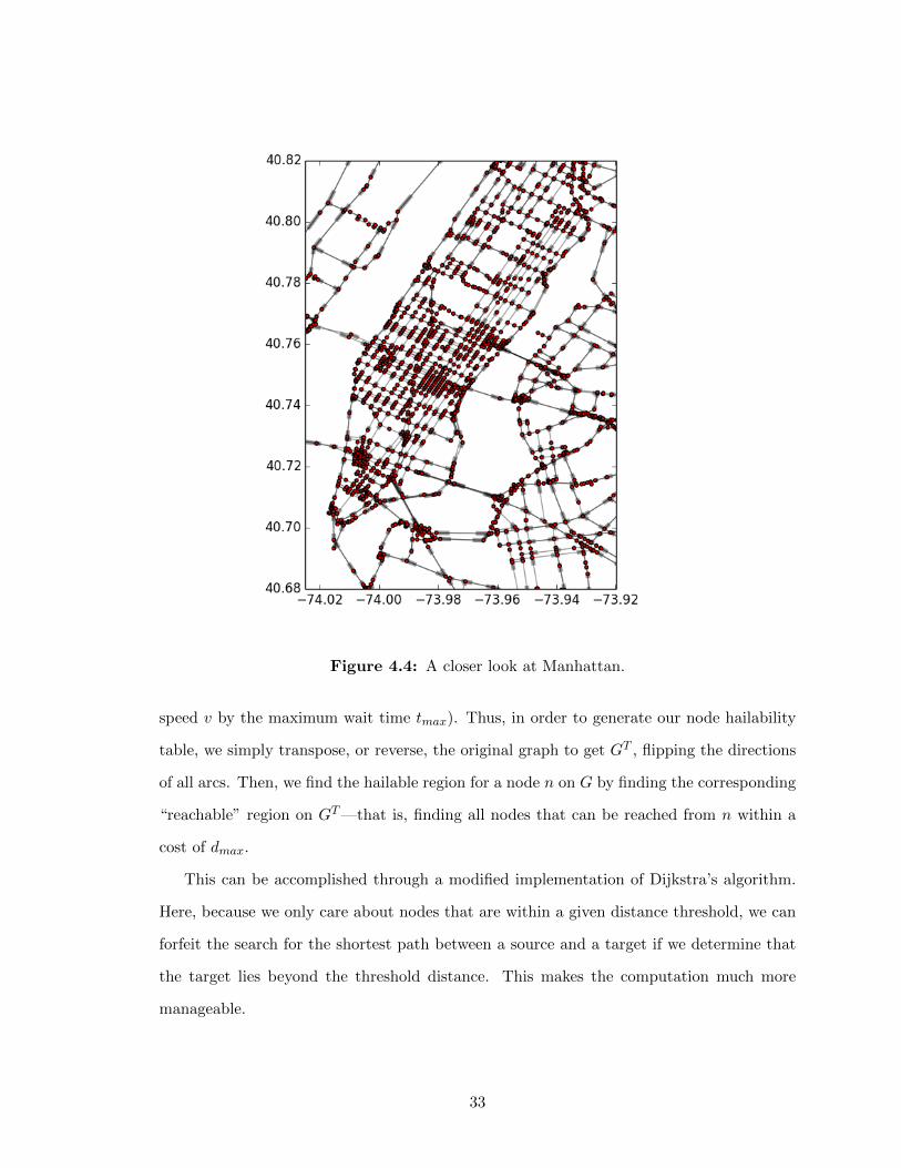
Figure 4.4: A closer look at Manhattan.

speed v by the maximum wait time tmax). Thus, in order to generate our node hailability

table, we simply transpose, or reverse, the original graph to get GT , flipping the directions

of all arcs. Then, we find the hailable region for a node n on G by finding the corresponding

“reachable” region on GT—that is, finding all nodes that can be reached from n within a

cost of dmax.

This can be accomplished through a modified implementation of Dijkstra’s algorithm.

Here, because we only care about nodes that are within a given distance threshold, we can

forfeit the search for the shortest path between a source and a target if we determine that

the target lies beyond the threshold distance. This makes the computation much more

manageable.

33

4.4 Mapping Rides to Nodes

Each TLC trip record contains origin and destination latitude-longitude coordinates. In

order to place the trips on the network, each origin and destination position was mapped

to the nearest node on the New York City graph shown in Figure 4.3. The conceptual

implication here is that each passenger would walk from his or her “true” origin (the lati-

tude/longitude coordinate of the trip record) to the nearest node for pick-up, and from the

drop-off node to his or her “true” destination.

This two-dimensional nearest-neighbor search was carried out using a k-d tree data

structure. This result offers an origin and destination node for each trip record, as well as

the distance each individual must walk to the origin node or from the destination node.

As a technical detail, it is important to note that this implementation does not use

the great circle distance (typically used for finding the distance between two points on

a sphere) to map the trips or determine walking distances. Rather, it assumes that we

are working over a sufficiently small area, and the nodes are sufficiently well distributed

across the region, that we can approximate the path from trip coordinate to node to be

flat (rather than curved). Thus, the mappings are based on Cartesian distances. Indeed,

simply examining the spatial plot of the network reveals that there is no point on land that

is so far away from a node as to render this approximation an issue.

From this data pre-processing step, trips with faulty data became easy to pick out and

eliminate from the simulation, as the calculated distance to pick-up or from drop-off was

unreasonably high. Individual inspection of these records often revealed, for example, that

they originated in the Atlantic Ocean, or terminated in non-adjacent state. In other cases,

trips simply originated or terminated too far from the area of focus to warrant consideration.

4.5 A Note on Runtime

The simulator in its present form serves as a example of the importance of efficient program-

ming. The first iteration of the simulation program required 4 days to run through a week’s

worth of trip data—while it achieved the correct end result through a deterministic compu-

tation, it was simply not scalable to larger trip record sets (say, a month, and certainly not a

34

year). In order to address the need to run multiple simulations, it was necessary to pinpoint

and eliminate the bottleneck in the code. Specifically, while each shortest path computa-

tion is, on its own, relatively uncostly, the sheer scale on which this algorithm was being

called rendered the program greatly inefficient. A simple caching strategy—preemptively

calculating the shortest path length between each pair of nodes in the network and storing

them in an N by N matrix (where N = 7678, the number of nodes in the network)—

drastically reduced the runtime of the simulation to a matter of hours. I include this note

here to demonstrate the difficulty of dealing with a large (but realistically sized) dataset

and network—and to emphasize the importance of careful programming.

35

Chapter 5

Examination of Trip Record Data

While the simulation is designed to run over an arbitrarily long trip record set, it is limited

by constraints on time. A small time step, millions of passengers, thousands of taxis, and an

exhaustive taxi-assignment search are complications that align to create a computationally

burdensome task. Further, because the state of the system at time t+1 is entirely dependent

on its state at t, the code is not advantageously parallelizable. With this constraint on

time, the data sample was limited to just one week’s worth of TLC trip records, specifically

encompassing all demand arising between January 7 and January 13, 2015.

In this chapter, prior to examining the results of the simulation, we take a closer look at

the trip records from the sampled week to gain insight into the patterns and characteristics

they exhibit. Specifically, this chapter reveals how trips are distributed before and after

they are mapped to the network, both temporally (which times of day are busiest) and

spatially (which areas of the city see the most passenger traffic).

As a technical detail, all trips that began within this time window were completed—that

is, all passengers that requested a taxi in the late hours of January 13th were accommodated,

even if they were dropped off in the early hours of the 14th. However, rides that originated

on January 6th and terminated on the 7th were not considered.

36

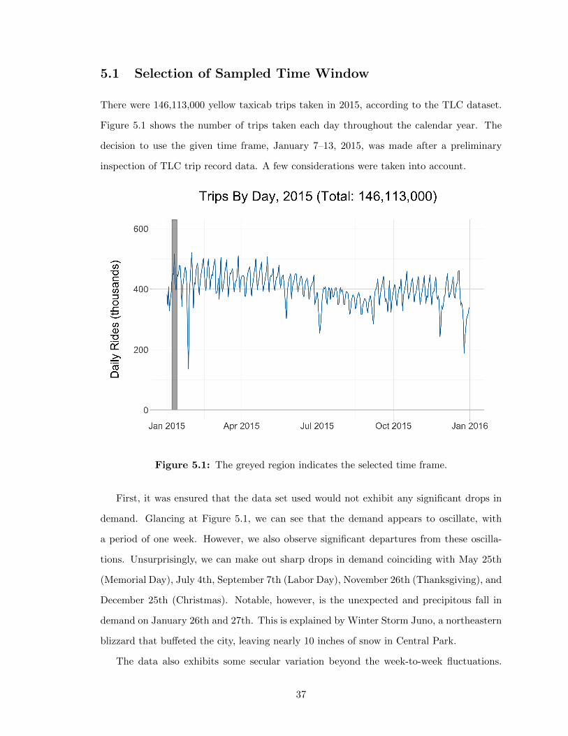
5.1 Selection of Sampled Time Window

There were 146,113,000 yellow taxicab trips taken in 2015, according to the TLC dataset.

Figure 5.1 shows the number of trips taken each day throughout the calendar year. The

decision to use the given time frame, January 7–13, 2015, was made after a preliminary

inspection of TLC trip record data. A few considerations were taken into account.

Figure 5.1: The greyed region indicates the selected time frame.

First, it was ensured that the data set used would not exhibit any significant drops in

demand. Glancing at Figure 5.1, we can see that the demand appears to oscillate, with

a period of one week. However, we also observe significant departures from these oscilla-

tions. Unsurprisingly, we can make out sharp drops in demand coinciding with May 25th

(Memorial Day), July 4th, September 7th (Labor Day), November 26th (Thanksgiving), and

December 25th (Christmas). Notable, however, is the unexpected and precipitous fall in

demand on January 26th and 27th. This is explained by Winter Storm Juno, a northeastern

blizzard that buffeted the city, leaving nearly 10 inches of snow in Central Park.

The data also exhibits some secular variation beyond the week-to-week fluctuations.

37

Stretching from the beginning of January through the end of April, we observe that demand

oscillates around 450,000 trips per day. After this, there is a gradual decline through the

summer months into September, when a slight uptick settles the oscillations around 400,000

trips per day. The cause of this trend remains unclear.

I chose to sample a week from the earlier phase of the year, so as to simulate a situation

with more demand. We may expect that might favorably bias our simulated average vehicle

occupancy (more trips presumably translates into more ride-share opportunities)—however,

it is important to ensure that the proposed framework for accommodating trips is able to

appropriately service the highest levels of demand. That is, we err on the side of over-

preparedness. The selected week posted the second highest single-day demand of the year

at 515,000 trips (surpassed only by the day the streets were cleared in the aftermath of

Juno, with 520,000)—ideal for testing the limits of the system.

A more nuanced decision made regarding the sampled week was determining the start

and end points. We may be naturally inclined to simply choose a traditional seven-day block

beginning on a Sunday or a Monday. However, a break between Saturday and Sunday would

disrupt the stream of late night Saturday trips, which make up a significant proportion of

weekend activity. Why not Monday then? We might imagine that the workweek starts off

with some “lag” from a transportation perspective. Individuals may be flying into the city

for work from out of town, or perhaps they might take a day off to extend their weekend

plans. The scale of these details and the effect (if any) they might have on trips are not

clear. However, it is uncontroversial to choose a mid-week day, say Wednesday, as the

starting point. For this reason, the sampled week begins on a Wednesday and ends the

following Tuesday.

5.2 Temporal Distribution

The sampled week consists of 3,045,787 trips, representing just over 2% of the trips made

in 2015. Out of these raw trip records, 42,347 (or about 1.4% of the sampled trips) were

“tossed out,” either because they had pick-up or drop-off locations mapped to a node not

on the simulation network (whose nodes are depicted in Figure 4.3) or because the network

38

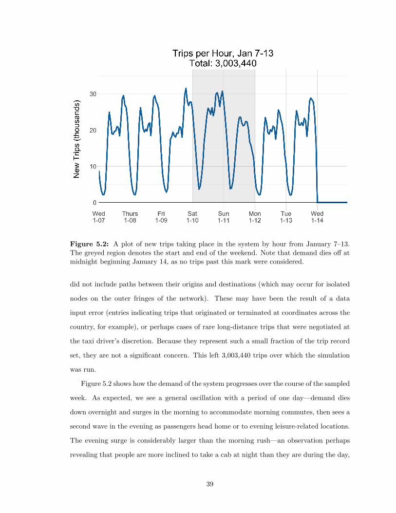
Figure 5.2: A plot of new trips taking place in the system by hour from January 7–13.The greyed region denotes the start and end of the weekend. Note that demand dies off atmidnight beginning January 14, as no trips past this mark were considered.

did not include paths between their origins and destinations (which may occur for isolated

nodes on the outer fringes of the network). These may have been the result of a data

input error (entries indicating trips that originated or terminated at coordinates across the

country, for example), or perhaps cases of rare long-distance trips that were negotiated at

the taxi driver’s discretion. Because they represent such a small fraction of the trip record

set, they are not a significant concern. This left 3,003,440 trips over which the simulation

was run.

Figure 5.2 shows how the demand of the system progresses over the course of the sampled

week. As expected, we see a general oscillation with a period of one day—demand dies

down overnight and surges in the morning to accommodate morning commutes, then sees a

second wave in the evening as passengers head home or to evening leisure-related locations.

The evening surge is considerably larger than the morning rush—an observation perhaps

revealing that people are more inclined to take a cab at night than they are during the day,

39

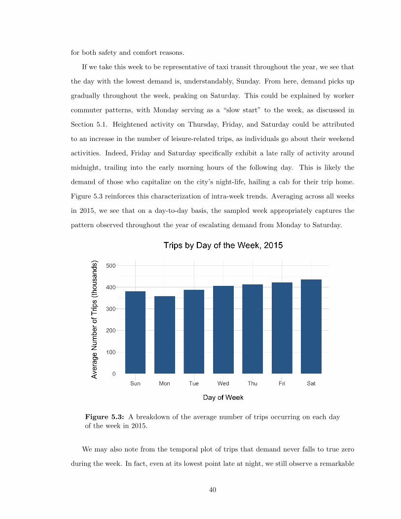
for both safety and comfort reasons.

If we take this week to be representative of taxi transit throughout the year, we see that

the day with the lowest demand is, understandably, Sunday. From here, demand picks up

gradually throughout the week, peaking on Saturday. This could be explained by worker

commuter patterns, with Monday serving as a “slow start” to the week, as discussed in

Section 5.1. Heightened activity on Thursday, Friday, and Saturday could be attributed

to an increase in the number of leisure-related trips, as individuals go about their weekend

activities. Indeed, Friday and Saturday specifically exhibit a late rally of activity around

midnight, trailing into the early morning hours of the following day. This is likely the

demand of those who capitalize on the city’s night-life, hailing a cab for their trip home.

Figure 5.3 reinforces this characterization of intra-week trends. Averaging across all weeks

in 2015, we see that on a day-to-day basis, the sampled week appropriately captures the

pattern observed throughout the year of escalating demand from Monday to Saturday.

Figure 5.3: A breakdown of the average number of trips occurring on each dayof the week in 2015.

We may also note from the temporal plot of trips that demand never falls to true zero

during the week. In fact, even at its lowest point late at night, we still observe a remarkable

40

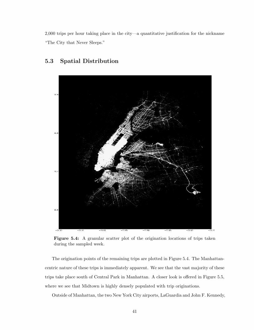
2,000 trips per hour taking place in the city—a quantitative justification for the nickname

“The City that Never Sleeps.”

5.3 Spatial Distribution

Figure 5.4: A granular scatter plot of the origination locations of trips takenduring the sampled week.

The origination points of the remaining trips are plotted in Figure 5.4. The Manhattan-

centric nature of these trips is immediately apparent. We see that the vast majority of these

trips take place south of Central Park in Manhattan. A closer look is offered in Figure 5.5,

where we see that Midtown is highly densely populated with trip originations.

Outside of Manhattan, the two New York City airports, LaGuardia and John F. Kennedy,

41

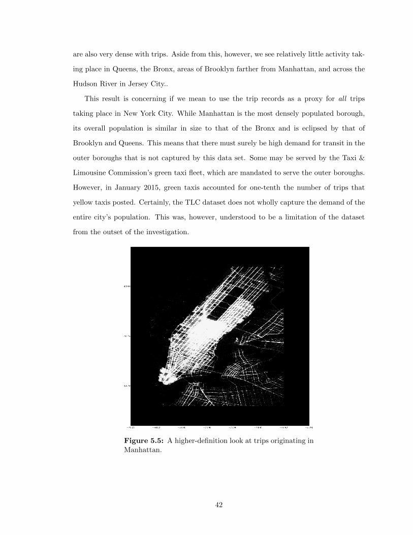
are also very dense with trips. Aside from this, however, we see relatively little activity tak-

ing place in Queens, the Bronx, areas of Brooklyn farther from Manhattan, and across the

Hudson River in Jersey City..

This result is concerning if we mean to use the trip records as a proxy for all trips

taking place in New York City. While Manhattan is the most densely populated borough,

its overall population is similar in size to that of the Bronx and is eclipsed by that of

Brooklyn and Queens. This means that there must surely be high demand for transit in the

outer boroughs that is not captured by this data set. Some may be served by the Taxi &

Limousine Commission’s green taxi fleet, which are mandated to serve the outer boroughs.

However, in January 2015, green taxis accounted for one-tenth the number of trips that

yellow taxis posted. Certainly, the TLC dataset does not wholly capture the demand of the

entire city’s population. This was, however, understood to be a limitation of the dataset

from the outset of the investigation.

Figure 5.5: A higher-definition look at trips originating inManhattan.

42

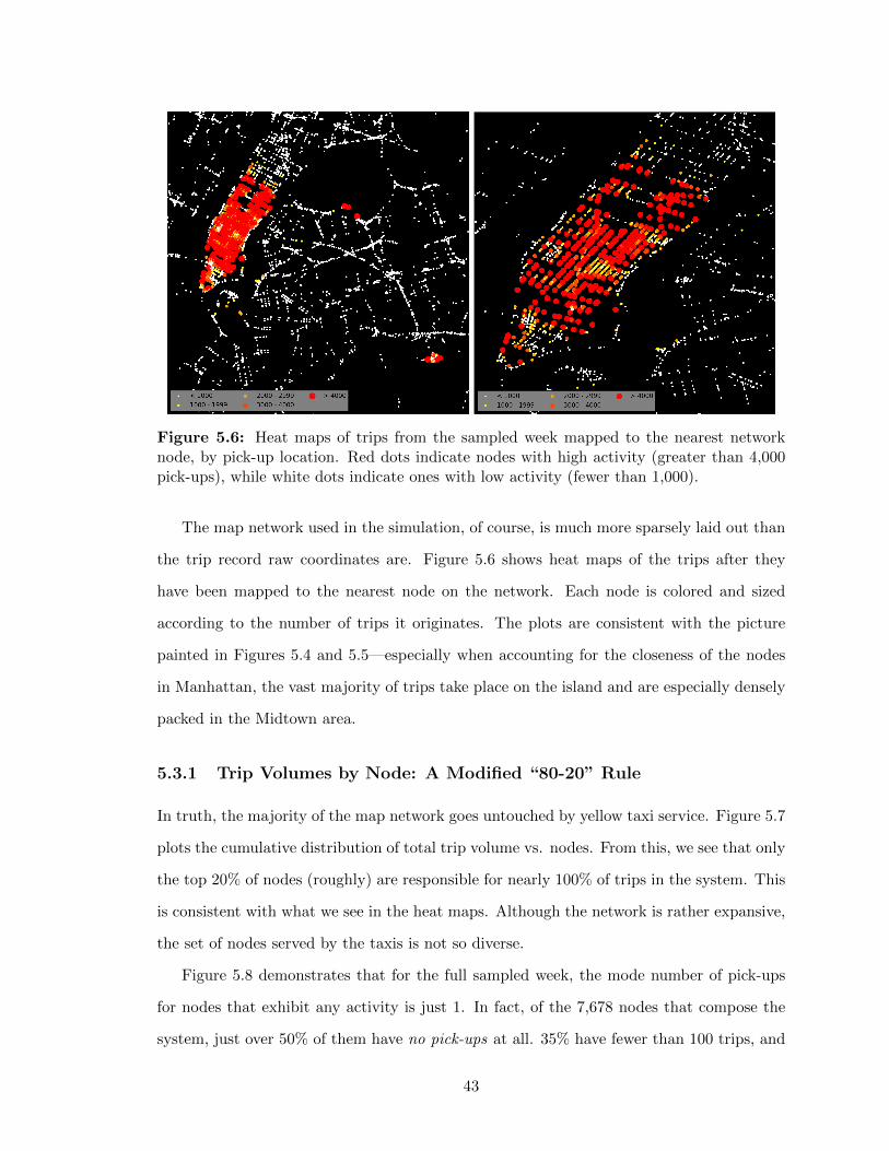
Figure 5.6: Heat maps of trips from the sampled week mapped to the nearest networknode, by pick-up location. Red dots indicate nodes with high activity (greater than 4,000pick-ups), while white dots indicate ones with low activity (fewer than 1,000).

The map network used in the simulation, of course, is much more sparsely laid out than

the trip record raw coordinates are. Figure 5.6 shows heat maps of the trips after they

have been mapped to the nearest node on the network. Each node is colored and sized

according to the number of trips it originates. The plots are consistent with the picture

painted in Figures 5.4 and 5.5—especially when accounting for the closeness of the nodes

in Manhattan, the vast majority of trips take place on the island and are especially densely

packed in the Midtown area.

5.3.1 Trip Volumes by Node: A Modified “80-20” Rule

In truth, the majority of the map network goes untouched by yellow taxi service. Figure 5.7

plots the cumulative distribution of total trip volume vs. nodes. From this, we see that only

the top 20% of nodes (roughly) are responsible for nearly 100% of trips in the system. This

is consistent with what we see in the heat maps. Although the network is rather expansive,

the set of nodes served by the taxis is not so diverse.

Figure 5.8 demonstrates that for the full sampled week, the mode number of pick-ups

for nodes that exhibit any activity is just 1. In fact, of the 7,678 nodes that compose the

system, just over 50% of them have no pick-ups at all. 35% have fewer than 100 trips, and

43

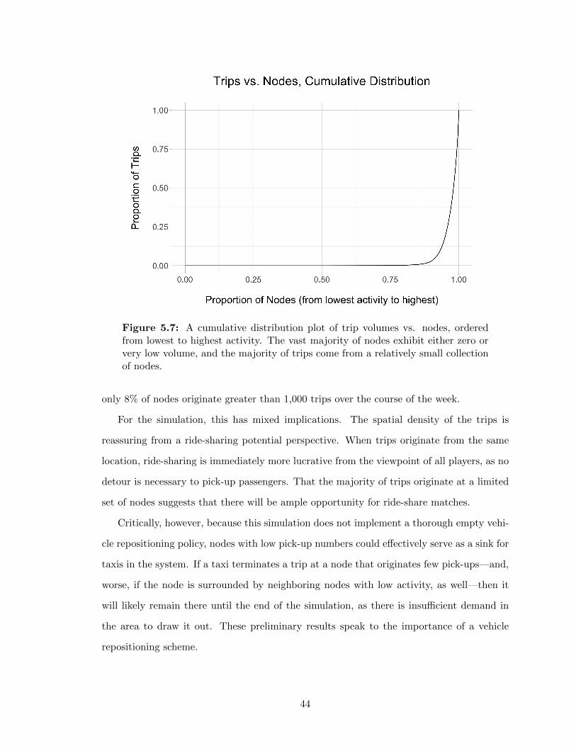
Figure 5.7: A cumulative distribution plot of trip volumes vs. nodes, orderedfrom lowest to highest activity. The vast majority of nodes exhibit either zero orvery low volume, and the majority of trips come from a relatively small collectionof nodes.

only 8% of nodes originate greater than 1,000 trips over the course of the week.

For the simulation, this has mixed implications. The spatial density of the trips is

reassuring from a ride-sharing potential perspective. When trips originate from the same

location, ride-sharing is immediately more lucrative from the viewpoint of all players, as no

detour is necessary to pick-up passengers. That the majority of trips originate at a limited

set of nodes suggests that there will be ample opportunity for ride-share matches.

Critically, however, because this simulation does not implement a thorough empty vehi-

cle repositioning policy, nodes with low pick-up numbers could effectively serve as a sink for

taxis in the system. If a taxi terminates a trip at a node that originates few pick-ups—and,

worse, if the node is surrounded by neighboring nodes with low activity, as well—then it

will likely remain there until the end of the simulation, as there is insufficient demand in

the area to draw it out. These preliminary results speak to the importance of a vehicle

repositioning scheme.

44

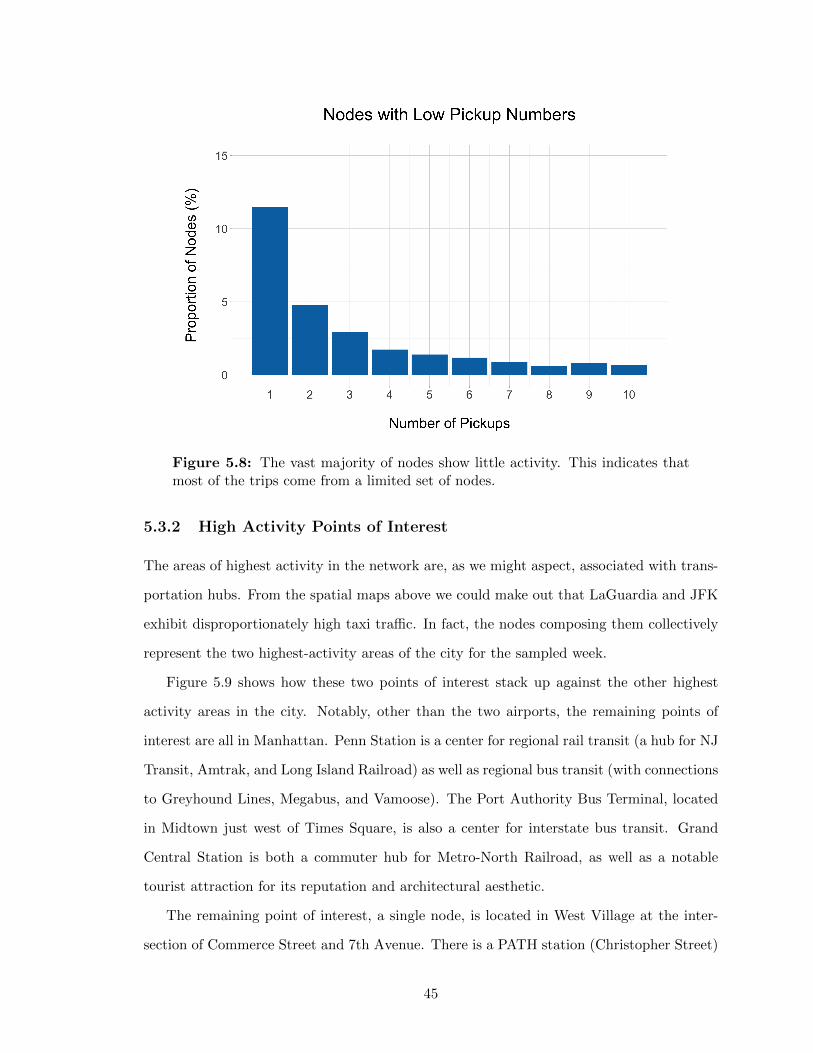
Figure 5.8: The vast majority of nodes show little activity. This indicates thatmost of the trips come from a limited set of nodes.

5.3.2 High Activity Points of Interest

The areas of highest activity in the network are, as we might aspect, associated with trans-

portation hubs. From the spatial maps above we could make out that LaGuardia and JFK

exhibit disproportionately high taxi traffic. In fact, the nodes composing them collectively

represent the two highest-activity areas of the city for the sampled week.

Figure 5.9 shows how these two points of interest stack up against the other highest

activity areas in the city. Notably, other than the two airports, the remaining points of

interest are all in Manhattan. Penn Station is a center for regional rail transit (a hub for NJ

Transit, Amtrak, and Long Island Railroad) as well as regional bus transit (with connections

to Greyhound Lines, Megabus, and Vamoose). The Port Authority Bus Terminal, located

in Midtown just west of Times Square, is also a center for interstate bus transit. Grand

Central Station is both a commuter hub for Metro-North Railroad, as well as a notable

tourist attraction for its reputation and architectural aesthetic.

The remaining point of interest, a single node, is located in West Village at the inter-

section of Commerce Street and 7th Avenue. There is a PATH station (Christopher Street)

45

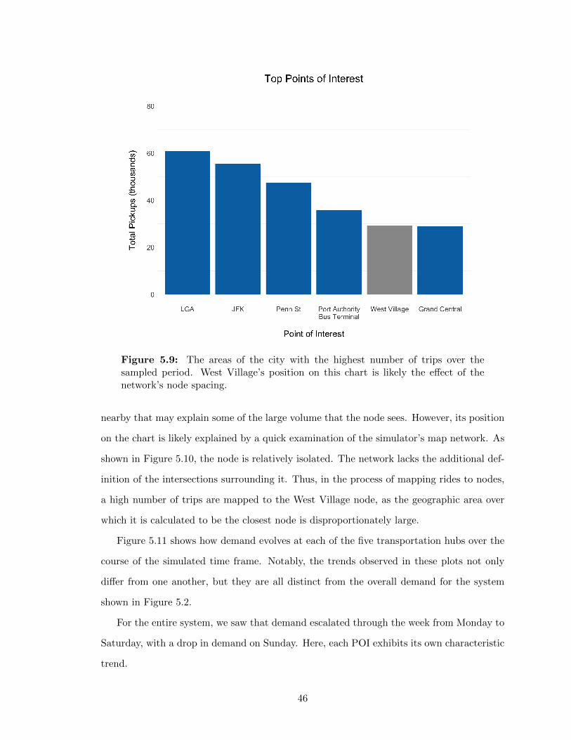
Figure 5.9: The areas of the city with the highest number of trips over thesampled period. West Village’s position on this chart is likely the effect of thenetwork’s node spacing.

nearby that may explain some of the large volume that the node sees. However, its position

on the chart is likely explained by a quick examination of the simulator’s map network. As

shown in Figure 5.10, the node is relatively isolated. The network lacks the additional def-

inition of the intersections surrounding it. Thus, in the process of mapping rides to nodes,

a high number of trips are mapped to the West Village node, as the geographic area over

which it is calculated to be the closest node is disproportionately large.

Figure 5.11 shows how demand evolves at each of the five transportation hubs over the

course of the simulated time frame. Notably, the trends observed in these plots not only

differ from one another, but they are all distinct from the overall demand for the system

shown in Figure 5.2.

For the entire system, we saw that demand escalated through the week from Monday to

Saturday, with a drop in demand on Sunday. Here, each POI exhibits its own characteristic

trend.

46

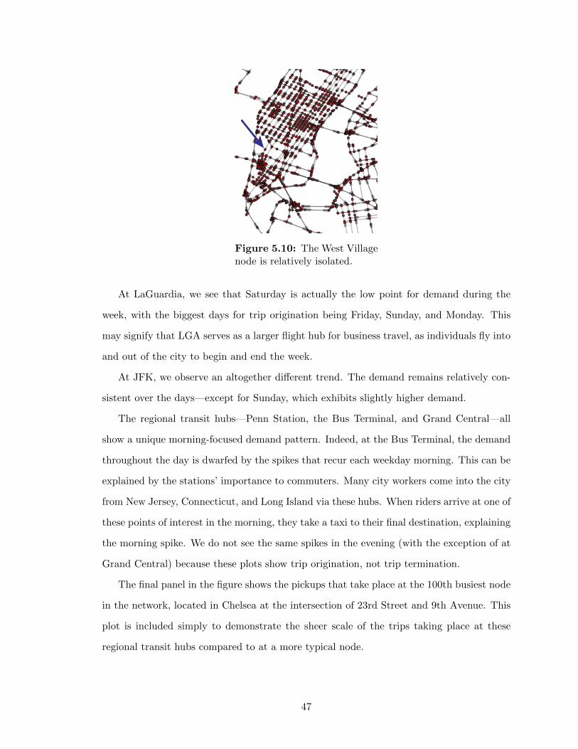
Figure 5.10: The West Villagenode is relatively isolated.

At LaGuardia, we see that Saturday is actually the low point for demand during the

week, with the biggest days for trip origination being Friday, Sunday, and Monday. This

may signify that LGA serves as a larger flight hub for business travel, as individuals fly into

and out of the city to begin and end the week.

At JFK, we observe an altogether different trend. The demand remains relatively con-

sistent over the days—except for Sunday, which exhibits slightly higher demand.

The regional transit hubs—Penn Station, the Bus Terminal, and Grand Central—all

show a unique morning-focused demand pattern. Indeed, at the Bus Terminal, the demand

throughout the day is dwarfed by the spikes that recur each weekday morning. This can be

explained by the stations’ importance to commuters. Many city workers come into the city

from New Jersey, Connecticut, and Long Island via these hubs. When riders arrive at one of

these points of interest in the morning, they take a taxi to their final destination, explaining

the morning spike. We do not see the same spikes in the evening (with the exception of at

Grand Central) because these plots show trip origination, not trip termination.

The final panel in the figure shows the pickups that take place at the 100th busiest node

in the network, located in Chelsea at the intersection of 23rd Street and 9th Avenue. This

plot is included simply to demonstrate the sheer scale of the trips taking place at these

regional transit hubs compared to at a more typical node.

47

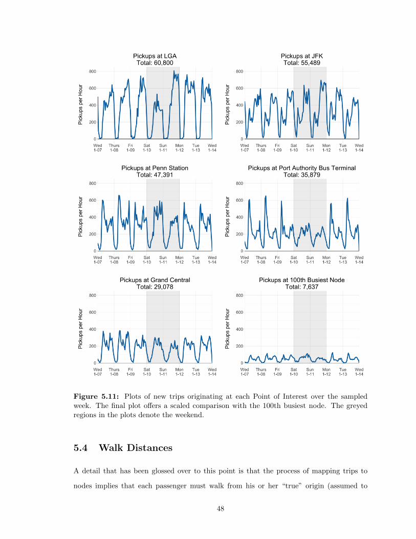
Figure 5.11: Plots of new trips originating at each Point of Interest over the sampledweek. The final plot offers a scaled comparison with the 100th busiest node. The greyedregions in the plots denote the weekend.

5.4 Walk Distances

A detail that has been glossed over to this point is that the process of mapping trips to

nodes implies that each passenger must walk from his or her “true” origin (assumed to

48

be the latitude/longitude coordinate of the trip record) to the nearest network node for

pick-up, and from the drop-off point to his or her “true” destination. These distances were

calculated using a Euclidean distance approximation, as described in Section 4.4.

The distributions of walking distances shown in Figures 5.12 and 5.13 demonstrate

that the vast majority of record mappings (roughly 80%) require passengers to walk no

more than one-tenth of a mile on either end of their trip (to pick-up or from drop-off), a

reassuringly short distance. These distributions do exhibit fairly large tails—240 records

require a walking distance to pick-up of greater than 1 mile, and 75 require greater than

3 miles. Most of these originate on the fringes of the network, where the nodes are more

spaced out. However, they represent less than 0.01% of all trips, so we do not consider them

an issue here.

49

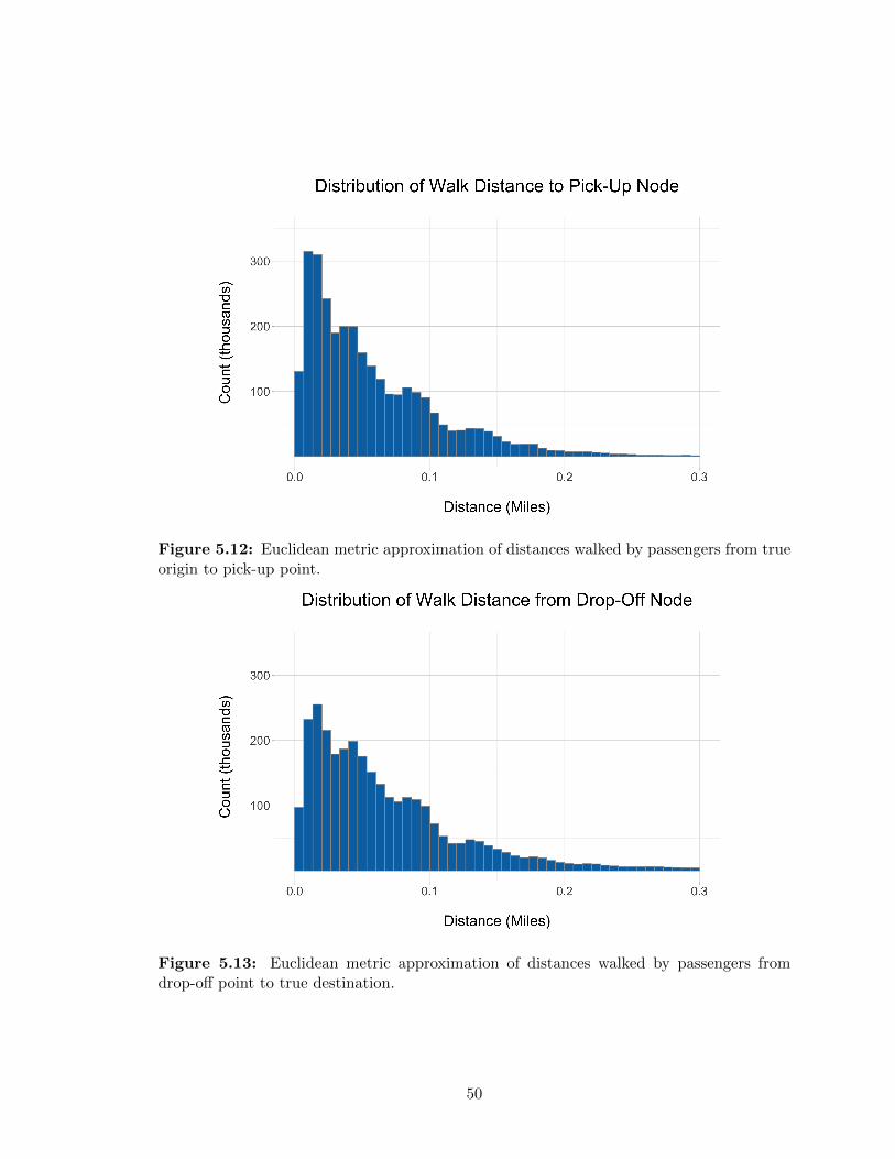
Figure 5.12: Euclidean metric approximation of distances walked by passengers from trueorigin to pick-up point.

Figure 5.13: Euclidean metric approximation of distances walked by passengers fromdrop-off point to true destination.

50

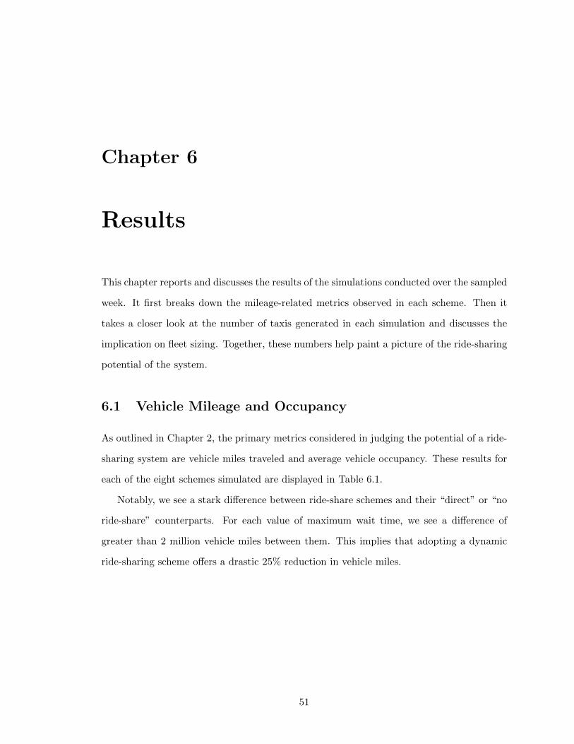
Chapter 6

Results

This chapter reports and discusses the results of the simulations conducted over the sampled

week. It first breaks down the mileage-related metrics observed in each scheme. Then it

takes a closer look at the number of taxis generated in each simulation and discusses the

implication on fleet sizing. Together, these numbers help paint a picture of the ride-sharing

potential of the system.

6.1 Vehicle Mileage and Occupancy

As outlined in Chapter 2, the primary metrics considered in judging the potential of a ride-

sharing system are vehicle miles traveled and average vehicle occupancy. These results for

each of the eight schemes simulated are displayed in Table 6.1.

Notably, we see a stark difference between ride-share schemes and their “direct” or “no

ride-share” counterparts. For each value of maximum wait time, we see a difference of

greater than 2 million vehicle miles between them. This implies that adopting a dynamic

ride-sharing scheme offers a drastic 25% reduction in vehicle miles.

51

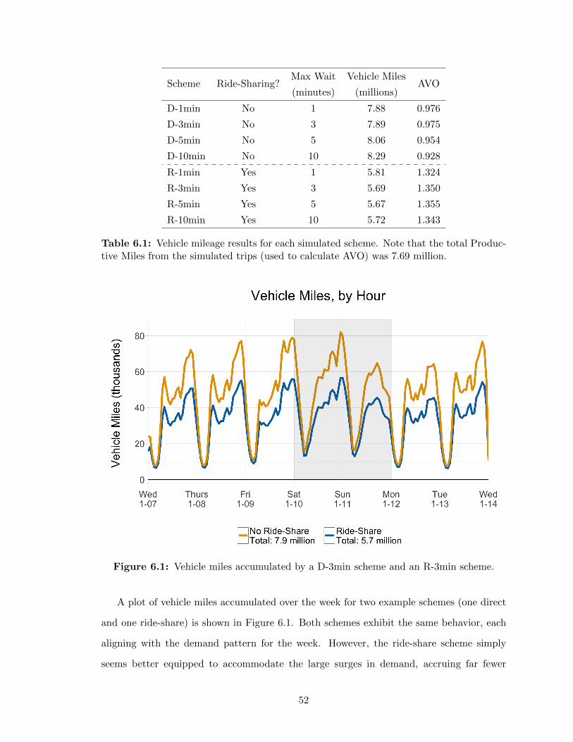
Scheme Ride-Sharing?Max Wait

(minutes)

Vehicle Miles

(millions)AVO

D-1min No 1 7.88 0.976

D-3min No 3 7.89 0.975

D-5min No 5 8.06 0.954

D-10min No 10 8.29 0.928

R-1min Yes 1 5.81 1.324

R-3min Yes 3 5.69 1.350

R-5min Yes 5 5.67 1.355

R-10min Yes 10 5.72 1.343

Table 6.1: Vehicle mileage results for each simulated scheme. Note that the total Produc-tive Miles from the simulated trips (used to calculate AVO) was 7.69 million.

Figure 6.1: Vehicle miles accumulated by a D-3min scheme and an R-3min scheme.

A plot of vehicle miles accumulated over the week for two example schemes (one direct

and one ride-share) is shown in Figure 6.1. Both schemes exhibit the same behavior, each

aligning with the demand pattern for the week. However, the ride-share scheme simply

seems better equipped to accommodate the large surges in demand, accruing far fewer

52

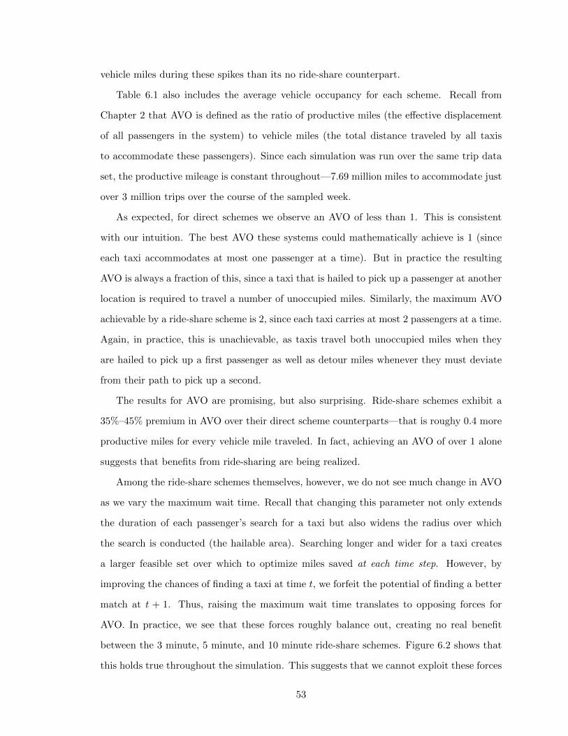
vehicle miles during these spikes than its no ride-share counterpart.

Table 6.1 also includes the average vehicle occupancy for each scheme. Recall from

Chapter 2 that AVO is defined as the ratio of productive miles (the effective displacement

of all passengers in the system) to vehicle miles (the total distance traveled by all taxis

to accommodate these passengers). Since each simulation was run over the same trip data

set, the productive mileage is constant throughout—7.69 million miles to accommodate just

over 3 million trips over the course of the sampled week.

As expected, for direct schemes we observe an AVO of less than 1. This is consistent

with our intuition. The best AVO these systems could mathematically achieve is 1 (since

each taxi accommodates at most one passenger at a time). But in practice the resulting

AVO is always a fraction of this, since a taxi that is hailed to pick up a passenger at another

location is required to travel a number of unoccupied miles. Similarly, the maximum AVO

achievable by a ride-share scheme is 2, since each taxi carries at most 2 passengers at a time.

Again, in practice, this is unachievable, as taxis travel both unoccupied miles when they

are hailed to pick up a first passenger as well as detour miles whenever they must deviate

from their path to pick up a second.

The results for AVO are promising, but also surprising. Ride-share schemes exhibit a

35%–45% premium in AVO over their direct scheme counterparts—that is roughy 0.4 more

productive miles for every vehicle mile traveled. In fact, achieving an AVO of over 1 alone

suggests that benefits from ride-sharing are being realized.

Among the ride-share schemes themselves, however, we do not see much change in AVO

as we vary the maximum wait time. Recall that changing this parameter not only extends

the duration of each passenger’s search for a taxi but also widens the radius over which

the search is conducted (the hailable area). Searching longer and wider for a taxi creates

a larger feasible set over which to optimize miles saved at each time step. However, by

improving the chances of finding a taxi at time t, we forfeit the potential of finding a better

match at t + 1. Thus, raising the maximum wait time translates to opposing forces for

AVO. In practice, we see that these forces roughly balance out, creating no real benefit

between the 3 minute, 5 minute, and 10 minute ride-share schemes. Figure 6.2 shows that

this holds true throughout the simulation. This suggests that we cannot exploit these forces

53

to improve AVO by varying the wait time at different times of day, as the trade-off is being

made continuously, regardless of demand levels.

Figure 6.2: The AVO for each ride-share scheme plotted over the sampled week.

6.2 Trips Shared and Fleet Sizing

Also discussed in Chapter 2 is the importance of taxi fleet size, as it represents a significant

fixed cost in the operation. Table 6.2 displays the fleet size of each simulation, along with

AVO and ride-sharing percentage (the proportion of all trips that were shared for some part

of the journey) in order to more holistically judge ride-sharing potential.

54

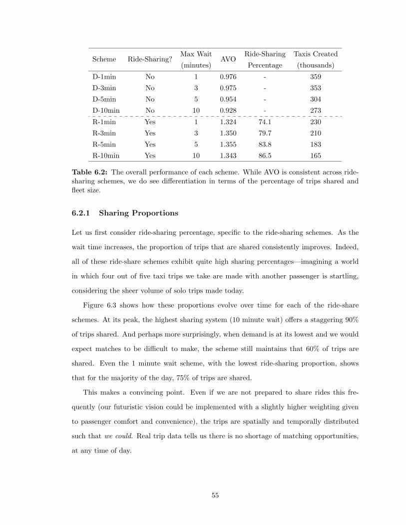
Scheme Ride-Sharing?Max Wait

(minutes)AVO

Ride-Sharing

Percentage

Taxis Created

(thousands)

D-1min No 1 0.976 - 359

D-3min No 3 0.975 - 353

D-5min No 5 0.954 - 304

D-10min No 10 0.928 - 273

R-1min Yes 1 1.324 74.1 230

R-3min Yes 3 1.350 79.7 210

R-5min Yes 5 1.355 83.8 183

R-10min Yes 10 1.343 86.5 165

Table 6.2: The overall performance of each scheme. While AVO is consistent across ride-sharing schemes, we do see differentiation in terms of the percentage of trips shared andfleet size.

6.2.1 Sharing Proportions

Let us first consider ride-sharing percentage, specific to the ride-sharing schemes. As the

wait time increases, the proportion of trips that are shared consistently improves. Indeed,

all of these ride-share schemes exhibit quite high sharing percentages—imagining a world

in which four out of five taxi trips we take are made with another passenger is startling,

considering the sheer volume of solo trips made today.

Figure 6.3 shows how these proportions evolve over time for each of the ride-share

schemes. At its peak, the highest sharing system (10 minute wait) offers a staggering 90%

of trips shared. And perhaps more surprisingly, when demand is at its lowest and we would

expect matches to be difficult to make, the scheme still maintains that 60% of trips are

shared. Even the 1 minute wait scheme, with the lowest ride-sharing proportion, shows

that for the majority of the day, 75% of trips are shared.

This makes a convincing point. Even if we are not prepared to share rides this fre-

quently (our futuristic vision could be implemented with a slightly higher weighting given

to passenger comfort and convenience), the trips are spatially and temporally distributed

such that we could. Real trip data tells us there is no shortage of matching opportunities,

at any time of day.

55

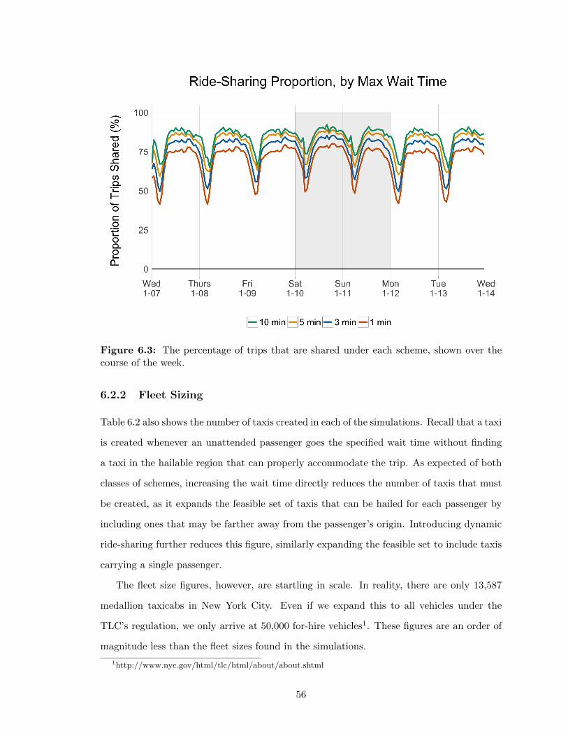
Figure 6.3: The percentage of trips that are shared under each scheme, shown over thecourse of the week.

6.2.2 Fleet Sizing

Table 6.2 also shows the number of taxis created in each of the simulations. Recall that a taxi

is created whenever an unattended passenger goes the specified wait time without finding

a taxi in the hailable region that can properly accommodate the trip. As expected of both

classes of schemes, increasing the wait time directly reduces the number of taxis that must

be created, as it expands the feasible set of taxis that can be hailed for each passenger by

including ones that may be farther away from the passenger’s origin. Introducing dynamic

ride-sharing further reduces this figure, similarly expanding the feasible set to include taxis

carrying a single passenger.

The fleet size figures, however, are startling in scale. In reality, there are only 13,587

medallion taxicabs in New York City. Even if we expand this to all vehicles under the

TLC’s regulation, we only arrive at 50,000 for-hire vehicles1. These figures are an order of

magnitude less than the fleet sizes found in the simulations.

1http://www.nyc.gov/html/tlc/html/about/about.shtml

56

The cause of this misestimation is clear, and has been stressed throughout this study:

the simulation does not incorporate or implement an effective empty vehicle repositioning

strategy. As considered in Chapter 4, if a taxi is not repositioned after completing a trip,

it requires a trip to spawn at or near its location be pulled into service again. Thus, taxis

completing trips in areas of lower demand may be fixed there for a lengthened period of

time, as a trip that will “draw it out” of its location is unlikely to emerge soon. In this

case, the effective size of the taxi fleet, and its ability to serve demand across the network,

is reduced.

What had not been expected prior to carrying out the simulation is that areas of high

demand would be equally responsible for skewing the fleet size. When surges of demand

come up, these areas force the rapid creation of taxis, as the supply in the surrounding area

is rapidly depleted and the maximum wait time for unattended passengers passes before a

sufficient number of trips can come in.

Plots of the net taxi inflow and outflow per hour for the 3 minute ride-share scheme at

each of the major points of interest (as pinpointed in Chapter 5) are shown in Figure 6.4.

JFK immediately stands out, posting a deficit for nearly every hour of the simulation. The

PATH Bus terminal shows roughly balanced oscillations around 0 through the weekend and

in the afternoons—perhaps even a net positive inflow—but on weekdays the giant surges

in demand for trips originating in the area create very large net taxi outflows. Upon closer

inspection, LaGuardia is also quite imbalanced. The net flows at Penn Station, Grand

Central, and the 100th Busiest Node (in Chelsea) appear to be slightly more balanced

when taken over the course of the entire sampled week.

Figure 6.5 shows how these individual net flows at POIs accumulated over the course of

the simulation, displaying their cumulative taxi deficits (thus, this figure plots the integral

of each marginal flow shown in Figure 6.4). The key take-away from this graph comes from

the understanding that the simulation mandates that all demand must be served. If an

area has a taxi deficit when a trip surfaces there (that is, if the present demand exceeds

the present supply of taxis at the location), a taxi must be created to serve the passenger.

Thus, the final cumulative taxi deficit we see at each POI is equal to the number of taxis

that were created to meet demand at that location.

57

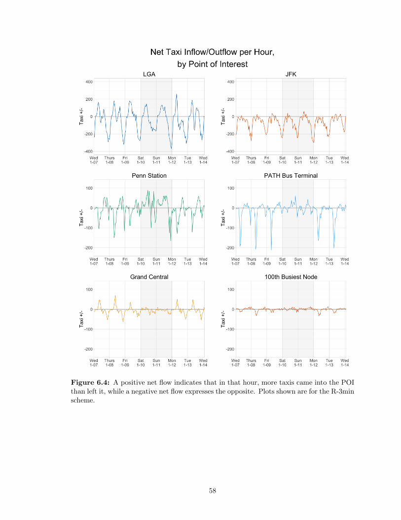
Figure 6.4: A positive net flow indicates that in that hour, more taxis came into the POIthan left it, while a negative net flow expresses the opposite. Plots shown are for the R-3minscheme.

58

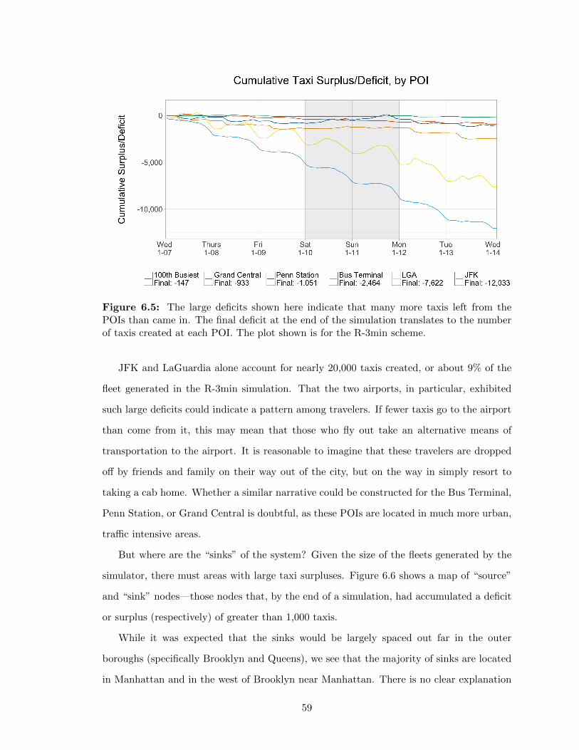
Figure 6.5: The large deficits shown here indicate that many more taxis left from thePOIs than came in. The final deficit at the end of the simulation translates to the numberof taxis created at each POI. The plot shown is for the R-3min scheme.

JFK and LaGuardia alone account for nearly 20,000 taxis created, or about 9% of the

fleet generated in the R-3min simulation. That the two airports, in particular, exhibited

such large deficits could indicate a pattern among travelers. If fewer taxis go to the airport

than come from it, this may mean that those who fly out take an alternative means of

transportation to the airport. It is reasonable to imagine that these travelers are dropped

off by friends and family on their way out of the city, but on the way in simply resort to

taking a cab home. Whether a similar narrative could be constructed for the Bus Terminal,

Penn Station, or Grand Central is doubtful, as these POIs are located in much more urban,

traffic intensive areas.

But where are the “sinks” of the system? Given the size of the fleets generated by the

simulator, there must areas with large taxi surpluses. Figure 6.6 shows a map of “source”

and “sink” nodes—those nodes that, by the end of a simulation, had accumulated a deficit

or surplus (respectively) of greater than 1,000 taxis.

While it was expected that the sinks would be largely spaced out far in the outer

boroughs (specifically Brooklyn and Queens), we see that the majority of sinks are located

in Manhattan and in the west of Brooklyn near Manhattan. There is no clear explanation

59

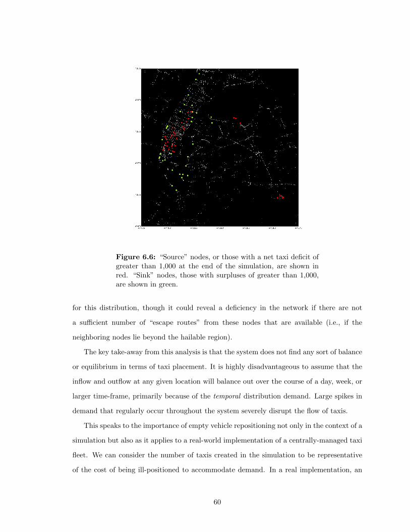
Figure 6.6: “Source” nodes, or those with a net taxi deficit ofgreater than 1,000 at the end of the simulation, are shown inred. “Sink” nodes, those with surpluses of greater than 1,000,are shown in green.

for this distribution, though it could reveal a deficiency in the network if there are not

a sufficient number of “escape routes” from these nodes that are available (i.e., if the

neighboring nodes lie beyond the hailable region).

The key take-away from this analysis is that the system does not find any sort of balance

or equilibrium in terms of taxi placement. It is highly disadvantageous to assume that the

inflow and outflow at any given location will balance out over the course of a day, week, or

larger time-frame, primarily because of the temporal distribution demand. Large spikes in

demand that regularly occur throughout the system severely disrupt the flow of taxis.

This speaks to the importance of empty vehicle repositioning not only in the context of a

simulation but also as it applies to a real-world implementation of a centrally-managed taxi

fleet. We can consider the number of taxis created in the simulation to be representative

of the cost of being ill-positioned to accommodate demand. In a real implementation, an

60

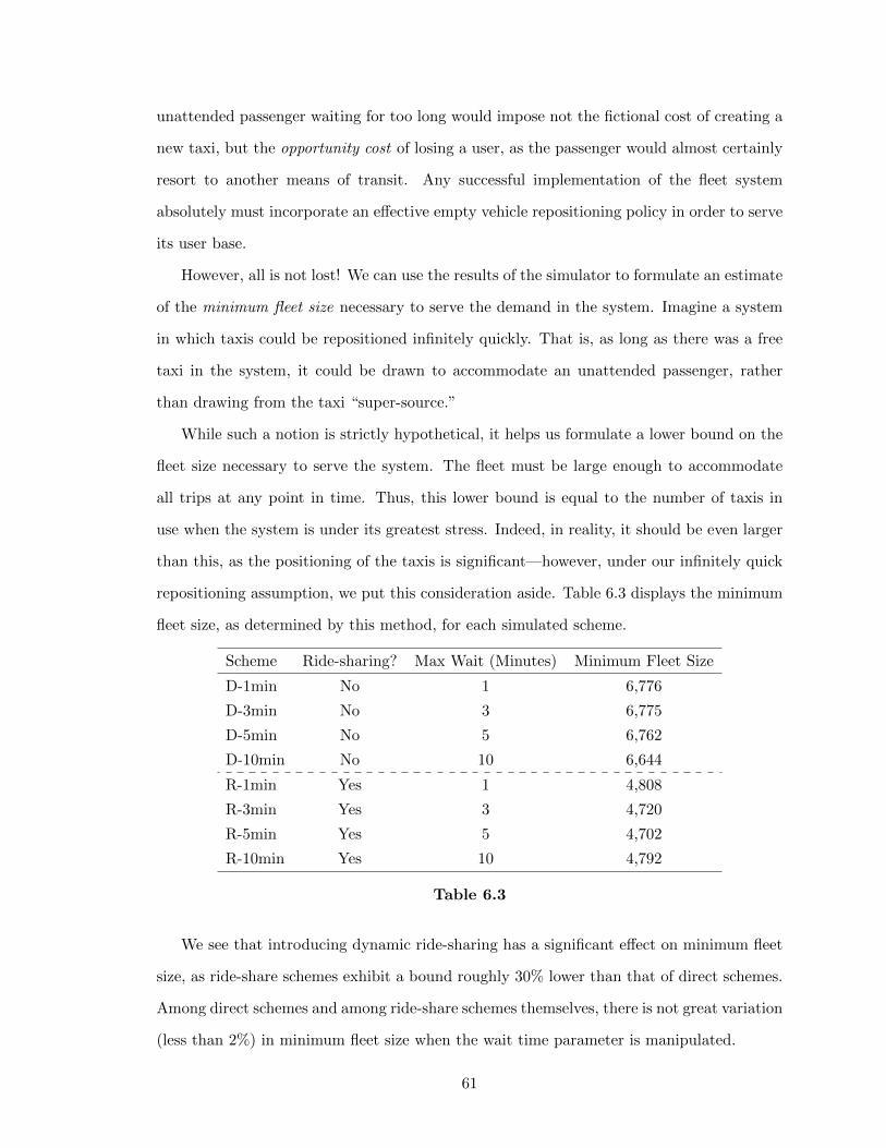
unattended passenger waiting for too long would impose not the fictional cost of creating a

new taxi, but the opportunity cost of losing a user, as the passenger would almost certainly

resort to another means of transit. Any successful implementation of the fleet system

absolutely must incorporate an effective empty vehicle repositioning policy in order to serve

its user base.

However, all is not lost! We can use the results of the simulator to formulate an estimate

of the minimum fleet size necessary to serve the demand in the system. Imagine a system

in which taxis could be repositioned infinitely quickly. That is, as long as there was a free

taxi in the system, it could be drawn to accommodate an unattended passenger, rather

than drawing from the taxi “super-source.”

While such a notion is strictly hypothetical, it helps us formulate a lower bound on the

fleet size necessary to serve the system. The fleet must be large enough to accommodate

all trips at any point in time. Thus, this lower bound is equal to the number of taxis in

use when the system is under its greatest stress. Indeed, in reality, it should be even larger

than this, as the positioning of the taxis is significant—however, under our infinitely quick

repositioning assumption, we put this consideration aside. Table 6.3 displays the minimum

fleet size, as determined by this method, for each simulated scheme.

Scheme Ride-sharing? Max Wait (Minutes) Minimum Fleet Size

D-1min No 1 6,776

D-3min No 3 6,775

D-5min No 5 6,762

D-10min No 10 6,644

R-1min Yes 1 4,808

R-3min Yes 3 4,720

R-5min Yes 5 4,702

R-10min Yes 10 4,792

Table 6.3

We see that introducing dynamic ride-sharing has a significant effect on minimum fleet

size, as ride-share schemes exhibit a bound roughly 30% lower than that of direct schemes.

Among direct schemes and among ride-share schemes themselves, there is not great variation

(less than 2%) in minimum fleet size when the wait time parameter is manipulated.

61

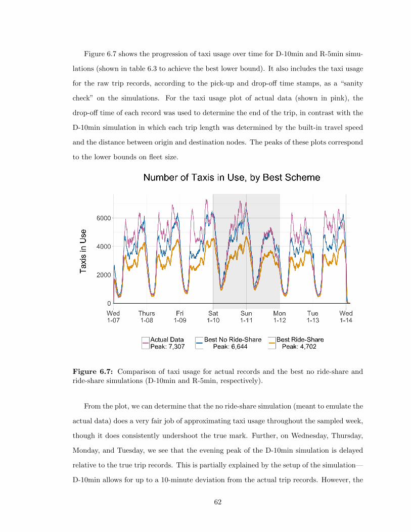
Figure 6.7 shows the progression of taxi usage over time for D-10min and R-5min simu-

lations (shown in table 6.3 to achieve the best lower bound). It also includes the taxi usage

for the raw trip records, according to the pick-up and drop-off time stamps, as a “sanity

check” on the simulations. For the taxi usage plot of actual data (shown in pink), the

drop-off time of each record was used to determine the end of the trip, in contrast with the

D-10min simulation in which each trip length was determined by the built-in travel speed

and the distance between origin and destination nodes. The peaks of these plots correspond

to the lower bounds on fleet size.

Figure 6.7: Comparison of taxi usage for actual records and the best no ride-share andride-share simulations (D-10min and R-5min, respectively).

From the plot, we can determine that the no ride-share simulation (meant to emulate the

actual data) does a very fair job of approximating taxi usage throughout the sampled week,

though it does consistently undershoot the true mark. Further, on Wednesday, Thursday,

Monday, and Tuesday, we see that the evening peak of the D-10min simulation is delayed

relative to the true trip records. This is partially explained by the setup of the simulation—

D-10min allows for up to a 10-minute deviation from the actual trip records. However, the

62

time difference in these peaks appears to be greater than this small margin. While the

cause of this remains unclear, it is possible that the simulation is overestimating the travel

time required to complete the trips—that is, the travel speed built into the simulator (11.5

mph) is too low.

With these limitations in mind, we can assess from the plot that the ride-sharing scheme

consistently exhibits significantly lower taxi usage than both the no ride-sharing scheme

and the true records during the day, though at times of low demand there is not a notable

difference.

6.3 Summary

The collection of simulation data presented above poses a strong argument supporting

the merits of dynamic ride-sharing. Ride-sharing schemes consistently and significantly

outperformed non-ride-sharing schemes in all relevant metrics—vehicle miles, AVO, and fleet

size (or, minimum fleet size). However, this examination of the data was also valuable for

the insights it provided into the simulator’s quirks—both its strengths and its shortcomings.

The following chapter provides a formal discussion of the limitations of these findings, and

presents the next steps.

63

Chapter 7

Limitations, Next Steps, and

Conclusion

7.1 Limitations

7.1.1 Limited Dataset

A key factor of this study—distinguishing it from many other ride-sharing studies—was its

use of real trip data. The New York TLC trip records proved truly invaluable for conducting

the analysis. They drastically reduced the number of assumptions made, and formed a firm

base upon which to judge results. Further, the number of available records is abundant—

data of precision identical to the records used in this study are available dating back to

January 2009. However, due to computational limitations, the simulation was conducted

over just one week of TLC trips.

While this study made a deliberate effort to choose a time frame representative of the

“average” week of trips, a more extensive study would span a larger time frame. This would

not only offer the opportunity to solidify results by sampling a larger number of trips—it

would also provide a natural “stress test” for the simulation. As described in Section

5.1, there existed several days during 2015 which exhibited significant spikes and drops in

demand. An effective implementation of a centrally-managed taxi fleet should certainly be

required to appropriately address each of these situations.

64

The study was also limited by its restriction to yellow-cab trip data. Ideally, data from

Uber and Lyft— which have grown to become significant players in the New York City

transportation scheme—would be utilized as well. The addition of this data would add

geographic diversity to the trip records. Each firm has claimed that it serves the outer

boroughs of the city better than the TLC taxis do. Thus, data from these services would

help illuminate the “dark regions” of New York pictured in Figure 5.4 that are not well

represented in the TLC records.

7.1.2 Network Detail

Another differentiating factor of the study was its choice to use a map network to serve as the

underlying basis for simulation rather than resort to pixelization. The map network acquired

from ALK Technologies is fairly comprehensive and proved very easy to use. However, it

does have its defects in the context of this study.

As we saw in Chapter 5, the spacing of the nodes could play a critical role in how the

trip origin and destination coordinates are mapped to the network. While the network

used here certainly achieves a broad characterization of the streets and intersections in the

city, in some regions (e.g. West Village) it lacks the high definition that would be ideal for

conducting a rigorous study.

7.1.3 Taxi Creation Dynamics

A limitation of the simulation examined extensively in Chapter 6 was the process by which

taxis were created. The simulator initializes the system with zero taxis, and gradually

construct the fleet by creating taxis, or pulling them from a “super-source” when necessary,

assuming that this process would gradually lead the system to a fleet size equilibrium.

What was not anticipated, however, was that the temporal and spatial distributions

would evolve such that no equilibrium could be reached—the system, quite simply, does

not balance itself out. This mistaken assumption cost the simulation greatly in terms of

estimating fleet size, as the number of taxis created ballooned, and the rate at which they

were created showed no signs of slowing even at the end of the simulation.

An alternative approach would be to fix the number of taxis at the real TLC fleet size,

65

and then simply summon the closest available taxi for any unattended passengers waiting

longer than the maximum wait time. Alternatively, and preferably, we could implement an

effective empty vehicle repositioning scheme (see Section 7.2.1).

7.1.4 Simulation Assumptions

As with any study, this thesis is limited by the assumptions and approximations it made.

One such assumption made in the simulation was the vehicle travel speed, which was set to

a constant 11.5 miles per hour throughout the simulated week. Of course, the true travel

speed of a taxi varies both with the time of day and with its geographic location. The speed

of a taxi on FDR Drive in the late evening is certainly higher than it is in Midtown during

rush hour.

Another assumption that was made was passengers’ indifference to time inconvenience.

The simulation had no restrictions on the number of trips that a passenger could be forced

to share during his or her own journey. For example, a taxi was permitted to pick up a

first passenger A, make a detour to pick up a second passenger B, drop off B, and pick up

a third passenger C before eventually dropping off passenger A—all as long as the itinerary

saved vehicle miles. In a realistic application of dynamic ride-sharing, this situation would

be avoided for the time burden it places on the first passenger. Indeed, Uber Pool and

Lyft Line both currently assure users that they will at most take one detour to pick-up

another passenger. Similarly, the simulation did not consider any directional inconvenience

its ride-sharing matches may have caused. In reality, a rider whose taxi turns around to

pick up another passenger nearby may grow disgruntled—psychologically, turning around

and retracing steps is hard to justify.

While these assumptions limited how realistic the simulation could be, the restriction

on the number of passengers a taxi could accommodate certainly limited the academically

motivated side of this thesis. Removing this bound would likely open the door for taxis

with many more passengers, especially those leaving points of interest with high origination

volumes. This would provide additional insight into the type of vehicles that the fleet could

offer—whether it should be expanded to include large shuttle vans or even buses. However,

due to computational limitations, the capacity of each taxi was capped at two.

66

7.2 Next Steps

7.2.1 Empty Vehicle Repositioning

As discussed in Chapter 6 and in the previous section, this study was handicapped by its

exclusion of an effective empty vehicle repositioning policy. Thus, I take this opportunity

to emphasize that, empty vehicle repositioning is the key next step to the development

of a comprehensive simulator, and in turn, the judgement of the ride-sharing potential of a

system.

A few simply heuristics could be considered. First, the simulation could be drastically

improved if we determined and outlined the low activity areas of the system. From here,

we could specify that any taxis terminating in these areas would be directed to relocate to

the nearest high activity point of interest (e.g. LaGuardia or JFK, or even a lower scale,

more local POI). Then, we could reasonably mandate that passengers in these low activity

endure a longer wait time, thus expanding and extending the search for a match. This

would drastically reduce the number of taxis required to serve the system.

Alternatively, using the large trove of TLC data to our advantage, we could conduct

a focused study on the spatial and temporal distribution of trips throughout the system.

From here, we could create prediction targets for demand at each point on the network

throughout the day. As shown in Chapter 5, the records do exhibit noticeable patterns

that could be exploited, especially at the high activity POIs that were studied. Further,

the scope of the records available ensure that we could track how demand evolves not only

over the course of the week (weekday vs. weekend travel), but also over the course of the

year (winter vs. summer). Taxis could then be relocated according to these patterns and

predictions.

7.2.2 Passenger Convenience Tuning

In order to achieve the transportation revolution described in the Introduction, we can

imagine that a fleet managing firm would have to reach a critical mass of trip demand. In

an age driven by consumer experience with plenty of competition and alternatives for users

to choose from, it is likely that only a firm that put the considerations of its passengers first

67

would be able to grow to this size.

I describe in the previous section how passenger preferences were somewhat disregarded

in pursuit of ride-sharing potential. This thesis took a rather theoretical approach, but

a study directed at explicitly proving the viability of a centrally managed dynamic ride-

sharing fleet would have to show that the benefits of ride-sharing hold even when passengers

are afforded a generous level of comfort and convenience.

Most significantly, we could limit ride-share matches to just one per passenger—that

is, no passenger would have to make more than one detour during his or her trip to pick

up another passenger. This very reasonable restriction would likely curb the number of

trips shared and the number of vehicle miles saved. Further, we could impose a restriction

that ride-share matches only be made when the vehicle miles saved exceeds some threshold.

Currently, the simulation eagerly matches any two passengers so long as there is any mileage

to be saved from doing so. However, we may decide that saving a few miles is not worth

inconveniencing either passenger.

7.3 Closing Remarks

In a growing number of social and political spheres, the finiteness of the resources on our

planet is being recognized as the most critical issue we face today. The matter is as scientific

and economic as it is ethical and existential. While engineering advancements are made

every day, improving the efficiency of our engines and reducing our waste production, the

reality remains that in order to achieve energy sustainability, we must fundamentally change

the way we consume resources. On the transportation front, we are on the precipice of this

very paradigm shift.

That ride-sharing will some day become a part of our transportation paradigm is ir-

refutable. The efficiencies that it offers are too great to ignore, and the opportunity cost

of resisting a shift is growing. Our primary motivation for the shift should be the ensured

reduction in the use of natural resources at all stages of the transportation cycle—those

that go into making the vehicles, those that fuel them, and those that absorb their byprod-

ucts. But even if this is not sufficient, market forces will eventually be forced recognize the

68

economies that ride-sharing has to offer.

It begins with the significantly reduced mileage and a minimal fleet size necessary to

accommodate demand. These savings for the fleet manager are be passed on to passengers,

offering a drastically more cost efficient mode of transportation. Further, a well-managed

fleet would serve to dramatically reduce road congestion, making transit quicker and more

painless. This vision of a centrally managed ride-sharing-optimized service is one that is

cost-effective, efficient, and sustainable. And, most importantly, the results of this study

strengthen the argument that it is achievable.

This thesis set out to examine the ride-sharing potential of one of the busiest transporta-

tion systems in the world. It sought to impose stricter constraints than models implemented

in previous studies, restricting motion to a map network and using actual trip records to

try and emulate observable travel patterns. Offsetting these restrictions, it permitted more

flexible rules for ride-sharing, opting for a dynamic ride-sharing policy that continuously

matches passengers “on the go.” The result, I believe, is a fairly realistic model of the

ride-sharing dynamics at play in the system.

The numerical results of this study are promising, with dynamic ride-sharing schemes

using a smaller fleet and drastically fewer vehicle miles to accommodate the same demand

as the present non-ride-sharing scheme. It is my hope that this study will contribute to the

greater body of academic work that will ultimately bring ride-sharing and its benefits to

fruition.

69

Bibliography

Agatz, N. (2010). The Value of Optimization in Dynamic Ride-Sharing: A Simulation

Study in Metro Atlanta. ERIM report series research in management. Erasmus Research

Institute of Management, Erasmus University.

Brownell, C. and Kornhauser, A. (2014). A driverless alternative: Fleet size and cost

requirements for a statewide autonomous taxi network in new jersey. Transportation

Research Record: Journal of the Transportation Research Board.

Cook, J. Uber’s internal charts show how its driver-rating system actually works.

Douglas, K. (2015). Truly empty vehicle repositioning and fleet-sizing: Optimal manage-

ment of an autonomous taxi system in new jersey on a typical weekday.

Mosendz, P. and Sender, H. Here’s how long it takes to get an uber in us cities.

Sivak, M. Hitchin’ a ride: Fewer americans have their own vehicle.

Song, D.-P. and Earl, C. F. (2008). Optimal empty vehicle repositioning and fleet-sizing for

two-depot service systems. European Journal of Operational Research.

Stiles, R. (2014). 2014 taxicab factbook. New York City Taxi & Limousine Commission

Office of Policy and External Affairs.

Swoboda, A. J. (2015). New york city taxicab transportation demand modeling for the

analysis of ridesharing and autonomous taxi systems.

Tangel, A. Uber logs major gains in new york city, figures show.

Wellington, B. (2014). Quantifying the best and worst times of day to hit the road in nyc.

70