Embed Size (px)
Citation preview

Quantitative Methods for Data DrivenReliability Optimization of Engineered Systems
Dissertationzur Erlangung des Grades eines Doktors der Naturwissenschaften
an der Fakultät für Mathematik, Informatik und Statistikder Ludwig-Maximilians-Universität München
vorgelegt/eingereicht von
Lukas Felsberger
29.10.2020


Erstgutachter: Prof. Dr. Dieter Kranzlmüller
Zweitgutachter: Prof. Dr. Rüdiger Schmidt
Tag der mündlichen Prüfung: 25.01.2021

Eidesstattliche Versicherung(Siehe Promotionsordnung vom 12.07.11, § 8, Abs. 2 Pkt. .5.)
Hiermit erkläre ich an Eidesstatt, dass die Dissertation von mir selbstständig, ohne unerlaubteBeihilfe angefertigt ist.
Genf, am 29.10.2020 . . . . . . . . . . . . . . . . . . . . . . . . . . . . . . . . . . . . . . . . . . . .Lukas Felsberger

Acknowledgements
In retrospect, the recent years taught me the ability to see my work, myself, and othersfrom new and valuable perspectives. I am convinced that this will have a lasting, positiveeffect on my future career and personal development. This has only been possible due topeople to whom I would like to express my sincere gratitude.
Prof. Dr. Dieter Kranzlmüller, for his supervision of my thesis at the Ludwig-Maximilians-Universität München and for providing the right questions and answers at the right timefrom the very first moment on.
Prof. Dr. Rüdiger Schmidt, for his immediate availability to review my thesis, hisdetailed and thought-through comments, and inspiring discussions.
Dr. Benjamin Todd, for giving me freedom to pursue my goals, the necessary sup-port whenever needed, and defending my interests when required. Yours was the greatestcontribution in making these three years a rewarding and interesting journey.
Prof. Andreas Müller, for inspiring discussions and determined support even beyondoffice hours.
Jan Uythoven and Andrea Apollonio, for fruitful collaborations in the Reliability andAvailability Studies Working Group.
My colleagues, David Nisbet, Yves Thurel, Slawosz Uznanski, Thomas Cartier-Michaud,Volker Schramm, Arto Niemi, Jochen Schwenk, Christophe Martin, Raul Murillo Garcia,Konstantinos Papastigerou, and the whole CCE section, for sharing their expertise andopinion, which helped me developing my ideas and approaches further, in a productive yetfriendly atmosphere.
The German Doctoral Student Programme, the Future Circular Collider Study atCERN, for offering and funding this interesting research project and the TE-EPC groupled by Jean Paul Burnet for hosting my research in a compelling environment.
Finally, I want to express my gratitude to my parents and sister for giving me confidencein myself even if I had utterly failed in this ambitious project. In short, thank you forremembering me of the many important things outside a PhD cosmos. Thanks to myawesome friends for making the outside PhD cosmos as fun and as exciting as it can be.

vi

Abstract
Particle accelerators, such as the Large Hadron Collider at CERN, are among the largestand most complex engineered systems to date. Future generations of particle acceleratorsare expected to increase in size, complexity, and cost. Among the many obstacles, thisintroduces unprecedented reliability challenges and requires new reliability optimizationapproaches.
With the increasing level of digitalization of technical infrastructures, the rate andgranularity of operational data collection is rapidly growing. These data contain valuableinformation for system reliability optimization, which can be extracted and processed withdata-science methods and algorithms. However, many existing data-driven reliability opti-mization methods fail to exploit these data, because they make too simplistic assumptionsof the system behavior, do not consider organizational contexts for cost-effectiveness, andbuild on specific monitoring data, which are too expensive to record.
To address these limitations in realistic scenarios, a tailored methodology based onCRISP-DM (CRoss-Industry Standard Process for Data Mining) is proposed to developdata-driven reliability optimization methods. For three realistic scenarios, the developedmethods use the available operational data to learn interpretable or explainable failuremodels that allow to derive permanent and generally applicable reliability improvements:Firstly, novel explainable deep learning methods predict future alarms accurately from fewlogged alarm examples and support root-cause identification. Secondly, novel parametricreliability models allow to include expert knowledge for an improved quantification offailure behavior for a fleet of systems with heterogeneous operating conditions and deriveoptimal operational strategies for novel usage scenarios. Thirdly, Bayesian models trainedon data from a range of comparable systems predict field reliability accurately and revealnon-technical factors’ influence on reliability.
An evaluation of the methods applied to the three scenarios confirms that the tai-lored CRISP-DM methodology advances the state-of-the-art in data-driven reliability op-timization to overcome many existing limitations. However, the quality of the collectedoperational data remains crucial for the success of such approaches. Hence, adaptations ofroutine data collection procedures are suggested to enhance data quality and to increase thesuccess rate of reliability optimization projects. With the developed methods and findings,future generations of particle accelerators can be constructed and operated cost-effectively,ensuring high levels of reliability despite growing system complexity.

viii

Zusammenfassung
Teilchenbeschleuniger, wie z.B. der Large Hadron Collider am CERN, gehören zu den bishergrößten und komplexesten technischen Systemen. Es wird erwartet, dass zukünftige Gener-ationen von Teilchenbeschleunigern an Größe, Komplexität und Kosten zunehmen werden.Unter den vielen Hindernissen führt dies zu noch nie dagewesenen Herausforderungen andie Zuverlässigkeit und erfordert neue Ansätze zur Zuverlässigkeitsoptimierung.
Mit der zunehmenden Digitalisierung nimmt die Geschwindigkeit und Granularitätder Betriebsdatenerfassung rasch zu. Diese Daten enthalten wertvolle Informationen fürdie Optimierung der Systemzuverlässigkeit, die mit datenwissenschaftlichen Methoden ex-trahiert werden können. Viele existierende datenbasierte Zuverlässigkeitsoptimierungsmeth-oden nutzen diese Möglichkeit nur unzureichend aus, weil sie zu vereinfachende Annahmenüber das Systemverhalten treffen, organisatorische Kontexte für die Kosteneffizienz nichtberücksichtigen und auf spezifischen Betriebsdaten aufbauen, deren Erfassung zu teuer ist.
Um diese Einschränkungen in realistischen Szenarien zu überwinden, wird eine maßgeschnei-derte Methodik vorgeschlagen, die auf CRISP-DM (CRoss-Industry Standard Process forData Mining) basiert, um datenbasierte Zuverlässigkeitsoptimierungsmethoden zu entwick-eln. Für drei realistische Szenarien nutzen die entwickelten Methoden die verfügbarenBetriebsdaten, um interpretierbare Versagensmodelle zu erlernen, die es erlauben, dauer-hafte und allgemein anwendbare Zuverlässigkeitsverbesserungen abzuleiten: (1) Neuartigeerklärbare Deep-Learning Methoden sagen zukünftige Alarme aus wenigen protokolliertenAlarmbeispielen genau voraus und unterstützen die Ursachenermittlung. (2) Neuartigeparametrische Zuverlässigkeitsmodelle erlauben die Einbeziehung von Expertenwissen füreine verbesserte Quantifizierung des Ausfallverhaltens für eine Flotte von Systemen mit het-erogenen Betriebsbedingungen und die Ableitung optimaler Betriebsstrategien für neuar-tige Nutzungsszenarien. (3) Bayes’sche Modelle, die mit Daten aus einer Reihe vergleich-barer Systeme trainiert wurden, sagen die Zuverlässigkeit genau voraus und zeigen denEinfluss nicht-technischer Faktoren auf die Zuverlässigkeit auf.
Eine Bewertung der angewandten Methoden bestätigt, dass die maßgeschneiderte CRISP-DM-Methodik viele bestehende Einschränkungen überwindet. Die Qualität der gesam-melten Betriebsdaten bleibt jedoch entscheidend für den Erfolg solcher Ansätze. Daherwerden Anpassungen der routinemäßigen Datenerfassungsverfahren vorgeschlagen, um dieDatenqualität zu verbessern und die Erfolgsrate von Zuverlässigkeitsoptimierungsprojek-ten zu erhöhen. Mit den entwickelten Methoden und Erkenntnissen kann kostengünstig einhohes Maß an Zuverlässigkeit für zukünftige Teilchenbeschleuniger gewährleistet werden.

x

Contents
Acknowledgements v
Abstract vi
1 Introduction 11.1 Motivation . . . . . . . . . . . . . . . . . . . . . . . . . . . . . . . . . . . . 11.2 Research Questions, Objectives and Contributions . . . . . . . . . . . . . . 6
1.2.1 Current Limitations . . . . . . . . . . . . . . . . . . . . . . . . . . 61.2.2 Research Questions . . . . . . . . . . . . . . . . . . . . . . . . . . . 7
1.3 List of Peer-Reviewed Publications and Declaration of Authorship . . . . . 111.4 Structure of the Thesis . . . . . . . . . . . . . . . . . . . . . . . . . . . . . 12
2 Particle Accelerators 132.1 Introduction to Particle Accelerators . . . . . . . . . . . . . . . . . . . . . 132.2 CERN . . . . . . . . . . . . . . . . . . . . . . . . . . . . . . . . . . . . . . 14
2.2.1 LHC . . . . . . . . . . . . . . . . . . . . . . . . . . . . . . . . . . . 142.2.2 PSB . . . . . . . . . . . . . . . . . . . . . . . . . . . . . . . . . . . 162.2.3 FCC . . . . . . . . . . . . . . . . . . . . . . . . . . . . . . . . . . . 16
2.3 Existing and Future Reliability Challenges for Particle Accelerators . . . . 172.4 Magnet Power Converters . . . . . . . . . . . . . . . . . . . . . . . . . . . 18
3 Backgrounds 213.1 Reliability Engineering . . . . . . . . . . . . . . . . . . . . . . . . . . . . . 213.2 Data, Information and Knowledge . . . . . . . . . . . . . . . . . . . . . . . 313.3 Artificial Intelligence and Machine Learning . . . . . . . . . . . . . . . . . 32
4 Literature Review 414.1 Literature Overview . . . . . . . . . . . . . . . . . . . . . . . . . . . . . . 414.2 Existing Limitations of Data-Driven Frameworks for Reliability Optimization 42
5 Methodology 475.1 Overview . . . . . . . . . . . . . . . . . . . . . . . . . . . . . . . . . . . . . 475.2 Constructive Methodology . . . . . . . . . . . . . . . . . . . . . . . . . . . 47
5.2.1 Project Assessment . . . . . . . . . . . . . . . . . . . . . . . . . . . 48
xii CONTENTS
5.2.2 Project Implementation . . . . . . . . . . . . . . . . . . . . . . . . 505.2.3 Limitations of the Constructive Methodology . . . . . . . . . . . . . 515.2.4 Structure of Constructive Chapters . . . . . . . . . . . . . . . . . . 52
5.3 Evaluative Methodology . . . . . . . . . . . . . . . . . . . . . . . . . . . . 535.3.1 Limitations of the Evaluative Methodology . . . . . . . . . . . . . . 53
6 Data-Driven Discovery of Failure Mechanisms 556.1 Scenario Description and Problem Definition . . . . . . . . . . . . . . . . . 556.2 Related Work and Method Selection . . . . . . . . . . . . . . . . . . . . . 566.3 Methodology - Explainable Deep Learning Models for Failure Mechanism
Discovery . . . . . . . . . . . . . . . . . . . . . . . . . . . . . . . . . . . . 606.3.1 Pseudoalgorithm . . . . . . . . . . . . . . . . . . . . . . . . . . . . 65
6.4 Data Requirements and Availability . . . . . . . . . . . . . . . . . . . . . . 666.5 Numerical Experiments . . . . . . . . . . . . . . . . . . . . . . . . . . . . . 68
6.5.1 Synthetic Data Experiments . . . . . . . . . . . . . . . . . . . . . . 686.5.2 Particle Accelerator Data Experiments . . . . . . . . . . . . . . . . 726.5.3 Further applications . . . . . . . . . . . . . . . . . . . . . . . . . . 76
6.6 Chapter Summary, Conclusions and Outlook . . . . . . . . . . . . . . . . . 77
7 Data and Knowledge-Driven Parametric Model-Based Reliability Opti-mization 797.1 Scenario Description and Problem Definition . . . . . . . . . . . . . . . . . 807.2 Related Work and Methods Selection . . . . . . . . . . . . . . . . . . . . . 817.3 Methodology - Parametric Digital Reliability Twins . . . . . . . . . . . . . 83
7.3.1 Overview . . . . . . . . . . . . . . . . . . . . . . . . . . . . . . . . 837.3.2 Reliability Modeling of Load Sharing in Redundant Systems . . . . 847.3.3 Simulation Engine . . . . . . . . . . . . . . . . . . . . . . . . . . . 887.3.4 Cost Model . . . . . . . . . . . . . . . . . . . . . . . . . . . . . . . 907.3.5 Data Requirements and Availability . . . . . . . . . . . . . . . . . . 91
7.4 Numerical Experiments . . . . . . . . . . . . . . . . . . . . . . . . . . . . . 927.4.1 Further Applications . . . . . . . . . . . . . . . . . . . . . . . . . . 96
7.5 Chapter Summary, Conclusions and Outlook . . . . . . . . . . . . . . . . . 97
8 Data-Driven Discovery of Organizational Reliability Aspects 998.1 Scenario Description and Problem Definition . . . . . . . . . . . . . . . . . 998.2 Related Work and Methods Selection . . . . . . . . . . . . . . . . . . . . . 1018.3 Methodology - Statistical System Life Cycle Models . . . . . . . . . . . . . 102
8.3.1 Definitions . . . . . . . . . . . . . . . . . . . . . . . . . . . . . . . . 1028.3.2 Approach . . . . . . . . . . . . . . . . . . . . . . . . . . . . . . . . 1038.3.3 Model Selection and Validation . . . . . . . . . . . . . . . . . . . . 105
8.4 Numerical Experiments . . . . . . . . . . . . . . . . . . . . . . . . . . . . . 1088.4.1 Data Requirements and Availability . . . . . . . . . . . . . . . . . . 1088.4.2 Model Selection and Validation . . . . . . . . . . . . . . . . . . . . 110

Table of Contents xiii
8.4.3 Prediction . . . . . . . . . . . . . . . . . . . . . . . . . . . . . . . . 1168.4.4 Discussion . . . . . . . . . . . . . . . . . . . . . . . . . . . . . . . . 116
8.5 Chapter Summary, Conclusions and Outlook . . . . . . . . . . . . . . . . . 119
9 Synthesis: Developing Robust Data-Driven Reliability Optimization Meth-ods 1219.1 Critical Assessment of Constructive Chapters . . . . . . . . . . . . . . . . 122
9.1.1 Addressing Practical Limitations . . . . . . . . . . . . . . . . . . . 1229.1.2 Usefulness of the Tailored CRISP-DM Methodology . . . . . . . . . 125
9.2 Embedding Data-Driven Reliability Optimization Methods in System LifeCycles . . . . . . . . . . . . . . . . . . . . . . . . . . . . . . . . . . . . . . 1289.2.1 Embedding Data-Driven Discovery of Failure Mechanisms . . . . . 1289.2.2 Embedding Data and Knowledge-Driven Parametric Model-Based
Reliability Optimization . . . . . . . . . . . . . . . . . . . . . . . . 1299.2.3 Embedding Data-Driven Discovery of Organizational Reliability As-
pects . . . . . . . . . . . . . . . . . . . . . . . . . . . . . . . . . . . 1309.2.4 Using the Methods for Cost-Effective Decision Making . . . . . . . 131
9.3 Improving Data Quality through Automatic Reliability Data Collection . . 1319.3.1 Types of Data Required for Reliability Optimization . . . . . . . . 1329.3.2 Design for Automatic Reliability Collection . . . . . . . . . . . . . . 1339.3.3 Organization for Automatic Reliability Data Collection . . . . . . . 134
9.4 A Data-Driven Framework for Cost-Effective Continuous Reliability Opti-mization . . . . . . . . . . . . . . . . . . . . . . . . . . . . . . . . . . . . . 135
10 Conclusions and Future Research Directions 13710.1 Future Research Directions . . . . . . . . . . . . . . . . . . . . . . . . . . . 139

xiv Table of Contents

Chapter 1
Introduction
1.1 Motivation
CERN, High Energy Particle Accelerators and Future Challenges Particle ac-celerators study the fundamental constituents of matter as well as the laws which governtheir interaction. The Large Hadron Collider (LHC) at the European Organization forNuclear Research (CERN) has significantly advanced human understanding of matter byprobing it at unprecedented particle collision energies of up to 14 TeV. Most notably, theHiggs Boson was discovered in 2012. It was the last missing particle of the Standard Modelof particle physics, which describes most of the known universe. Yet, open questions aboutthe behavior of the unknown universe remain. These include dark matter, the asymmetryof matter and antimatter, and neutrino masses.[1]
Particle accelerators with even higher collision energies promise to shine a light on theseunresolved mysteries. Few organizations have the capabilities and experience to build suchaccelerators. The Future Circular Collider (FCC) study has been initiated to study optionsfor future accelerators at the high-energy frontier at CERN. A new 80-100 km tunnel isproposed to house particle accelerators with collision energies of up to 100 TeV.[2, 3]
The operation of the LHC poses many challenges due to its complexity, its highlyspecialized sub-systems which are produced in low volumes, as well as the geographicalexpand of its infrastructure around the 27 km accelerator tunnel. The stored beam energyas well as the magnetic energy in the superconducting magnetic circuits posed novel risksfor particle accelerators. New accelerators with circumferences of 100 kms and energieseight times higher than LHC are expected to set unprecedented requirements for their safeand reliable operation.
This thesis aims to develop quantitative, data-driven methods to optimize the reliabilityof particle accelerators and their sub-systems. A particular focus for the practical validationof the methods is put on power converters. They process and control the flow of electricalenergy by supplying voltages and currents in a form that is optimally suited for electricalloads [4]. Particle accelerators consume electrical energy for their operation and containvarious types of electrical loads. Among them, the powering of magnetic circuits and radio-

2 1. Introduction
frequency systems can represent up to 70-90% of the energy consumption [5]. As powerconverters are numerous and essential for operation, they impact the overall reliability ofa particle accelerator significantly. Hence, they are chosen as representative sub-system tovalidate the developed methods, which can be applied to other systems as well.
The developed methods should help to improve the reliability of particle acceleratorsub-systems despite their complexity growth at moderate additional investments to meetperformance, reliability, and cost targets that make future particle accelerators projectsfeasible.
Reliability People, organizations and society have adopted engineered systems thatfunction reliably. Systems that fail to function as expected have either not been adoptedor abandoned quickly. Systems we use every day, such as doors, elevators, or cars, oftenonly receive our attention when they fail to work. We have become used to them becausethey carry out their function or purpose as we expect it. Reliability is the ability of aproduct or system to perform as intended for a specified time, in its life cycle conditions[6].
In the widest sense, a system is a group of interacting entities that form a whole. Itis enclosed by a boundary and surrounded by an environment through which it interactsthrough inputs and outputs. In engineering settings, a system is an aggregation of elementsorganized to fulfill one or several stated purposes [7]. System specifications should includeits intended purposes and the conditions in which it needs to achieve them. A failureoccurs when a system stops achieving its purpose despite being operated according toits specifications. E.g., a system failing during an earthquake is denoted "reliable" whenits specifications exclude earthquakes as tolerable operating conditions. However, it isconsidered "unreliable" when it is supposed to withstand earthquakes.
Unreliability of an engineered system can principally be traced back to human activity.It may be the designer specifying wrong tolerances, the producer not manufacturing withincorrect tolerances, the user not operating in specified environments, or the managementnot providing the means and strategies to achieve the targeted reliability. This suggeststhat systems that always work as specified (i.e. 100% reliable) can be created in principle.However, even if all project stakeholders pay care to reliability aspects, systems can fail dueto the practically unforeseeable complexity of failure mechanisms and variation inherent innatural and human processes. Hence, being able to trace back a failure to a human activityshould not be confused with blaming system unreliability to human error. Instead, systemsshould be designed robustly to function reliably despite the possibility of human errors andunexpected environmental impacts. Then, systems can approach close to 100% reliabilityin practice [8].
Failures in systems, such as transportation, can compromise the safety of people. Fail-ures in production systems, e.g. in the semiconductor industry, can cause multi-millionlosses due to the interruption of a global supply chain. These are direct financial conse-quences of failure. However, failures also cause indirect financial consequences, such asloss of consumer trust, which leads to reduced revenue in the future. Therefore, many

1.1 Motivation 3
successful organizations have identified reliability as a key enabler of long-term success.Reliability Engineering is the technical discipline which aims to increase the relia-
bility of systems. Its goals in order of priority are
1. to prevent or to reduce the likelihood or frequency of failures,
2. to identify and correct the causes of failures, and
3. to determine ways of coping with failures that do occur.
The order reflects the expected effectiveness in terms of minimizing cost and increasingreliability [8].
Highly reliable systems are not achieved by reliability engineers but by a concertedeffort of designers, test engineers, manufacturers, suppliers, maintainers, and users. Therole of reliability engineers is to support such efforts by providing effective tools, specializedtraining, and data-driven insights.
Economics of Reliability and the System Life Cycle The system life cycle conceptincludes all phases of the existence of a system from its first idea to disposal or reuse. In thisthesis, the life cycle is separated in concept, design, production, field use and maintenance,and end-of-life phases.
It is generally observed that the cost to fix a problem rapidly increases until the pro-duction phase of the life cycle of a system as more and more project costs are committed.This is illustrated in Figure 1.1. It shows the cost to fix a problem (y axis) as a function ofthe life cycle phase (x axis). The rate of increase of the cost to fix a problem is particularlyhigh during the design and production phases.
Therefore, it is important to ensure a high system reliability as early as possible in thelife cycle. Failure to do so will result in change requests later in the life cycle with unnec-essarily high costs and project delays. To ensure reliability early in the life cycle, systemdesigners need to be able to make correct decisions. Therefore, reliability engineering ismost effective when it makes the necessary knowledge, tools, and data for decision makingavailable to system stakeholders as early as possible.
A common and established approach to achieve correct decision making in early lifecycle phases is to rely upon the knowledge of experienced project stakeholders. They gathertheir expertise in a structured way and used it to improve new systems early in their lifecycle. Such methods include Failure Mode and Effect Analysis (FMEA) [8], Fault TreeAnalysis (FTA) [6], and design review [9]. These methods are based on a manual analysisof the investigated systems. This manual approach is increasingly difficult for moderncomplex, interconnected, and adaptive systems.
Instead of relying on manual analysis, rapid advances in information technology, com-puter science, and electronics allow to observe the behavior of a system directly. Data-science algorithms can automatically learn models of system behavior and derive reliabilityoptimizations. Such improvements can help system stakeholders to follow up on the relia-bility of complex systems cost-effectively and improve their expertise.
4 1. Introduction
Figure 1.1: Cost of change in an engineering project throughout a system life cycle. [6]
This thesis presents a range of such methods to model system behavior, derive reliabilityimprovements, and provide insights to system experts to help them build better systemsin the future. In the following, the technological enablers of such data-driven approachesand their current limitations with respect to system reliability are discussed.
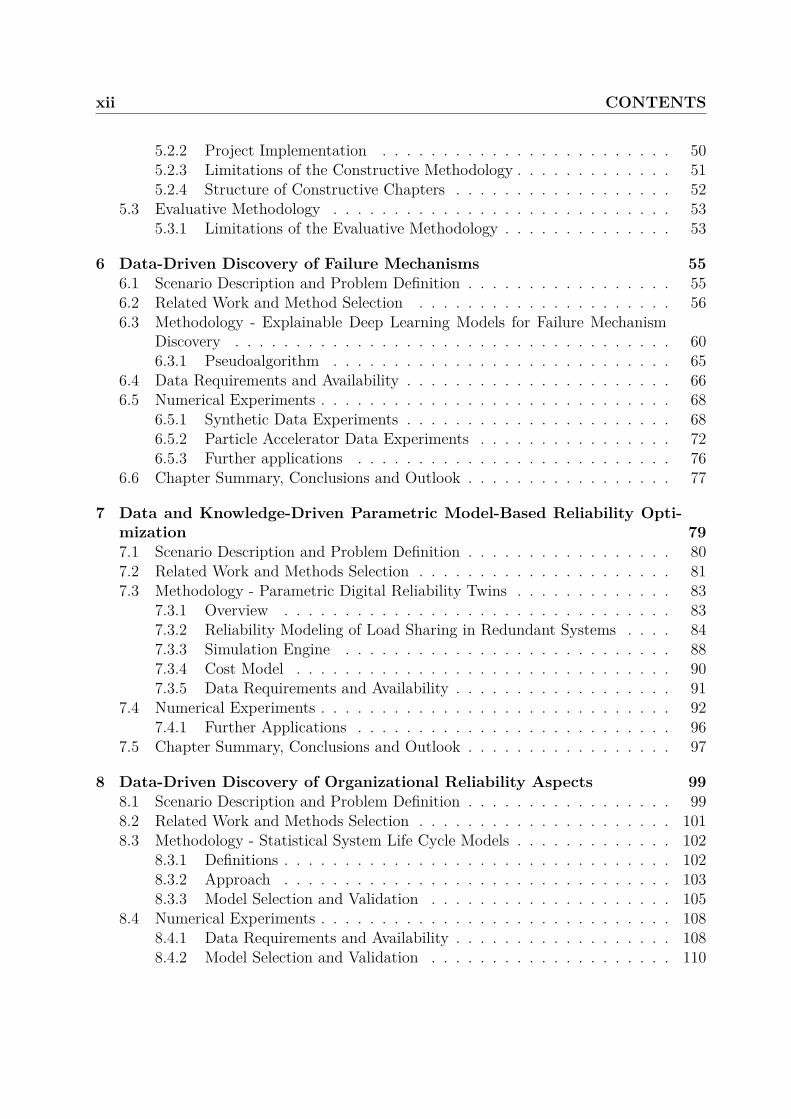
Digital Transformation Figure 1.2 shows the evolution of computing devices in termsof volume (red line and axis), price (blue line and axis), and number of installed devices(green line and axis) over the last decades (x axis). Their volume and price have decreasedby more than ten (!) orders of magnitude since the 1950s and as a result, the number of in-stalled computing devices has exploded. This has had a massive impact on the way people,organizations and societies function. The recent hardware, software, and methodologicaldevelopments are discussed with respect to their impact on system reliability:
• In terms of hardware, electronics and control systems have become ubiquitous inmodern machinery. More recently, an increased use of sensors makes systems avaluable source of data. Computing power has evolved with the growth of the datasize it needs to manipulate. In a few decades, systems have changed from simplemechanical apparatus to internet connected, communicating, adaptive and partiallyautonomous entities. This drastic change provides both opportunities and challengesfor system reliability, which are discussed below.With respect to the opportunities, system behavior and degradation can be mea-sured at unprecedented granularity through increased sensing capabilities at reducedcost. Remote diagnostics of machinery is possible due to instant worldwide datatransfer and communication. Advances in robotics promise autonomous or remotelycontrolled interventions in hazardous environments.Despite such improvements, there is a list of potential problems. Increased systemcomplexity bears more potential failure mechanisms. Equipping systems with sensors

1.1 Motivation 5
Figure 1.2: Evolution of computing devices over recent decades in terms of volume, price,and number of installed devices.
and computing capabilities increases their cost and energy consumption. Develop-ment and handling of machines that include mechanics, electronics, and software,demand an extended skill set from project stakeholders. Rapid technological changerequires continuous adaption and investment.
• In terms of software, so-called Industrial Internet of Things (IIoT) platforms provideintegrated frameworks of data collection, storage, visualization and analysis. Theyare offered by both commercial providers and as open source implementations [10].Often, existing organizational platforms can be extended to cater for increased datacollection and storage requirements. For data analysis and visualization, numeroussoftware packages have been introduced.Modern data analytics platforms allow monitoring, diagnosing and predicting systembehavior remotely and in real time. As for the introduction of electronics and sensinghardware, added software systems bear the risk of new system failure modes, increasesystem cost, and require project stakeholders to master additional skills.
• In terms of methodological advances, Artificial Intelligence (AI) and Machine Learn-ing (ML) are increasingly popular. Methods based on deep neural networks haveachieved or surpassed human performance in tasks such as image recognition or lan-guage translation [11]. Such methods benefit from a complex but versatile internalmodel structure and large data sets from which to detect patterns. In reliability en-gineering, problems are usually characterized by small data sets due to the scarcity

6 1. Introduction
of failures or anomalous behavior during operation and challenges in data collection.Furthermore, information is not just available in the form of quantified data but asexpert knowledge, which cannot easily be ’used’ by a neural network. Therefore, thebenefits of neural networks are not always fully exploitable in reliability problems.
Classical ML models include Random Forests [12], Naïve Bayes [13] and SupportVector Machines (SVMs) [14]. They achieve comparable performance to deep neuralnetworks for simple modeling tasks with small data sets at a fraction of the com-putational demand. Often they allow making use of expert knowledge as well asquantified data. However, deep neural networks generally outperform their modelingcapabilities on large complex data sets.
Bayesian probabilistic methods provide a systematic reasoning framework for limiteddata scenarios and quantify confidence in the parameters and predictions they pro-duce. However, their computational demand can exceed those of non-probabilisticmethods for the same tasks.
1.2 Research Questions, Objectives and Contributions
1.2.1 Current LimitationsWith the introduction of these novel technologies, maintenance optimization has becomea research trend within reliability studies. Manyika et al [15] estimated that such an op-timization has a global economic potential of 1.2 − 3.7 · 109 USD (as of 2015). Researchon monitoring, diagnosing and predicting system health has arguably received a lot ofattention in recent decades. The goal of such research is often to predict failures of sys-tems precisely in time. In comparison to the traditional approach of running machineryuntil breakdown, this promises to avoid unexpected system downtime. In comparison torigid time-scheduled preventive maintenance, a reduction of unnecessary interventions isexpected.
Such optimization methods can lead to increased system reliability and decreased costdespite the required capital investment for sensors, data handling infrastructure and im-plementation. Therefore, research has focused to monitor and predict system failure usinglatest technologies in sensing, data analysis, and ML. However, there are three frequentlimitations of such approaches.1
Firstly, many studies are carried out under laboratory conditions and are validatedon unrepresentative data sets, if at all [16]. Moreover, the algorithmic and mathematicalaspects are overemphasized, whereas, the required data collection and data quality, as wellas the embedding in organizational processes receive less attention [17, 18]. Therefore,success stories of data-driven reliability improvements in industrial settings remain rare[19].
1A more detailed treatment of limitations of existing approaches is provided in Section 4.2.

1.2 Research Questions, Objectives and Contributions 7
Secondly, existing approaches often rely on detailed condition monitoring of machinery.The required sensing equipment may be expensive and can introduce additional failuremodes. Given that the expected benefit is uncertain, many organizations do not wantto invest in additional condition monitoring systems [20, 21]. However, most systemsroutinely collect operational data through their control systems, which may indirectlyprovide reliability information [22, 23, 24]. Methods suited for such (sub-optimal) datascenarios are underrepresented in the literature.
Thirdly, studies aim to determine the correct timing of maintenance. However, suchstudies can also reveal findings that can be used to improve future systems at early lifecycle stages [21]. Referring to Figure 1.1, the potential cost benefit can be increased byorders of magnitude when insights lead to improved future system instead of optimizedmaintenance of existing systems. In other words, knowing when and how a system will failis not very valuable in comparison to knowing how to modify an existing system or designa future system so that such failures will not happen in the first place. Yet, the focus ofmany current methods remains solely on determining when systems are going to fail.
1.2.2 Research Questions
The previously mentioned limitations prevent a wider adoption of data-driven reliabilityoptimization methods despite their potential to improve the reliability of complex systemsat low cost and workforce investment.
Hence, the umbrella research question (Umbrella RQ) of this thesis asks how the afore-mentioned limitations can be resolved to develop robust data-driven system reliabilityoptimization methods from operational data and infer generally applicable strategies fordata-driven reliability optimization. It is addressed by proposing a general methodologyfor the development and implementation of reliability optimization methods, which hasthe potential to address the mentioned limitations of existing methods.
The proposed methodology is tested by executing it for the three representative reliabil-ity optimization use cases at CERN and evaluating whether it facilitates the developmentof data-driven methods that reach the state of the art performance or go beyond. Eachscenario is characterized by different optimization objectives, availability of data, and a pri-ori expert knowledge. Hence, they provide strong evidence towards the Umbrella RQ butalso give rise to three scenario-specific research questions, RQ1-3, which are independentlyaddressed in the respective scenario Chapters 6-8. In this regard, the following researchquestions are addressed:
Umbrella RQ: How to develop robust data-driven system reliability optimiza-tion methods from operational data and infer generally applicable strategiesfor data-driven reliability optimization?
• RQ1: How to detect and analyze predictive failure patterns from system alarm andoperational environment logging data of technical infrastructures?

8 1. Introduction
• RQ2: How to optimize the life cycle cost of existing and future systems by combiningexpert knowledge on failure mechanisms and fault logs of a fleet of systems?
• RQ3: How to assess the most relevant factors influencing field reliability of systemsbased on field data and engineering documentation for groups of comparable systems?
In the following, research gap, objective and contribution are outlined for each of theresearch questions.
RQ1
Research Gap and Objective Systems and infrastructures are becoming more com-plex and connected. System experts are faced with the challenge of analyzing and under-standing interdependent failure mechanisms. Explainable ML [25, 26] might provide asolution as it scales to problems of high complexity. Existing research has studied manysituations using different approaches, algorithms, problem complexities, application fields.A framework for complex infrastructures, applicable to heterogeneous raw time series data,with good predictive performance and providing predictions with explanations is still miss-ing in the particle accelerator domain.
The objective is to develop and test a fault prediction and analysis framework forparticle accelerator infrastructures applicable to high-dimensional raw time series data.
Research Contribution Explainable deep learning based on raw sensor data is usedto detect predictive failure patterns in systems of systems with human interaction. A proofof concept application to a particle accelerator infrastructure is provided.
Certain failures can be predicted in advance from as few as 5 training examples embed-ded in complex data. Non-trivial failure mechanisms (e.g. boolean logic between precursorevents) can be reconstructed using the explanation mechanisms.
RQ2
Research Gap and Objective Information on system degradation behavior is oftenavailable both in collected data and expert knowledge. This requires a flexible modelingapproach that can include both forms of information. Such approaches have been suggestedfor various application scenarios in the past. A solution for non-constant hazard rates,handling the effect of load histories, multiple failure modes, and propagation of parametricuncertainty has not been reported so far. However, such an approach is necessary to modelthe degradation of power converters realistically.
The objective is to present such a modeling framework and test it on a power converteruse case. Life cycle costs should be evaluated and operational optimization, as well asfuture design improvements, derived.

1.2 Research Questions, Objectives and Contributions 9
Research Contribution A hierarchical model is proposed to quantify the depen-dency between load, stress and degradation. It can be applied to situations with andwithout condition, load, or environment monitoring and allows for the integration of ex-pert knowledge. The models can be interpreted by experts and are applicable to newoperating conditions and systems sharing similar components. For commonly encounteredsituations of limited data and knowledge, uncertainty can be quantified and propagated.In combination with a Monte Carlo simulation engine and a cost model, life cycle costscan be quantified.
Applying the framework to a power converter for which failure times, load, environmenttemperature, and expert knowledge on the failure mechanisms are known, a load andenvironment dependent failure behavior quantification is obtained. In combination withthe simulation engine and a cost model, the load sharing strategy for redundant powerconverters with lowest life cycle costs can be determined. For repairable systems withwear-out characteristics and high downtime costs, imbalanced load sharing tends to havelower life cycle cost than balanced load sharing.
RQ3
Research Gap and Objective An accurate prediction of the field reliability of asystem is desirable as it would allow to determine optimal design alternatives, requiredamount of spares, or expected warranty costs. The field reliability of a system is influencedby activities during all stages of a system life cycle. To predict it accurately, all processesand interactions would have to be known and quantified. Since this is impracticable,common reliability prediction methods focus on certain stages or aspects of a system lifecycle. Their field reliability predictions can deviate by orders of magnitude despite requiringsignificant modeling efforts and often they do not quantify predictive accuracy. Accurate,uncertainty-quantifying methods that allow to integrate knowledge from different stages ofa system life cycle are missing.
The objective is to develop and test a probabilistic framework to predict system fieldreliability more accurately based on system life cycle knowledge.
Research Contribution A new approach is taken in this work by posing field re-liability prediction as inverse problem: Based on observed field reliability and life cycledescriptors of past and existing systems, statistical models of field reliability are learned.Thereby, information from all system life cycle stages can be included, uncertainty can bequantified, and it can be applied at any stage of a system life cycle. Applying the methodto power converters, yields predictive models of field reliability with state-of-the art accu-racy at a greatly reduced data collection and modeling effort. Using transparent Bayesianmethods, the predictive uncertainty can be quantified and the importance of influencingfactors can be inferred. For a use case of power converters, the most important factorwas the produced number of power converters per type, which indicates that non-technicalaspects may have a very strong impact on field reliability. Moreover, the descriptor isavailable very early in the life cycle, allowing accurate predictions early in the life cycle.

10 1. Introduction
Umbrella RQ - Research Contribution
The studied scenarios cover a wide range of realistic situations in terms of data and knowl-edge availability, as well as choice of algorithms and methods. In Chapter 9 it is shown thatfor these scenarios, most practical limitations can be resolved using the tailored CRISP-DM methodology to develop data-driven reliability optimization methods that advance thestate-of-the-art in the respective scenarios.
Across scenarios, it is noticed that considerable efforts have to be invested on datacollection and preparation to reach acceptable levels of data quality for modeling andanalysis. Time spent on data preparation could be reduced when a Design for ReliabilityData Collection is implemented from the beginning of a system life cycle. Then, contin-uous data-driven reliability improvement can be used effectively to augment establishedreliability methods. To achieve this goal, following approaches can be recommended:
1. Design for Reliability Data Collection (Chapter 9): Systems and Processes need tobe designed with data collection for reliability analysis and corresponding decisionmaking in mind. A detailed listing of relevant data and recommendations to facilitatetheir collection are provided in Section 9.3. These data should be available to projectstakeholders throughout the system life cycle.
2. Automatic data-driven failure pattern identification (Scenario 1 - Chapter 6): Adata-driven approach to obtain predictive models of system failures and supportinginformation on failure mechanisms from logging data. The predictive models canhelp to prevent unforeseen failures and the failure mechanism information narrowsthe focus of in depth failure analysis for complex systems.
3. Degradation quantification and generalization (Scenario 2 - Chapter 7): A systematicapproach to combine failure mechanism information, failure data, and expert knowl-edge into a transparent quantification of system degradation. It can be generalizedto systems with different operating conditions and reused for future generations ofsystems.
4. Reliability prediction and effectiveness evaluation (Scenario 3 - Chapter 8): Therecorded field reliability of a system can be correlated with major events during itssystem life cycle. For a set of comparable systems, multivariate statistical modelscan be obtained. They allow to estimate future systems’ field reliability at early lifecycle stages and provide insight on the most impacting factors on reliability duringsystem life cycles for early strategic decision making.
These methods help to meet increasing reliability demands despite a complexity growthof modern systems in a cost-effective manner.

1.3 List of Peer-Reviewed Publications and Declaration of Authorship 11
1.3 List of Peer-Reviewed Publications and Declara-tion of Authorship
Several peer-reviewed studies have been published during the preparation of this thesis.Their contribution to this thesis and the roles of the co-authors of the publications areclarified below.
Dr. Todd has been involved in all published studies except the very first one. Hewas the supervisor at CERN, the research institute where the experimental studies werecarried out. He provided a compelling research environment for the author of this thesisby facilitating the interaction with stakeholders from CERN, pointing out valuable datasources as well as relevant ongoing reliability projects, helping out with organizational andtechnical matters, and providing feedback on the research projects and the written reports.
1. Felsberger, L., & Koutsourelakis, P. S. (2018). Physics-constrained, data-driven dis-covery of coarse-grained dynamics. Communications in Computational Physics, 25,1259-1301.The methods of Chapter 7 and 8 partially reuse the Bayesian modeling approach foruncertainty quantification and propagation of the publication. Both authors havebeen involved in developing the presented method, discussing intermediate and finalresults, preparing illustrations for the thesis, and reviewing the publication draft.The numerical experiments were carried out by the author of this thesis.
2. Felsberger L., Kranzlmüller D., & Todd B. (2018) Field-Reliability Predictions Basedon Statistical System Lifecycle Models. Lecture Notes in Computer Science, 11015,98-117.Chapter 8 re-uses the structure, results and illustrations of the publication. Theauthor of this thesis conceived the original research contributions, performed allimplementations and evaluations, wrote the initial draft of the manuscript, and didmost of the subsequent corrections.
3. Felsberger, L., Todd, B., & Kranzlmüller, D. (2019). Cost and Availability Improve-ments for Fault-Tolerant Systems Through Optimal Load-Sharing Policies. ProcediaComputer Science, 151, 592-599.Chapter 7 re-uses the structure, results and illustrations of the publication. Theauthor of this thesis conceived the original research contributions, performed allimplementations and evaluations, wrote the initial draft of the manuscript, and didmost of the subsequent corrections.
4. Felsberger, L., Todd, B. & Kranzlmüller, D., (2019), November. Power ConverterMaintenance Optimization Using a Model-Based Digital Reliability Twin Paradigm.In 2019 4th International Conference on System Reliability and Safety (ICSRS) (pp.213-217). IEEE.

12 1. Introduction
Chapter 7 re-uses some results and illustrations of the publication. The author ofthis thesis conceived the original research contributions, performed all implementa-tions and evaluations, wrote the initial draft of the manuscript, and did most of thesubsequent corrections.
5. Felsberger L., Apollonio, A., Cartier-Michaud, T., Müller, A., Todd B., & Kran-zlmüller, D. (2020) Explainable Deep Learning for Fault Prognostics in ComplexSystems: A Particle Accelerator Use-Case. Lecture Notes in Computer Science,12279, 139-158.Chapter 6 re-uses the structure, results and illustrations of the publication. Theauthor of this thesis conceived the original research contributions and wrote the initialdraft of the manuscript, and did most of the subsequent corrections. Implementationsand evaluations were carried out by both T. Cartier-Michaud and the author of thisthesis. A. Apollonio and A. Müller were involved in discussing results and reviewingdrafts of the manuscript.
6. Felsberger, L., Todd, B., & Kranzlmüller, D. (2020). A Cost and Availability Com-parison of Redundancy and Preventive Maintenance Strategies for Highly-AvailableSystems. To be submitted at ICSRS2021.Chapter 7 provides some results and illustrations of the publication. The author ofthis thesis conceived the original research contributions, performed all implementa-tions and evaluations, wrote the initial draft of the manuscript, and did most of thesubsequent corrections.
1.4 Structure of the ThesisThe remainder of this thesis is structured as follows. Chapter 2 gives an introductionto particle accelerators and their reliability challenges. Chapter 3 provides the necessaryreliability engineering and ML backgrounds. Chapter 4 discusses existing research rele-vant to all research questions. Chapter 5 outlines the methodology used in this thesis.Scenario-specific research questions 1 to 3 are addressed in Chapters 6 to 8, respectively.An evaluation of the implemented methods and the general framework to address the Um-brella RQ is outlined in Chapter 9. Finally, conclusions and future research directions arepresented in Chapter 10.
Chapter Learning Summary
Existing data driven methods often fail to address challenges arising in realisticreliability optimization settings and lead to few success stories. This thesis developsa methodology to resolve many limitations and executes it on three realistic usecases.

Chapter 2
Particle Accelerators
The goal of this chapter is to give the reader a better understanding of the domain inwhich the use cases of this thesis are situated. This should help to understand the valueof particular findings of this thesis and to assess whether they could be valid for otherdomains that the reader is familiar with.
This chapter contains:
• An introduction to particle accelerators.
• An introduction to CERN and its Large Hadron Collider (LHC), Proton SynchrotronBooster (PSB), and Future Circular Collider (FCC) study.
• A discussion of existing and future reliability challenges for particle accelerators.
• A discussion of magnet power converters, which constitute a significant fraction ofpower converters in a particle accelerator. They are a representative example ofpower converters, which are the subject of experimental validations of this thesis.
2.1 Introduction to Particle AcceleratorsParticle Accelerators use electromagnetic fields to drive charged particles to very high andvery precise speeds and energies. The particles are confined in so-called particle beamswith a controlled energy, phase, chromaticity, among other characteristics. These beamsare required for various applications, e.g. particle physics research to study the funda-mental constituents of matter, radiotherapy for cancer treatment, and ion implantation forsemiconductor device fabrication.
Particle physics research aims to describe interactions of subatomic particles. It usesparticle accelerators as experimental tools to provide empirical evidence for or againstpostulated models of particle interaction.
A common type of experiment is to collide particles with each other or against fixedtargets. At sufficiently high energies, new particles are created during such collisions.

14 2. Particle Accelerators
Analysis of the resulting particles allows scientists to understand the constituents of thesubatomic world and the laws that govern them.
Over time, the postulated models required experimental evidence at increasingly higherinteraction energies. Hence, in particle physics research there is a constant push for buildingparticle accelerators that allow higher collision energies.
The main constituents of particle accelerators are the electrostatic or -dynamic accel-erator system, the particle beam focusing and bending magnets, the beam measurementsystems, and the particle collision targets or points as well as their detectors. Experi-ments in this thesis focus on power converters for particle accelerator operation, but canbe generalized to other systems. [27]
2.2 CERNCERN was founded in 1954 with the goal of establishing a leading fundamental physicsresearch institution in Europe. It is devoted to pure science and aims to makes its findingsaccessible to everyone. Currently, 23 member states are funding CERN. It provides particleaccelerators as well as supporting infrastructure for fundamental particle physics research.Its main particle physics achievements include the discovery of a range of constituents ofthe standard model of particle physics, culminating in the discovery of the Higgs boson in2012 [1]. These achievements were made possible by operating a range of experiments andparticle accelerators. As a side effect of building and operating such complex infrastructure,several technological innovations have been pioneered at CERN and made available to thepublic; most notably the world wide web.
2.2.1 LHCThe LHC is the worlds largest and most powerful particle accelerator. It is also consideredto be among the most sophisticated and complex scientific instruments built to date. Theproject began 25 years before its operation started and it is expected to stay in service for20 years. The word hadron describes composites of quarks, such as protons or neutrons. Inits tunnel with 27 km circumference, the LHC houses approximately 1232 superconductingNb-Ti magnetss. They are constantly cooled to 1.9 K by superfluid helium. The energyconsumption of the LHC and its injectors, described below, during operation amounts to200 MW. [28, 1]
The LHC has four particle collision points at which particle detectors are located tomeasure the resulting secondary particles created in collisions. The ATLAS (A ToroidalLHC ApparatuS) and CMS (Compact Muon Solenoid) experiment were built to studythe Higgs Boson and supersymmetry. ALICE (A Large Ion Collider Experiment) studiescollisions of heavy ions, which produce conditions similar to the first time instants of ouruniverse. LHCb (LHC beauty) investigates the matter-antimatter imbalance. [28]
The LHC requires injection of particles at an energy of 450 GeV. To reach this energy,particles go through a chain of smaller particle accelerators (injectors) with increasing
2.2 CERN 15
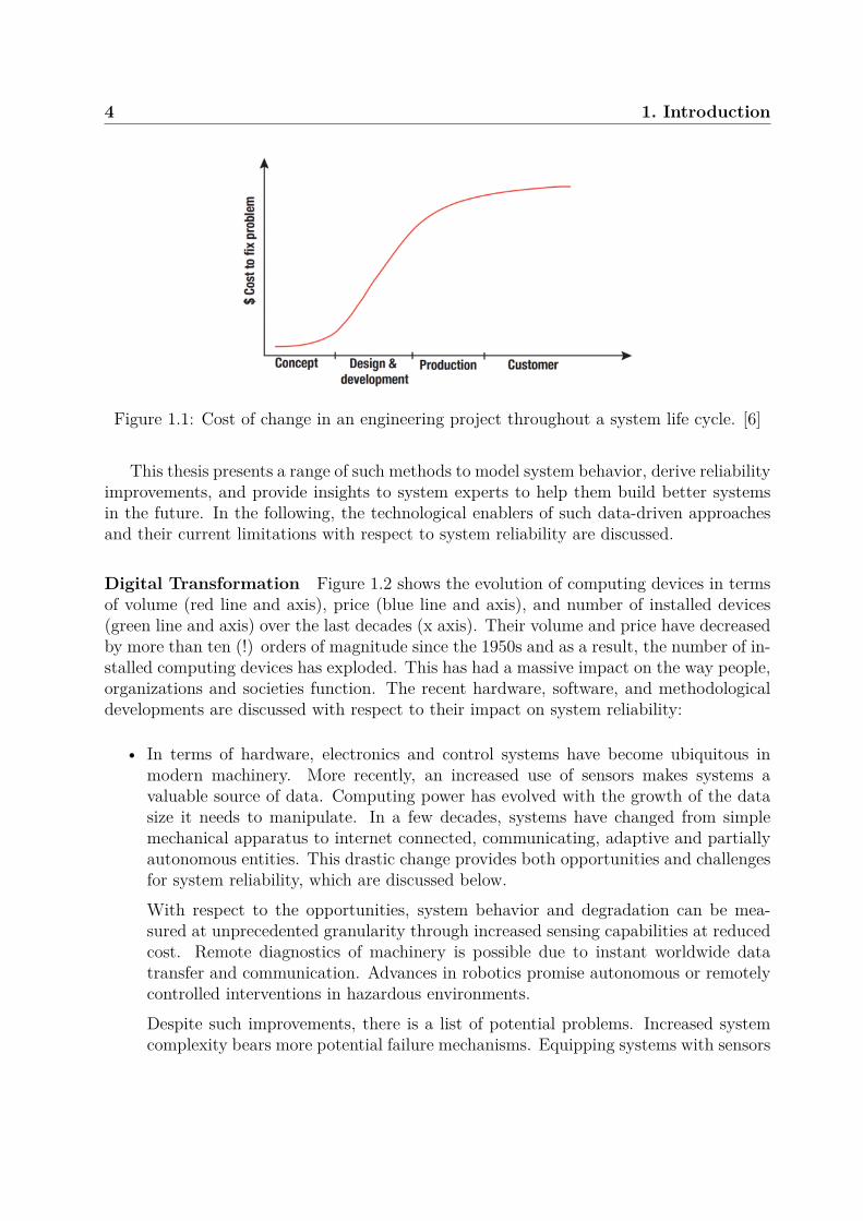
Figure 2.1: Schematic overview of the CERN accelerator complex. [29]
size and energy. Protons are accelerated by LINAC4, PS-BOOSTER (PSB), PS, andSPS before entering the LHC. Ions pass through LINAC3, LEIR, PS and SPS. This isillustrated in Figure 2.1. The solid lines in different colors depict the different particleaccelerators and the arrows the direction in which the particles move. The yellow dotsmark the four particle collision points of the LHC, as previously described. One can seethat a vast network of particle accelerators is operational at CERN. The oldest accelerator(the Proton Synchrotron - PS) dates back to 1959 and has been continuously maintainedand upgraded. For the operation of the LHC, all injectors need to be working at the sametime in a coordinated manner, which poses significant reliability challenges.
16 2. Particle Accelerators
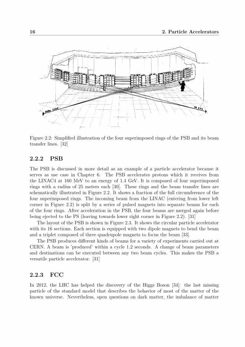
Figure 2.2: Simplified illustration of the four superimposed rings of the PSB and its beamtransfer lines. [32]
2.2.2 PSBThe PSB is discussed in more detail as an example of a particle accelerator because itserves as use case in Chapter 6. The PSB accelerates protons which it receives fromthe LINAC4 at 160 MeV to an energy of 1.4 GeV. It is composed of four superimposedrings with a radius of 25 meters each [30]. These rings and the beam transfer lines areschematically illustrated in Figure 2.2. It shows a fraction of the full circumference of thefour superimposed rings. The incoming beam from the LINAC (entering from lower leftcorner in Figure 2.2) is split by a series of pulsed magnets into separate beams for eachof the four rings. After acceleration in the PSB, the four beams are merged again beforebeing ejected to the PS (leaving towards lower right corner in Figure 2.2). [31]
The layout of the PSB is shown in Figure 2.3. It shows the circular particle acceleratorwith its 16 sections. Each section is equipped with two dipole magnets to bend the beamand a triplet composed of three quadrupole magnets to focus the beam [33].
The PSB produces different kinds of beams for a variety of experiments carried out atCERN. A beam is ’produced’ within a cycle 1.2 seconds. A change of beam parametersand destinations can be executed between any two beam cycles. This makes the PSB aversatile particle accelerator. [31]
2.2.3 FCCIn 2012, the LHC has helped the discovery of the Higgs Boson [34]: the last missingparticle of the standard model that describes the behavior of most of the matter of theknown universe. Nevertheless, open questions on dark matter, the imbalance of matter

2.3 Existing and Future Reliability Challenges for Particle Accelerators 17
Figure 2.3: Layout of the PSB and its beam transfer lines. [33]
and antimatter, and neutrino masses remain. Pushing the energy and precision frontierby building larger and more powerful accelerators is expected to shine light on these phe-nomena. Following the 2013 update of the European Strategy for Particle Physics [2], theFuture Circular Collider (FCC) study was launched at CERN to study options of protonand electron colliders at unprecedented energy levels as well as the required acceleratortechnology advancements.
Among the study’s main results is the proposition of a 100km tunnel to house anelectron collider (FCC-ee) which is later replaced by a hadron machine (FCC-hh) reachingcollision energies of 100 TeV. The recent 2020 update of the European Strategy for ParticlePhysics [3] supports further in-depth financial and technical feasibility studies for an FCC.
2.3 Existing and Future Reliability Challenges for Par-ticle Accelerators
To carry out scientific measurements effectively, it is important that particle acceleratorsdeliver the desired beam collisions whenever required. Thus, the particle accelerator andits many sub-systems must be reliable. Considering that particle accelerators often usemany complex sub-systems, which can be at technological frontiers and are produced insmall quantities, achieving high reliability can be challenging.

18 2. Particle Accelerators
Standard components of suppliers are often not qualified for use in particle acceleratorsas suppliers have optimized their products for use in the main markets, such as consumerelectronics with much shorter life time requirements. Another limitation is that systemsin particle accelerators are often exposed to radiation. Specialized equipment for suchenvironments is costly and standard systems require specialized qualification campaignsfor usage in radiation environments [35].
The life cycle of a particle accelerator can span several decades. Within such longperiods, technologies evolve and specific expertise needs to be passed along generationsof engineers. The sheer size of machines, such as the LHC, cause maintenance challengedue to the long distances to intervention sites. These factors pose further challenges inachieving high reliability.
However, there are also factors that facilitate reliability projects for particle accelerators.Many of their sub-systems are developed, built, operated, and maintained in-house. Thisrenders reliability efforts which aim at the whole system life cycle easier in comparison toindustries where systems are handed over to costumers after production and follow up onreliability is more difficult. Additionally, particle accelerator systems are often operated inenvironments with controlled temperature and humidity.
With the push to higher collision energies, future particle accelerators are expected toincrease in size, energy, and complexity by an order of magnitude in comparison to theLHC. This generally translates to much stricter reliability requirements for each of thesub-systems of a future particle accelerator to maintain LHC availability levels. At thesame time, the existing reliability challenges will be exacerbated by the increased size,complexity, levels of radiation, and further specialization of employed technologies.
If existing strategies to achieve reliable systems are maintained, the reliability goals offuture particle accelerators will not be met. Hence, new methods for reliability improve-ment have to be investigated.
In a range of potential strategies to overcome these challenges, data-driven methodspromise to improve the reliability of systems despite increases of complexity at moderateinvestment costs. This thesis develops quantitative reliability optimization methods toimprove the reliability of particle accelerator systems by deriving reliability improvementsfrom the operational history of existing systems. The main subject of study are magnetpower converters, which are introduced in the following. The developed methods can begeneralized to other kinds of systems.
2.4 Magnet Power ConvertersMagnet power converters supply a specific voltage and current waveform to magnets. Thecontrolled current in the magnets produce magnetic fields that precisely bend particlebeams through the Lorentz force. A schematic overview of a power converter is given inFigure 2.4. It consists of a power part, a measurement part and a control part.
The power part receives electric power from an electric supply network and provides thepower to the magnetic circuit. The input can be alternating or direct current. The output

2.4 Magnet Power Converters 19
Figure 2.4: Schematic overview of a power converter.
can take any desired waveform depending on the type of power converter. The poweris transformed in power electronics drive stages. The key types include power diodes,Bipolar Junction Transistor (BJT), Metal–Oxide–Semiconductor Field-Effect Transistors(MOSFET), Insulated-Gate Bipolar Transistors (IGBT), and thyristors. Heat dissipationfrom power electronics can require active air or water cooling systems.
The measurement part senses the actual voltage and current supplied to the magnetcircuit. The control part (Function Generation Controller in Figure 2.4) receives the desiredoutput waveform from a centralized control system and regulates the power part to obtainit at the output. It requires electronics hardware and software to translate the input signalsfrom the control system into the desired output waveform of the power converter.
External interlock signals for machine protection and safety purposes allow shuttingdown the power converter operation in a safe manner. Additional magnet protection sys-tems ensure that the energy stored in the magnetic circuit cannot cause damage. Thepower converter parts can be combined in dedicated racks. Configurations with line re-placeable units (LRU) allow to carry out repairs by replacing faulty units. Thereby, repairtimes are reduced.
The control part collects monitoring and diagnostics data for the power converter. Thefollowing data are commonly collected:
• Desired and actual voltage and current.
• Warnings, which indicate an error but do not lead to shut down of the converter.
• Faults, which indicate an error and lead to immediate shut down of the converter.
• Depending on the converter type additional monitoring signals, such as the temper-ature, radiation levels, or current to ground, are collected.
Such operational data is used for the data-driven reliability studies presented in this thesis.

20 2. Particle Accelerators
Chapter Learning Summary
The next generation of particle accelerators is expected to be more complex thanexisting infrastructures. Reliability approaches used for existing accelerators will notlead to a satisfying operational reliability of such future infrastructures.

Chapter 3
Backgrounds
3.1 Reliability Engineering
Reliability engineering is an engineering discipline for applying scientific know-how to asystem (component, product, plant, or process) in order to ensure that it performs itsintended function, without failure, for the required time duration in a specified environment[36]. A system S is defined as an aggregation of entities with a defined purpose. It hasa range of inputs I and outputs O through which it serves its intended purpose and it isseparated from its environment E through a boundary.
A system has a failure F when it fails to serve its purpose despite its environment andinputs being within specifications. The failure can be characterized by a range of properties,which are presented in Table 3.1. The first column shows the different terms to describea failure. The second column defines the terms of the first column. The second to fifthcolumns show four different failure examples with their corresponding failure description.
Generally, operating systems leads to loads, which depend on system input, output andenvironment. The loads cause internal stresses, which can lead to failures through specificmechanisms.
In the broken phone screen example in Table 3.1, a very high load leads to overstressand immediate failure. In this case, the load history of the screen is not relevant as thefailure would both occur in a new or old glass under the applied force. Contrary, in theworn car tyre example, the history of loads reduces the tyre profile through a so-calleddegradation or wear-out process. It is important to point out that the degradation-type offailure can be forecasted easier due to its gradual development in time.
The first two failure examples are hardware faults with mechanical loads and stresses.Hardware failures can also be driven by electrical, thermal, chemical, and other physicalstresses. The third and fourth example are software failures. The failure property con-cepts were developed for the physical nature of hardware faults. Hence, they apply lessintuitively to software failures, which are of discrete and non-physical nature. In the thirdexample, an overstress concept still applies as the server demand exceeds its capacity. Thisis comparable to the mechanical force exceeding the strength of the phone screen glass in

22 3. BackgroundsTa
ble3.1:
Failu
reconcepts
anddefin
ition
swith
hypo
thetical
exam
ples.
Ter
m
Def
init
ion
E
xa
mp
le 1
: E
xa
mp
le 2
: E
xa
mp
le 3
: E
xa
mp
le 4
:
Fail
ure
/Fa
ult
Sy
stem
fai
ls t
o s
erv
e
its
pu
rpose
des
pit
e it
s
env
iron
men
t an
d
inpu
ts b
ein
g w
ith
in
spec
ific
atio
ns
Bro
ken
ph
on
e sc
reen
W
orn
car
ty
res
Str
eam
ing
pla
tfo
rm
mal
fun
ctio
n
Sh
opp
ing
web
site
not
funct
ion
al
Fail
ure
mod
e T
he
ob
serv
able
eff
ect
of
a fa
ilu
re
Bro
ken
ph
on
e sc
reen
gla
ss a
fter
pho
ne
dro
pp
ed o
n t
ile
from
less
th
an h
alf
a m
eter
hei
gh
t.
Car
ty
res
wit
ho
ut
pro
file
afte
r d
rivin
g l
ess
than
1000
0k
m
Vid
eo s
trea
ms
kee
p
inte
rrup
ting
and
vid
eos
are
in l
ow
res
olu
tion
Sh
opp
ing
web
site
does
not
allo
w t
o p
ut
pro
du
cts
into
shop
pin
g c
art
Fail
ure
sit
e T
he
loca
tion
of
the
fail
ure
The
area
wher
e th
e
gla
ss i
s bro
ken
T
yre
pro
file
n
ot
appli
cab
le
not
appli
cab
le
Fail
ure
mec
ha
nis
m
The
pro
cess
th
at l
eads
to a
fai
lure
Mec
han
ical
over
stre
ss
Wea
rou
t du
e to
fri
ctio
n
Str
eam
ing
ser
ver
cap
acit
y d
oes
not
mee
t
dem
and
Hyp
erli
nk
are
a is
lo
cate
d
away
fro
m h
yp
erli
nk
tex
t
Fail
ure
str
ess
The
dri
vin
g f
orc
e of
the
fail
ure
mec
han
ism
M
echan
ical
str
ess
Mec
han
ical
str
ess
Num
ber
of
stre
amin
g
requ
ests
fro
m u
sers
Web
bro
wse
r an
d
oper
atin
g s
yst
em o
f use
r
Fail
ure
Lo
ad
The
appli
cati
on
or
env
iron
men
tal
con
dit
ion
wh
ich
cause
s st
ress
Fo
rce
acti
ng
on
scre
en
Con
tact
fo
rce
bet
wee
n
car
tyre
an
d r
oad
su
rfac
e
Num
ber
of
stre
amin
g
requ
ests
fro
m u
sers
Req
ues
t to
put
pro
duct
into
sh
opp
ing
car
t
Roo
t ca
use
(tec
hn
ical)
The
roo
t ca
use
is
the
most
bas
ic c
ausa
l
fact
or
or
fact
ors
th
at,
if c
orr
ecte
d o
r
rem
ov
ed,
Gla
ss m
oun
ted
und
er
too
hig
h s
tres
s
Wro
ng
mix
of
tyre
rubb
er
Co
mp
uti
ng
cap
acit
y i
s
too
sm
all
to m
eet
pee
k
dem
and
Fai
lure
occ
urs
bec
ause
of
unex
pec
ted
GU
I re
nder
ing
on
use
r's
oper
atin
g s
yst
em
and
web
bro
wse
r.
Roo
t ca
use
(org
an
iza
tio
nal)
The
roo
t ca
use
is
the
most
bas
ic c
ausa
l
fact
or
or
fact
ors
th
at,
if c
orr
ecte
d o
r
rem
ov
ed,
Und
er c
ost
pre
ssu
re,
an o
ld g
lass
mou
nti
ng
mac
hin
e
was
adop
ted
impro
per
ly f
or
pro
du
ctio
n o
f a
new
phon
e
The
gra
ph
ical
inte
rfac
e
of
the
tyre
rub
ber
mix
ing
mac
hin
e is
not
intu
itiv
e.
The
op
erat
or
was
not
able
to
ente
r th
e co
rrec
t
val
ues
und
er t
ime
pre
ssu
re.
Co
mp
uti
ng
cap
acit
y
was
dim
ensi
on
ed t
o
mee
t d
eman
d 9
9.9
% o
f
tim
es d
ue
to c
ost
pre
ssu
re a
nd
eff
icie
ncy
requ
irem
ents
.
Web
site
was
tes
ted
an
d
opti
miz
ed f
or
thre
e m
ost
popu
lar
bro
wse
rs a
nd
thre
e m
ost
pop
ula
r
oper
atin
g s
yst
ems.
Co
st
and
tim
e pre
ssu
re d
oes
no
t
allo
w e
xte
nsi
ve
test
ing
.

3.1 Reliability Engineering 23
the first example, albeit in a reversible manner. In the fourth example, the concept ofstress does not apply as the failure is due to a configurational incompatibility.
Quantitative Reliability Concepts The previous Section summarized the most im-portant qualitative features of failures. To quantify and communicate the reliability ofsystems, several mathematical concepts based on continuous probability functions havebeen introduced.1
The probability that a system S is functional at time t is given by its reliability functionR(t) ∈ [0, 1]. Likewise, the probability of having failed up to time t is given by thecumulative probability of failure (cdf),
F (t) = 1−R(t). (3.1)
For a fleet (also called population) of n identical systems, the cumulative probability offailure can be approximated by the ratio of failed systems, F (t) ≈ F (t) = nf (t)/n, withnf (t) being the number of failed systems at time t.
If a system or component has multiple failure mechanisms, they can be aggregated tocalculate the combined failure behavior. For independently competing failure mechanisms(i.e. one failure does not trigger another failure), the cumulative probability of failure(cdf) of a system with M different failure mechanisms, each described by separate cdfsFj(t), j = 1, ...,M , is given by [37]
¯F (t) =M∏j=1
Fj(t). (3.2)
The probability that a system fails within a time increment [t, t + dt] is given by itsfailure probability density (pdf) f(t)dt, which is the time derivative of the cumulativeprobability of failure,
F (t) =∫ t
−∞f(t)dt. (3.3)
The failure probability density can be approximated by generating a normalized histogramof the time-to-failure T of each system in a fleet.
The hazard rate h(t) describes the rate of failures per time per functional systems,
h(t) = f(t)R(t) . (3.4)
It allows to distinguish three different failure behaviors: A decreasing, constant or increas-ing hazard rate. Decreasing hazard rates may occur when manufacturing errors lead tofailures at the beginning of system use. This is called infant mortality. Systems with in-fant mortality can be screened before they are put into operation. This, so-called, burn-inremoves systems from the population that would fail early. Some system exhibit constant
1The explanations below follow the contents of standard reliability textbooks [8, 6].

24 3. Backgrounds
failure rates, especially due to failures of non-physical nature - e.g. improper use. Mostsystems will degrade and wear-out after some usage time, which leads to an increasinghazard rate.
The first moment of the failure probability density function (pdf),
E[T ] = µ =∫ +∞
−∞tf(t)dt, (3.5)
is the Mean Time To Failure (MTTF) [8]. Naturally, the expressiveness of the mean islimited for systems with non-constant failure behavior over time. It is possible to use highermoments of the pdf to describe the behavior more accurately, or resort to parametricon non-parametric models to quantify system reliability, which are covered later in thisSection.
The evolution of input, output and environment properties, as well as loads and stressesof systems over time can be expressed as (vector-)valued functions, I(t), O(t), E(t), L(t)and ξ(t), respectively.
Repairable Systems The introduced quantitative reliability concepts apply to non-repairable systems. For repairable systems, the methods have to be extended to modelconsecutive failures in time and the repair and maintenance activities.
The MTBF is the Mean Time Between Failures [8]. It can be calculated by averaging thetimes a system works between consecutive failures. It can include maintenance activities,which reduce the effective number of failures. Therefore, it shall not be confused with theMTTF. The average duration of repair is expressed as Mean Time To Repair (MTTR) [8].The system availability is given by,
A = time functional
time functional + time nonfunctional= uptime
uptime+ downtime. (3.6)
It asymptotically converges to
A∞ = MTBF/(MTBF +MTTR). (3.7)
Note that operational interruptions due to planned scheduled maintenance do not countas downtime. Downtime occurs when the system is not functional despite being expectedto function.
Quantitative Reliability Modeling Reliability modeling allows to predict the systembehavior as a function of any relevant factors during a system life cycle. Relevant factorsusually include the operating conditions, manufacturing techniques, design choices, andcomponent supplier selection of a system but may also consider less tangible factors suchas the logistics and storage history of systems, the experience of maintenance teams, etc.For the sake of brevity, all potentially relevant factors during a system life cycle can be

3.1 Reliability Engineering 25
denoted as X and the reliability metrics describing system behavior as Y. Then, theproblem of reliability modeling can be expressed as,
Y ≈ Φ(X), (3.8)with Φ(·) being the reliability model, often using a probabilistic formulation. The moreaccurate and the earlier in a system life cycle a the reliability model is available, thegreater its potential value for driving correct decisions and cost savings, according to Fig-ure 1.1. Finding accurate reliability models and using them for deriving general permanentreliability improvements within organizational contexts is the focus of this thesis. Thereare different strategies to obtain such models. A distinction is commonly made betweendata-driven, knowledge- (also model- or physics-) driven and hybrid approaches.
In a data-driven approach, the reliability model Φ(·) is automatically inferred fromobserved data (X and Y) using statistical and ML methods. This will be discussed indetail in a separate Section on ML techniques (see Section 3.3). For example, the profiledepth of a car tyre can be measured at different mileages. Then, X would be the recordedmileage, Y would be the corresponding profile depth, and the reliability model Y ≈ Φ(X)can be obtained by regression. The obtained model can predict profile wear based onmileage. However, the model implicitly assumes a certain type of tyre, car and usageprofile. I.e. it cannot be used to predict tyre wear for another kind of tyre, car or usagecondition. It is only valid under the conditions in which the training data was generated.This is one of the major limitations of data-driven methods.
In the knowledge-driven approach, the reliability model Φ(·) is built from first princi-ples, based on the a priori knowledge about the system and the problem domain. For thecar tyre example, a model of tyre wear can be derived with physical knowledge. It couldbe based on the mechanical properties of the rubber a, the weight (distribution) of the carb, the usage conditions c, and the strength of the car’s engine d. The model could take theform Y ≈ Φ(X; a, b, c, d). The set a, b, c, d = θ are called parameters of the model. Theycan be either be known from physics and domain knowledge or derived in experiments.Such a model can be used for different tyres, cars, and usage conditions as they are explic-itly modeled. Hence, in principle it can be considered superior to the data-driven modelof tyre wear. However, in many realistic settings, knowledge-driven models are either notavailable or inaccurate.
In practice, modeling methods contain both data and knowledge-driven componentsand can be considered hybrids. The parameter values and the model structure can beknown in advance or need to be determined from measurement data. Depending on theratio of data and knowledge-driven components in a model, they are classified respectively.The modeling approaches in Chapter 6 and 8 are mostly data-driven, whereas the methodin Chapter 7 is a hybrid method.
A particularly useful and popular function for modeling reliability problems is thetwo-parameter Weibull distribution [38]. It models the reliability of a system with twoparameters,
R(t) = exp−( t
η
)β . (3.9)

26 3. Backgrounds
Its first parameter, η, characterizes the lifetime t at which 63.2% of the population of sys-tems has failed. It is called characteristic lifetime or scale parameter. Its second parameter,β, allows to model an increasing, constant, or decreasing hazard rate when setting β > 1,β = 1, or β < 1, respectively.
Due to its simplicity, it can be useful to quickly identify whether a population ofsystems exhibits unusual hazard rates. However, it cannot model arbitrary fault timedistributions due to its limited set of parameters. Generally, it is advisable to visualize thefailure characteristics of data sets before assuming that they follow any specific parametricmodel.
Maintenance Strategies and Fault Tolerant Systems Maintenance is defined as anyactivity intended to retain or restore a system in or to a specified state in which the systemcan perform its required purpose [39]. This includes tests, measurements, replacements,adjustments, and repairs. It aims to maintain or increase the reliability of a system duringits operational lifetime.
The historically most common approach to maintenance is to run a system until it failsand return it to a functional state thereafter. This is called reactive maintenance. Sincesystems may have very high downtime costs, preventive maintenance techniques have beendeveloped to avoid failures. E.g., drive belts could be regularly replaced to avoid failures.Nevertheless, for certain systems in non-critical applications, reactive maintenance can bethe most cost-effective strategy. A trivial example is a living room light bulb for which aregular replacement before a failure occurs would only increase the operational cost andbear almost no practical advantage.
In the common time or cycle-based preventive maintenance method, maintenance iscarried out according to a fixed schedule. For example, the oil in a combustion engineis replaced after a fixed mileage and some airplane checks are performed after a certainamount of hours in flight. Such a maintenance strategy can increase the system lifetime andprevent unplanned breakdown. However, maintenance plans are often very conservativeand result in unnecessarily frequent interventions.
It is important to know the hazard rate of the system for which maintenance is carriedout. For systems with decreasing hazard rates, preventive maintenance can lead to morefrequent faults because the new replacing systems exhibit a higher failure rate than thereplaced ones. When hazard rates are constant, preventive replacements do not change thefrequency of faults, but increase the cost.
To address these limitations, condition-based maintenance has been introduced. Theidea is to measure or infer the health of a system and perform planned maintenance shortlybefore the system is about to fail. It promises to increase the reliability of systems incomparison to reactive maintenance by repairing or replacing systems before they fail. Incomparison to preventive maintenance, it promises to decrease the maintenance costs asunnecessary actions are not carried out.
Although superior in theory, the main drawback of this method is that it requires thecondition of a system to be measurable and failures predictable at a cost lower than the

3.1 Reliability Engineering 27
promised savings in comparison to reactive and preventive maintenance. This is the casefor systems such as car tyres, for which the profile depth can be easily measured at acost much lower than the tyre. However, for low cost electronic components, the cost ofmeasuring their condition may exceed their value by far.
Condition monitoring may still be justifiable if the failure of such low cost componentscauses a high financial loss. However, a better strategy might be to employ some form ofredundancy, which ensures a functional system despite failures of some of its components.This concept is called fault tolerance and it relies on four principles [40]: Redundancy,Fault Isolation, Fault Detection And Notification, and On-Line or Scheduled Repair. Re-dundancy means that the functionality of a system is distributed over several sub-systems.Then, the overall system can carry out its function despite failure of one or several sub-systems. Fault isolation requires that a failure in one sub-system cannot propagate to othersub-systems, causing a chain of failures. Protective devices, local separation, and variationof sub-systems can ensure this. Fault detection and notification implies that faults do notremain undetected when a sub-system fails and that a repair team gets notified. Finally,after the repair team gets informed, it has to carry out the repair of the failed sub-systemeither during operation or in a scheduled maintenance stop.
This approach allows to achieve close to 100% availability. Nevertheless, in practicesuch fault tolerant systems usually have design trade-offs which renders them vulnerable tocertain attacks or simultaneous failures of several sub-systems. However, the probability ofoccurrence of such events can be reduced to a minimum for real systems. E.g., flight controlcomputers (See e.g. [41, 42]) conform to these principles and achieve quasi-continuousavailability in operation. A closer look at the robustness of biological systems reveal similarprinciples at even higher levels of sophistication [43].
Cost models Cost models have been developed to quantify and compare the operationalcost of different maintenance and operational strategies. This thesis uses an adaptationof the models proposed by Vachtsevanos et al [44] for electronic and electrical hardwaresystems, which are the primary subject of investigations. It is composed of the cost of theequipment (design, development, material, and production costs) ceq, the cost of repairand maintenance activities Cr, and the cost due to downtime Cd. Adding these costs, theoverall life cycle cost can be expressed as,
C = Ceq + Cr + Cd, (3.10)
in a general form. Assuming an average cost per repair of internal failures cr and an averagecost per unplanned downtime event cd, the cost can be expressed as
C = neqceq + nrcr + ndcd, (3.11)
with nr being the number of repairs, nd being the number of downtime events during thesystem lifetime, and neq the equipment cost factor to consider redundant configurations oradditional costs for condition monitoring. The formula can be generalized to account fordifferent failure modes and corresponding repair actions.

28 3. Backgrounds
The expression can be exemplified by comparing the cost of reactive, preventive, condition-based maintenance, and fault tolerance solutions for a hypothetical power converter ex-ample. In corrective maintenance, a system is run until it fails. Hence, the number ofdowntime occurrences equals the number of repairs, nr,corr = nd,corr. For preventive main-tenance, the system will be repaired before it fails. However, sometimes the system may failduring operation, 0 ≤ nd,prev ≤ nd,corr. Still, the number of repairs will be larger than thenumber of downtime occurrences, nr,prev > nd,prev. For condition-based maintenance, thesituation is similar to preventive maintenance. However, due to condition inspection, thetiming of maintenance is expected to be more precise. Hence, less downtime occurrencesand less repairs can be expected. The condition monitoring requires additional equipmentinvestment for sensors or routine inspections (here the inspection costs are seen as part ofequipment costs). For fault tolerance, downtime occurrences can practically be eliminated.Load sharing on several redundant systems can lead to longer lifetimes due to lower stresslevels. However, the required redundancy leads to additional equipment cost.
Figures 3.1a and 3.1b show the life cycle cost for different maintenance strategies for twohypothetical power converters with low (ceq,a = 100) and high (ceq,b = 10000) equipmentcost, respectively. The y axis shows the life cycle cost for the four different operationalstrategies; corrective, preventive, condition-based maintenance, and fault-tolerance, de-noted on the x axis. The color code marks the cost contribution due to equipment costs(blue), repair cost (orange), and downtime cost (grey). In both cases the cost of repair cris 100, the cost of a downtime occurrence cd is 1000, and the cost of condition monitoringis 100. However, depending on the equipment cost, the relative cost of the different oper-ational strategies varies greatly. Hence, choosing the correct operational strategy dependson various cost factors as well as the failure behavior of the considered system.
Table 3.2 lists the assumed numbers of repairs, downtime occurrences, and the equip-ment cost (including condition monitoring and redundancy) in each row for the four dif-ferent operational strategies in each column. The equipment cost is the only factor thatchanges between the two scenarios. For low equipment costs, redundancy is the mostcost-effective solution. For high equipment costs, condition-based maintenance is morecost-effective in this hypothetical example. Similar relations are observed in realistic set-tings [24, 45] and in the investigated scenario in Chapter 7.
Reliability Simulation The operation of a system can be simulated to evaluate differentoperational and maintenance strategies and their associated costs. This requires a relia-bility model (equation 3.8), an operational cost model (equation 3.11), and a simulationengine. Due to the probabilistic nature of failures and the statistical concepts describingthem, Monte Carlo simulations [46, 47] are often employed as simulation methods. Theprinciple is to carry out multiple simulations with parameters drawn from their probabilitydistribution. The results of all simulations are collected and their statistics calculated.
Thereby, different parameters and scenarios can be studied over the expected life cycleof a system. Based on the results, the set of parameters with the best outcome in termsof life cycle cost or reliability can be recommended to decision makers. Further details of

3.1 Reliability Engineering 29
0
2000
4000
6000
8000
10000
12000
Corrective Preventive Condition-Based Fault-Tolerant
Co
st
Equipment Cost Repair Cost Downtime Cost
(a)
0
5000
10000
15000
20000
25000
Corrective Preventive Condition-Based Fault-Tolerant
Co
st
Equipment Cost Repair Cost Downtime Cost
(b)
Figure 3.1: Life cycle cost for different maintenance strategies for a hypothetical examplewith (a) low equipment cost and (b) high equipment cost. For low equipment cost, faulttolerance is the most cost-effective solution. For high equipment cost, condition-basedmaintenance is the most cost-effective solution.
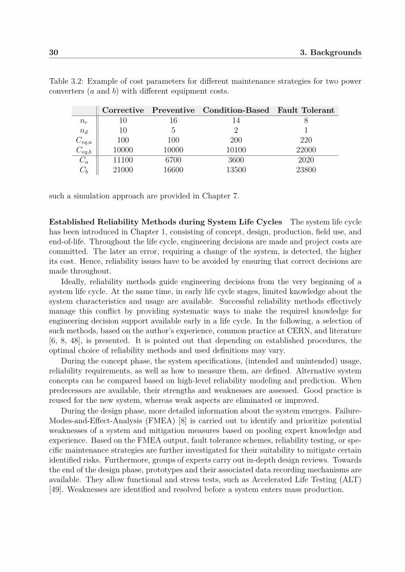
30 3. Backgrounds
Table 3.2: Example of cost parameters for different maintenance strategies for two powerconverters (a and b) with different equipment costs.
Corrective Preventive Condition-Based Fault Tolerantnr 10 16 14 8nd 10 5 2 1Ceq,a 100 100 200 220Ceq,b 10000 10000 10100 22000Ca 11100 6700 3600 2020Cb 21000 16600 13500 23800
such a simulation approach are provided in Chapter 7.
Established Reliability Methods during System Life Cycles The system life cyclehas been introduced in Chapter 1, consisting of concept, design, production, field use, andend-of-life. Throughout the life cycle, engineering decisions are made and project costs arecommitted. The later an error, requiring a change of the system, is detected, the higherits cost. Hence, reliability issues have to be avoided by ensuring that correct decisions aremade throughout.
Ideally, reliability methods guide engineering decisions from the very beginning of asystem life cycle. At the same time, in early life cycle stages, limited knowledge about thesystem characteristics and usage are available. Successful reliability methods effectivelymanage this conflict by providing systematic ways to make the required knowledge forengineering decision support available early in a life cycle. In the following, a selection ofsuch methods, based on the author’s experience, common practice at CERN, and literature[6, 8, 48], is presented. It is pointed out that depending on established procedures, theoptimal choice of reliability methods and used definitions may vary.
During the concept phase, the system specifications, (intended and unintended) usage,reliability requirements, as well as how to measure them, are defined. Alternative systemconcepts can be compared based on high-level reliability modeling and prediction. Whenpredecessors are available, their strengths and weaknesses are assessed. Good practice isreused for the new system, whereas weak aspects are eliminated or improved.
During the design phase, more detailed information about the system emerges. Failure-Modes-and-Effect-Analysis (FMEA) [8] is carried out to identify and prioritize potentialweaknesses of a system and mitigation measures based on pooling expert knowledge andexperience. Based on the FMEA output, fault tolerance schemes, reliability testing, or spe-cific maintenance strategies are further investigated for their suitability to mitigate certainidentified risks. Furthermore, groups of experts carry out in-depth design reviews. Towardsthe end of the design phase, prototypes and their associated data recording mechanisms areavailable. They allow functional and stress tests, such as Accelerated Life Testing (ALT)[49]. Weaknesses are identified and resolved before a system enters mass production.

3.2 Data, Information and Knowledge 31
During the production phase, various quality methods ensure conformance to produc-tion specifications. Functional (reception) tests can assure correct handling during allphases of production and assembly.
During field use, operation is monitored and failures are reported. Operational faultsneed to be analyzed by project stakeholders and mitigation measures identified. Repairand maintenance is carried out in either a reactive, preventive or condition-based manner.Depending on the behavior of the system, maintenance and operation strategies can beadapted.
During end-of-life, reusable parts of the system are identified. Strengths and weaknessesof the system are analyzed and communicated to future systems’ project teams with thegoal of achieving a continuous improvement of reliability and preventing repeated mistakes.As usually a range of comparable systems are managed at different life cycle stages at thesame time, insights obtained from one system can be utilized in other systems. Hence,communication of reliability insights to other project teams is advisable at all life cyclestages.
3.2 Data, Information and KnowledgeThe terms data, information and knowledge are used extensively throughout this thesis.To avoid confusion, the definition by Liew [50] is followed:
• "Data are recorded (captured and stored) symbols and signal readings. Symbols in-clude words (text and/or verbal), numbers, diagrams, and images (still &/or video),which are the building blocks of communication. Signals include sensor and/or sen-sory readings of light, sound, smell, taste, and touch. As symbols, ‘Data’ is thestorage of intrinsic meaning, a mere representation. The main purpose of data is torecord activities or situations, to attempt to capture the true picture or real event.Therefore, all data are historical, unless used for illustration purposes, such as fore-casting.
• Information is a message that contains relevant meaning, implication, or input fordecision and/or action. Information comes from both current (communication) andhistorical (processed data or ‘reconstructed picture’) sources. In essence, the purposeof information is to aid in making decisions and/or solving problems or realizing anopportunity.
• Knowledge is the (1) cognition or recognition (know-what), (2) capacity to act (know-how), and (3) understanding (know-why) that resides or is contained within the mindor in the brain. The purpose of knowledge is to better our lives. In the context ofbusiness, the purpose of knowledge is to create or increase value for the enterpriseand all its stakeholders. In short, the ultimate purpose of knowledge is for valuecreation."

32 3. Backgrounds
Liew explains further that the source of data and information lies in activities and situa-tions. In the case of reliability studies, activities could be repairing a system and situationscould be the condition leading to a fault of a system. These activities can be captured andstored in some database, which leads to data, and/or a human being can absorb and un-derstand the activities and situations, recognize relationships and derive desirable actions,which leads to knowledge.
In this thesis, methods are developed to effectively combine specialized data (of engi-neered systems as recorded in databases) with specialized knowledge (as internalized bysystem experts) to extract information and new knowledge to improve the reliability ofsystems cost-effectively.
3.3 Artificial Intelligence and Machine LearningIn a previous paragraph on reliability modeling, the data-driven approach was introduced.It is based on inferring the relationship between relevant factors during a system life cycleX and reliability metrics Y from observed data using ML. ML is a sub field of AI. AIis any kind of intelligence demonstrated by machines. ML is the ability of algorithms toimprove from experience, commonly encoded in data.
Supervised Machine Learning When the data is available in two sets, e.g. systemmonitoring data X and reliability metrics Y, and the goal is to learn a relation Y ≈Y = Φ(X) between the input data X and the target or output data Y, the task is calledsupervised learning. When the target data is discrete, the problem is called classificationand when the target data is continuous, the problem is referred to as regression. Thefollowing paragraphs give a practical introduction to the most relevant aspects of applyingML. Readers are forwarded to the literature for a more detailed treatment. E.g. the booksby Hastie et al [51] and Geron et al [52] are a good starting point and form the basis forthe following paragraphs.
Regression Contrary to the knowledge-driven approach, where a model Y ≈ Y = Φ(X)is derived from first principles, in the data-driven approach, it is learned from a train-ing data set Ytrain,Xtrain = (y1, ..., yN)train, (x1, ..., xN)train, with N being the number ofsamples in the data set.
This is exemplified on a hypothetical data set of car tyre profile wear. Figure 3.2shows the training data set. The blue dots depict the measured profile depth (y axis) as afunction of the mileage (x axis). The only feature of the data set is the mileage measured inkilometers and its target variable is the measured profile depth, which should be modeled.In the language of statistics, the mileage would be the independent variable and the profiledepth the dependent one.
The data was obtained by performing profile depth measurements for several cars onan irregular basis. It is known that the data is collected for a single type of tyre. Onlythe front right wheel was measured. The car types are not known. There are only a few

3.3 Artificial Intelligence and Machine Learning 33
10000 20000 30000 40000 50000Mileage [km]
0
2
4
Prof
ile [m
m]
Figure 3.2: Raw collected data of tyre wear.
0 10000 20000 30000 40000 50000Mileage [km]
0
2
4
Prof
ile [m
m]
Figure 3.3: Linear fit to raw data.
data points, which is common for reliability problems. Although many ML techniqueshave been developed for applications with large data sets, several methods perform wellon small data sets as well. In the following, a simple example of such a ML technique isintroduced and the common steps in a ML project are carried out.
One of the simplest models to express the observed relation is a linear model, Y =θ0 · X0 + θ1 · X1 = XT · θ. Its parameters θ = (θ0, θ1) are obtained by minimizing thesquared error, SE(θ) = ∑N
i=1(yi−xTi ·θ)2 = ∑Ni=1(yi− yi)2. The solid blue line in Figure 3.3
shows the best fit to the data obtained by the described linear regression principle.
Data Cleaning and Validation Notably, the function misses the evolution of the data.This is due to the many profile depth values that are zero. Apparently, some tyres arestill used despite not having any profile left. However, this is not the process that shouldbe modeled. Therefore, the data points with a profile depth of zero are removed from thedata set.
Such preliminary visualizations and tests are referred to as data cleaning and validation.It is one of the first and most important steps in a machine learning project as ML modelscan only be as accurate and valid as the data that describes the process of interest.
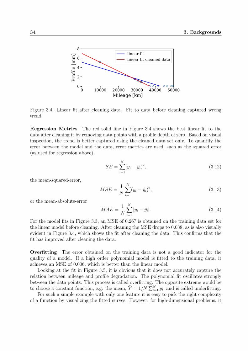
34 3. Backgrounds
0 10000 20000 30000 40000 50000Mileage [km]
0
2
4
6
8
Prof
ile [m
m] linear fit
linear fit cleaned data
Figure 3.4: Linear fit after cleaning data. Fit to data before cleaning captured wrongtrend.
Regression Metrics The red solid line in Figure 3.4 shows the best linear fit to thedata after cleaning it by removing data points with a profile depth of zero. Based on visualinspection, the trend is better captured using the cleaned data set only. To quantify theerror between the model and the data, error metrics are used, such as the squared error(as used for regression above),
SE =N∑i=1
(yi − yi)2, (3.12)
the mean-squared-error,
MSE = 1N
N∑i=1
(yi − yi)2, (3.13)
or the mean-absolute-errorMAE = 1
N
N∑i=1|yi − yi|. (3.14)
For the model fits in Figure 3.3, an MSE of 0.267 is obtained on the training data set forthe linear model before cleaning. After cleaning the MSE drops to 0.038, as is also visuallyevident in Figure 3.4, which shows the fit after cleaning the data. This confirms that thefit has improved after cleaning the data.
Overfitting The error obtained on the training data is not a good indicator for thequality of a model. If a high order polynomial model is fitted to the training data, itachieves an MSE of 0.006, which is better than the linear model.
Looking at the fit in Figure 3.5, it is obvious that it does not accurately capture therelation between mileage and profile degradation. The polynomial fit oscillates stronglybetween the data points. This process is called overfitting. The opposite extreme would beto choose a constant function, e.g. the mean, Y = 1/N ∑N
i=1 yi, and is called underfitting.For such a simple example with only one feature it is easy to pick the right complexity
of a function by visualizing the fitted curves. However, for high-dimensional problems, it
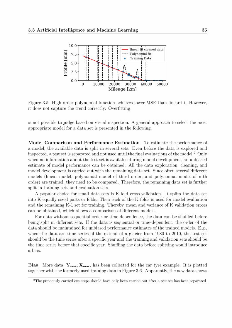
3.3 Artificial Intelligence and Machine Learning 35
0 10000 20000 30000 40000 50000Mileage [km]
0.0
2.5
5.0
7.5
10.0
Prof
ile [m
m] linear fit cleaned data
Polynomial fitTraining Data
Figure 3.5: High order polynomial function achieves lower MSE than linear fit. However,it does not capture the trend correctly: Overfitting
is not possible to judge based on visual inspection. A general approach to select the mostappropriate model for a data set is presented in the following.
Model Comparison and Performance Estimation To estimate the performance ofa model, the available data is split in several sets. Even before the data is explored andinspected, a test set is separated and not used until the final evaluations of the model.2 Onlywhen no information about the test set is available during model development, an unbiasedestimate of model performance can be obtained. All the data exploration, cleaning, andmodel development is carried out with the remaining data set. Since often several differentmodels (linear model, polynomial model of third order, and polynomial model of n-thorder) are trained, they need to be compared. Therefore, the remaining data set is furthersplit in training sets and evaluation sets.
A popular choice for small data sets is K-fold cross-validation. It splits the data setinto K equally sized parts or folds. Then each of the K folds is used for model evaluationand the remaining K-1 set for training. Thereby, mean and variance of K validation errorscan be obtained, which allows a comparison of different models.
For data without sequential order or time dependence, the data can be shuffled beforebeing split in different sets. If the data is sequential or time-dependent, the order of thedata should be maintained for unbiased performance estimates of the trained models. E.g.,when the data are time series of the extend of a glacier from 1980 to 2010, the test setshould be the time series after a specific year and the training and validation sets should bethe time series before that specific year. Shuffling the data before splitting would introducea bias.
Bias More data, Ynew,Xnew, has been collected for the car tyre example. It is plottedtogether with the formerly used training data in Figure 3.6. Apparently, the new data shows
2The previously carried out steps should have only been carried out after a test set has been separated.
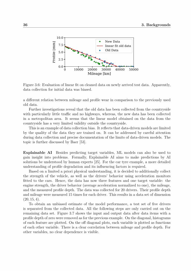
36 3. Backgrounds
0 10000 20000 30000 40000 50000Mileage [km]
0.0
2.5
5.0
7.5
10.0
Prof
ile [m
m] New Data
linear fit old dataOld Data
Figure 3.6: Evaluation of linear fit on cleaned data on newly arrived test data. Apparently,data collection for initial data was biased.
a different relation between mileage and profile wear in comparison to the previously usedold data.
Further investigations reveal that the old data has been collected from the countrysidewith particularly little traffic and no highways, whereas, the new data has been collectedin a metropolitan area. It seems that the linear model obtained on the data from thecountryside has a very limited validity outside the countryside.
This is an example of data collection bias. It reflects that data-driven models are limitedby the quality of the data they are trained on. It can be addressed by careful attentionduring data collection and precise documentation of the limits of data-driven models. Thetopic is further discussed by Baer [53].
Explainable AI Besides predicting target variables, ML models can also be used togain insight into problems. Formally, Explainable AI aims to make predictions by AIsolutions be understood by human experts [25]. For the car tyre example, a more detailedunderstanding of profile degradation and its influencing factors is required.
Based on a limited a priori physical understanding, it is decided to additionally collectthe strength of the vehicle, as well as the drivers’ behavior using acceleration monitorsfitted to the cars. Hence, the data has now three features and one target variable: theengine strength, the driver behavior (average acceleration normalized to one), the mileage,and the measured profile depth. The data was collected for 20 drivers. Their profile depthand mileage were measured 15 times for each driver. This results in a data set of dimension(20, 15, 4).
To obtain an unbiased estimate of the model performance, a test set of five driversis separated from the collected data. All the following steps are only carried out on theremaining data set. Figure 3.7 shows the input and output data after data items with aprofile depth of zero were removed as for the previous example. On the diagonal, histogramsof each feature are plotted. On the off diagonal plots, each variable is plotted as functionsof each other variable. There is a clear correlation between mileage and profile depth. Forother variables, no clear dependence is visible.

3.3 Artificial Intelligence and Machine Learning 37
50
100
Eng
ine
0.75
1.00
1.25
Beh
avio
ur
0
20000
Mile
age
50 100
Engine
0.0
2.5
5.0
Prof
ile
0.75
1.00
1.25
Behaviour
0
2000
0
Mileage
0 5
Profile
Figure 3.7: Scatter plot of new extended multivariate data set, containing engine strength,driver behavior, driven mileage, and tyre profile depth as variables. Histograms of eachvariable the diagonal. Scatter plots of all combinations of any two variables on off-diagonals.Clear dependence only visible for profile depth as function of mileage driven.
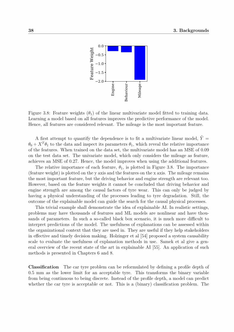
38 3. Backgrounds
Eng
ine
Beh
avio
ur
Mile
age
2.0
1.5
1.0
0.5
0.0
Feat
ure
Wei
ght
Figure 3.8: Feature weights (θ1) of the linear multivariate model fitted to training data.Learning a model based on all features improves the predictive performance of the model.Hence, all features are considered relevant. The mileage is the most important feature.
A first attempt to quantify the dependence is to fit a multivariate linear model, Y =θ0 +XT θ1 to the data and inspect its parameters θ1, which reveal the relative importanceof the features. When trained on the data set, the multivariate model has an MSE of 0.09on the test data set. The univariate model, which only considers the mileage as feature,achieves an MSE of 0.27. Hence, the model improves when using the additional features.
The relative importance of each feature, θ1, is plotted in Figure 3.8. The importance(feature weight) is plotted on the y axis and the features on the x axis. The mileage remainsthe most important feature, but the driving behavior and engine strength are relevant too.However, based on the feature weights it cannot be concluded that driving behavior andengine strength are among the causal factors of tyre wear. This can only be judged byhaving a physical understanding of the processes leading to tyre degradation. Still, theoutcome of the explainable model can guide the search for the causal physical processes.
This trivial example shall demonstrate the idea of explainable AI. In realistic settings,problems may have thousands of features and ML models are nonlinear and have thou-sands of parameters. In such a so-called black box scenario, it is much more difficult tointerpret predictions of the model. The usefulness of explanations can be assessed withinthe organizational context that they are used in. They are useful if they help stakeholdersin effective and timely decision making. Holzinger et al [54] proposed a system causabilityscale to evaluate the usefulness of explanation methods in use. Samek et al give a gen-eral overview of the recent state of the art in explainable AI [55]. An application of suchmethods is presented in Chapters 6 and 8.
Classification The car tyre problem can be reformulated by defining a profile depth of0.5 mm as the lower limit for an acceptable tyre. This transforms the binary variablefrom being continuous to being discrete. Instead of the profile depth, a model can predictwhether the car tyre is acceptable or not. This is a (binary) classification problem. The
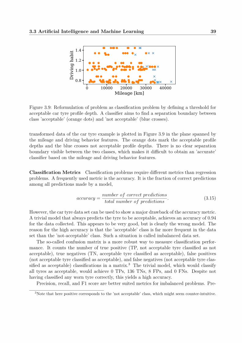
3.3 Artificial Intelligence and Machine Learning 39
0 10000 20000 30000 40000Mileage [km]
0.8
1.0
1.2
1.4
Dri
ving
hab
it
Figure 3.9: Reformulation of problem as classification problem by defining a threshold foracceptable car tyre profile depth. A classifier aims to find a separation boundary betweenclass ’acceptable’ (orange dots) and ’not acceptable’ (blue crosses).
transformed data of the car tyre example is plotted in Figure 3.9 in the plane spanned bythe mileage and driving behavior features. The orange dots mark the acceptable profiledepths and the blue crosses not acceptable profile depths. There is no clear separationboundary visible between the two classes, which makes it difficult to obtain an ’accurate’classifier based on the mileage and driving behavior features.
Classification Metrics Classification problems require different metrics than regressionproblems. A frequently used metric is the accuracy. It is the fraction of correct predictionsamong all predictions made by a model,
accuracy = number of correct predictions
total number of predictions. (3.15)
However, the car tyre data set can be used to show a major drawback of the accuracy metric.A trivial model that always predicts the tyre to be acceptable, achieves an accuracy of 0.94for the data collected. This appears to be very good, but is clearly the wrong model. Thereason for the high accuracy is that the ’acceptable’ class is far more frequent in the dataset than the ’not-acceptable’ class. Such a situation is called imbalanced data set.
The so-called confusion matrix is a more robust way to measure classification perfor-mance. It counts the number of true positive (TP, not acceptable tyre classified as notacceptable), true negatives (TN, acceptable tyre classified as acceptable), false positives(not acceptable tyre classified as acceptable), and false negatives (not acceptable tyre clas-sified as acceptable) classifications in a matrix.3 The trivial model, which would classifyall tyres as acceptable, would achieve 0 TPs, 136 TNs, 8 FPs, and 0 FNs. Despite nothaving classified any worn tyre correctly, this yields a high accuracy.
Precision, recall, and F1 score are better suited metrics for imbalanced problems. Pre-
3Note that here positive corresponds to the ’not acceptable’ class, which might seem counter-intuitive.

40 3. Backgrounds
cision is defined as the ratio of TPs over all positively classified items,
precision = TP
TP + FP. (3.16)
Recall is the fraction of TPs selected from all actually positive items,
recall = TP
TP + FN. (3.17)
The harmonic mean of precision and recall is the F1 score,
F1 = 2 · precision · recallprecision+ recall
. (3.18)
The trivial classifier would achieve a precision, recall and F1 of 0.
Imbalanced Learning In reliability problems, it is common to have imbalanced datasets, e.g. less examples of failed than functioning systems. It is often more important not toclassify an erroneous system as functioning (FN) than vice versa (FP). In such cases, classweights can be assigned to reflect that importance. Alternatively, so-called re-samplingstrategies can be employed. Thereby, either the more frequent class can be reduced (down-sampled) or the less frequent class can be expanded (up-sampled) until the desired classbalance is obtained. In the simplest case, random removal or duplication of data items isemployed. More complex sampling strategies, such as SMOTE [56], synthetically gener-ate data items which are similar to existing data items by using certain generation rules.For data accessible to human intuition, such as images or sound, it can easily be judgedwhether such rules are appropriate. E.g., for an image of a dog, a slight rotation or stretch-ing of the dog does not turn it into a cat. However, for more complex data, such as systemmonitoring data, it cannot be judged upfront whether certain transformations of the datachange its information content. Therefore, advanced sampling strategies need to be em-ployed with caution in complex data scenarios. An overview of strategies for imbalanceddata sets is provided by He et al [57] and an example of a sampling strategy for complexsystem monitoring data is provided in Chapter 6.
Learning Summary
Reliability Engineering is the technical discipline which aims to improve the relia-bility of systems. Recent developments in data science have the potential to lead tomethods for the cost-effective reliability optimization of systems.

Chapter 4
Literature Review
To gain an understanding of the state-of-the-art in the domain of data-driven reliabil-ity optimization, a literature review is carried out. This chapter addresses the relevantliterature shared by all research questions introduced in Chapter 1. Literature uniquelyrelated to each of the three scenario-specific research questions are presented separately inChapters 6-8, respectively.
An overview of the relevant research areas is given in Section 4.1. This includes thearea of analytics, reliability optimization, and prognostics. The section concludes witha definition of data-driven reliability optimization and discusses its relation to the otherrelevant research areas mentioned.
In Section 4.2, current limitations of data-driven reliability optimization are discussedwith a focus on the development, implementation, and adoption of such methods in orga-nizational contexts.
4.1 Literature OverviewData-driven reliability optimization as technical term is not frequently used in the reliabil-ity studies literature. Therefore, this section provides an overview of related research areasas well as a definition and demarcation of data-driven reliability optimization to other rele-vant research areas, such as prognostics in reliability engineering and the multidisciplinaryanalytics field.
Analytics Nelson [58] defines analytics as ’a comprehensive, data-driven strategy forproblem solving’. Its precise definition is under debate [59]. Generally, it can be viewed asthe connecting tissue between data and decision making and is a sub-field of the vaguelydefined data sciences.
The topic is divided in descriptive, predictive and prescriptive analytics, which aimto describe, predict or provide ways to change the outcome of a process, respectively.Analytics builds upon use of mathematics, statistics, data, and expert knowledge to createany form of benefit.

42 4. Literature Review
Reliability Optimization Reliability optimization aims to optimize an objective func-tion given decision variables and constraints. The objective function usually representsreliability or cost. The decision variables can be tuned to maximize the objective function.Examples include system configuration, component choice, and redundancy allocation. Theconstraints represent boundary conditions, such as physical, cost, or reliability constraints.[60]
Reliability optimization has been established in the mid of the twentieth century. Ithas evolved from static and exact to dynamic and approximate solutions for optimizationproblems to better reflect practical needs. Future challenges involve the integration of con-tinuous streams of data in modern interconnected systems, the ability to adapt to changingsystems and environments, and the accounting for uncertainties in the optimization pro-cess. [60, 61]
Prognostics Prognostics in engineering sciences is defined in ISO13381-1 as ’an estima-tion of time to failure and risk for one or more existing and future failure modes’ [62]. Assuch, it allows to perform predictive maintenance which leads to reduced operational costsof systems.
Defining Data-Driven Reliability Optimization Data-driven reliability optimiza-tion is the application of predictive and prescriptive analytics to reliability studies. Itsgoal is to increase the reliability of systems and decrease their life cycle costs. It sharesthe goals of reliability optimization and tackles its aforementioned open challenges withmodern analytics approaches.
(Data-driven) Prognostics can be classified as data-driven reliability optimization witha narrower objective of forecasting the precise end of life of certain systems and providestrategies to deal with it. As explained in Chapter 1, the biggest potential for reliabilityimprovement and life cycle cost savings is at the beginning of a system life cycle. However,prognostics acts at the end of the life cycle, which limits its potential benefits.
Data-driven reliability optimization aims to enable problem solving and decision makingat all stages of the system life cycle, particularly at early stages when the potential benefitsare largest.
Quantitative data-driven reliability optimization uses quantitative methods to achievethese goals. It is the primary topic of this thesis.
4.2 Existing Limitations of Data-Driven Frameworksfor Reliability Optimization
In this section, current limitations of data-driven reliability optimization are discussedwith a focus on the development, implementation, and adoption of such methods in or-ganizational contexts. A large fraction of available literature on data-driven reliabilityoptimization is focused on the sub-fields of prognostics and predictive maintenance. Since

4.2 Existing Limitations of Data-Driven Frameworks for ReliabilityOptimization 43
the general approach of prognostics overlaps with that of data-driven reliability studies,except for having narrower objectives, it is possible to generalize limitations from prog-nostics and predictive maintenance literature. Hence, the limitations outlined below arebased on a meta-review of survey and review articles in the fields of prognostics and gen-eral reliability engineering. These limitations are the inability of current methods to dealwith the complexity and uncertainty of realistic settings, that infrastructures cannot meetthe minimal requirements current methods pose, that organizations can not meet minimalrequirements of current methods, and that the focus of current methods on predictingremaining useful life is too narrow.
Complexity and Uncertainty in Realistic Reliability Problems Zio [63] statessystem modeling and representation, model quantification, and uncertainty-quantificationof model and system behavior as the main challenges of reliability engineering. Increasingfunctional requirements of modern systems often lead to systems at the frontier of tech-nology and complexity. Failures can always occur as emergent behavior when multiplesuch complex systems interact in dynamic environments. Good model representations andquantification for such failure behavior are almost impossible to provide. Reliability op-timization techniques have to continually evolve to match the complexity requirements ofmodern interconnected systems [60].
Data-driven reliability optimization methods struggle to keep up with the pace of tech-nological developments. Existing studies are mostly carried out on a component level, oftenconsidering only single failure modes. However, in reality systems are composed of manycomponents and are affected by multiple, often overlapping failure modes and mechanisms[17, 64, 65]. Many studies do not account for the dependence of failure mechanisms on mul-tiple factors [66]. Dynamic environments and unforeseen inputs can often not be robustlyhandled by data-driven methods [19]. Degradation does not only happen during operationof systems. Systems are exposed to stresses during transport, storage and installation,which can remain unobserved by monitoring systems.
The lack of suitability of developed methods for realistic problem settings is exemplifiedin an informal study by Hodkiewicz et al [16]. Of all 64 published papers in IEEE Trans-actions on Reliability in 2013 which proposed reliability models, they found that only in 7papers it was attempted to validate the developed methodologies with field data includingany description of the data collection.
Uncertainty in reliability problems arises from several sources. The limited knowledgeof the future usage of systems poses an irreducible uncertainty. Reducible uncertaintiesarise due to the limited available data of system degradation which is expensive to gen-erate, the limited understanding of failure mechanisms, and the limited availability ofaccurate modeling options [64]. Therefore, an uncertainty-quantification and propagationthroughout all steps in reliability modeling is essential. Some methods are suited for han-dling of uncertainty whereas others, such as neural networks, are less suited [67, 17]. Thelimitations of existing data-driven methods make industrial success stories rare [19, 17].

44 4. Literature Review
Infrastructures cannot Meet Minimal Requirements of Methods Proposed inLiterature Methods proposed in the literature frequently require a well-functioning mon-itoring of equipment and existing data sets of run to failure data. However, many organi-zations cannot meet these requirements [17]. Especially the required sensors and associ-ated data acquisition systems for monitoring are expensive to install in existing and newmachinery. Moreover, dedicated sensing equipment may be unreliable itself, can requiremaintenance, and needs regular calibration. Given that the expected benefits of such in-vestments are not certain, many organizations do not install dedicated sensor systems forreliability purposes [20, 21].
However, most machinery already log operational data through their control systems.This data may provide condition monitoring and reliability information at no additionalcost. Some successes using such data have already been reported [23].
Organizations can not Meet Minimal Requirements of Methods Proposed inLiterature Organizations face severe challenges when choosing and implementing data-driven reliability optimization methods. Existing studies have identified several reasons.Sikorska et al [17] and An et al [68] criticize that existing review papers focus on math-ematical aspects of different methods instead of the value of the methods for reliabilityoptimization in the respective domain context. Furthermore, Sikorska et al suggests thatapproaches proposed in the scientific literature are not developed by problem solvers butby mathematicians with the desire to fit models to problems [17]. Elattar et al [69] andNguyen et al [65] point out that there is a lack of standardized approaches which wouldhelp practitioners navigate the vast choice of options.
Tiddens et al [22] showed that practitioners choose the methods for reliability optimiza-tion based on the experience of project stakeholders or other companies and availability ofready-to-use implementations instead of systematically choosing an appropriate approachfrom the beginning. This often leads to an expensive trial and error approach. Further-more, objectives and needs of implementing data-driven methods are not defined upfront.
Another frequently encountered challenge is the provision of data, which can meetthe requirements of the developed methods and subsequently support effective decisionmaking. Hodkiewicz et al [16] points out that only a fraction of organizations can providethe data for basic decision making. They propose a universal metric to measure datafitness for purpose and organizational incentives to improve data quality [70, 71]. Tiddenset al observed that the quality of data within an organization improves with experience indealing with data-driven methods [22].
Other problems in data collection are the lack of standardized ways for data collection[20, 68] and the lack of knowledge of failure modes which should define the relevant datato collect. Besides the inability of organizations to collect meaningful data, the generalscarcity of useful data leads to few scientific methods being evaluated on data sets fromthe field [16]. An et al encourages the sharing of data sets [68] as the existing benchmarkdata sets are limited in their usefulness, as is also pointed out by Eker et al [72].

4.2 Existing Limitations of Data-Driven Frameworks for ReliabilityOptimization 45
Narrow Focus on Predicting Remaining Useful Life Data-driven prognostics, focuson the accurate prediction of the remaining useful life of components. As pointed out bySun et al [21], prognostics can provide many additional benefits across the system life cycle.Especially when it can be used to improve the next generation of systems at early life cyclestages, the expected cost benefit is largest.
Such opportunities are partially identified by research in reliability optimization. How-ever, latest developments in dynamic data availability, algorithmic capabilities and prac-titioners needs have only been partially exploited towards the goal of cost-effective data-driven reliability optimization [60, 61].
Chapter Learning Summary
Existing challenges for data-driven reliability optimization methods include thatmethods are not fit for the complexity realistic settings, require data that can hardlybe provided, and are not sufficiently considering organizational objectives and con-texts.

46 4. Literature Review

Chapter 5
Methodology
5.1 OverviewThe goal of this thesis is to resolve existing practical limitations of data-driven reliabilityoptimization methods in organizational contexts to unlock their potential for cost-effectivereliability improvement. The general approach to achieve this goal involves three steps:
1. The first step is to identify the state-of-the-art and its limitations. This is coveredin Chapter 4.
2. The second step aims to improve upon the state-of-the-art. This is done by under-standing the limitations of existing methods and proposing a general methodology forthe development and implementation of data-driven reliability optimization methodsthat address these limitations. This general methodology is introduced in Section 5.2.The methodology is then used to develop reliability optimization methods for threerealistic scenarios in Chapters 6-8. These three scenarios correspond to the threeresearch questions introduced in Chapter 1.
3. The third step aims to (1) verify that existing practical limitations have been ad-dressed for the three realistic scenarios and that the proposed general methodologyis useful, (2) identify missing links to use the developed methods from Chapters 6-8for cost-effective reliability optimization in organizational contexts, and (3) derive ageneralized framework by combining previous findings, which addresses the UmbrellaRQ introduced in Chapter 1. The methodology for these three sub-steps is describedin Section 5.3 and executed in Chapter 9.
5.2 Constructive MethodologyThe success of an analytics project can be facilitated by following established implemen-tation guidelines. CRISP-DM is the Cross-Industry Standard Process for Data Mining[73]. It is the most widely used guideline for data mining projects across application fields

48 5. Methodology
[74, 58]. It separates the overall project into six phases - Business Understanding, DataUnderstanding, Data Preparation, Modeling, Evaluation, and Deployment. Steps can berepeated, the order does not have to be followed strictly, and the implementations can beupdated continuously.
The CRISP-DM methodology provides guidelines that are expected to address mostof the mentioned difficulties of data-driven reliability optimization projects. Hence, it ischosen for the development and implementation of methods in this thesis. However, itis slightly modified to address the mentioned difficulties better. The modifications aredescribed below.
Based on the findings of the literature review in Section 4.2, it is concluded that manydata-driven projects in reliability studies fail due to insufficient amount and quality ofdata, unclear objectives, and inappropriately selected methods. Insufficient data cannotbe quickly fixed, as reliability data collection is usually a costly and lengthy process.Therefore, an iterative implementation process would come to a halt after it has beendiscovered that sufficient data does not exist and cannot be obtained under the projecteffort and time constraints.
To avoid such unplanned project failures, utmost importance is paid to initial phasesof the CRISP-DM methodology of Business and Data Understanding. Moreover, a thirdphase of Model Understanding is added in projects of this thesis. It ensures that the rightmodeling approach is chosen with respect to the required decision objectives and availabledata.
These three initial phases verify the feasibility of a data-driven reliability optimizationproject in a structured manner, before any implementations take place. The project im-plementation, consisting of Data Preparation, Modeling, Evaluation and Implementationphases, is only executed after the feasibility of the project and its requirements have beenestablished.
Figures 5.1a and 5.1b show the original and the slightly modified methodology withall its phases, respectively. In Figure 5.1b , the separation between project assessmentand project implementation is more emphasized to reflect that project implementation isonly executed after project feasibility has been properly assessed. Moreover, the ModelUnderstanding phase is added.
Each of the phases is described in more detail below. They are guided by the CRISP-DMrecommendations but slightly adapted for data-driven reliability optimization projects.
5.2.1 Project AssessmentProject Assessment ensures that a data-driven reliability optimization project can be car-ried out before any implementations begin. It is structured as follows.
Assess Objectives and Decision Variables - Business Understanding The firststep is to identify the objective and the means, i.e. the decision variables, by which it canbe achieved. E.g., the objective could be to improve reliability through choosing a reliablemicrocontroller and the decision variables three different suppliers of microcontrollers. The

5.2 Constructive Methodology 49
(a)
(b)
Figure 5.1: (a) The original CRISP-DM methodology. [73] (b) Adapted CRISP-DM model.

50 5. Methodology
identification of objectives and decision variables has to be carried out together with allrelevant stakeholders. This avoids misunderstandings and ensures that all decision variablesare covered. The objective should be converted into a measurable quantity, such as cost,reliability or a combination thereof. The method to estimate the degree of achievement ofthe objective should also be agreed on.
Assess Analysis and Modeling Methods to Support Objectives - Model Under-standing The appropriate methods to achieve the defined objective need to be selected.Matching the desired optimization objective with the method output narrows down thechoice of potential methods. Then, a literature review helps to select the best methodamong the remaining pool of methods.
E.g., to choose between different suppliers for a microcontroller, one could compare theirspecification sheets, evaluate the past experience with the different suppliers, or performa reliability test. For the microcontroller example, a literature review could reveal thatthe specification provided by the suppliers and evaluating past supplier experience areinsufficient or misleading. Hence, reliability testing has to be carried out.
When no suitable method for the considered objective is available, existing methodscan often be modified to address the considered objective. A literature review can helpidentify potential modifications and methods.
Assess Data Availability and Quality - Data Understanding The pre-selectedmethodologies require inputs in form of data and knowledge. At this stage, it is assessedwhether the required data and knowledge is either already available or can be collected.
Based on recommendation from Hodkiewicz et al [16], data availability and quality isassessed with an hierarchical framework. For each method the minimum and optimal dataand knowledge requirements are known. Then the actual data and knowledge availabilityis compared against its requirements. If the actual data fulfills the minimum requirementsof a method, the approach can be implemented. If not, it has to be decided if it is possibleto collect the missing data and knowledge or to exclude the method from the pool.
E.g., for the microcontroller supplier selection example, the necessary data from aquantitative reliability test needs to be obtained by setting up and running the reliabilitytest. Depending on the project budget this may be feasible or not.
Feasibility Check The coherence of objectives, means, methods, and available data andknowledge are confirmed before implementing and executing the data-driven optimizationmethod. Sufficient software, hardware, and time resources for implementing the modelingstrategies need to be available.
5.2.2 Project ImplementationThe steps of the project implementation are described in detail in the methods Chapters 6-8. Here an overview is given.

5.2 Constructive Methodology 51
Data Preparation The missing data and knowledge is collected by
• running experiments,
• interviewing system experts, and
• literature research.
Readily available data is cleaned, validated with system experts to ensure data qualitymeets its requirements, and stored in an accessible format.
Modeling The modeling implementation approach strongly depends on the chosen mod-eling strategies and is described in detail in later Sections. It is beneficial to employ severalmethods in parallel and compare their outputs. Whenever a novel method is implemented,all functionalities are first verified on a known test problem. When the novel method passesthis test successfully, it is applied to the actual problem.
Evaluation Conformance to requirements and organizational objectives need to be en-sured. Validation ensures that the implementation and its outcomes serve the organiza-tional needs. This is carried out in the evaluation phase.
Deployment and Decision Making Successful implementation of the optimizationmethod allows to determine the decision parameters which lead to the best outcome.Project stakeholders are informed about the recommended decisions and its justification.
Follow-Up and Iterative Improvement To validate that the suggested decisions areactually leading to the desired outcome in the long term requires follow-up after implemen-tation. Feedback from follow-up can be used to further improve the developed methodol-ogy. Moreover, data-driven projects often produce additional insights which trigger newprojects. Therefore, the developed frameworks should not be treated as static solutions butcontinuously evolved and adapted. Successful implementations can often be reused for re-lated projects due to the modular structure of data-driven frameworks. This is representedby the outer circle in Figure 5.1b.
5.2.3 Limitations of the Constructive MethodologyThe research for this thesis has been carried out over three consecutive years. It wasoriginally framed as initial exploratory research into data-driven reliability optimizationmethods applied to power converters at CERN. A list of limitations results thereof.
Long term validation of reliability optimization often needs follow up which surpasses athree year period. Therefore, whenever possible, the methods were constructed as if theywere implemented a years ago. Using data up to a years ago, the method was developed,and using data from a years ago until the actual date of the research being carried out,the method was validated. The specific choice of a depends on the project horizons.

52 5. Methodology
As a result, additional data collection was often limited because it would have concernedhistoric systems and problems for which data could often not be generated at a later pointin time. A positive side effect is that thereby the used data is representative for the qualityand amount of pre-existing data sets in organizations.
The methods in this thesis are novel and developed in a field of research which strugglesto showcase implementation success stories (as outlined in Section 4.2). Therefore, the finalimplementation of decisions derived by the methods in this thesis could only be partiallycarried out or not at all. However, by means of simulation, verification and validation itwas possible to answer the arising ’what if’ questions.
5.2.4 Structure of Constructive ChaptersThe constructive Chapters 6-8 have a uniform Section structure as given below. Theywere carried out using the proposed modified CRISP-DM method. However, for the easeof reading, the order of presentation does not strictly follow the order of how the stepswere carried out in practice.
1. Scenario Description and Problem Definition/Objectives Understanding: An intro-duction outlines the overall scenario setting, its relevance, and the need for the spe-cific reliability optimization problem. It ends with a short scenario description andthe required outcomes of a data-driven reliability improvement project for informeddecision making.
2. Related Work and Methods Selection/Model Understanding: A literature reviewaddresses related projects and the modeling approaches therein. Based on the findingsthe best-suited method and modeling strategy is determined.
3. Methodology/Modeling: The proposed methodology is described in detail.
4. (Optional) Modeling Verification: Whenever newly developed methods have beendeveloped, they are verified on test problems.
5. Data Requirements and Availability/Data Understanding and Feasibility Check: Theavailability of data and knowledge is assessed. It is ensured that the data require-ments are fulfilled. This Section represents the Data Understanding phase and thefinal feasibility check before implementation. Note that for the sake of presentationit is not always reported before the implementation steps are described.
6. Numerical Experiments/Data Preparation, Model Implementation, and Results Eval-uation: The proposed methodology is implemented and applied to the considered reli-ability optimization scenario. Results are presented and their implications discussed.Based on the results, optimal decision making is proposed.
7. (Optional) Discussion: Lessons learned from the data-driven reliability optimizationproject are stated.
5.3 Evaluative Methodology 53
8. A summary, conclusion and research outlook closes each chapter.
5.3 Evaluative Methodology
Based on the constructive methodology, three representative use cases of data-driven reli-ability optimization are addressed. They reflect actual conditions of field data availabilityin organizations and are implemented using the latest analytics and modeling tools. Theevaluative methodology combines the findings of the constructive chapters to answer theUmbrella RQ. It is composed of the following steps:
1. A critical assessment of the previous three constructive chapters to verify that the tai-lored CRISP-DM methodology helps to overcome practical limitations of data-drivenreliability optimization methods. It consists of two parts: An evaluation whether thepractical limitations have been addressed successfully in each of the constructivemethods of Chapters 6-8 and study of the usefulness and potential improvements ofthe tailored CRISP-DM methodology.
2. An identification of missing steps to use the developed methods from Chapters 6-8for cost-effective reliability optimization in organizational contexts. Specifically, theoptimal timing of each constructive method within a system life cycle is discussedto maximize their effectiveness and suggestions are made for the effective collectionand provision of high-quality reliability data.
3. Finally, all the previous findings are combined to provide a cost-effective data-drivenreliability optimization framework for complex engineered systems, which addressesthe Umbrella RQ.
5.3.1 Limitations of the Evaluative Methodology
Single best practices cannot exist due to the variety of organizational settings and reliabilitychallenges. Therefore, the validity of generalizations of the findings is the main concern.
The methods have been validated across different scenarios and techniques in a par-ticle accelerator domain. Moreover, they are based on methods that have been appliedin various other domains. Hence, most of the findings should apply to a wide range ofdata-driven reliability optimization problems in the particle accelerator domain and likelyin other related domains as well. Nevertheless, it is always recommended to check thecompatibility of assumptions when reapplying the findings in new organizational contextsand application domains.

54 5. Methodology
Chapter Learning Summary
Reliability optimization methods are implemented for three use cases using a generalmethodology which promises to resolve existing limitations. The methodology as-sesses project feasibility before implementation by cross-checking project objectiveswith available methods and data.

Chapter 6
Data-Driven Discovery of FailureMechanisms
This scenario concerns a situation in which expert knowledge on the failure behavior of thestudied system is limited. E.g., this may occur when the system is new and experts havenot accumulated sufficient operational knowledge yet, when the system is very complexand some of its interactions cannot be foreseen despite best efforts, or when separategroups of specialists manage each of its separate sub-systems and interactions between thesub-systems are not sufficiently investigated.
In all such scenarios, the relevant failure mechanisms are mainly encoded in the oper-ational data logged by the system. It may appear in the form of fault, alarm, and errorcodes as well as monitoring signals, such as temperatures, pressures, positions, operationalsettings, and configurations. Complex systems log many such variables at high samplingrates to capture the dynamics of the monitored systems. The volume of the data streammakes manual analysis challenging for human operators. An automated data analysis toolto predict faults and identify the relevant mechanisms would help system operators andexperts to solve arising reliability issues faster.
This chapter presents such a method and, thereby, addresses RQ1. It is based on thelatest techniques in the fields of explainable AI and deep learning. The method learnsthe system behavior from logged operational time series data. It can predict and explainsystem faults by highlighting the monitoring signals, which contribute the most to thefailure. System experts can then react faster to arising reliability problems as they canfocus their attention on the few relevant sub-systems.
This chapter and the methods and findings therein are based on previous publications[75, 76].
6.1 Scenario Description and Problem DefinitionDespite the increasing complexity of technical systems, demands on their reliability arecontinuously rising. Reliability methods have to evolve with technological developments

56 6. Data-Driven Discovery of Failure Mechanisms
to meet such demands. Whilst errors in simple systems could be analyzed manually byexperts, increasingly complex and interconnected systems render a manual analysis im-possible. This stems from to the overwhelming amount of potentially relevant failuremechanisms and precursors that a human expert cannot take into account simultaneously.
Modern particle accelerators are an example of such complex systems. Their failuresand anomalies cannot be fully captured by analytical models for several reasons:
• Accelerators are composed of highly specialized equipment which is built in low vol-umes and for which reliability models are rarely available.
• They can be composed of many thousands of such sub-systems, each recording largeamounts of heterogeneous data.
• The operational configurations and modes normally change over time, which impactsthe accelerators’ reliability and operational margins (e.g. the operational marginsmay greatly vary when protons or ions are accelerated).
• Additionally, constant maintenance, upgrades, tuning of settings, etc. renders amodern particle accelerator a constantly evolving system.
Considering all these factors, traditional analytical modeling approaches are often inade-quate and not practicable.
However, operational data, e.g. fault, alarm, and error codes, as well as monitoringsignals, such as temperatures, pressures, positions, operational settings, and configurations,are usually abundant. They are logged at a rate and dimension that human operatorscannot analyze in a timely manner. An automated data analysis, which helps operatorsin decoding the relevant failures and mechanisms from the abundant data, is required insuch a setting. Such automated methods must handle heterogeneous data formats, beapplicable to raw logging data, generalize from a few logged faults, and scale to hundredsof input signals. Such a data-driven prognostics and diagnostics framework is useful if itprovides advance prediction of faults and the most relevant factors that cause them. Withthis information, system operators can mitigate or remove failure conditions and increasethe system availability.
The predictive performance of such a framework can be assessed with standard clas-sification metrics, such as the F1 score as introduced in Section 3.3. As predictions aregenerally more useful the earlier they are available, the lead-time of the prediction is rel-evant too. The quality of the relevant failure precursors and mechanism explanations canbe assessed in surveys with system operators and experts in realistic usage settings, as e.g.proposed by Holzinger et al [54].
6.2 Related Work and Method SelectionFault prediction methods based on monitoring data have been studied in the fields ofsystem health management [77], prognostics and diagnostics [78, 79, 80], and predictive

6.2 Related Work and Method Selection 57
maintenance [81]. They are usually classified as model-driven, when analytical models ofthe system and expert knowledge is employed, or data-driven, when data is used to identifythe system behavior. As model-driven approaches are infeasible in the considered scenario,only data-driven methods are discussed further.
Overview of Existing Methods
Data-driven methods are usually separated by their modeling approach in classical ML(e.g. k-nearest neighbor, SVM, decision tree), deep learning (e.g. deep convolutional neuralnetworks, deep belief networks, recurrent neural networks) and probabilistic reasoning (e.g.Gaussian Processes, Hidden Markov models, Bayesian Graphical Networks) techniques.
Alternative classifications are based on the application field (e.g. mechanical, electrical,software), the system complexity (e.g. component, assembly, system, system of systems),the model learning approach (un-supervised, semi-supervised, supervised), and the avail-ability and kind of data (binary, discrete, numeric, text, univariate, multivariate). Theinterpretability and explainability of methods is usually not a classification criterion andthere are few works treating such aspects explicitly. However, as e.g. highlighted by Abdulet al [82], this is an important aspect of predictive methods in general and specifically forthe concerned scenario. In the following Sections, existing relevant work is grouped by thechoice of modeling approach and explainability is discussed for each work. These groupsare SVM, Granger Causality, Association Rule Mining, Probabilistic Reasoning, and DeepLearning-based methods.
SVM For classical ML approaches SVMs are commonly used. Fulp et al [83] and Zhuet al [84] used SVMs to predict hard drive failures based on hand-crafted features of thesystem health. Leahy et al [23] used manually generated features based on data fromSupervisory Control and Data Acquisition (SCADA) systems to predict failures of windturbines. Fronza et al [85] tackled a systems of systems problem in which failures inlarge software systems were predicted. Although SVMs would allow interpretation of thelearned models to gain further understanding of the failure mechanisms, it is not closerinvestigated in any of the works mentioned. Partially this is explained by the fact thatthe failure mechanisms are already understood when the methods are applied. Hence,the methods aim to predict the precise timing of a known failure mechanism instead ofdiscovering the mechanisms at work.
Granger Causality Qui et al [86] developed a method based on L1 regularized Grangercausality to identify root causes of anomalies in industrial processes. Their method isinterpretable, scalable, and robust to meet industrial requirements. However, it is notused to predict faults in advance.
Association Rule Mining Vilalta et al [87] and Serio et al [88] employ associationrule mining to infer failure mechanisms in complex infrastructures from logged data. The

58 6. Data-Driven Discovery of Failure Mechanisms
extracted rules are easy to interpret for machine experts. Vilalta et al identify anomaliesin computer networks. The common class imbalance is solved by solely using the minorityclass data (i.e. failure data). Good accuracy, but also limits of practical applications, arereported. Serio et al carried out the only related work in the particle accelerator domain.Expert verified fault association rules between sub-systems were extracted and reported.However, time dependence between events is not considered and failure predictions are notcarried out.
Probabilistic Reasoning Methods Within the class of probabilistic reasoning tech-niques, Mori et al [89] performed a root cause diagnosis for industrial processes using aBayesian graphical model. Interpretable and accurate results were reported. Liu et al [90]mix probabilistic modeling and deep learning by combining ideas of state space modelingwith Restricted Boltzmann Machines or Deep Neural Networks. Their scalable approachidentifies root causes of anomalies in industrial processes with high accuracy.
Deep Learning Methods Saeki et al [91] use deep learning methods to classify anoma-lies of wind turbine generators from spectral data. In a test environment, their visualexplanation technique highlighted the same failure precursors as a group of human ex-perts. However, the authors note that the used data was not representative for realisticindustrial scenarios. Amarsinghe et al [92] used a deep neural network to identify Denialof Service attacks on computing networks. The method highlights the most relevant in-puts for its classification decisions with Layer-wise Relevance Propagation (LRP), whichhas been previously been introduced by Bach et al [93]. High classification accuracies andintuitive explanations were reported. The method uses hand-crafted features based on theraw data. Bach-Andersen et al [94] detect early fault precursors for wind turbine ball bear-ings based on raw spectral data. Among a comparison between logistic regression, fullyconnected neural networks, and deep convolutional neural networks, the latter performedbest. Insights into the failure behavior are obtained by applying a visualization methodto higher level layers of the deep network. Accurate results, robustness to class imbalance,and scaling to high dimensions is reported.
Discussion and Method Selection
Based on the previous research, a combination of deep learning and LRP appears to bepromising for fault prediction and explanation in particle accelerators. They offer superiorperformance, scale well, and are able to handle raw data. The study of Bach-Andersenet al represents a good starting point. However, it uses a data structure, which is notrepresentative for the particle accelerator domain and it has been used in a different fieldof application. Additionally, the LRP method has been more widely applied and tested[95, 96] than the visualization technique used in Bach-Andersen et al or other explanationtechniques, such as class activation maps [97] or LIME [98].
In terms of modeling approaches, deep convolutional networks appear promising basedon the literature. A recent and extensive review of deep learning models for (multivariate)
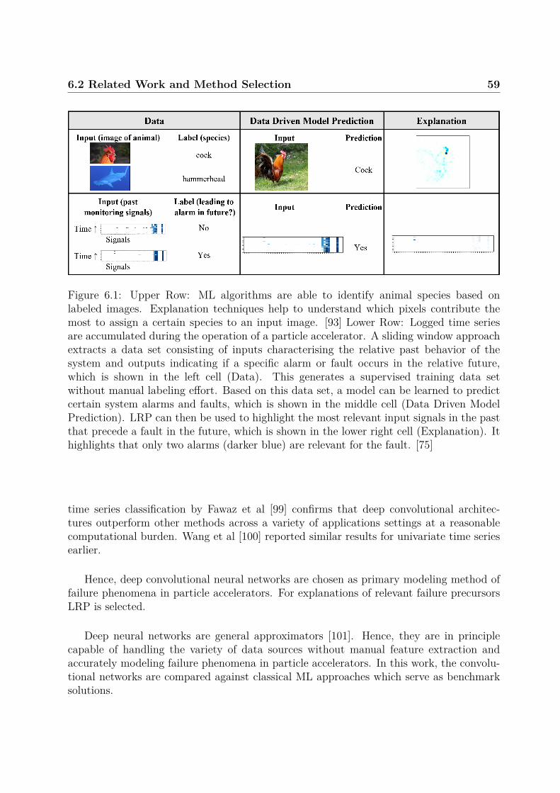
6.2 Related Work and Method Selection 59
Figure 6.1: Upper Row: ML algorithms are able to identify animal species based onlabeled images. Explanation techniques help to understand which pixels contribute themost to assign a certain species to an input image. [93] Lower Row: Logged time seriesare accumulated during the operation of a particle accelerator. A sliding window approachextracts a data set consisting of inputs characterising the relative past behavior of thesystem and outputs indicating if a specific alarm or fault occurs in the relative future,which is shown in the left cell (Data). This generates a supervised training data setwithout manual labeling effort. Based on this data set, a model can be learned to predictcertain system alarms and faults, which is shown in the middle cell (Data Driven ModelPrediction). LRP can then be used to highlight the most relevant input signals in the pastthat precede a fault in the future, which is shown in the lower right cell (Explanation). Ithighlights that only two alarms (darker blue) are relevant for the fault. [75]
time series classification by Fawaz et al [99] confirms that deep convolutional architec-tures outperform other methods across a variety of applications settings at a reasonablecomputational burden. Wang et al [100] reported similar results for univariate time seriesearlier.
Hence, deep convolutional neural networks are chosen as primary modeling method offailure phenomena in particle accelerators. For explanations of relevant failure precursorsLRP is selected.
Deep neural networks are general approximators [101]. Hence, they are in principlecapable of handling the variety of data sources without manual feature extraction andaccurately modeling failure phenomena in particle accelerators. In this work, the convolu-tional networks are compared against classical ML approaches which serve as benchmarksolutions.

60 6. Data-Driven Discovery of Failure Mechanisms
Proposed Approach
The proposed approach is illustrated in Figure 6.1. Logged time series are accumulatedduring the operation of a particle accelerator. These consist of fault, alarm or anomalysignals, and monitoring signals. A sliding window approach extracts a data set consistingof inputs characterising the (relative) past behavior of the system and outputs indicating ifa specific alarm or fault occurs in the (relative) future, which is shown in the lower left cellof the figure. This generates a supervised training data set without manual labeling effort.Based on this data set, a model can be learned to predict certain system alarms and faults,which is shown in the lower mid cell of the figure. LRP can then be used to highlight themost relevant input signals in the past that precede a fault in the future, which is shownin the lower right cell of the figure. It highlights that only two alarms (darker blue) arerelevant for the fault. With this information, system experts can focus their attention andfind solutions to arising reliability problems faster. The effective use of such a method canhelp to increase the availability of complex systems.
For example, certain magnet power converters steer particle beams based on feed-backfrom beam position monitors. Faulty beam position monitors could lead to noisy beamposition measurements which could trigger a preventive shut down of a power converter.This can lead to the interruption of operations of a whole particle accelerator.
A predictive method could forecast such a preventive shut down. However, withoutadditional information about the forecast, system experts have to manually search for thepotential root cause. Considering the sheer amount of possibly relevant signals, they mightnot identify the mechanism before the preventive shut down happens. However, LRP couldhighlight a faulty beam position monitor as the most relevant precursor, because its noisymeasurement disturbs the current regulation loop of the power converter. Based on thisautomatically generated hint, experts can simply replace the faulty beam position monitorand avoid an unplanned interruption of operations.
6.3 Methodology - Explainable Deep Learning Mod-els for Failure Mechanism Discovery
Definitions and Overview
An infrastructure composed of multiple sub-systems is studied. Its behavior is monitoredover time in a range of N observables, including event and alarm logs, continuous anddiscrete monitoring signals, and operational commands and settings. This forms a multi-variate time series, S = {Si,t : i ∈ [1 : N ] and t ∈ N}. The range of alarms, faults andanomalies, which should be predicted are contained within this range of observable signals.
A relation between (relative) past and future behavior of the infrastructure can beapproximated by an autoregressive model. It can only be approximated, since alarms andfailures may appear without any advance indicators (precursors). Even in situations withprecursors, they might not be captured by the monitoring systems. In a time discrete

6.3 Methodology - Explainable Deep Learning Models for Failure MechanismDiscovery 61
Figure 6.2: Time discrete model formulation. The x-axis represents discrete time andthe y-axis monitoring signals of the investigated infrastructure. Crosses mark events thatcould be faults, alarms, changes in monitoring values, etc. Events of the signal SN representinfrastructure faults that the model Φ(·) predicts. [75]
formulation, the approximate autoregressive model takes following form,
SFN,[t+tpδt : t+(tp+no)δt] ≈ Φ(SP[1:N ],[t−niδt : t])
with
• SFN,[t+tpδt : t+(tp+no)δt] = 1, if a failure occurs between time t+ tpδt and time t+ (tp +no)δt, and zero otherwise,
• SP[1:N ],[t−niδt : t] being finite histories of observed signals covering the time steps t−niδtto t and being considered as possible precursors,
• δt being the discretization time,
• tp the prediction- or lead-time,
• no the number of time steps chosen to capture the future failure behavior,
• ni the number of discrete time steps chosen to capture the history of the observedsignals and
• Φ an autoregressive model.
The model and its variables are illustrated in Figure 6.2. The x axis shows the discretizedtime and the y axis the various monitored signals.

62 6. Data-Driven Discovery of Failure Mechanisms
In all cases, except very simple systems, the autoregressive model Φ(·) cannot be ob-tained from first principles. Hence, the model is learned from observed historic data S, ac-cumulated during operations of the infrastructure. This is done in a supervised learning set-ting by providing pairs of input data, SP[1:N ],[t−niδt : t], and output data, SFN,[t+tpδt : t+(tp+no)δt].Different learning algorithms can be applied to the supervised training data set.
A trained model can predict the future system behavior if new observed input datais provided. However, it would predict the occurrence of a failure without the requiredinformation to prevent that failure. This required additional information is provided inthe form of a relevance measure, ρ(SP ) ∈ R(ni,N). It indicates the relevance of each inputsignal at each discrete time step. If a failure is predicted, the input signals contributingthe most to the prediction of a failure will be assigned the highest relevance values. Thisallows system operators and experts to focus their attention and remove failure conditionsbefore they lead to faults.
It has to be pointed out that the framework does not identify causal relations but onlytemporal precedence of correlated precursors of failures [102]. However, such informationhelps experts to establish causal models. Such findings can be integrated in model-drivensystem characterizations, such as presented in Chapter 7.
The methods can be used both in on- and offline analysis. As online tool, it acquiresdata from the infrastructure in real time as input and provides predictions and explanationsof imminent failures continuously. System operators can then use this information to carryout planned maintenance before the failures happen in an uncontrolled way. This requiresa lead-time, tp > 0, to give system experts sufficient time to react.
As offline tool, complex failure mechanisms that already occurred can be explainedusing the input activation function. System experts can then modify the infrastructure sothat the failure mechanism cannot occur again. As offline tool, no lead-time for predictionsis required.
ML Pipeline
In the following, the procedure to derive the autoregressive model Φ(·) from observed datais detailed. It consists of data collection, model selection and evaluation, subsamplingstrategies, input data filtering and normalization, training of models through learningalgorithms, and the explanation of their predictions. The procedure is summarized in apseudoalgorithm at the end of this section.
Data Collection Observable signals S from the investigated infrastructure are stored ina data-set D in time series format. The specific signals are selected so that the relevantfailure precursors and faults or alarms are contained in the data. Often this will be basedon expert recommendation. Further details of the data collection are provided in the usecase Section 6.5.
Model Selection and Evaluation The formulation of the autoregressive model includesa range of parameters, e.g. [δT, ni, no, tp] (some will be introduced later in this Section).

6.3 Methodology - Explainable Deep Learning Models for Failure MechanismDiscovery 63
These need to be optimized for the specific prediction task. This is carried out through anexhaustive grid search within a K-fold validation strategy [103]. Contrary to the widelyused cross-validation, the temporal order of the folds is never mixed. Instead, the trainingset is continuously expanded and the validation set shrunken.
Formally, the full data set, D, is split in a training set, Dtrain up to time tsplit, and afinal test set, Dtest after time tsplit. K further folds are obtained by splitting the training setinto sub-training sets and validation sets at subsequent split times tsub−split,k, k = 1, ..., K.
Subsampling In most cases, failures and alarms occur rarely in infrastructures. Hence,the output data SFN contains few failure examples (class ’1’) and many examples withoutfailures (class ’0’). This so-called class imbalance depends on the number of faults in thedata as well as the model formulation parameters, such as the discretization time δt or thenumber of time steps that capture failures no. For the considered use case, an imbalanceof up to 1 : 104 is observed. Such strong imbalances lead to difficulties when using thetraining algorithms. Hence, the classes need to be more balanced.
To achieve that, several sampling methods are applied. Random subsampling of themajority class (’0’) is applied until a pre-set target ratio, p0,targ = freq(cl0)/freq(cl1), isobtained.
Data items ncov time steps before and after each class ’1’ example are added as itincreases the ’contrast’ in the vicinity of class ’1’ occurrences. This leads to improvedclassification performance and can be considered as an upsampling strategy.
A choice of the output window length, no > 1, leads to no times oversampling of class ’1’items. This can result in an improved classification performance at the cost of a decreasedcertainty of the timing of predicted faults [76].
Input Filtering and Normalization Input signals, which do not contain statisticallysignificant information, are automatically removed. This includes input signals with lessthan αmin values non-equal to zero and signals with a variance smaller or equal to σmin.αmin = 4 is chosen as it represents the minimal number of data items from which any ofthe algorithms could discriminate a pattern[76]. σmin=0, is selected to remove constantsignals. All inputs are normalized to the range [0, 1].
Model Learning Algorithms Below, the different algorithms to learn the autoregres-sive model Φ(·) from observed data in a supervised fashion are discussed. The problem isa binary classification as the output variables can be either ’0’ or ’1’. Both deep learningand classical ML algorithms are used and compared.
Recent studies of deep learning for multivariate time series classification [99, 100] foundthat deep fully convolutional networks reach state of the art performance while being easierto train than recurrent neural networks. They are chosen as main modeling strategy andare compared against SVM, Random-Forest, and k-Nearest-Neighbor classifiers, which arechosen due to their past successes and wide usage. Each of the used algorithms is explainedin more detail below:

64 6. Data-Driven Discovery of Failure Mechanisms
• FCN: The architecture was proposed by Wang et al [100]. It is made of three blockswith three layers in each: a convolutional layer, a batch normalization layer [104], anda ReLU activation layer. A Global Average Pooling layer (GAP) averages the outputof the last block over the whole time dimension. The GAP layer is connected to asoftmax classifier. Each convolutional layer has a stride of one with zero padding forconservation of the input data shape. Each of the three convolutional layers contains128, 256, and 128 filters with a length of 8, 5, and 3, respectively. In comparison tothe implementation by Fawaz et al [99], the number of training epochs is set to 2000.The optimization is stopped earlier when the validation loss is not decreasing bymore than 0.001 within 200 epochs. The loss function is defined as categorical crossentropy. The model achieved the highest accuracy across 13 different multivariatetime series classification tasks in the study by Fawaz et al [99]. Hence, it was chosenas the main architecture.
• FCN2drop: Dropout regularization is recommended in situations with few trainingdata to avoid overfitting. It is expected to lead to a performance gain for the con-sidered scenario with very few class ’1’ data. The FCN architecture is taken withdropout applied to the second convolution layer and the GAP layer. The dropoutprobability is set to pdrop = 0.5.
• FCN3drop: The FCN architecture is taken with dropout applied to the second andthird convolution layer and the GAP layer. The dropout probability is set to pdrop =0.7.
• tCNN: Zhao et al [105] proposed a network consisting of two convolutional layerswith 6 and 12 filters each. A fully-connected layer with sigmoid activation functionconnects to it. The mean-squared error is used as loss function instead of cross-entropy. The same early stopping criterion as for FCN is added to the implementationof Fawaz et al [99].
• SVM: As reference classifier, a support vector machine with linear kernel functionsis used. The default implementation from the sklearn package [106] showed bestperformance across tasks and is used.
• RF: The random forest classifier is a meta classifier composed of multiple decisiontrees. The default sklearn implementation [106] is used. The parameter for theconsidered number of features for optimal splitting is changed to the square root ofnumbers of features.
• kNN: The k-Nearest-Neighbor classifier is used with default parameters from thesklearn package [106] except for selecting n = 7 neighbors.
Parameters for the classical methods (SVM, RF, kNN) were selected based on recommen-dations from the scikit-learn user guide [106] and a set of preliminary tests with datasimilar to those from the use case. Classical methods require one dimensional input data.

6.3 Methodology - Explainable Deep Learning Models for Failure MechanismDiscovery 65
This is achieved by flattening the 2D input data during training and predictions. Somespatial correlation information is lost during the flattening. The deep architectures do notsuffer from that as they can directly use the 2D data.
The performance of the classifiers is measured in terms of accuracy and F1 scores on thevalidation and test sets. The accuracy is reported together with the fraction of the majorityclass in the test data. This allows to assess if the classifier performs better than a trivialpredictor that always predicts the majority class. The F1 score is a suitable performancemetric for the class imbalance situation. Results are usually reported with the predictionlead-time tp as the time between fault prediction and actual fault influences the usefulnessof the prediction.
Explaining Predictions
The method quantifies the relevance of each input at each time step, ρ(SP ) ∈ R(ni,N),towards the classification output. This helps system experts identify the relevant failureprecursors. The input relevance is plotted in color maps. Darker colors signify higherrelevance.
LRP provides relevance measures for deep neural networks by propagating the classi-fication output backwards through the layers of a neural network. Neurons, which con-tribute more to a subsequent layer, pass back more relevance. This techniques achievesbest-in-class explanations [96]. A publicly available toolbox is used for implementation[107]. Different rules can be chosen. In preliminary tests, comparing Gradient x Input[95],LRP-0, and LRP-ε rules [93], LRP-0 demonstrated minimally better filtering of irrelevantfailure precursors.
For the SVM classifier the input relevance can be accessed through the input featureweight vector [106]. For kNN and RF the input relevance was not evaluated as they wereonly used as classification benchmarks.
The quality and usefulness of an explanation largely depends on the embedding ofthe method in actual usage settings. The overall explanation process can be assessed byevaluating user experience, e.g., as proposed by Holzinger et al [54].
Since the presented method is a proof of concept at the time of writing, such an assess-ment cannot be fully carried out. Instead, a simplified evaluation based on three criteria(derived from [54]) is used. The criteria are the completeness of the provided explanationfactors, the ease of understanding, and the degree of causality within the studied processesthat can be derived from the explanation [75]. They will be discussed for each of the ex-periments in Section 6.5. The timeliness of an explanation would be an interesting factoras well. However, without an actual online usage setting it cannot be estimated reliably.
6.3.1 PseudoalgorithmThe overall ML approach is summarized in by pseudoalgorithms below:
Pseudoalgorithm illustrating the overall process:
1. D load monitoring time-series data

66 6. Data-Driven Discovery of Failure Mechanisms
2. Split data D in training Dtrain and testing set Dtest
3. (Model selection:)For: varying parameters[p0,targ, ncov, δT, ni, no, tp, tsub−split] Do:
(a) Perform sub-algorithm (see below) ← [Dtrain, p0,targ, ncov, δT, ni, no, tp, tsub−split](b) Store obtained performance metrics Ptrain and input activation ρ(SP )train
on hold-out sets
4. (Model testing:)For: best performing model[p0,targ, ncov, δT, ni, no, tp, tsplit]optimal Do:
(a) Perform sub-algorithm ← [D, p0,targ, ncov, δT, ni, no, tp, tsplit]optimal(b) Store obtained performance metrics Ptest and input activations ρ(SP )test
on test set
5. Evaluate consistency between [Ptrain, ρ(SP )train] and [Ptest, ρ(SP )test] for optimalparameters
Sub-algorithm:1. Get parameters ← [D, p0,targ, ncov, δT, ni, no, tp, tsub−split]
2. Transform time series data to pairs of input data SP[1:N ],[t−niδt : t] and outputdata SFN,[t+tpδt : t+(tp+no)δt].
3. Split data in sub-training set(s), Dsub−train, and sub-testing set(s), Dsub−testat defined splitting time(s) tsub−split.
4. Perform sub-sampling on training set.
5. Perform input filtering and normalization
6. For: all target signals and classifiers Do:
(a) Train predictive model Φ(·) on Dsub−train(b) Evaluate performance metrics Psub−test and input activation ρ(SP )sub−test
on filtered and normalized sub-testing set
7. Collect and report performance metrics and input activation.
6.4 Data Requirements and AvailabilityThe data requirements of the proposed method and the actual availability of data are as-sessed. Since the method is developed for a scenario with limited a priori expert knowledgeon the system behavior, the data requirements focus on the available logged time series.

6.4 Data Requirements and Availability 67
Data Requirements The data can be distinguished in input data - time series charac-terising the ’past’ machine behavior - and output data - ’future’ events within the loggingtime series that should be predicted. There are no particular data format requirementsfor the input data as long as it can be encoded numerically. However, to achieve a goodpredictive performance, the input data should contain the relevant precursors for the futureevent to be predicted. The input data may also include past observations of the outputdata (i.e. if you want to predict future occurrences of alarm x, past occurrences of x maybe used as input).
The requirements for the output data are that the time series are discrete. In mostcases, failures are discrete binary events and automatically satisfy this condition. For themethod to show good performance there should be at least four examples of fault or alarmoccurrences in the data. This represents the absolute minimum for which the framework isable to detect patterns [76]. However, in that case the validation process relies on humanjudgement of the provided predictions and explanations. To carry out proper validationtechniques, such as cross-validation, faults or alarms should occur more than ten times inthe data. Generally, the more alarms are present in the data the more reliable the methodworks. When a specific alarm or fault signal represents a single failure mechanism, theinterpretation of failure explanations is simplified. However, the method does also workwhen different failure mechanisms are grouped into a single alarm signal.
Modifications of the studied infrastructure may introduce or remove certain failuremodes. If a method is trained on data lacking a failure mode, which is later introduced, itwill likely not be able to adapt its predictions. This is addressed by the chosen validationprocess to include the effects of infrastructure modifications for unbiased performanceestimates. Hence, changes in the infrastructure that may lead to predictive performancedegradation are discovered before the method is deployed to an operational setting.
Data Availability The actual data availability is assessed for the so-called Proton Syn-chrotron Booster (PSB) at CERN as introduced in Section 2.2.2. The method is laterapplied to this use case. The Monitoring and condition data, operational configurationsand settings, and failure and alarm data are continuously logged since 2014. Data betweenJanuary 2015 and December 2017 is selected for testing the method. It contained sufficientalarm data and the infrastructure did not substantially change within that time period.
For the input data, alarms, interlock, and beam destination signals are used. Thechoice was based on expert recommendation. They are expected to most likely containfailure precursors. However, the data logging systems were not designed for prognosticpurposes [108]. Hence, it can only be guaranteed that the input data satisfies the minimalrequirements. Whether failure precursors are actually present in the input data can beassessed with the explanation output provided by the proposed method.
For the output data, two power converter failure modes are considered: malfunction ofa power converter controller and failure of a current measurement device. Both occurredmore than ten times in the considered time frame. It is not known whether one or multiplefailure mechanisms lead to each of the failure modes. Again, it can only be guaranteed

68 6. Data-Driven Discovery of Failure Mechanisms
that the output data satisfies the minimal requirements.
Discussion Overall, the framework has very low minimal requirements for the data.If the data satisfies recommended requirements (precursors, number of fault occurrences,separate mechanisms), results are expected to be better and easier to interpret. Still,for data with minimal requirements the method should provide useful results. For theconsidered use case, the data availability and quality is acceptable but not optimal. Theresulting performance of the method for this case is discussed in detail in Section 6.5.
6.5 Numerical ExperimentsThe proposed approach is first validated on synthetically generated data and then testedon PSB particle accelerator data. Publicly available implementations are provided1.
6.5.1 Synthetic Data ExperimentsTo validate the approach it is applied to synthetically generated data. Using syntheticdata allows to assess if the framework predicts and identifies the manually created failuremechanisms correctly.
Noise Robustness The first experiment tests from how many input signals the correctfailure precursors can be isolated whilst fewer than ten failure examples are present. Forthis test, a infrastructure is simulated by nrand systems randomly firing alarms and onesystem Sp that produces two subsequent failure precursors which are followed by a criticalfailure of the infrastructure SFs . The pattern and its timing parameters are shown inFigure 6.3. The time evolves in the horizontal direction and the different signals are listedvertically. The Sp signal contains deterministic precursors. Two following signals causea fault signal SFs . A range of randomly activated noise signals, SR1 , SR2 , ..., representnon-relevant parts of the infrastructure.
The problem parameters are a time tbr ∼ N (µ = 14.61 d, σ = 14.61 d) between ran-domly firing precursors, SRl , l = 1, 2, ..., nrand, a time tbp ∼ N (µ = 1 d, σ = 1 d/24) be-tween deterministic precursors Sp, a time tpe ∼ N (µ = 10 d/24, σ = 1 d/24) between deter-ministic precursors Sp and infrastructure failures SFs , and a time tep ∼ N (µ = 36.525 d, σ =36.525 d) between infrastructure failure SFs and deterministic precursors Sp with d beinga day of 24 hours.[75] The data covers a time range of 2.7 years. nrand = [20, 21, ..., 29]randomly firing systems are added.
The method is applied with following parameters: Sampling times δt = [2 h, 3 h] (h forhours), input range ni = 40, lead-time tp = 0, output range no = [1, 2, 3, 4], sub-samplingtarget ratio p0,targ = 0.8, and class ’1’ neighborhood coverage ncov = 2. The data is split ata time tsplit so that 80 percent of the data-set are used for training and model-selection and
1https://github.com/lfelsber/alarmsMining

6.5 Numerical Experiments 69
Figure 6.3: Parameters of synthetic pattern. The Sp signal contains deterministic precur-sors. Two following signals cause a fault signal SFs . A range of randomly activated noisesignals, SR1 , SR2 , ..., represent non-relevant parts of the infrastructure. [75]
20 percent for final testing. A 7-fold validation is used for model selection. Sub-splittingtimes tsub−split are chosen to have [50, 55, 60, 65, 70, 75, 80] percent of training data and[50, 45, 40, 35, 30, 25, 20] percent for validation. Only 7 (13) critical failures were present inthe training data of the validation folds (the whole data-set) on average. This representsa realistic number of observed failures in historic data.
The results for δt = 3h and no = 2 are presented as with these hyper-parameters goodresults across classifiers are obtained. The F1 score and accuracy are plotted as a function ofthe number of randomly firing signals, nrand, in Figures 6.4a and 6.4b. For higher numbersof random signals the classification performance is decreasing for all classifiers. The FCN-based networks perform better overall. For up to fifty random signals, the patterns can bepredicted from only seven faults in the training data with an acceptable performance forthe FCN-based architectures.
Recovering Fault Tree Structure The second experiment tests whether faults due tointeractions of multiple sub-systems may be predicted and explained. For this experiment,data from two interacting sub-systems, SP1 and SP2 , and four additional non-interactingsub-systems, SR1−4 , are generated. An infrastructure fault, SFb , happens when simultaneousfailures of the two interacting sub-systems fulfill a Boolean AND, OR, or XOR condition.The parameters of the timing and delays of the signals are shown in Figure 6.5.
The data was generated with parameters tbr ∼ N (µ = 23 min, σ = 24 min) andtpe = 71 min, tep = 120 min. The framework is applied with following parameters:sampling time δt = 12 min (min for minutes), input range ni = 5, lead-time tp = 5,output range no = 1, sub-sampling target ratio p0,targ = 0.8, and class ’1’ neighborhoodcoverage ncov = 2. The data set is split in equally sized training and testing sets. No K-fold validation is performed, as no hyperparameters need to be selected in this case. Lessthan 20 critical failures are contained in the input data. Deep networks and traditionalmethods consistently reach F1 > 0.97. The explanation results for the FCN2drop networkare discussed in the following.
The input activations for the AND, OR, and XOR scenario are illustrated in Figure 6.6.The three lines represent three randomly selected system snapshots shortly before a critical

70 6. Data-Driven Discovery of Failure Mechanisms
(a) (b)
Figure 6.4: Dependency of the predictive performance on the number of randomly firingsignals. The line depicts the mean and the error bar plus and minus one standard deviationcalculated over the 7 validation sets. Solid lines represent deep models, which perform onaverage better than the classical models (dashed). (a) The F1 score. Note that the predic-tors level out at 0.0 for large nrand, which is the binary F1 score when always predictingthe majority class (’0’). (b) The accuracy. The predictors level out at 0.82 for large nrand,which is the accuracy when always predicting the majority class (’0’). [75]
Figure 6.5: Parameters of synthetic pattern. An infrastructure fault, SFb , happens whensimultaneous failures of the two interacting sub-systems, SP1 and SP2 , fulfill a BooleanAND, OR, or XOR condition. Four additional non-interacting sub-systems, SR1−4 , ran-domly trigger alarms that do not lead to a fault. [75]

6.5 Numerical Experiments 71
Figure 6.6: Illustration of AND, OR and XOR fault logic extraction. Left columns showthree randomly selected input windows before failure occurrence. Right columns show therelevant precursors obtained with the FCN2drop network (darker colors indicate higher rel-evance). Comparing the relevant precursors (right columns), allows to distinguish differentBoolean rules and recover the fault logic of the system. [75]

72 6. Data-Driven Discovery of Failure Mechanisms
error occurred. Left columns are the unfiltered input data and right columns show therelevant inputs after applying the LRP method. For all scenarios the relevant precursors,SP1 and SP2 , are correctly highlighted by the LRP method. By comparison of the differentsnapshots, the Boolean logic can be inferred successfully. However, this requires severalfault behaviors to be available at the same time.
The results confirm that different types of system interaction can be inferred from theexplanation output (left columns). The raw inputs (right columns) would not providesufficient information to do so. With respect to the proposed three criteria assessment,the explanation can be considered complete if several fault behaviors are observed. Fortwo interacting systems, the interaction mechanism is easy to understand. The degree ofcausality that can be derived from the explanation cannot be assessed for this syntheticexample.
Further synthetic data experiments with the proposed method have been carried outin [76]. Among the main findings are that an increase of no by one or two may improveaccuracy when the delay between precursors and faults exhibits high variance, that theinput relevance generally highlights precursors with lower timing variance stronger thansuch with higher variance, and that patterns can be identified from only four examples inextreme cases.
6.5.2 Particle Accelerator Data Experiments
In the following experiments, the method is applied to monitoring data sets (henceforthcalled ’real data’) from the PSB accelerator at CERN as described in the data availabilitySection 6.4. It is assessed whether the method can predict faults in advance from themonitored data and is able to extract relevant precursors, which explain the predictedfailure mechanisms.
As mentioned, the data set was not recorded for such data analysis purposes. It mostlyserved diagnostic purposes. Moreover, the infrastructures are continuously worked on.
The following data are taken for the analysis:
• Data of the LASER alarm database [109] contains logged alarms. They have a listof attributes including system name, fault code, and priority. For the chosen data,the priority take values 2 and 3. Priority 2 alarms are warnings, whereas priority 3alarms are faults leading to the shutdown of the affected system. An alarm beginswith a rising flag and ends with a falling flag. Only rising flags were used in theanalysis. Data from a group of eight power converters are chosen. For the input datarepresentation, all fault codes of a system were grouped. This results in eight inputsignals. The choice of target data is closer described in subsequent Sections.
• 27 Interlock signals were added based on expert recommendation. They record in-ternal and external disturbances, which can lead to an interruption of acceleratoroperation.

6.5 Numerical Experiments 73
Table 6.1: Performance metrics for mixing synthetic and real data experiments. fracmajstands for the fraction of the majority class and is shown as reference for the accuracy ofa trivial predictor always predicting the majority class. v and σv stand for the mean andstandard deviation over the 7 validation folds, respectively, and t for results on the testset. [75]
• The beam destination variable provides information on operational settings of theaccelerator. The eight beam destinations are one-hot-encoded and used as additionalinput data.
Overall, the data consists of 8 LASER alarm signals, 27 interlock signals, and 8 beamdestination signals. Time intervals in which the PSB is not operational are omitted, as thedata is not representing operational conditions.
Mixing Synthetic and Real Data In a preliminary step, it is tested if synthetic pat-terns can be isolated from the real world data. In that sense, the noise robustness experi-ment is repeated with the noise channels being replaced by the real world data describedabove.
The following framework parameters are used: sampling times δt = [2 h, 3 h] (h forhours), input range ni = 40, lead-time tp = 0, output range of no = [1, 2, 3, 4], sub-sampling target ratio p0,targ = 0.8, and class ’1’ neighborhood coverage ncov = 2. Themodel validation strategy is the same as for the noise robustness experiment.
Parameters δt = 3 h and no = 3 achieved high F1 scores and accuracy and are shownin Table 6.1. The columns indicate the different models that were trained. fracmaj standsfor the fraction of the majority class and is shown as reference for the accuracy of a trivialpredictor always predicting the majority class. v and σv stand for the mean and standarddeviation over the 7 validation folds, respectively, and t for results on the test set. Thelines show the F1 (denoted F1_cl1) and the accuracy (denoted acc).
Only 7 faults are present in the training data. Despite that, the FCN network achievesan F1 score close to 1. This indicates that a well defined failure pattern in real data couldbe detected by the FCN network from less than ten training examples.
The input activation plots for the FCN network and the SVM are presented in Fig-ure 6.7a. Both methods correctly identify the synthetic precursors from the 45 signals. Interms of the three assessment criteria of the quality of explanations, they can be consideredcomplete and easy to understand. The causality cannot be assessed for the synthetic case.
Real Data As final test, the method is applied to the real data set. It is tested whetherit can predict and explain two types of power converter alarms with priority 3: fault code
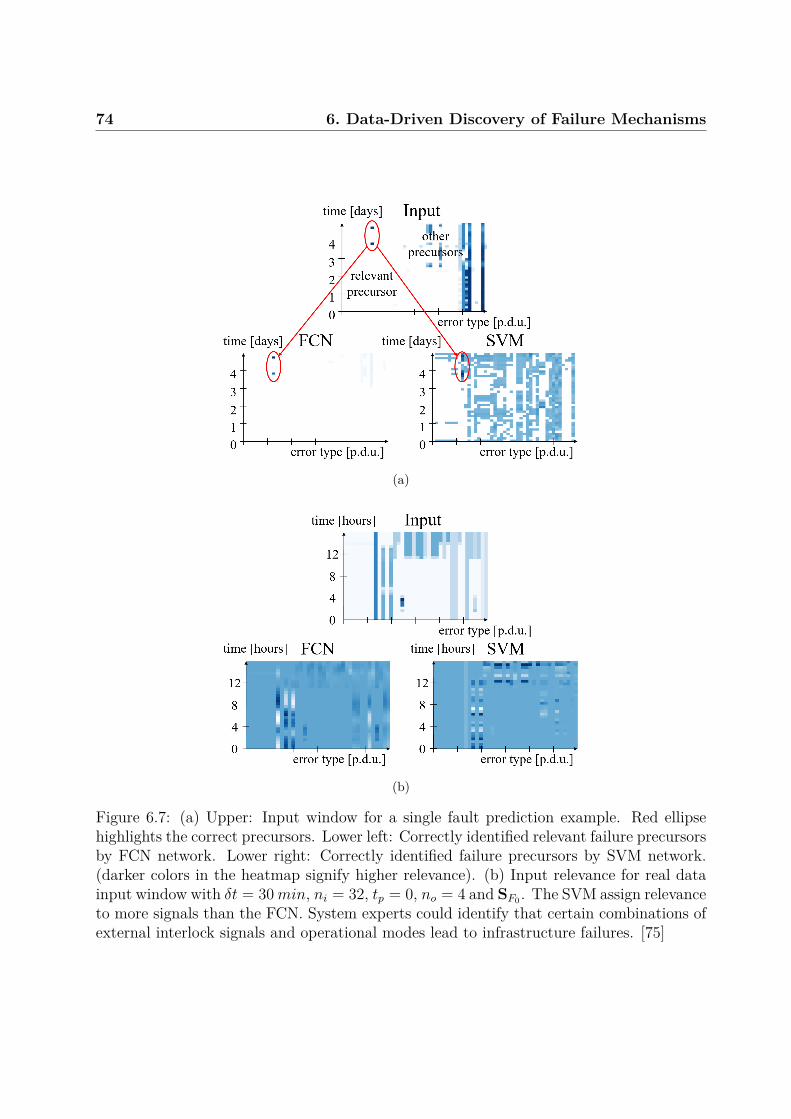
74 6. Data-Driven Discovery of Failure Mechanisms
(a)
(b)
Figure 6.7: (a) Upper: Input window for a single fault prediction example. Red ellipsehighlights the correct precursors. Lower left: Correctly identified relevant failure precursorsby FCN network. Lower right: Correctly identified failure precursors by SVM network.(darker colors in the heatmap signify higher relevance). (b) Input relevance for real datainput window with δt = 30min, ni = 32, tp = 0, no = 4 and SF0 . The SVM assign relevanceto more signals than the FCN. System experts could identify that certain combinations ofexternal interlock signals and operational modes lead to infrastructure failures. [75]
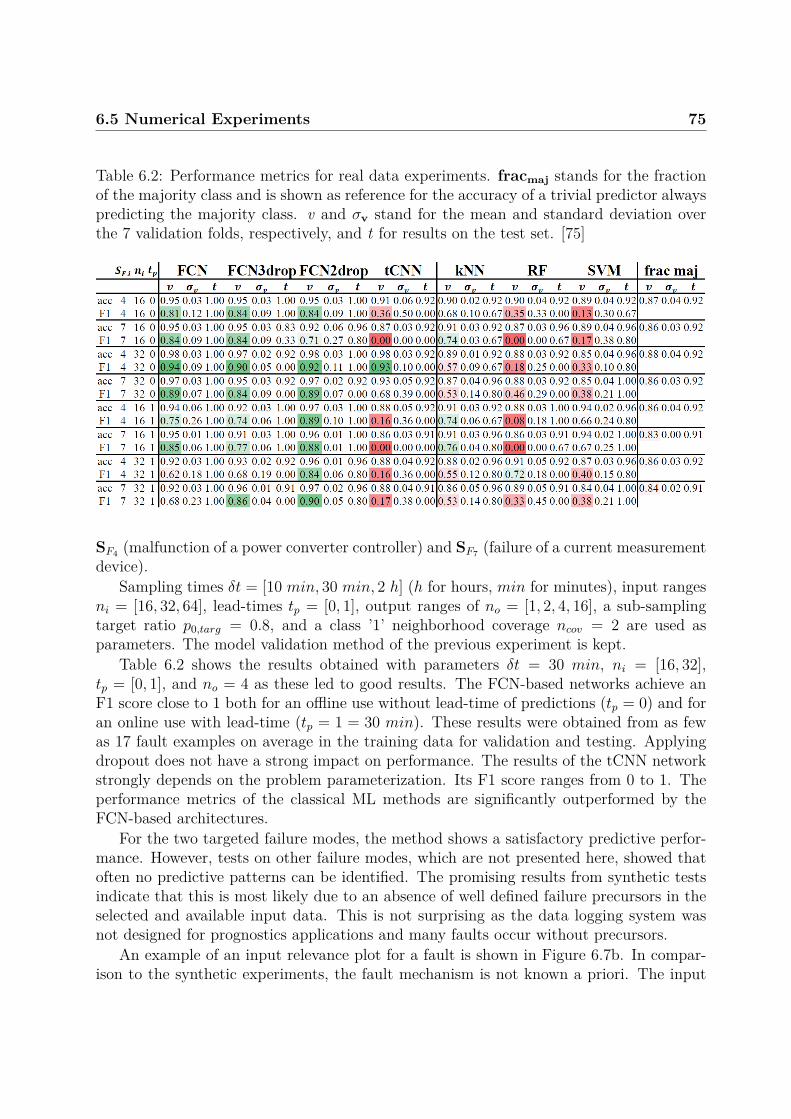
6.5 Numerical Experiments 75
Table 6.2: Performance metrics for real data experiments. fracmaj stands for the fractionof the majority class and is shown as reference for the accuracy of a trivial predictor alwayspredicting the majority class. v and σv stand for the mean and standard deviation overthe 7 validation folds, respectively, and t for results on the test set. [75]
SF4 (malfunction of a power converter controller) and SF7 (failure of a current measurementdevice).
Sampling times δt = [10 min, 30 min, 2 h] (h for hours, min for minutes), input rangesni = [16, 32, 64], lead-times tp = [0, 1], output ranges of no = [1, 2, 4, 16], a sub-samplingtarget ratio p0,targ = 0.8, and a class ’1’ neighborhood coverage ncov = 2 are used asparameters. The model validation method of the previous experiment is kept.
Table 6.2 shows the results obtained with parameters δt = 30 min, ni = [16, 32],tp = [0, 1], and no = 4 as these led to good results. The FCN-based networks achieve anF1 score close to 1 both for an offline use without lead-time of predictions (tp = 0) and foran online use with lead-time (tp = 1 = 30 min). These results were obtained from as fewas 17 fault examples on average in the training data for validation and testing. Applyingdropout does not have a strong impact on performance. The results of the tCNN networkstrongly depends on the problem parameterization. Its F1 score ranges from 0 to 1. Theperformance metrics of the classical ML methods are significantly outperformed by theFCN-based architectures.
For the two targeted failure modes, the method shows a satisfactory predictive perfor-mance. However, tests on other failure modes, which are not presented here, showed thatoften no predictive patterns can be identified. The promising results from synthetic testsindicate that this is most likely due to an absence of well defined failure precursors in theselected and available input data. This is not surprising as the data logging system wasnot designed for prognostics applications and many faults occur without precursors.
An example of an input relevance plot for a fault is shown in Figure 6.7b. In compar-ison to the synthetic experiments, the fault mechanism is not known a priori. The input
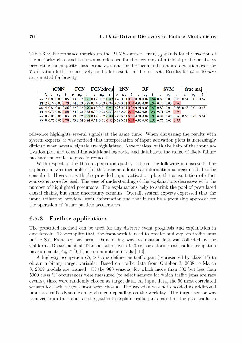
76 6. Data-Driven Discovery of Failure Mechanisms
Table 6.3: Performance metrics on the PEMS dataset. fracmaj stands for the fraction ofthe majority class and is shown as reference for the accuracy of a trivial predictor alwayspredicting the majority class. v and σv stand for the mean and standard deviation over the7 validation folds, respectively, and t for results on the test set. Results for δt = 10 minare omitted for brevity.
relevance highlights several signals at the same time. When discussing the results withsystem experts, it was noticed that interpretation of input activation plots is increasinglydifficult when several signals are highlighted. Nevertheless, with the help of the input ac-tivation plot and consulting additional logbooks and databases, the range of likely failuremechanisms could be greatly reduced.
With respect to the three explanation quality criteria, the following is observed: Theexplanation was incomplete for this case as additional information sources needed to beconsulted. However, with the provided input activation plots the consultation of othersources is more focused. The ease of understanding of the explanations decreases with thenumber of highlighted precursors. The explanations help to shrink the pool of postulatedcausal chains, but some uncertainty remains. Overall, system experts expressed that theinput activation provides useful information and that it can be a promising approach forthe operation of future particle accelerators.
6.5.3 Further applicationsThe presented method can be used for any discrete event prognosis and explanation inany domain. To exemplify that, the framework is used to predict and explain traffic jamsin the San Francisco bay area. Data on highway occupation data was collected by theCalifornia Department of Transportation with 963 sensors storing car traffic occupationmeasurements, Oh ∈ [0, 1], in ten minute intervals [110].
A highway occupation Oh > 0.5 is defined as traffic jam (represented by class ’1’) toobtain a binary target variable. Based on traffic data from October 3, 2008 to March3, 2009 models are trained. Of the 963 sensors, for which more than 300 but less than5000 class ’1’ occurrences were measured (to select sensors for which traffic jams are rareevents), three were randomly chosen as target data. As input data, the 50 most correlatedsensors for each target sensor were chosen. The weekday was hot encoded as additionalinput as traffic dynamics may change depending on the weekday. The target sensor wasremoved from the input, as the goal is to explain traffic jams based on the past traffic in

6.6 Chapter Summary, Conclusions and Outlook 77
other locations.The framework is applied to the data with sampling times δt = [10 min, 30 min], an
input range ni = 10, lead-times tp = [0, 1, 2, 4, 8], an output range of no = [1, 2, 3], asub-sampling target ratio p0,targ = 0.5, and a class ’1’ neighborhood coverage ncov = 2.The same model validation strategy is chosen as for the synthetic data experiment. Allclassifiers were trained and evaluated.
In Table 6.3, the results are shown for traffic sensor 401390 which is located on theGrove Snaffer Fwy in Oakland (coordinates 37.827454, -122.267769). Note that traffic jamsare predicted with F1 scores close to 1 up to four hours in advance. In this experimentwith continuous, numeric data, the RF, FCN and FCN2drop classifiers show the bestperformance. The successful application of our modelling approach to an application froma completely different domain gives confidence in the general validity of the results obtainedin previous experiments and underlines the universality of the employed methods.
6.6 Chapter Summary, Conclusions and OutlookA framework to identify and predict failure mechanisms for situations with limited a pri-ori knowledge on the system behavior is presented. It can handle data sets encounteredin realistic settings, such as in particle accelerators, containing multivariate signals, rawdata of heterogeneous types, and few observed failures. It uses deep convolutional neuralnetworks to extract predictive failure patterns from historic monitoring data. This allowsprediction of faults in real time.
To help system experts and operators interpret the predictions, the most relevant failureprecursors are highlighted by Layer wise Relevance Propagation (LRP). Thereby, reactiontimes to arising problems can be shortened and recurring failure conditions can be removed.This has the potential to improve the availability of future particle accelerators.
The method is validated on synthetic data. It can correctly identify predictive patternsfrom as few as seven examples for up to 50 input signals. The type of interactions betweenmultiple systems that lead to failures can be reconstructed with the explanations providedby the method.
For data from the PSB accelerator at CERN, the framework predicts power converterfaults with F1 scores close to 1. It can do so at a bare minimum of data preprocessing,from fewer than 20 failure examples, and without manual labeling effort of the data. Thefailure explanations help system experts to narrow the pool of potential failure causes andspeed up troubleshooting. The results are encouraging because the historical data of theuse case was not collected for predictive purposes. Modern systems collect increasinglymore monitoring signals containing failure precursors. This facilitates the application ofthe introduced method further.
The following research could increase the effectiveness of the proposed approach further:
• Few shot and transfer learning approaches might learn predictive failure patternsfrom even fewer failure examples.

78 6. Data-Driven Discovery of Failure Mechanisms
• Complex infrastructures are evolving systems. Re-learning schemes allow to updatepredictive models continuously. This renders the approach fit for the long term usageof such a method in evolving infrastructures.
• Using logarithmic time scales on the input data could capture failures happeningover particularly long time scales, such as wear-out phenomena.
The method is generally useful to predict and explain discrete events in time series. Forapplications outside the particle accelerator domain, it only needs adaption of the input-and output data provision and the grid of optimization parameters. Potential examplesinclude identifying root causes of stock market crashes, climate phenomena, or transmis-sion of diseases. Within the field of reliability studies, the method has demonstrated to beuseful for the operation of complex particle accelerators and, hence, can be a promisingtool for other complex systems.
Chapter Learning Summary
Explainable Deep Learning can help improve the operations of particle accelerators.This requires that fault data as well as data that might contain fault precursors arelogged during operation. Data logging objectives should be expanded from explainingfaults that occurred to hinting at faults that will occur.

Chapter 7
Data and Knowledge-DrivenParametric Model-Based ReliabilityOptimization
In the previous chapter the modeling was mainly data-driven as expert and knowledge-based models of the studied system were hardly available. Contrary to the previous chapter,below a scenario is studied in which a priori knowledge on the failure behavior of a systemis already available. Such knowledge could be the output of classical reliability analysiscarried out by system experts.
In such scenarios information is available in both quantitative (e.g. fault time distribu-tion) and qualitative (expert knowledge on causes of faults) form. This requires flexible,data-effective modeling strategies capable of exploiting all available knowledge. Purelydata-driven methods, such as in the previous chapter, are ineffective in encoding quali-tative expert knowledge as their model structure is not flexible enough and their modelparameters do not directly translate into a physical meaning. A parametric modeling strat-egy can include both quantitative and qualitative knowledge effectively and transparently.Hence, they are better suited for such scenarios.
Below, such a parametric reliability modeling strategy including a simulation concept ispresented, which addresses RQ2. Each of its modules is based on well established reliabilityconcepts which allows translation to and from expert knowledge. This also has the benefitto assess whether such models can predict system behavior under novel operating conditionsand even for re-designed systems. In combination with the simulation engine, optimaldesigns, operational strategies, and maintenance schedules with minimal life cycle cost,can be determined.
The methods, findings and some of the illustrations of this chapter have been publishedpreviously in [111, 112].
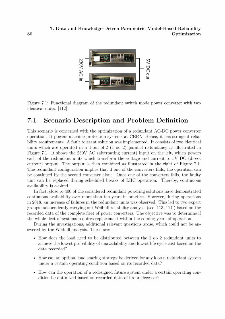
807. Data and Knowledge-Driven Parametric Model-Based Reliability
Optimization
5V
DC
ou
t
230
V A
C in
Figure 7.1: Functional diagram of the redundant switch mode power converter with twoidentical units. [112]
7.1 Scenario Description and Problem DefinitionThis scenario is concerned with the optimization of a redundant AC-DC power converteroperation. It powers machine protection systems at CERN. Hence, it has stringent relia-bility requirements. A fault tolerant solution was implemented. It consists of two identicalunits which are operated in a 1-out-of-2 (1 oo 2) parallel redundancy as illustrated inFigure 7.1. It shows the 230V AC (alternating current) input on the left, which powerseach of the redundant units which transform the voltage and current to 5V DC (directcurrent) output. The output is then combined as illustrated in the right of Figure 7.1.The redundant configuration implies that if one of the converters fails, the operation canbe continued by the second converter alone. Once one of the converters fails, the faultyunit can be replaced during scheduled breaks of LHC operation. Thereby, continuousavailability is aspired.
In fact, close to 400 of the considered redundant powering solutions have demonstratedcontinuous availability over more than ten years in practice. However, during operationsin 2018, an increase of failures in the redundant units was observed. This led to two expertgroups independently carrying out Weibull reliability analysis (see [113, 114]) based on therecorded data of the complete fleet of power converters. The objective was to determine ifthe whole fleet of systems requires replacement within the coming years of operation.
During the investigations, additional relevant questions arose, which could not be an-swered by the Weibull analysis. These are:
• How does the load need to be distributed between the 1 oo 2 redundant units toachieve the lowest probability of unavailability and lowest life cycle cost based on thedata recorded?
• How can an optimal load sharing strategy be derived for any k oo n redundant systemunder a certain operating condition based on its recorded data?
• How can the operation of a redesigned future system under a certain operating con-dition be optimized based on recorded data of its predecessor?

7.2 Related Work and Methods Selection 81
Optimization
of operation Digital
Reliability
Twin
100 SystemsOperating Condition
500 SystemsOperating Condition
20 SystemsAccelerated Testing
Failure and
operations data
Future SystemsOperating Condition
Optimization
Existing systems Future Systems
Figure 7.2: Overview of the approach. Data from a system operating at different conditionsis combined to form a digital reliability twin, which can be used to optimize existing andfuture systems under different operating conditions. [112]
In this chapter, a generic approach is developed to address these questions based on thedata availability for the power converter example. The approach to address these questionsis illustrated in Figure 7.2: A transparent reliability model (Digital Reliability Twin in thecenter of Figure 7.2) is learned with data and knowledge from existing systems in differentoperating conditions (on the left in Figure 7.2). Then, the model can be used to optimizenew operational scenarios of existing and future systems (on the right in Figure 7.2).
The metric for these optimizations is the life cycle cost Equation 3.11. The equipmentcost is the cost of the (redundant) power converter, the repair cost is the cost of replacingone of the redundant units, and the downtime cost is the cost due to interruption of theoperation of the powered system. As for all reliability optimization techniques, the earlieravailable in the system life cycle and the more precise the results are, the bigger is theirpotential value for decision making. Moreover, due to the scarcity of operational failures,the method has to be suitable for small data regimes. Hence, the developed approachshould be data-effective and able to handle uncertainties due to limited data.
7.2 Related Work and Methods SelectionThis section discusses the relevant work for the considered approach. These are the digitaltwin framework and degradation models of load-sharing systems.
Digital Twins The desired objective requires an approach, which integrates data col-lection, data analysis, modeling, simulation, and cost assessment. A framework, whichcombines all these steps is the digital twin.
The term digital twin has been coined by Glaessgen et al [115]. They describe it as’an integrated multi-physics, multi-scale, probabilistic simulation of a complex product

827. Data and Knowledge-Driven Parametric Model-Based Reliability
Optimization
and uses the best available physical models, sensor updates, etc., to mirror the life of itscorresponding twin...’. With respect to reliability, they note that ’the digital twin willincrease the reliability of the [system] because of its ability to continuously monitor andmitigate degradation and anomalous event’. This means that they perceive a prognosticssolution to increase the system reliability using the digital twin approach.
The limitations of existing prognostics solutions have been discussed in Chapter 4.These include lack of appropriate data and models to predict system behavior accurately.As the digital twin would rely on such models to increase system reliability, it suffers fromthe same limitations.
Documented implementations of the digital twin paradigm for reliability purposes arescarce. Tuegel et al [116] and Cerrone et al [117] show how existing methods can be ex-tended with ideas of the digital twin in the aeronautics industry. Reifsnider et al [118] pro-pose a digital twin-based method for composite materials. Gabor et al [119] and Alaswadet al [120] discuss implementation options and potential advantages of digital twins.
Despite the practical implementation challenges of the digital twin, its integrated datacollection, modeling and simulation concept is appealing. It aims at coherence between thedata collection, usage and the desired decision objectives - similar to the project assessmentstage (see Section 5.2) used for implementations of methods in this thesis.
To overcome the disparity between the proposed high fidelity modeling and high reso-lution sensor updates and the actual availability of reliability models and data in variousfields of industries, a more conservative modeling approach can be a first useful step. Meth-ods based on accelerated testing, such as pioneered by Nelson [121, 122, 123], are moreappropriate for the data availability considered in this and many other realistic scenarios.They can be combined with a simulation engine and a cost model to achieve cost-effectivereliability optimization.
Load Sharing Degradation Analysis and Modeling In the following, relevant exist-ing work in terms of reliability analysis and modeling of load-sharing systems are discussedas it forms the core of a digital twin approach for the considered scenario.
The main challenge in modeling the load sharing of redundant systems is that the loadsand stresses within the redundant units are interdependent. A failure in one of the unitsinfluences the loads of all other units. Hence, even for applications with constant loads,the load profiles within redundant units are dynamic. Several methods have been proposedto model such dependencies and are discussed below.
Early modeling approaches were limited to exponential failure rates (constant hazardrate) and 1 oo 2 systems, due to a lack of detailed reliability models and insufficientcomputational performance [124]. Such modeling is too inaccurate to be useful in realisticsettings. In such models, the failure probability of the system does only depend on its ageand instantaneous load. However, empirical studies showed that the entire load history isrelevant for determining the instantaneous failure rate [125, 126, 123].
Over time, more accurate modeling approaches based on the Weibull failure distribution(non-constant failure rates) and the cumulative exposure model [121] were developed [127]

7.3 Methodology - Parametric Digital Reliability Twins 83
for 1 oo 2 systems. Such approaches consider the load history.More recently, efficient computational procedures to extend such modeling to large k
oo n systems have been produced [128]. Multiple failure modes within redundant unitswere modeled by Huang et al [129]. Modeling approaches which allow the incorporationof qualitative knowledge about the failure mechanism have been proposed by Yang et al[130]. Some methods even consider specific behaviors of redundant units, such as delaysdue to rebooting [131].
Despite the many variations of reliability modeling of load sharing systems, no approachfor a combination of non-constant hazard rates, handling the effect of load histories on mul-tiple failure modes, non-balanced load sharing, and propagation of parametric uncertaintyhas been reported so far. However, these are requirements to model the considered powerconverters scenario realistically.
Since most presented approaches are based on methods of accelerated life testing [121,123], the existing modeling approaches can be extended to arrive at the desired modeling.Combined with a simulation approach and the cost model, as suggested by the digital twinapproach, the objectives outlined in the previous section can be addressed. The detailswill be explained in the next Section.
7.3 Methodology - Parametric Digital Reliability Twins
7.3.1 Overview
The overview of the proposed methodology is given in Figure 7.2. A quantification ofsystem reliability, here called Digital Reliability Twin (in the center of the figure), is learnedfrom existing system under different operating conditions (in the left of the figure) usingmethods from Accelerated Life Testing (ALT). The models can be continuously updated,once new data is generated during operations. The model can be used to optimize theoperation of existing and future systems in new operating conditions (in the right of thefigure).
The execution of the approach is based on four steps. These are data collection, digitaltwin synthesis, simulation, and evaluation and decision making. These steps will be carriedout for a use case in Section 7.4.
Below, the elements of the Digital Reliability Twin are introduced. Firstly, the quan-titative model behind the Digital Reliability Twin and the required reliability modelingbackgrounds and definitions are presented. After that, a Monte Carlo engine to simulatethe system over its life cycle is discussed. Then, the cost model for life cycle cost evaluationand decision making is introduced. Finally, the data collection requirements and actualdata availability and quality is assessed.

847. Data and Knowledge-Driven Parametric Model-Based Reliability
Optimization
U1
I O
E
U2
Um
ID OC
Figure 7.3: Redundant system illustration.
7.3.2 Reliability Modeling of Load Sharing in Redundant Sys-tems
The quantitative model of the Digital Reliability Twin and the required reliability modelingbackgrounds and definitions are presented as follows:
1. The relevant definitions for redundant systems are introduced.
2. The modeling of multiple failure modes by Weibull distributions is discussed.
3. The acceleration factor modeling is outlined to describe the effect of system loads onstresses or failure drivers.
4. The cumulative exposure model is introduced to describe degradation under variablestresses.
5. The load sharing of multiple redundant units is discussed.
6. All the previous modeling steps are combined into a hierarchical load sharing model.
7. The hierarchical load sharing model is validated on a benchmark problem from theliterature.
8. A summary of the modeling approach is provided.
Definitions Figure 7.3 illustrates a redundant system S. It is composed of an InputDistributor (ID), Output Collector (OC), and n redundant identical units, U1, .., Un. Asystem boundary (dashed line) separates it from an operational environment E. Theoperating conditions are referred to as the collection of environment, input and output,C = [E, I,O]. The system is considered available, if it delivers the specified output Owhilst the environment and the input are within specifications. It is faulty if it fails to doso.

7.3 Methodology - Parametric Digital Reliability Twins 85
Multiple Failure Modes in Redundant Units A failure in a k oo n redundant systemoccurs when more than k−n units are simultaneously in a failed state, the input distributoris faulty, or the output collector has a failure. In the considered scenarios, the inputdistributor an the output collector are extremely simple and robust designs. Hence, theyare assumed to have no failures.
The reliability of a single Unit Ui at a time t is described by its reliability function,Ri(t). Its probability of being faulty at time t is given by Fi(t) = 1 − Ri(t). Differentfailure mechanisms j may lead to the failure of a unit. They are modeled as competingrisks [37], Fi(t) = 1−∏M
j=1(1− Fj).The failure probability due to a single failure mechanism can be modeled by several
statistical models [8, 6]. The two parameter Weibull distribution is chosen as it is fre-quently used in reliability studies and commonly known by system experts. It is givenby, Fj(t; ηj, βj) = 1 − e(−t/ηj)βj , t > 0. ηj is the characteristic lifetime (with the propertyFj(t = ηj) ≈ 0.63212) and βj is the shape parameter that indicates a decreasing (βj < 1),constant (βj = 1), or increasing (βj > 1) failure rate with time for a failure mechanism j.
Acceleration Factor Modeling A failure mechanism is activated by a failure driver,ξj. For example, increasing temperature leads to a faster evaporation of the electrolytein capacitors. This degrades its capacity. For this example, the failure driver is thetemperature and the failure mode is capacity degradation. The stress ξj results fromsystem operating conditions, C. Their relation can be expressed by empiric or analyticmodels, ξj = Γj(C; Λ), with parameters Λ. For the capacitor case, such a model wouldexpress the capacitor temperature as a function of the operating current, which causes heatdissipation.
Acceleration factor modeling allows to quantify the relationship between the failuredriver and the time to failure. With a two-parameter Weibull distribution, the accelerationfactor is expressed as, AFj(ξj, ξj,ref ; Θ) = ηj,ref/ηj. ηj,ref is the characteristic lifetimeat a reference operating condition1, ξj,ref = Γj(Cref ). Parameters Θ define the kind ofacceleration model. The acceleration factor model is often expressed by exponential- orpower-laws, e.g. AFj(ξj, ξj,ref ; Θ) = (ξj/ξj,ref )Θ. [49, 112]
Cumulative Exposure Model To consider the degradation of the redundant units dueto their non-stationary load history, the cumulative exposure model is used [121]. It isbased on acceleration factor modeling by summing the load history dependent accelerationfactor over time: AF (ξstress(t), ξref ) . Thereby, an effective system age τ is obtained,
τ(t) =∫ t
t′=0AF (ξstress(t′), ξref ) dt′. (7.1)
A system with a failure probability characterized by a two parameter Weibull distributionunder reference conditions, tfail,ref ∼ Weibull(ηref , βref ), will fail once the effective system
1Note that we assume uniform acceleration, i.e. βj,ref = βj . The methodology can be extended tonon-uniform acceleration. However, a changing βj indicates a changing failure mode and should be dividedin separate failure modes.

867. Data and Knowledge-Driven Parametric Model-Based Reliability
Optimization
Figure 7.4: Illustration of the proposed hierarchical load-sharing modeling strategy.
age exceeds the the reference failure time drawn from the Weibull distribution, τ(T ) >tfail,ref . Thereby, the effect of arbitrary load histories can be assessed when the systemfailure probability under a reference operating condition, as well as its acceleration factormodel, are known.
Load Sharing Modeling So far, a relationship between the failure probability of theredundant units and its operating conditions has been established. The missing pieceis the relation between the system load L and its influence on the operating conditions.Specifically, the load on each of the redundant units, Li, has to be determined as a functionof the system load and the available redundant units. This is modeled by so-called loadsharing policies, Li = LSPi(L), which distribute the system load among the functionalredundant units. A very common load sharing strategy is balanced load sharing, which isalso used for the power converter example. Two other sharing strategies are studied: Hot-Spare operation, in which some of the units are in stand-by mode without any load, andimbalanced load sharing, in which the load is distributed unequally among the functionalunits.
For the considered 1 oo 2 scenario, LSP1:1 stands for balanced load sharing with halfof the load on each unit, LSP1:0 for hot spare operation with the whole load on one unit,and LSP1:2 with one third of the load in one unit and two thirds of the load on the otherunit.
Hierarchical Load Sharing Model A combination of all the introduced concepts in ahierarchical way leads to a modeling approach to support the decision objectives for theconsidered scenario. Figure 7.4 shows the resulting hierarchical modeling approach. Thesystem load L is the relevant operating condition at the highest modeling level. A loadsharing policy LSP distributes the system load among the redundant units. A parametricmodel Γ determines the stress ξ for failure mode j on unit i as a function of the unit loadLi. The stress ξi,j determines the acceleration of the degradation through the accelerationfactor AFi,j. Finally, the failure time of the unit is determined through the cumulativeexposure model and its Weibull failure probability at reference load. Combining all ex-

7.3 Methodology - Parametric Digital Reliability Twins 87
0.0 0.5 1.0 1.5 2.0 2.5Time t [au]
0
1
2
[au] Load L2
Acceleration factor AFFailure stressor
(a)
0.0 0.5 1.0 1.5 2.0 2.5Time t [au]
0.0
0.5
1.0
F i(t) Simulation
Load on single unitLoad shared
(b)
Figure 7.5: Application of the proposed load-sharing and the cumulative exposure model[121] to a 1 oo 2 redundant device: (a) Simulation parameters over time. (b) Illustrationof the failure probabilities for unit two over time. The blue dashed line corresponds to thesimulated failure probability for the described scenario. The green and red line depictsthe failure probability for half or full system load, respectively. Note the increasing failurerate at tc = 0.7. The time difference between the green and red line can be evaluatedanalytically as ts = tc(1− 1/AF (L0.5, (L/2)0.5) [132]. [111]
pressions, the failure probability for a unit can be expressed as
F (t,C; ηj,ref , βj,Λ,Θ) =
1−M∏j=1
1− exp(−∫ t
0 AFj(Γj(C(t′); Λ), ξj,ref ; Θ)dt′ηj,ref
)βj . (7.2)
Model Validation The validity of the model is assessed by reproducing the results ofvariable load failure behavior as reported by Pozsgai et al [132]. It concerns a 1 oo 2redundant system with a single failure mode, tfail,ref ∼ Weibull(ηref = 1, βref = 1.5), apower-law acceleration factor, AF (ξstress, ξref ) = (ξstress/ξref )1.6, a nonlinear load-stressorrelationship, ξi,stress = L0.5
i , and a balanced load-sharing policy, L1 = L2 = L/2. Theoperation of unit 2 is simulated from time t = 0 to t = 4. At time tc = 0.7, unit 1 is shutdown. Hence, for t > tc unit 2 supports the full load. The resulting load, accelerationfactor, and stress profile (y axis) for unit 2 are shown as a function of time (x axis) inFigure 7.5a. The discontinuity of the profiles occurs at tc = 0.7, when unit 1 is shut down.
The simulation is carried out by drawing reference failure times, tfail,ref ∼ Weibull(ηref =1, βref = 1.5), from the Weibull distribution above. The unit operates until the effectiveage τ exceeds the drawn reference failure time, τ(t) > tfail,ref . The effective age is cal-culated by the cumulative exposure model under the given load. By recording the time tfor repeated experiments, the cumulative failure probability F2(t) under the variable loadcan be determined. The resulting cumulative fault distribution under the variable load(dashed line) is shown in Figure 7.5b together with the cumulative failure probabilitieswhen assuming the two constant load settings (red and green lines). The first constantload setting assumes a shared load up to tc = 0.7. Thereafter, the second load setting

887. Data and Knowledge-Driven Parametric Model-Based Reliability
Optimization
assumes that all the load is on a single unit. The cumulative fault distribution under thevariable load follows the failure probability of the shared load setting up to tc = 0.7 andcontinues along the failure probability of the single unit setting thereafter. The results areidentical to those of Pozsgai et al [132], which validates the chosen modeling approach.
Model Summary Despite its overall complexity, the hierarchical model is composed ofsimple layers of widely used functions in reliability studies. This has the advantage thatsystem experts are more likely to be familiar with it and their knowledge can be translatedinto parameter values. When their knowledge is not sufficient, parameters can be obtainedby consulting scientific literature in which these functions are often used. Finally, theparameters can also be obtained from system failure data through parameter estimationtechniques.
For the common situation of partial knowledge of parameter values, it is even possibleto mix expert knowledge, related scientific work, and operational data. E.g., in a Bayesianparameter inference scheme, prior distributions on parameter values can be determinedwith experts and posterior estimates obtained from the available data. This ensures thatall available data is used effectively.
Since the operating conditions are explicitly modeled, it is possible to study the systembehavior for new operating conditions as long as the acceleration factor and load to stressrelationship is valid. Thereby, the operation of the system can be optimized for newoperational environments.
As the fault mechanisms are modeled separately, it can be assessed how redesigns ofthe system affect reliability. Failure modes can be removed or modified individually if aredesign affects them. This allows to optimize the operation of redesigns of existing systemsto a certain extent. Moreover, the model addresses the requirements of a combination ofnon-constant hazard rates, handling the effect of load histories on multiple failure modes,and non-balanced load sharing. The propagation of distribution parameter uncertainty iscovered by using an appropriate simulation strategy, which is explained in the followingsection.
7.3.3 Simulation EngineThe presented hierarchical model allows to determine the failure time of a redundant unitas a function of the system load history. To determine the optimal operational policy ofthe system, a simulation engine needs to be added. It consists of the following elements:
• Core Model: It simulates the operation of a single system S stochastically for a life-time, which includes faults, repairs and the load sharing strategy. The correspondingstate diagram for a redundant system, such as the power converter, is shown in Fig-ure 7.6. It contains two system states, ’Operation’ and ’Down’, which indicate ifthe overall system is available or not. The simulation starts by drawing lifetimes ti,jfrom the Weibull distributions for each unit i and each failure mechanism j. Whilstin ’Operation’, the simulated time t is evolving and damage is accumulated through

7.3 Methodology - Parametric Digital Reliability Twins 89
Start SimulationIf Then:
• Terminate simulation
If Failure on any unit with any failure mode Then:
• Log fault details and times
• Set state of unit as “faulty
• Draw repair time • Start repair on unit
If Critical failure (leading to loss of output)Then:
• Log fault details and times
• Draw critical repair time • Start critical repair
If Critical failure repair finished Then:
• Log downtime spent in critical repair
• Set all repaired units as “operational”
• Draw reference lifetimes for all
repaired units and their affected failure
modes
If Repair on any unit finished Then:
• Set state of unit as “operational”
• Draw new lifetimes for
repaired unit and all failure modes
affected by repair
System
parameters
System
variables
Unit
parameters
Unit
variables
Operation
E: Loss of
Output
Down
E: Critical repair
finished
Figure 7.6: Illustration of the core level simulation approach: Simulation parameters aredefined as inputs for the simulation; Simulation variables are written during run-time ofthe simulation; (Middle): State diagram of the proposed simulation strategy and the statetransition conditions. [111]
the system loads as specified in the hierarchical model. Once a unit p fails due to amechanism q, a repair is initiated. It is finished after a repair time tr,q, which is drawnfrom a repair time distribution Tr,q. During the repair, the load on the remainingfunctional units is distributed according to the specific load sharing policy LSP . Ifn − k − 1 (i.e. a critical amount of) additional units fail before unit p is repaired,the system stops ’Operation’ and goes into the ’Down’ mode. This initiates a criticalrepair with a duration tr,c ∼ Tr,c. Once the critical repair is finished, the systemreturns to the ’Operation’ state. The simulation terminates when the simulated timeexceeds the operational lifetime of the system, t > TOL. After the simulation hasfinished, all faults and fault times, repairs, and downtime events are reported.
• Core Initializer: The presented hierarchical model is stochastic. That means thata single evaluation of the model would be a sample of a random variable. To geta more complete characterization of the model behavior, many evaluations need tobe obtained to observe the distribution of the random variable. The Core Initializerexecutes many such evaluations of the core model with the same initialization param-eters. The results of all simulations can be expressed as distributions and statisticsthereof (e.g. the mean and variance). The required number of evaluations for sucha Monte Carlo-based simulation can be estimated by monitoring the convergence ofstatistics of the reported distributions.
• UQ Initializer: The modeling and simulation parameters are often uncertain due tolimited data and knowledge. To perform an end-to-end uncertainty-quantification,the Core Initializer is executed multiple times with model and simulation parame-

907. Data and Knowledge-Driven Parametric Model-Based Reliability
Optimization
Dependency Initializer
UQ Initializer
Core Initializer
Core model
Figure 7.7: Layered simulation approach. [112]
ters drawn from their respective distributions. As before, the number of necessaryexecutions can be determined by monitoring the statistics of the results.
• Dependency Initializer: The last layer allows to study the influence of different opera-tional parameter combinations to assess the influence of different operational strate-gies. E.g. different load sharing policies, different loads, or different maintenancestrategies can be compared.
The overall simulation approach, consisting of the four layers described above, is illustratedin Figure 7.7. The outer layers pass parameters P to the inner layers, whereas the innerlayers report simulation results R to the outer layers.
7.3.4 Cost ModelBased on the simulation results (or their statistics), the life cycle cost can be evaluatedusing equation 7.3,
C = neqceq + nrcr + ndcd, (7.3)
with nr being the number of repairs, nd being the number of downtime events duringthe system lifetime, and neq the equipment cost factor to consider additional costs due toredundancy. For the specific optimization objective, the equipment cost ceq is not relevantas it does not change depending on the chosen load sharing policy. Hence, it will be omittedhere. The number of repairs and downtime events are provided by the simulation. Therepair and downtime cost need to be determined for the considered use case. This will bediscussed in the following section.

7.3 Methodology - Parametric Digital Reliability Twins 91
7.3.5 Data Requirements and AvailabilityThe data assessment is carried out by first stating the data requirements for the proposedmodeling approach. Then the requirements are cross-checked with the actually availabledata.
Data Requirements The envisaged modeling consists of three elements:
1. the hierarchical system failure behavior quantification,
2. the simulation over a system life cycle, and
3. the life cycle cost equation.
The hierarchical model itself is composed of a load sharing policy LSP , a relationship Γbetween unit load Li and failure mechanism stress ξi,j with parameters Λ, an accelerationfactor model AF relating between a reference stress ξref and the actual stress, and atwo parameter Weibull distribution characterizing the unit failure probability over time atreference stress for each failure mode j.2
The simulation model requires a parameterized hierarchical model and a system oper-ation parameters. These are the operational lifetime TOL, repair time (distributions) Tr,critical repair time (distributions) Tr,c, the system load L(t), other operating conditionsC(t) (temperature, humidity, etc.), and the configuration of the redundant system (k oon).
Finally, the cost model is based on knowledge of the (average) repair and downtimecost. The cost of the equipment is not relevant in the considered optimization setting.
Data Availability Based on the outlined data requirements, the feasibility of the pro-posed modeling approach will be evaluated by assessing the actual data availability andquality.
The parameters of the hierarchical model are taken from expert reliability analysis onoperational data from more than ten years, totaling 58 Mu-h (Mega unit-hours). The datahas been recorded by a system expert who has been in charge for the whole operationalperiod. The data is well documented and consistent [113]. Two independently carriedout investigations on the data identified the same Weibull parametrization of the failurebehavior [114]. The acceleration model parameters and the load-stress relationship modelwere developed in additional studies [133, 114] which were presented to expert panels.Therefore, the data availability and quality can be considered sufficient. The only limitationis that it was noted that due to the limited data availability, the parameter estimates arerather uncertain. However, no systematic uncertainty-quantification was performed so far.To address this issue, an ad-hoc sensitivity analysis is performed by assuming that the
2When limited knowledge about the specific load-stress relationship is available, it can be skipped bysetting Γ = Li.

927. Data and Knowledge-Driven Parametric Model-Based Reliability
Optimization
0 2 4Unit Current [A]
0
20
40
60
C8
Tem
pera
ture
[C]
exponential fitmeasured points
Figure 7.8: Experimentally determined relationship between temperature and load on unitξj(Li) = T (I). [112]
parameters follow normal distributions with a mean given by the expert-estimated valuesand a variance of 10% of their mean.
Many of the required simulation parameters are provided in the expert reliability anal-ysis [114, 113]. Only the repair time distributions needed to be gathered separately. Thiscould be done by interviewing the responsible expert for the repair of the system. Therepair costs were taken from the expert analysis.
It was noticed that the data collection is simplified by the availability and projectparticipation of the system designer and system maintainer. Moreover, during systemdesign a structured data collection procedure was implemented already. It facilitates thecoherent collection of data.
Overall, the available data satisfies the requirements for method implementation. Nev-ertheless, the results are interpreted with caution, as the uncertainty of the parameters isnot estimated systematically. In the following Section, the implementation of the proposedapproach and its results for the considered redundant power converter are presented.
7.4 Numerical ExperimentsIn this Section, the implementation of the described methods and its results for the usecase are presented.
The redundant powering solution is composed of two identical 1 oo 2 redundant switchmode power converters as shown in Figure 7.1. The converters have been operated at theLHC for more than 10 years during which 59 faults have been recorded. For each fault, fail-ure times ti,j, modes j, and operating conditions C are known [113]. The n = (290, 45, 58)systems have been operated at constant loads of L = (0.4, 0.9, 1.2)A, respectively. Theinput voltage is 230 V AC and the output voltage is 5 V DC.
The reliability investigations [113, 114, 133] identified three failure modes and theirassociated Weibull distributions and acceleration factor model. These are summarized in
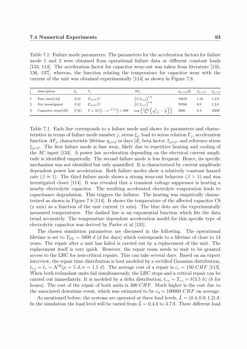
7.4 Numerical Experiments 93
Table 7.1: Failure mode parameters: The parameters for the acceleration factors for failuremode 1 and 2 were obtained from operational failure data at different constant loads[133, 114]. The acceleration factor for capacitor wear-out was taken from literature [135,136, 137], whereas, the function relating the temperature for capacitor wear with thecurrent of the unit was obtained experimentally [114] as shown in Figure 7.8.
j Description ξj Γj AFj ηj,ref [d] βj,ref ξj,ref
1 Fuse wear[134] I[A] Punit/U(I/Iref
)1.019219 1.16 1.2A
2 Not investigated I[A] Punit/U(I/Iref
)0.676768 0.9 1.2A
3 Capacitor wear[135] T [K] T = 55(1− e−0.7I
)+ 298 exp
(0.94kb
(1
Tref− 1T
))4200 8.3 330K
Table 7.1. Each line corresponds to a failure mode and shows its parameters and charac-teristics in terms of failure mode number j, stress ξj, load to stress relation Γj, accelerationfunction AFj, characteristic lifetime ηj,ref in days [d], beta factor βj,ref , and reference stressξj,ref . The first failure mode is fuse wear, likely due to repetitive heating and cooling ofthe AC input [134]. A power law acceleration depending on the electrical current ampli-tude is identified empirically. The second failure mode is less frequent. Hence, its specificmechanism was not identified but only quantified. It is characterized by current amplitudedependent power law acceleration. Both failure modes show a relatively constant hazardrate (β ≈ 1). The third failure mode shows a strong wear-out behavior (β > 1) and wasinvestigated closer [114]. It was revealed that a transient voltage suppressor is heating anearby electrolytic capacitor. The resulting accelerated electrolyte evaporation leads tocapacitance degradation. This triggers the failures. The heating was empirically charac-terized as shown in Figure 7.8 [114]. It shows the temperature of the affected capacitor C8(y axis) as a function of the unit current (x axis). The blue dots are the experimentallymeasured temperatures. The dashed line is an exponential function which fits the datatrend accurately. The temperature dependent acceleration model for this specific type ofelectrolytic capacitor was derived by Parler et al [135].
The chosen simulation parameters are discussed in the following. The operationallifetime is set to TOL = 5000 d (d for days) which corresponds to a lifetime of close to 14years. The repair after a unit has failed is carried out by a replacement of the unit. Thereplacement itself is very quick. However, the repair team needs to wait to be grantedaccess to the LHC for non-critical repairs. This can take several days. Based on an expertinterview, the repair time distribution is best modeled by a rectified Gaussian distribution,tr,j = tr ∼ NR(µ = 5 d, σ = 1.5 d). The average cost of a repair is cr = 150 CHF [113].When both redundant units fail simultaneously, the LHC stops and a critical repair can becarried out immediately. It is modeled by a delta distribution, tr,c ∼ Tr,c = δ(3.5 h) (h forhours). The cost of the repair of both units is 300 CHF . Much higher is the cost due tothe associated downtime event, which was estimated to be cd = 100000 CHF on average.
As mentioned before, the systems are operated at three load levels, L = (0.4, 0.9, 1.2)A.In the simulation the load level will be varied from L = 0.4A to 3.7A. Three different load

947. Data and Knowledge-Driven Parametric Model-Based Reliability
Optimization
sharing policies are studied: balanced load sharing LSP1:1, hot-spare operation LSP1:0,and imbalanced load sharing LSP1:2. Depending on the parameter combination, up to107 evaluations of the Core Model have been executed to obtain stable estimates of thenumber of repairs and downtime statistics. Hundred evaluations were carried out on theCore Initializer Level for robust estimates of the uncertainty bounds.
Results The simulated life cycle cost (y axis) as a function of the load sharing policy(balanced load sharing LSP1:1 in red, hot-spare operation LSP1:0 in green, and imbalancedload sharing LSP1:2 in blue) and the system output current (x axis) is shown in Figure 7.9a.The dashed line represents the mean. The shaded area shows the 95% highest probabilitydensity interval. The expected mean of the number of repairs and the number of downtimeevents recorded during the simulation are shown in Figure 7.9b with dash-dotted andsolid lines, respectively. Again, the shaded area shows the 95% highest probability densityinterval. The cost is a linear combination of the the number of repairs and downtimeoccurrences. Due to the cost discrepancy of a factor of thousand between the repair andthe downtime costs, the number of downtime events dominates the overall cost.
Evidently, the system behavior changes with output load. For low currents (I < 1 A),the cost is similar for all load sharing policies. For intermediate currents (1 A < I < 2.5 A),balanced load sharing has the lowest cost and hot spare operation results in the highestcost. For high currents (2.7 A < I), balanced load sharing has the highest cost andimbalanced operation results in the lowest cost. Currents, 2.5 A < I < 2.7 A, are in atransition period for which the cost of balance load sharing rapidly increases relative tothe other load sharing policies.
Figure 7.9c gives further insight in the frequency of the different failure modes in theimbalanced load sharing scenario. The expected number of failures for each failure modeand unit (y axis) is plotted as a function of the system output current (x axis). Failuremodes 1 to 3 are represented by different colors. Generally, the first unit (solid lines), whichcarries two thirds of the load, has a higher number of failures than the second unit (dashedlines), which only carries one third of the load. Failure modes one and two increase steadilywith the output load. Failure mode three is negligible for low currents but dominant forhigh currents.
Discussion The system shows non-trivial failure behavior. Depending on the outputload, different load sharing policies are cheaper in terms of life cycle cost. Balanced loadsharing leads to lowest costs in low and intermediate current scenarios, whereas for highercurrents it results in the highest costs. To explain the behavior it helps to remember thatthe third failure mode (capacitor wear) has a very strong wear-out behavior while the firsttwo failure modes are constant (random) in time. The third failure mode is dominantfor high currents. Hence, with higher currents, the units develop a stronger wear-outcharacteristic. This means that if the load is shared equally among the units, there is ahigher chance of simultaneous wear-out and failure, which leads to a downtime event. Ifthe load is not shared equally (or not at all), simultaneous wear-out is much less likely.

7.4 Numerical Experiments 95
0.5 1.0 1.5 2.0 2.5 3.0 3.5System output current [A]
101
102
103
104
Cos
t [C
HF]
cLSP1 : 1
cLSP1 : 0
cLSP1 : 2
(a)
0.5 1.0 1.5 2.0 2.5 3.0 3.5System output current [A]
10 5
10 4
10 3
10 2
10 1
100
101
Exp
. num
ber
of o
ccur
ence
s
nr 1:1nr 1:0nr 1:2nd 1:1nd 1:0nd 1:2
(b)
0.5 1.0 1.5 2.0 2.5 3.0 3.5System output current [A]
10 7
10 5
10 3
10 1
Exp
. num
ber
of o
ccur
ence
s
nr 1:2 (sum)fm1 u1fm1 u2fm2 u1fm2 u2fm3 u1fm3 u2
(c)
Figure 7.9: Final simulation results; Lines represent the expected means and shaded areasthe 95% highest probability density intervals: (a) The system cost C in CHF for differentload-sharing policies at different system loads (currents). (b) The total number of repairsnr, and the number of losses of system output nd for different load-sharing policies atdifferent system loads (currents). (c) The expected number of failures per failure mode forthe LSP1:2 load-sharing scenario; ’fmx uy’ stands for failure mode x on unit y.

967. Data and Knowledge-Driven Parametric Model-Based Reliability
Optimization
That is the explanation for the higher number of downtime events for the balanced loadsharing strategy for increased system loads. Such a behavior could only be identified dueto the detailed modeling of the failure modes, their mechanisms, and the dynamic loadsharing. In a purely data-driven analysis without separation of failure mechanisms, suchinsights would have been overlooked easily.
The width of the 95% intervals is determined by the parameter uncertainty and thestochastic nature of the problem. The contribution of the stochasticity could be reducedby increasing the number of system evaluations. Due to the low probability of simultane-ous failures in the two units for low output loads the statistics of the results are uncertaindespite up to 107 Monte Carlo evaluations. The contribution of the uncertain input param-eters is due to ad-hoc assumption of their uncertainty based on expert judgement. Hence,the actual uncertainty bounds might differ.
Decision Recommendation The original decision objective was to determine the op-timal load sharing policy for the power converter system. Based on the simulation results,it is concluded that the optimal load sharing strongly depends on the output load. For thethree operational currents, I = (0.4, 0.9, 2.4)A, balanced load sharing seems to result in thelowest cost. However, for high currents it might develop into a costly solution. Imbalancedload sharing seems to offer a low cost for all currents. Hence, considering the parametricuncertainty and the limited data, the safest strategy is imbalanced load sharing.
7.4.1 Further ApplicationsAs initially suggested in Figure 7.2, the parameterized model of a single unit can be usedto optimize operations of the existing system under new operating conditions or even forredesigned systems. In the example above, the objective was to optimize operations ofthe existing system. In a follow-up work [112], the same model has been used to optimizethe operation of a future system. The use of a single power converter unit in a non-redundant manner was studied for a less critical application with lower downtime cost. Theobjective was to determine the optimal maintenance strategy. The conclusion was that forlow currents, reactive maintenance leads to lower life cycle costs. For higher currents, apreventive maintenance is advisable. The optimal timing of preventive replacements couldalso be determined for different output loads.
Re-designs of the units could be assessed as well. E.g., it could be decided to usedifferent fuses. Then, the models for the second and third failure mode could be recycled.Potential new failure modes due to the different fuse would have to be identified separately.
If the whole system failure behavior was encoded in a neural network instead of theproposed hierarchical model, it would be very complex, if not impossible, to assess whichparameters of the models can be reused if the associated system is re-designed. Further-more, the parametric hierarchical model allows to derive more generally applicable insightsinto system degradation. An example is that it could be identified that the optimal loadsharing for redundant units depends on their hazard rate characteristics. This illustratesthe advantage of a transparent parametric modeling approach.

7.5 Chapter Summary, Conclusions and Outlook 97
7.5 Chapter Summary, Conclusions and OutlookA parametric modeling approach for reliability optimization projects with mixed availabil-ity of qualitative and quantitative data has been presented. At its core is a hierarchicalmodel composed of relatively simple and commonly used reliability models, such as theWeibull and acceleration factor model. This modeling approach allows to infer model pa-rameters in a combined manner from expert knowledge, scientific literature, and directlyfrom data. The hierarchical model is combined with a simulation engine and a life cyclecost model. It allows to study the system behavior under previously unseen operatingconditions and assessment of the reliability of future redesigns of the system.
The proposed method has been applied to a redundant powering solution to determinethe load distribution among the redundant units with the lowest life cycle cost. The resultsshow that the optimal load sharing solution depends on the output load, which influencesthe hazard rate characteristics. Balanced load sharing has low costs for low output load.For high output currents, balanced load sharing leads to the highest costs as the unitshave a higher risk of simultaneous failure. This may result in high downtime costs. Theimbalanced load sharing results in low costs for all operating loads. Hence, based on thelimited certainty of available data and knowledge, it is recommended as the safest loadsharing policy.
The parametric hierarchical modeling strategy demonstrated to be useful in settings ofmixed qualitative and quantitative information. The same system degradation model canbe used to optimize systems and system derivations under current and future operatingconditions. Such optimizations would be less effectively carried out with purely data-drivenmodeling strategies.
Chapter Learning Summary
Expert knowledge and fault data can be combined to improve reliability models.Such models can be used to improve system operation for new operating conditionsand redesigned systems.

987. Data and Knowledge-Driven Parametric Model-Based Reliability
Optimization

Chapter 8
Data-Driven Discovery ofOrganizational Reliability Aspects
The previous two chapters concerned scenarios with a focus on technical aspects of reliabil-ity. Chapter 6 aims at discovering fault mechanisms and using them to predict imminentfailures. Chapter 7 provided a systematic way to combine expert knowledge and data todevelop quantification of failure behavior under different operational settings. Both chap-ters use information of the system when in an operational state, encoded either in data,documentation, or expert knowledge. To improve the reliability of the systems, suitabletechnical modifications, e.g. optimal component choice or design, can be derived from theresults of applying the methods.
However, the reliability of a system is also affected by aspects such as project manage-ment, outsourcing of fabrication, or level of experience of the involved project stakeholders.The methods in the previous chapters do not provide information on the relevance of suchaspects for system reliability.
This chapter introduces a method to address such aspects to address RQ3. Based onthe field reliability of systems and relevant information of their life cycle, a multivariateparametric model is derived and subsequently trained. It can be used to predict thereliability of future fielded systems and extract the most relevant factors influencing it.This information allows effective organizational decision making early in a system lifecycle, which maximizes cost-effective reliability improvement.
This Chapter and the methods and results therein are based on previously publishedwork [138].
8.1 Scenario Description and Problem DefinitionIt is desirable to be able to predict the reliability of a system in advance to check whetherthey are expected to fulfill the specified reliability requirements, compare design alterna-tives, determine the required amount of spares, or calculate expected warranty cost.
The reliability of a system in the field is influenced during all phases of its life cycle.

100 8. Data-Driven Discovery of Organizational Reliability Aspects
All technical, human, and organizational processes may have a positive or negative impacton the system reliability. E.g., particle accelerators can take decades from the first ideato their operation. They will be conceived, designed, built, tested, commissioned andoperated by generations of engineers with diverse backgrounds. The tasks of each of themmay influence the achieved performance of the accelerator during operation.
Modeling of all these processes is impractical. Instead, common reliability predictionmethods restrict the modeling to limited aspects of a system (e.g. design, componentchoice) or phases during the life cycle (e.g. manufacturing, testing). A summary of existingmethods is provided in Section 8.2. Since these methods only model certain aspects, theirreliability predictions may be misleading, if the modeled aspects do not contain otherrelevant aspects within a system life cycle. Moreover, they cannot provide a systematicway to quantify the uncertainty of their predictions since potentially important life cycleaspects are not considered.
To overcome this limitation, a statistical model of field reliability is learned for thewhole system life cycle based on data from existing comparable systems as illustrated inFigure 8.1. So-called quantitative reliability indicators are collected for a group of existingsystems (grey box). When their field reliability is known (green box), multivariate regres-sion can be used to establish a relation (orange box) between the quantitative reliabilityindicators and the achieved field reliability. Such a model allows to predict the field relia-bility of new systems and to identify the relevant factors during a system life cycle. Usingappropriate regression methods, the uncertainty of predictions and influencing factors canbe quantified.
To measure the predictive performance of the methods common regression metricscan be used. They can be compared against the error of traditional reliability predictionmethods. Few studies have systematically evaluated the discrepancy between predictedand actual reliability of systems. Jones et al [139] conclude that reliability predictions candeviate by orders of magnitude between different traditional methods and the actual fieldreliability. These errors emerge because the used methods model the reliability based on theselection of components and ignore other relevant aspects, such as design considerations,manufacturing, or supplier selection.
Such imprecise reliability predictions may even mislead design choices. Hence, relia-bility prediction has to be considered highly stochastic and difficult and an uncertaintyquantification is essential for such problems.
In this chapter, a reliability prediction use case of power converters in particle acceler-ators is studied. It is shown that with the proposed approach the field reliability can bepredicted accurately with few reliability indicators, which are available early in a systemlife cycle. This allows to use the approach early in a system life cycle when it is poten-tially most valuable. The workload is greatly reduced in comparison to other reliabilityprediction methods, as the modeling does not need to be carried out manually becauseit is automatically inferred from the available data. With appropriately chosen reliabilityindicators and regression methods, the influence of each reliability indicator is quantified.It is shown that non-technical factors show a strong impact on the field reliability. Suchinformation can help improving reliability cost-effectively on an organizational level.

8.2 Related Work and Methods Selection 101
1) Conceptual Design
2) Detailed Design and
Testing
3) Manufacturing
4) Installation5) Operation
and Maintenance
a) Quantitiative
Reliability Indicatorsb) ML model c) Field Reliability
Figure 8.1: Illustration of the proposed approach. The achieved field-reliability (c) can beseen as the result of relevant processes during the whole product life cycle (1-5). It is notfeasible to capture and model all of the relevant processes. Instead, it is proposed to learna reduced-order statistical life cycle model (b) with machine-learning algorithms based onquantitative reliability indicators (a). [138]
8.2 Related Work and Methods SelectionReliability predictions have evolved over recent decades [140]. IEEE standard 1413 andits successors give an overview over the numerous existing approaches towards reliabilityprediction [141, 142]. The standard proposes a classification by
• handbooks,
• stress and damage models (also called physics-of-failure-based), and
• field data.
These groups of methods are discussed in the following.
Handbook-Based Methods Handbook methods use catalogued reliability data forcomponents to form a reliability estimate. A major criticism is that they do not con-sider interactions between components and their configuration but only fault frequenciesof single components. Numerous studies have found that single-component failures onlymake up for a fraction of failures in the field [143, 140, 144, 145, 146]. This leads to devi-ations between predicted and actual field reliability by orders of magnitude [139]. Densonet al argue that handbook based methods should only be taken as preliminary estimatesfor early life cycle stage design choices.
Stress and Damage Model-Based Methods Stress and damage models yield moreaccurate reliability estimates than handbook based methods [147]. They are based onan understanding of the failure mechanisms in a system and how they are influenced by

102 8. Data-Driven Discovery of Organizational Reliability Aspects
operational conditions. The method and use case from Chapter 7 are an example of a stress-and damage model. Although superior in the predictive performance, model generationrequires much more modeling and data collection effort.
Field Data-Based Methods Methods based on field data estimate the reliability of afuture system based on experience with similar systems and a similarity metric [148, 149].Their performance mostly depends on the method to derive the similarity metric and theavailability of reliability data of similar systems. The method proposed in this chaptercould be seen as field data-based, whereas it derives the similarity metric automaticallyfrom the available data.
Miller et al [150] evaluate the likelihood of a system achieving a target reliability byreviewing its design process. They determine a score depending on the design steps carriedout and show that it correlates with the probability of achieving the reliability target.This allows to include organizational aspects. The method proposed in this chapter takesa similar approach except that it directly estimates the expected reliability and identifiesthe most appropriate scoring method from the data.
Groen et al [151] developed a Bayesian framework to predict reliability of new systemsbased on similar systems and expert judgement. Their framework quantifies predictiveuncertainty. However, it involves an iterative approach with manual data input which isdependent on expert judgement. The proposed method of this Chapter does not requiremanual input beyond data collection as it infers all relevant dependencies from the supplieddata.
The studies of Miller et al [150] and Groen et al [151] demonstrate that reliability canbe forecasted accurately with methods based on field data. The proposed approach extendsthese methods by automatically extracting significant factors that influence the reliabilityfrom the data, quantifying uncertainty of reliability predictions and its influencing factors,and being able to include all potentially relevant aspects during a system life cycle. It isdescribed in detail in the following section.
8.3 Methodology - Statistical System Life Cycle Mod-els
This section introduces relevant definitions, the mathematical formulation of the problem,the data collection, the model selection process, and the model learning algorithms.
8.3.1 DefinitionsSystem Reliability Measure The method aims to predict a metric which expressesthe reliability of the system. E.g., this can be a reliability function or the remaining usefullife. For this scenario, repairable systems are considered. Therefore, we use the availabilityA as reliability measure as defined in Equation 3.7 based on the MTBF and MTTR. The

8.3 Methodology - Statistical System Life Cycle Models 103
MTBF is calculated byMTBF = toperation
nfaults, (8.1)
with toperation being the cumulative operational time of the considered repairable systemand nfaults being the total number of faults within the operational time. The MTTR isevaluated by
MTTR = tinrepairnfaults
, (8.2)
with tinrepair being the total time a system is in repair and nfaults the total number of faultsduring the operational time.
System Definition In this scenario, the considered systems are power converters ofmagnets in particle accelerators. The method is not restricted to certain types of systemsas long as they can be assigned a reliability measure and a life cycle.
8.3.2 ApproachThe method assumes that the achieved field reliability of a system is the result of allthe processes in all phases of the system life cycle. Statistical models approximate therelation between all relevant processes and the achieved field reliability. The statisticalmodels learn this approximation from observed reliability data and reliability indicatorsthat describe the life cycle of a fleet of comparable systems. Inspection of the generatedmodels allows to identify the most relevant factors that influence the field reliability ofsystems. Uncertainties, due to the approximation and the intrinsic stochasticity of thereliability prediction problem, can be quantified with appropriate modeling strategies, suchas Bayesian regression methods.
Mathematical Formulation
One can hypothesize a deterministic model, Φ : Z 7→ Y , that determines the actual fieldreliability of a system Y ∈ Y based on data of all relevant processes during a system lifecycle Z ∈ Z:
Y = Φ(Z). (8.3)
Such a model is impossible to obtain since only a fraction of all relevant processes can becaptured and modeled. Hence, a statistical model approximates the actual field reliabilityof a system,
Y ≈ y = φ(x), (8.4)
with x ∈ X , dim(X ) � dim(Z) being the set of collected reliability indicators and φ :x 7→ y,y ∈ Y being the statistical model. Supplying pairs of input and output data,D = {(x1,Y1), ..., (xN,YN)}, a ML algorithm can identify such a statistical model throughregression.

104 8. Data-Driven Discovery of Organizational Reliability Aspects
Three properties make a learning algorithm better suited for the reliability predictionand explanation purpose:
1. To identify the factors which influence the field reliability, the relevance of each ofthe input reliability indicators xi,j should be quantified with a relevance measure ρj,where i indicates the system and j the different reliability indicators.
2. Probabilistic methods allow to quantify the uncertainty of the reliability predictionand the relevance of the reliability indicators:
p(Y|x). (8.5)
3. Methods that identify sparse models, which require fewer input reliability indicatorsare preferred. This reduces the data collection effort of reliability indicators. Thepreferred use of sparse models can also be generally justified by Occam’s razor [152].
Data Collection
Some data collection guidelines are presented in the following. These refer to the selectionof systems and reliability indicators.
Collection of Training Systems The method assumes that the reliability of a newsystem can be extrapolated from observed reliabilities of existing comparable systems.Hence, a set of comparable systems has to be chosen properly. Following guidelines can begiven for this selection:
• The reliability metrics and reliability indicators have to be determined in a consistentand identical way for all systems.
• Systems must have been in use for a sufficient time so that their (statistical) reliabilitymetrics have stabilized.
• The set of systems should be comparable in terms of system type and system usage.
Collection of Reliability Indicators A model can only capture the relevant factorsthat influence the reliability when the reliability indicators are chosen appropriately. Fol-lowing recommendations can be given:
• Differences within the set of systems should be made explicit by the reliability indi-cators. E.g., if a fleet of cars consists of SUVs and sports cars, the car type, weight,dimension, power, etc. should be captured. Otherwise, the method will not be ableto identify relevant dependencies.

8.3 Methodology - Statistical System Life Cycle Models 105
• System experts and operators, as well as system life cycle managers and project coor-dinators, can provide relevant technical and organizational indicators based on theirexperience. In terms of technical indicators, e.g. different operational environmentscan affect reliability. In terms of organizational indicators, the choice of suppliers orthe production volume may affect reliability.
• Data collection and validation can be a time intensive process, especially when relia-bility indicators are based on non-numeric engineering documentation. At the sametime, the prediction of field reliability is a stochastic process with large uncertain-ties. Hence, it is recommended to start collecting those reliability indicators withthe highest expected information content at lowest possible collection effort. Onceadding more reliability indicators does not improve model predictions, data collectioncan be stopped.
• When few reliability indicators are missing for certain systems, appropriate methodsfor missing data, such as the expectation maximization algorithm, can be used.
• Reliability indicators are available at different life cycle phases. E.g., the specifi-cations of a system are already available during the conception phase, whereas thechosen manufacturing technology might only be available towards the end of thedesign phase. Depending on the phases of the reliability indicators that the predic-tive model uses as input, the model can be used earlier or later for predicting thereliability of a new system.
8.3.3 Model Selection and ValidationThe collected data can be arranged in a supervised data-set, D = {(x1, Y1), ..., (xN, YN)},with xi and Yi being the collected reliability indicators and the field-reliability measurefor each system, respectively. Based on the data set, a predictive model can be identifiedwith appropriate algorithms. To select the best suited model and its (hyper-)parameters,a nested k-fold cross-validation approach is chosen, similar to the proposition of Hastie etal in Chapter 7 of [51]: The data set D is split in a training Dtrain and test set Dtest. Thesplitting is carried out so that the training set contains systems older than a thresholdage as and the test set systems younger than the threshold age. This ensures that modeltesting mimics the prediction of the reliability of future systems and ensures that no biasin performance estimation is introduced.
The training set is used for model selection. In an outer five-fold cross-validation, differ-ent algorithms are compared. In an inner five-fold cross-validation, for each of the outer fivefolds, different (hyper-)parameters for each algorithm are compared and optimized [153].The mean and variance of the cross-validation mean squared error, ErrCV , are reportedand later cross checked with the mean squared error on the test set, Errtest.
By inspecting the relevance measure ρ and the model structure it can be inferredwhich reliability indicators have the strongest influence on the field reliability. Probabilisticlearning algorithms can quantify the uncertainty of the prediction error and the relevance
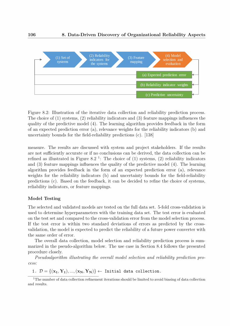
106 8. Data-Driven Discovery of Organizational Reliability Aspects
(1) Set of systems
(2) Reliability indicators for the systems
(3) Feature mapping
(4) Model selection and
evaluation
(b) Reliability indicator weights
(a) Expected prediction error
(c) Predictive uncertainty
Figure 8.2: Illustration of the iterative data collection and reliability prediction process.The choice of (1) systems, (2) reliability indicators and (3) feature mappings influences thequality of the predictive model (4). The learning algorithm provides feedback in the formof an expected prediction error (a), relevance weights for the reliability indicators (b) anduncertainty bounds for the field-reliability predictions (c). [138]
measure. The results are discussed with system and project stakeholders. If the resultsare not sufficiently accurate or if no conclusions can be derived, the data collection can berefined as illustrated in Figure 8.2 1: The choice of (1) systems, (2) reliability indicatorsand (3) feature mappings influences the quality of the predictive model (4). The learningalgorithm provides feedback in the form of an expected prediction error (a), relevanceweights for the reliability indicators (b) and uncertainty bounds for the field-reliabilitypredictions (c). Based on the feedback, it can be decided to refine the choice of systems,reliability indicators, or feature mappings.
Model Testing
The selected and validated models are tested on the full data set. 5-fold cross-validation isused to determine hyperparameters with the training data set. The test error is evaluatedon the test set and compared to the cross-validation error from the model selection process.If the test error is within two standard deviations of errors as predicted by the cross-validation, the model is expected to predict the reliability of a future power converter withthe same order of error.
The overall data collection, model selection and reliability prediction process is sum-marized in the pseudo-algorithm below. The use case in Section 8.4 follows the presentedprocedure closely.
Pseudoalgorithm illustrating the overall model selection and reliability prediction pro-cess:
1. D = {(x1,Y1), ..., (xN,YN)} ← Initial data collection.1The number of data collection refinement iterations should be limited to avoid biasing of data collection
and results.

8.3 Methodology - Statistical System Life Cycle Models 107
2. Sort D by system age.
3. Split D in Dtrain and Dtest with atest < as ≤ atrain.
4. Model Selection and Validation:
(a) Shuffle Dtrain randomly.
(b) Evaluate ErrCV by (nested) CV.
(c) Evaluate parameter weights w and predictive uncertainty for one fold.
(d) If Model has large ErrCV or predictive uncertainty then
• Change set of systems, reliability indicators, or feature mappingbased on expert discussions and jump to 4.
5. Model Testing:
(a) Train predictive model with Dtrain.
(b) Evaluate Errtest and compare with ErrCV .
(c) Evaluate parameter weights w and predictive distributions.
Algorithms
A vast range of algorithms for supervised regression problems exists. The requirementsin terms of uncertainty-quantification, reliability indicator relevance, and sparsity narrowdown the selection. A summary of the algorithms and their characteristics with respectto the requirements is presented in Table 8.1. The shown selection of algorithms is basedon their popularity for different problem domains, their simplicity, and their expectedsuitability for stochastic problems. The characteristics are listed in the columns and areuncertainty quantification (UQ), provision of a relevance measure, producing sparse mod-els, and global or local models. ARD and BAR algorithms fulfill all criteria.
Table 8.1: Summary of learning algorithms. Adapted from [138].
UQ Relevance Measure Sparsity Global/LocalARD yes yes yes GlobalBAR yes yes yes GlobalGP yes no no LocalENCV no yes yes GlobalSVR no only for linear kernel no Local
By formulating the reliability prediction problem as a supervised ML problem, we canchoose from a range of existing learning algorithms to generate the desired statistical modelfor predictive purposes. Since the uncertainty in the field-reliability predictions shall be

108 8. Data-Driven Discovery of Organizational Reliability Aspects
quantified (i.e. finding a model as presented in equation 8.5), the choice of algorithms isnarrowed down. Furthermore, sparse models are preferred since they potentially requirefewer reliability indicators to be collected and - more importantly - since they allow anestimation of the relevance of the choice of reliability indicators and the generated features.
Table 8.1 summarizes the chosen algorithms. The implementation from sklearn havebeen used [154]. Detailed descriptions of the methods can be found in their user guide[106]. A summary of each algorithm is given below:
• ARD - Automatic Relevance Determination Regression: A sparse Bayesian regressionmethod as introduced in [155] - Chapter 7.2.1. The implementation is described in[106] - Chapter 1.1.10.2.
• BAR - Bayesian Ridge Regression: A Bayesian regression method [156]. It resemblesARD Regression except for a simpler and less flexible parametrization of uncertaintywhich leads to fewer parameters that have to be learned from the data. It is describedin [106] - Chapter 1.1.10.1.
• GP - Gaussian Process Regression. A Bayesian Regression technique using the kerneltrick [157]. Its implementation is outlined in [158] - Algorithm 2.1 and was adaptedfrom [106] - Chapter 1.7.1. A combination of a radial-basis-function kernel and awhite-kernel is used. The kernel parameters are optimized during training.
• EN: Elastic Net Regression. A simple regression technique with regularization as de-scribed in [106] - Chapter 1.1.5. Hyperparameters are determined in a cross-validatedgrid-search.
• SVR - Support Vector Machine Regression: A regression method using the kerneltrick as described in [106] - Chapter 1.4.2. Linear basis functions are chosen and across-validated grid-search is used to determine the hyperparameters.
8.4 Numerical ExperimentsIn this section, the proposed approach is tested for a real use case. The goal is to find amodel to predict the reliability of magnet power converters used at CERN and to identifyrelevant factors influencing their reliability. The section is composed of an assessment ofdata requirements and actual data availability and quality, a set of model learning tasks,their results, and a discussion.
8.4.1 Data Requirements and AvailabilityData Requirements
The data collection requirements are outlined in the Data Collection subsection of Sec-tion 8.3. Most of its requirements are optional but leading to a better performance of the

8.4 Numerical Experiments 109
Table 8.2: Illustration of characteristic power converter attributes of the studied dataset.[138]
Power [W] Current [A] Voltage [U] Age [yrs] MTBF [hrs]Minimum 10−6 10−4 10−3 2.2 103
Maximum 108 4 · 104 105 49.7 6 · 105
method and easier interpretation of its results. Compulsory requirements are that relia-bility indicators and metrics are available for a set of systems, obtained in a coherent andidentical way, and based on sufficient operational experience so that they have stabilized.
In the following the collected data for the considered use case is described and whetherit fulfills the stated requirements is discussed. These are the chosen set of system types,reliability indicators, and reliability metrics.
Set of Systems More than 6000 power converters of around 600 different types are usedat CERN. A centralized computerized maintenance management system helps to tracktheir field reliability. Of the 600 converter types, 300 have a cumulative operation time ofmore than ten years and consistent data recordings. The remaining 300 are removed. Anoverview of minimal and maximal attributes of the 300 different selected converter typesare shown in Table 8.2 in terms of rated power, current, voltage, age and MTBF. It showsthat the data set contains a wide range of different power converters.
Reliability Indicators The selection of reliability indicators is based on recommen-dations of CERN engineers and project managers in charge of systems for complete lifecycles:2
1. Rated current of the converter (I). It influences the choice of technology for powerconversion. Current causes heating in systems which can be handled by appropriatethermal management [8, 6].
2. Rated voltage of the converter (U). Arcing or corona discharge can be caused by highvoltage. It requires the appropriate electrical insulation [8, 6].
3. Rated power of the converter (P). Power is the product of current and voltage. Hence,both above considerations can be valid for high powers.
4. Quantity of each power converter per converter type used at CERN (Quantity).When converters are produced in higher quantities, they tend to be handled differ-ently during life cycle phases. It may impact the reliability even though it is notrelated to any physical failure mechanism.
2The terms in brackets correspond to the acronym later used in figures to express the relevance of eachreliability indicator.

110 8. Data-Driven Discovery of Organizational Reliability Aspects
5. The average age of converters per type (Avg. Age). The age often has a stronginfluence on the reliability of systems due to wear-out mechanisms.
6. The cumulative age of converters per type (Cum. Age). Similar to the average agein term of wear-out mechanisms. However, the availability might also increase withcumulative age of systems as the organization learns to mitigate system deficiencies.
7. The polarity of the converter which indicates the operating modes, technology andcomplexity of the converter (Pol 0-9).3
8. The particle accelerator in which the converter is used (Acc. 1-9). Different accelera-tors have different operational environments in terms of radiation levels, operationalschedules, and maintenance strategies.
9. The count of different particle accelerators in which each converter is used (in Acc.).
Reliability Metrics The availability of the systems are expressed in terms of theirMTBF and MTTR which are calculated from the data of the Computerised MaintenanceManagement System (CMMS). To ensure validity of the data the raw fault and repairlogs were checked for converter types with conspicuous data. Moreover, converters withincomplete data or too little operational experience were removed.
The full data set D contains 281 different converter types with nine reliability indicators(see above) and two reliability metrics each, their MTBF and MTTR.
Data Availability and Quality Assessment
The data fulfills the above stated minimal requirements: reliability indicators and metricsare available for the set of systems, are obtained in a coherent and identical way, and arebased on sufficient operational experience.
The data was selected based on discussions with experts. However, not all recommendedindicators could be obtained for the several thousand converters. For example, operationaltemperatures might be relevant, but could not be collected. Nevertheless, the collectedindicators capture the main differences between the converter types. The majority ofindicators is available at early life cycle phases. Hence, any predictive model based onthese indicators can be used to predict the field reliability of a new converter early in itssystem life cycle.
8.4.2 Model Selection and ValidationThe full data set is split into a training set Dtrain, containing 210 converter types olderthan fifteen years, and a test set Dtest, containing 71 types of less than fifteen years. Hence,
3The discrete set of polarities is given by: (1) Unipolar, (2) Bipolar Switch Mechanic, (3) Bipolar I -Unipolar U - 2 Quadrants, (4) Unipolar I Bipolar U 2 Quadrants, (5) Bipolar Pulse-Width-Modulation, (6)Bipolar Relay, (7) Bipolar Electronic I/U, (8) Bipolar Anti-Parallel 4 Quadrants, (9) Bipolar I-circulation4 Quadrants and, (0) un-specified or other Polarity.[138]

8.4 Numerical Experiments 111
the test setting assumes that the prediction was carried out fifteen years ago based on theoperational experience up to that point in time.
As part of the model selection and validation process, the input data of the trainingfolds was normalized to a mean of zero and unit variance, as some of the selected learningalgorithms function better with scaled input data. The resulting scaling operator is laterapplied to the test folds. The logarithm of the reliability metrics, log(Y), is taken as outputdata for numerical purposes.
The following different configurations in terms of set of converter types, reliabilityindicators, and reliability indicator mappings are compared:
• Choice of converter types: The complete set of power converter types and a randomsub-selection of only 42 converter types is compared. The goal is to assess whether theuncertainty of predictions and reliability indicator relevance increases for a smallerdata set.
• Choice of reliability indicators: Models trained with the full set of reliability indica-tors are compared to those trained on a set without the quantity of converters pertype. The goal is to see whether removing an important indicator can be compen-sated and whether it can lead to different explanations of relevant factors for fieldreliability.
• Choice of reliability indicator mappings: Following features are generated based onthe reliability indicators:
– Linear features and logarithmic features are generated from numeric indicatorsxnum (indicators 1-6 and 9) - Φ(xnum) = [xnum, log(xnum)]T (resulting in 7+7values).
– Categorical indicators, for the polarity of the converters and the particle accel-erators in which the converter is used, xcat (indicators 7 and 8) are encoded intobinary features (resulting in 10+9 values).
– An additional constant set to 1.
This resulted in an input vector containing 34 values. Two mappings of this vectorwere chosen as input data:
– First order mapping: The input vector without additional transformation (ex-cept for the scaling operation).
– Second order mapping: A second order feature mapping to account for nonlinearinteractions between the reliability indicators,
Φ(xnum) =[xnum, log(xnum), [xnum, log(xnum)] · [xnum, log(xnum)]T
]T.
This results in 629 values for the input. The goal is to test whether a moreaccurate model can be generated when interactions between indicators are al-ready modeled at the level of the input data and whether the relevant factorsinfluencing the field reliability can still be retrieved.

112 8. Data-Driven Discovery of Organizational Reliability Aspects
The results of the model selection and validation are reported for each of the mentionedconfiguration in the following. The cross-validation mean squared error ErrCV and itsvariance on the hold-out sets is presented in tabular form and the predictions (MTBF andMTTR) and the reliability indicator relevance ρ are plotted for the last cross-validationfold. Only the predictions of the BAR algorithm are plotted to reduce the number ofoverall plots. BAR performs well across prediction tasks, produces sparse models, andquantifies uncertainty of predictions and indicator relevance. The predictive performanceof the algorithms can be assessed from the results Tables.
Reference Configuration The first configuration studied uses the complete set of con-verter types, all reliability indicators and the first order mapping. Applying the frameworkto the data set with the introduced model selection and validation scheme yielded the val-idation Meas-Squared-Error (MSE) shown in Table 8.3a for the MTBF and in Table 8.4afor the MTTR. It is observed that all algorithms (shown in different columns of the table)yield similar errors.
The obtained reliability predictions and their 95% highest probability density intervalon the hold-out set of the last validation fold4 of the BAR algorithm are shown in Fig-ure 8.3a for the MTBF and Figure 8.3c for the MTTR. The converter types (denotedSystem on the x-axis) are ordered by increasing predictedMTBF orMTTF , respectively.The orange line depicts the mean of the predictive distribution and the orange shaded areathe 95% confidence intervals. The blue dots mark the actual observed field-reliabilites. Itis observed that for the MTBF the variation could be captured accurately. However, theMTTR model does not manage to identify any relevant variations.
The obtained reliability indicator relevance (feature weight) of the last cross-validationfold is displayed in Figure 8.3b for the MTBF model and in Figure 8.3d for the MTTRmodel. The x-axis displays the different feature as obtained by the first order mappingof the collected reliability indicators. It is observed that similar indicators are relevantacross different algorithms. The logarithm of the quantity of converters produced per typelog(Qty) is the dominant factor.
It is very interesting to note that the logarithm of the quantity of converters per typeis the most relevant factor in achieving an accurate reliability prediction. Obviously, thequantity is only a correlating and not a causal factor. Nevertheless, this hints at non-technical factors being relevant for the reliability of magnet power converters in this usecase. A closer investigation might reveal causal factors, which are overlooked in technicalanalysis.
The fact that all models yield similar errors and assign similar relevance to similarfactors is giving confidence in the results. It also suggests that due to the randomness ofthe prediction task, sophisticated algorithms do not lead to better results. Hence, it wasnot studied to use deep learning methods to improve the predictions.
As theMTTR models did not identify any dependencies they are not discussed further.4The size of the hold-out set correspond to one fifth of the training set of 210 converters. This is 42,
which is by chance the same amount as the reduced set of training systems but should not be confused.

8.4 Numerical Experiments 113
0 10 20 30 40System
6
7
8
9
10
11
12
13
ln(M
TBF)
(a)
Qua
ntity
Cum
. Age
Avg.
Age
I U PPo
l 0Po
l 1Po
l 2Po
l 3Po
l 4Po
l 5Po
l 6Po
l 7Po
l 8Po
l 9co
nsta
ntAc
c. 1
Acc.
2Ac
c 3.
Acc.
4Ac
c. 5
Acc.
6Ac
c. 7
Acc.
8Ac
c. 9
Acc.
10
in A
cc.
log(
Qty
.)lo
g(C
u. A
.)lo
g(Av
. A.)
log(
I)lo
g(U
)lo
g(P)
0.5
0.0
0.5
1.0
1.5Fe
atur
e W
eigh
t ENSVRARDBAR
(b)
0 10 20 30 40System
0
2
4
6
8
10
ln(M
TTR
)
(c)
Qua
ntity
Cum
. Age
Avg.
Age
I U PPo
l 0Po
l 1Po
l 2Po
l 3Po
l 4Po
l 5Po
l 6Po
l 7Po
l 8Po
l 9co
nsta
ntAc
c. 1
Acc.
2Ac
c 3.
Acc.
4Ac
c. 5
Acc.
6Ac
c. 7
Acc.
8Ac
c. 9
Acc.
10
in A
cc.
log(
Qty
.)lo
g(C
u. A
.)lo
g(Av
. A.)
log(
I)lo
g(U
)lo
g(P)
0.4
0.2
0.0
0.2
0.4
Feat
ure
Wei
ght
ENSVRARDBAR
(d)
Figure 8.3: Results for the reference configuration. (a),(c): Prediction of the log(MTBF )and log(MTTR) by the BAR algorithm for the last fold of the cross-validation procedure.The orange line depicts the mean of the predictive distribution and the orange shaded areathe 95% confidence intervals. The blue dots mark the actual observed field-reliabilites.Note that the converter types on the x axis of the last cross-validation fold were orderedby the mean of the predictions to recognize whether trends are properly captured. (b),(d):Estimated feature weights for the parametric models. [138]

114 8. Data-Driven Discovery of Organizational Reliability Aspects
Reduced Set of Training Systems In the second configuration of only 42 randomlysub-selected converter types, it is tested whether a reduction of the data set affects theidentified models and their predictive and parametric certainty. The obtained validationMSEs ErrCV in Table 8.3b for the MTBF and Table 8.4b for the MTTR are larger thanthe values obtained with the reference data set. Nevertheless, the reliability indicatorrelevances (Figure 8.4b for MTBF and Figure 8.4d for MTTR) are identified similarly tothe reference configuration. Variations in the MTBF are captured accurately again (seeFigure 8.4a). Variations in the MTTR are not properly captured (see Figure 8.4c), as wasthe case for the reference configuration.
The biggest difference appears in the certainty of the predictions (orange shaded area inFigures 8.4a and 8.4c) and relevance measures (uncertainty bars in Figures 8.4b and 8.4d),which are much larger than in the reference configuration. This confirms the expectedbehavior, as the algorithms have to learn from much fewer data.
Reduced Set of Reliability Indicators In the third configuration, it is tested whetheromitting relevant reliability indicators can be compensated and whether it suggests conflict-ing conclusions in terms of relevant factors influencing reliability. To do so, the logarithmof the quantity of converters per type log(Qty) is removed.
The resulting MSEs for the MTBF (Table 8.3c) are almost three times those of thereference configuration, whereas the MSEs of the MTTR (Table 8.4c) increased slightly.The MTBF reliability indicator relevance (Figure 8.5b) do not identify a single dominantfactor anymore; the most relevant being the logarithm of the rated power log(P ) with anegative influence on the reliability. It did also have a negative influence for the referenceconfiguration. The MTTR reliability indicator relevance (Figure 8.5d) are comparable tothe ones identified for the reference configuration. For the predictions (Figure 8.4a for theMTBF and Figure 8.4c for the MTTR ) it is observed that in neither for the MTBF norfor the MTTR the variations are properly captured and that the uncertainties increaseboth for predictions and relevance estimates.
It is concluded that in this case the omission of a relevant indicator cannot be compen-sated. Furthermore, the relevant factors influencing reliability do not suggest conflictingconclusions in this scenario. However, a wider study is suggested to confirm these findingsgenerally.
Second-Order Feature Mapping The fourth configuration tests whether the second-order feature mapping allows for more accurate modeling of reliability. The resultingMSEs ErrCV (Table 8.3d for the MTBF and Table 8.4d for the MTTR) are comparableto those obtained with the reference configuration except for the model generated by ARDalgorithm which performs significantly worse.
The second-order mapping yielded 629 features, which are not illustrated as their visualinterpretation is not possible. The predictions are illustrated in Figure 8.5e for theMTBFand in Figure 8.5f for theMTTR. They perform similarly to the predictions obtained withthe first order mapping of the reference configuration.
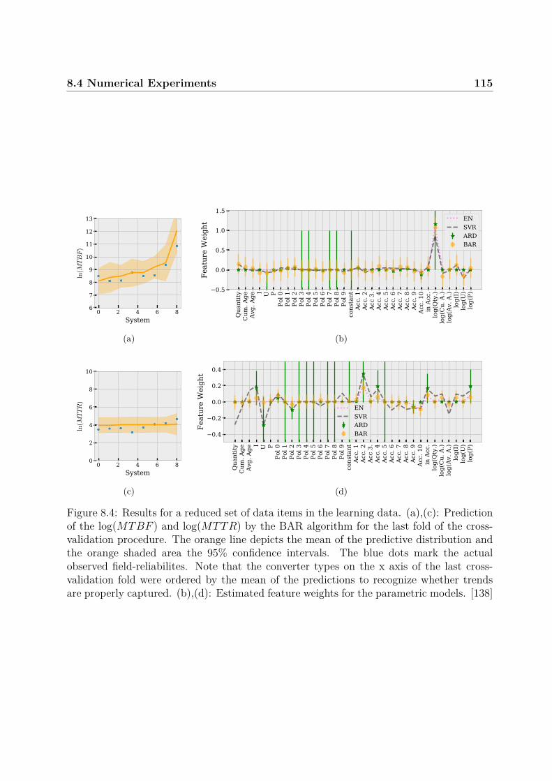
8.4 Numerical Experiments 115
0 2 4 6 8System
6
7
8
9
10
11
12
13
ln(M
TBF)
(a)
Qua
ntity
Cum
. Age
Avg.
Age
I U PPo
l 0Po
l 1Po
l 2Po
l 3Po
l 4Po
l 5Po
l 6Po
l 7Po
l 8Po
l 9co
nsta
ntAc
c. 1
Acc.
2Ac
c 3.
Acc.
4Ac
c. 5
Acc.
6Ac
c. 7
Acc.
8Ac
c. 9
Acc.
10
in A
cc.
log(
Qty
.)lo
g(C
u. A
.)lo
g(Av
. A.)
log(
I)lo
g(U
)lo
g(P)
0.5
0.0
0.5
1.0
1.5Fe
atur
e W
eigh
t ENSVRARDBAR
(b)
0 2 4 6 8System
0
2
4
6
8
10
ln(M
TTR
)
(c)
Qua
ntity
Cum
. Age
Avg.
Age
I U PPo
l 0Po
l 1Po
l 2Po
l 3Po
l 4Po
l 5Po
l 6Po
l 7Po
l 8Po
l 9co
nsta
ntAc
c. 1
Acc.
2Ac
c 3.
Acc.
4Ac
c. 5
Acc.
6Ac
c. 7
Acc.
8Ac
c. 9
Acc.
10
in A
cc.
log(
Qty
.)lo
g(C
u. A
.)lo
g(Av
. A.)
log(
I)lo
g(U
)lo
g(P)
0.4
0.2
0.0
0.2
0.4
Feat
ure
Wei
ght
ENSVRARDBAR
(d)
Figure 8.4: Results for a reduced set of data items in the learning data. (a),(c): Predictionof the log(MTBF ) and log(MTTR) by the BAR algorithm for the last fold of the cross-validation procedure. The orange line depicts the mean of the predictive distribution andthe orange shaded area the 95% confidence intervals. The blue dots mark the actualobserved field-reliabilites. Note that the converter types on the x axis of the last cross-validation fold were ordered by the mean of the predictions to recognize whether trendsare properly captured. (b),(d): Estimated feature weights for the parametric models. [138]

116 8. Data-Driven Discovery of Organizational Reliability Aspects
Table 8.3: Obtained mean-squared-errors for the log(MTBF ) - a) ErrCV for the referencemodel, b) ErrCV for a reduced set of systems, c) ErrCV for a reduced set of reliabilityindicators, d) ErrCV for nonlinear numeric feature mappings, and e) Errtest for the predic-tions of the test data-set. Comparison of a) and e) indicates if the method can be extendedto future converter types. [138]
ARD BAR GP EN SVRErrCV a) 0.39±0.15 0.35±0.13 0.37±0.14 0.34±0.12 0.46±0.16ErrCV b) 0.90±0.79 0.82±0.73 0.81±0.74 0.65±0.49 0.64±0.50ErrCV c) 1.03±0.24 1.00±0.19 1.00±0.19 1.01±0.22 1.02±0.24ErrCV d) 0.59±0.23 0.37±0.05 0.38±0.05 0.32±0.05 0.48±0.12Errtest e) 0.30 0.33 0.32 0.30 0.38
It is concluded that the predictive performance is not improved by the second orderfeature mapping. This is expected, as it is similar to using more complex modeling ap-proaches, which also do not lead to better predictions. Besides that, interpreting the 629features can pose a problem.
8.4.3 PredictionThe reference configuration is identified as the most suitable modeling approach in themodel selection and validation procedure. It is used to perform the reliability predictionand relevant factor identification on the whole data set. Models are learned using dataof converters more than 15 years old and tested on data of converters of less than 15years, as previously described. Hence, if the reliability of the more recent converters isaccurately predicted based on older ones, it provides strong evidence that the reliability offuture converters can be predicted accurately based on current ones. Only the MTBF ispredicted as no predictive MTTR model could be identified during model selection.
The obtained test MSEs Errtest are shown in Table 8.3e. They are slightly better thanthe predicted generalization errors ErrCV , but also lie within their standard deviation,as estimated in the cross-validation procedure during model selection. This gives furtherconfidence in the results. The reliability indicator relevance (Figure 8.6b) and the reliabilitypredictions (Figure 8.6a) on the test set are consistent with the model validation resultsas well. Overall, it is demonstrated that the MTBF can be predicted and most relevantfactors identified accurately.
8.4.4 DiscussionFor this use case, several points can be noted. Firstly, with the collected data it is possibleto predict the reliability of future converters with an accuracy that is on par with existingmethods [139]. However, the effort for data collection and modeling is greatly reduced and

8.4 Numerical Experiments 117
0 10 20 30 40System
6
7
8
9
10
11
12
13
ln(M
TBF)
(a)
Cum
. Age
Avg.
Age
I U PPo
l 0Po
l 1Po
l 2Po
l 3Po
l 4Po
l 5Po
l 6Po
l 7Po
l 8Po
l 9co
nsta
ntAc
c. 1
Acc.
2Ac
c 3.
Acc.
4Ac
c. 5
Acc.
6Ac
c. 7
Acc.
8Ac
c. 9
Acc.
10
in A
cc.
log(
Cu.
A.)
log(
Av. A
.)lo
g(I)
log(
U)
log(
P)
0.4
0.2
0.0
0.2
0.4
Feat
ure
Wei
ght
ENSVRARDBAR
(b)
0 10 20 30 40System
0
2
4
6
8
10
ln(M
TTR
)
(c)
Cum
. Age
Avg.
Age
I U PPo
l 0Po
l 1Po
l 2Po
l 3Po
l 4Po
l 5Po
l 6Po
l 7Po
l 8Po
l 9co
nsta
ntAc
c. 1
Acc.
2Ac
c 3.
Acc.
4Ac
c. 5
Acc.
6Ac
c. 7
Acc.
8Ac
c. 9
Acc.
10
in A
cc.
log(
Cu.
A.)
log(
Av. A
.)lo
g(I)
log(
U)
log(
P)
0.4
0.2
0.0
0.2
0.4
Feat
ure
Wei
ght
ENSVRARDBAR
(d)
0 10 20 30 40System
6
7
8
9
10
11
12
13
ln(M
TBF)
(e)
0 10 20 30 40System
0
2
4
6
8
10
ln(M
TTR
)
(f)
Figure 8.5: (a),(c),(e),(f): Prediction of the log(MTBF ) and log(MTTR) by the BARalgorithm for the last fold of the cross-validation procedure. The orange line depictsthe mean of the predictive distribution and the orange shaded area the 95% confidenceintervals. The blue dots mark the actual observed field-reliabilites. Note that the convertertypes on the x axis of the last cross-validation fold were ordered by the mean of thepredictions to recognize whether trends are properly captured. (b),(d): Estimated featureweights for the parametric models. Figures (a),(b),(c),(d) are for the configuration with areduced set of reliability indicators and Figures (e),(f) for the second-order feature mapping.Note that the illustrations of the 629 second-order feature weights are omitted. [138]

118 8. Data-Driven Discovery of Organizational Reliability Aspects
0 20 40 60System
7
8
9
10
11
12
13
ln(M
TBF)
(a)
Qua
ntity
Cum
. Age
Avg.
Age
I U PPo
l 0Po
l 1Po
l 2Po
l 3Po
l 4Po
l 5Po
l 6Po
l 7Po
l 8Po
l 9co
nsta
ntAc
c. 1
Acc.
2Ac
c 3.
Acc.
4Ac
c. 5
Acc.
6Ac
c. 7
Acc.
8Ac
c. 9
Acc.
10
in A
cc.
log(
Qty
.)lo
g(C
u. A
.)lo
g(Av
. A.)
log(
I)lo
g(U
)lo
g(P)
0.5
0.0
0.5
1.0
1.5
Feat
ure
Wei
ght EN
SVRARDBAR
(b)
Figure 8.6: (a): Predictions of the log(MTBF ) with the final models for the test data-set. The orange line depicts the mean and the orange shaded area the 95% confidenceintervals. The blue dots mark the actual observed field-reliabilites. Note that the differentconverter types were ordered by the mean of the predictive distribution. (b):Estimatedfeature weights for the predictive models. [138]
Table 8.4: Obtained mean-squared-errors for the log(MTTR) - a) ErrCV for the referencemodel, b) ErrCV for a reduced set of systems, c) ErrCV for a reduced set of reliability indi-cators, d) ErrCV for nonlinear numeric feature mappings, and e) Errtest for the predictionsof the test data-set. [138]
ARD BAR GP EN SVRErrCV a) 0.23±0.05 0.22±0.0.04 0.22±0.04 0.22±0.04 0.23±0.05ErrCV b) 0.32±0.17 0.24±0.11 0.24±0.12 0.23±0.09 0.25±0.17ErrCV c) 0.30±0.16 0.23±0.06 0.23±0.06 .28±0.11 0.29±0.16ErrCV d) 3.12±4.83 0.23±0.02 0.23±0.03 0.22±0.02 0.34±0.06Errtest e) 0.38 0.35 0.35 0.35 0.36

8.5 Chapter Summary, Conclusions and Outlook 119
independent of the complexity of the studied system, which can be critical for complex sys-tems. The uncertainty of the overall process can be systematically captured, and relevantfactors affecting the field reliability can be revealed.
Secondly, the most relevant indicator for an accurate prediction is the quantity ofproduced converters per type. This indicator is available very early during a system lifecycle. Hence, a reliability prediction based on such an indicator is available at the beginningof the life cycle of a new converter when it is most valuable. It can be used as input tomodel the availability of a whole accelerator complex.
Thirdly, using complex modeling strategies with better modeling flexibility do not leadto better prediction results. Most likely, this is due to the stochasticity of the problem.The choice of the right reliability indicators has the strongest impact on the predictiveperformance of the learned models.
8.5 Chapter Summary, Conclusions and OutlookAn approach to predict the reliability of systems is presented. It allows to quantify therelevance of factors influencing reliability as well as the uncertainty of the overall modelingprocess. For a power converter use case it is demonstrated that theMTBF can be predictedwith state of the art performance at a reduced data collection and modeling effort.
The quantity of produced converters per type was the factor with the highest relevancefor predicting reliability. Hence, the prediction can be carried out at the beginning of asystem life cycle, as this indicator is already available then. The output of this study canbe used as input for particle accelerator reliability optimization studies. The reduced datacollection and modeling effort in comparison to traditional reliability prediction methodswill make accurate reliability estimates available for more systems and hence improve themodeling of the overall particle accelerator reliability.
For future work, the causal factors behind the correlation of the produced quantityof converters per type with field reliability should be closer investigated. It hints at therelevance of factors not covered by traditional reliability analysis, which focuses on tech-nical aspects. Moreover, the overall methodology should be validated for a wider range ofsystems.
Chapter Learning Summary
The findings indicate that reliability is influenced by all processes during a systemlife cycle. Instead of focusing on isolated aspects, such as the system design, allprocesses should be evaluated for their impact on reliability.

120 8. Data-Driven Discovery of Organizational Reliability Aspects

Chapter 9
Synthesis: Developing RobustData-Driven Reliability OptimizationMethods
In the previous three chapters, data-driven reliability optimization methods for differentscenarios have been presented. They provide solutions to a wide range of representativechallenges in industrial applications. This chapter combines the findings of the previouschapters to answer the Umbrella RQ. It is structured as follows:
• Section 9.1 is a critical assessment of the previous three constructive chapters to ver-ify that the tailored CRISP-DM methodology helps to resolve practical limitationsof data-driven reliability optimization methods. It consists of two parts: Firstly,Subsection 9.1.1 evaluates whether the practical limitations have been addressedsuccessfully in each of the constructive methods of Chapters 6-8. Secondly, Subsec-tion 9.1.2 studies the usefulness and potential improvements of the tailored CRISP-DM methodology.The critical assessment confirms that practical limitations are resolved and thatthe CRISP-DM methodology is useful. The assessment also reveals that two ad-ditional aspects, which are necessary to use the reliability optimization methodscost-effectively, are not covered in the previous chapters. These are the correct tim-ing when applying reliability optimization methods within a system life cycle and theprovision of high-quality data for the methods. These two aspects and their solutionsare discussed in the two following sections.
• Section 9.2 discusses the optimal timing of each constructive method within a systemlife cycle to maximize their effectiveness.
• Section 9.3 lists the types of data required for reliability optimization methods. Sug-gestions are made for the effective collection and provision of these data in highquality.

1229. Synthesis: Developing Robust Data-Driven Reliability Optimization
Methods
• Finally, Section 9.4 combines all the previous findings and provides a cost-effectivedata-driven reliability optimization framework for complex engineered systems, whichaddresses the Umbrella RQ.
9.1 Critical Assessment of Constructive Chapters
9.1.1 Addressing Practical LimitationsThe aim of this section is to assess whether the limitations of existing works, as introducedin Section 4.2, have been addressed appropriately by the methods developed in Chapters 6-8. All existing limitations are listed in Tables 9.1 and 9.2, respectively, and assessed foreach of the developed methods. Each line in the table corresponds to an existing limitation.It is described in the first column and assessed for each of the methods from Chapters 6-8in the columns marked Ch5-7. Additional remarks are given in the comment column.
The tables shows all stated limitations have been either fully or partially addressed bythe presented data-driven reliability optimization methods. Nevertheless, some trade-offsremain, which are discussed in the following:
• The lack of fault data: This trade-off arises from fundamental conflicts of interest.As soon as a system has one or several faults, investigations will be started. It willnot be waited until the system has accumulated a sufficient number of failures sothat quantitative estimates can be made with high confidence. Hence, such methodswill always be used at the limits of statistical validity.To alleviate associated risks, methods in this thesis provide explanations of theirpredictions and an uncertainty-quantification. Thereby, a human expert can assesswhether a model learned from few data is technically sound or not.An alternative approach would be to use methods that only use the healthy systemstate as reference and detect deviations from it. Usually, there is sufficient data tocharacterize the healthy state of a system. However, such approaches cannot detectwhether a deviation of system leads to a failure or not. Hence, replacing or stopping asystem with a deviating behavior can prove highly uneconomical because it might notlead to failure. In complex systems, such as particle accelerators, where operationalsettings are frequently changed, deviating behavior is often expected not to lead tofailure. Therefore, such methods have not been further investigated in this thesis.
• Life cycle phases without monitoring: Although tracing and monitoring of productsduring shipping or storage can be implemented (e.g. [159]), it is questionable whethercomplete monitoring and information exchange throughout all life cycle phases isfeasible and cost-effective. Hence, in practice such solutions are rare for reliabilitypurposes.In the fourth line of Table 9.1 it is written that the problem of un-monitored lifecycle phases is ’Implicitly addressed’ by the developed methods of Chapter 6-8. This

9.1 Critical Assessment of Constructive Chapters 123Ta
ble9.1:
Evalua
tionof
prop
osed
solutio
nsagainstlim
itatio
nsof
relatedwo
rk-p
art1.
Lim
ita
tio
ns
of
rela
ted
wo
rks.
C
h5
Ch
6
Ch
7
Co
mm
ent
Sco
re
Exis
ting
stu
die
s ar
e m
ost
ly c
arri
ed o
ut
on a
co
mp
on
ent
lev
el,
oft
en c
on
sider
ing
on
ly s
ingle
fai
lure
mod
es. H
ow
ever
, in
rea
lity
syst
ems
are
com
pose
d o
f m
any
co
mp
on
ents
and
are
aff
ecte
d b
y
mu
ltip
le, oft
en o
ver
lap
pin
g f
ailu
re m
od
es a
nd
mec
han
ism
s.
Add
ress
ed
Add
ress
ed
Add
ress
ed
All
Met
hod
s h
ave
bee
n
app
lied
to
rea
list
ic
scen
ario
s
4
Man
y s
tudie
s do
no
t ac
coun
t fo
r th
e d
epen
den
ce o
f fa
ilu
re
mec
han
ism
s o
n m
ult
iple
fac
tors
. A
dd
ress
ed
Can
be
incl
uded
wit
h E
yri
ng
mod
el
Impli
citl
y
add
ress
ed
Use
d m
ult
ivar
iate
dat
a-
dri
ven
ap
pro
ach
3
Dyn
amic
env
iron
men
ts a
nd
un
fore
seen
in
pu
ts c
an o
ften
not
be
robust
ly h
and
led
by
dat
a d
riv
en m
ethod
s.
Add
ress
ed
(but
not
test
ed
syst
emat
ical
ly)
Add
ress
ed
Impli
citl
y
add
ress
ed
Dat
a dri
ven
met
ho
ds
can
be
pro
ble
mat
ic. H
andle
d
by
Ap
pro
pri
ate
mod
el
sele
ctio
n s
chem
es
3
Deg
rad
atio
n d
oes
not
only
hap
pen
duri
ng
oper
atio
n o
f sy
stem
s.
Sy
stem
s ar
e ex
pose
d t
o s
tres
ses
du
ring
tra
nsp
ort
, st
ora
ge
and
inst
alla
tion
, w
hic
h c
an r
emai
n u
nobse
rved
by
mon
ito
ring
sy
stem
s.
Impli
citl
y
add
ress
ed
Can
be
incl
uded
A
dd
ress
ed
Dat
a ac
quis
itio
n
chal
leng
ing
. 2
-3
Of
all
64
pap
ers…
only
in
7 p
aper
s it
was
att
empte
d t
o v
alid
ate
the
dev
elop
ed m
ethod
olo
gie
s w
ith
fie
ld d
ata
incl
udin
g a
ny
des
crip
tion
of
the
dat
a co
llec
tion
.
Add
ress
ed
Add
ress
ed
Add
ress
ed
Inte
gra
l p
art
of
con
stru
ctiv
e m
ethod
olo
gy
4
An
un
cert
ainty
qu
anti
fica
tion
and
pro
pag
atio
n t
hro
ugh
out
all
step
s
in r
elia
bil
ity
mod
elin
g i
s es
sen
tial
. N
ot
addre
ssed
A
dd
ress
ed
Add
ress
ed
Tra
nsp
aren
cy o
f m
eth
ods
allo
ws
ad h
oc
cert
ain
ty
asse
ssm
ent.
3
Met
hods
pro
pose
d i
n t
he
lite
ratu
re i
mp
lici
tly
req
uir
e a
wel
l
funct
ionin
g m
onit
ori
ng
of
equip
men
t, c
om
pu
ting
in
fras
tru
ctu
res,
and
exis
ting
dat
a se
ts o
f ru
n t
o f
ailu
re d
ata.
How
ever
, m
any
org
anis
atio
ns
can
not
mee
t th
ese
requ
irem
ents
. T
he
met
hods
dev
elop
ed i
n t
his
th
esis
do
not
requ
ire
add
itio
nal
har
dw
are
inv
estm
ents
, bu
t m
ake
use
of
sensi
ng
in
form
atio
n w
hen
ever
read
ily
av
aila
ble
.
Add
ress
ed
Add
ress
ed
Add
ress
ed
In s
om
e ca
ses
exce
llen
t
mon
itori
ng
in
fras
tru
ctu
re
avai
lable
4
Sik
ors
ka
et a
l [1
37
] an
d A
n e
t al
[8]
crit
icis
e th
at e
xis
ting
rev
iew
pap
ers
focu
s on
mat
hem
atic
al a
spec
ts o
f d
iffe
ren
t m
eth
ods
inst
ead
of
the
val
ue
of
the
met
hod
s in
rel
iabil
ity
opti
miz
atio
n c
onte
xts
.
Add
ress
ed
Add
ress
ed
Add
ress
ed
Inte
gra
l p
art
of
con
stru
ctiv
e m
ethod
olo
gy
. 4

1249. Synthesis: Developing Robust Data-Driven Reliability Optimization
MethodsTa
ble9.2:
Evalua
tionof
prop
osed
solutio
nsagainstlim
itatio
nsof
relatedwo
rk-p
art2.
Lim
ita
tio
n
Ch
5
Ch
6
Ch
7
Co
mm
ent
Sco
re
Ther
e is
a l
ack
of
stan
dar
diz
ed a
ppro
ach
es w
hic
h w
ou
ld h
elp
pra
ctit
ion
ers
nav
igat
e th
e v
ast
cho
ice
of
opti
ons.
Par
tial
ly
add
ress
ed
Par
tial
ly
add
ress
ed
Par
tial
ly
add
ress
ed
Met
hod
co
mp
aris
on
an
d
sele
ctio
n t
hro
ug
h
lite
ratu
re r
evie
w.
3
Tid
den
s et
al
[13
9]
sho
wed
that
pra
ctit
ion
ers
choo
se t
he
met
hods
for
reli
abil
ity
op
tim
izat
ion
bas
ed o
n t
he
exp
erie
nce
of
pro
ject
sta
keh
old
ers
or
oth
er c
om
pan
ies
and
av
aila
bil
ity
of
read
y-t
o-u
se i
mple
men
tati
ons
inst
ead
of
syst
emat
ical
ly c
ho
osi
ng
an a
pp
rop
riat
e ap
pro
ach
fro
m t
he
beg
innin
g.
Add
ress
ed
Add
ress
ed
Add
ress
ed
Met
hods
chose
n b
ased
on
lit
erat
ure
rev
iew
.
Pro
ject
s o
nly
car
ried
out
afte
r fe
asib
ilit
y a
sses
sed
.
4
Anoth
er f
req
uen
tly
en
coun
tere
d c
hal
len
ge
is t
he
pro
vis
ion
of
dat
a w
hic
h c
an m
eet
the
req
uir
emen
ts o
f th
e d
evel
op
ed m
etho
ds
and
su
bse
quen
tly
supp
ort
eff
ecti
ve
dec
isio
n m
akin
g.
Su
ffic
ient
dat
a S
uff
icie
nt
Dat
a
Su
ffic
ient
Dat
a
Dat
a av
aila
bil
ity
and
qual
ity
ass
esse
d. O
ther
pro
ject
s w
ith
insu
ffic
ient
dat
a re
ject
ed.
4
They
pro
po
se a
un
iver
sal
met
ric
to m
easu
re d
ata
fitn
ess
for
pu
rpo
se a
nd
org
anis
atio
nal
ince
nti
ves
to
im
pro
ve
dat
a q
ual
ity
.
Add
ress
ed
qual
itat
ivel
y
Add
ress
ed
qual
itat
ivel
y
Add
ress
ed
qual
itat
ivel
y
Dat
a av
aila
bil
ity
and
qual
ity
ad
dre
ssed
qual
itat
ivel
y. N
o m
etri
c
use
d.
4
Oth
er p
roble
ms
in d
ata
coll
ecti
on
are
the
lack
of
stan
dar
diz
ed
way
s fo
r dat
a co
llec
tio
n a
nd
th
e la
ck o
f k
no
wle
dg
e of
fail
ure
mod
es w
hic
h s
ho
uld
def
ine
the
rele
van
t dat
a to
co
llec
t.
Sem
i
stan
dar
diz
ed.
Fai
lure
mod
es
know
n. F
ailu
re
mec
han
ism
s
unkn
ow
n.
Sta
nd
ardiz
ed.
Fai
lure
mec
han
ism
s
know
n.
Sta
nd
ardiz
ed.
Fai
lure
mod
es n
ot
app
lica
ble
.
Sta
nd
ardiz
ed d
ata
coll
ecti
on
not
alw
ays
obse
rved
to
lea
d t
o
impro
vem
ents
.
3
An
et
al [
8]
enco
ura
ges
th
e sh
arin
g o
f d
ata
sets
as
the
exis
tin
g
ben
chm
ark
dat
a se
ts a
re l
imit
ed i
n t
hei
r use
fuln
ess.
Dat
a par
tial
ly
on
git
hub
. C
an
be
req
ues
ted
fro
m t
he
auth
or.
Can
be
requ
este
d
fro
m t
he
auth
or.
Can
be
requ
este
d
fro
m t
he
auth
or.
3
As
poin
ted
out
by
Sun
et
al [
138
] p
rogn
ost
ics
can
pro
vid
e m
any
add
itio
nal
ben
efit
s ac
ross
th
e sy
stem
lif
e cy
cle.
Esp
ecia
lly
wh
en
it c
an b
e use
d t
o i
mp
rove
the
nex
t gen
erat
ion
of
syst
ems
at e
arly
life
cy
cle
stag
es, th
e ex
pec
ted
cost
ben
efit
is
larg
est.
Yie
ldin
g a
few
insi
gh
ts u
sefu
l
acro
ss l
ife
cycl
es.
Yie
ldin
g
som
e
insi
gh
ts
use
ful
acro
ss
life
cy
cles
.
Yie
ldin
g
insi
gh
ts
use
ful
acro
ss
life
cy
cles
.
Sy
stem
atic
way
to
der
ive
insi
ghts
acr
oss
life
cy
cles
pre
sente
d
late
r in
th
is c
hap
ter.
3

9.1 Critical Assessment of Constructive Chapters 125
does not mean that they collect data from all life cycle phases, but that they canappropriately handle situations with missing life cycle data. The method from Chap-ter 6 would adapt its reliability model when the monitored system is affected fromprevious un-monitored damage. The models from Chapter 7 and Chapter 8 can in-clude monitoring and damage data if they are available. However, if such data is notavailable, the additional uncertainty due to lack of data will be quantified.
• Complexity of methods: The complexity of realistic scenarios often demands theuse of complex methods. Such methods require advanced mathematical skills fromproject stakeholders for the correct use of the methods and the interpretation of theirresults. For the core teams involved in the presented use cases, this could be ensured.However, for a wider adoption of the methods and effective use, special training wouldbe necessary. It is noticed that with the emergence of ML as a discipline of its ownand the associated education becoming more prevalent, the adoption of complexdata-driven methods is facilitated.
Besides these trade-offs, two other aspects are critical for cost-effective reliability im-provement, which have not been addressed in the constructive chapters:
• The optimal embedding of the presented methods in a system life cycle for cost-effective reliability optimization.
• The effective collection and provision of the data required for reliability optimization.
These two aspects and their solutions are presented in detail in Section 9.2 and Sec-tion 9.3, respectively. Before these two aspects are covered, the usefulness of the tailoredCRISP-DM methodology is assessed in the following subsection.
9.1.2 Usefulness of the Tailored CRISP-DM MethodologyHaving confirmed that practical limitations can be overcome in the previous section, thegoal of this section is to assess whether the tailored CRISP-DM methodology for methoddevelopment is appropriate.
This is examined by evaluating the usefulness of the recommended steps as stated inthe methodology description (Section 5.2) for each of the use cases from Chapters 6-8.Tables 9.3 and 9.4 list the stated recommendations, the degree to which they have beenadopted in each of the constructive chapters, and additional comments on the usefulnessof each recommendation.
To summarize the tables, the CRISP-DM methodology with its minor adaptations hasbeen very appropriate for the considered reliability optimization projects. The step of amodeling method evaluation in addition to establishing the decision objectives and assess-ing the data availability has proven useful to determine the correct modeling approaches.Moreover, the strict separation between project assessment and project implementationhas been helpful to avoid investment of time and effort into projects, which are deemed tobe unsuccessful.

1269. Synthesis: Developing Robust Data-Driven Reliability Optimization
MethodsTa
ble9.3:
Evalua
tionof
prop
osed
CRISP-
DM
metho
dology
-part1.
Met
ho
do
log
y S
tep
(R
eco
mm
end
ati
on
) R
Q1
RQ
2
RQ
3
Co
mm
ent
Th
e fi
rst
step
is
to i
den
tify
th
e ob
ject
ive
and
th
e m
ean
s [o
f th
e
reli
abil
ity o
pti
miz
atio
n p
rob
lem
].
Per
form
ed
Per
form
ed
Per
form
ed
Ver
y u
sefu
l bu
t o
ften
ov
erlo
ok
ed.
Ob
ject
ive
oft
en i
mp
reci
sely
def
ined
by p
roje
ct r
equ
esto
rs.
Th
e ob
ject
ive
sho
uld
be
conv
erte
d i
nto
a m
easu
rab
le q
uan
tity
,
such
as
cost
, re
liab
ilit
y o
r a
com
bin
atio
n t
her
eof.
Par
tial
ly
Per
form
ed
Par
tial
ly
Per
form
ed
Par
tial
ly
Per
form
ed
Qu
alit
y o
f p
redic
tio
ns
qu
anti
tati
vel
y
mea
sura
ble
wh
en o
bje
ctiv
e is
cle
ar.
Qu
alit
y o
f ex
pla
nat
ion
s d
iffi
cult
to
mea
sure
. N
eed
s in
vo
lvem
ent
of
use
rs o
f dev
elo
ped
met
hod
s.
To
furt
her
nar
row
dow
n t
he
choic
e o
f [p
ote
nti
al m
eth
od
s] a
lite
ratu
re r
evie
w i
s ca
rrie
d o
ut.
P
erfo
rmed
P
erfo
rmed
P
erfo
rmed
Tim
e-co
nsu
min
g p
roce
ss. F
ew
revie
w p
aper
s fo
cus
on
use
fuln
ess
of
met
hod
s in
the
conte
xt
of
pro
ject
ob
ject
ives
an
d d
om
ain
.
Fo
r ea
ch [
pote
nti
al m
ethod
s] t
he
min
imu
m a
nd
op
tim
al d
ata
and
kn
ow
led
ge
requir
emen
ts a
re a
sses
sed
. T
hen
the
actu
al d
ata
and
kn
ow
led
ge
avai
lab
ilit
y i
s co
mp
ared
agai
nst
its
requ
irem
ents
.
Per
form
ed
Per
form
ed
Per
form
ed
Ver
y i
mp
ort
ant
step
to
ass
ess
pro
ject
fea
sibil
ity a
t ea
rly s
tage.
Dat
a val
idit
y a
nd
consi
sten
cy n
eed
s
to b
e ch
eck
ed a
s w
ell.
Th
e co
mp
atib
ilit
y o
f o
bje
ctiv
es, m
eth
od
s, a
vai
lable
dat
a an
d
kno
wle
dg
e ar
e co
nfi
rmed
. S
uff
icie
nt
soft
war
e, h
ard
war
e an
d
tim
e re
sou
rces
fo
r im
ple
men
ting
th
e m
od
elin
g s
trat
egie
s n
eed
to b
e av
aila
ble
.
Per
form
ed.
Per
form
ed
Per
form
ed
Sli
gh
tly r
edund
ant
if p
rev
iou
s st
eps
carr
ied o
ut
app
rop
riat
ely.
Har
dw
are
and
so
ftw
are
req
uir
emen
ts c
ou
ld
dev
elop
wit
h p
roje
ct p
rog
ress
.
Th
e m
issi
ng
dat
a an
d k
now
ledg
e is
co
llec
ted
by r
unnin
g
exp
erim
ents
, in
terv
iew
ing
syst
em e
xp
erts
, an
d l
iter
atu
re
rese
arch
. R
eadil
y a
vai
lable
dat
a is
cle
aned
, val
idat
ed w
ith
syst
em e
xp
erts
to
en
sure
dat
a qu
alit
y m
eets
its
req
uir
emen
ts,
and
sto
red
in
an
acc
essi
ble
fo
rmat
.
Per
form
ed
Per
form
ed
Per
form
ed
Dat
a val
idat
ion
of
imp
ort
ance
.
Req
uir
es i
nte
ract
ion
wit
h s
yst
em
exp
erts
. T
ime
con
sum
ing
.
No
add
itio
nal
exp
erim
ents
fo
r d
ata
gen
erat
ion
nee
ded
in
use
cas
es.
It i
s ben
efic
ial
to e
mp
loy s
ever
al m
etho
ds
in p
aral
lel
and
com
par
e th
eir
ou
tputs
. P
erfo
rmed
P
erfo
rmed
P
erfo
rmed
Giv
es c
on
fid
ence
in
fin
din
gs
wh
en
dif
fere
nt
met
ho
ds
yie
ld s
ame
resu
lts.
Par
t o
f m
od
el s
elec
tion
pro
cedu
re
for
mac
hin
e le
arnin
g.

9.1 Critical Assessment of Constructive Chapters 127Ta
ble9.4:
Evalua
tionof
prop
osed
CRISP-
DM
metho
dology
-part2.
Met
ho
do
log
y S
tep
(R
eco
mm
end
ati
on
) R
Q1
RQ
2
RQ
3
Co
mm
ent
Wh
enev
er a
nov
el m
ethod
is
imp
lem
ente
d,
it i
s fi
rst
test
ed o
n a
kn
ow
n p
rob
lem
to
ver
ify a
ll f
unct
ion
alit
ies
are
wo
rkin
g a
s ex
pec
ted
. W
hen
th
e n
ov
el m
eth
od
pas
ses
this
test
su
cces
sfu
lly, it
is
app
lied
to
th
e ac
tual
pro
ble
m.
Per
form
ed
Per
form
ed
Par
tial
ly
Per
form
ed
No
t st
rict
ly n
eces
sary
wh
en u
sing
triv
ial
and
tes
ted
met
hods.
If
kn
ow
n
pro
ble
m d
oes
not
exis
t, s
yn
thet
ic
dat
a ca
n b
e u
sed
.
Su
cces
sful
imp
lem
enta
tio
n o
f th
e o
pti
miz
atio
n m
etho
d a
llo
ws
to d
eter
min
e th
e dec
isio
n p
aram
eter
s w
hic
h l
ead
to
the
bes
t
outc
om
e. P
roje
ct s
takeh
old
ers
are
info
rmed
abou
t th
e
reco
mm
end
ed d
ecis
ion
s an
d i
ts j
ust
ific
atio
n.
Par
tial
ly
Per
form
ed
Per
form
ed
Par
tial
ly
Per
form
ed
En
d-t
o-e
nd
un
cert
ain
ty
quan
tifi
cati
on
ver
y u
sefu
l to
giv
e
dec
isio
n c
on
fid
ence
. In
dat
a d
riv
en
met
hods,
th
e ju
stif
icat
ion
has
to
be
ver
ifie
d w
ith
syst
em e
xp
erts
.
To
val
idat
e th
at t
he
sugg
este
d d
ecis
ions
are
actu
ally
lea
din
g t
o
the
des
ired
ou
tco
me
in t
he
lon
g t
erm
req
uir
es f
oll
ow
-up
aft
er
imp
lem
enta
tion
.
Par
tial
ly
Per
form
ed
Par
tial
ly
Per
form
ed
Par
tial
ly
Per
form
ed
Sim
ula
tion
bas
ed v
alid
atio
n f
or
use
case
s. L
on
g t
erm
cost
and
rel
iab
ilit
y
foll
ow
up
chal
lengin
g.
Imp
lem
enta
tio
ns
can
oft
en b
e re
use
d f
or
rela
ted
pro
ject
s du
e to
the
mo
du
lar
stru
ctu
re o
f d
ata
dri
ven
fra
mew
ork
s.
Per
form
ed
Per
form
ed
Per
form
ed
Mod
ula
r st
ruct
ure
of
pro
ject
s
faci
lita
tes
reuse
. O
ften
su
ffic
ient
to
adap
t d
ata
load
ing
in
terf
ace.
[CR
ISP
-DM
met
hodo
log
y]
step
s ca
n b
e re
pea
ted
, th
e ord
er
does
not
hav
e to
be
foll
ow
ed s
tric
tly, an
d t
he
imp
lem
enta
tio
ns
can
be
upd
ated
con
tinu
ousl
y.
Per
form
ed
Per
form
ed
Per
form
ed
Ste
ps
wer
e o
ften
rep
eate
d, bu
t o
rder
not
mix
ed.
Imp
ort
ant
to c
arry
ou
t
feas
ibil
ity a
sses
smen
t bef
ore
an
y
imp
lem
enta
tion
ste
ps.
To
avo
id u
np
lann
ed p
roje
ct f
ailu
res,
utm
ost
im
po
rtan
ce i
s p
aid
to i
nit
ial
ph
ases
of
the
CR
ISP
-DM
met
hodo
log
y o
f B
usi
nes
s
and
Dat
a U
nd
erst
andin
g. M
ore
ov
er, an
addit
ion
al p
has
e o
f
Mod
el U
nd
erst
andin
g i
s ad
ded
in
pro
ject
s of
this
thes
is.
Per
form
ed
Per
form
ed
Per
form
ed
Ver
y u
sefu
l. O
ther
pro
ject
s (n
ot
repo
rted
) w
ith
out
pri
or
feas
ibil
ity
asse
ssm
ent
had
to
be
can
cell
ed a
t
late
r pro
ject
sta
ges
. S
yst
emat
ic
asse
ssm
ent
wo
uld
hav
e pre
ven
ted
pro
ject
inv
estm
ents
.

1289. Synthesis: Developing Robust Data-Driven Reliability Optimization
Methods
Two minor improvements can be suggested: Firstly, the requirements definition forexplanations provided by the implemented methods should receive more attention duringthe objectives definition stage. However, assigning appropriate goals and metrics for qual-itative explanation outputs are more difficult than for quantitative predictive outputs ingeneral and especially at such early project stages.
Secondly, the proposed long-term validation of any implemented method is difficultto realize. It would require follow-up over years and it is uncertain whether the effectsfrom a certain method can be disentangled from effects due to other methods. To reducethe associated risks, the methodology recommends to test the methods extensively onbenchmark problems or in simulation before they are used for decision support.
9.2 Embedding Data-Driven Reliability OptimizationMethods in System Life Cycles
In this section, the goal is to embed the reliability optimization methods from Chapters 6-8within a system life cycle so that they can be used effectively. As illustrated in Figure 1.1,reliability optimization methods are generally more cost-effective when they support deci-sion making in early life cycle phases.
The phases of a system life cycle, the main engineering tasks at each phase, and popularestablished reliability methods and their role within different life cycle phases are presentedat the end of Section 3.1. On this basis, the optimal integration of the optimization methodsis discussed as described below.
In the following three subsections, each of the methods from Chapters 6-8 are charac-terized by their required (data) inputs and when they are available during a life cycle, aswell as their outputs and how they can be used to improve system reliability. A distinc-tion is made between systems with and without predecessors for which reliability expertisehas already been accumulated, as this makes a difference for the usage of the methods.Differences to established reliability methods and how they can be complemented by themethods introduced in Chapters 6-8 are discussed.
In the fourth and final subsection, it is described how the methods can be used tosupport decision making in early life cycle phases, which leads to cost-effective reliabilityoptimization.
9.2.1 Embedding Data-Driven Discovery of Failure MechanismsThe method from Chapter 6, which addresses RQ1, can be used to predict and identifyfailure mechanisms in systems from their logging and monitoring data. The required inputknowledge is limited to a selection of logging or monitoring signals, which signify thefailures that one aims to predict, as well as a range of signals, which are expected tocontain precursors of the relevant failures. The outputs of the method are predictions offaults in advance and a selection of the most relevant precursors of these faults, from whichthe failure mechanism can be inferred by experts.
9.2 Embedding Data-Driven Reliability Optimization Methods in System LifeCycles 129
This method has the advantage that it requires almost no a-priori system knowledge.However, it requires monitoring data of the studied system. Hence, for a system withoutpredecessors, it can mainly be used as soon as a data logging environment has been setup. This may happen after prototyping or production. The choice of monitoring signalsto consider can be guided by the results of an FMEA analysis. The output of the methodcan be used in an online and offline setting. In an online use, arising operational issuesare predicted and mitigated by experts before they happen. In an offline use, failuremechanisms are detected and mitigation measures discussed. Again, the results of anFMEA analysis can guide the identification of failure mechanisms. The outputs may triggerfurther reliability investigations that use the inferred knowledge on failure mechanisms asinput.
For systems with predecessors, the usage of the method is similar. The previouslyaccumulated knowledge allows a more focused selection of relevant precursor and failuremonitoring signals. However, more abstract knowledge, such as pre-existing failure behav-ior quantification, cannot be utilized by the method.
The classical equivalent of the data-driven method would be manual monitoring andfailure analysis by machine operators and experts. Manual analysis is effective when (1) fewor only a single failure have been observed, (2) the operators and experts are experiencedand knowledgeable with the affected systems, and (3) the set of potential root-causes ofthe fault is small (e.g. because the affected systems are simple). Contrary to that, theintroduced method is effective when (1) several faults have been observed, (2) the operatorsand experts are neither experienced nor knowledgeable about the affected systems, and (3)the set of potential root causes is large (because the affected systems are complex andinterconnected).
In summary, the method is best suited for complex systems with sufficient monitoringdata and limited expert knowledge. Its output helps to avoid arising operational failuresand to build up expert knowledge on failure mechanisms within a complex system.
9.2.2 Embedding Data and Knowledge-Driven Parametric Model-Based Reliability Optimization
The method from Chapter 7, addressing RQ2, utilizes expert knowledge, failure data, andscientific literature to develop quantitative models of failure behavior. With a simulationengine, optimal operation and maintenance strategies are derived. The required inputsinclude quantification of failure behavior as a function of the operational conditions, aswell as knowledge on the intended future system usage and costs associated with repairsand downtime events. The output is an expected system life cycle cost, which serves asdecision metric for different operational, maintenance, and design strategies.
The advantage of this method is that it can effectively combine all available sourcesof knowledge. The required quantification of failure behavior can be obtained from op-erational experience from predecessor systems, established models and parameters fromscientific literature, or reliability testing. For systems without predecessors, reliability
1309. Synthesis: Developing Robust Data-Driven Reliability Optimization
Methods
testing can be carried out as soon as prototypes are available. To refine prediction modelsand to account for differences between the prototypes and the final systems, the reliabilitytests should be repeated after the production stage. Moreover, models should be con-tinuously updated during operational phases. Bayesian parameter estimation techniquesprovide a systematic way for updating model parameters. Thereby, the quality of predic-tions of the models increase continuously and can be used to optimize operations of theexisting system, as well as successor systems.
Successors, which reuse parts of the design, can also reuse the corresponding parts ofthe reliability models. Changed or newly introduced parts of the system have to be treatedas systems without predecessors.
The introduced method is an extension of established reliability techniques. Theseinclude (accelerated) reliability testing, acceleration factor models, Weibull analysis, MonteCarlo simulation, and life cycle cost modeling. Whereas the established methods are used atcertain life cycle stages only, the introduced method allows to combine data and knowledgeacross life cycle stages and reuse it for future derivations of systems. Overall, the methodis best suited to combine various sources of data and knowledge across a system life cycleand use it to optimize the operation of existing and future systems.
9.2.3 Embedding Data-Driven Discovery of Organizational Reli-ability Aspects
The method from Chapter 8, addressing RQ3, predicts the expected field reliability offuture systems as well as the most relevant factors influencing it based on the experiencewith existing comparable systems. The required input is a measured field reliability forthe existing systems and a range of quantitative reliability indicators selected by expertsfor both the existing systems as well as the systems for which the reliability should bepredicted. The method provides reliability predictions for new systems and the factorswith a positive or negative impact on reliability.
The stage at which the method can be used to predict the reliability of a system dependson the set of relevant reliability indicators that have been identified. In the presented usecase, the relevant indicators are already available at the concept stage of a life cycle. Hence,the reliability of a future system can be predicted at its concept stage already.
Comparable established reliability prediction methods have been outlined in Section 8.2.They are mostly characterized by focusing on technical aspects and certain life cycle phases.Hence, they can only be used when sufficient technical information about the system isavailable. Moreover, their modeling and data collection effort is coupled to the complexityof the studied system. In contrast, the introduced method integrates non-technical aspectsseamlessly and considers all system life cycle phases. The effort for modeling and datacollection is independent of the complexity of the investigated systems. Hence, it is recom-mended to use the introduced method when (1) non-technical aspects shall be considered,(2) the systems are complex, or (3) when predictions need to be available very early in thelife cycle of a system.

9.3 Improving Data Quality through Automatic Reliability Data Collection131
9.2.4 Using the Methods for Cost-Effective Decision MakingTo use the presented methods as tools for cost-effective reliability optimization, they needto be integrated in system life cycles in a way that they can support engineering decisionmaking at early stages of the life cycle. This subsection assesses how to achieve this foreach of the methods addressing RQ1-3, respectively.
The method addressing RQ3 satisfies above-mentioned requirement by providing reli-ability predictions and relevant factors at early life cycle stages. The methods addressingRQ1 and RQ2 do not satisfy this requirement up-front. Both provide useful outputs onlyafter a system has been built and operated for some time.
However, the results of the RQ2 method can be reused for optimising future similarsystems at early life cycle stages. Moreover, the RQ1 method can provide outputs that fa-cilitate the implementation of the RQ2 method by indicating the relevant failure precursorsand mechanisms. Hence, an iterative approach emerges: It starts with data-driven meth-ods to explore fault patterns and mechanisms and inform system experts (RQ1 method).Then, it continues with model-driven methods (RQ2 method), which allow system expertsto combine their built-up knowledge with the fault data to generate transparent quantifi-cation of failure behavior, which can be reused for future systems optimization.
This combination of data and model-driven methods across life-cycle allows to improvethe reliability of future systems cost-effectively in early life cycle stages. Finally, theRQ3 method can help assessing the effectiveness of the employed reliability optimizationmethods in the long term.
9.3 Improving Data Quality through Automatic Re-liability Data Collection
Throughout the use cases, provision of sufficient and high-quality reliability data was anissue. However, such data is crucial for a cost-effective implementation of the presentedmethods. This section presents potential solutions to address data provision issues basedon evidence from the literature and experience from use cases in this thesis.
The scarcity of reliability data has been reported and studied in literature (see Sec-tion 4.2). The reasons for insufficient data are both of technical and organizational kind.
Technical reasons include that failures can be complex emergent phenomena that arehard to monitor and understand. Sensing and monitoring is expensive, increases the com-plexity of a system, and can introduce new failure modes.
Organizational reasons include that the responsibility of data taking is not assigned,teams responsible for data taking are not given enough context or incentives to carry itout properly, data needs to be stored and maintained over many years, and lastly that theprocess from data taking to effective decision for reliability optimization is complex andinvolves many steps and people.
To provide potential solutions to data provision issues, this section• lists the types of data required for reliability optimization,

1329. Synthesis: Developing Robust Data-Driven Reliability Optimization
Methods
• provides recommendations for designing a system to automatically collect the re-quired data, and
• provides recommendations for organising a project to facilitate manual collection therequired data.
9.3.1 Types of Data Required for Reliability OptimizationFor each of the reliability optimization scenarios in this thesis, a list of minimal datarequirements and recommendations for optimal data provisioning has been compiled inthe constructive chapters. Comparing the compiled data requirements reveals a significantoverlap, although the scenarios cover a wide range of different reliability optimizationscenarios, objectives, and methods. Hence, it is concluded that across many reliabilityoptimization tasks, similar kind of data is required, which facilitates the provision of datacollection guidelines.
The required data types for the reliability optimization scenarios of this thesis arelisted below. These data are grouped by the requirements of different characteristic re-liability modeling approaches. These are lifetime models (Weibull models, accelerationfactor models, statistical reliability models), system condition models (Physics-of-Failuremodels, data-driven remaining useful life models), or qualitative evaluation models (Paretoanalysis, design reviews; not presented in the thesis but dealt with during preparation ofuse cases):
1. System identifiers: system ID, assembly ID, component ID
2. Failure identifiers: fault timestamp, fault location (e.g. connector xyz), fault effect(e.g. open circuit), fault mechanism (e.g. corrosion), root cause (e.g. humiditybecause water leak)
3. Data for lifetime models:
• System utilization time until failure• Suspension times: times/dates switched off, (Optional:) times in other usage
before current use, (Optional:) times in storage and shipping before usage• Sample size: Number and ID of components, assemblies, or systems of the same
type• (Optional:) Downtime due to failure• (Optional:) Downtime unrelated to failure• (Optional:) Operating condition history (mostly relevant if non-uniform across
sample)
4. Data for system condition models:
• Operational loads
9.3 Improving Data Quality through Automatic Reliability Data Collection133
• Environmental loads• System condition indicators
5. Data for qualitative assessment methods:
• Design documentation• Manufacturing documentation• Repair documentation
The first two items are required for all reliability investigations. The necessity of the thirdand fourth item depend on the type of modeling and decision objective. The fifth item isusually required to provide data on fault mechanisms and root causes.
The data types for system condition models (item 4) are only vaguely defined in thelist. Methods to determine the precise kind of required data for system condition modelscan be found in the literature [147, 160, 44, 24, 45]. A few general guidelines are given inthe following: The output of an FMEA analysis helps to identify failure precursors thatare likely to occur and deserve monitoring. Indicators, which are cheap to measure andlikely to cover several failure modes, should be prioritized as they are expected to improvethe cost-effectiveness of monitoring. An example for electronic systems is the differencebetween input and output power, which indicates the dissipated power. An increase ofpower dissipation can be an indicator for a range of failure modes.
Having the listed data types available in high quality is expected to facilitate theachievement of a large variety of common reliability optimization objectives. Recommen-dations for the effective collection of these data items are provided in the following twosubsections. The recommendations are not conclusive but should serve as starting pointsfor future investigations.
9.3.2 Design for Automatic Reliability CollectionDesigning automatic data collection mechanism into systems would be a promising ap-proach for cost-effective provision of data. However, not all data collection procedures canbe automated.
Criteria to assess whether automatic collection and storage of data through sensors,networks, and databases are feasible and economic are (0) the necessity and utility ofthe data for reliability optimization, (1) the feasibility of automatising, (2) band-widthrequirements, and (3) storage requirements for data logging. In the following, the datatypes listed in the previous subsection are grouped by the expected automation capabilityof their collection according to the criteria above and data collection considerations arediscussed for each group.
• System identifiers, the fault timestamp, the sample size, and most data for systemcondition models are well suited for automated collection and storage. The imple-mentation of an automatic collection system is not expected to be challenging.

1349. Synthesis: Developing Robust Data-Driven Reliability Optimization
Methods
• A range of data items might qualify for automatic collection. These are the faultlocation and effect, system utilization time until failure, times and dates a systemhas been switched off, times in storage and shipping, and downtime (un-/)related tofailures.All these data, except for times in storage and shipping, are related to a fault or anunavailability of a system. Hence, the fault or unavailability can affect the monitoringsystem, which is supposed to collect the considered data automatically. Therefore, itis necessary to design automatic collection systems in a fault proof way so that a faultneither in the monitored system nor in the monitoring system causes inconsistenciesin the data collection. Although such fault tolerant fault monitoring systems exist[161, 162], their cost-effectiveness has to be assessed for each scenario.The times in storage and shipping can principally be collected automatically withadditional monitoring efforts. However, when a system is stored, handled and shippedproperly, the aging and reliability effects should be limited [8] and monitoring is notjustifiable.
• The remaining data items can partially be collected automatically. This includes thefault mechanism and root cause.The fault mechanism and root cause can be automatically detected for recurring andexpected faults for which diagnostic systems are "designed-in". For new emergentfault behavior, it is unlikely that a reliable automatic mechanism and root causediagnosis system, which works without additional expert input, can be developed.A human expert analysis, assisted by semi-automatized diagnostic systems, such asintroduced in Chapter 6, is expected to be more cost- and time-effective for identi-fying novel fault mechanisms and root-causes. In the following subsection, organiza-tional factors, which encourage system stakeholders to carry out such manual failureanalysis and reporting in detail, are discussed.
9.3.3 Organization for Automatic Reliability Data CollectionSome data or information is most effectively collected by human experts. Especially failuremechanisms and root causes of novel and complex failures require manual analysis andvalidation by system experts. These analysis need to generate high-quality data to beuseful for reliability optimization methods.
Based on the literature from Section 4.2 and experience from use cases in this thesis,the following factors improve the quality of manually collected reliability data:
• Data collectors need to be aware of the value of data collection for an organization.They need to understand the potential use of the data that they collect and havesufficient expertise on the systems they investigate.
• The responsibility for data collection has to be assigned. Appropriate means forreliability data collection have to be considered for a system at early life cycle stages.

9.4 A Data-Driven Framework for Cost-Effective Continuous ReliabilityOptimization 135
• Across use cases it is observed that the quality of collected data improves whenthe data collection responsibility is assigned to experts, which were involved in theconception and design of a system.
Further recommendations for improving organizational data collection practices are pro-vided by Unsworth et al [71].
9.4 A Data-Driven Framework for Cost-Effective Con-tinuous Reliability Optimization
In this section, a proposal for a data-driven reliability optimization framework based onthe previous findings is presented. Section 9.1 confirms that the developed reliability op-timization methods resolve many practical limitations, Section 9.2 presents an embeddingof these optimization methods within system life cycles to use them cost-effectively, andSection 9.3 outlines how sufficient data of high quality can be provided for the optimizationmethods.
The proposed framework combines the previous findings and leads to cost-effectivedata-driven system reliability optimization for complex engineered systems by overcomingmany practical limitations:
1. Automatic Reliability Data Collection: Systems and processes need to be designedwith data collection for reliability analysis and corresponding decision making inmind. A detailed listing of relevant data as well as guidelines for the implementationof effective data collection methods are presented in Section 9.3. These data shouldbe available to stakeholders throughout the system life cycle.
2. Automatic data-driven failure pattern identification: A data-driven approach to ob-tain predictive models of system failures and supporting information on failure mech-anisms from logging data as presented in Chapter 6. The predictive models can helpto prevent unforeseen failures and the failure mechanism information simplifies failureanalysis for complex systems.
3. Degradation quantification and generalization: A systematic approach to combinefailure mechanism information, failure data and expert knowledge into a transparentquantification of system degradation as presented in Chapter 7. It can be generalizedto systems with different operating conditions and reused for future generations ofsystems.
4. Reliability prediction and effectiveness evaluation: The recorded field reliability of asystem can be correlated with factors characterising its system life as presented inChapter 8. For a set of comparable systems, multivariate statistical models can beobtained. They allow to estimate future systems’ field reliability at early life cyclestages and provide insight on the factors that impact reliability, which enables earlystrategic decision making.

1369. Synthesis: Developing Robust Data-Driven Reliability Optimization
Methods
The framework can be integrated into system life cycles and complement existing reliabilityefforts.
Chapter Learning Summary
Reliability data collection should be designed into systems at early life cycle phases.Effective use of data mining methods reveals insights that improves future systems’reliability.

Chapter 10
Conclusions and Future ResearchDirections
The complexity of modern engineered systems keeps increasing. At the same time, demandson reliability are growing. Traditional techniques, which are based on manual expertanalysis, are reaching their limits in such situations and new approaches are required.
Modern data-science methods provide a possible solution. Such methods handle com-plex and dynamic data, which are common for modern systems but challenging for tra-ditional approaches. They can extract valuable information from the increasing volumesof data, which are accumulated during operation of modern technical infrastructures, tohelp operators and experts improving the reliability of their infrastructures. As an exam-ple for one of the most complex technical infrastructures, this thesis focuses on particleaccelerators, such as the LHC.
Despite the potential of modern data-science methods, they frequently fail in practicalreliability optimization scenarios because they make too simplistic assumptions of thesystem behavior, do not consider organizational contexts for cost-effectiveness, and buildon specific monitoring data, which are too expensive to record.
The goal of this thesis is to resolve these practical limitations and better leverage thecapabilities of modern data-science methods. This has been achieved by the followingcontributions:
• A methodology for the development and implementation of practical data-drivenreliability optimization methods, which address previous limitations and considersorganizational contexts. It is based on the CRISP-DM methodology consisting of aproject assessment and implementation phase.For three realistic use cases, it is demonstrated that applying the methodology ledto the development of data-driven reliability optimization methods for addressingexisting limitations and advance the state-of-the-art. The diversity of mathematicalmodeling approaches and reliability optimization objectives used across the scenariosis matched by few other studies in the field of reliability optimization. The contri-butions of the three methods to the state-of-the-art are detailed below.

138 10. Conclusions and Future Research Directions
1. Explainable deep learning methods predict failures in modern technical infras-tructures and help to explain their failure mechanisms. This helps to increasesystem availability directly by predicting impeding failures and their precursorsas well as indirectly by assisting experts to build up their expertise on how toimprove the system.The presented method is among the first experimental studies of ExplainableAI in time-series applications and demonstrates the advantages of deep learningtechniques over existing approaches based on Support Vector Machine, RandomForest, or kNearestNeighbor methods for modeling the complexity of realisticphenomena. The generality of the method allows its application to other do-mains where the discovery of mechanisms in time series data is crucial.
2. Hierarchical parametric models allow to combine expert knowledge and oper-ational data throughout the system life cycle for improved reliability modelaccuracy. Together with a Monte-Carlo simulation engine and an end-to-enduncertainty-quantification, the system operations and associated life cycle costcan be optimized. The transparent modeling structure allows generalizing re-sults to new operating conditions as well as reusing models and parameters tooptimize future generations of systems cost-effectively.The method is a realization of the digital twin concept and among the mostmatured examples in the reliability domain. As such, it serves as a valuablereference for the further development of digital twin solutions for reliabilitypurposes.
3. The field-reliability of systems and its most influencing factors can be predictedwith multivariate statistical models. They are trained on reliability data as wellas on quantified life cycle descriptors for a group of comparable systems. Incomparison to traditional reliability prediction methods, this allows to performmore accurate reliability predictions at earlier life cycle phases for a wider rangeof systems at reduced modeling efforts. Moreover, it can be used to disentanglethe effects of various reliability improvement methods on the field-reliability.
• For the success of all three methods, the collection and provision of high-quality datais crucial. Section 9.3 contributes a list of data types that are required for a rangeof common reliability optimization objectives as well as recommendations for theeffective collection of these data. These are derived with a systematic approach toidentify data requirements across optimization objectives and with a translation ofthe obtained requirements into concrete suggestions for improving the data collectionand provisioning.
• Finally, to increase the cost-effectiveness of the methods, their optimal embeddingwithin the different phases of the system life cycle is derived in Section 9.2 withrespect to the availability of data and the optimal timing of decision making. Thecost-effective embedding and combined use of reliability optimization methods acrosssystem life cycles has not been covered elsewhere.

10.1 Future Research Directions 139
The contributions of this thesis push data-driven reliability optimization methods asubstantial step closer to succeeding in realistic environments. It is demonstrated thatthese methods have the potential to improve the reliability of systems and reduce theircost at reduced additional capital and labor investment. For future generations of technicalinfrastructures, specifically particle accelerators, effective use of such methods might provecritical to ensure high reliability at reduced cost despite the continuously growing systemcomplexity.
10.1 Future Research DirectionsThe findings of this thesis suggest a range of potential future research directions. Theseare grouped in three blocks:
1. Future data-science techniques and their impact on the presented methods.
2. Future research on the usage and application of the presented methods.
3. Future research on applying the findings of this thesis to other domains.
With respect to 1., future data-science techniques are expected to have a positive impacton the cost-effectiveness, user friendliness, and the range of applications of the presentedmethods:
• Few-Shot Learning (FSL) could extend the use of data-driven methods to scenarioswith even less failure data to learn from.
• Bayesian parameter identification methods can combine data from prototype testsas well as operation in a systematic manner including quantification of uncertainty.User friendly, open source tools for such assessments are currently not available.
• Symbolic regression might provide more intuitive model interpretations than cur-rently used input relevance measures.
With respect to 2., future research on the usage of the presented methods could leadto improved guidelines for practitioners:
• Objective criteria should be identified to judge whether traditional knowledge-drivenor advanced data-driven reliability optimization methods are more suited for specificscenarios.
• The tailored CRISP-DM methodology should be validated and refined for reliabilityoptimization projects not covered by the three considered representative scenarios.
With respect to 3., future research on applying the findings of this thesis to otherdomains could help to advance other areas of applied data-science:

140 10. Conclusions and Future Research Directions
• The method from Chapter 6 can be applied to domains where the discovery andunderstanding of mechanisms in time series data is critical.
• The method from Chapter 7 serves as a valuable reference for the further developmentof digital twin solutions in industrial environments.
• The systematic approach to improve the collection and provision of high-quality datafrom Section 9.3 could prove useful for other applied data-science domains, which areaffected by insufficient data of low quality.
• The approach from Section 9.2 to embed data-driven optimization methods withina system life cycle to maximize cost-effectiveness can be generalized to other data-driven optimizations in organizational contexts.
Learning Summary
Using modern data-science methods delivers new approaches in many different fields.In this thesis, the practical applicability of such methods for reliability optimizationof complex technical infrastructures is demonstrated in general and for the particleaccelerators of CERN in particular.

List of Figures
1.1 Cost of change in an engineering project throughout a system life cycle. [6] 41.2 Evolution of computing devices over recent decades in terms of volume,
price, and number of installed devices. . . . . . . . . . . . . . . . . . . . . 5
2.1 Schematic overview of the CERN accelerator complex. [29] . . . . . . . . . 152.2 Simplified illustration of the four superimposed rings of the PSB and its
beam transfer lines. [32] . . . . . . . . . . . . . . . . . . . . . . . . . . . . 162.3 Layout of the PSB and its beam transfer lines. [33] . . . . . . . . . . . . . 172.4 Schematic overview of a power converter. . . . . . . . . . . . . . . . . . . . 19
3.1 Life cycle cost for different maintenance strategies for a hypothetical examplewith (a) low equipment cost and (b) high equipment cost. For low equipmentcost, fault tolerance is the most cost-effective solution. For high equipmentcost, condition-based maintenance is the most cost-effective solution. . . . 29
3.2 Raw collected data of tyre wear. . . . . . . . . . . . . . . . . . . . . . . . . 333.3 Linear fit to raw data. . . . . . . . . . . . . . . . . . . . . . . . . . . . . . 333.4 Linear fit after cleaning data. Fit to data before cleaning captured wrong
trend. . . . . . . . . . . . . . . . . . . . . . . . . . . . . . . . . . . . . . . 343.5 High order polynomial function achieves lower MSE than linear fit. However,
it does not capture the trend correctly: Overfitting . . . . . . . . . . . . . 353.6 Evaluation of linear fit on cleaned data on newly arrived test data. Appar-
ently, data collection for initial data was biased. . . . . . . . . . . . . . . . 363.7 Scatter plot of new extended multivariate data set, containing engine strength,
driver behavior, driven mileage, and tyre profile depth as variables. His-tograms of each variable the diagonal. Scatter plots of all combinations ofany two variables on off-diagonals. Clear dependence only visible for profiledepth as function of mileage driven. . . . . . . . . . . . . . . . . . . . . . . 37
3.8 Feature weights (θ1) of the linear multivariate model fitted to training data.Learning a model based on all features improves the predictive performanceof the model. Hence, all features are considered relevant. The mileage is themost important feature. . . . . . . . . . . . . . . . . . . . . . . . . . . . . 38
142 LIST OF FIGURES
3.9 Reformulation of problem as classification problem by defining a thresholdfor acceptable car tyre profile depth. A classifier aims to find a separationboundary between class ’acceptable’ (orange dots) and ’not acceptable’ (bluecrosses). . . . . . . . . . . . . . . . . . . . . . . . . . . . . . . . . . . . . . 39
5.1 (a) The original CRISP-DM methodology. [73] (b) Adapted CRISP-DMmodel. . . . . . . . . . . . . . . . . . . . . . . . . . . . . . . . . . . . . . . 49
6.1 Upper Row: ML algorithms are able to identify animal species based onlabeled images. Explanation techniques help to understand which pixelscontribute the most to assign a certain species to an input image. [93] LowerRow: Logged time series are accumulated during the operation of a particleaccelerator. A sliding window approach extracts a data set consisting ofinputs characterising the relative past behavior of the system and outputsindicating if a specific alarm or fault occurs in the relative future, whichis shown in the left cell (Data). This generates a supervised training dataset without manual labeling effort. Based on this data set, a model canbe learned to predict certain system alarms and faults, which is shown inthe middle cell (Data Driven Model Prediction). LRP can then be used tohighlight the most relevant input signals in the past that precede a fault inthe future, which is shown in the lower right cell (Explanation). It highlightsthat only two alarms (darker blue) are relevant for the fault. [75] . . . . . 59
6.2 Time discrete model formulation. The x-axis represents discrete time andthe y-axis monitoring signals of the investigated infrastructure. Crossesmark events that could be faults, alarms, changes in monitoring values, etc.Events of the signal SN represent infrastructure faults that the model Φ(·)predicts. [75] . . . . . . . . . . . . . . . . . . . . . . . . . . . . . . . . . . 61
6.3 Parameters of synthetic pattern. The Sp signal contains deterministic pre-cursors. Two following signals cause a fault signal SFs . A range of randomlyactivated noise signals, SR1 , SR2 , ..., represent non-relevant parts of the in-frastructure. [75] . . . . . . . . . . . . . . . . . . . . . . . . . . . . . . . . 69
6.4 Dependency of the predictive performance on the number of randomly firingsignals. The line depicts the mean and the error bar plus and minus onestandard deviation calculated over the 7 validation sets. Solid lines representdeep models, which perform on average better than the classical models(dashed). (a) The F1 score. Note that the predictors level out at 0.0 forlarge nrand, which is the binary F1 score when always predicting the majorityclass (’0’). (b) The accuracy. The predictors level out at 0.82 for large nrand,which is the accuracy when always predicting the majority class (’0’). [75] 70
6.5 Parameters of synthetic pattern. An infrastructure fault, SFb , happens whensimultaneous failures of the two interacting sub-systems, SP1 and SP2 , fulfilla Boolean AND, OR, or XOR condition. Four additional non-interactingsub-systems, SR1−4 , randomly trigger alarms that do not lead to a fault. [75] 70

LIST OF FIGURES 143
6.6 Illustration of AND, OR and XOR fault logic extraction. Left columns showthree randomly selected input windows before failure occurrence. Rightcolumns show the relevant precursors obtained with the FCN2drop network(darker colors indicate higher relevance). Comparing the relevant precursors(right columns), allows to distinguish different Boolean rules and recover thefault logic of the system. [75] . . . . . . . . . . . . . . . . . . . . . . . . . 71
6.7 (a) Upper: Input window for a single fault prediction example. Red ellipsehighlights the correct precursors. Lower left: Correctly identified relevantfailure precursors by FCN network. Lower right: Correctly identified failureprecursors by SVM network. (darker colors in the heatmap signify higherrelevance). (b) Input relevance for real data input window with δt = 30 min,ni = 32, tp = 0, no = 4 and SF0 . The SVM assign relevance to more sig-nals than the FCN. System experts could identify that certain combinationsof external interlock signals and operational modes lead to infrastructurefailures. [75] . . . . . . . . . . . . . . . . . . . . . . . . . . . . . . . . . . . 74
7.1 Functional diagram of the redundant switch mode power converter with twoidentical units. [112] . . . . . . . . . . . . . . . . . . . . . . . . . . . . . . 80
7.2 Overview of the approach. Data from a system operating at different con-ditions is combined to form a digital reliability twin, which can be used tooptimize existing and future systems under different operating conditions.[112] . . . . . . . . . . . . . . . . . . . . . . . . . . . . . . . . . . . . . . . 81
7.3 Redundant system illustration. . . . . . . . . . . . . . . . . . . . . . . . . . 84
7.4 Illustration of the proposed hierarchical load-sharing modeling strategy. . . 86
7.5 Application of the proposed load-sharing and the cumulative exposure model[121] to a 1 oo 2 redundant device: (a) Simulation parameters over time.(b) Illustration of the failure probabilities for unit two over time. The bluedashed line corresponds to the simulated failure probability for the describedscenario. The green and red line depicts the failure probability for half or fullsystem load, respectively. Note the increasing failure rate at tc = 0.7. Thetime difference between the green and red line can be evaluated analyticallyas ts = tc(1− 1/AF (L0.5, (L/2)0.5) [132]. [111] . . . . . . . . . . . . . . . . 87
7.6 Illustration of the core level simulation approach: Simulation parametersare defined as inputs for the simulation; Simulation variables are writtenduring run-time of the simulation; (Middle): State diagram of the proposedsimulation strategy and the state transition conditions. [111] . . . . . . . . 89
7.7 Layered simulation approach. [112] . . . . . . . . . . . . . . . . . . . . . . 90
7.8 Experimentally determined relationship between temperature and load onunit ξj(Li) = T (I). [112] . . . . . . . . . . . . . . . . . . . . . . . . . . . . 92

144 LIST OF FIGURES
7.9 Final simulation results; Lines represent the expected means and shadedareas the 95% highest probability density intervals: (a) The system cost Cin CHF for different load-sharing policies at different system loads (currents).(b) The total number of repairs nr, and the number of losses of system outputnd for different load-sharing policies at different system loads (currents). (c)The expected number of failures per failure mode for the LSP1:2 load-sharingscenario; ’fmx uy’ stands for failure mode x on unit y. . . . . . . . . . . . . 95
8.1 Illustration of the proposed approach. The achieved field-reliability (c) canbe seen as the result of relevant processes during the whole product life cycle(1-5). It is not feasible to capture and model all of the relevant processes.Instead, it is proposed to learn a reduced-order statistical life cycle model (b)with machine-learning algorithms based on quantitative reliability indicators(a). [138] . . . . . . . . . . . . . . . . . . . . . . . . . . . . . . . . . . . . . 101
8.2 Illustration of the iterative data collection and reliability prediction process.The choice of (1) systems, (2) reliability indicators and (3) feature mappingsinfluences the quality of the predictive model (4). The learning algorithmprovides feedback in the form of an expected prediction error (a), relevanceweights for the reliability indicators (b) and uncertainty bounds for the field-reliability predictions (c). [138] . . . . . . . . . . . . . . . . . . . . . . . . 106
8.3 Results for the reference configuration. (a),(c): Prediction of the log(MTBF )and log(MTTR) by the BAR algorithm for the last fold of the cross-validationprocedure. The orange line depicts the mean of the predictive distributionand the orange shaded area the 95% confidence intervals. The blue dotsmark the actual observed field-reliabilites. Note that the converter typeson the x axis of the last cross-validation fold were ordered by the mean ofthe predictions to recognize whether trends are properly captured. (b),(d):Estimated feature weights for the parametric models. [138] . . . . . . . . . 113
8.4 Results for a reduced set of data items in the learning data. (a),(c): Predic-tion of the log(MTBF ) and log(MTTR) by the BAR algorithm for the lastfold of the cross-validation procedure. The orange line depicts the meanof the predictive distribution and the orange shaded area the 95% confi-dence intervals. The blue dots mark the actual observed field-reliabilites.Note that the converter types on the x axis of the last cross-validation foldwere ordered by the mean of the predictions to recognize whether trends areproperly captured. (b),(d): Estimated feature weights for the parametricmodels. [138] . . . . . . . . . . . . . . . . . . . . . . . . . . . . . . . . . . 115

List of Figures 145
8.5 (a),(c),(e),(f): Prediction of the log(MTBF ) and log(MTTR) by the BARalgorithm for the last fold of the cross-validation procedure. The orange linedepicts the mean of the predictive distribution and the orange shaded areathe 95% confidence intervals. The blue dots mark the actual observed field-reliabilites. Note that the converter types on the x axis of the last cross-validation fold were ordered by the mean of the predictions to recognizewhether trends are properly captured. (b),(d): Estimated feature weightsfor the parametric models. Figures (a),(b),(c),(d) are for the configurationwith a reduced set of reliability indicators and Figures (e),(f) for the second-order feature mapping. Note that the illustrations of the 629 second-orderfeature weights are omitted. [138] . . . . . . . . . . . . . . . . . . . . . . . 117
8.6 (a): Predictions of the log(MTBF ) with the final models for the test data-set. The orange line depicts the mean and the orange shaded area the95% confidence intervals. The blue dots mark the actual observed field-reliabilites. Note that the different converter types were ordered by themean of the predictive distribution. (b):Estimated feature weights for thepredictive models. [138] . . . . . . . . . . . . . . . . . . . . . . . . . . . . 118

146 List of Figures

List of Tables
3.1 Failure concepts and definitions with hypothetical examples. . . . . . . . . 22
3.2 Example of cost parameters for different maintenance strategies for twopower converters (a and b) with different equipment costs. . . . . . . . . . 30
6.1 Performance metrics for mixing synthetic and real data experiments. fracmajstands for the fraction of the majority class and is shown as reference for theaccuracy of a trivial predictor always predicting the majority class. v andσv stand for the mean and standard deviation over the 7 validation folds,respectively, and t for results on the test set. [75] . . . . . . . . . . . . . . 73
6.2 Performance metrics for real data experiments. fracmaj stands for the frac-tion of the majority class and is shown as reference for the accuracy of atrivial predictor always predicting the majority class. v and σv stand for themean and standard deviation over the 7 validation folds, respectively, and tfor results on the test set. [75] . . . . . . . . . . . . . . . . . . . . . . . . . 75
6.3 Performance metrics on the PEMS dataset. fracmaj stands for the fractionof the majority class and is shown as reference for the accuracy of a trivialpredictor always predicting the majority class. v and σv stand for the meanand standard deviation over the 7 validation folds, respectively, and t forresults on the test set. Results for δt = 10 min are omitted for brevity. . . 76
7.1 Failure mode parameters: The parameters for the acceleration factors forfailure mode 1 and 2 were obtained from operational failure data at differentconstant loads [133, 114]. The acceleration factor for capacitor wear-outwas taken from literature [135, 136, 137], whereas, the function relating thetemperature for capacitor wear with the current of the unit was obtainedexperimentally [114] as shown in Figure 7.8. . . . . . . . . . . . . . . . . . 93
8.1 Summary of learning algorithms. Adapted from [138]. . . . . . . . . . . . . 107
8.2 Illustration of characteristic power converter attributes of the studied dataset.[138] . . . . . . . . . . . . . . . . . . . . . . . . . . . . . . . . . . . . . . . 109

148 List of Tables
8.3 Obtained mean-squared-errors for the log(MTBF ) - a) ErrCV for the refer-ence model, b) ErrCV for a reduced set of systems, c) ErrCV for a reducedset of reliability indicators, d) ErrCV for nonlinear numeric feature map-pings, and e) Errtest for the predictions of the test data-set. Comparison ofa) and e) indicates if the method can be extended to future converter types.[138] . . . . . . . . . . . . . . . . . . . . . . . . . . . . . . . . . . . . . . . 116
8.4 Obtained mean-squared-errors for the log(MTTR) - a) ErrCV for the refer-ence model, b) ErrCV for a reduced set of systems, c) ErrCV for a reducedset of reliability indicators, d) ErrCV for nonlinear numeric feature map-pings, and e) Errtest for the predictions of the test data-set. [138] . . . . . 118
9.1 Evaluation of proposed solutions against limitations of related work - part 1. 1239.2 Evaluation of proposed solutions against limitations of related work - part 2. 1249.3 Evaluation of proposed CRISP-DM methodology - part 1. . . . . . . . . . 1269.4 Evaluation of proposed CRISP-DM methodology - part 2. . . . . . . . . . 127

Glossary
AI Artificial Intelligence. 5, 32, 36, 38, 55
CERN European Organization for Nuclear Research. 1, 7, 14–17, 30, 51, 67, 72, 77, 80,108, 109, 141
CRISP-DM Cross-industry standard process for data mining. 47–49, 52, 125–127, 139,142, 148
FCC Future Circular Collider. 1, 17
FMEA Failure Modes and Effects Analysis. 3, 30, 129, 133
IIoT Industrial Internet of Things. 5
LHC Large Hadron Collider. 1, 14–16, 18, 80, 92, 93
LINAC Linear Accelerator. 15, 16
ML Machine Learning. 5, 6, 8, 12, 25, 32, 33, 36, 38, 57, 59, 62, 63, 65, 75, 103, 107, 125,142
Monte Carlo Broad class of computational methods to obtain numerical results relyingon repeated random evaluations.. 9, 28, 83, 89, 96, 130
PSB Proton Synchrotron Booster. 15–17, 67, 68, 72, 73, 77, 141
Weibull Swedish mathematician who introduced the continuous Weibull distribution,which is particularly useful to model the lifetime of systems.. 25, 80, 82, 85–88,91, 92, 97, 130

150 Glossary

Bibliography
[1] Wikipedia: CERN—Wikipedia, the free encyclopedia. http://en.wikipedia.org/w/index.php?title=CERN&oldid=967135698 (2020), [Online; accessed 05-August-2020]
[2] Nakada, T.: The European Strategy for Particle Physics: Update 2013. Tech. Rep.CERN-ESU-003, Geneva (2013), https://cds.cern.ch/record/2690131, the Eu-ropean strategy for particle physics - Update 2013 was unanimously adopted by theCERN Council at the special Session held in Brussels on 30 May 2013
[3] 2020 Update of the European Strategy for Particle Physics (Brochure). Tech. Rep.CERN-ESU-015, Geneva (2020), http://cds.cern.ch/record/2721370
[4] Bordry, F., Aguglia, D.: Definition of Power Converters (arXiv:1607.01538),29 p (2015). https://doi.org/10.5170/CERN-2015-003.15, https://cds.cern.ch/record/2038603, comments: 29 pages, contribution to the 2014 CAS - CERN Ac-celerator School: Power Converters, Baden, Switzerland, 7-14 May 2014
[5] Burnet, J.P.: Requirements on Power Converters. Requirements forPower Converters (arXiv:1607.01597. arXiv:1607.01597), 14 p (Jul 2016).https://doi.org/10.5170/CERN-2015-003.1, https://cds.cern.ch/record/2038602, 14 pages, contribution to the 2014 CAS - CERN Accelerator School:Power Converters, Baden, Switzerland, 7-14 May 2014
[6] Kapur, K.C., Pecht, M.: Reliability engineering. John Wiley & Sons (2014)
[7] Systems and software engineering — System life cycle processes. Standard, ISO/IECJTC 1/SC 7 Software and systems engineering (May 2015)
[8] O’Connor, P., Kleyner, A.: Practical reliability engineering. John Wiley & Sons(2012)
[9] Shimizu, H., Otsuka, Y., Noguchi, H.: Design review based on failure mode tovisualise reliability problems in the development stage of mechanical products. In-ternational journal of vehicle design 53(3), 149–165 (2010)

152 BIBLIOGRAPHY
[10] Kim, M., Lee, J., Jeong, J.: Open source based industrial iot platforms for smartfactory: Concept, comparison and challenges. In: International Conference on Com-putational Science and Its Applications. pp. 105–120. Springer (2019)
[11] LeCun, Y., Bengio, Y., Hinton, G.: Deep learning. nature 521(7553), 436–444 (2015)
[12] Breiman, L.: Random forests. Machine learning 45(1), 5–32 (2001)
[13] Bayes, T.: Lii. an essay towards solving a problem in the doctrine of chances. by thelate rev. mr. bayes, frs communicated by mr. price, in a letter to john canton, amfrs. Philosophical transactions of the Royal Society of London (53), 370–418 (1763)
[14] Cortes, C., Vapnik, V.: Support-vector networks. Machine learning 20(3), 273–297(1995)
[15] Manyika, J., Chui, M., Bisson, P., Woetzel, J., Dobbs, R., Bughin, J., Aharon, D.:Unlocking the potential of the internet of things. McKinsey Global Institute (2015)
[16] Hodkiewicz, M., Montgomery, N.: Data fitness for purpose: assessing the quality ofindustrial data for use in mathematical models. In: 8th International Conference onModelling in Industrial Maintenance and Reliability, Institute of Mathematics andits Applications, Oxford. pp. 125–130 (2014)
[17] Sikorska, J., Hodkiewicz, M., Ma, L.: Prognostic modelling options for remaininguseful life estimation by industry. Mechanical systems and signal processing 25(5),1803–1836 (2011)
[18] Tiddens, W.W., Braaksma, A.J.J., Tinga, T.: Towards informed maintenance deci-sion making: identifying and mapping successful diagnostic and prognostic routes. In:19th International Working Seminar on Production Economics. pp. 439–450 (2016)
[19] Javed, K., Gouriveau, R., Zerhouni, N.: State of the art and taxonomy of prognosticsapproaches, trends of prognostics applications and open issues towards maturity atdifferent technology readiness levels. Mechanical Systems and Signal Processing 94,214–236 (2017)
[20] Leahy, K., Gallagher, C., O’Donovan, P., O’Sullivan, D.T.: Issues with data qualityfor wind turbine condition monitoring and reliability analyses. Energies 12(2), 201(2019)
[21] Sun, B., Zeng, S., Kang, R., Pecht, M.G.: Benefits and challenges of system prog-nostics. IEEE Transactions on reliability 61(2), 323–335 (2012)
[22] Tiddens, W.W., Braaksma, A.J.J., Tinga, T.: The adoption of prognostic technolo-gies in maintenance decision making: a multiple case study. Procedia CIRP 38,171–176 (2015)

BIBLIOGRAPHY 153
[23] Leahy, K., Hu, R.L., Konstantakopoulos, I.C., Spanos, C.J., Agogino, A.M.,O’Sullivan, D.T.: Diagnosing and predicting wind turbine faults from scada datausing support vector machines. International Journal of Prognostics and Health Man-agement 9(1), 1–11 (2018)
[24] Hecht, H.: Prognostics for electronic equipment: an economic perspective. In:RAMS’06. Annual Reliability and Maintainability Symposium, 2006. pp. 165–168.IEEE (2006)
[25] Goebel, R., Chander, A., Holzinger, K., Lecue, F., Akata, Z., Stumpf, S., Kiese-berg, P., Holzinger, A.: Explainable ai: the new 42? In: International cross-domainconference for machine learning and knowledge extraction. pp. 295–303. Springer(2018)
[26] Holzinger, A., Kieseberg, P., Weippl, E., Tjoa, A.M.: Current advances, trends andchallenges of machine learning and knowledge extraction: from machine learning toexplainable ai. In: International Cross-Domain Conference for Machine Learning andKnowledge Extraction. pp. 1–8. Springer (2018)
[27] Myers, S., Schopper, H.: Particle physics reference library: Volume 3: Acceleratorsand colliders (2020)
[28] Todd, B.: A beam interlock system for CERN high energy accelerators. Ph.D. thesis,Brunel U. (2006)
[29] Mobs, E.: The cern accelerator complex - 2019 (2019)
[30] Benedikt, M., Blas, A., Borburgh, J.: The ps complex as proton pre-injector for thelhc-design and implementation report. Tech. rep., European Organization for NuclearResearch (2000)
[31] Hanke, K.: Past and present operation of the cern ps booster. International Journalof Modern Physics A 28(13), 1330019 (2013)
[32] Reich, K.: The cern proton synchrotron booster. Tech. rep. (1969)
[33] Psb machine (2020), https://psb-machine.web.cern.ch/layout.htm7
[34] Cho, A.: Higgs boson makes its debut after decades-long search (2012)
[35] Uznanski, S., Todd, B., Dinius, A., King, Q., Brugger, M.: Radiation hardnessassurance methodology of radiation tolerant power converter controls for large hadroncollider. IEEE Transactions on Nuclear Science 61(6), 3694–3700 (2014)
[36] Kiran, D.: Total quality management: Key concepts and case studies. Butterworth-Heinemann (2016)

154 BIBLIOGRAPHY
[37] Moeschberger, M.: Competing risks. In: Statistical Theory and Applications, pp.279–292. Springer (1996)
[38] Weibull, W.: A statistical distribution function of wide applicability. journal of ap-plied mechanics 18: 293-297. Statistical and Computational Analysis 291 (1951)
[39] Committee, F.T.S., et al.: Federal standard 1037c: Glossary of telecommunicationsterms (fed-std-1037c). National Communications System Technology Program Office,Arlington, Virginia (1996)
[40] White, R.V., Miles, F.M.: Principles of fault tolerance. In: Proceedings of AppliedPower Electronics Conference. APEC’96. vol. 1, pp. 18–25. IEEE (1996)
[41] Brière, D., Traverse, P.: Airbus a320/a330/a340 electrical flight controls-a family offault-tolerant systems. In: FTCS-23 The Twenty-Third International Symposium onFault-Tolerant Computing. pp. 616–623. IEEE (1993)
[42] Yeh, Y.C.: Triple-triple redundant 777 primary flight computer. In: 1996 IEEEAerospace Applications Conference. Proceedings. vol. 1, pp. 293–307. IEEE (1996)
[43] Kitano, H.: Biological robustness. Nature Reviews Genetics 5(11), 826 (2004)
[44] Vachtsevanos, G.J., Lewis, F., Hess, A., Wu, B.: Intelligent fault diagnosis andprognosis for engineering systems, vol. 456. Wiley Hoboken (2006)
[45] Hecht, H.: Prognostics for electronic components. In: 2013 Proceedings Annual Re-liability and Maintainability Symposium (RAMS). pp. 1–4. IEEE (2013)
[46] Metropolis, N., Ulam, S.: The monte carlo method. Journal of the American statis-tical association 44(247), 335–341 (1949)
[47] Rubinstein, R.Y., Kroese, D.P.: Simulation and the Monte Carlo method, vol. 10.John Wiley & Sons (2016)
[48] Levin, M.A., Kalal, T.T., Rodin, J.: Cover image for Improving Product Reliabil-ity and Software Quality, 2nd Edition Improving Product Reliability and SoftwareQuality. Wiley, 2nd edn. (2019)
[49] McPherson, J.W.: Reliability physics and engineering. Springer (2010)
[50] Liew, A.: Understanding data, information, knowledge and their inter-relationships.Journal of knowledge management practice 8(2), 1–16 (2007)
[51] Hastie, T., Tibshirani, R., Friedman, J.: The elements of statistical learning: datamining, inference, and prediction. Springer Science & Business Media (2009)
[52] Géron, A.: Hands-On Machine Learning with Scikit-Learn, Keras, and TensorFlow:Concepts, Tools, and Techniques to Build Intelligent Systems. O’Reilly Media (2019)

BIBLIOGRAPHY 155
[53] Baer, T.: Understand, Manage, and Prevent Algorithmic Bias: A Guide for BusinessUsers and Data Scientists. Apress (2019)
[54] Holzinger, A., Carrington, A., Müller, H.: Measuring the quality of explanations:the system causability scale (scs). KI-Künstliche Intelligenz pp. 1–6 (2020)
[55] Samek, W.: Explainable AI: interpreting, explaining and visualizing deep learning,vol. 11700. Springer Nature (2019)
[56] Chawla, N.V., Bowyer, K.W., Hall, L.O., Kegelmeyer, W.P.: Smote: synthetic mi-nority over-sampling technique. Journal of artificial intelligence research 16, 321–357(2002)
[57] He, H., Ma, Y.: Imbalanced learning: foundations, algorithms, and applications.John Wiley & Sons (2013)
[58] Nelson, G.S.: The analytics lifecycle toolkit: A practical guide for an effective ana-lytics capability. John Wiley & Sons (2018)
[59] Rose, R.: Defining analytics: A conceptual framework. Or/MS Today 43(3) (2016)
[60] Coit, D.W., Zio, E.: The evolution of system reliability optimization. ReliabilityEngineering & System Safety 192, 106259 (2019)
[61] Kuo, W., Prasad, V.R.: An annotated overview of system-reliability optimization.IEEE Transactions on reliability 49(2), 176–187 (2000)
[62] Condition monitoring and diagnostics of machines — Prognostics — Part 1: Generalguidelines. Standard, ISO/TC 108/SC 5 Condition monitoring and diagnostics ofmachine systems (2015)
[63] Zio, E.: Reliability engineering: Old problems and new challenges. Reliability Engi-neering & System Safety 94(2), 125–141 (2009)
[64] Atamuradov, V., Medjaher, K., Dersin, P., Lamoureux, B., Zerhouni, N.: Prognos-tics and health management for maintenance practitioners-review, implementationand tools evaluation. International Journal of Prognostics and Health Management8(060), 1–31 (2017)
[65] Nguyen, D., Kefalas, M., Yang, K., Apostolidis, A., Olhofer, M., Limmer, S., Bäck,T.: A review: Prognostics and health management in automotive and aerospace.International Journal of Prognostics and Health Management 10(2), 35 (2019)
[66] Si, X.S., Wang, W., Hu, C.H., Zhou, D.H.: Remaining useful life estimation–a reviewon the statistical data driven approaches. European journal of operational research213(1), 1–14 (2011)

156 BIBLIOGRAPHY
[67] Kim, N.H., An, D., Choi, J.H.: Prognostics and health management of engineeringsystems. Switzerland: Springer International Publishing (2017)
[68] An, D., Choi, J.H., Kim, N.H.: Options for prognostics methods: A review ofdata-driven and physics-based prognostics. In: 54th AIAA/ASME/ASCE/AHS/ASCStructures, Structural Dynamics, and Materials Conference. p. 1940 (2013)
[69] Elattar, H.M., Elminir, H.K., Riad, A.: Prognostics: a literature review. Complex &Intelligent Systems 2(2), 125–154 (2016)
[70] Hodkiewicz, M., Kelly, P., Sikorska, J., Gouws, L.: A framework to assess dataquality for reliability variables. In: Engineering Asset Management, pp. 137–147.Springer (2006)
[71] Unsworth, K., Adriasola, E., Johnston-Billings, A., Dmitrieva, A., Hodkiewicz, M.:Goal hierarchy: Improving asset data quality by improving motivation. ReliabilityEngineering & System Safety 96(11), 1474–1481 (2011)
[72] Eker, Ö.F., Camci, F., Jennions, I.K.: Major challenges in prognostics: study onbenchmarking prognostic datasets. In: First European Conference of the Prognosticsand Health Management Society 2012 (2012)
[73] Wirth, R., Hipp, J.: Crisp-dm: Towards a standard process model for data mining.In: Proceedings of the 4th international conference on the practical applications ofknowledge discovery and data mining. pp. 29–39. Springer-Verlag London, UK (2000)
[74] Azevedo, A.I.R.L., Santos, M.F.: Kdd, semma and crisp-dm: a parallel overview.IADS-DM (2008)
[75] Felsberger, L., Apollonio, A., Cartier-Michaud, T., Müller, A., Todd, B., Kran-zlmüller, D.: Explainable deep learning for fault prognostics in complex systems: Aparticle accelerator use-case. In: International Cross-Domain Conference for MachineLearning and Knowledge Extraction. pp. 139–158. Springer (2020)
[76] Apollonio, A., Cartier-Michaud, T., Felsberger, L., Müller, A., Todd, B.: Machinelearning for early fault detection in accelerator systems. Tech. rep., CERN (Jan 2020),http://cds.cern.ch/record/2706483
[77] Khan, S., Yairi, T.: A review on the application of deep learning in system healthmanagement. Mechanical Systems and Signal Processing 107, 241–265 (2018)
[78] Guo, J., Li, Z., Li, M.: A review on prognostics methods for engineering systems.IEEE Transactions on Reliability (2019)
[79] Zhao, G., Zhang, G., Ge, Q., Liu, X.: Research advances in fault diagnosis and prog-nostic based on deep learning. In: 2016 Prognostics and System Health ManagementConference (PHM-Chengdu). pp. 1–6. IEEE (2016)

BIBLIOGRAPHY 157
[80] Salfner, F., Lenk, M., Malek, M.: A survey of online failure prediction methods.ACM Computing Surveys (CSUR) 42(3), 1–42 (2010)
[81] Ran, Y., Zhou, X., Lin, P., Wen, Y., Deng, R.: A survey of predictive maintenance:Systems, purposes and approaches. arXiv preprint arXiv:1912.07383 (2019)
[82] Abdul, A., Vermeulen, J., Wang, D., Lim, B.Y., Kankanhalli, M.: Trends and trajec-tories for explainable, accountable and intelligible systems: An hci research agenda.In: Proceedings of the 2018 CHI conference on human factors in computing systems.pp. 1–18 (2018)
[83] Fulp, E.W., Fink, G.A., Haack, J.N.: Predicting computer system failures usingsupport vector machines. WASL 8, 5–5 (2008)
[84] Zhu, B., Wang, G., Liu, X., Hu, D., Lin, S., Ma, J.: Proactive drive failure predictionfor large scale storage systems. In: 2013 IEEE 29th symposium on mass storagesystems and technologies (MSST). pp. 1–5. IEEE (2013)
[85] Fronza, I., Sillitti, A., Succi, G., Terho, M., Vlasenko, J.: Failure prediction basedon log files using random indexing and support vector machines. Journal of Systemsand Software 86(1), 2–11 (2013)
[86] Qiu, H., Liu, Y., Subrahmanya, N.A., Li, W.: Granger causality for time-seriesanomaly detection. In: 2012 IEEE 12th international conference on data mining. pp.1074–1079. IEEE (2012)
[87] Vilalta, R., Ma, S.: Predicting rare events in temporal domains. In: 2002 IEEEInternational Conference on Data Mining, 2002. Proceedings. pp. 474–481. IEEE(2002)
[88] Serio, L., Antonello, F., Baraldi, P., Castellano, A., Gentile, U., Zio, E.: A smartframework for the availability and reliability assessment and management of accel-erators technical facilities. In: Journal of Physics: Conference Series. vol. 1067, p.072029. IOP Publishing (2018)
[89] Mori, J., Mahalec, V., Yu, J.: Identification of probabilistic graphical network modelfor root-cause diagnosis in industrial processes. Computers & chemical engineering71, 171–209 (2014)
[90] Liu, C., Lore, K.G., Sarkar, S.: Data-driven root-cause analysis for distributed sys-tem anomalies. In: 2017 IEEE 56th Annual Conference on Decision and Control(CDC). pp. 5745–5750. IEEE (2017)
[91] Saeki, M., Ogata, J., Murakawa, M., Ogawa, T.: Visual explanation of neural net-work based rotation machinery anomaly detection system. In: 2019 IEEE Interna-tional Conference on Prognostics and Health Management (ICPHM). pp. 1–4. IEEE(2019)

158 BIBLIOGRAPHY
[92] Amarasinghe, K., Kenney, K., Manic, M.: Toward explainable deep neural networkbased anomaly detection. In: 2018 11th International Conference on Human SystemInteraction (HSI). pp. 311–317. IEEE (2018)
[93] Bach, S., Binder, A., Montavon, G., Klauschen, F., Müller, K.R., Samek, W.: Onpixel-wise explanations for non-linear classifier decisions by layer-wise relevance prop-agation. PloS one 10(7) (2015)
[94] Bach-Andersen, M., Rømer-Odgaard, B., Winther, O.: Deep learning for automateddrivetrain fault detection. Wind Energy 21(1), 29–41 (2018)
[95] Montavon, G.: Gradient-based vs. propagation-based explanations: an axiomaticcomparison. In: Explainable AI: Interpreting, Explaining and Visualizing DeepLearning, pp. 253–265. Springer (2019)
[96] Samek, W., Binder, A., Montavon, G., Lapuschkin, S., Müller, K.R.: Evaluating thevisualization of what a deep neural network has learned. IEEE transactions on neuralnetworks and learning systems 28(11), 2660–2673 (2016)
[97] Zhou, B., Khosla, A., A., L., Oliva, A., Torralba, A.: Learning Deep Features forDiscriminative Localization. CVPR (2016)
[98] Ribeiro, M.T., Singh, S., Guestrin, C.: "why should I trust you?": Explaining thepredictions of any classifier. In: Proceedings of the 22nd ACM SIGKDD InternationalConference on Knowledge Discovery and Data Mining, San Francisco, CA, USA,August 13-17, 2016. pp. 1135–1144 (2016)
[99] Fawaz, H.I., Forestier, G., Weber, J., Idoumghar, L., Muller, P.A.: Deep learningfor time series classification: a review. Data Mining and Knowledge Discovery 33(4),917–963 (2019)
[100] Wang, Z., Yan, W., Oates, T.: Time series classification from scratch with deepneural networks: A strong baseline. In: 2017 International joint conference on neuralnetworks (IJCNN). pp. 1578–1585. IEEE (2017)
[101] Hornik, K.: Approximation capabilities of multilayer feedforward networks. Neuralnetworks 4(2), 251–257 (1991)
[102] Eichler, M.: Causal inference with multiple time series: principles and problems.Philosophical Transactions of the Royal Society A: Mathematical, Physical and En-gineering Sciences 371(1997), 20110613 (2013)
[103] Bergmeir, C., Benítez, J.M.: On the use of cross-validation for time series predictorevaluation. Information Sciences 191, 192–213 (2012)
[104] Ioffe, S., Szegedy, C.: Batch normalization: Accelerating deep network training byreducing internal covariate shift. arXiv preprint arXiv:1502.03167 (2015)

BIBLIOGRAPHY 159
[105] Zhao, B., Lu, H., Chen, S., Liu, J., Wu, D.: Convolutional neural networks for timeseries classification. Journal of Systems Engineering and Electronics 28(1), 162–169(2017)
[106] Pedregosa, F., Varoquaux, G., Gramfort, A., Michel, V., Thirion, B., Grisel, O.,Blondel, M., Prettenhofer, P., Weiss, R., Dubourg, V., Vanderplas, J., Passos, A.,Cournapeau, D., Brucher, M., Perrot, M., Duchesnay, E.: Scikit-learn: Machinelearning in Python. Journal of Machine Learning Research 12, 2825–2830 (2011)
[107] Alber, M., Lapuschkin, S., Seegerer, P., Hägele, M., Schütt, K.T., Montavon, G.,Samek, W., Müller, K.R., Dähne, S., Kindermans, P.J.: innvestigate neural networks!J. Mach. Learn. Res. 20(93), 1–8 (2019)
[108] Niemi, A., Apollonio, A., Ponce, L., Todd, B., Walsh, D.J.: Cern injector complexavailability 2018. Tech. rep., CERN (Feb 2019), https://cds.cern.ch/record/2655447
[109] Calderini, F., Stapley, N., Tyrell, M., Pawlowski, B.: Moving towards a commonalarm service for the lhc era. Tech. rep., CERN (2003)
[110] Dua, D., Graff, C.: UCI machine learning repository (2017), https://archive.ics.uci.edu/ml/datasets/PEMS-SF
[111] Felsberger, L., Todd, B., Kranzlmüller, D.: Cost and availability improvements forfault-tolerant systems through optimal load-sharing policies. Procedia Computer Sci-ence 151, 592–599 (2019)
[112] Felsberger, L., Todd, B., Kranzlmüller, D.: Power converter maintenance optimiza-tion using a model-based digital reliability twin paradigm. In: 2019 4th InternationalConference on System Reliability and Safety (ICSRS). pp. 213–217. IEEE (2019)
[113] Martin, C.: Cibd power supply overview. https://indico.cern.ch/event/743988/ (2018, Presented at the Reliability and Availability Studies Working Groupmeeting, CERN, Geneva), [Online; accessed 20-August-2019]
[114] Martin, C., Todd, B., Thurel, Y.: Hccibd reliability analysis. https://indico.cern.ch/event/743988/ (2018, Presented at the Reliability and Availability StudiesWorking Group meeting, CERN, Geneva), [Online; accessed 26-June-2019]
[115] Glaessgen, E., Stargel, D.: The digital twin paradigm for future nasa and us air forcevehicles. In: 53rd AIAA/ASME/ASCE/AHS/ASC Structures, Structural Dynamicsand Materials Conference 20th AIAA/ASME/AHS Adaptive Structures Conference14th AIAA. p. 1818 (2012)
[116] Tuegel, E.J., Ingraffea, A.R., Eason, T.G., Spottswood, S.M.: Reengineering aircraftstructural life prediction using a digital twin. International Journal of AerospaceEngineering 2011 (2011)

160 BIBLIOGRAPHY
[117] Cerrone, A., Hochhalter, J., Heber, G., Ingraffea, A.: On the effects of modelingas-manufactured geometry: toward digital twin. International Journal of AerospaceEngineering 2014 (2014)
[118] Reifsnider, K., Majumdar, P.: Multiphysics stimulated simulation digital twin meth-ods for fleet management. In: 54th AIAA/ASME/ASCE/AHS/ASC Structures,Structural Dynamics, and Materials Conference. p. 1578 (2013)
[119] Gabor, T., Belzner, L., Kiermeier, M., Beck, M.T., Neitz, A.: A simulation-based ar-chitecture for smart cyber-physical systems. In: 2016 IEEE International Conferenceon Autonomic Computing (ICAC). pp. 374–379. IEEE (2016)
[120] Alaswad, S., Xiang, Y.: A review on condition-based maintenance optimization mod-els for stochastically deteriorating system. Reliability Engineering & System Safety157, 54–63 (2017)
[121] Nelson, W.: Accelerated life testing-step-stress models and data analyses. IEEEtransactions on reliability 29(2), 103–108 (1980)
[122] Nelson, W.B.: A bibliography of accelerated test plans. IEEE Transactions on Reli-ability 54(2), 194–197 (2005)
[123] Nelson, W.B.: Accelerated testing: statistical models, test plans, and data analysis,vol. 344. John Wiley & Sons (2009)
[124] Kapur, K., Lamberson, L.: Reliability in engineering design john wiley & sons. Inc.,New York (1977)
[125] Iyer, R.K., Rossetti, D.J.: Effect of system workload on operating system reliability:A study on ibm 3081. IEEE Transactions on Software engineering (12), 1438–1448(1985)
[126] Kvam, P.H., Pena, E.A.: Estimating load-sharing properties in a dynamic reliabilitysystem. Journal of the American Statistical Association 100(469), 262–272 (2005)
[127] Kececioglu, D., Jiang, S.: Reliability of two load-sharing weibullian units. SAE Trans-actions pp. 1461–1469 (1986)
[128] Amari, S.V., Bergman, R.: Reliability analysis of k-out-of-n load-sharing systems. In:Reliability and Maintainability Symposium, 2008. RAMS 2008. Annual. pp. 440–445.IEEE (2008)
[129] Huang, W., Askin, R.G.: Reliability analysis of electronic devices with multiplecompeting failure modes involving performance aging degradation. Quality and Re-liability Engineering International 19(3), 241–254 (2003)

BIBLIOGRAPHY 161
[130] Yang, K., Younis, H.: A semi-analytical monte carlo simulation method for system’sreliability with load sharing and damage accumulation. Reliability Engineering &System Safety 87(2), 191–200 (2005)
[131] Shekhar, C., Kumar, A., Varshney, S.: Load sharing redundant repairable sys-tems with switching and reboot delay. Reliability Engineering & System Safety 193,106656 (2020)
[132] Pozsgai, P., Neher, W., Bertsche, B.: Models to consider load-sharing in reliabil-ity calculation and simulation of systems consisting of mechanical components. In:Reliability and Maintainability Symposium, 2003. Annual. pp. 493–499. IEEE (2003)
[133] Felsberger, L.: Combining reliability statistics with physics of failure to studyand simulate the operational availability of redundant power converters. https://indico.cern.ch/event/780256/ (2018, Presented at the Reliability and Avail-ability Studies Working Group meeting, CERN, Geneva), [Online; accessed 26-June-2019]
[134] Meng, X., Sloot, J.: Reliability concept for electric fuses. IEEE Proceedings-Science,Measurement and Technology 144(2), 87–92 (1997)
[135] Parler Jr, S.G., Dubilier, P.C.: Deriving life multipliers for electrolytic capacitors.IEEE Power Electronics Society Newsletter 16(1), 11–12 (2004)
[136] Kulkarni, C., Biswas, G., Koutsoukos, X., Goebel, K., Celaya, J.: Physics of fail-ure models for capacitor degradation in dc-dc converters. In: The Maintenance andReliability Conference, MARCON. Citeseer (2010)
[137] Lahyani, A., Venet, P., Grellet, G., Viverge, P.J.: Failure prediction of electrolyticcapacitors during operation of a switchmode power supply. IEEE Transactions onpower electronics 13(6), 1199–1207 (1998)
[138] Felsberger, L., Kranzlmüller, D., Todd, B.: Field-reliability predictions based onstatistical system lifecycle models. In: International Cross-Domain Conference forMachine Learning and Knowledge Extraction. pp. 98–117. Springer (2018)
[139] Jones, J., Hayes, J.: A comparison of electronic-reliability prediction models. IEEETransactions on reliability 48(2), 127–134 (1999)
[140] Denson, W.: The history of reliability prediction. IEEE Transactions on reliability47(3), SP321–SP328 (1998)
[141] Pecht, M.G., Das, D., Ramakrishnan, A.: The IEEE standards on reliability pro-gram and reliability prediction methods for electronic equipment. MicroelectronicsReliability 42(9-11), 1259–1266 (2002)

162 BIBLIOGRAPHY
[142] Elerath, J.G., Pecht, M.: IEEE 1413: A standard for reliability predictions. IEEETransactions on Reliability 61(1), 125–129 (2012)
[143] Pandian, G.P., Diganta, D., Chuan, L., Enrico, Z., Pecht, M.: A critique of reliabilityprediction techniques for avionics applications. Chinese Journal of Aeronautics (2017)
[144] Foucher, B., Boullie, J., Meslet, B., Das, D.: A review of reliability prediction meth-ods for electronic devices. Microelectronics reliability 42(8), 1155–1162 (2002)
[145] Barnard, R.: What is wrong with reliability engineering? In: INCOSE InternationalSymposium. vol. 18, pp. 357–365. Wiley Online Library (2008)
[146] Leonard, C.T., Pecht, M.: How failure prediction methodology affects electronicequipment design. Quality and Reliability Engineering International 6(4), 243–249(1990)
[147] Pecht, M., Gu, J.: Physics-of-failure-based prognostics for electronic products. Trans-actions of the Institute of Measurement and Control 31(3-4), 309–322 (2009)
[148] Gullo, L.: In-service reliability assessment and top-down approach provides alterna-tive reliability prediction method. In: Reliability and Maintainability Symposium,1999. Proceedings. Annual. pp. 365–377. IEEE (1999)
[149] Johnson, B.G., Gullo, L.: Improvements in reliability assessment and predictionmethodology. In: Reliability and Maintainability Symposium, 2000. Proceedings.Annual. pp. 181–187. IEEE (2000)
[150] Miller, R., Green, J., Herrmann, D., Heer, D.: Assess your program for probability ofsuccess using the reliability scorecard tool. In: Reliability and Maintainability, 2004Annual Symposium-RAMS. pp. 641–646. IEEE (2004)
[151] Groen, G., Jiang, S., Mosleh, A., Droguett, E.: Reliability data collection and analy-sis system. In: Reliability and Maintainability, 2004 Annual Symposium-RAMS. pp.43–48. IEEE (2004)
[152] Gauch, H.G.: Scientific method in practice. Cambridge University Press (2003)
[153] Cawley, G.C., Talbot, N.L.: On over-fitting in model selection and subsequent selec-tion bias in performance evaluation. Journal of Machine Learning Research 11(Jul),2079–2107 (2010)
[154] Pedregosa, F., Varoquaux, G., Gramfort, A., Michel, V., Thirion, B., Grisel, O.,Blondel, M., Prettenhofer, P., Weiss, R., Dubourg, V., Vanderplas, J., Passos, A.,Cournapeau, D., Brucher, M., Perrot, M., Duchesnay, E.: Scikit-learn: Machinelearning in Python. Journal of Machine Learning Research 12, 2825–2830 (2011)

163
[155] Bishop, C.M.: Pattern Recognition and Machine Learning (Information Science andStatistics). Springer-Verlag New York, Inc., Secaucus, NJ, USA (2006)
[156] MacKay, D.J.: Bayesian interpolation. Neural computation 4(3), 415–447 (1992)
[157] Baudat, G., Anouar, F.: Kernel-based methods and function approximation. In:IJCNN’01. International Joint Conference on Neural Networks. Proceedings (Cat.No. 01CH37222). vol. 2, pp. 1244–1249. IEEE (2001)
[158] Williams, C.K., Rasmussen, C.E.: Gaussian processes for machine learning. The MITPress 2(3), 4 (2006)
[159] Mahlknecht, S., Madani, S.A.: On architecture of low power wireless sensor networksfor container tracking and monitoring applications. In: 2007 5th IEEE InternationalConference on Industrial Informatics. vol. 1, pp. 353–358. IEEE (2007)
[160] Gouriveau, R., Medjaher, K., Zerhouni, N.: From prognostics and health systemsmanagement to predictive maintenance 1: Monitoring and prognostics. John Wiley& Sons (2016)
[161] Irimie, B.C., Petcu, D.: Scalable and fault tolerant monitoring of security parametersin the cloud. In: 2015 17th International Symposium on Symbolic and NumericAlgorithms for Scientific Computing (SYNASC). pp. 289–295. IEEE (2015)
[162] Goodloe, A., Pike, L.: Toward monitoring fault-tolerant embedded systems. SHM-2009 (2009)