Embed Size (px)
Citation preview

Quantum difference equations for quiver varieties
Andrey Smirnov
Submitted in partial fulfillment of the
requirements for the degree
of Doctor of Philosophy
in the Graduate School of Arts and Sciences
COLUMBIA UNIVERSITY
2016

c⃝2016
Andrey Smirnov
All Rights Reserved

ABSTRACT
Quantum difference equations for quiver varieties
Andrey Smirnov
For an arbitrary Nakajima quiver variety X, we construct an analog of the quantum dynamical
Weyl group acting in its equivariant K-theory. The correct generalization of the Weyl group here is
the fundamental groupoid of a certain periodic locally finite hyperplane arrangement in Pic(X)⊗C.
We identify the lattice part of this groupoid with the operators of quantum difference equation for
X. The cases of quivers of finite and affine type are illustrated by explicit examples.

Table of Contents
1 Introduction 1
1.1 Quantum differential equation . . . . . . . . . . . . . . . . . . . . . . . . . . . . . . . 2
1.2 Quantum dynamical Weyl group . . . . . . . . . . . . . . . . . . . . . . . . . . . . . 5
1.3 Importance and possible applications . . . . . . . . . . . . . . . . . . . . . . . . . . . 7
2 Equivariant K-theory of Nakajima varieties and R-matrices 10
2.1 Stable envelopes in K-theory . . . . . . . . . . . . . . . . . . . . . . . . . . . . . . . 10
2.2 Slope R-matrices . . . . . . . . . . . . . . . . . . . . . . . . . . . . . . . . . . . . . . 14
2.3 Root subalgebras . . . . . . . . . . . . . . . . . . . . . . . . . . . . . . . . . . . . . . 17
3 Construction of quantum groups 24
3.1 Quiver algebra U~(gQ) . . . . . . . . . . . . . . . . . . . . . . . . . . . . . . . . . . . 24
3.2 Wall subalgebra U~(gw) ⊂ U~(gQ) . . . . . . . . . . . . . . . . . . . . . . . . . . . . 26
3.3 Hopf structures . . . . . . . . . . . . . . . . . . . . . . . . . . . . . . . . . . . . . . . 28
4 Quantum K-theory of Nakajima varieties 32
4.1 Quaimaps to Nakajima varieties . . . . . . . . . . . . . . . . . . . . . . . . . . . . . . 32
4.2 Difference equations . . . . . . . . . . . . . . . . . . . . . . . . . . . . . . . . . . . . 34
5 Commuting difference operators 38
6 Proofs of Theorems 4 and 5 44
6.1 Cocycle identity . . . . . . . . . . . . . . . . . . . . . . . . . . . . . . . . . . . . . . . 44
6.2 Coproduct of Bw(λ) . . . . . . . . . . . . . . . . . . . . . . . . . . . . . . . . . . . . 47
i

6.3 Other properties of Bw(λ) . . . . . . . . . . . . . . . . . . . . . . . . . . . . . . . . . 51
6.4 Proof of Theorem 4 . . . . . . . . . . . . . . . . . . . . . . . . . . . . . . . . . . . . 53
6.5 Proof of Corollary 3 . . . . . . . . . . . . . . . . . . . . . . . . . . . . . . . . . . . . 56
6.6 Proof of Theorem 5 . . . . . . . . . . . . . . . . . . . . . . . . . . . . . . . . . . . . 58
6.7 u = 0 limit . . . . . . . . . . . . . . . . . . . . . . . . . . . . . . . . . . . . . . . . . 60
7 Example 1: Cotangent bundles to Grassmannians 65
7.1 Algebra U~(gQ) and wall subalgebras U~(gw) . . . . . . . . . . . . . . . . . . . . . . 65
7.2 R -matrices . . . . . . . . . . . . . . . . . . . . . . . . . . . . . . . . . . . . . . . . . 73
7.3 The quantum difference operator ML (z) . . . . . . . . . . . . . . . . . . . . . . . . 74
8 Example 2: Instanton moduli spaces 78
8.1 Algebra U~(gQ) and wall subalgebras U~(gw) . . . . . . . . . . . . . . . . . . . . . . 79
8.2 R-matrices . . . . . . . . . . . . . . . . . . . . . . . . . . . . . . . . . . . . . . . . . . 82
8.3 The quantum difference operator ML (z) . . . . . . . . . . . . . . . . . . . . . . . . 84
Bibliography 90
ii
Acknowledgments
First, and foremost, I would like to thank my adviser Andrei Okounkov. Andrei suggested this
problem and many of the ideas in this thesis. This thesis is based on our joint work [33] and his
contribution is greatly appreciated. More importantly, Andrei has been a great adviser always
happy to meet and explain his ideas over and over again, with endless patience. I am very to him
grateful for introducing me to the world of geometric representation theory. The ideas I learned
from him are priceless and have changed my view of the subject substantially.
During my stay in Columbia I learned from and was inspired by discussions with Andrei’s other
students. I would like to thank Michael McBreen and Andrei Negut for sharing their perspective
of the subject with me. Special thanks to Daniel Shenfeld for his patient explanation of his thesis
work on abelianization.
I am thankful to Pavel Etingof for explaining his work on dynamical Weyl groups which was
one of the crucial motivations for this work. I would like to thank Shamil Shakirov for his help
with computer calculations in the early stages of this project. I would like to thank Sachin Gautam
for sharing his unpublished notes on dynamical Weyl groups and some help with calculus of Hopf
algebras.
I thank Nicolai Reshetikhin, Mina Aganagic, Valerio Toledano Laredo, Igor Frenkel, Alexei
Oblomkov, Ivan Cherednik, Vasily Pestun, Anton Zeitlin for their interest in this work and suggested
ideas.
I am thankful to all my friends in math department for making me more social. Special thanks
to Vivek Pal. Spotting Vivek in the gym was the main part of my physical activity in the last five
years.
Last but not least, to my wife Natalia who was next to me all the time, from the applying to
graduate school to graduation. For her love and support which helped me to get through all the
difficulties of graduate school - Thank you.
iii

CHAPTER 1. INTRODUCTION
Chapter 1
Introduction
In the present work we explain how to construct the quantum difference equation for a large
class of symplectic varieties - Nakajima quiver varieties. The Nakajima quiver varieties form a
wide class of symplectic resolutions with extremely rich internal symmetry. Special examples of
these spaces are known as moduli spaces of instantons (sheaves) on complex surfaces whose study
for many decades has brought together physics and geometry. The quiver varieties provide an
ideal “laboratory” for the study of enumerative geometry and quantum physics by means of the
correspondence between geometry and representation theory. The idea of the correspondence is
straightforward: it was shown in [26; 25] that the geometry of a Nakajima variety XQ is governed
by the representation theory of a certain associated quantum loop algebra U~(gQ). Many difficult
geometric problems about XQ can be translated into the language of representation theory where
they can have surprisingly simple solutions.
The quantum difference equation is an object playing an important role in different fields, from
enumerative geometry to representation theory. On the representation theory side, our construction
is supposed to generalize the notion of quantum dynamical Weyl group for quantized loop algebras
U~(gQ) corresponding to a general quiver Q. On the algebraic geometry side we study quantum
deformation of the tensor product in KG(X) - the quantum K-theory ring of XQ. The operators
that we construct in this work may be understood as operators of quantum multiplication by
tautological line bundles. In this introduction we give a short description of our motivations and
discuss the structure of this work.
1
CHAPTER 1. INTRODUCTION
1.1 Quantum differential equation
1.1.1
Let X be a smooth quasiprojective variety. By definition, the quantum cohomology ring of X is a
H2(X)-parametric deformation of the classical cup product:
a ∗ b = a ∪ b+∑d>0
Cd(a, b)zd
where d ∈ H2(X). The terms with d > 0 are called quantum corrections and are given by three-
point Gromow-Witten invariants of X. In other words, quantum corrections count the rational
curves meeting three given cycles in H•(X), see [9] for an introduction.
Given a quantum cohomology ring of X one constructs the quantum connection in the trivial
H•(X) bundle over H2(X):
∇λ =d
dλ− λ∗ (1.1)
The properties of the quantum product ∗ are translated into the flatness of the quantum connection:
[∇λ,∇λ] = 0. (1.2)
The flat sections of the quantum connection, i.e. the solutions of the quantum differential equation
d
dλΨ(λ) = λ ∗Ψ(λ) (1.3)
play an important role in enumerative geometry. They can be thought of as generating functions
for rational Gromow-Witten invariants of X [15].
1.1.2
As was explained in [25] the quantum cohomology of the Nakajima variety XQ, corresponding to a
quiver Q is best described in the language of representation theory for a certain associated Yangian
Y~(gQ). It is well known that the Yangians come together with a natural flat Yangian-valued
connection on Cartan subalgebra hQ ⊂ gQ, known as Casimir connection [39]. This connection can
be written explicitly in terms of the roots of gQ as follows:
∇λ =d
dλ+ λ(1) − ~
∑α>0
(λ, α)zα
1− zαeαeα (1.4)
2

CHAPTER 1. INTRODUCTION
Here λ ∈ hQ and λ(1) is a degree one “loop” generator in the Yangian. The sum runs over the
set of positive roots and eα are the corresponding generators of gQ. The main result of [25] is
the identification of the quantum connection (1.1) for a Nakajima variety XQ with the Casimir
connection (1.4) for the associated Yangian Y~(gQ). In particular, the Cartan subalgebra gets
identified with the second cohomology of a Nakajima variety hQ ≃ H2(XQ,C). As a vector space
it is spanned by first Chern classes of tautological bundles over XQ, such that λ(1) is identified
with the operator of classical multiplication by c1(V) for some tautological bundle V. The non-
Cartan terms in (1.4) vanishing at z = 0 describe the quantum corrections to these operators in
the quantum cohomology ring. This provides a representation theoretic description of the quantum
cohomology of Nakajima varieties.
1.1.3
In addition to flatness (1.2), the quantum connection for Nakajima varieties must satisfy much more
restrictive conditions [25]. Let R(u) ∈ Y ⊗2~ (gQ) be the universal R-matrix of a Yangian Y~(gQ)
with spectral parameter u. The quantum Knizhnik-Zamolodchikov operator is a difference operator
acting in the space of rational functions of u and ~λ with values in Y ⊗2~ (gQ) defined explicitly by
K = ~λ ⊗ 1R(u)Tu
where λ ∈ hQ and Tuf(u) = f(uq). The main property of the Casimir connection (1.4) (and
therefore of the quantum connection for the Nakajima varieties) is its commutativity with with
qKZ operators:
[∆(∇λ),K] = 0 (1.5)
where ∆ is the coproduct of Y~(gQ). Commutativity with qKZ operators, is a very strong restriction
on connection ∇λ which, under some assumptions, fixes it uniquely.
1.1.4
K-theory is often understood as “exponentiation” of cohomology. The similarity between the two
theories is close to the relation among trigonometric and rational functions. An example of this
principle is best illustrated by the Chern character, which, on the level of line bundles, is given by
3

CHAPTER 1. INTRODUCTION
the exponentiation of Chern classes:
ch(L ) = exp(c1(L )) = 1 + c1(L ) + · · ·
In view of this, one can expect that the quantum connection (1.1) is the first term in the expansion
of some quantum difference operator, which is some “wise exponentiation” of the corresponding
differential operator:
AL (z) =: exp(∇λ) := 1 +∇λ + · · · (1.6)
The flatness condition (1.2) is upgraded to commutativity:
[AL1(z),AL2(z)] = 0 (1.7)
for any two given line bundles L1,L2 ∈ Pic(X).
This exponentiation phenomenon is well known in representation theory and is parallel to the
transition from Yangians Y~(gQ) to quantum loop groups U~(gQ). Thus, in view of the previous
sections, it is natural to expect that the difference operator AL (z) has a representation theoretic
description in terms of U~(gQ), similar to the description (1.4) of the quantum connection in terms
of the Yangians.
In the case of Nakajima varieties we have a crucial restrictive condition for the difference operator
AL (z), generalizing (1.5) which now reads:
[AL (z),K] = 0
where the qKZ operator K is same as above with the Yangian R-matrix replaced by the universal
R-matrix of U~(gQ). As we will prove in Section 6, for Nakajima varieties this condition fixes the
quantum difference operator AL (z) up to a scalar multiple. We will use this property to prove the
uniqueness of the operators we construct in this thesis.
1.1.5
The right framework to justify the intuitive exposition of the previous sections is the quantum
K-theory of Nakajima varieties. The construction of the quantum K-theory for Nakajima varieties
follows an established path of quantum cohomology [31]. In this construction we pass from the
4

CHAPTER 1. INTRODUCTION
moduli space of stable maps to a different compactification known as quasimaps. We recall this
construction in Section 4. Analogously to the case of the virtual fundamental class for the moduli
of stable maps, the quasimap moduli space is equipped with a natural virtual fundamental sheaf,
which allows one to do the enumerative calculations. As shown in Section 8 of [31], the generating
functions of K-theoretic invariants (the so called capping operators) satisfy the quantum difference
equation generalizing the quantum differential equation (1.3):
Ψ(zqL ) =ML (z)Ψ(z)
where q - is the equivariant weight of some torus acting on the quasimap moduli space. In the
equivariant setting, the operator ML (z) belongs to a bigger family of commuting difference oper-
ators. If we denote AL (z) = ML (z)TL where TL is a shift operator TL f(z) = f(zqL ) then this
operator satisfies both (1.7) and (1.5). The role of R-matrices in qKZ operators is played by some
geometrically constructed solutions of the Yang-Baxter equation. Their construction is explained
in Section 2.
1.2 Quantum dynamical Weyl group
1.2.1
Let Mλ and Mµ be two Verma modules of a quantized Kac-Moody Lie algebra U~(g). Let V be an
h-diagonalizable module. Let us consider the intertwiner Φv :Mλ →Mµ ⊗ V defined uniquely by:
Φv(vλ) = vµ ⊗ v + lower weight terms,
where vλ and vµ are normalized highest weight vectors of the Verma modules, and v ∈ V is a vector
with weight λ− µ.
Let s be an element of the Weyl group of g corresponding to a simple reflection. As was shown
in [13] there exists a unique operator As(λ) : V → V obtained by restriction of the intertwiner Φ
to Verma module Msλ, i.e. the operator such that:
Φvλ (v
λsλ) = vλ−µs(λ−µ) ⊗As(λ)v + lower weight terms.
The operators As(λ) are invertible and their matrix elements are rational functions of ~λ. The set
of these operators gives rise to the braid group representation on the space of functions from the
dualized Cartan subalgebra h∗ to V and is called the dynamical Weyl group of V .
5

CHAPTER 1. INTRODUCTION
The dynamical Weyl group has several beautiful application in representation theory [13; 12]. In
particular, the elements corresponding to the lattice part of the Weyl group form a (commutative)
set of operators commuting with qKZ. By our discussion from the previous section these operators
(up to a multiple) must coincide with quantum difference operators.
1.2.2
The method of Etingof and Varchenko is, hoverer, not available for the quantum loop algebras
U~(gQ) associated to a general quiver Q. For such algebras both crucial elements of their construc-
tion - the Verma modules Mλ and the simple reflections s, are not available. For example, the
algebra U~(gQ) for the Jordan quiver is isomorphic to the Elliptic hall algebra, all roots of which
are imaginary and thus do not generate reflections, see Section 8.
In our construction we start from certain Pic(XQ) - periodic hyperplane arrangement in Pic(XQ)⊗
C. Using this arrangement we construct a difference operator:
AL (z) ∼ LBwn · · ·Bw1
where w1 · · ·wn is a set of the hyperplanes separating the fundamental alcove ∇ and ∇ + L (see
Section 2 for details). In our construction the Etingof-Varchenko operators As(λ) are substituted
by Bw canonically assigned to each hyperplane w (in the Etingof-Varchenko picture these are the
root hyperplanes). The advantage of our method is that the operators Bw always exist and are
constructed from unique solutions of certain qKZ-like equations, see Section 5.
1.2.3
The program of constructing the general Yangians Y~(gQ) and identifying their Casimir connections
with the quantum connection for Nakajima varieties was born out of conjectures made by Nekrasov
and Shatashvili on one hand [30; 29], and Bezrukavnikov and his collaborators — on the other.
It was already predicted by Etingof that the correct K-theoretic version of the quantum connec-
tion should be identified with a similar generalization of dynamical difference equations studied by
Tarasov, Varchenko, Etingof, and others (see e.g. [38; 13]) for finite-dimensional Lie algebras g. In
particular, Balagovic proved [2] that for a finite-dimensional g, the dynamical equations degenerate
to the Casimir connection in the appropriate limit (1.6). While both our methods and objects of
6
CHAPTER 1. INTRODUCTION
study differ significantly from the above cited works, it is fundamentally this vision of Etingof that
is realized here.
1.3 Importance and possible applications
1.3.1
For quivers of affine ADE type, Nakajima varieties are moduli of framed coherent sheaves on the cor-
responding surfaces. In particular, the Hilbert schemes Hilb(S,points), where S is an ADE surface,
are Nakajima varieties. Quantum differential equations for those were determined earlier in [32;
22], and play a key role in enumerative geometry of curves in threefolds. Such enumerative theories
exists in different flavors known as the Gromov-Witten and the Donaldson-Thomas theories1. A
highly nontrivial equivalence between the two was conjectured in [20; 21] and its proof for toric
varieties given in [23] rests on reconstructing both from the quantum difference equation for the
Hilbert schemes of points in An surfaces.
In fact, it may be accurate to say that the GW/DT correspondence in the generality known
today, see especially [34] for a state-of-the-art results, is proven by breaking the threefolds in
pieces until we get to an ADE surface fibration, for which the computations on both sides can be
equated to a computation in quantum cohomology of Hilb(S, points). It is not surprising that such
a connection exists, because a curve
C → Hilb(S, points)
defines a subscheme of C × S. However, it is very important for S to be a symplectic surface
for this correspondence to remain precise enumeratively, and not be corrected by contributions of
nonmatching strata in different moduli spaces.
As a particular case of our general result, we compute the quantum difference connection in the
quantum K-theory of Hilb(S, points). This has an entirely parallel use in K-theoretic Donaldson-
Thomas theory for threefolds, see [31]. There is great interest in this theory, for instance because
of its conjectural connection to curve-counting in Calabi-Yau 5-folds, which is expected to be an
1Here the threefold need not be Calabi-Yau, to point out a frequent misconception. For example, the equivariant
Donaldson-Thomas theory of toric varieties is a very rich subject with many applications in mathematical physics.
7

CHAPTER 1. INTRODUCTION
algebro-geometric version of computing the contribution of membranes to the index of M-theory,
see [28]
1.3.2
Another reason why quantum differential equations are important is because the conjectures of
Bezrukavnikov and his collaborators relate them to representation theory of quantizations of X,
see for example [10] and also e.g. [5; 6] for subsequent developments.
Much technical and conceptual progress in representation theory has been achieved by treating
algebras of interest, such as universal enveloping algebras of semisimple Lie algebras, as the quan-
tization of algebraic symplectic varieties, see e.g. [4; 7; 18; 3], especially in prime characteristic.
By construction, Nakajima varieties are algebraic symplectic reductions of linear symplectic repre-
sentations, and hence come with a natural family of quantizations Xλ. Here λ is a parameter of
the quantization, which is of the same nature as commutative deformations of X, e.g. the central
character in the case
U (g)/central character = Quantization of T ∗G/B .
For example, the Hilbert scheme of n points in the plane yields the spherical subalgebra of Chered-
nik’s double affine Hecke algebra of gl(n) — a structure of great depth and importance in applica-
tions.
Using quantization in characteristic p≫ 0, one constructs an action of the fundamental group of
the complement of a certain periodic locally finite arrangement of rational hyperplanes in H2(X,C)
by autoequivalences of DbT(CohX). It is known in special cases and is conjectured in general
that these hyperplanes coincide with those considered in this work and, moreover, one conjectures
a precise identification of the resulting action on KT(X) with the monodromy of the quantum
differential equation. This can be verified for the Hilbert schemes of points and other Nakajima
varieties with isolated fixed points under a torus action [32; 8] and it is quite possible that similar
arguments can be made to work for general Nakajima varieties. There are parallel links between
the singularities of (1.4) and representation theory of Xλ for special values of λ in characteristic 0,
see [10].
8

CHAPTER 1. INTRODUCTION
1.3.3
An important structure which emerges from the quantization viewpoint is an association of a t-
structure on DbT(CohX) to each alcove of the complement of hyperplanes in H2(X,R). The abelian
hearts of the corresponding t-structures are identified with Xλ-modules for the corresponding range
of parameters λ. In this way, the action of the fundamental group by derived autoequivalences of
CohX fits into an action of the fundamental groupoid
B = π1(H2(X,C) \ affine root hyperplanes
)by derived equivalences between the categories of Xλ-modules. In particular, B acts on the common
K-theory KT(X) of all these categories.
The main object constructed in this work is a dynamical extension of the action of B on KT(X).
By definition, this means that the operators of B depend on the Kahler variables z and the braid
relations are understood accordingly.
To be precise, in this work we construct a dynamical action of B and we prove its relation to
the quantum difference equation. The connection with quantization in characteristic p ≫ 0 is not
considered here, see [8]. Similarly, a categorical lift of the dynamical action at this point remains an
open problem. It is possible that it easier to categorify the monodromy of the quantum difference
equation, which can be characterized in terms of an action of an elliptic quantum group on the
elliptic cohomology of Nakajima varieties, see [1].
9
CHAPTER 2. EQUIVARIANT K-THEORY OF NAKAJIMA VARIETIES ANDR-MATRICES
Chapter 2
Equivariant K-theory of Nakajima
varieties and R-matrices
2.1 Stable envelopes in K-theory
2.1.1
Let X be a algebraic symplectic variety and G a reductive group acting on X. Since the algebraic
symplectic form ω on X is unique up to a multiple, the group G scales ω by a character ~. Replacing
G by its double cover if necessary, we can assume that ~1/2 exists.
Let A ⊂ G be a torus in the center of G and in the kernel of ~. By definition, K-theoretic stable
envelope is a K-theory class on the product
Stab ⊂ KG(X ×XA) ,
with the same support as the cohomological stable envelope, satisfying certain degree conditions
for the restriction to XA ×XA. It defines a wrong way map
Stab : KG(XA)→ KG(X) ,
which we denote by the same symbol.
2.1.2
The construction of stable envelopes requires additional data, namely the choice of:
10

CHAPTER 2. EQUIVARIANT K-THEORY OF NAKAJIMA VARIETIES ANDR-MATRICES
• a cone C ⊂ Lie(A), which divides the normal directions to XA into attracting and repelling
ones and determines the support of Stab,
• a polarization T 1/2 ∈ KG(X), which is a choice of a half of the tangent bundle TX ∈ KG(X),
that is, a solution of
T 1/2 + ~−1 ⊗(T 1/2
)∨= TX (2.1)
in KG(X),
• a slope s ∈ Pic(X)⊗Z Q, which should be suitably generic, see below.
Of these pieces of data, the cone C is exactly the same as in cohomology. The polarization reduces
in cohomology to a certain sign, while the slope parameter is genuinely K-theoretic.
We recall from [25], Section 2.2.7, that a Nakajima variety, like any symplectic reduction of
a cotangent bundle, has natural polarizations. For any polarization T 1/2, there is the opposite
polarization
T 1/2opp = ~−1 ⊗
(T 1/2
)∨. (2.2)
2.1.3
Let N be the normal bundle to XA in X. The A-weights v appearing in N define hyperplanes
v = 0 in LieA. By definition, the cone
C ⊂ LieA \∪v
v = 0
is one of the chambers of the complement. We write v > 0 if v is positive on C. A choice of C thus
determines the decomposition
N = N+ ⊕N−
into attracting and repelling directions, with the corresponding attracting manifold
Attr =(x, y), lim
a→0a · x = y
⊂ X ×XA
where a→ 0 means that v(a)→ 0 for all v > 0.
11

CHAPTER 2. EQUIVARIANT K-THEORY OF NAKAJIMA VARIETIES ANDR-MATRICES
2.1.4
Let F be a component of XA. By Koszul resolution,
OAttr
∣∣∣F×F
= OdiagF ⊗ Λ•−N
∨− ,
where the subscript in Λ•− indicates an alternating sum of exterior powers. We require
Stab∣∣∣F×F
= ± line bundle⊗ OAttr
∣∣∣F×F
where the sign and the line bundle are determined by the choice of polarization.
Concretely, let
T 1/2∣∣F= T
1/20 ⊕ T 1/2
=0
be the splitting of the polarization into trivial and nontrivial A-characters. We have
N− ⊖ T 1/2=0 = ~−1
(T1/2>0
)∨⊖ T 1/2
>0 ,
and therefore the determinant of this virtual vector bundle is a square (recall that we replace G by
its double cover if the character ~ is not a square). We set
Stab∣∣∣F×F
= (−1)rkT1/2>0
detN−
detT1/2=0
1/2
⊗ OAttr
∣∣∣F×F
. (2.3)
2.1.5
The key property of stable envelopes are degree bounds satisfied by Stab∣∣F2×F1
, where F1 and F2
are two different components of XA. Note that because of the support condition, this restriction
vanishes unless F2 < F1 in the partial ordering defined by the closures of attracting manifolds, that
is, by
∃x, lima→0
a±1x ∈ F± ⇒ F+ > F− .
Recall that in cohomology the degree bounds reads
degA Stab∣∣∣F2×F1
< degA Stab∣∣∣F2×F2
, (2.4)
where degA for an element of
H•G(X
A,Q) ∼= H•G/A(X
A,Q)⊗Q[LieA]
is its degree in the variables LieA.
12

CHAPTER 2. EQUIVARIANT K-THEORY OF NAKAJIMA VARIETIES ANDR-MATRICES
2.1.6
Now in K-theory the degree degA f of a Laurent polynomial
f =∑µ∈A∧
fµ aµ ∈ Z[A] = KA(pt)
is its Newton polygon
degA f = Convex hull (µ, fµ = 0) ⊂ A∧ ⊗Z Q ,
with the natural partial ordering on polygons defined by inclusion.
Such definition has a caveat, in that the degree of an invertible function aµ should really be
zero, and so the Newton polygons shoud really be considered up to translation by the lattice A∧.
If we want to compare two Newton polygons by inclusion, a possibility of inclusion after a shift
appears, and this is where the slope parameter s comes in.
The K-theoretic analog of (2.4) is the following condition
degA Stabs
∣∣∣F2×F1
⊗ s∣∣∣F1
⊂ degA Stabs
∣∣∣F2×F2
⊗ s∣∣∣F2
, (2.5)
where the weight of a fractional line bundle s ∈ Pic(X) ⊗Z Q is a fractional weight, that is, an
element of A∧⊗Z Q. Note that (2.5) is independent on the A-linearization of s. The dependence of
the stable envelope Stabs on the slope s is indicated for emphasis in the LHS of (2.5). The degree
of Stab∣∣∣F2×F2
is given by (2.3) and is indepent of s.
Remark 1. Observe that for a sufficiently generic s the inclusion in (2.5) is necessarily strict, as
the inclusion between fractional shifts of integral polytopes.
2.1.7
To keep track of the weights of the line bundles s restricted to components of the fixed locus, it is
convenient to introduce a locally constant map (a form of moment map)
µ : XA → H2(X,Z)⊗ A∧ , (2.6)
defined up to an overall translation, such that
µ(F1)− µ(F2) = [C]⊗ v
13

CHAPTER 2. EQUIVARIANT K-THEORY OF NAKAJIMA VARIETIES ANDR-MATRICES
if there is an irreducible A-invariant curve joining F1 and F2 with tangent weight v at F1. For any
s, we then have
weight s∣∣F1− weight s
∣∣F2
= (s, C) v .
By construction
StabF2×F1 = 0⇒ µ(F1)− µ(F2) ∈ H2(X,Z)eff ⊗ A∧>0 , (2.7)
where A∧>0 is the cone of weights positive on C.
2.1.8
By the same argument as in cohomology, it is easy to see that a K-theory class Stab which is
supported on the cohomological stable envelope, satisfies the normalization (2.3) and the degree
(2.5) condition is necessarily unique. Existence of stable envelopes may be shown [24] under more
restrictive geometric hypotheses than in cohomology. These hypotheses are satisfied for Nakajima
varieties.
2.1.9
Uniqueness of stable envelopes implies the following transformation law under duality on X ×XA
(StabC, T 1/2, s
)∨= (−1)
dimXA
2 ~−dimX
2 StabC, T
1/2opp ,−s . (2.8)
Here T1/2opp is the opposite polarization (2.2).
2.2 Slope R-matrices
2.2.1
Following the sign conventions set in Section 3.1.3 of [25], we define the transposition
K(X × Y ) ∋ E 7→ E τ ∈ K(Y ×X)
as a permutation of factors together with a sign (−1)(dimX−dimY )/2.
The following is an analog of Theorem 4.4.1 in [25]
14

CHAPTER 2. EQUIVARIANT K-THEORY OF NAKAJIMA VARIETIES ANDR-MATRICES
Proposition 1.
Stabτ−C, T 1/2
opp ,−s StabC, T 1/2, s = 1 . (2.9)
Here we do not distinguish between the structure sheaf of the diagonal and the identity operator
by which it acts on the K-theory.
Proof. Since the support of stable envelopes is the same as in cohomology, the convolution (2.9) is
an integral K-theory class on XA ×XA.
Denoting by S and S ′ the two stable envelopes in (2.9), we have
(S ′τ S
)F3×F1
=∑
F1≥F2≥F3
(−1)codimF3
2
S ′∣∣F2×F3
⊗S∣∣F2×F1
Λ•−N∨F2
(2.10)
by equivariant localization and the support condition, where Fi are components of the fixed point
locus XA.
Since the convolution (2.10) is integral, its Newton polygon may be estimated directly from
(2.10). We denote by
µ = ⟨µ(F3)− µ(F1), s⟩ ∈ A∧ ⊗Q
the difference of weights of s at F3 and F1. We have µ /∈ A∧ for generic s unless F3 = F1 because
an ample line bundle will pair nonzero with µ(F3)− µ(F1).
The degree bound (2.5) implies each term is O(|a|µ) as a ∈ A goes to infinity in any direction.
Since this number is fractional for F3 = F1 while the asymptotics is integral, it follows that terms
with F1 = F3 in (2.10) vanish.
The remaining terms with F1 = F2 = F3 are easily seen to give the identity operator.
2.2.2
In the same way, stable envelopes may be defined for real slopes s ∈ H2(X,R). They depend on
the slope in a locally constant way and change as s crosses certain rational hyperplanes
wdef= s ∈ H2(X,R) : (s, α) + n = 0 , (2.11)
which we will call walls. Here
α = (α, n) ∈ H2(X,Z)⊕ Z (2.12)
15

CHAPTER 2. EQUIVARIANT K-THEORY OF NAKAJIMA VARIETIES ANDR-MATRICES
is an integral affine function onH2(X), which we call an affine root of X. The connected components
of the complements to the walls in H2(X,R) are called alcoves.
Below we will see that ±α is an effective curve class for any affine root α. If n = 0, we set
α′ = 1nα ∈ H2(X,Q) .
This depends only on the wall and not on the particular normalization of its equation.
2.2.3
Let us consider two slopes s and s′ separated by a single wall w. To examine the change in stable
envelopes across the wall, we define the wall R-matrix :
RCw = Stab−1
C, T 1/2, s′StabC, T 1/2, s . (2.13)
To distinguish RCw from its inverse, we assume
⟨s′ − s, α⟩ > 0 .
for the positive root α defining the corresponding wall. If we crass the wall from s to s′ we say that
it is crossed in the positive direction.
Theorem 1. We have
RCw
∣∣∣F3×F1
= 0
unless
µ(F1)− µ(F3) = α′ ⊗ µ (2.14)
where α′ ∈ H2(X,Q)eff and µ is an integral weight of A positive on C. In this case
degARCw
∣∣∣F3×F1
= µ .
If n = 0 the condition (2.14) means µ = 0 and that µ(F1)− µ(F3) is proportional to α.
As a corollary of the proof, we will see that
RCw
∣∣∣F1×F1
= 1 .
16

CHAPTER 2. EQUIVARIANT K-THEORY OF NAKAJIMA VARIETIES ANDR-MATRICES
Proof. As in the proof of Proposition 1, we see that RCw is an integral K-theory class and we compute
its restriction to F3 × F1 by localization as in (2.10).
Consider the localization term corresponding to a component F2 of XA. The slope-dependent
part of its degree is
⟨µ(F2)− µ(F1), s⟩+ ⟨µ(F3)− µ(F2), s′⟩
= ⟨µ(F3)− µ(F1), s′⟩+ ⟨µ(F2)− µ(F1), s
′ − s⟩ (2.15)
= ⟨µ(F3)− µ(F1), s⟩+ ⟨µ(F2)− µ(F3), s− s′⟩ . (2.16)
Since the ample cone is open, we may assume that ±(s−s′) is ample. If s > s′, the second summand
in (2.15) is a negative weight, while the second summand in (2.16) is a positive weight. If s < s′,
these conclusions are reversed. But in either case,
RCw
∣∣∣F3×F1
= O(|a|µ)
as a→ 0 or a→∞, where
µ = ⟨µ(F3)− µ(F1), x⟩
for x ∈ w and a → 0 as before means that v(a) → 0 for every positive weight v. Since this is a
Laurent polynomial in a, this means vanishing unless µ is an integral weight and RCw
∣∣∣F3×F1
is a
monomial.
For generic s on the hyperplane (2.11) the weight µ is integral only if
µ(F1)− µ(F3) ∈ Qα⊗ A∧ .
From (2.7) and since (x, α′) = −1 for n = 0 by construction, we conclude (2.14). If n = 0 we have
(x, α) = 0 and hence µ = 0.
2.3 Root subalgebras
2.3.1
We recall that Nakajima varieties depend on a quiver with a vertex set I, two dimension vectors
v,w ∈ NI , and a stability parameter θ ∈ RI . The complex deformation parameter ζ ∈ CI , which
17

CHAPTER 2. EQUIVARIANT K-THEORY OF NAKAJIMA VARIETIES ANDR-MATRICES
is the value of the complex moment map in symplectic reduction, will always be set to zero in this
paper. We fix θ and denote
M (w) =⊔v
Mθ(v,w) .
We take the canonical polarization of Example 3.3.3 in [25] as polarization T 1/2 of Nakajima
varieties.
2.3.2
Let W be a framing space defining a Nakajima variety with dimension w. Let us consider its
arbitrary decomposition into a direct sum of subspaces W =W ′⊗W ′′ with dimensions w′ and w′′.
Assume that a torus A = C× acts on W scaling W ′ with character a′ and W ′′ with character a′′.
In this situation we say that A splits the framing w = a′w′ + a′′w′′.
Such an action induces an action of A corresponding a Nakajima variety M (w). The basic
property of the Nakajima varieties is that the set of the A fixed points is the product of Nakajima
varieties for the same quiver but different framings:
M (w)A = M (w′)×M (w′′)
such that
KG(M (w)A) = KG(M (w′))⊗KG(M (w′′))
As the torus A is one-dimensional, we have only two chambers in its real Lie algebra. These two
possible cones correspond to a → 0 and a → ∞. We denote them by + and − respectively. For
any slope s these give the stable maps:
Stab±,s : KG(M (w))⊗KG(M (w′))→ KG(M (w + w′))
for any G that commutes with A. To examine the change of the stable map under the change of
the chamber we introduce the following total slope s R-matrix :
Rs(u) = Stab−1−,s Stab+, s , (2.17)
One checks that it depends only on ratio u = a′/a′′. Just like the cohomological R-matrices, this
acts in a localization of KG(M (w))⊗KG(M (w′)). However, the coefficients of the u→ 0 or u→∞
18

CHAPTER 2. EQUIVARIANT K-THEORY OF NAKAJIMA VARIETIES ANDR-MATRICES
expansion of Rs(u) are operators in nonlocalized K-theory. The variable u is tradionally called the
spectral parameter.
The key property of the operators Rs(u) is the Yang-Baxter equation which they satisfy for
any slope s.
2.3.3
We can include the given slope L into an doubly infinite sequence
. . . s−2, s−1, s0 = s, s1, s2, . . . (2.18)
such that
si → ±∞ , i→ ±∞ ,
where si → +∞ means that si goes to infinity inside the ample cone of X. We can assume that si
and si+1 are separated by exactly one wall wi and that the sequence si crosses each wall once.
We can write the following obvious identity:
Stab+, s =
Stab+,+∞ · · · Stab+, s2 Stab−1+, s2 Stab+, s1 Stab
−1+, s1 Stab+, s =
Stab+,+∞ · · ·R+w3R+
w2R+
w1.
Similarly for the negative chamber:
Stab−, s =
Stab−,−∞ · · ·Stab−, s−1 Stab−1−, s−1
Stab−, s0 Stab−1−, s0 Stab−, s =
Stab−,−∞ · · · (R−w−2)−1(R−w−1
)−1(R−w0)−1.
In the last case we cross the walls in the negative direction and by our convention from the Section
2.2.3 the corresponding contribution is given by the inverse of the wall R-matrix.
This leads to an infinite factorization of RL (u) of the following form
Rs(u)def= Stab−1−, s Stab+, s =
−→∏i<s
R−wiR∞←−∏i≥sR+
wi, (2.19)
19

CHAPTER 2. EQUIVARIANT K-THEORY OF NAKAJIMA VARIETIES ANDR-MATRICES
where
R∞ = Stab−1−,−∞ Stab+,∞ . (2.20)
The factorization (2.19) converges and limit operator (2.20) exists in the topology of formal power
series around u =∞, as will be explained in the next section.
Similarly, we could first go to negative infinity that would give:
Stab+, s =
Stab+,−∞ · · · Stab+, s−1 Stab−1+, s−1
Stab+, s0 Stab−1+, s0 Stab+,−s =
Stab+,−∞ · · · (R+w−2
)−1(R+w−1
)−1(R+w0)−1.
and
Stab−, s =
Stab−,+∞ · · · Stab−, s2 Stab−1−, s2 Stab−, s1 Stab−1−, s1 Stab−, s =
Stab−,+∞ · · ·R−w3R−w2
R−w1.
This gives another factorization:
Rs(u)def= Stab−1−, s Stab+, s =
←−∏i>0
(R−wi)−1 R∞
−→∏i≤0
(R+wi)−1 , (2.21)
This product converges in topology of power series near u = 0. We will call this formula Koroshkin-
Tolstoy factorization of total R-matrices. As we will see in Section 7.2 in examples of finite type
quivers this formula reproduces the results of [19].
2.3.4
Recall that the partial ordering on the fixed point component coincide with “ample partial order-
ing”. If θ ∈ Pic(X) is a choice of ample line bundle, and σ ∈ C is a character of A then:
F2 E F1 ⇔ ⟨θF1 , σ⟩ ≤ ⟨θF2 , σ⟩
For the Nakajima varieties the ample line bundle corresponds to the choice of stability condition
θ ∈ ZI . If the fixed components have the form F = M (v,w)×M (v′,w′) then, the function defining
20

CHAPTER 2. EQUIVARIANT K-THEORY OF NAKAJIMA VARIETIES ANDR-MATRICES
the ordering takes the following explicit form:
⟨θF , σ⟩ = ⟨v, θ⟩σ + ⟨v′, θ⟩σ′
All the operators A in K-theory we consider in this paper preserve the weight, i.e., A =⊕αAα
with:
Aα : KG(F1) −→ KG(F2)
and F1 = M (v,w) ×M (v′,w′), F2 = M (v + α,w) ×M (v′ − α,w′). Therefore the difference of
ordering function takes the form:
⟨θF2 , σ⟩ − ⟨θF1 , σ⟩ = ⟨α, θ⟩(σ − σ′) (2.22)
In the present text we will always assume that the fixed components are ordered using the positive
chamber σ − σ′ > 0. Thus the sign of the difference (2.22) is given by a sign of ⟨α, θ⟩.
We will use the following terminology: an operator A =⊕αAα with Aα as above is upper-
triangular ⟨α, θ⟩ > 0 and lower-triangular if ⟨α, θ⟩ < 0 for all α. We say that A is strictly upper-
triangular of strictly lower-triangular if in addition A0 = 1. For example, the wall R-matrices R+w
and R−w are strictly upper and lower triangualr respectively. In particular, the Khoroshkin-Tolstoy
factorization (2.19) gives a Gauss decomposition of the total R-matrix.
2.3.5
Let Lw be a line bundle on the wall w. The wall R-matrices R±w are triangular with monomial in
spectral parameter u matrix elements:
R±w∣∣F2×F1
=
1 , F1 = F2 ,
∝ u⟨µ(F2)−µ(F1),Lw⟩ , F1 ≷ F2 ,
0 , othewise .
(2.23)
The condition (2.7) means
R±w → 1 , w → ±∞ ,
in the topology of formal power series.
21
CHAPTER 2. EQUIVARIANT K-THEORY OF NAKAJIMA VARIETIES ANDR-MATRICES
2.3.6
It means that R∞ corresponding to the infinite slope is diagonal in the basis of fixed components.
The normalization condition (2.3) implies that its diagonal components are given by operator of
multiplication by a class of normal bundles in K-theory:
R∞∣∣F×F = (−1)codim(F )/2
∏v<0(v
1/2 − v−1/2)∏v>0(v
1/2 − v−1/2)(2.24)
where v are the Chern roots of NF . In particular,
limu→0
R∞ = ~−Ω limu→∞
R∞ = ~Ω (2.25)
where Ω is the codimension function:
Ω(γ) =codim(F )
4γ (2.26)
for a class γ supported on the fixed set component F ⊂M (w)A.
2.3.7
For Nakajima varieties, the codimension function in (2.27) has the following concrete description.
For A splitting the framing w = a′w′ + a′′w′′. Any component F ⊂M (v,w)A is of the form
F = M (v′,w′)×M (v′′,w′′)
for some dimension vectors v′, v′′. We have, see e.g. Section 2.4.2 in [25],
Ω =codimF
4=
1
2(w′, v′′) +
1
2(w′′, v′)− 1
2(v′, Cv′′) , (2.27)
where C is the Cartan matrix of the quiver, see e.g. Section 2.2.5 of [25]. The map µ has also a
very concrete description, namely
µ(F ) = v′ ⊗ 1 (2.28)
where 1 ∈ A∧ is the weight of u, see e.g. Section 3.2.8 in [25].
2.3.8
Denote by tildas R-matrices conjugated:
Rs(u) = U−1 Rs(u)U
22

CHAPTER 2. EQUIVARIANT K-THEORY OF NAKAJIMA VARIETIES ANDR-MATRICES
by diagonal operator U diagonal matrix elements:
U∣∣∣F1×F2
= a(Lwk
,v′1)1 a
(Lwk,v′2)
2
where Lwkare the line bundles on walls k with k ∈ 0,−1 and the components F1, F2 of the
fixed point set are the same as in the previous section. The conjugated R-matrices satisfy the same
Yang-Baxter equation as Rs(u).
From (2.23) and (2.28), we conclude
R±wi
∣∣F1×F2
=
1 , F1 = F2 ,
∝ u⟨v′2−v′1,Lwk−Lwi ⟩ , F1 ≷ F2 ,
0 , othewise .
(2.29)
By construction, the sequence (2.18) crosses each affine root hyperplane exactly once and hence
(Lwk−Lwi , αi) ≷ 0 , i ≶ k ,
so that αi is effective. Therefore
limu→∞
R+wi
= 1 , i < k ,
limu→∞
R−wi= 1 , i > k ,
and hence
U(limu→∞
Rs(u))U−1 =
R−w0
~Ω , k = 0 ,
~ΩR+w−1
, k = −1 .(2.30)
Similarly, for the factorization (2.21) which converges near u = 0, we obtain:
U(limu→0
Rs(u))U−1 =
~−Ω(R+
w0)−1 , k = 0 ,
(R−w−1)−1~−Ω , k = −1 .
(2.31)
Since the slope R-matrices R−w0and R+
w−1are arbitrary, we conclude the following
Theorem 2. Slope R-matrices R±w multiplied by ~Ω:
R±w = ~ΩR±w (2.32)
satisfy the Yang-Baxter equation.
23

CHAPTER 3. CONSTRUCTION OF QUANTUM GROUPS
Chapter 3
Construction of quantum groups
As we explain in Section 2.2 the equivariant K-theory of Nakajima variety provides a set of vector
spaces KG(M (w)) labeled by a dimension vector w ∈ Zn. For any splitting of the framing w =
uw′+w′′ our construction gives an R-matrix which acts tensor product KG(M (w′))⊗KG(M (w′′))
and satisfies the quantum Yang-Baxter equation. This is a well known set up for the Faddeev-
Reshetikhin-Takhtadzhyan formalism [36]. Using these data the FRT construction provides a tri-
angular Hopf algebra U~(gQ) acting in KG(M (w)) for all w.
Similarly, applying the FRT construction to the wall R-matrices R±w one constructs a set of
triangular Hopf algebras U~(gw) which are, in fact, subalgebras of U~(gQ).
The aim of this section of to review the FRT method and to explain the interaction between
Hopf structures of different wall subalgebras U~(gw).
3.1 Quiver algebra U~(gQ)
3.1.1
For a splitting w = u1w1 + · · · + unwn and a slope s ⊂ H2(M (w),R) the construction of Sections
2.3.2 provides a set of R-matrices
RsVi,Vj
(ui/uj) ⊂ End(V1 ⊗ · · · ⊗ Vn
)⊗ C[u±11 , ..., u±1n ],
with Vk = KG(M (wk)) satisfying the Yang-Baxter equation. We denote
Vi(u)def= Vi ⊗ C[u±1]
24

CHAPTER 3. CONSTRUCTION OF QUANTUM GROUPS
and more generally
Vi1(u1)⊗ · · · ⊗ Vin(un)def= Vi1 ⊗ · · · ⊗ Vin ⊗ C[u±11 , ..., u±1n ]
3.1.2
We have a set of vector spacesV such that for any pair Vi, Vj ∈ V we have anR-matrix RsVi,Vj
(ui/uj).
First, we note that this set is closed with respect to the tensor product. The R-matrix for the
tensor products has the following form:
Rs←⊗i∈I
Vi(ui),←⊗j∈J
Vi(ui)=→∏i∈I
←∏j∈J
RsVi,Vj
(ui/uj). (3.1)
Second, following [35] we can assume that this set contains dual vector spaces V ∗i with R-matrices
defined by the following rules:
RsV ∗1 ,V2
= ((RsV1,V2
)−1)∗1
RsV1,V ∗2
= ((RsV1,V2
)−1)∗2
RsV ∗1 ,V ∗2
= ((RsV1,V2
))∗12
where ∗k means transpose with respect to the k-th factor. One checks that the R-matrices defined
this way satisfy the quantum Yang-Baxter equation in the tensor product of any three spaces from
the set V.
3.1.3
In FRT formalism the quantum algebra U s~ (gQ) is defined as subalgebra
U s~ (gQ) ⊂
∏V ∈V
End(V )
generated by matrix elements of
RsV,V0
(u) ∈ End(V )⊗ End(V0) (3.2)
in the “auxiliary space” V0 for all choices of V0 ∈ V. Such matrix coefficients are rational functions
in u with values in End(V ). The algebra U s~ (gQ) by definition is generated by the coefficients of
25

CHAPTER 3. CONSTRUCTION OF QUANTUM GROUPS
the expansion of these functions as u → 0 and u → ∞. As the degrees of these rational functions
are unbounded, there is no universal relations between the coefficients.
As we will see in the next section, the algebras U s~ (gQ) are isomorphic for all values of slope
s ∈ H2(X,R). Thus, we denote the resulting algebra by U~(gQ).
3.2 Wall subalgebra U~(gw) ⊂ U~(gQ)
3.2.1
Let R±w be two R-matrices as in Theorem 2. By definition, these R -matrices are defined for any
two vector spaces V1, V2 ∈ V and provide solutions of Yang-Baxter equation. Again, we can use
the same FRT formalism to define algebras U~(gw) generated by matrix elements of R±w . In fact,
the wall R-matrices for opposite choices of the chamber of the framing torus are related, and thus
it is enough to use only R+w :
Proposition 2.
(R±w)21 = R∓w (3.3)
Proof. Follows from the definition of wall R-matrix and the obvious property Ω21 = Ω.
3.2.2
Let us define the wall algebra:
U~(gw) ⊂∏V ∈V
End(V )
as algebra generated by the matrix elements of
(R+w)V,V0 ∈ End(V )⊗ End(V0)
in the auxiliary vector space V0 for all V0 ∈ V. By the previous proposition we could define U~(gw)
using R−w .
3.2.3
Proposition 3. The algebra U~(gw) is a subalgebra of U s~ (gQ) for every wall.
26

CHAPTER 3. CONSTRUCTION OF QUANTUM GROUPS
Proof. Let us consider the KT factorization of the slope s R-matrix near u = 0 (2.19) and u =
∞ (2.21). By factorization, the total R-matrix is a product of wall R-matrices in some order
w1, w2, w3, · · · . We prove the proposition by induction. In the limit (maybe after some conjugation
by a diagonal matrix as in (2.30),(2.31)) we obtain:
limu→0
Rs(u) = R+w1, lim
u→∞Rs(u) = (R−w1
)−1
By definition, U~(gQ) is generated by all coefficients in u of matrix elements of Rs and therefore
by matrix elements of R±w1. We conclude U~(gw1) ⊂ U s
~ (gQ).
Now assume that U~(gwi) ⊂ U s~ (gQ) for i = 1, · · · , n. Let us consider the R-matrix Rs′(u)
with slope s′ between the walls wn and wn+1. From Khoroshkin-Tolstoy factorization we have:
Rs′(u) = T−wn,w1Rs(u)(T+
wn,w1)−1
where
T+wn,w1
=←∏
1≤i≤nR+
wi, T−wn,w1
=→∏
1≤i≤nR−w . (3.4)
Again, after conjugation by a diagonal matrix we obtain:
limu→0
Rs′(u) = R+wn+1
, limu→∞
Rs′(u) = (R−wn+1)−1
therefore U~(gwn+1) ⊂ U~(gQ) and the Proposition follows.
Corollary 1. The algebras U s~ (gQ) are isomorphic for all s.
Proof. By the previous proposition U s~ (gQ) is generated by U~(gw) for those walls w which con-
tribute to Khoroshkin-Tolstoy factorization of Rs(u). But, by construction each wall appears in
factorization of Rs(u) exactly one time for all slopes s.
As all algebras are isomorphic we will denote them simply by U~(gQ).
27

CHAPTER 3. CONSTRUCTION OF QUANTUM GROUPS
3.3 Hopf structures
3.3.1
The algebra U~(gQ) carries Hopf structures labeled by the slope s. The set V is closed with respect
to tensor product. It induces the natural projection:
∏V ∈V
End(V ) →∏
V1,V2∈VEnd(V1 ⊗ V2)
which restricts to a coproduct map:
∆s : U~(gQ)→ U~(gQ)⊗U~(gQ)
Note that this map depends on KT factorization of R-matrix and thus on the slope s.
The set V is closed with respect to taking dual ∗ and thus we have an antipode map:
Ss : U~(gQ)→ U~(gQ)
which is the restriction of:
End(V )∗−→ End(V ∗)
The set V contains the trivial representation C which induces a counit map:
ϵs : U~(gQ)→ C
One can check that the triple (∆s, Ss, ϵs) satisfies all axioms of Hopf algebra for any slope s. Thus,
the algebra U~(gQ) becomes triangular Hopf algebra (with triangular structure Rs(u)).
3.3.2
The same procedure applied to R+w in place of Rs(u) defines a structure of triangular Hopf algebra
(∆w, Sw, ϵw) on U~(gw). It should be clear from definitions that (∆w, Sw, ϵw) does not necessary
coincide with restriction of (∆s, Ss, ϵs) from the ambient algebra U~(gQ). The next proposition
explains the relation between these Hopf structures.
28

CHAPTER 3. CONSTRUCTION OF QUANTUM GROUPS
3.3.3
Assume that the Khoroshkin-Tolstoy factorization for a slope s R-matirx (2.19) starts with some
wall w, i.e. has the form:
Rs(u) = · · · R+w1R+
w
Proposition 4. The Hopf structure (∆w, Sw, ϵw) on U~(gw) coincide with restriction of (∆s, Ss,
ϵs) from the ambient algebra U~(gQ).
Proof. Enough to check this statement for coproducts. We need to show that for any element
x ∈ U~(gw):
∆s(x) = ∆w(x) ∈ U~(gw)⊗2
Let x be an element of the algebra (3.2) corresponding to some coefficient of series expansion around
u =∞ of a matrix coefficient in an auxiliary space V0. By (3.1) the action of this matrix element
in ∆s(x) in V1 ⊗ V2 can be written in the form:
∆s(x) = Resu=∞
(trV0(m(u),Rs
1,0(u1/u)Rs2,0(u2/u))
)for some finite rank operator m(u) ∈ End(V0).
Let U be the diagonal acting in V1 ⊗ V2 ⊗ V0 with the following elements:
U |M (v1,w1)×M (v2,w2)×M (v0,w0)= u
⟨v1,Lw⟩1 u
⟨v2,Lw⟩2 u⟨v0,Lw⟩
where Lw is a line bundle on the wall w.
Let Rs1,0R
s2,0 = URs
1,0Rs2,0U
−1. By construction and (2.30) the elements x ∈ U~(gw) correspond
to constant in u coefficients with constant matrices m(u) = m of Rs1,0(u1/u)R
s2,0(u2/u), and thus
we have:
∆s(x) = Constu
(trV0(m, R
s1,0R
s2,0))=
trV0(m, limu→∞Rs
1,0Rs2,0) = trV0(m, (R
+w)1,0(R
+w)2,0)
def= ∆w(x)
Corollary 2. If s and w are as above then for x ∈ U~(gw) we have:
Rs(u)∆s(x)Rs(u)−1 = R+
w∆w(x)(R+w)−1 = (R−w)
−1∆w(x)R−w (3.5)
with R±w as in Theorem 2.
29

CHAPTER 3. CONSTRUCTION OF QUANTUM GROUPS
Proof. In any triangular Hopf algebra we have Rs(u)∆s(x)Rs(u)−1 = ∆ops (x). But, for x ∈ U~(gw)
we have ∆ops (x) = ∆op
w (x) = R+w∆w(x)(R
+w)−1. This proves first euqlity. To prove the second line we
need to reprove the Proposition 2 using the product formula (2.21) which convergent near u =∞.
This gives another triangular structure (2.31) on U~(gw) given by R-matrix (R−w)−1. Arguing as
above, with R+w replaced by (R−w)
−1 we obtain second equality.
3.3.4
Let s and s′ are two slopes and let Γ be a path in H2(X,R) connecting them. This path intersects
finitely many walls in some order IΓ = w1, w2, ..., wn. We define operators:
T+ =
←∏w∈IΓ
R+w , T− =
→∏w∈IΓ
R−w
Then, from Khoroshkin-Tolstoy factorization we obtain:
Rs′(u)T+ = T−Rs(u)
which implies that coproducts at different slopes are conjugated:
T+∆s′ = ∆sT+, T−∆op
s′ = ∆ops T−. (3.6)
3.3.5
As a slope s approaches infinity (in the ample cone) we obtain a special Hopf structure on our
algebra with coproduct which we denote by ∆∞. In this limit the R-matrix coincide with (2.24),
and the operators of multiplication by line L ∈ Pic(X) bundles turn to group-like elements:
∆∞(L ) = L ⊗L (3.7)
3.3.6
Let κ = (κ1, κ2) with κi ∈ H2(X,Z). Define an operator ~κ acting in KG(M (w)) by:
~κ(γ) = ~⟨κ1,v⟩+⟨κ2,v⟩γ
for a class γ supported on the component M (v,w). One can check that ~κ ∈ U~(gQ) with the
following properties:
∆s(~κ) = ~κ ⊗ ~κ, Ss(~κ) = ~−κ (3.8)
30

CHAPTER 3. CONSTRUCTION OF QUANTUM GROUPS
Remind, that the codimension function Ω is quadratic in w, v which gives:
Ss ⊗ Ss(Ω) = Ω (3.9)
Finally, in any triangular Hopf algebra we have
Sw ⊗ Sw(R+w) = R+
w (3.10)
and thus from (3.9) we conclude:
Sw ⊗ Sw(R+w) = ~−ΩR+
w ~Ω (3.11)
We will use some of these simple identities in the following sections.
31

CHAPTER 4. QUANTUM K-THEORY OF NAKAJIMA VARIETIES
Chapter 4
Quantum K-theory of Nakajima
varieties
4.1 Quaimaps to Nakajima varieties
4.1.1
Let us consider a quiver with set of vertices I and mij arrows from vertex i ∈ I to vertex j ∈ I.
Let n = |I| be the number of vertices. Recall, that a Nakajima variety M (v,w) with dimension
vectors w, v ∈ Nn is defined as the following symplectic reduction:
M (v,w) = T ∗M////G = µ−1(0)//G
where M is the representation of the quiver:
M =⊕i,j∈I
Hom(Vi, Vj)⊗Qij ⊕⊕i∈I
Hom(Wi, Vi)
by vectors spaces Vi of dimensions vi and framing spaces Wi of dimensions wi. We denote by Qij
the linear vector space of dimension mij (the multiplicity space). The cotangent bundle T ∗M is
equipped with the canonical action of G =∏i∈I
GL(Vi) and we denote by
µ : T ∗M → Lie(G)∗
the corresponding moment map.
32

CHAPTER 4. QUANTUM K-THEORY OF NAKAJIMA VARIETIES
4.1.2
Let us consider constant maps from a curve C = P to a Nakajima quiver variety X = M (v,w).
The moduli space of such maps is of course given by QM0(X) = X. In this case, we can think of
the vector spaces defining the representation of the quiver Vi and Wi as global sections of trivial
bundles on the curve C with ranks vi and wi respectively.
In general, a quasimap:
f : C 99K X
is defined as a collection of vector bundles Vi, trivial vectors bundles Qij and Wi on the curve C
with the same ranks together with a section:
f ∈ H0(C,M ⊗M ∗
)for
M =⊕i,j∈I
Hom (Vi,Vj)⊗Qij ⊕⊕i∈I
Hom (Wi,Vi)
The degree of a quasimap is defined as a vector of degrees d = (deg(Vi)) ∈ Zn.
4.1.3
The moduli space QMd(X) parameterizes the degree d quasimaps up to isomorphism which is
required to be identity on the curve C, the multiplicity Qi,j and the framing bundles Wi:
QMd(X) = degree d quasimaps to X/ ∼=
This means that moving a point on this moduli space results in varying the bundles Vi and the
section f , while the curve C, bundles Wi and Qij remain fixed.
For a point p ∈ C we have the evaluation map:
QMd(X)evp−→ X
sending a quasimap to its value at p. This map is well defined on the open set QMd(X)nonsing p ⊂
QMd(X) of the quasimaps which are nonsingular at the point p. The moduli space of relative
quasimaps QMd(X)relative p is a resolution of the map ev meaning that we have a commutative
33

CHAPTER 4. QUANTUM K-THEORY OF NAKAJIMA VARIETIES
diagram:
QMd(X)relative p
ev
&&LLLLL
LLLLLL
L
QMd(X)nonsing p
(
55lllllllllllllev // X
with proper evaluation map ev from QMd(X)relative p to X. The construction of the moduli space
for relative quasimaps is explained in Section 6.5 of [31]. It follows similar construction of relative
moduli spaces in Gromow-Witten theory [] and Donaldson-Thomas theory [].
4.2 Difference equations
4.2.1
As explained in [31] the moduli spaces defined in the previous sections carry natural virtual structure
sheafs Ovir. Using these virtual sheaves one constructs different enumerative invariants of X. For
example, one of the main objects in quantum K-theory is the capping operator which is defined as
follows: let us consider the moduli space QMdrelativep1nonsingp2
(X) of quasimaps with relative conditions at
p1 ∈ C and nonsingular at p2 ∈ C (we will assume that p1 = 0 and p2 =∞ in C = P). These two
marked points define the evaluation map:
ev : QMdrelativep1nonsingp2
(X) −→ X ×X
This moduli space is equipped with an action of G× C× where action of G comes from its action
on the X (see Section ??) and C× scales the coordinate on P, i.e., the standard torus action
which preserves p1 and p2. The capping operator is defined as the following G × C× equivariant
push-forward:
J =∑d∈Zn
zdev∗
(QMd
relativep1nonsingp2
(X), Ovir
)∈ KG(X)⊗2localized ⊗Q[[z1, ..., zn, q]] (4.1)
where q is the equivariant parameter correponding to C× and zd = zd11 · · · zdnn .
4.2.2
Assume that we fixed some basis in KG(X), then the capping operator is represented by a matrix
whose entries are certain functions of equivariant parameters u corresponding to G and Kahler
34

CHAPTER 4. QUANTUM K-THEORY OF NAKAJIMA VARIETIES
parameters zi. As shown in Section 8.2 of [31] , this matrix is the matrix of fundamental solution
of a system of q-difference equations:
J(uq, z)E(u, z) = S(u, z)J(u, z)
J(u, zqL )L = ML (u, z)J(u, z)
(4.2)
The operators S(u, z) shifting the equivariant parameters are called shift operators. They are
constructed using the twisted quasimaps in [31].
The operators ML (u, z) corresponding to line bundles L ∈ Pic(X) are called the quantum
difference operators, they are the main object of study in our paper. Let us explain the notations
here. Recall, that the Pic(X) is generated by the tautological line bundles Li = det(Vi), i =
1, ..., n.1 For a bundle L = L ⊗m11 ⊗ · · · ⊗L ⊗mn we use the following notations:
zqL = (z1qm1 , ..., znq
mn)
In the right side of the second equation in (4.2) we denote by the same symbol L the operator of
multiplication by a line bundle L in KG(X). The operator E(u, z) is an operator of multiplication
by some class in K-theory, in particular it commutes with L .
4.2.3
We can write the system (4.2) in the following equivalent form:
KJ(u, z) = J(u, z)K∞
AL J(u, z) = J(u, z)A∞L
(4.3)
with the following q-difference operators:
K = T−1u S(u, z), K∞ = T−1u E(u, z)
AL = T−1L ML (u, z) A∞L = T−1L L
(4.4)
1We should comment here that in general, the tautological line bundles generate only a sublattice of Pic(X)
35

CHAPTER 4. QUANTUM K-THEORY OF NAKAJIMA VARIETIES
where TL f(u, z) = f(u, zqL ) and Tuf(u, z) = f(uq, z). As L and E(u, z) commute, the consistency
of this system of difference equations can be presented in the form of “zero curvature” condition:
[AL ,AL ′ ] = 0, [AL ,K] = 0 (4.5)
where by [A,B] = AB −BA we denote the commutators for q-difference operators .
4.2.4
Let A = C× be a torus splitting the framing as w = uw′ + w′′. This torus acts on the Nakajima
variety X = M (v,w) with the set of fixed points:
XA =⨿
v′+v′′=v
M (v′,w′)×M (v′′,w′′)
The stable map defined in the previous section can be used to identify KG(X) with KG(XA). The
main result of [31] is that after such identification, the shift operator S(u, z) gets identified with
the quantum Knizhnik-Zamolodzhikov operator ( qKZ ).2
Theorem 3. ([31]) Let ∇ ⊂ H2(X,R) be the alcove uniquely defined by the conditions:
1) 0 ∈ H2(X,R) is one of the vertices of ∇
2) ∇ ⊂ −Cample ( opposite of the ample cone)
then for all s ∈ ∇ we have3:
Stab+,T 1/2,s S(u, z)Stab−1+,T 1/2,s
= zv′Rs(u)
Here Rs(u) is the R-matrix (2.17) corresponding to the slope s. We denote by zv′an operator
diagonal in the basis of A fixed points:
zv′(γ) = z
v′11 · · · z
v′nn · γ (4.6)
2See Theorem 9.3.1 in [25] for similar statement in the case of equivariant cohomology.
3Note, that we use modified quantum parameter z which differs by a sign:
zv 7→ (−1)codim/2zv,
see Theorem 10.2.8 in [31]. Explicitly, this change of variables amounts in the following substitution of Kahler
parameters:
zi 7→ (−1)2κizi
for canonical vector (5.10). To get rid of the minus sign, we will use modified notations in this paper.
36

CHAPTER 4. QUANTUM K-THEORY OF NAKAJIMA VARIETIES
for a class γ supported on the component M (v′,w′) ×M (v′′,w′′) ⊂ XA. The same argument can
be used to show that
Stab+,T 1/2,s E(u, z)Stab−1+,T 1/2,s
= zv′R∞(u)
where R∞(u) is the R-matrix for the infinite slope (2.24). Therefore, under the above identification
the first equation in (4.2) turns to:
K sJ(u, z) = J(u, z)K ∞.
with K s = T−1u zv′R∞(u). This is nothing but the well known quantum Knizhnik-Zamolodchikov
equation [14].
4.2.5
In Section 5.0.8 we construct a system of difference operators
A sL = T−1L Bs
L (u, z), L ∈ Pic(X)
with BsL (u, z) given explicitly in terms of the algebra U~(gQ). These operators commute among
themselves and with the qKZ operator K s for all slopes s ∈ H2(X,R):
[A sL ,A
sL ′ ] = 0, [A s
L ,Ks] = 0 (4.7)
We then prove our main result Theorem 5: under identification of theorem Theorem 3 the quantum
difference operator ML (u, z) is identified with BsL (u, z). In particular the compatibility condition
(4.5) is identified with (4.7) for the slope s specified in Theorem 3.
37

CHAPTER 5. COMMUTING DIFFERENCE OPERATORS
Chapter 5
Commuting difference operators
5.0.6 Notations and definitions
5.0.6.1
Let zi, i = 1, ..., n = |I| be formal parameters. Later, they will play a role of Kahler parameters
in quantum difference equations. It will be convenient to introduce a formal vector λ = (t1, ..., tn)
such that ~ti = zi. Let us consider a Nakajima variety X = M (v,w) and denote by A a subtorus
of the framing torus corresponding to decomposition:
XA =⨿
v1+...+vn=v
M (v1,w1)× · · · ×M (vn,wn) (5.1)
In this section we consider rational functions of parameters zi which takes values in End(KT(X)).
Using the above notations we will denote such functions as f(zi) or f(λ). In the last case we
understand them as functions of λ ∈ CI .
In the localized equivariantK-theory ofX we can choose a basis consisting of elements supported
on the fixed set. The first function we need ~λ(k) ∈ End(KT(X)) is defined to by diagonal in the
basis supported on the set fixed points:
~λ(k)(γ) = ~(λ,vk)γ = zvk,11 · · · zvk,nn γ
for a class γ supported on a component F = M (v1,w1)× · · · ×M (vn,wn).
We will need the so called dynamical notations below. Let κ be some fixed linear combination
of dimension vectors:
κ(v,w) = Av +Bw ∈ CI
38
CHAPTER 5. COMMUTING DIFFERENCE OPERATORS
with A and B given by scalar n × n matrices. Let f(λ) ∈ End(KT(X)) be as above. Then, we
define f(λ+ κ(i)) ∈ End(KT(X)) by:
f(λ+ κ(i))(γ) = f(λ+ κ(vi,wi))(γ)
for the γ supported on the fixed component F = M (v1,w1) × · · · ×M (vn,wn). We will refer to
such a transformation f(λ)→ f(λ+ κ(i)) as dynamical shift of f by weight κ in the i-component.
In the case of one component we will omit subscript (1) and write f(λ+ κ).
In the following we will need the q-difference operators which act on the variables zi by the
rule Tzif(z1, ..., zi, ..., zn) = f(z1, ..., ziq, ..., zn). We extend this to the action of sublattice of Picard
group generated by tautological line bundles. Let Vi, i = 1, ..., n be the set of tautological bundles
on Nakajima variety and Li = detVi the corresponding line bundles. For a line bundle L =
L m11 ⊗ · · · ⊗L mn
n define TL = Tm11 · · · Tmn
n . Define s by ~s = q, then in λ-notations the action of
the difference operators takes the form:
TL f(λ) = f(λ+ sL ) (5.2)
5.0.6.2
Below, we use definitions of triangular operators from Section 2.3.4.
Proposition 5. There exist unique strictly upper triangular J+w (λ) and strictly lower triangular
J−w (λ) solutions of the following ABRR equations:
J+w (λ)~−λ(1) R
+w = ~−λ(1) ~
ΩJ+w (λ), R−w~−λ(1)J
−w (λ) = J−w (λ)~Ω~−λ(1) (5.3)
Moreover, J±w (λ) ∈ U~(gw)⊗U~(gw) and:
Sw ⊗ Sw((J+
w (λ))21
)= J−w (λ) (5.4)
where the subscript (21) stands for the transposition (a ⊗ b)(21) = b ⊗ a and Sw is the antipode in
U~(gw).
Proof. We write the first ABRR equation in the form:
Ad~λ(1)
~−Ω
(J+w (λ)
)= J+
w (λ)(R+w)−1
39

CHAPTER 5. COMMUTING DIFFERENCE OPERATORS
(recall that R+w and R+
w are related by Theorem 2). By assumption J+w (λ) =
⊕⟨α,θ⟩>0
J+w (λ)α where θ
is the stability parameter of the Nakajima variety. The wall R-matrix R+w is upper triangular, thus,
it has the same decomposition. In the components the last equation is equivalent to the following
system:
Ad~λ(1)
~−Ω
(J+w (λ)α
)= J+
w (λ)α + · · ·
where · · · stands for the lower terms J+w (λ)α′ , i.e., the terms with ⟨α, θ⟩ > ⟨α′, θ⟩. The operator
Ad~λ(1)
~−Ω − 1 is invertible for general λ, thus we can solve the last system recursively. Different
solutions correspond to different choices of the lower component J+w (λ)0. By assumption J+
w (λ)0 =
1, thus the solution is unique. By construction of the wall quantum algebra algebra the R-matrix
R+w is an element of U~(gw)
⊗2, thus, same is true for J+w (λ).
Next, we apply the antipode Sw ⊗ Sw and and the transposition to the first ABRR equation
and use (3.10)-(3.9) to obtain:
R−w~λ(2)Sw ⊗ Sw((J+
w (λ))21
)= Sw ⊗ Sw
((J+
w (λ))21
)~λ(2) ~
Ω
It clear that for any upper of lower triangular operator X we have ~λ(2)X~−λ(2) = ~−λ(1)X~λ(1), therefore,
the last equation takes the form:
R−w~−λ(1)Sw ⊗ Sw((J+
w (λ))21
)= Sw ⊗ Sw
((J+
w (λ))21
)~−λ(1) ~
Ω
By uniqueness of the solution we conclude that Sw ⊗ Sw((J+
w (λ))21
)= J−w (λ).
5.0.7 Wall Knizhnik-Zamolodchikov equations
5.0.7.1
Let F = M (v1,w1) ×M (v2,w2) and F ′ = M (v′1,w′1) ×M (v′2,w
′2) be two fixed components. As
we discussed in Section 2.3.5 the dependence of matrix elements of a wall R-matrix on equivariant
parameter u is given by:
R+w(u)
∣∣F×F ′ ∼ u
⟨v1−v′1,Lw⟩
Let us define s by ~s = q and τw = sLw. Then, obviously, we have
~τw(1)R+w(u) ~
−τw(1) = R+
w(uq) (5.5)
40
CHAPTER 5. COMMUTING DIFFERENCE OPERATORS
From the previous proposition we obtain:
~τw(1) J+w (u) ~−τw(1) = J+
w (uq) (5.6)
Shifting λ→ λ− τw in the ABRR equation (5.3) and using last two identities we find:
J+w (u, λ− τw)~−λ(1) R
+w(uq) = ~−λ(1) ~
ΩJ+w (uq, λ− τw)
and same for J−w . Finally, denoting
J±w(λ) = J±w (λ− τw) (5.7)
we rewrite the last relation in the form:
Proposition 6. There exists unique strictly upper triangular J+w(λ) ∈ U~(gw)
⊗2 and strictly lower
triangular J−w(λ) ∈ U~(gw)⊗2 solutions of wall Knizhnik-Zamolodchikov equations:
J+w(λ)~−λ(1)TuR
+w = ~−λ(1) Tu~
ΩJ+w(λ),
R−w~−λ(1) TuJ−w(λ) = J−w(λ)~−λ(1) Tu~
Ω
(5.8)
where Tuf(u)=f(u q)
5.0.8 Dynamical operators BsL (λ)
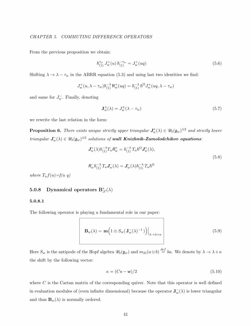
5.0.8.1
The following operator is playing a fundamental role in our paper:
Bw(λ) = m(1⊗ Sw(J−w(λ)−1 )
)∣∣∣λ→λ+κ
(5.9)
Here Sw is the antipode of the Hopf algebra U~(gw) and m21(a⊗b)def= ba. We denote by λ→ λ+κ
the shift by the following vector:
κ = (Cv − w)/2 (5.10)
where C is the Cartan matrix of the corresponding quiver. Note that this operator is well defined
in evaluation modules of (even infinite dimensional) because the operator J−w(λ) is lower triangular
and thus Bw(λ) is normally ordered.
41

CHAPTER 5. COMMUTING DIFFERENCE OPERATORS
5.0.8.2
Let L ∈ Pic(X) be a line bundle. Let us fix a slope s ∈ H2(X,R) and choose a path p in H2(X,R)
from s to s−L . We assume that this path positively crosses finitely many walls in the following
order w1, w2, ..., wm. For this choice of slope and a line bundle we associate the following operator:
BsL (λ) = LBwm(λ) · · ·Bw1(λ) ∈ U~(gQ) (5.11)
In this formula L denotes the operator of multiplication by a line bundle in KG(X). We will also
define the q-difference operators:
A sL = T−1L Bs
L (λ)
where the notations are same as in Section 5.0.6.1.
5.0.8.3
Let Rs(u) be the slope s R-matrix. We define the quantum Knizhnik-Zamolodchikov operator
acting in the space KG(XA)-valued functions explicitly:
K s = ~λ(1)T−1u Rs(u) (5.12)
where Tuf(u) = f(uq) is a q-difference operator.
Theorem 4. Let s, s′ be two slopes separated by a single wall w, then the corresponding q-difference
operators are conjugated:
W−1K sW = K s′ , W−1A sLW = A s′
L (5.13)
where W = Bw(λ)(R+w)−1 and we assume that passing from s to s′ we cross the wall w in the
positive direction. .
As a consequence of this theorem we will prove the following result:
Corollary 3. 1) The operator BsL (λ) does not depend on the choice of path from in (5.11).
2) The q-difference operators commute for all L ,L ′ ∈ Pic(X) and s ∈ H2(X,R):
A sL A s
L ′ = A sL ′A
sL , A s
L K sL = K s
L A sL
42
CHAPTER 5. COMMUTING DIFFERENCE OPERATORS
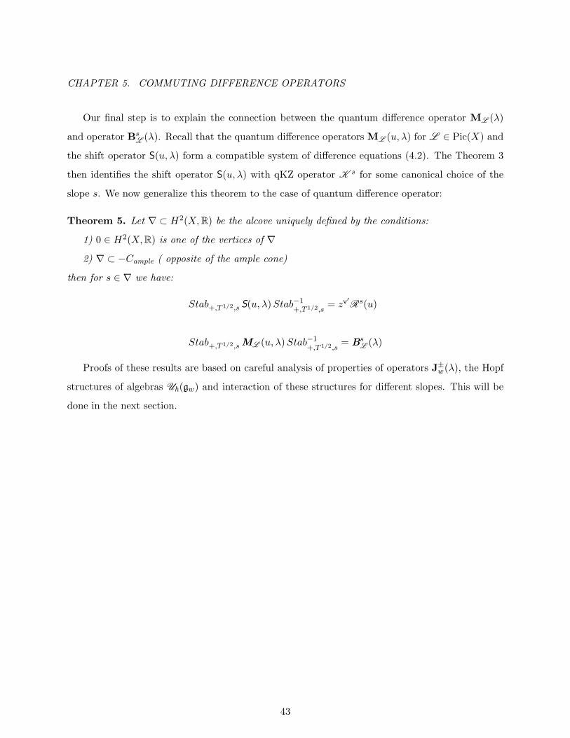
Our final step is to explain the connection between the quantum difference operator ML (λ)
and operator BsL (λ). Recall that the quantum difference operators ML (u, λ) for L ∈ Pic(X) and
the shift operator S(u, λ) form a compatible system of difference equations (4.2). The Theorem 3
then identifies the shift operator S(u, λ) with qKZ operator K s for some canonical choice of the
slope s. We now generalize this theorem to the case of quantum difference operator:
Theorem 5. Let ∇ ⊂ H2(X,R) be the alcove uniquely defined by the conditions:
1) 0 ∈ H2(X,R) is one of the vertices of ∇
2) ∇ ⊂ −Cample ( opposite of the ample cone)
then for s ∈ ∇ we have:
Stab+,T 1/2,s S(u, λ)Stab−1+,T 1/2,s
= zv′Rs(u)
Stab+,T 1/2,sML (u, λ)Stab−1+,T 1/2,s
= BsL (λ)
Proofs of these results are based on careful analysis of properties of operators J±w(λ), the Hopf
structures of algebras U~(gw) and interaction of these structures for different slopes. This will be
done in the next section.
43

CHAPTER 6. PROOFS OF THEOREMS ?? AND ??
Chapter 6
Proofs of Theorems 4 and 5
6.1 Cocycle identity
In this section we prove that the solutions of ABRR equations satisfy dynamical cocycle identities.
Our presentation follows closely to [11] where this fact was fist proven for simple quantized Lie
algebras.
6.1.1
Let J±w (λ) be the operators defined by Proposition 5. Let us denote J±(λ)12 = J±w (λ)⊗1, J±(λ)23 =
1 ⊗ J±w (λ), J±(λ)12,3 = (∆w ⊗ 1)J±w (λ), J±(λ)1,23 = (1 ⊗ ∆w)J±w (λ) the operators in U~(gw) ⊗
U~(gw)⊗U~(gw). Then we have:
Theorem 6. The operators J±(λ) satisfy the dynamical cocycle conditions:
J−(λ)12,3J−(λ+ κ(3))12 = J−(λ)1,23J−(λ− κ(1))23
J+(λ+ κ(3))12J+(λ)12,3 = J+(λ− κ(1))23J+(λ)1,23
(6.1)
with dynamical shift κ = (Cv − w)/2 where C is the Cartan matrix of the quiver.
We will need the three-component analog of Proposition 5. We start with definition of up-
per/lower triangular operators acting in a tensor product of three U~(gw) modules. Let X =
44

CHAPTER 6. PROOFS OF THEOREMS ?? AND ??
M (v,w) - be a Nakajima variety, and let A be a torus splitting the framing such that:
XA =⨿
v1+v2+v3=v
M (v1,w1)×M (v2,w2)×M (v3,w3). (6.2)
We say that the operator A ∈ End(KT(XA)) is upper triangular if A =
⊕⟨α,θ⟩>0⟨β,θ⟩<0
Aα,β where θ is the
stability parameter of the Nakajima variety and:
Aα,β : KT(M (v1,w1)×M (v2,w2)×M (v3,w3))→
KT(M (v1 + α,w1)×M (v2 + γ,w2)×M (v3 + β,w3))
Obviously, γ is defined from the condition α+β+γ = 0. Similarly, the operator is lower triangular
if A =⊕⟨α,θ⟩<0⟨β,θ⟩>0
Aα,β with the same Aα,β as above. Finally, we say that an operator is strictly upper or
lower triangular if, in addition, A0,0 = 1. For example, the product of wall R-matrices R+,13w R+,12
w
or R+,13w R+,23
w (where the indices indicate in which components of (6.2) they act), are strictly upper
triangular.
In the three-component case we have two types of qKZ operators ~λ(3)R+,13w R+,23
w and ~−λ(1)R+,13w R+,12
w
which correspond to the coproducts of the wall qKZ operators in the first or the second component.
Proposition 7. If there exists a strictly upper triangular operator J(λ) ∈ End(KT(XA)) satisfying:
J(λ) ~λ(3)R+,13w R+,23
w = ~λ(3)~Ω13+Ω23 J(λ)
J(λ) ~−λ(1)R+,13w R+,12
w = ~−λ(1)~Ω13+Ω12 J(λ)
(6.3)
or strictly lower-triangular operator J(λ) ∈ End(KT(XA)) satisfying
R−,23w R−,13w ~λ(3)J(λ) = J(λ)~Ω23+Ω13 ~λ(3)
R−,12w R−,13w ~−λ(1) J(λ) = J(λ)~Ω12+Ω13 ~−λ(1)
then it is unique.
Proof. We prove the upper-triangular case. The lower-triangular case is similar. Following [13] we
45

CHAPTER 6. PROOFS OF THEOREMS ?? AND ??
introduce the operators:
AR(X) = ~−Ω13−Ω23~−λ(3)X~λ(3)R+,13w R+,23
w ,
AL(X) = ~−Ω13−Ω12~λ(1)X~−λ(1)R+,13w R+,12
w
Assume that there exist operator J(λ) satisfying conditions of the proposition. Then, obviously
ARAL(J(λ)) = J(λ). It is enough to check that the solution for this equation is unique. We are
given that J(λ) =⊕⟨α,θ⟩>0⟨β,θ⟩<0
Jα,β(λ), and thus this equation has the following form in components:
Jα,β(λ) = Ad~λ(1)
~−λ(3)
~−Ω
(Jα,β(λ)
)+ · · · (6.4)
where Ω = 2Ω13 +Ω23 +Ω12 and · · · stands for the lower terms Jα′,β′(λ) with
⟨α′ − β′, θ⟩ < ⟨α− β, θ⟩
Note that the operator 1−Ad~λ(1)
~−λ(3)
~−Ω is invertible for generic λ. This means that all Jα,β(λ) can
be expressed trough the lowest term J0,0(λ) = 1 and therefore they are uniquely determined by
(6.4).
Let J(λ) be as in Proposition 5. It is obvious that J+(λ + κ(3))12J+(λ)12,3 is a solution of
AR(X) = X. Similarly J+(λ − κ(1))23J+(λ)1,23 is the solution of AL(X) = X. Thus, by the
previous proposition, to prove Theorem 6 it is enough to prove the following lemma:
Lemma 1.
X = J+(λ+ κ(3))12J+(λ)12,3 is a solution of AL(X) = X
X = J+(λ− κ(1))23J+(λ)1,23 is a solution of AR(X) = X
Proof. 1) As noted above the element X = J+(λ + κ(3))12J+(λ)12,3 is a solution of AR(X) = X.
Note, that AR and AL commute (due to Yang-Baxter equation for R+w). Thus, Y = AL(X) is also
a solution of this equation. The solution of AR(X) = X is uniquely determined by the degree zero
part in the third component. Denote this comportment of X by X0 and similarly for Y by Y0.
Enough to prove that X0 = Y0. For X0 we obtain:
X0 = J+(λ+ κ(3))12
46

CHAPTER 6. PROOFS OF THEOREMS ?? AND ??
For Y0 we have:
Y0 = ~−Ω13−Ω12~λ(1)J+(λ+ κ(3))
12 ~−λ(1)~Ω13R+,12
w (6.5)
Denote by Z = J+(λ+ κ(3))12. By triangularity of R-matrix and J(λ) it factors Z =
⊕α∈NI
Zα with:
Zα : KG
(M (v1,w1)×M (v2,w2)×M (v3,w3)
)
→ KG
(M (v1 + α,w1)×M (v2 − α,w2)×M (v3,w3)
)Thus, by definition of codimension function (2.27) we have ~−Ω13Zα~Ω13 = ~mαZα where
mα =
12
(⟨v1,w3⟩+ ⟨v3,w1⟩ − ⟨v1, Cv3⟩
)− 1
2
(⟨v1 + α,w3⟩+ ⟨v3,w1⟩ − ⟨v1 + α,Cv3⟩
)
= ⟨α, κ(3)⟩
with κ(3) = (Cv3 − w3)/2. Therefore, using the dynamical notations we can write the equation
(6.5) in the form:
Y0 = ~−Ω12~λ+κ(3)
(1) J+(λ+ κ(3))12 ~−λ−κ(3)
(1) R+,12w
As J+(λ) is satisfies condition of Proposition 5 we obtain Y0 = J+(λ+ κ(3))12. Therefore Y = X.
The second equality is proved analogously.
6.2 Coproduct of Bw(λ)
6.2.1
Let us consider the operators:
B′w(λ) = m(1⊗ Sw(J−w (λ)−1)
), B′w(λ) = m21
(S−1w ⊗ 1(J−w (λ)−1)
)where Sw is the antipode of U~(gw) and m(a⊗ b) def
= ab, m21(a⊗ b)def= ba. We define:
Bw(λ) = B′w(λ+ κ), Bw(λ) = B′w(λ− κ) (6.6)
with κ as in the Theorem 6. Then, we have:
47
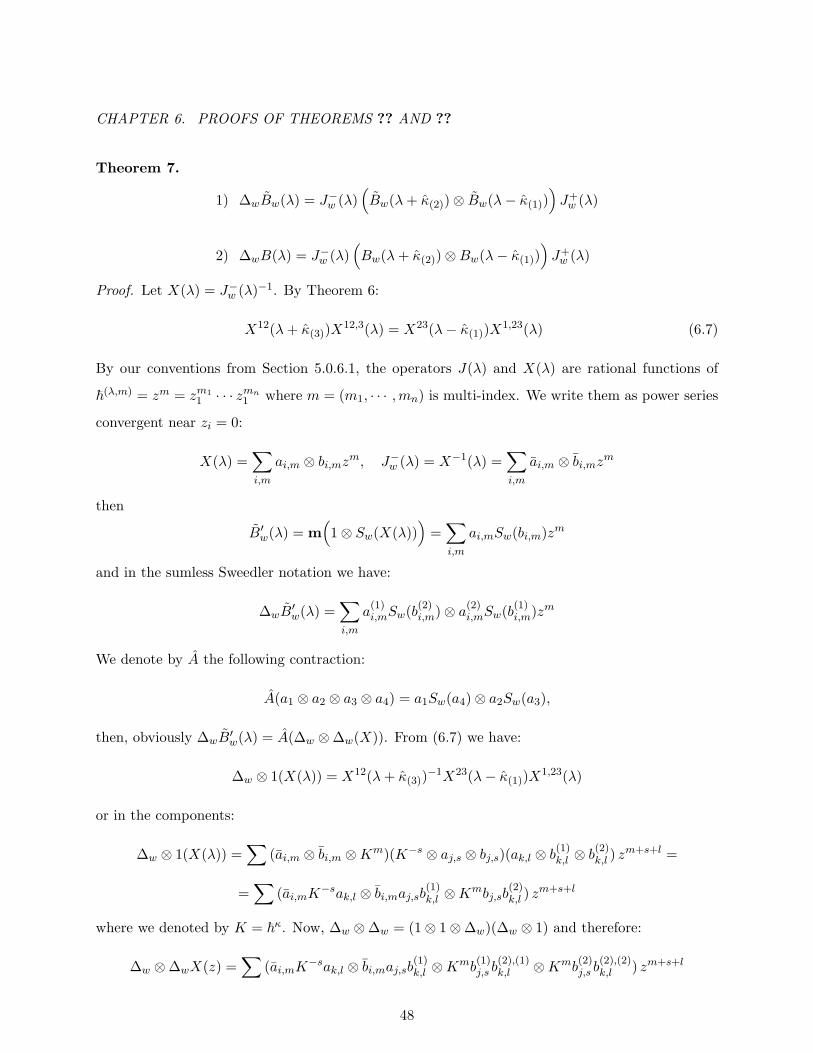
CHAPTER 6. PROOFS OF THEOREMS ?? AND ??
Theorem 7.
1) ∆wBw(λ) = J−w (λ)(Bw(λ+ κ(2))⊗ Bw(λ− κ(1))
)J+w (λ)
2) ∆wB(λ) = J−w (λ)(Bw(λ+ κ(2))⊗Bw(λ− κ(1))
)J+w (λ)
Proof. Let X(λ) = J−w (λ)−1. By Theorem 6:
X12(λ+ κ(3))X12,3(λ) = X23(λ− κ(1))X1,23(λ) (6.7)
By our conventions from Section 5.0.6.1, the operators J(λ) and X(λ) are rational functions of
~(λ,m) = zm = zm11 · · · zmn
1 where m = (m1, · · · ,mn) is multi-index. We write them as power series
convergent near zi = 0:
X(λ) =∑i,m
ai,m ⊗ bi,mzm, J−w (λ) = X−1(λ) =∑i,m
ai,m ⊗ bi,mzm
then
B′w(λ) = m(1⊗ Sw(X(λ))
)=∑i,m
ai,mSw(bi,m)zm
and in the sumless Sweedler notation we have:
∆wB′w(λ) =
∑i,m
a(1)i,mSw(b
(2)i,m)⊗ a(2)i,mSw(b
(1)i,m)zm
We denote by A the following contraction:
A(a1 ⊗ a2 ⊗ a3 ⊗ a4) = a1Sw(a4)⊗ a2Sw(a3),
then, obviously ∆wB′w(λ) = A(∆w ⊗∆w(X)). From (6.7) we have:
∆w ⊗ 1(X(λ)) = X12(λ+ κ(3))−1X23(λ− κ(1))X1,23(λ)
or in the components:
∆w ⊗ 1(X(λ)) =∑
(ai,m ⊗ bi,m ⊗Km)(K−s ⊗ aj,s ⊗ bj,s)(ak,l ⊗ b(1)k,l ⊗ b
(2)k,l ) z
m+s+l =
=∑
(ai,mK−sak,l ⊗ bi,maj,sb
(1)k,l ⊗K
mbj,sb(2)k,l ) z
m+s+l
where we denoted by K = ~κ. Now, ∆w ⊗∆w = (1⊗ 1⊗∆w)(∆w ⊗ 1) and therefore:
∆w ⊗∆wX(z) =∑
(ai,mK−sak,l ⊗ bi,maj,sb
(1)k,l ⊗K
mb(1)j,s b
(2),(1)k,l ⊗Kmb
(2)j,s b
(2),(2)k,l ) zm+s+l
48

CHAPTER 6. PROOFS OF THEOREMS ?? AND ??
Applying contraction A, taking into account that antipode Sw is antihomomorphism and Sw(K) =
K−1 by (3.8) we obtain:
A(∆w ⊗∆wX) =
∑ai,mK
−sak,lSw(b(2),(2)k,l )Sw(b
(2)j,s )K
−m ⊗ bi,maj,sb(1)k,lSw(b(2),(1)k,l )Sw(b
(1)j,s )K
−m zm+s+l
= J−w (λ− κ(1) − κ(2))∑
K−sak,lSw(b(2),(2)k,l )Sw(b
(2)j,s )⊗ aj,sb
(1)k,lSw(b
(2),(1)k,l )Sw(b
(1)j,s ) z
s+l
where J−w (λ− κ(1)− κ(2)) =∑
ai,mK−m⊗ bi,mK−mzm and in the last step we used that the whole
operator is weight zero and therefore commutes with K ⊗ K. From the simple Lemma (2) we
obtain:
A(∆w ⊗∆wX(λ)) =
J−w (λ− κ(1) − κ(2))∑
K−sak,lSw(bk,l)Sw(b(2)j,s )⊗ aj,sSw(b
(1)j,s ) z
s+l =
J−w (λ− κ(1) − κ(2))B′w(λ)⊗ 1 ·(∑
K−sSw(b(2)j,s )⊗ aj,sSw(b
(1)j,s ) z
s)
Let us consider the contraction defined by P (a1 ⊗ a2 ⊗ a3) = Sw(a3) ⊗ a1Sw(a2). Then for the
expression in the brackets in the last formula we have:
∑K−sSw(b
(2)j,s )⊗ aj,sSw(b
(1)j,s ) z
s = P(X1,23(λ+ κ(3))
)Again, by from (6.7) we have:
X1,23(λ+ κ(3)) = X23(λ− κ(1) + κ(3))−1X12(λ+ 2κ(3))X
12,3(λ+ κ(3))
=∑
K−maj,sa(1)k,l ⊗ ai,mbj,sa
(2)k,l ⊗ bi,mK
m+2sbk,lKlzs+m+l.
Thus
P(X1,23(λ+ κ(3))
)=
∑K−lSw(bk,l)K
−m−2sSw(bi,m)⊗K−maj,sa(1)k,lS(a(2)k,l )Sw(bj,s)Sw(ai,m)zs+m+l
49

CHAPTER 6. PROOFS OF THEOREMS ?? AND ??
Note, that a(1)k,lSw(a
(2)k,l ) = ϵw(ak,l), and using the unipotence of J−w (λ) we find:
P(X1,23(λ+ κ(3))
)=∑K−m−2sSw(bi,m)⊗K−maj,sSw(bj,s)Sw(ai,m)zs+m
=(∑
K−2s ⊗ aj,sSw(bj,s)zs)(∑
K−mSw(bi,m)⊗K−mSw(ai,m)zm)
=(1⊗ B′w(λ− 2κ(1))
)Sw ⊗ Sw((J+
w )21)(λ− κ(1) − κ(2))
Overall we obtain the identity:
∆wB′(λ) = J−w (λ− κ(1) − κ(2))
(B′w(λ)⊗ B′w(λ− 2κ(1))
)Sw ⊗ Sw((J−w )21)(λ− κ(1) − κ(3))
Finally, after shifting λ→ λ+ κ(1)+ κ(2) and using (5.4) we obtain 1). The equation 2) is obtained
similarly.
Lemma 2.
∑S(x(2),(2))⊗ x(1)S(x(2),(1)) = S(x)⊗ 1 (6.8)
Proof. Consider the contraction C(a1 ⊗ a2 ⊗ a3) = S(a3)⊗ a1S(a2) then, obviously∑S(x(2),(2))⊗ x(1)S(x(2),(1)) = C
(1⊗∆(∆x)
)= C
(∆⊗ 1(∆x)
)
= S(x(2))⊗ x(1)(1)S(x(1)(2)) = S(x(2))⊗ ϵ(x(1)) = S(x)⊗ 1
6.2.2
Corollary 4. The coproduct of the operator Bw(λ) defined by (5.9), has the following form:
∆w(Bw(λ)) = J−w(λ)(Bw(λ+ κ(2))⊗Bw(λ− κ(1))
)J+w(λ) (6.9)
Proof. Shift λ→ λ− τw and use definitions (5.7) and (5.9).
50

CHAPTER 6. PROOFS OF THEOREMS ?? AND ??
6.3 Other properties of Bw(λ)
6.3.1
Let us consider the wall qKZ operators as in the Proposition 6:
K +w = Tu~−λ(1)R
+w , K −
w = R−wTu~−λ(1) (6.10)
acting in the tensor product of two evaluation modules of U~(gQ).
Proposition 8.
K −w ∆w(Bw(λ)) = ∆w(Bw(λ))K +
w (6.11)
Proof. We have
K −w ∆w(Bw(λ))
(6.9)=
R−wTu~−λ(1)J−w(λ)
(Bw(λ+ κ(2))⊗Bw(λ− κ(1))
)J+w(λ)
(5.8)=
J−w(λ)Tu~−λ(1)~Ω(Bw(λ+ κ(2))⊗Bw(λ− κ(1))
)J+w(λ) =
J−w(λ)(Bw(λ+ κ(2))⊗Bw(λ− κ(1))
)Tu~−λ(1)~
ΩJ+w(λ)
(5.8)=
J−w(λ)(Bw(λ+ κ(2))⊗Bw(λ− κ(1))
)J+w(λ)~−λ(1)TuR
+w =
∆w(Bw(λ))K +w
6.3.2
Proposition 9. For L ∈ Pic(X) the operators Bw(λ) satisfy:
L T−1L Bw(λ) = Bw+L (λ)L T−1L (6.12)
with shift operators TL defined by (5.2).
51

CHAPTER 6. PROOFS OF THEOREMS ?? AND ??
Proof. Let A be a torus splitting the framing w = u′w′ + u′′w′′. We a consider Nakajima variety
X = M (v,w). The components of XA are of the form Fi = M (v′i,w′)×M (v′′i ,w
′′). Let us consider
the operators:
SC,s = i∗XA StabC,T 1/2,s : KG(XA) −→ KG(X
A)
where iXA is the inclusion map. Let L ∈ Pic(X) be a line bundle. We denote by U(L ) a block
diagonal operator acting in KG(XA) with the following matrix elements:
U(L )|Fi×Fi= L |Fi
Let us consider an operator SC,s = U(L )SC,sU(L )−1. A conjugation by a diagonal matrix does
not change the diagonal elements, thus:
SC,s∣∣Fi×Fi
= SC,s|Fi×Fi(6.13)
For the non-diagonal elements we have:
degA
(SC,s
∣∣F2×F1
)= degA
(SC,s|F2×F1
L |F2
L |F1
)
(2.5)⊂ degA
(SC,s|F2×F2
s⊗L |F2
s⊗L |F1
)(6.13)= degA
(SC,s
∣∣F2×F2
s⊗L |F2
s⊗L |F1
) (6.14)
Note, that the stable map is defined uniquely by these restrictions and thus we conclude: SC,s =
SC,s+L .
Recall that the wall R-matrices are defined by R±w = S−1±,s2S±,s1 for two slopes s1 and s2
separated by a single wall w. Therefore:
U(L )R±wU(L )−1 = R±w+L .
Conjugating both sides of ABRR equation (5.3) by U(L ) we get:
R−w+L ~−λ(1)U(L )J−w (λ)U(L )−1 = U(L )J−w (λ)U(L )−1~−λ(1) ~Ω
Thus, by uniqueness of the solution of this equation:
U(L )J−w (λ)U(L )−1 = J−w+L (λ) (6.15)
52

CHAPTER 6. PROOFS OF THEOREMS ?? AND ??
Without a loss of generality we can assume that L = det(Vk) is the k-th tautological line bundle.
Then, we have:
U(L ) = L ⊗ L
Where L is the same tautological bundle twisted by some powers of trivial line bundles u′ and u′′:
explicitly for the component F = M (v′,w′)×M (v′′,w′′) we have: L |F = (u′)v′kL ⊗ (u′′)v
′′kL .
Let (J−w (λ))−1 =∑
i ai ⊗ bi, (J−w+L (λ))−1 =
∑i a′i ⊗ b′i. and denote by Bw(λ) =
∑i aiSw(bi).
Then we have:
LBw(λ)L −1 = LBw(λ)L −1 =∑
i L aiSw(L ai) =
m(1⊗ Sw(
∑i L ai ⊗ L bi)
)(6.15)= m
(1⊗ Sw(
∑i a′iL ⊗ b′iL )
)
=∑
i a′iSw(b
′i) = Bw+L (λ).
In the first equality we substituted L by L because for one component case the u-factors cancels.
Thus we proved that:
LBw(λ) = Bw+L (λ)L
Finally, note that Bw(λ) = Bw(λ+ τw) and thus:
LBw(λ+ τw) = Bw+L (λ+ τw+L )L
By definition τw+L − τw = sL thus, after substitution λ→ λ− τw − sL we obtain:
LBw(λ− sL ) = Bw+L (λ)L
which gives (6.12).
6.4 Proof of Theorem 4
6.4.1
We have
K s = ~λ(1)T−1u Rs(u), K s′ = ~λ(1)T
−1u Rs′(u), W = ∆w(Bw(λ))(R
+w)−1.
53

CHAPTER 6. PROOFS OF THEOREMS ?? AND ??
We need to check that K sW =WK s′ . We have:
K sW = ~λ(1)T−1u Rs(u)∆w(Bw(λ))(R
+w)−1 =
~λ(1)T−1u ∆op
w (Bw(λ))Rs(u)(R+w)−1 =
~λ(1)T−1u (R−)−1R−∆op
w (Bw(λ))Rs(u)(R+w)−1 =
~λ(1)T−1u (R−)−1∆w(Bw(λ))~ΩR−wRs(u)(R+
w)−1 (6.11)
=
∆w(Bw(λ))(R+w)−1~λ(1)T
−1u R−wRs(u)(R+
w)−1 =WK s′
where the last equality uses Rs′(u) = R−wRs(u)(R+w)−1 because by assumption s and s′ are sepa-
rated by a single wall w.
6.4.2
The following proposition describes the action of the difference operator A sL in the tensor product
of two U~(gQ) modules.
Proposition 10.
∆s(AsL ) =Ww0(λ)Ww1(λ) · · ·Wwm−1(λ)∆∞(L )T−1L
where w0, · · · , wm−1 is the ordered set of walls separating line bundles s and s + L , Ww(λ) =
∆w(Bw(λ))(R+w)−1 and ∆∞ is the infinite slope coproduct from Section 3.3.5.
Proof. First, by definition (5.11) we have:
A sL = T−1L L Bw−m(λ)Bw−2(λ) · · ·Bw−1(λ)
Where, we denote by w−1, · · ·w−m the ordered set of walls between the slope s and s − L . By
Proposition 9 we know that T−1L LBwk(λ) = Bwk+m
(λ)T−1L L and thus we obtain:
A sL = Bw0(λ)Bw1(λ) · · ·Bwm(λ)L T−1L
with walls wi as in the proposition.
54

CHAPTER 6. PROOFS OF THEOREMS ?? AND ??
Next, for coproduct we have:
∆s(AsL ) = ∆s(Bw0(λ)Bw1(λ) · · ·Bwm(λ)L )T−1L
and by (3.6) the coproducts at different slopes are related as follows
∆s(Bwk(λ)) = (R+
w0)−1 · · · (R+
wk−1)−1∆wk
(Bwk)R+
wk−1· · ·R+
w0.
Thus we obtain:
A sL = ∆w0(Bw0(λ))(R
+w0)−1 · · ·∆wm(Bwm(λ))(R
+wm
)−1R+wm· · ·R+
w0∆s(L )T−1L
The proposition follows from next Lemma.
Lemma 3. Let w0, · · · , wm be the ordered set of walls between s and s+ L . Then we have:
∆∞(L ) = R+wm· · ·R+
w0∆s(L ) (6.16)
Proof. By (3.6) the coproducts are related as follows:
∆s(L ) = (R+w0)−1 · · · (R+
∞)−1∆∞(L )R+∞ · · ·R+
w0
By definition ∆∞(L ) = L ⊗L . In particular,
∆∞(L )R+wk
∆∞(L )−1 = R+wk+L = R+
wk+m
We use this identity to cancel all but finitely many factors in the previous expression. The lemma
is proven.
6.4.3
Let s and s′ be two slopes separated by a single wall w0. We choose a path from slope s to s+ L
crossing some sequence of walls w0, w1..., wm. Similarly, for the path from s′ to s′ −L crosses the
walls w1, w2..., wm+1 with wm = w0 + L . By Proposition 10 we have:
∆s(A sL ) =Ww0(λ) · · ·Wwm(λ)∆∞(L )T−1L
∆s′(As′L ) =Ww1(λ) · · ·Wwm+1(λ)∆∞(L )T−1L
To finish the proof of the Theorem 4 we need to check that
Ww0(λ)−1∆s(A
sL )Ww0(λ) = ∆s′(A
s′L ).
But this is obvious.
55

CHAPTER 6. PROOFS OF THEOREMS ?? AND ??
6.5 Proof of Corollary 3
In fact, the statement of the Corollary 3 follows immediately from Proposition 10. Indeed, we
obtain
K s∆s(A sL ) = K sWw0(λ)Ww1(λ) · · ·Wwn(λ)∆∞(L )T−1L
(5.13)=
Ww0(λ)Ww1(λ) · · ·Wwn(λ)Ks+L∆∞(L )T−1L = ∆s(A s
L )K s
However, in this section we will consider alternative proof. The Theorem 4 says that the difference
operators for different choices of slopes are conjugated. Thus, to prove the commutativity it is
enough to check it for some particular slope. The natural choice is the “infinite” slope. The aim
of this section is to illustrate the general principle: at the infinite slope the difference operators
become trivial and the commutativity is obvious.
6.5.1
First, by Theorem 4 we have XA sLX
−1 = A∞L where X is a product of wall operators W . As
A∞L does not depend on the choice of a path (its exact form is established in the next section) we
conclude that A sL does not depend on this choice.
6.5.2
To compute A∞L we use the following proposition.
Proposition 11. If J−w (λ) is the strictly lower-triangular solution of ABRR equation then:
limλ→−∞
J−w (λ) = 1
Proof. By definition, the limit λ→ −∞ means that λ goes to infinity in the opposite ample cone.
For a Nakajima variety the line bundle corresponding to the stability parameter θ ∈ ZI is ample.
Thus we need to prove that for λ = xθ and x ∈ R we have:
limx→−∞
J−w (xθ) = 1
As the operator J−w is strictly lower-triangular, this is equivalent to:
limx→−∞
J−w (xθ)α = 0 for α = 0
56

CHAPTER 6. PROOFS OF THEOREMS ?? AND ??
We prove it by induction on the value of ⟨α, θ⟩. The ABRR equation takes the form:
~−xθ(1) J−w (xθ)~xθ(1) = (R−w)
−1J−w (xθ)~Ω
or, in the components:
J−w (xθ)α~−x⟨α,θ⟩ = J−w (xθ)α + lower terms
where the lower terms are J−w (xθ)α′ with ⟨α′, θ⟩ > ⟨α, θ⟩. Therefore:
limx→−∞
J−w (xθ)α = limx→−∞
1
~−x⟨α,θ⟩ − 1
(lower terms
)By induction, the lower terms vanish in this limit. By lower-trianguality of J−w (λ) we have ⟨α, θ⟩ < 0,
thus the prefactor vanishes as well.
Corollary 5.
A∞L = L T−1L (6.17)
Proof. To compute the operator BsL (λ) at the infinite slope s = ∞ we note that all walls that
contribute to the product (5.11) correspond to τw →∞. By definition (5.7) we have:
limτw→∞
J−w(λ) = limτw→∞
J−w (λ− τw) = 1
where the second equality is by previous proposition. By (5.9) we obtain limτw→∞
Bw(λ) = 1.
Now, it is obvious that the operators A∞L commute among themselves. But, by Theorem 4 it
means that they commute for arbitrary slope
[A sL ,A
sL ′ ] = 0.
6.5.3
Let A be a torus splitting the framing w = uw′+w′′. Let K ∞ = ~λ(1)T−1u R∞(u) be the corresponding
qKZ operator with infinite slope acting in KG(M (w′))⊗KG(M (w′′)). By the previous section the
operator A∞L acts on this space by A∞L = ∆∞(L )T−1L . Without a loss of generality we assume
that L = det(Vk) is the k-th tautological line bundle. The coproduct at the infinite slope splits,
meaning that ∆∞(L ) = L ⊗L .
57

CHAPTER 6. PROOFS OF THEOREMS ?? AND ??
The R-matrix R∞(u) is the operator of multiplication by class (2.24) in the equivariant K-
theory. Therefore, R∞(u) commutes with ~λ(i) and the operators of multiplication by ∆∞(L ). We
need to check that K ∞A∞L = A∞L K ∞ which therefore means:
∆∞(L )T−1zk(~λ(1)) = ~λ(1) T
−1u (∆∞(L )) (6.18)
and follows from definition of ~λ(1).
6.6 Proof of Theorem 5
6.6.1
Let A = C× be a torus splitting the framing space as w = uw′ + w′′ and acting on a Nakajima
variety X = M (v,w). We denote the components of XA by Fv′ = M (v′,w′) ×M (v′′,w′′). Note,
that we label them by the weight in the first component. For a line bundle L we have two difference
operators acting in KG(w′)⊗KG(w
′′) and commuting with the qKZ operator K s for a slope s as
in the Theorem 5. First, by Theorem 3:
AL = T−1L NsL (u, λ)
for NsL (u, λ) = Stab+,T 1/2,s ML (u, λ) Stab−1
+,T 1/2,scommutes with qKZ operator at the slope s.
Second, by the corollary of Theorem 4, the operator:
AL = T−1L BsL (u, λ)
commutes with the same qKZ operator. We prove that they coincide up to a constant multiple:
BsL (u, λ) = Ns
L (u, z)Const
6.6.2
Both NL (u, z) and BsL (u, z) are defined in integral K-theory, in particular they and their inverses
are Laurent polynomials in u. It follows that the operator:
U(u) = BsL (u, z)N−1L (u, z)
58

CHAPTER 6. PROOFS OF THEOREMS ?? AND ??
is a Laurent polynomial in u. By construction, this operator commutes with qKZ at a slope s which
means that:
U(uq) = ~λ(1)Rs(u)U(u)
(~λ(1)R
s(u))−1
From Khoroshkin-Tolstoy factorization for the slope s R-matrix we obtain:
Rs(0) = ~−Ω←∏0∈w
R+w Rs(∞) =
→∏0∈w
(R−w)−1 ~Ω
where R+w and R−w are strictly upper and lower triangular wall R-matrixes. The products run over
walls passing through 0 ∈ H2(X,R). Therefore, the eigenvalues of conjugation by ~λ(1)Rs(u) at
u = 0,∞ are either 1 or zm~m′ with m = 0. Solutions in Laurent series in u thus necessarily
correspond to eigenvalue 1. In particular, they are regular at u = 0 and u =∞. It follows that U
is a constant matrix in u.
6.6.3
The constant matrix U commutes with ~λ(1)Rs(u). Diagonalizing the matrix ~λ(1)R
s(0) we find that
U is upper triangular. Similarly diagonalizing ~λ(1)Rs(∞) we find that U is block lower triangular.
We conclude that U is block diagonal matrix.
Let us consider the diagonal block U0,0 of the matrix U corresponding to the lowest component
of the fixed point set:
U0,0 : KG(F0)→ KG(F0)
Since U commutes with qKZ, the block U0,0 commutes with the corresponding block of R-matrix
Rs0,0(u). From definition of R-matrix the matrix element Rs
0,0(u) is the generating function for
operators of classical multiplication by tautological classes on F0. Thus, the operator U0,0 is itself
an operator of multiplication by some class in KG(F0). To finish the proof it remain to note that:
U0,0 = UF0 (6.19)
Where UF0 denotes the same operator U for quiver variety F0. Indeed, applying (6.19) to X in place
of F0 we conclude, that U is an operator of multiplication in KG(X). However, so such nonscalar
operator can be diagonal in the stable basis. We conclude that U = Const.
59
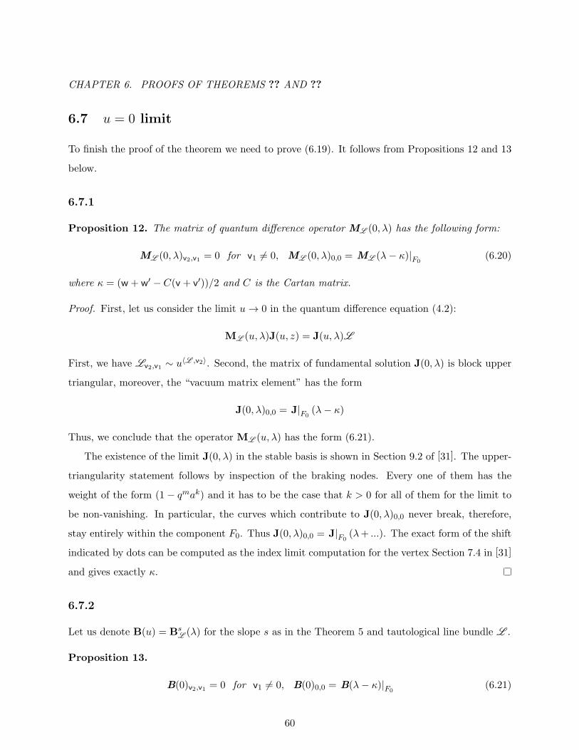
CHAPTER 6. PROOFS OF THEOREMS ?? AND ??
6.7 u = 0 limit
To finish the proof of the theorem we need to prove (6.19). It follows from Propositions 12 and 13
below.
6.7.1
Proposition 12. The matrix of quantum difference operator ML (0, λ) has the following form:
ML (0, λ)v2,v1 = 0 for v1 = 0, ML (0, λ)0,0 = ML (λ− κ)|F0(6.20)
where κ = (w + w′ − C(v + v′))/2 and C is the Cartan matrix.
Proof. First, let us consider the limit u→ 0 in the quantum difference equation (4.2):
ML (u, λ)J(u, z) = J(u, λ)L
First, we have Lv2,v1 ∼ u⟨L ,v2⟩. Second, the matrix of fundamental solution J(0, λ) is block upper
triangular, moreover, the “vacuum matrix element” has the form
J(0, λ)0,0 = J|F0(λ− κ)
Thus, we conclude that the operator ML (u, λ) has the form (6.21).
The existence of the limit J(0, λ) in the stable basis is shown in Section 9.2 of [31]. The upper-
triangularity statement follows by inspection of the braking nodes. Every one of them has the
weight of the form (1− qmak) and it has to be the case that k > 0 for all of them for the limit to
be non-vanishing. In particular, the curves which contribute to J(0, λ)0,0 never break, therefore,
stay entirely within the component F0. Thus J(0, λ)0,0 = J|F0(λ+ ...). The exact form of the shift
indicated by dots can be computed as the index limit computation for the vertex Section 7.4 in [31]
and gives exactly κ.
6.7.2
Let us denote B(u) = BsL (λ) for the slope s as in the Theorem 5 and tautological line bundle L .
Proposition 13.
B(0)v2,v1 = 0 for v1 = 0, B(0)0,0 = B(λ− κ)|F0(6.21)
60

CHAPTER 6. PROOFS OF THEOREMS ?? AND ??
Proof. 6.7.3
First by Proposition 10, in the tensor product of two U~(gQ) modules we have:
B(u) =Ww0(λ)Ww1(λ) · · ·Wwn−1(λ)∆∞(L ) (6.22)
where Ww(λ) = ∆w(Bw)(R+w)−1 and w0, · · ·wn−1 is the ordered set of walls crossed by an interval
from s to s+ L .
6.7.4
By Corollary 6.9 we have:
∆w(Bw(λ)) = J−w(λ)(Bw(λ+ κ(2))⊗Bw(λ− κ(1))
)J+w(λ)
Recall, that the operators J−w(λ) and R+w are triangular with the following matrix elements:
J±w(λ) =
∞⊕s=0,
±⟨α,θ⟩>0
Jsα, R±w(λ) =
∞⊕s=0,
±⟨α,θ⟩>0
Rsα
where θ is the stability parameter of the quiver and α is the root defining the wall w:
w = x ∈ H2(X,R)|⟨x, α⟩ = m.
The matrix elements are of the form:
Jsα, Rsα : KG(Fv) −→ KG(Fv+sα)
and by Theorem 1 they have the following dependence on the equivariant parameter u:
Jsα, Rsα ∼ us⟨α,Lw⟩.
where Lw is a line bundle on the wall w. We conclude that the matrix elements of Ww(λ) have the
following form:
Ww(λ)v2,v1 ∼ u⟨sα,Lw⟩, if v2 = v1 + sα. (6.23)
61

CHAPTER 6. PROOFS OF THEOREMS ?? AND ??
6.7.5
From (6.22) we see that the matrix element B(1)v2,v1 has takes the form:
Bv2,v1 =
∞∑s0,··· ,sn−1=0
Bv2,v1(s0, · · · , sn−1)
where Bv2,v1(s0, · · · , sn−1) is the contribution of the following combination of matrix elements:
Bv2,v1(s0, · · · , sn−1) :
KG(Fv1)Wwn−1 (λ)−→ KG(Fv1+sn−1αn−1)
Wwn−2 (λ)−→ KG(Fv1+sn−1αn−1+sn−2αn−2)Wwn−3 (λ)−→
· · ·Ww0 (λ)−→ KG(Fv2)
such that
s0α0 + · · ·+ sn−1αn−1 = v2 − v1 (6.24)
From (6.23) we see that this matrix element has the following dependence on the spectral parameter:
Bv2,v1(s0, · · · , sn−1) ∼ udv2,v1 ((s0,··· ,sn−1)), with exponent:
dv2,v1(s0, ..., sn−1) = s0⟨α0,L0⟩+ ...+ sn−1⟨αn−1,Ln−1⟩+ ⟨v1,Ln⟩ (6.25)
where we denote by Li the point at which the interval (s, s+L ) intersects the wall wi and Ln = L .
The last term ⟨v1,Ln⟩ comes from ∆∞(L ) which is diagonal operator with diagonal matrix lements
∆∞(L )v1,v1 ∼ u⟨v1,L ⟩.
6.7.6
Note, by our choice of the alcove we can assume that the slope s lies in the arbitrary small neigh-
borhood of 0 ∈ H2(X,R). Thus we can assume that L0 = 0 and write:
dv2,v1(s0, ..., sn−1) =
s1⟨α1,L1 −L0⟩+ ...+ sn−1⟨αn−1,Ln−1 −L0⟩+ ⟨v1,Ln −L0⟩
(6.26)
62

CHAPTER 6. PROOFS OF THEOREMS ?? AND ??
The crucial step is to rewrite this equality in the following form:
dv2,v1(s1, ..., sn) =
⟨v1,Ln −Ln−1⟩+
⟨v1 + sn−1αn−1,Ln−1 −Ln−2⟩+
+ · · ·+
⟨v1 + sn−1αn−1 + · · ·+ s1α1,L1 −L0⟩
(6.27)
Now, we have the set of inequalities:
v1 + sn−1αn−1 ≥ 0
v1 + sn−1αn−1 + sn−2αn−2 ≥ 0
· · ·
v1 + sn−1αn−1 + · · ·+ s1α1 ≥ 0
(6.28)
where v ≥ 0 means that the inequality holds for all components of the dimension vector: vi > 0. If
they not satisfied, the matrix element Bv2,v1(s0, s2, ..., sn−1) obviously vanishes as the corresponding
operator annihilate any class supported on component Fv1 .
If L is one of tautological line bundles, then ⟨v,L ⟩ > 0 for v > 0 and therefore ⟨vLi−Li+1⟩ > 0.
We conclude that:
dv2,v1(s0, ..., sn−1) ≥ ⟨v1,L ⟩
and thus:
limu→0
Bv2,v1 = 0 for v1 = 0,
6.7.7
Now, let us analyze the case v2 = v1 = 0. Substituting v1 = 0 into (6.27) we see that dv2,v1(s0, ..., sn−1) =
0 only when s1 = s2 = · · · = sn−1 = 0. Thus, from (6.24) we conclude: s0α0 = v2 = 0, so that
63

CHAPTER 6. PROOFS OF THEOREMS ?? AND ??
s0 = 0. It means that only the diagonal matrix elements (all si = 0) of Wwk(λ) contribute to
vacuum matrix element B(u)0,0. From (6.22) we
B0,0(0) = Bw0(λ− κ) · · ·Bwn−1(λ− κ)L = BsL−1
∣∣F0
(λ− κ)
The proposition is proven.
64

CHAPTER 7. EXAMPLE 1: COTANGENT BUNDLES TO GRASSMANNIANS
Chapter 7
Example 1: Cotangent bundles to
Grassmannians
The simplest example of quiver is the quiver consisting of one vertex and no edges. In this case
the dimension vectors are given by a couple of natural numbers (v,w) = (k, n) ∈ N2, and the
corresponding varieties are isomorphic to cotangent bundles to Grassmannians of k -dimensional
subspaces in n-dimensional space:
M (v,w) = T ∗Gr(k, n) (7.1)
The framing torus A ≃ (C×)n acts on W = Cn in a standard way. This induces an action of A on
T ∗Gr(k, n). Note, that this action preserves the symplectic form on T ∗Gr(k, n). Let us denote by
G = A× C× where the extra factor acts by scaling the fibers of the cotangent bundle. This torus
scales the symplectic form with character which we denote ~.
7.1 Algebra U~(gQ) and wall subalgebras U~(gw)
7.1.1
Let us denote
X = M (w) =⨿v
M (v,w) =n⨿
k=0
T ∗Gr(k, n) (7.2)
65

CHAPTER 7. EXAMPLE 1: COTANGENT BUNDLES TO GRASSMANNIANS
Note that M (1) is a variety consisting of two points, thus KG(M (1)) is two dimensional over
KG(pt). Therefore, if the torus A splits the framing as w = u1 + · · ·+ un then we have:
KG(X) = C2(u1)⊗ · · · ⊗ C2(un) (7.3)
such that the total dimension is 2n. Note, that T ∗Gr(k, n)A consists of n!/k!/(n− k)! points, such
that XA is a set of 2n points pi. The fixed point basis of (localized) KG(X) consists of sheaves Opi .
7.1.2
We start from the case n = 2. We have:
X = pt ∪ T ∗P1 ∪ pt
Where pt stands for Nakajima variety consisting of one point. Therefore, the only nontrivial block
of R-matrix corresponds to T ∗P1. The action of torus G = A × C× is represented in Fig. 7.1. In
this picture p1 and p2 are two fixed points, corresponding to the points z = 0 and z = ∞ of the
base P1 ⊂ T ∗P1. We also specify explicitly the characters of the tangent spaces to T ∗P1 at the
fixed points. For example the tangent space at p1 is spanned by tangent space to the base with
character u1/u2 and tangent space to cotangent fiber with character u2/(u1~).
To compute the stable envelopes of the fixed points we need to choose a polarization T 1/2
and a chamber C. We choose the positive chamber C such that u1/u1 → 0. The arrows in Fig.
7.1 represent the attracting and repealing directions with respect to this chamber. We choose a
polarization T 1/2 given by cotangent directions.
In our case H2(T ∗P1,R) = R, thus we identify the set of slopes with real numbers s ∈ R.
p1
p2
u1u2
u2u1
u2u1~
u1u2~
Figure7.1:ToricrepresentationofT∗P.Arrowsrepresenttherepealingandattractivedirections
withrespecttothechamberC=u1/u2→0.
66

CHAPTER 7. EXAMPLE 1: COTANGENT BUNDLES TO GRASSMANNIANS
7.1.3
First we consider the restrictions of stable envelopes to the fixed components. By (2.3) we have:
StabC,T 1/2,s(p1)∣∣∣p1
= (−1)rkT1/2>0
( detN−
detT1/2=0
) 12Λ•−N
∨−
Here, by definition N− is the repealing part of the normal bundle to p1, T1/2>0 - attracting part of
polarization and T1/2=0 non-stationary part of polarization. From the Fig. 7.1 around p1 we obtain:
N− = u2/u1/~, rkT1/2>0 = 0, T
1/2=0 = N− = u2/u1/~, and thus we find:
StabC,T 1/2,s(p1)∣∣∣p1
= 1− ~u1/u2
Same formula with around p2 with N− = u2/u1, rkT1/2>0 = 1, T
1/2=0 = u1/u2/~ gives:
StabC,T 1/2,s(p2)∣∣∣p2
= (1− u2/u1)~1/2
The support condition for stable envelopes means that StabC,T 1/2,s(p2)∣∣∣p2
= 0. We conclude, that
the stable envelope of the fixed points has the following form:
StabC,T 1/2,s(p1) = (1− ~O(1)/u2)(O(1)/u1)n(s)
StabC,T 1/2,s(p2) = (1− O(1)/u1)√h(O(1)/u2)
m(s)
Here O(1) is the tautological bundle restricting to the fixed points by the rule O(1)|pi = ui for
i = 1, 2. The exponents n(s) and m(s) are some integer numbers which are to be found from the
restriction condition (2.5). Note that this is the only part of the construction which depends on
the slope parameter s.
7.1.4
The fractional line bundle corresponding to slope s is O(1)s. The degree condition (2.5) for the
point p1 therefore means:
degA
(StabC,T 1/2,s(p1)
∣∣∣p2
)⊂ degA
(StabC,T 1/2,s(p2)
∣∣∣p2×
O(1)s|p2O(1)s|p1
)or, by above formulas:
degA
((1− ~) (u2/u1)n(s)
)⊂ degA
((1− u2/u1)
√h (u2/u1)
s)
67

CHAPTER 7. EXAMPLE 1: COTANGENT BUNDLES TO GRASSMANNIANS
which is equivalent to condition:
n(s) ∈ (s, s+ 1)
as the n(s) must be integer we conclude that n(s) = ⌊1 + s⌋, i.e., the “floor” integral part of 1 + s.
For the second fixed point p2 computation is same. We conclude:
StabC,T 1/2,s(p1) = (1− ~O(1)/u2)(O(1)
u1
)⌊1+s⌋
StabC,T 1/2,s(p2) = (1− O(1)/u1)√h
(O(1)
u2
)⌊1+s⌋(7.4)
For the opposite chamber −C the we have u1/u2 → ∞. It means that in Fig. 7.1 all arrows are
reversed. In particular the stable envelope for −C is obtain from the last formula by permuting the
fixed points:
Stab−C,T 1/2,s(p1) = (1− O(1)/u2)√h
(O(1)
u1
)⌊1+s⌋
Stab−C,T 1/2,s(p2) = (1− ~O(1)/u1)(O(1)
u2
)⌊1+s⌋(7.5)
7.1.5
In agreement with our general theory we see that the stable envelopes are the locally constant
functions of the parameter s. From the last set of formulas we see that it changes only when s
crosses an integer point. We conclude that the set of walls can be identified with Z ⊂ R and thus
alcoves are of the form (w,w + 1) ⊂ R.
The alcove specified by Theorem 5 has the form ∇ = (−1, 0). To compute the R-matrix
corresponding to this alcove we choose s ∈ ∇, then in the basis of fixed points ordered as [p2, p1]
from above formulas we compute:
i∗StabC,T 1/2,s =
(1− u−1
)√~ 1− ~
0 1− ~u
68
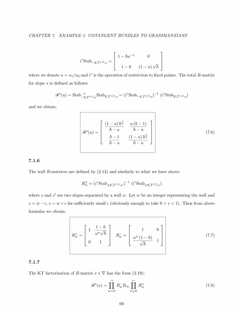
CHAPTER 7. EXAMPLE 1: COTANGENT BUNDLES TO GRASSMANNIANS
i∗Stab−C,T 1/2,s =
1− ~u−1 0
1− ~ (1− u)√~
where we denote u = u1/u2 and i
∗ is the operation of restriction to fixed points. The total R-matrix
for slope s is defined as follows:
Rs(u) = Stab−1−C,T 1/2,sStabC,T 1/2,s = (i∗Stab−C,T 1/2,s)
−1 (i∗StabC,T 1/2,s)
and we obtain:
Rs(u) =
(1− u) ~
12
~− uu (~− 1)
~− u~− 1
~− u(1− u) ~
12
~− u
(7.6)
7.1.6
The wall R-matrices are defined by (2.13) and similarly to what we have above:
R±w = (i∗Stab±C,T 1/2,s′)−1 (i∗Stab±C,T 1/2,s)
where s and s′ are two slopes separated by a wall w. Let w be an integer representing the wall and
s = w− ϵ, s = w+ ϵ for sufficiently small ϵ (obviously enough to take 0 < ϵ < 1). Then from above
formulas we obtain:
R+w =
11− ~uw√~
0 1
R−w =
1 0
uw (1− ~)√~
1
(7.7)
7.1.7
The KT factorization of R-matrix s ∈ ∇ has the form (2.19):
Rs(u) =→∏
w<0
R−wR∞
←∏w≥0
R+w (7.8)
69

CHAPTER 7. EXAMPLE 1: COTANGENT BUNDLES TO GRASSMANNIANS
This infinite product is convergent in the topology of power series in u−1. From (7.7) we obtain:
U =
←∏w≥0
R+w = · · ·R+
1 R+0 =
11− ~√
~(1 + u−1 + · · · )
0 1
=
1(1− ~)u√~ (u− 1)
0 1
L =
→∏w<0
R−w = R−−1R−−2 · · · =
1 0
(1− ~)√~
(u−1 + · · · ) 1
=
1 0
(1− ~)√~ (u− 1)
1
Finally, the infinity slope R-matrix is given by (2.24). The attracting and repealing directions are
obvious from Fig. 7.1 and we obtain:
R∞ = −
u−
12 − u
12
u12~−
12 − u−
12~
12
0
0u−
12~−
12 − u
12~
12
u12 − u−
12
One easily checks that in agreement with (7.6) we have Rs(u) = LR∞ U . This gives canonical
Gauss decomposition of the R-matrix.
7.1.8
The R-matrix for the whole Nakajima variety X given by (7.2) is of the form:
Rs(u) =
1
RsT ∗P
1
=
1 0 0 0
0(1− u)~
12
~− uu(~− 1)
~− u0
0~− 1
~− u(1− u)~
12
~− u0
0 0 0 1
Up to a scalar multiple one recognizes the standard R-matrix for U~(gl2) acting in the tensor
product of two fundamental evaluation modules C2(u1) ⊗ C2(u2). We conclude, that the quiver
algebra corresponding to cotangent bundles to Grassmannians is U~(gQ) = U~(gl2).
7.1.9
The codimension function (2.27) for X is given, obviously, by the following diagonal matrix:
~Ω = diag(1, ~12 , ~
12 , 1)
70

CHAPTER 7. EXAMPLE 1: COTANGENT BUNDLES TO GRASSMANNIANS
We obtain that the wall R-matrices defined by the Theorem 2 have the following explicit form:
R+w =
1 0 0 0
0 ~12 (1− ~)u−w 0
0 0 ~12 0
0 0 0 1
In particular all wall R-matrices are conjugated to the zeroth one by line bundle:
R+w = O(w)R+
0 O(w)−1 (7.9)
with O(w) = diag(1, uw2 , uw1 , 1). One recognizes, that up to a multiple R+
0 coincides with the
standard R-matrix for U~(sl2) in the tensor product of two fundamental representations. Thus,
the wall subalgebra, which is build by FRT procedure from this R-matrix is U~(g0) ≃ U~(sl2). As
the R-matrices for other wall conjugated, we conclude that U~(gw) ≃ U~(sl2) for arbitrary wall w.
7.1.10
To summarize, we have an algebra U~(gQ) = U~(gl2) and a set of subalgebras U~(gw) ≃ U~(sl2)
indexed by walls w ∈ Z. It is convenient to organize this information as follows: let E, F and
K be the standard generators of U~(sl2) which we understand as U~(g0). Then by (7.9) the wall
subalgebra U~(gw) is generated by Ew, Fw and K:
Ew = O(w)EO(w)−1, Fw = O(w)FO(w)−1. (7.10)
Let us denote x+(w) = Ew, x−(w) = F−w. One can check that the relations among these
generators can be summarized as the Drinfeld’s realization of U~(gl2): the algebra U~(gl2) is an
associative algebra with 1 generated over C(~) by the elements x±(k), a(l),K±1 (k ∈ Z, l ∈ Z\0)
71

CHAPTER 7. EXAMPLE 1: COTANGENT BUNDLES TO GRASSMANNIANS
with the following relations:
KK−1 = K−1K = 1
[a(k), a(m)] = 0, [a(k),K±] = 0
Kx±(k)K−1 = ~±2x±(k)
[x+(k), x−(l)] =1
~− ~−1(ψ(k + l)− φ(k + l)
)
[a(k), x±(l)] = ±[2k]~k
x±(l + k)
(7.11)
with∞∑
m=0ψ(m)z−m = K exp
((~− ~−1)
∞∑k=1
a(k)z−k)
∞∑m=0
φ(−m)zm = K−1 exp
(−(~− ~−1)
∞∑k=1
a(−k)z−k)
It may be convenient to visualize U~(gl2) and its subalgebras as in the Figure 7.2 : the wall
U~(gw) corresponds to a line with integer slope w.
a(−2)
a(−1)H
a(1)
a(2)
E−2
E−1E0
E1
E2
F2
F1F0
F−1
F−2
Figure 7.2: The structure of U~(gl2). The line through zero corresponds to slope 2 subalgebra
Uq(sl2) ⊂ U~(gl2) generated by E2, F2,K.
72

CHAPTER 7. EXAMPLE 1: COTANGENT BUNDLES TO GRASSMANNIANS
7.2 R -matrices
7.2.1
To write the formulas for R-matrices for general variety (7.3) it is enough to substitute all formulas
from the previous section by their “universal” versions.
The universal R-matrix for U~(sl2) is well known:
R = ~−H⊗H/2∞∑k=0
(−1)k(~− ~−1)k~−k(k−1)/2
[k]~!F k ⊗ Ek (7.12)
with H related to K as K = ~H . Up to a scalar multiple the codimension function is given
by ~Ω = ~−H⊗H/2 thus, we conclude that there is the following universal formula for the wall
R-matrices:
R+w =
∞∑k=0
(−1)k(~− ~−1)k~−k(k−1)/2
[k]~!F kw ⊗ Ek
w, (7.13)
The lower triangular wall R-matrix is obtained by transposition R−w = (R+w)21.
7.2.2
The KT factorization (2.19) provides the following universal formula for the total R-matrix:
Rs(u) =→∏
w<s
R−w R∞
←∏w≥s
R+w (7.14)
with R±w with given explicitly by (7.13). The R -matrix R∞ is the operator of multiplication by
the class of normal bundles (2.24). It can be conveniently expressed in terms of generators a(m)
corresponding to the infinite slope in the Fig7.2:
R∞ = c ~H⊗H/2 exp((~− ~−1)
∞∑n=1
m
[2m]~a(−n)⊗ a(n)
)where c is some scalar multiple depending on normalization.
73

CHAPTER 7. EXAMPLE 1: COTANGENT BUNDLES TO GRASSMANNIANS
7.3 The quantum difference operator ML (z)
7.3.1
By definition the function ~λ on K-theory of M (1) = M (1, 1)⨿
M (0, 1) as:
~λ =
z on M (1, 1)
1 on M (0, 1)⇔ ~λ =
z 0
0 1
= z12 zH/2
From this and (7.13) we see that the the ABRR equation for U~(sl2) takes the following form:
J+(z)z−H⊗1/2 R = z−H⊗1/2 ~−H⊗H/2J+(z)
with R given by (7.12). This is an equation for strictly upper triangular operator J(z), which means
that:
J+(z) = 1 +∞∑k=1
J+k (z)F k ⊗Ek
The Proposition 5 says that ABRR equation determines the coefficients Jk(z) uniquely. Computa-
tion gives:
J+(z) =
∞∑k=0
(−1)k~−k(k−1)/2(~− ~−1)k
[k]~!k∏
i=1(1− z−1K ⊗K−1~2i)
F k ⊗ Ek
7.3.2
By definition (5.7) we have J+w(λ) = J+
w (λ − τw). In out case τw = w and this corresponds to a
shift z → z~−sw = zq−w for integer wall w. We conclude that:
J+w(z) =
∞∑k=0
(−1)k~−k(k−1)/2(~− ~−1)k
[k]~!k∏
i=1(1− z−1qwK ⊗K−1~2i)
F kw ⊗ Ek
w (7.15)
7.3.3
The operator Bw(z) is given by (5.9). To compute it, we need the formulas for antipode Sw of
U~(gw). They can be obtained directly form the wallR-matrix (7.13). First, from 1⊗∆(R) = R13R12
and ∆⊗ 1(R) = R13R23 we obtain:
∆(E) = K−1 ⊗ E + E ⊗ 1, ∆(F ) = 1⊗ F + F ⊗K, ∆(K) = K ⊗K
and thus the antipode corresponding to this coproduct has the form:
S(E) = −KE, S(F ) = −FK−1, S(K) = K−1
74
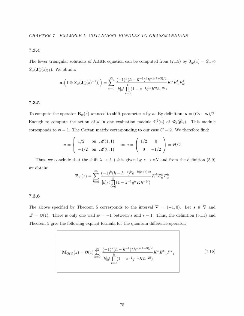
CHAPTER 7. EXAMPLE 1: COTANGENT BUNDLES TO GRASSMANNIANS
7.3.4
The lower triangular solutions of ABRR equation can be computed from (7.15) by J−w(z) = Sw ⊗
Sw(J+w(z)21). We obtain:
m(1⊗ Sw(J−w(z)−1))
)=
∞∑k=0
(−1)k(~− ~−1)k~−k(k+3)/2
[k]~!k∏
i=0(1− z−1qwK2~−2i)
KkEkwF
kw
7.3.5
To compute the operator Bw(z) we need to shift parameter z by κ. By definition, κ = (Cv−w)/2.
Enough to compute the action of κ in one evaluation module C2(u) of U~(gl2). This module
corresponds to w = 1. The Cartan matrix corresponding to our case C = 2. We therefore find:
κ =
1/2 on M (1, 1)
−1/2 on M (0, 1)⇔ κ =
1/2 0
0 −1/2
= H/2
Thus, we conclude that the shift λ → λ + κ is given by z → zK and from the definition (5.9)
we obtain:
Bw(z) =
∞∑k=0
(−1)k(~− ~−1)k~−k(k+3)/2
[k]~!k∏
i=0(1− z−1qwK~−2i)
KkEkwF
kw
7.3.6
The alcove specified by Theorem 5 corresponds to the interval ∇ = (−1, 0). Let s ∈ ∇ and
L = O(1). There is only one wall w = −1 between s and s − 1. Thus, the definition (5.11) and
Theorem 5 give the following explicit formula for the quantum difference operator:
MO(1)(z) = O(1)∞∑k=0
(−1)k(~− ~−1)k~−k(k+3)/2
[k]~!k∏
i=0(1− z−1q−1K~−2i)
KkEk−1F
k−1
(7.16)
75

CHAPTER 7. EXAMPLE 1: COTANGENT BUNDLES TO GRASSMANNIANS
7.3.7
Using (5.11) we can also rewrite this operator as:
MO(1)(z) =( ∞∑
k=0
(−1)k(~− ~−1)k~−k(k+3)/2
[k]~!k∏
i=0(1− z−1q−1K~−2i)
KkEkF k)O(1).
This form is particularly convenient for explicit computations as it expresses the difference operator
through the standard U~(sl2).
7.3.8
In the limits we obtain:
limz→0
MO(1)(z) = O(1) limq→0
MO(1)(z) = O(1)
Moreover:
limz→∞
MO(1)(zq−1) =
( ∞∑k=0
(−1)k(~− ~−1)k~−k(k+3)/2
[k]~!k∏
i=0(1− z−1K~−2i)
KkEkF k)O(1)
And therefore we can find the explicit form of glueing matrix, which plays an important role in
quantum K-theory [31]:
G =∞∑k=0
(−1)k(~− ~−1)k~−k(k+3)/2
[k]~!k∏
i=0(1− z−1K~−2i)
KkEkF k
7.3.9
The fixed point set T ∗Gr(k, n)A consists of n!/(n − k)!/k! points labeled by k-subsets of the set
1, 2, · · · , n. In the basis of stable envelopes of the fixed points on X = T ∗P1 ordered as [[1], [2]]
the difference operator takes the following explicit form:
MO(1)(z/q) =
(z − 1)u1
z~2 − 1
z(~− ~−1
)u2
(1− z~2)(~− ~−1
)u1
(1− z~2)(z − 1)u2z~2 − 1
76
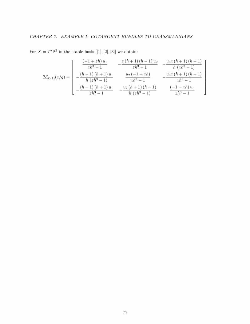
CHAPTER 7. EXAMPLE 1: COTANGENT BUNDLES TO GRASSMANNIANS
For X = T ∗P2 in the stable basis [[1], [2], [3]] we obtain:
MO(1)(z/q) =
(−1 + z~)u1z~3 − 1
−z (~+ 1) (~− 1)u2z~3 − 1
−u3z (~+ 1) (~− 1)
~ (z~3 − 1)
−(~− 1) (~+ 1)u1~ (z~3 − 1)
u2 (−1 + z~)z~3 − 1
−u3z (~+ 1) (~− 1)
z~3 − 1
−(~− 1) (~+ 1)u1z~3 − 1
−u2 (~+ 1) (~− 1)
~ (z~3 − 1)
(−1 + z~)u3z~3 − 1
77
CHAPTER 8. EXAMPLE 2: INSTANTON MODULI SPACES
Chapter 8
Example 2: Instanton moduli spaces
In this section we consider the example of Jordan quiver: the quiver consisting of one vertex and
a single loop. The dimension vectors are given by two non-negative integer numbers v = n, w = r.
The corresponding variety M (n, r) is the moduli space of framed rank r torsion-free sheaves F on
P2 with fixed second Chern class c2(F) = n. A framing of a sheaf F is a choice of of an isomorphism:
ϕ : F|L∞ → O⊕rL∞(8.1)
where L∞ is the line at infinity of C2 ⊂ P2. This moduli space is usually referred to as instanton
moduli space.
Let A ≃ (C×)r be the framing torus acting on M (n, r) by changing the isomorphism (8.1). This
torus acts on the instanton moduli space preserving the symplectic form.
Let us denote by G = A × (C×)2 where the second factor acts on C2 ⊂ P2 by scaling the
coordinates. This induces an action of G on M (n, r). The action of this torus scales the symplectic
form with a character which we denote by ~.
We denote the equivariant parameters corresponding to A by u1, · · · , ur, and to torus G/A by
t1, t2 such that the weight of the symplectic form is:
~ = t1t2
78
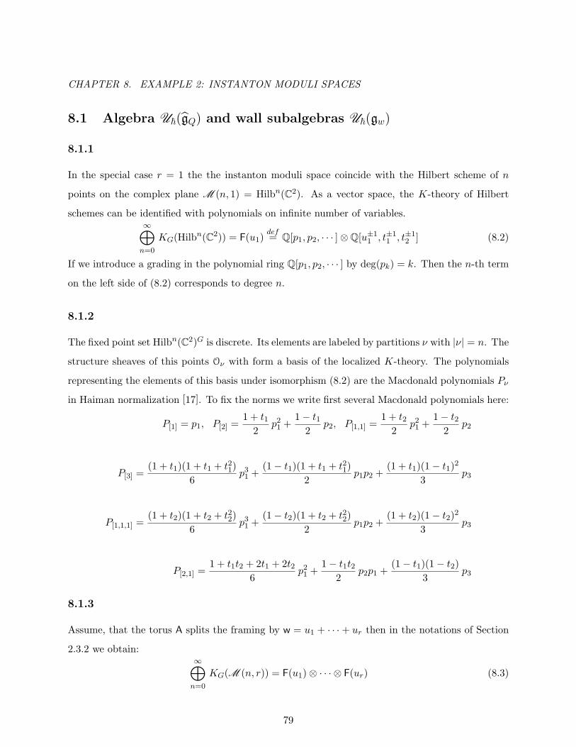
CHAPTER 8. EXAMPLE 2: INSTANTON MODULI SPACES
8.1 Algebra U~(gQ) and wall subalgebras U~(gw)
8.1.1
In the special case r = 1 the the instanton moduli space coincide with the Hilbert scheme of n
points on the complex plane M (n, 1) = Hilbn(C2). As a vector space, the K-theory of Hilbert
schemes can be identified with polynomials on infinite number of variables.∞⊕n=0
KG(Hilbn(C2)) = F(u1)def= Q[p1, p2, · · · ]⊗Q[u±11 , t±11 , t±12 ] (8.2)
If we introduce a grading in the polynomial ring Q[p1, p2, · · · ] by deg(pk) = k. Then the n-th term
on the left side of (8.2) corresponds to degree n.
8.1.2
The fixed point set Hilbn(C2)G is discrete. Its elements are labeled by partitions ν with |ν| = n. The
structure sheaves of this points Oν with form a basis of the localized K-theory. The polynomials
representing the elements of this basis under isomorphism (8.2) are the Macdonald polynomials Pν
in Haiman normalization [17]. To fix the norms we write first several Macdonald polynomials here:
P[1] = p1, P[2] =1 + t1
2p21 +
1− t12
p2, P[1,1] =1 + t2
2p21 +
1− t22
p2
P[3] =(1 + t1)(1 + t1 + t21)
6p31 +
(1− t1)(1 + t1 + t21)
2p1p2 +
(1 + t1)(1− t1)2
3p3
P[1,1,1] =(1 + t2)(1 + t2 + t22)
6p31 +
(1− t2)(1 + t2 + t22)
2p1p2 +
(1 + t2)(1− t2)2
3p3
P[2,1] =1 + t1t2 + 2t1 + 2t2
6p21 +
1− t1t22
p2p1 +(1− t1)(1− t2)
3p3
8.1.3
Assume, that the torus A splits the framing by w = u1 + · · ·+ ur then in the notations of Section
2.3.2 we obtain:∞⊕n=0
KG(M (n, r)) = F(u1)⊗ · · · ⊗ F(ur) (8.3)
79

CHAPTER 8. EXAMPLE 2: INSTANTON MODULI SPACES
8.1.4
Let us set Z = Z2, Z∗ = Z (0, 0) and:
Z+ = (i, j) ∈ Z; i > 0 or i = 0, j > 0, Z− = −Z+
Set
nk =(t
k21 − t
− k2
1 )(tk22 − t
− k2
2 )(~−k2 − ~
k2 )
k
and for vector a = (a1, a2) ∈ Z denote by deg(a) the greatest common divisor of a1 and a2. We set
ϵa = ±1 for a ∈ Z±. For a pair non-collinear vectors we set ϵa,b = sign(det(a,b)).
The “toroidal” algebra Uq(gl1) is an associative algebra with 1 generated by elements ea and
Ka with a ∈ Z, subject to the following relations [37]:
• elements Ka are central and
K0 = 1, KaKb = Ka+b
• if a, b are two collinear vectors then:
[ea, eb] = δa+bK−1a −Ka
ndeg(a)(8.4)
• if a and b are such that deg(a) = 1 and the triangle (0, 0),a,b has no interior lattice points
then
[ea, eb] = ϵa,bKα(a,b)Ψa+b
n1
where
α(a,b) =
ϵa(ϵaa+ ϵbb− ϵa+b(a+ b))/2 if ϵa,b = 1
ϵb(ϵbb+ ϵbb− ϵa+b(a+ b))/2 if ϵa,b = −1
and elements Ψa are defined by:
∞∑k=0
Ψkazk = exp
( ∞∑m=1
nm emazm)
for a ∈ Z such that deg(a) = 1.
It is convenient to visualize the algebra Uq(gl1) as in the Figure 8.1. Heisenberg subalgebras of
Uq(gl1) are labeled by w ∈ Q and correspond to lines with slope w in this picture.
80

CHAPTER 8. EXAMPLE 2: INSTANTON MODULI SPACES
e(2,−2)
e(2,−1)e(2,0)
e(2,1)
e(2,2)
e(0,−2)
e(0,−1)
e(0,1)
e(0,2)
e(1,−2)
e(1,−1)e(1,0)
e(1,1)
e(1,2)
e(−1,−2)
e(−1,−1)e(−1,0)
e(−1,1)
e(−1,2)
e(−2,−2)
e(−2,−1)e(−2,0)
e(−2,1)
e(−2,2)
Figure 8.1: The line with slope 2 corresponds to Heisenberg subalgebra generated by ek,2k for k ∈ Z.
8.1.5
The action of Uq(gl1) on the K-theory (8.2) was constructed in [37]. The central elements act in
this representation by:
K(1,0) = t− 1
21 t
− 12
2 , K(0,1) = 1 (8.5)
In particular, the “vertical” generators commute commute in (8.2):
[e(0,m), e(0,n)] = 0
and “horizontal” form a Heisenberg subalgebra:
[e(m,0), e(n,0)] =−m
(tm/21 − t−m/2
1 )(tm/22 − t−m/2
2 )δn+m
Explicitly, these generators act as follows:
e(m,0) =
1
(tm/21 − t−m/2
1 )(tm/22 − t−m/2
2 )p−m m < 0
−m ∂
∂pmm > 0
(8.6)
and
e(0,m)(Pν) = u−m1 sign(k)
(1
1− tm1
∞∑i=1
tm(λi−1)1 t
m(i−1)2
)Pν (8.7)
81

CHAPTER 8. EXAMPLE 2: INSTANTON MODULI SPACES
It is clear that e(0,m) and e(m,0) generate the whole Uq(gl1). Thus the last two formulas give explicit
presentation of Uq(gl1) action on the Fock space.
8.1.6
The geometric R -matrix for the instanton moduli space was computed in [27]. It was shown that
thisR -matrix coincide withR -matrix for Uq(gl1). In particular, this implies that U~(gQ) ≃ Uq(
gl1).8.2 R-matrices
8.2.1
Recall, that the quantum Heisenberg algebra is an algebra generated by elements e, f and a cental
element K modulo the following relations:
[e, e] = [f, f ] = 0, [e, f ] =K −K−1
c− c−1(8.8)
The Fock space F = Q[x]⊗Q[c±1] is a natural module over the Heisenberg algebra with the following
cation:
e(p) = xp, f(p) = −dpdx, K(p) = cp
so that c is a formal parameter fixing value of cental element K in F. The Heisenberg algebra is a
Hopf algebra with the following coproduct:
∆(e) = e⊗ 1 +K−1 ⊗ e
∆(f) = f ⊗K + 1⊗ f
∆(K) = K ⊗K
antipode:
S(e) = −Ke, S(f) = −K−1f, S(K) = K−1
and counit:
ε(e) = ε(f) = 0, ε(K) = 1
82
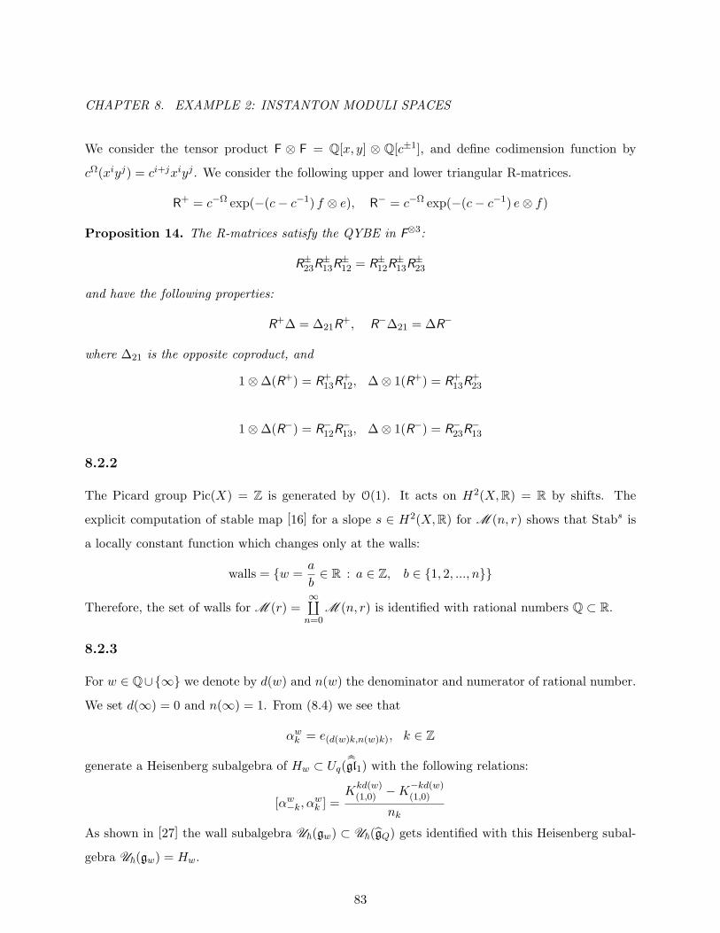
CHAPTER 8. EXAMPLE 2: INSTANTON MODULI SPACES
We consider the tensor product F ⊗ F = Q[x, y] ⊗ Q[c±1], and define codimension function by
cΩ(xiyj) = ci+jxiyj . We consider the following upper and lower triangular R-matrices.
R+ = c−Ω exp(−(c− c−1) f ⊗ e), R− = c−Ω exp(−(c− c−1) e⊗ f)
Proposition 14. The R-matrices satisfy the QYBE in F⊗3:
R±23R±13R±12 = R±12R
±13R±23
and have the following properties:
R+∆ = ∆21R+, R−∆21 = ∆R−
where ∆21 is the opposite coproduct, and
1⊗∆(R+) = R+13R
+12, ∆⊗ 1(R+) = R+
13R+23
1⊗∆(R−) = R−12R−13, ∆⊗ 1(R−) = R−23R
−13
8.2.2
The Picard group Pic(X) = Z is generated by O(1). It acts on H2(X,R) = R by shifts. The
explicit computation of stable map [16] for a slope s ∈ H2(X,R) for M (n, r) shows that Stabs is
a locally constant function which changes only at the walls:
walls = w =a
b∈ R : a ∈ Z, b ∈ 1, 2, ..., n
Therefore, the set of walls for M (r) =∞⨿n=0
M (n, r) is identified with rational numbers Q ⊂ R.
8.2.3
For w ∈ Q∪∞ we denote by d(w) and n(w) the denominator and numerator of rational number.
We set d(∞) = 0 and n(∞) = 1. From (8.4) we see that
αwk = e(d(w)k,n(w)k), k ∈ Z
generate a Heisenberg subalgebra of Hw ⊂ Uq(gl1) with the following relations:
[αw−k, α
wk ] =
Kkd(w)(1,0) −K
−kd(w)(1,0)
nk
As shown in [27] the wall subalgebra U~(gw) ⊂ U~(gQ) gets identified with this Heisenberg subal-
gebra U~(gw) = Hw.
83

CHAPTER 8. EXAMPLE 2: INSTANTON MODULI SPACES
8.2.4
We conclude, that the R-matrix R+w for the wall w ∈ Q corresponding to the Heisenberg subalgebra
U~(gw) takes the form:
R+w =
∞∏k=0
exp(−nk αwk ⊗ αw
−k) = exp(−∞∑k=0
nk αwk ⊗ αw
−k
)The lower triangular R-matrix is obtained by the transposition:
R−w =
∞∏k=0
exp(−nk αw−k ⊗ αw
k ) = exp(−∞∑k=0
nk αw−k ⊗ αw
k
)As the cental element of the elliptic Hall algebra acts in the Fock K-theory by K(1,0) = ~−1/2
cental parameter c of the quantum Heisenber algebra generated by e = αw−k and f = αw
k is given
by c = ~−kd(w)/2 = (t1t2)−kd(w)/2.
8.2.5
Let us fix a slope s ∈ H2(X,R) = R. The Khoroshkin-Tolstoy factorization (2.19) provides the
following universal formula for the total R-matrix:
Rs(u) =→∏
w∈Qw<s
R−w R∞
←∏w∈Qw>s
R+w (8.9)
The infinite slope R -matrix R∞ is the operator of multiplication by normal bundles (2.24). From
explicit formula for action of α∞k (8.7) we can obtain:
R∞ = exp(−∞∑k=0
nk α∞−k ⊗ α∞k
)This, together with formulas from the previous section give the following beautiful universal ex-
pression for a slope s R-matrix:
Rs(u) =←s∏
w∈Q∪∞
exp(−∞∑k=0
nk αw−k ⊗ αw
k
)
8.3 The quantum difference operator ML (z)
8.3.1
Assume that r = 2 such that KG(M (r)A) = F(u1)⊗ F(u2). In this situation
M (n, 2)A =⨿
n1+n2=n
Hilbn1(C2)×Hilbn2(C2)
84
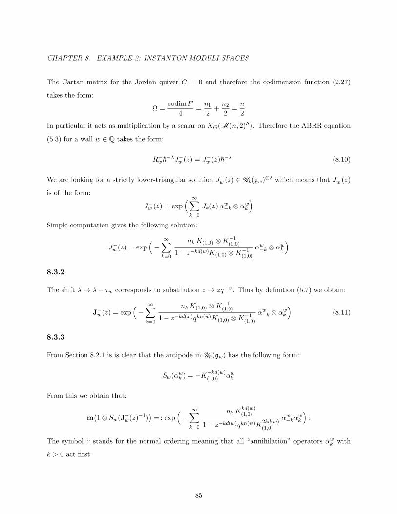
CHAPTER 8. EXAMPLE 2: INSTANTON MODULI SPACES
The Cartan matrix for the Jordan quiver C = 0 and therefore the codimension function (2.27)
takes the form:
Ω =codimF
4=n12
+n22
=n
2
In particular it acts as multiplication by a scalar on KG(M (n, 2)A). Therefore the ABRR equation
(5.3) for a wall w ∈ Q takes the form:
R−w~−λJ−w (z) = J−w (z)~−λ (8.10)
We are looking for a strictly lower-triangular solution J−w (z) ∈ U~(gw)⊗2 which means that J−w (z)
is of the form:
J−w (z) = exp( ∞∑
k=0
Jk(z)αw−k ⊗ αw
k
)Simple computation gives the following solution:
J−w (z) = exp(−∞∑k=0
nkK(1,0) ⊗K−1(1,0)
1− z−kd(w)K(1,0) ⊗K−1(1,0)
αw−k ⊗ αw
k
)8.3.2
The shift λ→ λ− τw corresponds to substitution z → zq−w. Thus by definition (5.7) we obtain:
J−w(z) = exp(−∞∑k=0
nkK(1,0) ⊗K−1(1,0)
1− z−kd(w)qkn(w)K(1,0) ⊗K−1(1,0)
αw−k ⊗ αw
k
)(8.11)
8.3.3
From Section 8.2.1 is is clear that the antipode in U~(gw) has the following form:
Sw(αwk ) = −K
−kd(w)(1,0) αw
k
From this we obtain that:
m(1⊗ Sw(J−w(z)−1)
)= : exp
(−∞∑k=0
nkKkd(w)(1,0)
1− z−kd(w)qkn(w)K2kd(w)(1,0)
αw−kα
wk
):
The symbol :: stands for the normal ordering meaning that all “annihilation” operators αwk with
k > 0 act first.
85

CHAPTER 8. EXAMPLE 2: INSTANTON MODULI SPACES
8.3.4
The Cartan matrix of the Jordan quiver is trivial C = 0 and therefore κ = (Cv − w)/2 = −r/2.
The shift λ→ λ+ κ thus corresponds to z → z~−r/2, of for all r at once z → z K(1,0). From (5.9)
we obtain:
Bw(z) =: exp( ∞∑
k=0
nkKkd(w)(1,0)
1− z−kd(w)qkn(w)Kkd(w)(1,0)
αw−kα
wk
):
8.3.5
Let L = O(1) be the generator of Picard group. Let ∇ ⊂ R be the alcove specified by Theorem 5.
If s ∈ ∇, then the interval (s, s −L ) contains all walls w ∈ Q such that −1 ≤ w < 0. Therefore,
by definition (5.11) we obtain the following explicit formula for quantum difference operator:
MO(1)(z) = O(1)←∏
w∈Q−1≤w<0
: exp( ∞∑
k=0
nk ~−krd(w)/2
1− z−kd(w)qkn(w)~−krd(w)/2αw−kα
wk
): (8.12)
where we used that in the K-theory of instanton moduli space M (n, r) the central element acts by
the scalar K(1,0) = ~−r/2.
8.3.6
Let us consider some limits of the difference operator. First, for all terms in in the previous formula
d(w) > 0 and n(w) < 0. Thus we have:
limq→0
MO(1)(z) = limz→0
MO(1)(z) = O(1)
Second, to compute the limit of MO(1)(zq−1) as q → ∞ we note that for all terms in (8.12)
d(w) + n(w) ≥ 0. Moreover d(w) + n(w) = 0 only for w = −1. We conclude that:
limq→∞
MO(1)(zq−1) = O(1) : exp
( ∞∑k=0
nk ~−kr/2
1− z−k~−kr/2α−1−kα
−1k
):
In the quantum K-theory the glueing matrix can be defined as the limit:
G = limq→∞
ML (zq−1)L −1
86

CHAPTER 8. EXAMPLE 2: INSTANTON MODULI SPACES
for ample L . We note, that O(1)αwk O(1)
−1 = αw+1k , which gives the following formula for G
matrix:
G =: exp( ∞∑
k=0
nk ~−kr/2
1− z−k~−kr/2α0−kα
0k
):
The action of “horizontal” Heisenberg algebra α0k on the K-theory is given by (8.6). Using these
formula gluing matrix can be easily computed explicitly.
8.3.7
Let us consider the example of X = Hilb2(C2). The walls which contribute to (8.12) are w = −1
and w = −1/2. The quantum difference operator takes the form:
AO(1) = T−1z O(1)B−1(z)B− 12(z)
Using the identity (6.12) we can also write it in the form:
AO(1) = B0(z)B 12(z)O(1)T−1z
which means that:
MO(1)(zq−1) = B0(z)B 1
2(z)O(1)
We consider the basis of stable envelopes s[1,1] s[2]. This basis in the Fock space is given by the
plethystic Schur polynomials [16].In this basis we obtain explicitly:
B0(z~1/2) =z − 1
(z2t12t22 − 1) (zt1t2 − 1)
z2t1t2 − 1 − (t1t2 − 1) z
− (t1t2 − 1) z z2t1t2 − 1
B 12(z~1/2) = 1 +
z2 (t1t2 − 1)
z2t12t22 − q
−1 t2
t1 −t1t2
O(1) =
t2 0
−t1t2 + 1 t1
87

CHAPTER 8. EXAMPLE 2: INSTANTON MODULI SPACES
8.3.8
Let us consider the example of X = Hilb2(C3). Similarly, in this case the quantum difference
operator takes the form:
MO(1)(zq−1) = B0(z)B 1
3(z)B 1
2(z)B 2
3(z)O(1)
In the stable basis ordered as s[1,1,1], s[2,1], s[3] we obtain explicitly:
88

CHAPTER 8. EXAMPLE 2: INSTANTON MODULI SPACES
B0(z~1/2) = (z−1)(zt1t2+1)(t1t2−1)(z3t13t23−1)(z2t12t22−1)(zt1t2−1)×
(z2t1t2−1)(z3t12t22−1)
(t1t2−1)(zt1t2+1) −z(z2t1t2 − 1
) z2(zt12t22−1)zt1t2+1
−z(z2t1t2 − 1
)z4t12t22−z3t12t22+z2t12t22−2 z2t1t2+z2−z+1
t1t2−1 −z(z2t1t2 − 1
)z2(zt12t22−1)
zt1t2+1 −z(z2t1t2 − 1
) (z2t1t2−1)(z3t12t22−1)(t1t2−1)(zt1t2+1)
B1/3(z~1/2) = 1 + z3(t1t2−1)z3t13t23−q
−1 t2 −t22
t1 −t1t2 t1t22
−t12 t12t2 −t22t12
B1/2(z~1/2) = 1 + z2t1t2(t1t2−1)z2t12t22−q ×
− t1t2+t1−1
t12t2t1t2−1t12
t2t12
(t1t2−1)(t1t2+t1−1)t22t12
− (t1t2−1)2t12t2
− t1t2−1t12
− (t1t2+t1−1)(t1t2−t1−1)t1t22
(t1t2−1)(t1t2−t1−1)t1t2
t1t2−t1−1t1
B2/3(z~1/2) = 1 + z3(t1t2−1)t1t2z3t13t23−q2 ×
t1t22−t1−t2
t12t2− t2(t1t2−t1−1)
t12− t22
t12
− (t1t2+t1−1)(t1t22−t1−t2)t22t12
(t1t2+t1−1)(t1t2−t1−1)t12
t2(t1t2+t1−1)t12
(t12+t1t2−1)(t1t22−t1−t2)t1t22
− (t1t2−t1−1)(t12+t1t2−1)t1
− t2(t12+t1t2−1)t1
O(1) =
t2
3 0 0
− (t1t2 − 1) (t2 + 1) t2 t1t2 0
(t1t2 − 1)(t2t1
2 + t22t1 − 1
)− (t1t2 − 1) (t1 + 1) t1 t1
3
89
CHAPTER 8. EXAMPLE 2: INSTANTON MODULI SPACES
90

BIBLIOGRAPHY
Bibliography
[1] M. Aganagic and A. Okounkov. In preparation.
[2] M. Balagovic. Degeneration of trigonometric dynamical difference equations for quantum loop
algebras to trigonometric Casimir equations for Yangians. Comm. Math. Phys., 334(2):629–
659, 2015.
[3] R. Bezrukavnikov and M. Finkelberg. Wreath Macdonald polynomials and the categorical
McKay correspondence. Camb. J. Math., 2(2):163–190, 2014. With an appendix by Vadim
Vologodsky.
[4] R. Bezrukavnikov and D. Kaledin. Fedosov quantization in positive characteristic. J. Amer.
Math. Soc., 21(2):409–438, 2008.
[5] R. Bezrukavnikov and I. Losev. Etingof conjecture for quantized quiver varieties. 2013.
[6] R. Bezrukavnikov and I. Losev. Etingof conjecture for quantized quiver varieties II. 2014.
[7] R. Bezrukavnikov and I. Mirkovic. Representations of semisimple Lie algebras in prime char-
acteristic and the noncommutative Springer resolution. Ann. of Math. (2), 178(3):835–919,
2013.
[8] R. Bezrukavnikov and A. Okounkov. In preparation.
[9] D. A. Cox and S. Katz. Mirror symmetry and algebraic geometry, volume 68 of Mathematical
Surveys and Monographs. American Mathematical Society, Providence, RI, 1999.
[10] P. Etingof. Symplectic reflection algebras and affine Lie algebras. Mosc. Math. J., 12(3):543–
565, 668–669, 2012.
91

BIBLIOGRAPHY
[11] P. Etingof, T. Schedler, and O. Schiffmann. Explicit quantization of dynamical r-matrices for
finite dimensional semisimple Lie algebras. J. Amer. Math. Soc., 13(3):595–609 (electronic),
2000.
[12] P. Etingof and A. Varchenko. Exchange dynamical quantum groups. Comm. Math. Phys.,
205(1):19–52, 1999.
[13] P. Etingof and A. Varchenko. Dynamical Weyl groups and applications. Adv. Math., 167(1):74–
127, 2002.
[14] I. B. Frenkel and N. Yu. Reshetikhin. Quantum affine algebras and holonomic difference
equations. Commun. Math. Phys., 146:1–60, 1992.
[15] A. Givental. A tutorial on quantum cohomology. In Symplectic geometry and topology (Park
City, UT, 1997), volume 7 of IAS/Park City Math. Ser., pages 231–264. Amer. Math. Soc.,
Providence, RI, 1999.
[16] E. Gorsky and A. Negut. Refined knot invariants and Hilbert schemes. J. Math. Pures Appl.
(9), 104(3):403–435, 2015.
[17] M. Haiman. Notes on Macdonald polynomials and the geometry of Hilbert schemes. In
Symmetric functions 2001: surveys of developments and perspectives, volume 74 of NATO Sci.
Ser. II Math. Phys. Chem., pages 1–64. Kluwer Acad. Publ., Dordrecht, 2002.
[18] D. Kaledin. Derived equivalences by quantization. Geom. Funct. Anal., 17(6):1968–2004, 2008.
[19] S. M. Khoroshkin and V. N. Tolstoy. Universal R-matrix for quantized (super)algebras. Comm.
Math. Phys., 141(3):599–617, 1991.
[20] D. Maulik, N. Nekrasov, A. Okounkov, and R. Pandharipande. Gromov-Witten theory and
Donaldson-Thomas theory. I. Compos. Math., 142(5):1263–1285, 2006.
[21] D. Maulik, N. Nekrasov, A. Okounkov, and R. Pandharipande. Gromov-Witten theory and
Donaldson-Thomas theory. II. Compos. Math., 142(5):1286–1304, 2006.
[22] D. Maulik and A. Oblomkov. Quantum cohomology of the Hilbert scheme of points on An-
resolutions. J. Amer. Math. Soc., 22(4):1055–1091, 2009.
92

BIBLIOGRAPHY
[23] D. Maulik, A. Oblomkov, A. Okounkov, and R. Pandharipande. Gromov-Witten/Donaldson-
Thomas correspondence for toric 3-folds. Invent. Math., 186(2):435–479, 2011.
[24] D. Maulik and A. Okounkov. In preparation.
[25] D. Maulik and A. Okounkov. Quantum Groups and Quantum Cohomology. 2012.
[26] H. Nakajima. Quiver varieties and Kac-Moody algebras. Duke Math. J., 91(3):515–560, 1998.
[27] A. Negut. Quantum Algebras and Cyclic Quiver Varieties. ProQuest LLC, Ann Arbor, MI,
2015. Thesis (Ph.D.)–Columbia University.
[28] N. Nekrasov and A. Okounkov. Membranes and Sheaves. 2014.
[29] N. A. Nekrasov and S. L. Shatashvili. Quantum integrability and supersymmetric vacua. Prog.
Theor. Phys. Suppl., 177:105–119, 2009.
[30] N. A. Nekrasov and S. L. Shatashvili. Supersymmetric vacua and Bethe ansatz. Nuclear Phys.
B Proc. Suppl., 192/193:91–112, 2009.
[31] A. Okounkov. Park City lectures on K-theoretic computations in enumerative geometry. 2015.
[32] A. Okounkov and R. Pandharipande. The quantum differential equation of the Hilbert scheme
of points in the plane. Transform. Groups, 15(4):965–982, 2010.
[33] A. Okounkov and A. Smirnov. Quantum difference equation for Nakajima varieties. 2016.
[34] R. Pandharipande and A. Pixton. Gromov-Witten/Pairs correspondence for the quintic 3-fold.
2012.
[35] N. Y. Reshetikhin. Quasitriangular Hopf algebras and invariants of links. Algebra i Analiz,
1(2):169–188, 1989.
[36] N. Y. Reshetikhin, L. A. Takhtadzhyan, and L. D. Faddeev. Quantization of Lie groups and
Lie algebras. Algebra i Analiz, 1(1):178–206, 1989.
[37] O. Schiffmann and E. Vasserot. The elliptic Hall algebra and the K-theory of the Hilbert
scheme of A2. Duke Math. J., 162(2):279–366, 2013.
93

BIBLIOGRAPHY
[38] V. Tarasov and A. Varchenko. Difference equations compatible with trigonometric KZ differ-
ential equations. Internat. Math. Res. Notices, (15):801–829, 2000.
[39] V. Toledano Laredo. The trigonometric Casimir connection of a simple Lie algebra. J. Algebra,
329:286–327, 2011.
94