Quantum Thermal Bath for Path Integral Molecular DynamicsSimulationFabien Brieuc,† Hichem Dammak,*,†,‡ and Marc Hayoun‡

†Laboratoire Structures, Proprietes et Modelisation des Solides, CentraleSupelec, CNRS, Universite Paris-Saclay, F-92295Chatenay-Malabry, France‡Laboratoire des Solides Irradies, Ecole Polytechnique, CNRS, CEA, Universite Paris-Saclay, F-91128 Palaiseau, France

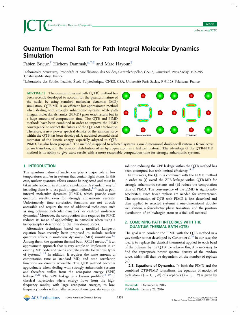
ABSTRACT: The quantum thermal bath (QTB) method hasbeen recently developed to account for the quantum nature ofthe nuclei by using standard molecular dynamics (MD)simulation. QTB-MD is an efficient but approximate methodwhen dealing with strongly anharmonic systems, while pathintegral molecular dynamics (PIMD) gives exact results but ina huge amount of computation time. The QTB and PIMDmethods have been combined in order to improve the PIMDconvergence or correct the failures of the QTB-MD technique.Therefore, a new power spectral density of the random forcewithin the QTB has been developed. A modified centroid-virialestimator of the kinetic energy, especially adapted to QTB-PIMD, has also been proposed. The method is applied to selected systems: a one-dimensional double-well system, a ferroelectricphase transition, and the position distribution of an hydrogen atom in a fuel cell material. The advantage of the QTB-PIMDmethod is its ability to give exact results with a more reasonable computation time for strongly anharmonic systems.

1. INTRODUCTION

The quantum nature of nuclei can play a major role at lowtemperatures and/or in systems that contain light atoms. In thiscase, nuclear quantum effects cannot be neglected and must betaken into account in atomistic simulations. A standard way ofincluding them is to use path integral methods,1−3 such as pathintegral molecular dynamics (PIMD), which provide exactquantum results, even for strongly anharmonic systems.Unfortunately, time correlation functions are not directlyaccessible and require the use of additional techniques suchas ring polymer molecular dynamics4 or centroid moleculardynamics.5 Moreover, the computation time required for PIMDreduces its range of applicability, in particular when using afirst-principles description of the interatomic forces.Alternative techniques based on a modified Langevin

equation have recently been proposed to include nuclearquantum effects in molecular dynamics (MD) simulations.6,7

Among them, the quantum thermal bath (QTB) method6 is anapproximate approach that is very simple to implement in anexisting MD code and yields accurate results for various typesof systems.8−13 In addition, it requires the same amount ofcomputation time as standard MD, and time correlationfunctions are directly accessible. The QTB method becomesapproximate when dealing with strongly anharmonic systemsand therefore suffers from the zero-point energy (ZPE)leakage.14,15 The ZPE leakage is a known problem16−19 inclassical trajectories where energy flows from the high-frequency modes, with large zero-point energies, to low-frequency modes with smaller zero-point energies. An empirical

solution reducing the ZPE leakage within the QTB method hasbeen attempted but with limited efficiency.14,15

In this work, the QTB is combined with the PIMD methodin order to (i) avoid the ZPE leakage within QTB-MD forstrongly anharmonic systems and (ii) reduce the computationtime of PIMD. The convergence of the PIMD is significantlyaccelerated, since fewer replicas are needed for convergence.The combination of QTB with PIMD is first described andthen applied to selected systems: a one-dimensional double-well system, a ferroelectric phase transition, and the positiondistribution of an hydrogen atom in a fuel cell material.

2. COMBINING PATH INTEGRALS WITH THEQUANTUM THERMAL BATH (QTB)

The goal is to combine the PIMD with the QTB method in away similar to that developed by Ceriotti et al.20 In our case, theidea is to replace the classical thermostat applied to each beadof the polymer by the QTB. To achieve this, it is necessary tofind the appropriate power spectral density of the randomforce, which will then be dependent on the number of replicas(P).

2.1. Equations of Dynamics. In both the PIMD and thecombined QTB-PIMD formalisms, the equation of motion ofeach atom i (i = 1, ..., N) of a replica s (s = 1, ..., P) is given by

Received: December 4, 2015Published: January 22, 2016

Article

pubs.acs.org/JCTC

© 2016 American Chemical Society 1351 DOI: 10.1021/acs.jctc.5b01146J. Chem. Theory Comput. 2016, 12, 1351−1359

ω γ = − − − − ++ −⎜ ⎟⎛⎝

⎞⎠P

mp f r r r p R1

(2 )i s i s i P i s i s i s i s i s, ,2

, , 1 , 1 , ,

(1)

where ri,s, pi,s, and fi,s are the atomic position, the momentum,and the force exerted by all the other atoms of the replica s. Thespring constant between beads is equal to

ω =ℏ

mm Pk T

i Pi2 B

2 2

2 (2)

The last two terms of eq 1 correspond to the friction andstochastic forces of the thermostat, respectively.The power spectral density of the random force (IRi

) isobtained from the fluctuation−dissipation theorem:21,22

ω γκ ω=I T m T( , ) 2 ( , )R ii (3)

In standard PIMD, when the Langevin thermostat is used,the stochastic force is a white noise and κ(ω, T) = kB T. For thecombined QTB-PIMD, the power spectral density is ω-dependent and corresponds to the energy of the oscillator ω,which matches the energy θ(ω, T) of the quantum harmonicoscillator when P = 1. κ(ω, T) will be determined in section 2.2.The correlation function of the random force satisfies theWiener−Khinchin theorem:

∫τ ω ωτ ωπ

⟨ + ⟩ = −α α−∞

+∞R t R t I T i( ) ( ) ( , ) exp[ ]

d2i s i s R, , , , i

(4)

The random force Ri,s,α(t) is computed using the numericaltechnique described in the Appendix of ref 23.2.2. Derivation of the Power Spectral Density.

Considering a one-dimensional (1D) harmonic potentialenergy: ω=V x m x( ) 1

22 2, the quantum mean square fluctuation

of the position x at temperature T is given by

ωθ ω

ωβ ω⟨ ⟩ = = ℏ ℏ⎜ ⎟ ⎜ ⎟

⎛⎝

⎞⎠

⎡⎣⎢

⎛⎝

⎞⎠⎤⎦⎥x

mT

m1

( , )2

coth2

22 (5)

where β = 1/(kBT). In the PIMD scheme, one can transformthe coordinates of the P replicas, x1, ..., xs, ..., xP, into normalmodes, q0, ..., qk, ..., qP−1 with pulsations

ω ω ω π= + ⎜ ⎟⎛⎝

⎞⎠P

kP

4 sink P2

22 2

(6)

and the mean square fluctuation is then obtained according to

∑⟨ ⟩ = ⟨ ⟩=

−

xP

q1

k

P

k2

0

12

(7)

The mean potential energy of the normal modes is equal toκ(ωk,T)/2 and then

ωκ ω⟨ ⟩ =

⎛⎝⎜

⎞⎠⎟q

mT

1( , )k

kk

22

(8)

Now, let us determine κ when performing QTB-PIMD. Thefunction κ(ω,T) must allow one to recover the expectedposition fluctuation, which is given by eq 5:

∑ω

κ ωω

β ω= ℏ ℏ

=

−⎜ ⎟

⎡⎣⎢

⎛⎝

⎞⎠⎤⎦⎥P m

Tm

1 1( , )

2coth

2k

P

kk

0

1

2(9)

Defining the dimensionless quantities

β ω= ℏ⎜ ⎟⎛⎝

⎞⎠u

2 (10)

=h u u u( ) coth( ) (11)

β κβ

=ℏ

⎜ ⎟⎛⎝

⎞⎠

⎛⎝⎜

⎞⎠⎟f u

Pu

( )2

P(0)

(12)

eq 9 becomes

∑ ==

− uu

f u h u( ) ( )k

P

kP k

0

1 2

2(0)

(13)

where uk is the reduced pulsation, according to eqs 6 and 10:

π= + ⎜ ⎟⎛⎝

⎞⎠u

uP

PkP

sink2

22

(14)

In the definition of κ, using eq 9, all the normal modes aretreated in the same way. There is an alternative definition24 inwhich the normal mode at k = 0 (centroid of the ring polymer)is classically considered, i.e., κ(ω0, T) = kBT. In this case, eq 9becomes

∑ω ω

κ ωω

β ω+ = ℏ ℏ

=

−⎜ ⎟

⎛⎝⎜

⎞⎠⎟

⎡⎣⎢

⎛⎝

⎞⎠⎤⎦⎥P

k Tm P m

Tm

1 1 1( , )

2coth

2k

P

kk

B

02

1

1

2

(15)

Using the same dimensionless quantities, eq 15 leads to a newequation to be solved:

∑ = −=

− uu

f u h u( ) ( ) 1k

P

kP k

1

1 2

2(1)

(16)

Equations 13 and 16 can be solved by using the self-consistentiterative technique of Ceriotti et al.20 The numerical calculationof f P

(0)25 and f P(1) are reported in the Appendix.

2.3. Estimation of the Macroscopic Properties. In thePIMD method, the potential energy (U) is calculated using theexpression

∑=UP

V r r1

( , ..., )s

s N s1, ,(17)

whereas two expressions for the estimator of the kinetic energyare usually used; the primitive estimator, which is given by

∑ ∑ ω= − − +Km

mp

r r2

12

( )i s

i s

i i si P i s i sprim

,

,2

,

2, , 1

2

(18)

and the centroid-virial estimator, which is given by

∑= − − ·⎜ ⎟⎛⎝

⎞⎠K

Nk T

Pr r f

32

12

( )i s

i s ic

i sCvir B,

, ,(19)

where ric = ∑s ri,s/P is the centroid of the ring polymer i. The

last estimator is known to exhibit weaker fluctuations, which areinsensitive to P, compared to the primitive estimator for whichfluctuations grow with P.2 Combining the QTB and PIMDmethods includes a part of the quantum fluctuations in themomenta, i.e.,

∑ >m

NPk Tp

23

2i s

i s

i,

,2

B

(20)

Journal of Chemical Theory and Computation Article

DOI: 10.1021/acs.jctc.5b01146J. Chem. Theory Comput. 2016, 12, 1351−1359

1352

Thus, eq 19 underestimates the kinetic energy for the QTB-PIMD method and it is more suitable to replace the classicalenergy, 3

2NkBT, by P multiplied by the kinetic energy of the N

normal modes centroids, as follows:

∑ ∑= − − ·K Pm P

pr r f

( )

21

2( )

i

ic

i i si s i

ci smCvir

2

,, ,

(21)

where pic is the momentum of the centroid i. The factor P takes

into account the factor P1/2 between the centroid coordinateand the normal mode coordinate qi,0 = ∑sri,s/P

1/2 of the ring i.The two expressions described by eqs 19 and 21 are

equivalent for any interatomic potential in the case of theoriginal PIMD, but are equivalent only for harmonic potentialsin the case of QTB-PIMD using the f P

(1) function. In the case ofan anharmonic potential, each centroid i, i.e., the normal modeqi,0, is coupled to the other normal modes of the correspondingpolymer. Consequently, the centroid temperature is differentfrom the thermostat temperature (QTB), since some of thequantum effects are included in the momenta of the internalmodes qi,k>0 of the polymer. On the other hand, only eq 21 maybe used for the QTB-PIMD, using the f P

(0) function, because, inthis case, the dynamics of the centroid also includes quantumeffects.Next, we want to compare the two formulations of the QTB-

PIMD method using either the f P(0) or f P

(1) functions (see eqs 13and 16) and to choose the adequate kinetic energy estimatoramong eqs 18, 19, and 21. For this, let us consider a system forwhich the pressure is zero and, thus, the kinetic and potentialcontributions cancel each other out. This allows one to expressthe kinetic energy using the virial estimator (Kvir),

26,27 from thegeneral expression of the pressure:

∑= + ⟨ · ⟩p KP

r f23

13 i s

i s i s,

, ,(22)

∑= − ·KP

r f1

2 i si s i svir

,, ,

(23)

This estimator is used as a reference to validate the relevance ofthe other estimators. The test is performed on two cases of theMorse potential characterized by the dimensionless parameterλ, which is defined as

λα= ℏ

mD1

22

2 2

(24)

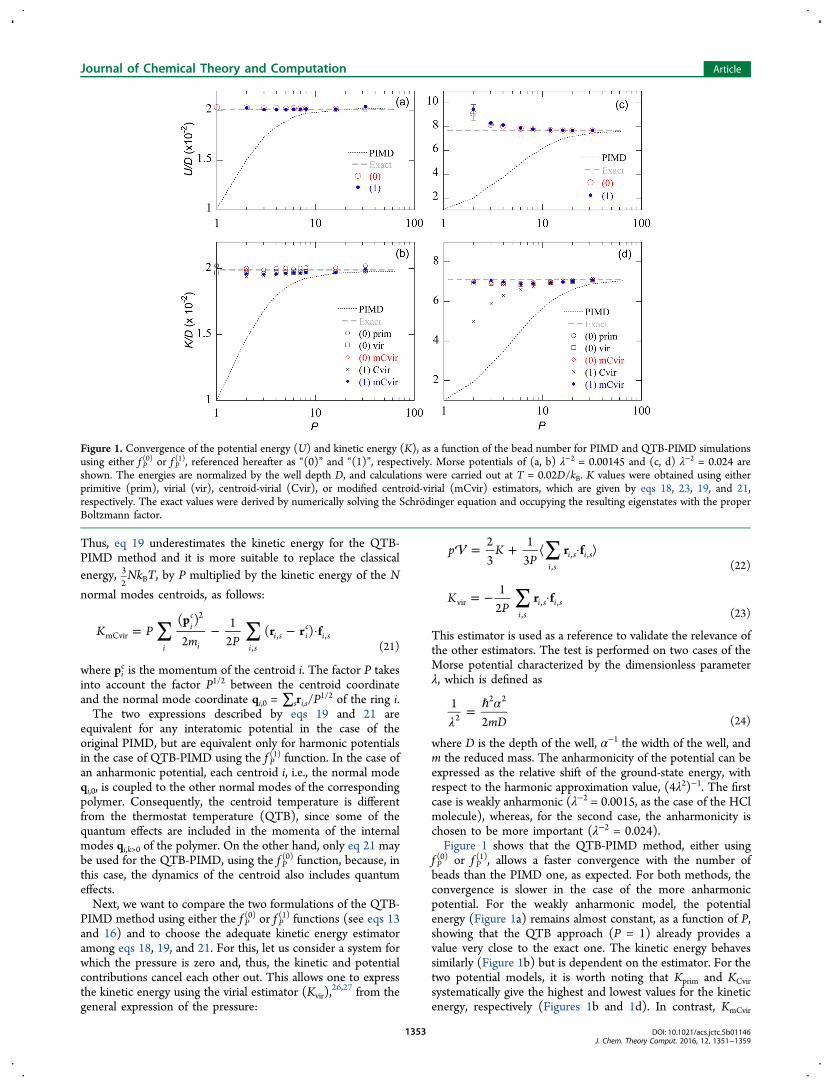
where D is the depth of the well, α−1 the width of the well, andm the reduced mass. The anharmonicity of the potential can beexpressed as the relative shift of the ground-state energy, withrespect to the harmonic approximation value, (4λ2)−1. The firstcase is weakly anharmonic (λ−2 = 0.0015, as the case of the HClmolecule), whereas, for the second case, the anharmonicity ischosen to be more important (λ−2 = 0.024).Figure 1 shows that the QTB-PIMD method, either using

f P(0) or f P

(1), allows a faster convergence with the number ofbeads than the PIMD one, as expected. For both methods, theconvergence is slower in the case of the more anharmonicpotential. For the weakly anharmonic model, the potentialenergy (Figure 1a) remains almost constant, as a function of P,showing that the QTB approach (P = 1) already provides avalue very close to the exact one. The kinetic energy behavessimilarly (Figure 1b) but is dependent on the estimator. For thetwo potential models, it is worth noting that Kprim and KCvirsystematically give the highest and lowest values for the kineticenergy, respectively (Figures 1b and 1d). In contrast, KmCvir

Figure 1. Convergence of the potential energy (U) and kinetic energy (K), as a function of the bead number for PIMD and QTB-PIMD simulationsusing either f P

(0) or f P(1), referenced hereafter as “(0)” and “(1)”, respectively. Morse potentials of (a, b) λ−2 = 0.00145 and (c, d) λ−2 = 0.024 are

shown. The energies are normalized by the well depth D, and calculations were carried out at T = 0.02D/kB. K values were obtained using eitherprimitive (prim), virial (vir), centroid-virial (Cvir), or modified centroid-virial (mCvir) estimators, which are given by eqs 18, 23, 19, and 21,respectively. The exact values were derived by numerically solving the Schrodinger equation and occupying the resulting eigenstates with the properBoltzmann factor.

Journal of Chemical Theory and Computation Article

DOI: 10.1021/acs.jctc.5b01146J. Chem. Theory Comput. 2016, 12, 1351−1359

1353

provides values very close to those obtained with Kvir, which isconsidered as a reference in this example. Figure 2 shows the

influence of the effective friction coefficient (γ) on the kineticenergy estimators. It is clearly shown that KmCvir (eq 21)provides the better estimation and is particularly insensitive to γwhen using the f P

(1) function, whereas the primitive estimatorrequires the use of a low value of γ, leading to an increase in thecomputation time.This example shows that both definitions of the f P functions

(eqs 13 and 16) allow similar convergences of the potential andkinetic energies with the number of beads. The best estimatorfor the kinetic energy is the modified centroid-virial estimationthat is given by eq 21. In the following sections, it is also shownthat position distributions of atoms obtained by using f P

(0) orf P(1) are very close.

3. APPLICATIONS3.1. Position Distribution in a One-Dimensional

Double-Well Potential. Let us consider a particle of massm in a double-well potential:

= −⎜ ⎟⎡⎣⎢⎛⎝

⎞⎠

⎤⎦⎥V x V

xa

( ) 10

2 2

(25)

Using reduced units,

= ϵ =yxa

EV

,0 (26)

for the position and the energy, respectively, the equation forthe stationary wave functions ϕ is written as

ϕ ϕ ϕ− + − = ϵCy

ydd

( 1)2

22 2

(27)

where C is a parameter that is dependent on the barrier height(V0) and the distance between the two wells (2a):

= ℏC

ma V(2 )

2

20 (28)

The numerical resolution of eq 27 shows that there exists acritical value for the parameter, C0 = 0.731778, when the

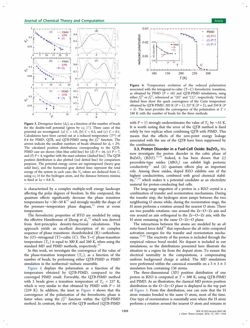
ground-state energy is equal to V0. The eigenvalues rely on C,and we particularly observe that the energy of the ground state(ϵ0) is lower than the height of the energy barrier (i.e., ϵ0 < 1)when C < C0. The motivation behind using such a one-dimensional quartic double-well potential is to provide a simplemodel to check the ability of the QTB-PIMD method torecover the tunnel effect, in contrast to the original QTBapproach.28,29 We investigate the position distribution of aparticle in this double-well potential at a reduced temperatureT* = kBT/ϵ0 = 0.4 for three values of the C parameter: 1, 0.3,and 0.1.The position probability density, ρ(y), which is obtained by

QTB-PIMD simulation, is compared to the exact one, ρ0(y),which is obtained by numerically solving the Schrodingerequation and occupying the resulting eigenstates with theproper Boltzmann factor. The convergence of the density isevaluated by calculating the divergence factor (dP),

∫∫

ρ ρ

ρ=

−−∞

+∞

−∞

+∞dy

y

( ) d

dP

02

02

(29)

which is similar to the reliability factor used in the Rietveldmethod30 to refine a theoretical line profile until it matches anexperimental profile.In all cases, the evolution of the divergence factor and the

distributions as a function of P obtained with the QTB-PIMDmethod are similar when using either the f P

(0) function or thef P(1) function.Figure 3 shows the evolution of the divergence factor as a

function of the number of beads for the three investigatedcases. In the first case, the value of the C parameter (C = 1) isgreater than the critical value C0 (see eq 28) . As shown by thedivergence factor in Figure 3a, the distributions obtained withthe QTB-PIMD and PIMD methods converge to the exact one,within an error of dP ≈ 2% at P = 16 and P = 21, respectively.Hence, the full convergence is especially difficult to reach in thiscase. Indeed, the exact distribution exhibits only one maximum,located at y = 0 (Figure 3d), while a poor convergence leads toa distribution with two maxima. One of these situations isillustrated by the QTB method, which fails dramatically, with anerror of dP = 40%. In the other two cases, C < C0 and all theposition distributions show two maxima (see Figures 3e and3f). For the QTB-PIMD simulation, the number of beadsrequired to converge within an error of dP ≈ 2% decreases as Cdecreases; P = 7 for C = 0.3, and P = 4 for C = 0.1 (see Figures3b and 3c). It is worth noting that, for the lowest value of C, thedistribution obtained with the QTB method is in goodagreement with the exact one. This case corresponds to highvalues of either the barrier height (V0) or the distance betweenthe two wells (2a), or the particle mass (m). In other words, theQTB method succeeds when the tunnel effect is notpredominant.In summary, the combination of the QTB and PIMD

methods allows a better convergence with the number of beads.In fact, for a high accuracy in the position distribution, the gainobtained by QTB-PIMD, with respect to PIMD, is not asimportant and is lower than a factor of 2. In contrast, theadvantage of the QTB-PIMD is more substantiala gain of afactor of 3with respect to the convergence of the totalenergy.

3.2. Ferroelectric−Paraelectric Phase Transition. Wenow investigate the BaTiO3 (BTO) ferroelectric crystal, which

Figure 2. Effect of the effective friction coefficient (γ) on the kineticenergy obtained using the primitive (prim) and modified centroid-virial (mCvir) estimators. “(0)” and “(1)” correspond to QTB-PIMDsimulations using f P

(0) and f P(1) functions, respectively. The relative

deviation from the virial estimator values, (K − Kvir)/Kvir, is plotted. γis normalized by the pulsation ωmin, which is equal to that of thecentroid (normal mode k = 0 of the ring polymer) in the harmonicapproximation: ωmin = ω0 = ω/P1/2 (eq 6). The Morse potential is λ−2

= 0.00145, using P = 4 and T = 0.02D/kB.

Journal of Chemical Theory and Computation Article

DOI: 10.1021/acs.jctc.5b01146J. Chem. Theory Comput. 2016, 12, 1351−1359

1354

is characterized by a complex multiple-well energy landscapeaffecting the polar degrees of freedom. In this compound, thequantum effects significantly decrease the phase transitiontemperatures by ∼30−50 K31 and strongly modify the shape ofthe pressure−temperature phase diagram,32 even at roomtemperature.The ferroelectric properties of BTO are modeled by using

the effective Hamiltonian of Zhong et al.,33 which was derivedfrom first-principles density-functional calculations. Thisapproach yields an excellent description of its complexsequence of phase transitions: rhombohedral (R)−orthorhom-bic (O)−tetragonal (T)−cubic (C). The T−C phase-transitiontemperature (TC) is equal to 300 K and 260 K, when using thestandard MD and PIMD methods, respectively.34

In this work, we investigate the convergence of the value ofthe phase-transition temperature (TC), as a function of thenumber of beads, by performing either QTB-PIMD or PIMDsimulation in the isothermal−isobaric ensemble.Figure 4 displays the polarization as a function of the

temperature obtained by QTB-PIMD, compared to theconverged PIMD result. Favorably, the QTB-PIMD methodwith 2 beads gives a transition temperature of TC = 257 K,which is very similar to that obtained by PIMD with P = 16(259 K). In addition, the inset in Figure 4 shows that theconvergence of the polarization of the ferroelectric phase isfaster when using the f P

(1) function within the QTB-PIMDmethod. In contrast, the use of the QTB method (QTB-PIMD

with P = 1) strongly underestimates the value of TC by ∼55 K.It is worth noting that the error of the QTB method is fixedsolely by two replicas when combining QTB with PIMD. Thismeans that the effects of the zero-point energy leakageassociated with the use of the QTB have been suppressed bythe combination.

3.3. Proton Disorder in a Fuel-Cell Oxide: BaZrO3. Wenow investigate the proton disorder in the cubic phase ofBaZrO3 (BZO).35,36 Indeed, it has been shown that (i)perovskite-type oxides (ABO3) can exhibit high protonicconductivity37 and (ii) quantum effects play an importantrole. Among these oxides, doped BZO exhibits one of thehighest conductivities, combined with good chemical stabil-ity,37,38 which makes it a potential candidate as an electrolytematerial for proton-conducting fuel cells.The long-range migration of a proton in a BZO crystal is a

combination of transfer and reorientation mechanisms. Duringthe transfer step, the hydrogen atom jumps between the twoneighboring O atoms while, during the reorientation stage, theH atom performs a rotation around the nearest O atom. Thereare two possible rotations: one around the Zr−O−Zr axis andone around an axis orthogonal to the Zr−O−Zr axis, with theH atom remaining in the same O−Zr−O plane.The interactions between the atoms are modeled by an ab

initio-based force field39 that reproduces the ab initio computedactivation energies for the transfer and reorientation mecha-nisms.39,40 The reactivity of the proton is included through theempirical valence bond model. No dopant is included in oursimulations, so the distributions presented here illustrate thesituation in a region far from the dopant atom. To ensure theelectrical neutrality in the computations, a compensatinguniform background charge is added. The MD simulationswere performed within the canonical ensemble on a 3 × 3 × 3simulation box containing 136 atoms.The three-dimensional (3D) position distribution of one

proton in BZO is computed at T = 300 K, using QTB-PIMDand PIMD. As an illustration, the classical MD proton positiondistribution in the O−Zr−O plane is displayed in the top partof Figure 5. From this distribution, one can note that the Hatom remains bonded to the same O atom, most of the time.One type of reorientation is essentially seen where the H atomperforms a rotation around the nearest O atom and remains in

Figure 3. Divergence factor (dP), as a function of the number of beadsfor the double-well potential (given by eq 27). Three cases of thispotential are investigated: (a) C = 1.0, (b) C = 0.3, and (c) C = 0.1.Calculations have been carried out at a reduced temperature (T*) of0.4 for PIMD, QTB, and QTB-PIMD using the f P

(1) function. Thearrows indicate the smallest numbers of beads obtained for dP < 2%.The calculated position distributions corresponding to the QTB-PIMD case are shown (thin blue solid line) for (d) P = 16, (e) P = 7,and (f) P = 4, together with the exact solution (dashed line). The QTBposition distribution is also plotted (red dotted line) for comparisonpurposes. The potential energy curves are superimposed (heavy graysolid line), and the horizontal gray dotted lines represent the totalenergy of the system in each case; the V0 values are deduced from C,using eq 28 for the hydrogen atom, and the distance between minimais fixed at 2a = 0.8 Å.

Figure 4. Temperature evolution of the reduced polarizationassociated with the tetragonal-to-cubic (T−C) ferroelectric transition,as obtained by PIMD (P = 16) and QTB-PIMD simulations, usingeither f P

(0) or f P(1), referenced as “(0)” and “(1)”, respectively. Vertical

dashed lines show the quick convergence of the Curie temperatureobtained by QTB-PIMD: 202 K (P = 1), 257 K (P = 2), and 259 K (P= 3). The inset provides the convergence of the polarization at T =240 K with the number of beads for the three methods.

Journal of Chemical Theory and Computation Article

DOI: 10.1021/acs.jctc.5b01146J. Chem. Theory Comput. 2016, 12, 1351−1359

1355

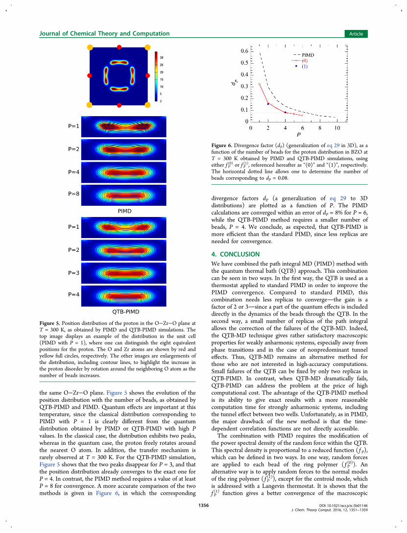
the same O−Zr−O plane. Figure 5 shows the evolution of theposition distribution with the number of beads, as obtained byQTB-PIMD and PIMD. Quantum effects are important at thistemperature, since the classical distribution corresponding toPIMD with P = 1 is clearly different from the quantumdistribution obtained by PIMD or QTB-PIMD with high Pvalues. In the classical case, the distribution exhibits two peaks,whereas in the quantum case, the proton freely rotates aroundthe nearest O atom. In addition, the transfer mechanism israrely observed at T = 300 K. For the QTB-PIMD simulation,Figure 5 shows that the two peaks disappear for P = 3, and thatthe position distribution already converges to the exact one forP = 4. In contrast, the PIMD method requires a value of at leastP = 8 for convergence. A more accurate comparison of the twomethods is given in Figure 6, in which the corresponding

divergence factors dP (a generalization of eq 29 to 3Ddistributions) are plotted as a function of P. The PIMDcalculations are converged within an error of dP = 8% for P = 6,while the QTB-PIMD method requires a smaller number ofbeads, P = 4. We conclude, as expected, that QTB-PIMD ismore efficient than the standard PIMD, since less replicas areneeded for convergence.

4. CONCLUSIONWe have combined the path integral MD (PIMD) method withthe quantum thermal bath (QTB) approach. This combinationcan be seen in two ways. In the first way, the QTB is used as athermostat applied to standard PIMD in order to improve thePIMD convergence. Compared to standard PIMD, thiscombination needs less replicas to convergethe gain is afactor of 2 or 3since a part of the quantum effects is includeddirectly in the dynamics of the beads through the QTB. In thesecond way, a small number of replicas of the path integralallows the correction of the failures of the QTB-MD. Indeed,the QTB-MD technique gives rather satisfactory macroscopicproperties for weakly anharmonic systems, especially away fromphase transitions and in the case of nonpredominant tunneleffects. Thus, QTB-MD remains an alternative method forthose who are not interested in high-accuracy computations.Small failures of the QTB can be fixed by only two replicas inQTB-PIMD. In contrast, when QTB-MD dramatically fails,QTB-PIMD can address the problem at the price of highcomputational cost. The advantage of the QTB-PIMD methodis its ability to give exact results with a more reasonablecomputation time for strongly anharmonic systems, includingthe tunnel effect between two wells. Unfortunately, as in PIMD,the major drawback of the new method is that the time-dependent correlation functions are not directly accessible.The combination with PIMD requires the modification of

the power spectral density of the random force within the QTB.This spectral density is proportional to a reduced function ( f P),which can be defined in two ways. In one way, random forcesare applied to each bead of the ring polymer ( f P

(0)). Analternative way is to apply random forces to the normal modesof the ring polymer ( f P

(1)), except for the centroid mode, whichis addressed with a Langevin thermostat. It is shown that thef P(1) function gives a better convergence of the macroscopic

Figure 5. Position distribution of the proton in the O−Zr−O plane atT = 300 K, as obtained by PIMD and QTB-PIMD simulations. Thetop image displays an example of the distribution in the unit cell(PIMD with P = 1), where one can distinguish the eight equivalentpositions for the proton. The O and Zr atoms are shown by red andyellow full circles, respectively. The other images are enlargements ofthe distribution, including contour lines, to highlight the increase inthe proton disorder by rotation around the neighboring O atom as thenumber of beads increases.

Figure 6. Divergence factor (dP) (generalization of eq 29 in 3D), as afunction of the number of beads for the proton distribution in BZO atT = 300 K obtained by PIMD and QTB-PIMD simulations, usingeither f P

(0) or f P(1), referenced hereafter as “(0)” and “(1)”, respectively.

The horizontal dotted line allows one to determine the number ofbeads corresponding to dP = 0.08.

Journal of Chemical Theory and Computation Article

DOI: 10.1021/acs.jctc.5b01146J. Chem. Theory Comput. 2016, 12, 1351−1359

1356

quantities with the number of beads than f P(0). Considering that

some of the quantum fluctuations are included in the momentathrough the QTB contribution, a modified centroid-virialestimator of the kinetic energy is proposed. This estimator isaccurate and insensitive to the effective friction coefficient whenusing the f P

(1) function.The combination procedure is similar to that presented by

Ceriotti et al.20 The iterative algorithm described in theAppendix to determine the f P function is the same as that usedto establish the gP function of ref 20. The difference lies in thechoice of the thermostat used to include the quantum effects. Inthe colored-noise thermostat (GLE) of Ceriotti et al.,7 thequantum effects are introduced through a dispersive frictioncoefficient, whereas, in the QTB case, the quantum effects areincluded through the power spectral density of the randomforce. The two methods are basically equivalent, but the QTB-MD method is easier to implement in a PIMD code. Knowingthe f P function, the random forces can be directly generated.23

In contrast, the GLE method requires careful optimization ofthe different parameters in the equations of motion (see eq 8 inref 20) in order to recover the quantum fluctuations.The modified QTB is easy to include in any PIMD code, and

the implementation does not increase its complexity. Thecombination of the QTB and the PIMD methods within first-principles descriptions is even more interesting. Such animplementation in the ABINIT code41,42 is in progress.Moreover, the possibility of combining the modified QTBwith methods such as ring polymer molecular dynamics(RPMD)4 or centroid molecular dynamics (CMD)5 willallow one to go beyond PIMD. In this case, time-dependentcorrelation functions could be computed. Since the combina-tion with the QTB consists of replacing the classical thermostatby the QTB, the combination with RPMD (thermostatedRPMD has been recently proposed43) or CMD would have thesame complexity as that of the QTB-PIMD. Let us point outthat the combination requires the use of physical bead massesinstead of fictitious ones.

■ APPENDIX: SELF-CONSISTENT RESOLUTION OFEQUATIONS 13 AND 16

The f P(0) and f P

(1) functions are determined through a self-consistent resolution of the equations.In the case of the f P

(0) function, eq 13 can be reformulated byisolating the k = 0 term, for which

=uuP0 (A1)

∑= −=

−⎛⎝⎜

⎞⎠⎟

⎡⎣⎢⎢

⎤⎦⎥⎥f

uP P

h uf u

u u1

( )( )

( / )Pk

PP k

k1

1

2 2(A2)

The “(0)” superscripts are omitted for the sake of simplicity.Before solving, eq A2 is rewritten using the function

=⎛⎝⎜

⎞⎠⎟F u f

uP

( )P p (A3)

∑= −=

−⎡⎣⎢⎢

⎤⎦⎥⎥F u

Ph u

F u Pu u

( )1

( )( )

( / )Pk

PP k

k1

1

2 2(A4)

We choose an initial solution with good asymptotic behaviorfor eq A2:

= ⎜ ⎟⎛⎝

⎞⎠F u

Ph

uP

( )1

P(0)

(A5)

which matches the exact solution in the case for P = 1. Usingthis initial solution and following the work of Ceriotti et al.,20

the equation is iteratively solved as

∑α α= − + −+

=

−⎡⎣⎢⎢

⎤⎦⎥⎥F u

Ph u

F u Pu u

F u( ) ( )( )

( / )(1 ) ( )P

i

k

PP

ik

kP

i( 1)

1

1 ( )

2 2( )

(A6)

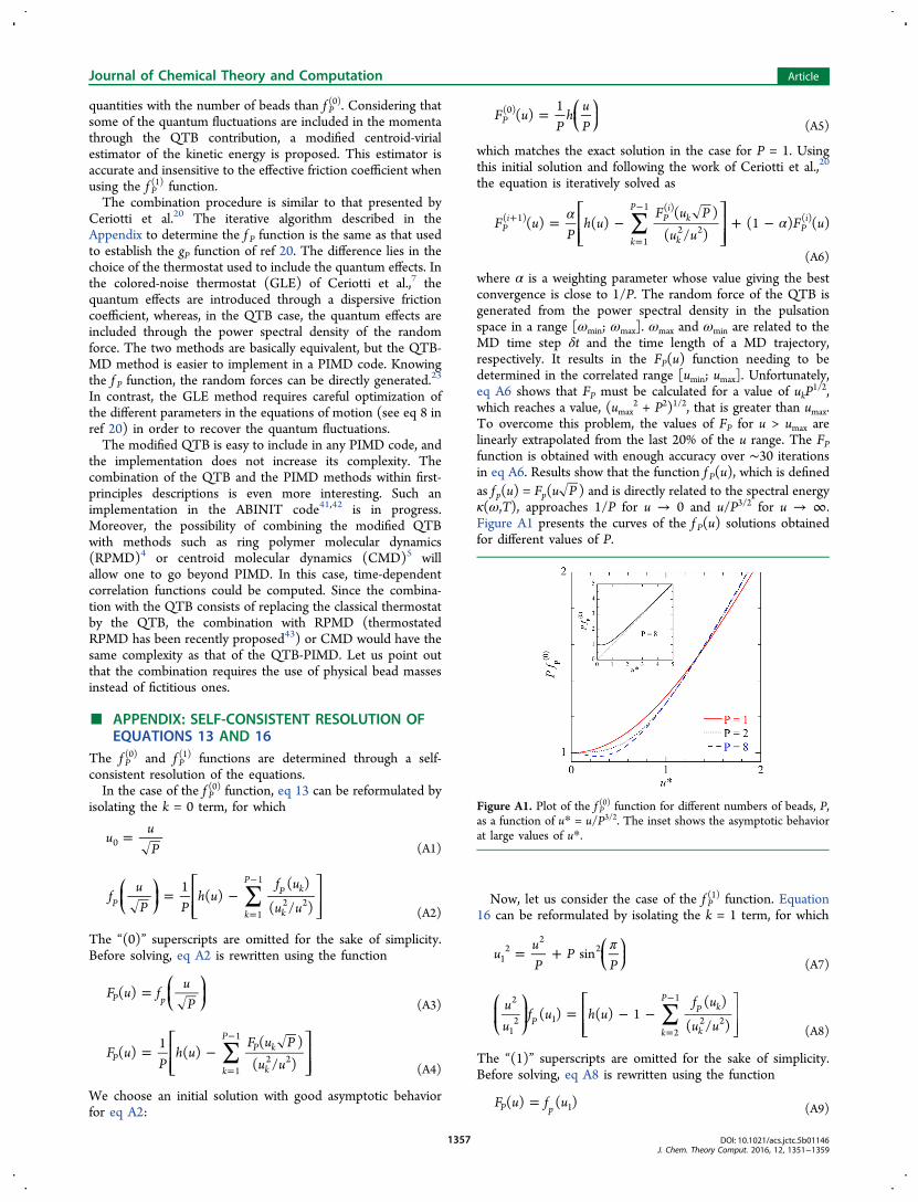
where α is a weighting parameter whose value giving the bestconvergence is close to 1/P. The random force of the QTB isgenerated from the power spectral density in the pulsationspace in a range [ωmin; ωmax]. ωmax and ωmin are related to theMD time step δt and the time length of a MD trajectory,respectively. It results in the FP(u) function needing to bedetermined in the correlated range [umin; umax]. Unfortunately,eq A6 shows that FP must be calculated for a value of ukP

1/2,which reaches a value, (umax

2 + P2)1/2, that is greater than umax.To overcome this problem, the values of FP for u > umax arelinearly extrapolated from the last 20% of the u range. The FPfunction is obtained with enough accuracy over ∼30 iterationsin eq A6. Results show that the function f P(u), which is definedas f p(u) = Fp(u P ) and is directly related to the spectral energyκ(ω,T), approaches 1/P for u → 0 and u/P3/2 for u → ∞.Figure A1 presents the curves of the f P(u) solutions obtainedfor different values of P.

Now, let us consider the case of the f P(1) function. Equation

16 can be reformulated by isolating the k = 1 term, for which

π= + ⎜ ⎟⎛⎝

⎞⎠u

uP

PP

sin12

22

(A7)

∑= − −=

−⎛⎝⎜

⎞⎠⎟

⎡⎣⎢⎢

⎤⎦⎥⎥

uu

f u h uf u

u u( ) ( ) 1

( )

( / )Pk

PP k

k

2

12 1

2

1

2 2(A8)

The “(1)” superscripts are omitted for the sake of simplicity.Before solving, eq A8 is rewritten using the function

=F u f u( ) ( )P p 1 (A9)

Figure A1. Plot of the f P(0) function for different numbers of beads, P,

as a function of u* = u/P3/2. The inset shows the asymptotic behaviorat large values of u*.

Journal of Chemical Theory and Computation Article

DOI: 10.1021/acs.jctc.5b01146J. Chem. Theory Comput. 2016, 12, 1351−1359

1357

∑ π= − − −=

−⎜ ⎟

⎡⎣⎢⎢

⎛⎝⎜

⎞⎠⎟

⎛⎝⎜⎜ ⎛

⎝⎞⎠

⎞⎠⎟⎤⎦⎥⎥F u

uu

h uuu

F Pu PP

( ) ( ) 1 sinPk

P

kP k

12

22

1 2

22 2 2

(A10)

We choose an initial solution with good asymptotic behaviorfor eq A8:

=−

−⎜ ⎟⎡⎣⎢

⎛⎝

⎞⎠

⎤⎦⎥F u

Ph

uP P

( )1

11

P(0)

(A11)

Using this initial solution, the equation is iteratively solved as

∑α

π α

= − −

− + −

+

=

−

⎜ ⎟

⎛⎝⎜

⎞⎠⎟⎡⎣⎢⎢

⎛⎝⎜

⎞⎠⎟

⎛⎝⎜⎜ ⎛

⎝⎞⎠

⎞⎠⎟⎤⎦⎥⎥

F uuu

h u uu

F Pu PP

F u

( ) ( ) 1

sin (1 ) ( )

Pi

k

P

k

P k Pi

( 1) 12

22

1 2

2

2 2 2 ( )

(A12)

where α is a weighting parameter whose value giving the bestconvergence is close to 1/P. The FP(u) function is determinedfollowing the above-mentioned procedure. Results show thatthe function

π= − ⎜ ⎟⎛⎝⎜⎜ ⎛

⎝⎞⎠

⎞⎠⎟f u F Pu P

P( ) sinP P

2 2 2

(A13)

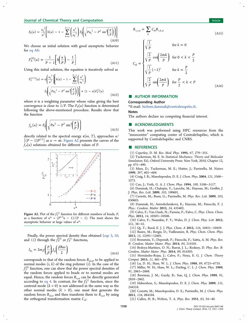
directly related to the spectral energy κ(ω, T), approaches u/[(P − 1)P1/2] as u → ∞. Figure A2 presents the curves of thef P(u) solutions obtained for different values of P.

Finally, the power spectral density thus obtained (eqs 3, 10,and 12) through the f P

(0) or f P(1) functions,

γβ

β ω= ℏ⎜ ⎟⎛⎝⎜

⎞⎠⎟

⎛⎝

⎞⎠I m

Pf2

2R i Pi (A14)

corresponds to that of the random forces Ri,k,α, to be applied tonormal modes (i, k) of the ring polymer (i). In the case of thef P(0) function, one can show that the power spectral densities ofthe random forces applied to beads or to normal modes areequal. Hence, the random forces Ri,s,α can be directly generatedaccording to eq 4. In contrast, for the f P

(1) function, since thecentroid mode (k = 0) is not addressed in the same way as theother normal modes (k > 0), one must first generate therandom forces Ri,k,α and then transform them to Ri,s,α by usingthe orthogonal transformation matrix Csk:

∑=α αR C Ri sk

sk i k, , , ,(A15)

π

π

=

=

< <

− =

< <

⎜ ⎟

⎜ ⎟

⎧

⎨

⎪⎪⎪⎪⎪

⎩

⎪⎪⎪⎪⎪

⎛⎝

⎞⎠

⎛⎝

⎞⎠

C

Pk

Psk

Pk

P

Pk

P

Psk

PP

k P

1for 0

2cos

2for 0

2

1( 1) for

2

2sin

2for

2

sks

(A16)

■ AUTHOR INFORMATIONCorresponding Author*E-mail: hichem.dammak@centralesupelec.fr.NotesThe authors declare no competing financial interest.

■ ACKNOWLEDGMENTSThis work was performed using HPC resources from the”mesocentre” computing center of CentraleSupelec, which issupported by CentraleSupelec and CNRS.

■ REFERENCES(1) Ceperley, D. M. Rev. Mod. Phys. 1995, 67, 279−355.(2) Tuckerman, M. E. In Statistical Mechanics: Theory and MolecularSimulation; Ed.; Oxford University Press: New York, 2010, Chapter 12,pp 475−490.(3) Marx, D.; Tuckerman, M. E.; Hutter, J.; Parrinello, M. Nature1999, 397, 601−604.(4) Craig, I. R.; Manolopoulos, D. E. J. Chem. Phys. 2004, 121, 3368−3373.(5) Cao, J.; Voth, G. A. J. Chem. Phys. 1994, 100, 5106−5117.(6) Dammak, H.; Chalopin, Y.; Laroche, M.; Hayoun, M.; Greffet, J.J. Phys. Rev. Lett. 2009, 103, 190601.(7) Ceriotti, M.; Bussi, G.; Parrinello, M. Phys. Rev. Lett. 2009, 103,030603.(8) Dammak, H.; Antoshchenkova, E.; Hayoun, M.; Finocchi, F. J.Phys.: Condens. Matter 2012, 24, 435402.(9) Calvo, F.; Van-Oanh, N.; Parneix, P.; Falvo, C. Phys. Chem. Chem.Phys. 2012, 14, 10503−10506.(10) Calvo, F.; Naumkin, F. Y.; Wales, D. J. Chem. Phys. Lett. 2012,551, 38−41.(11) Qi, T.; Reed, E. J. J. Phys. Chem. A 2012, 116, 10451−10459.(12) Basire, M.; Borgis, D.; Vuilleumier, R. Phys. Chem. Chem. Phys.2013, 15, 12591−12601.(13) Bronstein, Y.; Depondt, P.; Finocchi, F.; Saitta, A. M. Phys. Rev.B: Condens. Matter Mater. Phys. 2014, 84, 214101.(14) Bedoya-Martínez, O. N.; Barrat, J. L.; Rodney, D. Phys. Rev. B:Condens. Matter Mater. Phys. 2014, 89, 014303.(15) Hernandez-Rojas, J.; Calvo, F.; Noya, E. G. J. Chem. TheoryComput. 2015, 11, 861−870.(16) Lu, D. H.; Hase, W. L. J. Chem. Phys. 1988, 89, 6723−6735.(17) Miller, W. H.; Hase, W. L.; Darling, C. L. J. Chem. Phys. 1989,91, 2863−2868.(18) Bowman, J. M.; Gazdy, B.; Sun, Q. J. Chem. Phys. 1989, 91,2859−2862.(19) Habershon, S.; Manolopoulos, D. E. J. Chem. Phys. 2009, 131,244518.(20) Ceriotti, M.; Manolopoulos, D. E.; Parrinello, M. J. Chem. Phys.2011, 134, 084104.(21) Callen, H. B.; Welton, T. A. Phys. Rev. 1951, 83, 34−40.

Figure A2. Plot of the f P(1) function for different numbers of beads, P,

as a function of u* = (P1/2u − 1)/(P − 1). The inset shows theasymptotic behavior at large values of u*.

Journal of Chemical Theory and Computation Article

DOI: 10.1021/acs.jctc.5b01146J. Chem. Theory Comput. 2016, 12, 1351−1359

1358

(22) Kubo, R. Rep. Prog. Phys. 1966, 29, 255−284.(23) Chalopin, Y.; Dammak, H.; Laroche, M.; Hayoun, M.; Greffet, J.J. Phys. Rev. B: Condens. Matter Mater. Phys. 2011, 84, 224301.(24) Ceriotti, M.; Manolopoulos, D. E. Phys. Rev. Lett. 2012, 109,100604.(25) The f P function is different from the gP function of Ceriotti etal.20 because the authors used another formulation of the PIMD (attemperature P × T). Indeed, f P(u) = (1/P)gP(uP

1/2).(26) Herman, M. F.; Bruskin, E. J.; Berne, B. J. J. Chem. Phys. 1982,76, 5150−5155.(27) Parrinello, M.; Rahman, A. J. Chem. Phys. 1984, 80, 860−867.(28) Barrozo, A. H.; de Koning, M. Phys. Rev. Lett. 2011, 107,198901.(29) Dammak, H.; Hayoun, M.; Chalopin, Y.; Greffet, J. J. Phys. Rev.Lett. 2011, 107, 198902.(30) Young, R. A., Ed. In The Rietveld Method; Oxford UniversityPress: Oxford, U.K., 1993.(31) Zhong, W.; Vanderbilt, D. Phys. Rev. B: Condens. Matter Mater.Phys. 1996, 53, 5047−5050.(32) Iniguez, J.; Vanderbilt, D. Phys. Rev. Lett. 2002, 89, 115503.(33) Zhong, W.; Vanderbilt, D.; Rabe, K. Phys. Rev. B: Condens.Matter Mater. Phys. 1995, 52, 6301−6312.(34) Geneste, G.; Dammak, H.; Thiercelin, M.; Hayoun, M. Phys.Rev. B: Condens. Matter Mater. Phys. 2013, 87, 014113.(35) Azad, A. M.; Subramaniam, S. Mater. Res. Bull. 2002, 37, 85−97.(36) Akbarzadeh, A. R.; Kornev, I.; Malibert, C.; Bellaiche, L.; Kiat, J.M. Phys. Rev. B: Condens. Matter Mater. Phys. 2005, 72, 205104.(37) Kreuer, K. D. Annu. Rev. Mater. Res. 2003, 33, 333−359.(38) Colomban, P., Ed. In Proton Conductors: Solids, Membranes andGelsMaterials and Devices; Cambridge University Press: Cambridge,U.K., 1992; Part V.(39) Raiteri, P.; Gale, J. D.; Bussi, G. J. Phys.: Condens. Matter 2011,23, 334213.(40) Ottochian, A.; Dezanneau, G.; Gilles, C.; Raiteri, P.; Knight, C.;Gale, J. D. J. Mater. Chem. A 2014, 2, 3127−3133.(41) Gonze, X.; et al. Comput. Phys. Commun. 2009, 180, 2582−2615.(42) Geneste, G.; Torrent, M.; Bottin, F.; Loubeyre, P. Phys. Rev. Lett.2012, 109, 155303.(43) Rossi, M.; Ceriotti, M.; Manolopoulos, D. E. J. Chem. Phys.2014, 140, 234116.

Journal of Chemical Theory and Computation Article

DOI: 10.1021/acs.jctc.5b01146J. Chem. Theory Comput. 2016, 12, 1351−1359

1359