Embed Size (px)
Citation preview
Quantum Walks: A Markovian Perspective
Diego de Falco1,2 and Dario Tamascelli1,2
1 Dipartimento di Scienze dell’Informazione, Universita degli Studi di Milano,Via Comelico 39/41, 20135 Milano, Italy
2 CIMAINA, Centro Interdipartimentale Materiali e Interfacce Nanostrutturati,Universita degli Studi di Milano
Abstract. For a continuous-time quantum walk on a line the varianceof the position observable grows quadratically in time, whereas, for itsclassical counterpart on the same graph, it exhibits a linear, diffusive,behaviour. A quantum walk, thus, propagates at a rate which is linear intime, as compared to the square root rate for a classical random walk.Indeed, it has been suggested that there are graphs that can be traversedby a quantum walker exponentially faster than by the classical randomanalogue. In this note we adopt the approach of exploring the condi-tions to impose on a Markov process in order to emulate its quantumcounterpart: the central issue that emerges is the problem of taking intoaccount, in the numerical generation of each sample path, the causativeeffect of the ensemble of trajectories to which it belongs. How to dealnumerically with this problem is shown in a paradigmatic example.
Keywords: continuous-time quantum walks, birth-and-death processes,sample paths.
1 Paradigmatic Examples
The identity+∞∑
x=−∞Jx(t)2 = 1, (1)
satisfied by the Bessel functions of first kind and integer order Jx(t), shows thatthe function
ρ(t, x) = Jx(t)2 (2)
is, for each time t, a probability mass function on the relative integers.We raise here the question of finding examples of phenomena of probabilistic
time evolution described by this probability mass function.We will give two distinct, apparently very different, answers to the above
question: finding the relationship between the two distinct examples we are goingto exhibit below and discussing the extent and generality of this relationship willbe the main focus of this paper.
V. Geffert et al. (Eds.): SOFSEM 2008, LNCS 4910, pp. 519–530, 2008.c© Springer-Verlag Berlin Heidelberg 2008

520 D. de Falco and D. Tamascelli
t
x
30
�30
0
0 30
Fig. 1. A density plot of ρ(t, x) = |ψ(t, x)|2. The profile of ρ(30, x) as a function of xis shown on the right.
Example 1. The functionψ(t, x) = ixJx(t) (3)
is the solution of the Schrodinger equation on the relative integers
id
dtψ(t, x) = −1
2(ψ(t, x − 1) + ψ(t, x + 1)) (4)
under the initial conditionψ(0, x) = δ0,x. (5)
Otherwise stated, the function ρ(t, x) = Jx(t)2 is, at every time t, the probabilitydistribution of a continuous-time quantum walk on the graph having the relativeintegers as vertices, with edges between nearest neighbour sites [1]. This quantumwalk starts at time 0 from the origin.
Figure 1, a density plot of ρ(t, x) = Jx(t)2, clearly shows the linear propagationexpected in such a quantum walk. The reader more intersted in the phenomenonthan in the equation (in this case eq. (4)) will appreciate recognizing in figure 1the intensity pattern of propagation of light in a waveguide lattice [2].
Example 2. Consider a birth-and-death random process q(t) on the relative in-tegers, evolving according to the following rules:

Quantum Walks: A Markovian Perspective 521
i. geometric mean rule: for every edge {x, x+1} and every time t the fraction oftransitions per unit time taking place along this edge (number of transitionsx → x+1 plus number of transitions x+1 → x per unit time)/(sample size)is equal to the geometric mean of the probability of the process being in xand the probability of being in x + 1;
ii. local unidirectionality rule: for every edge {x, x+1}, and depending on timet, only transitions x → x + 1 or only transitions x + 1 → x are allowed;
iii. “horror vacui” rule: for every site x, if at a time tx the probability of beingin x passes through the value 0, then there is an interval of time following txin which along the edges {x − 1, x} and {x, x + 1} only transitions toward xare allowed; this time interval terminates as soon as the probability of beingin one of the two neighbours of x crosses the value 0 (at which instant the“horror vacui” rule takes hold for such a neighbour).
As to the initial conditions, we suppose that there exists τ0 > 0 such that, forevery integer x,
ρ(t, x) ≡ P (q(t) = x) > 0, for 0 < t < τ0 (6)
andlim
t→0+ρ(t, x) = δ0,x. (7)
Together with the above initial condition on the position of the process, weimpose, as a condition on its initial “velocity”, the requirement that in thetime interval [0, τ0) only transitions taking the process away from the origin areallowed.
We, finally, impose a left-right symmetry on the position of the process, inthe form
ρ(t, x) = ρ(t, −x) (8)
and a left-right symmetry on its “velocity” expressed in terms of its birth rateλ(t, x) and its death rate μ(t, x) as
λ(t, x) = μ(t, −x). (9)
The transition probabilities per unit time λ(t, x) and μ(t, x) are defined, re-spectively, by
p(t + τ, x + 1; t, x) = τ · λ(t, x) + o(τ) (10)
p(t + τ, x − 1; t, x) = τ · μ(t, x) + o(τ) (11)
for τ → 0+.Here and elsewhere we indicate by p(t, x; t0, x0) the conditional probability
P (q(t) = x|q(t0) = x0)
of finding the process at time t in x, given that at time t0 it is in x0.

522 D. de Falco and D. Tamascelli
Condition (i) can, now, be written as the equation
λ(t, x)ρ(t, x) + μ(t, x + 1)ρ(t, x + 1) =√
ρ(t, x)ρ(t, x + 1), (12)
relating the three unknown fields λ, μ and ρ. The left hand side is, indeed, theprobability per unit time of a transition along the link {x, x + 1}. Notice that,because of (ii), equation (12) allows, locally, to express λ or μ as a function ofthe values of ρ at two neighbouring points.
A further equation involving the unknown fields is the continuity equation
d
dtρ(t, x) = (μ(t, x + 1)ρ(t, x + 1) − λ(t, x)ρ(t, x)) + (13)
+ (λ(t, x − 1)ρ(t, x − 1) − μ(t, x)ρ(t, x)),
expressing the fact that the probability mass at x increases because of transitionsx ± 1 → x and decreases because of transitions x → x ± 1.
In the time interval [0, τ0), we can therefore write, using also the left-rightsymmetry and the initial condition of allowing only transitions taking the processaway from the origin (namely, for 0 ≤ t < τ0, λ(t, x) > 0 for x ≥ 0 and μ(t, x) > 0for x ≤ 0),
d
dtρ(t, 0) = −2
√ρ(t, 0)ρ(t, 1) (14a)
d
dtρ(t, x) = +
√ρ(t, x − 1)ρ(t, x) −
√ρ(t, x)ρ(t, x + 1), for x > 0. (14b)
Equations (14) are satisfied by ρ(t, x) = Jx(t)2, for values of t such that Jx(t)is positive for every non negative integer x. This determines the numerical valueof τ0 to be the smallest positive solution of the equation J0(t) = 0, namely
τ0 = 2.4048. (15)
For a suitable value of τ1 > τ0 condition (iii) will allow, in the time interval[τ0, τ1), for transitions ±1 → 0, so that equations (14) are to be substituted, inthis interval, by
d
dtρ(t, 0) = +2
√ρ(t, 0)ρ(t, 1), (16a)
d
dtρ(t, 1) = −
√ρ(t, 0)ρ(t, 1) −
√ρ(t, 2)ρ(t, 1) (16b)
d
dtρ(t, x) = +
√ρ(t, x − 1)ρ(t, x) −
√ρ(t, x)ρ(t, x + 1), for x > 1. (16c)
Equations (16) are again satisfied by ρ(t, x) = Jx(t)2, but, this time, for valuesof t such that J0(t) < 0 and Jx(t) is positive for every positive integer x. Thisdetermines the numerical value of τ1 to be the smallest positive root of J1(t) = 0,namely
τ1 = 3.8317. (17)

Quantum Walks: A Markovian Perspective 523
The above considerations can be iterated: using the fact that between two con-secutive zeroes of Jx(t) there is one and only one zero of Jx+1(t), one can controlthe changes of sign determined by (iii) in the continuity equation, to the effect ofproving that the process q(t) described by the conditions posed above satisfies,for every t, the condition
ρ(t, x) ≡ P (q(t) = x) = Jx(t)2. (18)
Figure 2, to be compared with figure 1, shows a few sample paths of theprocess q(t).
30t
�30
0
30
x
Fig. 2. A sample of 500 paths of the stochastic process of Example 2. For the purposeof comparison with figure 1, the empirical distribution at time t = 30, of a sample of5 · 104 trajectories, is shown on the right.
The reader more interested in the phenomenon than in the equations (in thiscase the continuity equation (13) for the evolution of ρ(t, x) and the forwardKolmogorov equation for the evolution of p(t, x; t0, x0)) will see, in section 3,how the numerical procedure leading to figure 2 actually makes use only of astep by step implementation of the dynamical rules (i), (ii), (iii).
2 Quantum Walks vs. Random Walks
In this section we look at quantum mechanics as a metaphor suggesting, atthe heuristic level, an interesting dynamical behaviour for a random (Markov)

524 D. de Falco and D. Tamascelli
process exploring a graph or decision tree. We base our work on the classicalresults of Guerra and Morato [3] on the formulation of quantum-mechanical be-haviour in terms of controlled stochastic processes; the picture of a quantumwalk that emerges through its stochastic analogue is that of a swarm of walk-ers moving according to transition rules involving the distribution of the entireswarm.
Consider a quantum system having as state space a Hilbert space the dimen-sion of which we will indicate by s, and as generator of the time evolution aHamiltonian operator that we will indicate by H .
Having fixed an orthonormal basis, |φ1 〉, |φ2 〉, . . . , |φs 〉, a graph G is defined,starting from the selected basis and from the selected Hamiltonian, by statingthat G has Λs = {1, ...., s} as its set of vertices and edges {k, j} such that j �= kand |〈 φk |H | φj 〉| > 0.
In the context of this section, the graph G will play the role played, in themore elementary context of Example 1 of section 1, by the linear graph havingthe relative integers as vertices, with edges between nearest neighbour sites.Similarly, the role played in section 1 by equation (4) will be played in thissection by the Schrodinger equation in the representation determined by theselected basis:
id
dtψ(t, k) =
s∑
j=1
Hk,j · ψ(t, j) (19)
withHk,j = 〈 φk |H | φj 〉. (20)
We pose in the following terms the question of finding in the general context ofthis section, an analogue of Example 2 of section 1:
Easy problem: find a constructive procedure associating with each solution ψ of(19) a Markov process q(t) on the graph G having at each time t probabilitydistribution
ρ(t, k) = P (q(t) = k) = |ψ(t, k)|2. (21)
If this process exists and satisfies (for a suitable field ν of transition probabilitiesper unit time) the condition, that we impose as an analogue of conditions (10)and (11),
p(t + τ, j; t, k) ≡ P (q(t + τ) = j|q(t) = k) = τ · νj(t, k) + o(τ) (22)
for τ → 0+ and for each j being a neighbour of k in the graph G, then it willsatisfy the continuity equation
d
dtρ(t, k) =
∑
j∈N(k)
ρ(t, j)νk(t, j) − ρ(t, k)νj(t, k) = (23)
=∑
j∈N(k)
(ρ(t, j)νk(t, j) + ρ(t, k)νj(t, k))(
ρ(t, j)νk(t, j) − ρ(t, k)νj(t, k)ρ(t, j)νk(t, j) + ρ(t, k)νj(t, k)
).

Quantum Walks: A Markovian Perspective 525
In the above equation, we have indicated by N(k) the set of neighbours in Gof the vertex k, namely the collection of vertices j such that j �= k and {j, k} isan edge.
In the second line of equation (23) we have separated the term
ρ(t, j)νk(t, j) + ρ(t, k)νj(t, k),
symmetric in j and k (on the analogue of which we have imposed in Section 1the geometric mean rule), from the antisymmetric term
ρ(t, j)νk(t, j) − ρ(t, k)νj(t, k)ρ(t, j)νk(t, j) + ρ(t, k)νj(t, k)
,
of absolute value ≤ 1, representing the net relative flux of probability mass fromj into k.
If, now, the same ρ appearing in (23) satisfies also ρ(t, k) = |ψ(t, k)|2 for a ψsatisfying (19), it must be
ψ(t, k) =√
ρ(t, x) exp(i · S(t, k)) (24)
for some phase function S to be determined by inserting the Ansatz (24) intoequation (19). Doing so, and separating the real and imaginary parts of theresulting equation, one gets two equations:
d
dtS(t, k) = −Hk,k −
∑
j∈N(k)
hk,j
√ρ(t, j)ρ(t, k)
cos(βk,j(t)) (25)
andd
dtρ(t, k) =
∑
j∈N(k)
2hk,j
√ρ(t, k)ρ(t, j) sin(βk,j(t)), (26)
where we have sethk,j = |Hk,j | (27)
andβk,j(t) = Arg(Hk,j) + S(t, j) − S(t, k). (28)
In order to check that our Easy problem admits at least one solution, it issufficient to compare the purely kinematic relations
d
dtρ(t, k) =
∑
j∈N(k)
2hk,j
√ρ(t, k)ρ(t, j) sin(βk,j(t)),
and
d
dtρ(t, k) =
∑
j∈N(k)
(ρ(t, j)νk(t, j)+ρ(t, k)νj(t, k))(
ρ(t, j)νk(t, j) − ρ(t, k)νj(t, k)ρ(t, j)νk(t, j) + ρ(t, k)νj(t, k)
),

526 D. de Falco and D. Tamascelli
viewed, for assigned ψ and therefore for assigned ρ and β, as constraints onthe unknown transition probabilities per unit time of the process q(t) to beconstructed. The simplest way to satisfy this constraint is by requiring term byterm equality in the sums that appear in the right hand sides, and by equatingin each term the symmetric and antisymmetric factors.
We thus get the equations
ρ(t, j)νk(t, j) + ρ(t, k)νj(t, k) = 2hk,j
√ρ(t, k)ρ(t, j) (29)
ρ(t, j)νk(t, j) − ρ(t, k)νj(t, k) = 2hk,j
√ρ(t, k)ρ(t, j) sin(βk,j(t)) (30)
that are solved by
νk(t, j) = hk,j
√ρ(t, k)ρ(t, j)
(1 + sin(βk,j(t))) =
= hk,j
√ρ(t, k)ρ(t, j)
(1 + sin(Arg(Hk,j) + S(t, j) − S(t, k))) (31)
for k ∈ N(j).For more details, and for the physical motivation (related to questions of time
reversal invariance) of the merits of this particular choice, we refer to [4].It is immediate to check that (29) is precisely the geometric mean rule (i) of
section 1.It is also an easy exercise to check that (31) specializes, due to the phase factor
ix in equation (3), to conditions (ii) and (iii) in the simple context of section 1.
3 Autonomous Generation
The Hard problems, as opposed to the kinematical Easy problem reviewed insection 2, are
I. understand (25) as a dynamical condition on the processes q(t) that solveour Easy problem;
II. autonomously simulate these processes by actual implementation of this dy-namical condition.
Problem I is discussed in full detail in [4] following the general approach of [3] inwhich stochastic control theory is successfully proposed as a very simple modelsimulating quantum-mechanical behaviour.
We are not able to tackle problem (II) in its generality. We can only go backto section 1 and show that the three dynamical rules and the initial conditionsstated there in assigning Example 2 are enough to generate the sample paths offigure 2.
This is far from obvious because of the geometric mean rule: it requires, inthe numerical generation of each sample path, to take into account the causativeeffect (through the estimated probability distribution) on each trajectory of theensemble of trajectories to which it belongs [5] .

Quantum Walks: A Markovian Perspective 527
Even to show, as in figure 2, a small sample of trajectories, the need of carefullyestimating at each time step the density ρ imposes the simultaneous generationof a large number Ntr. of trajectories.
The numerical procedure leading to figure 2, makes, by purpose, no refer-ence to the solution of the continuity equation we have given in section 1, norto the solution of the Kolmogorov equations for the conditional probabilitiesp(t, x; t0, x0) that can be easily found by similar techniques. We present herethis procedure in some detail because the challenges one meets in simulating theprocess q(t) by implementing rules (i), (ii), (iii) and the initial conditions listedin section 1 give an operational meaning to the notion of autonomous simulation.
The state of the system at each time t = τ · k, where the integer k runs from1 to nsteps and τ is the time step, is described by the pair
– configuration array of length Ntr: its j-th element qj(t) indicates the cur-rent position of the j-th trajectory; a space cut-off is introduced throughan integer parameter L such that each trajectory is followed as long as−L ≤ q(t) ≤ L; the empirical density ρemp of the process at each time isestimated from the configuration array;
– transition array indexed from −L to L: its x-th element is an ordered pairof bits (mx, lx): if mx = 1 (resp. lx = 1) then transitions x → x − 1 (resp.x → x+ 1) are allowed, whereas if mx = 0 (resp. lx = 0) they are forbidden.
In our implementation ntr. = 5 · 104, τ = 0.05, and the process has beenfollowed up to time tmax = τ ·nsteps = 100, well beyond the time window shownin figure 2; the space cut-off has been set at L = 150.
The algorithm consists of the iteration nsteps times of the following steps:
1. estimate ρemp from the configuration array;2. increment each qj(t) by Move(t, qj(t)), where the random variable Move(t, x)
takes the values −1, 0, +1 with probabilities τ ·μemp(t, x), 1−τ · (μemp(t, x)+λemp(t, x)), τ · λemp(t, x), respectively.
The empirical transition rates λemp and μemp are here given by
λemp(t, x) =
√ρemp(t, x + 1)
ρemp(t, x)lx; (32a)
μemp(t, x) =
√ρemp(t, x − 1)
ρemp(t, x)mx, (32b)
3. estimate the new empirical distribution ρemp(t + τ, x);4. if ρemp(t, x) > 0 and ρemp(t + τ, x) = 0 then update the transition array
following the “horror vacui” rule (iii), namely setting lx−1 = 1 and mx+1 =1, and restore the local unidirectionality rule by setting (mx, lx) = (0, 0).
In the initialization step the transition array has been given the initial assign-ment
(mx, lx) =
⎧⎪⎨
⎪⎩
(1, 0) if x < 0(1, 1) if x = 0(0, 1) if x > 0
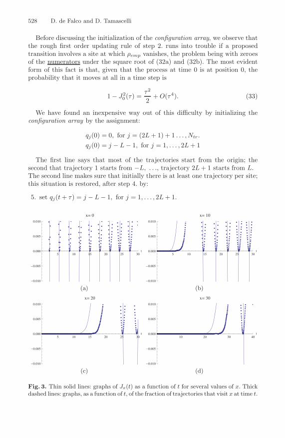
528 D. de Falco and D. Tamascelli
Before discussing the initialization of the configuration array, we observe thatthe rough first order updating rule of step 2. runs into trouble if a proposedtransition involves a site at which ρemp vanishes, the problem being with zeroesof the numerators under the square root of (32a) and (32b). The most evidentform of this fact is that, given that the process at time 0 is at position 0, theprobability that it moves at all in a time step is
1 − J20 (τ) =
τ2
2+ O(τ4). (33)
We have found an inexpensive way out of this difficulty by initializing theconfiguration array by the assignment:
qj(0) = 0, for j = (2L + 1) + 1 . . . , Ntr.
qj(0) = j − L − 1, for j = 1, . . . , 2L + 1
The first line says that most of the trajectories start from the origin; thesecond that trajectory 1 starts from −L, . . ., trajectory 2L + 1 starts from L.The second line makes sure that initially there is at least one trajectory per site;this situation is restored, after step 4. by:
5. set qj(t + τ) = j − L − 1, for j = 1, . . . , 2L + 1.
5 10 15 20 25 30t
�0.010
�0.005
0.000
0.005
0.010
x� 0
(a)
5 10 15 20 25 30t
�0.010
�0.005
0.000
0.005
0.010
x� 10
(b)
5 10 15 20 25 30t
�0.010
�0.005
0.000
0.005
0.010
x� 20
(c)
10 20 30 40t
�0.010
�0.005
0.000
0.005
0.010
x� 30
(d)
Fig. 3. Thin solid lines: graphs of Jx(t) as a function of t for several values of x. Thickdashed lines: graphs, as a function of t, of the fraction of trajectories that visit x at time t.

Quantum Walks: A Markovian Perspective 529
The dummy trajectories labelled by j = 1, . . . , 2L+1 provide some probabilitymass when needed to prevent the first order procedure from getting stuck.
Comparison between figures 1 and 2 gives an idea of how well our simpleprocedure fills the configuration array .
An analogous comparison is conducted in figure 3 for the transition array:the issue there is how well our procedure catches the instants of time at whichthe control mechanism expressed by the “horror vacui” rule takes hold, namelythe zeroes of Jx(t).
4 Conclusions and Outlook
If you give me a quantum walk efficiently exploring a graph or decision tree [6],I take your computational basis, your initial condition and your Hamiltonianand cook for you a stochastic process by computing its transition probabilitiesper unit time according to the recipe of section 2 and its transition probabilitiesp(t, x; t0, x0) by integration of the Kolmogorov equations (this can be done inquite explicit terms for the Example 2 of section 1) or by a clever exploitationof a few rules controlling the dynamics, as done in section 3. The discussion ofsection 2 makes it clear that my random walk will, by construction, visit yourgraph or decision tree as efficiently as your quantum walk.
Can the above statement be reconciled with the statement that the quantumglued trees algorithm of [7] outperforms any classical algorithm? How are theclassical alternatives defined in the original literature on exponential speedupby quantum walk? Does the causative effect of the ensemble disqualify a Markovprocess from being classical ?
On these points, all we can do is to advance a conjecture: the cost of myrandom simulation of your quantum walk is hidden in the size Ntr. of the sampleI am required to generate. We have indeed called attention, since section 1, onthe geometric mean rule: for every edge of your graph the probability per unittime of a transition of my process along that edge is equal to the geometric meanof the probabilities of the process at the two vertices joined by that edge.
We pose as a problem of future research the quantitative assessment of thecost (as measured by Ntr.) of the density estimation step required before eachupdating in the simulation.
References
1. Childs, A., Farhi, E., Gutmann, S.: An example of the difference between quantumand classical random walks. Quantum Information Processing 1, 35–43 (2002)
2. Perets, H., Lahini, Y., Pozzi, F., Sorel, M., Morandotti, R., Silberberg, Y.: Re-alization of quantum walks with negligible decoherence in waveguide lattices,arXiv:quant-ph/0707.0741v2 (2007)
3. Guerra, F., Morato, L.: Quantization of dynamical systems and stochastic controltheory. Phys. Rev. D 27, 1774–1786 (1983)
4. Guerra, F., Marra, R.: Discrete stochastic variational principles and quantum me-chanics. Phys. Rev. D 29(8), 1647–1655 (1984)

530 D. de Falco and D. Tamascelli
5. Smolin, L.: Could quantum mechanics be an approximation to another theory?,arXiv-quant-ph/0609109 (2006)
6. Farhi, E., Gutmann, S.: Quantum computation and decision trees. Phys. Rev. A 58,915–928 (1998)
7. Childs, A., Cleve, R., Deotto, E., Farhi, E., Gutmann, S., Spielman, D.: Exponentialalgorithmic speed up by quantum walk. In: STOC 2003. Proc. 35th ACM symp.,pp. 59–68 (2003)