79

TECHNISCHE MECHANIK, Band 24, Heft 2, (2004), 79-90 Manuskripteingang: 16. Dezember 2004

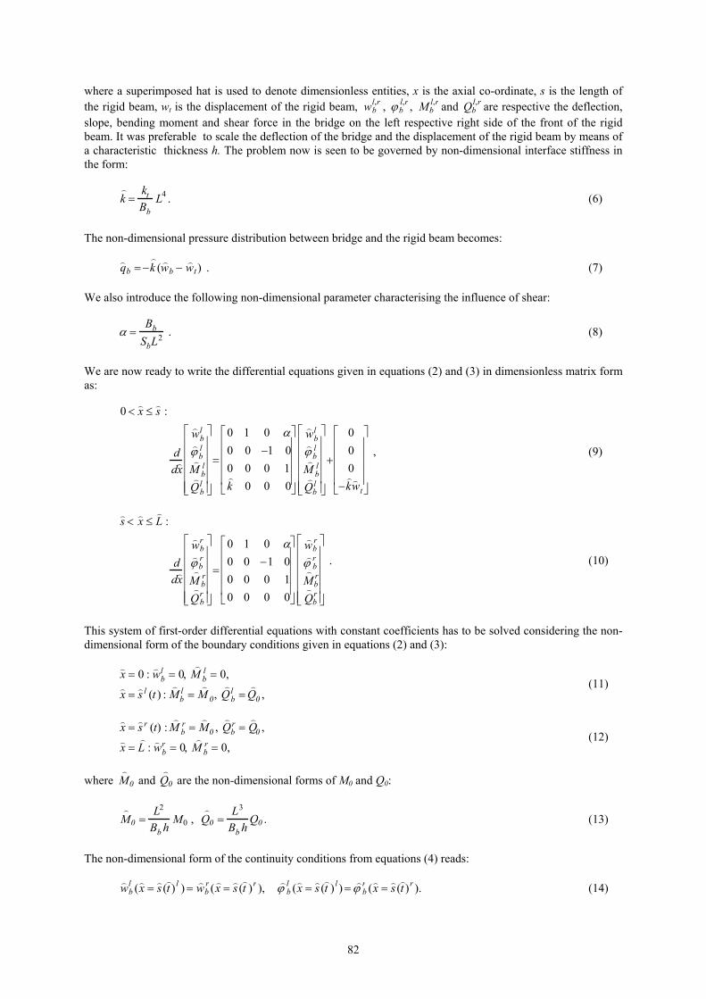
Quasi-static Response of a Timoshenko Beam Loaded by an Elastically Supported Moving Rigid Beam E. C. Cojocaru, J. Foo, H. Irschik The present paper is concerned with the quasi-static response of an elastic beam, loaded by a rigid beam, which is slowly transported along the elastic beam. The elastic beam is modelled as a Timoshenko beam. The present paper provides a limiting case of the model with constant distributed load that is often considered in the study of transported masses. The rigid beam is connected to the Timoshenko beam by means of an interface modelled as a Winkler foundation. We present a non-dimensional study on the influence of the interface stiffness upon the displacement, bending moment and shear force of the Timoshenko beam, when the rigid beam is assumed to suffer a prescribed transverse displacement. Special emphasis is laid on the distribution of pressure transmitted by the interface between the Timoshenko beam and the rigid beam. Considerable pressure concentrations are found to take place and the locations of the maximum bending moments in the Timoshenko beam move towards the ends of the rigid beam. 1 Introduction The response of elastic beams to moving distributed loads has been the subject of numerous investigations in various areas, such as the response of bridges to moving vehicles, or the transportation of masses along a carrier structure. The moving loads have been modelled at first as single force or mass, or as series of moving forces or moving masses. Often, force loading with constant distribution was used as a simplified model to study the response of the structure to the transported masses see Felszeghy (1996). When the interaction between the structure and the moving load is of interest, more complicated models, which consist of rigid bodies connected by springs and dampers, come into the play. An extensive review on the dynamic response of a beam acted on by moving loads or moving masses has been presented by Fryba (1999). An overview of the recent research work on vibration analysis of various types of bridges under action of moving vehicles and trains has been given by Au et al. (2001). In reality, the moving loads represent a structure with an own stiffness, which is connected to the carrying elastic beam by means of an interface. In the following, we treat the limiting case of a rigid beam that is slowly transported along a simply supported elastic beam. In order to account for shear deformations the carrying elastic beam is modelled in accordance with the theory of Timoshenko (1921). There are numerous important investigations that deal with the response of infinite or finite elastically supported Timoshenko beams or cantilever beams, which are acted by concentrated forces or masses, or on simply supported Timoshenko beams acted by constant or given line loads. In order to cite only a few of these contributions, we mention a general series solution for Timoshenko beams by Anderson (1953). Recently Antes (2003) proposed a boundary integral formulation for the static case as a first step to dynamic analysis of Timoshenko beam systems. For the influence of shear deformations on flexural waves see Graff (1975). An interesting study on the influences of the layer properties on the structural characteristics of a layered beam is discussed in Chen (1995). In our present model the rigid beam is connected to the Timoshenko beam by means of an interface (or layer) modelled as a Winkler (one-parameter) foundation, see Timoshenko (1926). The problem then is mainly governed by two stiffness parameters, the bending stiffness of the elastic beam, and the stiffness parameter of the interface. This model finds a direct application in the field of steel production, where a rigid metal slab is transported over a series of elastic rolls, the latter being attached to some elastic carrier beams. However, the present model should also be of interest for the motion of a train across a bridge. The rigid beam then represents the first (transverse rigid-body-motion) term in a series representation for the deformation of the train, and the Winkler foundation models the elastically supported wheels of the train.

80

The following study deals with the case of a quasi-static motion of the rigid beam. In the case of a fast motion, vibrations about the corresponding quasi-static response of the Timoshenko beam will take place. The latter dynamic response is intended to be treated in a future investigation. Here, we are interested in the following interesting phenomenon, which has been detected in our subsequent computations: When the rigid beam is assumed to obey a given transverse displacement, such that the interface is compressed, and when the bending stiffness of the Timoshenko beam is sufficiently small, then displacements, bending moments and shear forces are found to deviate strongly from their well-known distributions for the case of a line load with constant distribution. In contrast to the latter solutions, considerable pressure concentrations are seen to occur at the ends of the region covered by the rigid beam, and the locations of the maximum bending moments in the Timoshenko beam move towards the ends of this region. Moreover, when the stiffness of the Timoshenko beam is further decreased, the Winkler interface even must suffer tensile forces, or a lift-off is to be expected in some regions of the interface. In the following, this situation is described in a non-dimensional setting in order to cover all possible cases by a single formulation. Accordingly, the problem is formulated in the form of two sets of first-order ordinary differential equations, one set being valid for the unloaded part of the Timoshenko beam, the other for the region loaded by the rigid beam. The two sets are coupled by means of transition conditions valid at the location of the front of the rigid beam. The problem is solved for various locations of this front along the elastic beam, where we assume the rigid beam is long enough, such that only one front is to be considered. When the elastic beam would be modelled in the framework of the Bernoulli-Euler theory of beams, the non-dimensionalised problem were governed by a single similarity complex or Pi-number only, namely a non-dimensional interface stiffness formed by the ratio of the Winkler foundation stiffness and the bending stiffness of the elastic beam, as well as by the fourth power of the span of the elastic beam. For the notion of a Pi number in similarity methods of engineering dynamics, see e.g. Baker et al. (1991). In the present paper, we also take into account the influence of shear stiffness of the elastic beam according to the theory of Timoshenko (1921), such that a second Pi number comes into the play. Since the influence of the latter is small, it was kept fixed in all of the numerical computations. In order to derive and demonstrate the above cited effect of pressure concentration, we utilise the symbolic computer code Maple 7 for solving the fourth-order system of ordinary differential equations with span-wise constant coefficients, where we use methods of linear algebra, as described lucidly e.g. in the book of Luenberger (1979). The results of our study are presented graphically in a non-dimensional form as a function of the axial co-ordinate of the elastic beam for various values of the non-dimensional interface stiffness, and for three locations of the front of the rigid beam. Non-dimensional deflection, bending moments and shear forces are depicted, and special emphasis is laid on the pressure distribution between the elastic beam and the rigid beam. In order to prove the results of our symbolic computations we also developed a Finite Element model using the powerful code ABAQUS 6.2. The convergence behaviour of the Finite Element model turned out to depend on the type of modelling of the Winkler interface by discrete springs, however the results were almost identical to the results of the symbolic computation in all of the considered cases. 2 Rigid Beam on a Winkler Foundation Travelling on a Simply Supported Beam Consider a simply supported straight beam of length L that represents the elastic beam in our model. A subscript (b) is used to denote the corresponding mechanical entities see Figure 1a. We utilise the theory of Timoshenko (1921) to describe the deformation of the elastic beam. In the following, Bb=EbIb denotes the effective bending stiffness, Eb is the Young's modulus, Ib is the second moment of inertia of the cross-sectional area. The shear stiffness is given by Sb =γAbGb, where γ is the Timoshenko shear coefficient, Ab is the cross-sectional area and Gb denotes the shear modulus of the Timoshenko beam. This elastic beam is loaded by transverse forces qb. Deflection, slope, bending moment and shear force of the beam are denoted by wb, ϕb, Mb and Qb, respectively. In our problem, the transverse forces qb represents the pressure that is transmitted by an elastic interface from the moving rigid beam to the elastic beam see Figure 1b. The rigid beam is assumed to move slowly across the elastic beam, and to be displaced in transverse direction downwards to the Timoshenko beam. In order to fix ideas, the subscript (t) is used to denote the transverse displacement of the rigid beam, wt see Figure 1. For the sake of brevity, and in order to avoid ambiguities between the two beams under consideration, we call the Timoshenko beam the “bridge” in the following. That is why we have introduced the index b for the

81

Timoshenko beam. We model the transmitting interface by a Winkler foundation with stiffness parameter kt, such that:

qb = −kt wb − wt( ), (1) see Timoshenko (1926) and Knothe (2001). All of the mechanical entities under consideration are described as a function of the axial co-ordinate x measured in an inertial frame which has the origin at the left end of the bridge, see Figure 1a. The rigid beam is assumed to be semi-infinite and to travel slowly along the bridge, such that the front of the rigid beam is located at the distance s(t), also measured from the left end of the beam, see Figure 1a. a) b)

rigid beam

wt(t) kt

0 s(t)

x elastic beam, Bb, Sb L

rigid beam

qb=-kt(wb-wt) M0

Q0 Q0

s(t) L-s(t)

Figure 1. An elastic beam carrying a rigid elastically supported beam

In the co-ordinate system under consideration, the problem can be described by the following two boundary value problems of fourth order:

0 < x ≤ s(t) : dwb

l

dx= ϕb

l +Qb

l

Sb,

dϕ bl

dx= −

M bl

Bb,

dM bl

dx= Qb

l , dQb

l

dx= kt (wb

l − wt ),

x = 0 : wbl = 0, M b

l = 0,

x = s(t) l : M bl = M0 , Qb

l = Q0 .

(2)

s(t) < x ≤ L :

dwbr

dx= ϕb

r +Qb

r

Sb,

dϕ br

dx= −

M br

Bb,

dM br

dx= Qb

r , dQb

r

dx= 0,

x = s(t) r : M br = M0 , Qb

r = Q0,

x = L : wbr = 0, M b

r = 0 .

(3)

For details of the underlying beam theory, see Timoshenko (1921), Graff (1975) and Ziegler (1991). In equations (2) and (3), the superscripts l and r denote the regions on the left and right hand side of the front of the rigid beam, x=s(t). Bending moment and shear force in the bridge at this location is denoted as M0 and Q0, respectively. Since we are interested in a quasi-static solution, the influence of the velocity of the rigid beam, and thus any effect of inertia, has been neglected in equations (2) and (3). This allows to model the problem as a system of first-order ordinary differential equations. According to the force method, see Ziegler (1991), the additional unknowns M0 and Q0 are calculated from the following two conditions of kinematical continuity for the bridge at the location s(t):

wbl (x = s(t) l ) = wb

r (x = s(t ) r ), ϕbl (x = s (t) l ) = ϕ b

r (x = s(t) r ). (4) In order to work with the minimum number of parameters that determine the solution of the problem in hand, we introduce the following dimensionless formulations:

x = L) x , s = L) s , wt = h ) w t , wb

l,r = h ) w bl,r , ϕ b

l,r =hL

) ϕ bl,r , M b

l ,r =BbhL2

) M b

l,r , Qbl,r =

BbhL3

) Q b

l,r , (5)

82

where a superimposed hat is used to denote dimensionless entities, x is the axial co-ordinate, s is the length of the rigid beam, wt is the displacement of the rigid beam, wb

l,r , ϕbl,r , Mb

l,r and Qbl,r are respective the deflection,

slope, bending moment and shear force in the bridge on the left respective right side of the front of the rigid beam. It was preferable to scale the deflection of the bridge and the displacement of the rigid beam by means of a characteristic thickness h. The problem now is seen to be governed by non-dimensional interface stiffness in the form:

) k =

ktBb

L4 . (6)

The non-dimensional pressure distribution between bridge and the rigid beam becomes:

) q b = −

) k ( ) w b − ) w t ) . (7)

We also introduce the following non-dimensional parameter characterising the influence of shear:

α =Bb

SbL2 . (8)

We are now ready to write the differential equations given in equations (2) and (3) in dimensionless matrix form as:

0 < ) x ≤ ) s :

dd) x

) w bl

) ϕ bl

) M b

l)

Q bl

=

0 1 0 α0 0 −1 00 0 0 1) k 0 0 0

) w bl

) ϕ bl

) M b

l)

Q bl

+

000

−) k ) w t

, (9)

) s < ) x ≤) L :

dd) x

) w br

) ϕ br

) M b

r)

Q br

=

0 1 0 α0 0 −1 00 0 0 10 0 0 0

) w br

) ϕ br

) M b

r) Q b

r

. (10)

This system of first-order differential equations with constant coefficients has to be solved considering the non-dimensional form of the boundary conditions given in equations (2) and (3):

) x = 0 : ) w bl = 0,

) M b

l = 0, ) x = ) s l (t ) :

) M b

l =)

M 0, )

Q bl =

) Q 0 ,

(11)

) x = ) s r (t) :)

M br =

) M 0 ,

) Q b

r =) Q 0 ,

) x =) L : ) w b

r = 0, )

M br = 0,

(12)

where

) M 0 and

) Q 0 are the non-dimensional forms of M0 and Q0:

) M 0 =

L2

Bb hM0 ,

) Q 0 =

L3

Bb hQ0 . (13)

The non-dimensional form of the continuity conditions from equations (4) reads:

) w b

l () x = ) s () t ) l ) = ) w b

r ( ) x = ) s () t )r ), ) ϕ b

l () x = ) s () t ) l ) = ) ϕ b

r () x = ) s () t )r ). (14)

83

3 Solution by means of Symbolic Computation The boundary value problems presented in Section 2 were solved by means of the symbolic computer code Maple 7. For the left region of the bridge, loaded by the rigid beam, we solved the system of first-order differential equations (9) in terms of the boundary conditions (11) and the loads. The system of differential equations can be formally written as:

′ X = AX + bu , (15) where X denotes a state vector,

XT = ) w bl ) ϕ b

l ) M b

l ) Q b

l[ ] ,′ X T = d

d) x ) w b

l ) ϕ bl )

M bl )

Q bl[ ] ,

(16)

A is the 4×4 matrix of coefficients:

A =

0 1 0 α0 0 −1 00 0 0 1) k 0 0 0

, (17)

and b is the vector of external loads:

bT = 0 0 0 −1[ ] ,u =

) k ) w t .

(18)

Following Luenberger, the general solution of the system (15) is:

X( ) x ) = Φ() x )X(0) + Φ() x − τ ) b u (τ )dτ0

) x

∫ (19)

where τ is an independent variable. The first term on the right-hand side of equation (19) represents the response due to the state vector X( 0) . For systems with constant coefficients, the state-transition matrix is known to be of the form Φ( ) x ) = exp(A) x ) , see Luenberger (1979). In order to compute the state-transition matrix, the Laplace transform method was utilised:

).)p(()x( - 1−−= AI1L)Φ (20) I denotes the identity matrix, and p stands for the parameter of the Laplace transformation. We used Laplace transformation approach, since the direct computation of Φ( ) x ) by the command exponential of Maple 7 failed in our hands. We have been told that the corresponding computational problem will be corrected in future versions of Maple. Because the vector X( 0) is not entirely known, we used the boundary conditions (11) to compute the unknown terms in X( 0) as well as in X( ) s ) . For that sake, equation (19) is written for

) x = ) s :

X() s ) = Φ() s )X(0) + Φ () s − τ) b u(τ)dτ0

) s

∫ . (21)

84

The relation (21) reads in an ample form:

) w bl

) ϕ bl

) M 0) Q 0

) x = ) s

= Φ() s )

0) ϕ b

l

0)

Q bl

) x = 0

+ Φ() s −τ ) b u (τ )dτ0

) s

∫ , (22)

In the system (22), the unknowns are:

) ϕ b

l (0), )

Q bl (0), ) w b

l () s ), ϕbl () s ) . (23)

We have thus arrived at a system of four linear equations, the solution of which defines the vectors X( 0) and

X( ) s ) in equation (21), expressed as functions of

) M 0 and

) Q 0 .

To solve the above problem, we used the functions of two packages of the symbolic computer code Maple 7, see (2001): the inttrans Package that is a collection of functions designed to compute integral transforms, and the Linear Algebra Package that allows standard matrix manipulation. We created the matrix A and vectors XT, X’T and bT as a list of initial values, and the matrix pI with help of the DiagonalMatrix function. With the MatrixInverse function we got the inverse of the (pI-A) matrix and with invlaplace function the inverse Laplace transform of (pI-A)-1, that is the state-transition matrix Φ( ) x ) . In order to apply the same procedure to each element of a matrix or vector we used the map function, specially dedicated for this type of operations. Also, to extract the exponential components from the expression of each term of the state-transition matrix we used the op function. All the products between vectors and scalars are defined with VectorScalarMultiply function, and all the products between matrix and vector with MatrixVectorMultiply function. In order to transform the system (22) into a system of linear equations, we used the GenerateMatrix function with augmented option. In this way the free terms of each equation are returned as the last column of the result matrix. We solved the new system of equations for the set of unknowns (23) by the LinearSolve function. We substituted the result into the vector X( 0) and now we could compute the solution of equation (19) for any

) x . In case of unloaded right hand side of the bridge, the solution was performed through integration starting from the non-dimensional form of the boundary value problem (3). On the right side of the elastic beam the shear force is constant and equal to

) Q 0 . Then, the bending moment is:

) M b

r () x ) = −)

Q 0 () L − ) x ), (24)

the slope becomes:

) ϕ br ( ) x ) =

) Q 0

) L ) x −

) x 2

2

−

) C , (25)

and the deflection is:

) w br () x ) =

) Q 0

) L

) x 2

2−

) x 3

6−

) L 3

3

−

) C ) x −

) L

+ α

) Q 0

) x −) L

.

(26) We substitute

) x = ) s into the equation (24) and we obtain the bending moment at the front of the rigid beam:

) M b

r () s ) = −) Q 0 (

) L − ) s ) =

) M 0 , (27)

which can be substituted into equation (21). In this way the bridge is described by a set of functions which are dependent from two unknowns:

) Q 0 and

) C . We used the continuity conditions (14) in order to calculate these

additional unknowns. The pressure between railway track and rigid beam was computed according to the Winkler model (7) in a non-dimensional form.

85

4 Solution by means of Finite Element Analysis In order to prove the results of the symbolic computation we developed a Finite Element model using the code ABAQUS 6.2. The model consists of a rigid beam, which is connected to a simply supported elastic beam by means of single linear elastic springs. The single springs are attached to the adjacent nodes of the elastic and the rigid beam elements. The element types used in our Finite Element model were: an B22 beam element that allows for transverse shear deformation, a rigid body element, RB2D2 with tie nodes, which have translational and rotational degrees of freedom associated with the rigid beam. The motion of a single node, called the rigid body reference node governs the motion of the whole rigid beam. We kept the positions of the other nodes relative to the reference node constant throughout a simulation. For the Winkler interface we took a linear spring element, SPRING2, which acts between two nodes in a fixed direction that is the vertical direction for our model. We assumed a BOX cross-section for the element B22. For the rigid body element RB2D2, we used the default unit cross-sectional area. For the element SPRING2 we studied the following three assumptions for the spring stiffness kFEM:

kFEM = ktL

N −1, kFEM = kt

LN

, kFEM = ktL

N + 1, (28)

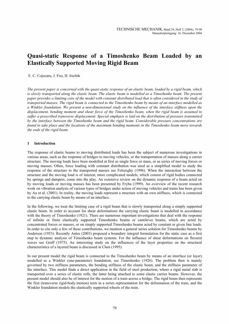
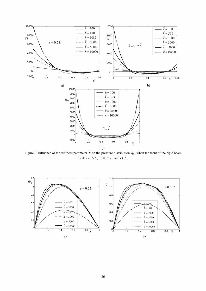
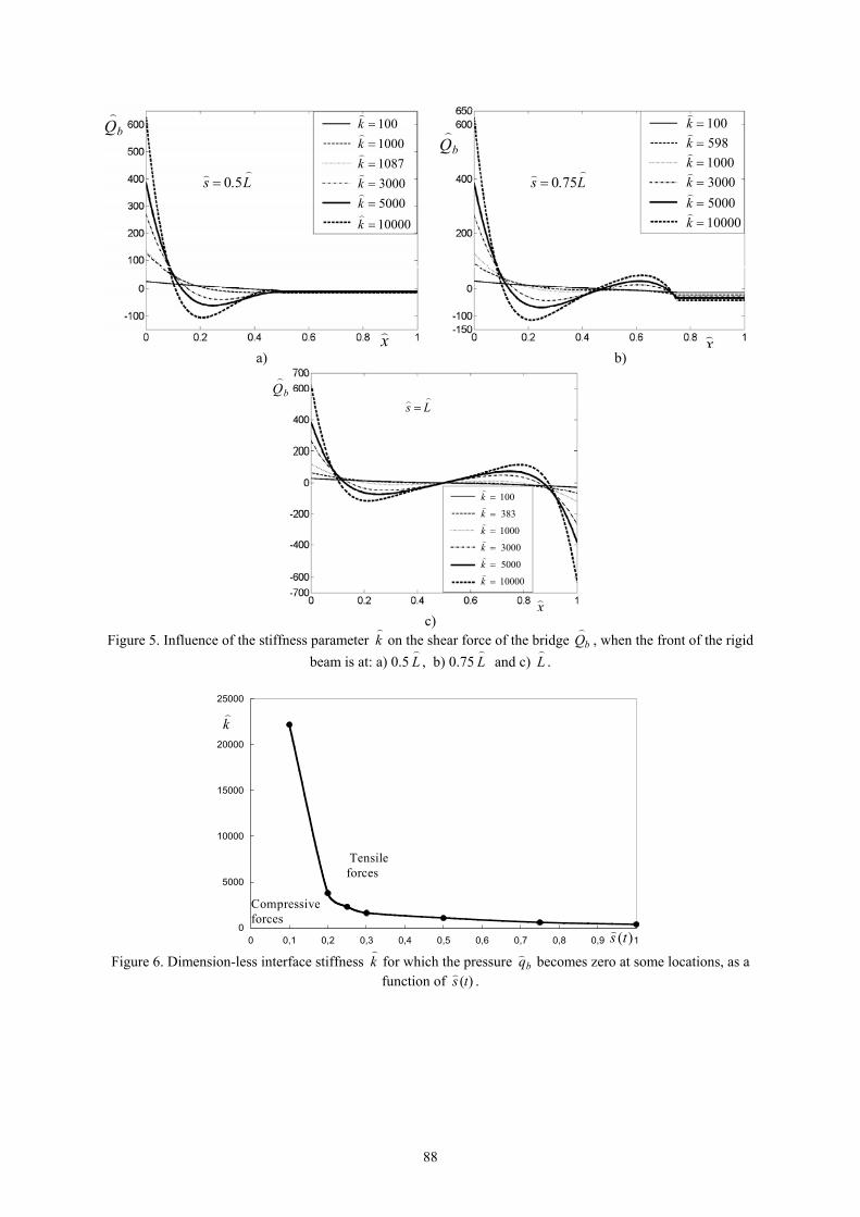
where kt is the correspondent uniform distributed stiffness, L is the length of the elastic beam and N is the finite elements number. For the elastic beam we used the material properties of isotropic steel, defined by the Young's modulus, E, and the Poisson's ratio, ν, the shear modulus being given by G=E/2(1+ν). Thus, a linear static Finite Element analysis was performed, where we prescribed boundary conditions for the bridge at both ends, and for the rigid beam at the rigid body reference node. To verify the validity of the symbolic results we made the same analysis with various numbers of elements and studied the convergence of the deflection and bending moments. 5 Numerical Results 5.1 Symbolic Computation In order to illustrate the influence of the interface linear stiffness upon the pressure distribution between bridge and train, we performed a series of symbolic computations as prescribed above. In all of these computations, the non-dimensional shear coefficient was set to α = 0.005091. This value e.g. corresponds to an bridge structure of 100 m span, consisting of a 7.5×7.5 m box-girder with Ib = 74.65 m4, Ab = 8.64 m2 and γ = 0.44. The material is steel with Young's modulus Eb = 2.1×1011 N/m2, shear modulus Gb = 8.1×1010 N/m2. With the above values one obtains Bb = 1.5676×1013 Nm2, Sb = 3.0793×1011 N. These values were also used in the Finite Element computations. We considered a unit non-dimensional rigid beam's displacement in vertical direction,

) w t = 1, such that the train is displaced towards the bridge. We determined the dimensionless pressure distribution between rigid beam and the bridge

) q b , the dimensionless deflection ) w b , the dimensionless bending moment

) M b and the dimensionless

shear-forces. These computations were performed for five values of the non-dimensional interface stiffness ) k =

100, 1000, 3000, 5000, 10000, and for three locations of the front of the train, ) s (t) = 0.5

) L , 0.75

) L and

) L . The

results are plotted in Figures 2-5. For some location of the train front, we furthermore determinate the non-dimensional interface stiffness

) k for which the minimum of the pressure distribution is zero, that means that the

deflection of the bridge on the respective locations becomes equal to the train displacement, ) w b = ) w t = 1. The

corresponding interface stiffness-values ) k for zero

) q b are depicted in Figure 6 as a function of the front of the rigid beam,

) s (t) . For higher interface stiffness ratios, regions with tensile forces transmitted by the interface take place.

86

) q b

) x

) k = 100) k = 1000) k = 1087) k = 3000) k = 5000) k = 10000

) s = 0.5

) L

) q b

) x

) k = 100) k = 598) k = 1000) k = 3000) k = 5000) k = 10000

) s = 0.75

) L

a) b)

) q b

) x

) k = 100) k = 383) k = 1000) k = 3000) k = 5000) k = 10000

) s =

) L

c)

Figure 2. Influence of the stiffness parameter ) k on the pressure distribution

) q b , when the front of the rigid beam is at: a) 0.5

) L , b) 0.75

) L and c)

) L .

) w b

) x

10000

5000

3000

1087

1000

100

=

=

=

=

=

=

k

k

k

k

k

k

)

)

)

)

)

)

) s = 0.5

) L

) w b

) x

10000

5000

3000

1000

598

100

=

=

=

=

=

=

k

k

k

k

k

k

)

)

)

)

)

)

) s = 0.75

) L

a) b)

87

) w b

) x

) k = 100) k = 383) k = 1000) k = 3000) k = 5000) k = 10000

) s =

) L

c)

Figure 3. Influence of the stiffness parameter ) k on the bridge deflection

) w b , when the front of the rigid beam is at: a) 0.5

) L , b) 0.75

) L and c)

) L .

) M b

) x

) k = 100) k = 1000) k = 1087) k = 3000) k = 5000) k = 10000

) s = 0.5

) L

) M b

) x

) k = 100) k = 598) k = 1000) k = 3000) k = 5000) k = 10000

) s = 0.75

) L

a) b)

) M b

) x

) k = 100) k = 383) k = 1000) k = 3000) k = 5000) k = 10000

) s =

) L

c)

Figure 4. Influence of the stiffness parameter ) k on the bending moment of the bridge

) M b , when the front of the

rigid beam is at: a) 0.5 ) L , b) 0.75

) L and c)

) L .

88

) Q b

) x

) k = 100) k = 1000) k = 1087) k = 3000) k = 5000) k = 10000

) s = 0.5

) L

) Q b

) x

) k = 100) k = 598) k = 1000) k = 3000) k = 5000) k = 10000

) s = 0.75

) L

a) b)

) Q b

) x

) k = 100) k = 383) k = 1000) k = 3000) k = 5000) k = 10000

) s =

) L

c)

Figure 5. Influence of the stiffness parameter ) k on the shear force of the bridge

) Q b , when the front of the rigid

beam is at: a) 0.5 ) L , b) 0.75

) L and c)

) L .

0

5000

10000

15000

20000

25000

0 0,1 0,2 0,3 0,4 0,5 0,6 0,7 0,8 0,9 1

Tensile forces

Compressive forces

)(ts)

) k

Figure 6. Dimension-less interface stiffness

) k for which the pressure

) q b becomes zero at some locations, as a function of

) s (t) .

89

5.2 FEM Analysis For the BOX cross-section of the element B22, the dimensions and material properties given above were used, Bb = 1.5676×1013 Nm2, Sb = 3.0793×1011 N. The uncompressed length of the springs was 0.5 m. The displacement of the rigid beam was prescribed by applying an vertical displacement of 0.25 m at the rigid body reference node. Within the framework of the dimensional Finite Element analysis, excellent agreement with the symbolic computations was found. Exemplary, Figure 7 shows a convergence study for the deflection and bending moment at the mid-span of the fully loaded bridge, using a spring stiffness which corresponds to k

) =

5000. The Finite-Element results converge to the result of the symbolic computation with an increasing number of elements, where the speed of convergence depends on the discrete model of the spring stiffness, see relations from (28).

1,07763

1,07754(Maple )

1,07744

1,07754

1,0760

1,0765

1,0770

1,0775

1,0780

1,0785

1,0790

50 100 150 200 250 300 350 400 450 500 550 600

Number of Elements

Deflection with Abaqus kFEM=kt L/N+1Deflection with Maple7Deflection with Abaqus kFEM=kt L/N-1Deflection with Abaqus kFEM=kt L/N

Def

lect

ion 2,46498

2,46314

2,45270

2,45884

2,30

2,35

2,40

2,45

2,50

2,55

2,60

50 100 150 200 250 300 350 400 450 500 550 600

Number of Elements

Bending Moment with Abaqus kFEM=kt L/N+1Bending Moment with Maple7Bending Moment with Abaqus kFEM=kt L/N-1Bending Moment with Abaqus kFEM=kt L/N

Ben

ding

Mom

ent

a) b)

Figure 7. The convergence of the deflection and bending moment as a function of finite elements number and spring stiffness.

6 Conclusions As can be seen from Figure 2, considerable pressure concentrations take place at the ends of region covered by the rigid beam. These pressure concentrations increase with increasing dimensionless stiffness parameters

) k .

Depending on the location of the front of the train, the pressure distributions become zero somewhere inside the covered (left) region of the bridge for a critical value of

) k , see Figure 6. For larger values of

) k , regions with

tensile (negative) interface forces take place, and the pressure concentrations in the compressive regions at the front of the rigid beam and at the left end of the bridge become more and more pronounced. With an increasing ) k , the distributions of deflection, bending moment and shear-force deviate increasingly from their distributions known for the case of a uniform distributed load, see Figures 3-5. The rigid beam then tends to lift off from the bridge. It was the scope of the present paper to study this effect in some detail, and to provide corresponding information for the practical treatment of this problem. The present study refers to the linear case, in which the Winkler foundation is able to transmit tensile forces. When the latter can not be transmitted, a non-linear treatment of the resulting contact-problem would be necessary. In the present case, we were interested in using the power of linear algebra in combination with symbolic computation to determine the behaviour in case the interface can transmit compressive as well as tensile forces. Our study demonstrates that the space-wise constant line loads, often used in order to model the pressure of a mass moving along a bridge, represent an idealisation that does not lay on the safe side.

Acknowledgements

The support of the authors E. Cojocaru and H. Irschik by the FWF-Austrian Science Fund within the project P14866, "Vibrations of bridge without conservation of mass", is gratefully acknowledged.

90

References ABAQUS/Standard, Theory Manual, Version 6.2, Hibbit, Karlsson &Sorensen, Inc. Anderson, R.A.: Flexural vibrations in uniform beams according to the Timoshenko theory, J. of Applied

Mechanics, 20, 4, (1953), 504-510. Antes, H.: Fundamental solution and integral equations for Timoshenko beams, Computers & Structures, 81,

(2003), 383-396. Au, F.T.K., Cheng, Y.S., Cheung, Y.K. : Vibration analysis of bridges under moving vehicles and trains: an

overview, John Wiley & Sons, Prog. Struct. Engng. Mater., 3, 3, (2001), 299-304. Baker,W.E., Westine,P.S., Dodge,F.T.: Similarity methods in engineering dynamics. Theory and Practice of

Scale Modelling, Revised Edition, Elsevier Science, Amsterdam, (1991). Chen, Y.H., Sheu, J.T.: Beam on viscoelastic foundation and layered beam, Journal of Engineering Mechanics,

ASCE, 121, 2, (1995), 340-344. Felszeghy, S.F.: The Timoshenko Beam on an Elastic Foundation and Subject to a Moving Step Load, Part1:

Steady-State Response, Journal of Vibration and Acoustics, 118, (1996), 277-284. Felszeghy, S.F.: The Timoshenko Beam on an Elastic Foundation and Subject to a Moving Step Load, Part2:

Transient Response, Journal of Vibration and Acoustics, 118, (1996), 285-291. Fryba, L.: Vibration of solids and structures under moving loads, London, Thomas Telford, 1999. Graff, K.F.: Wave motion in elastic solids, London, Oxford University Press, (1975), 180-195. Knothe, K.: Gleisdynamik, Ernst&Sohn, Berlin, (2001). Luenberger, D. G.: Introduction to Dynamic Systems, John Wiley & Sons, (1979). Maple On-line Manual - Version 7, (2001). Timoshenko, S.: On the correction for shear of the differential equation for transverse vibrations of prismatic

bars, Phil. Mag., 41, (1921), 744 – 746. Timoshenko, S.: Method of analysis of statical and dynamical stresses in rail, Proc. second Int. Congress for

Appl. Mech., Zürich, (1926), 407–418. Ziegler,F.: Mechanics of Solids and Fluids, Springer-Verlag, New York, Inc., (1991). _________________________________________________________________________________________ Address: DI Dr. E. Cojocaru, o.Univ.Prof.DI Dr.techn. H. Irschik, Department of Technical Mechanics, Institute of Mechanics and Machine Design, Johannes-Kepler University, Altenbergerstrasse 69, A-4040 Linz, Austria. e-mail:cojocaru@mechatronik.uni-linz.ac.at and irschik@mechatronik.uni-linz.ac.at J. Foo, Research student, on leave from Department of Mechanical Engineering, University of Alberta, 114 Street-8a Avenue, Edmonton, Alberta T6G 2M7, Canada.