Embed Size (px)
Citation preview

Fluid Mechanics 2019; 5(2): 39-71
http://www.sciencepublishinggroup.com/j/fm
doi: 10.11648/j.fm.20190502.12
ISSN: 2575-1808 (Print); ISSN: 2575-1816 (Online)
Quinn’s Law of Fluid Dynamics Pressure-driven Fluid Flow Through Closed Conduits
Hubert Michael Quinn
Department of Research and Development, the Wrangler Group LLC, Brighton, USA
Email address:
To cite this article: Hubert M. Quinn. Quinn’s Law of Fluid Dynamics Pressure-driven Fluid Flow Through Closed Conduits. Fluid Mechanics.
Vol. 5, No. 2, 2019, pp. 39-71. doi: 10.11648/j.fm.20190502.12
Received: October 12, 2019; Accepted: December 11, 2019; Published: January 6, 2020
Abstract: In this paper we develop from first principles a unique law pertaining to the flow of fluids through closed
conduits. This law, which we call “Quinn’s Law”, may be described as follows: When fluids are forced to flow through closed
conduits under the driving force of a pressure gradient, there is a linear relationship between the fluid-drag normalized
dimensionless pressure gradient, PQ, and the normalized dimensionless fluid current, CQ. The relationship is expressed
mathematically as: PQ=k1 +k2CQ. This linear relationship remains the same whether the conduit is filled with or devoid of solid
obstacles. The law differentiates, however, between a packed and an empty conduit by virtue of the tortuosity of the fluid path,
which is seamlessly accommodated within the normalization framework of the law itself. When movement of the fluid is very
close to being at rest, i.e., very slow, this relationship has the unique minimum constant value of k1, and as the fluid
acceleration increases, it varies with a slope of k2 as a function of normalized fluid current. Quinn’s Law is validated herein by
applying it to the data from published classical studies of measured permeability in both packed and empty conduits, as well as
to the data generated by home grown experiments performed in the author’s own laboratory.
Keywords: Closed Conduits, Conduit Permeability, Friction Factor, Wall Effect, Boundary Layer, Turbulent, Flow Profile,
Chaos
1. Introduction
The history of attempts to quantify a relationship between
fluid flow in closed conduits (whether it be in a packed
conduit or in an empty conduit) and the relevant variables
governing that relationship dates back at least to the work of
Darcy in 1856 [1]. Since that time, a host of models have
been proposed with their accompanying array of equations,
each of which has its own limitations and restrictions [2].
Accordingly, the scientific literature is replete with reports of
experimental results aimed at trying to resolve the many
discrepancies which litter the fluid dynamics landscape [3].
In fact, this field of study is in such disarray that there is no
currently accepted theory of fluid dynamics from which one
could derive an analytical solution to the supposed governing
equation of fluid dynamics, the Navier-Stokes equation [4].
This author has devoted his entire career to doing fluid
flow measurements, predominantly in packed beds relating to
the field of HPLC (High Pressure Liquid Chromatography)
[5, 6, 7, 8, 9, 10, 11, 12.]. Rather than nibbling at the fringes
of this complicated field of study by trying to manipulate one
of the currently accepted theories, a completely different
approach was developed. The subsequent model, which we
refer to as the Quinn Fluid Flow Model (QFFM) took
approximately 20 years to formulate, was developed from
first principles, and is different from any other model
currently extant. Most importantly, it is a universal theory
which applies to all fluid flow embodiments, regardless of
whether they contain particles and regardless of the regime of
flow in which they are operated. Moreover, it has been
validated by testing it against a host of generally accepted
experimental data reported in the literature, as well as this
author’s own measurements.
The dimensional manifestation of the QFFM is a complex
equation containing many independent and dependent
variables and is the properly formatted version of the
continuity equation for fluid flow in closed conduits. On the
other hand, there is a dimensionless manifestation of the
QFFM, which we refer to as Quinn’s Law, which is a simple
linear relationship between the reduced pressure gradient and
Fluid Mechanics 2019; 5(2): 39-71 40
the reduced fluid flow current in a closed conduit. In contrast
to the complicated alternatives that conventional theories of
fluid dynamics have to offer, Quinn’s Law is very simple. It
has just two variable parameters. More importantly, and in
contrast to conventional theories, it is valid over the entire
range of the fluid flow regime, providing analytical solutions
in laminar, transitional and fully turbulent ranges of fluid
flow.
This author’s development of the QFFM was born of the
frustration experienced in trying to reconcile experimental
data and textbook teachings relative to packed/empty conduit
permeability. For instance, the chromatographic literature
abounds with erroneous teachings: incorrect use of velocity
frames [13]; the notion that the particle size is defined by
permeability (14); violations of Continuity Laws [15, 16,
17.]; self-serving validations [18]. Likewise, the engineering
literature is littered with similar errors: misapplication of
porosity function [19]; erroneous derivation of the viscous
constant [20]; “blind leading the blind” syndrome [21];
mathematicians using computers to produce mind-numbing
computations, which purport to explain equations that have
no connection to fluid flow parameters in the first place [22];
contradictory statements of facts [23]; etc.; etc. Moreover,
both disciplines are especially guilty of neglecting the role of
kinetic considerations in favor of focusing too much on the
less complex laminar flow regime.
2. Methods
In order to underscore the importance of achieving a
comprehensive understanding of the physics underlying our
theoretical development, rather than just the mathematical
framework, we want to introduce upfront the important novel
concepts which are part of the development of our solution to
the problem. In this way, we hope the reader will be focused
more on where these concepts fit into the overall
comprehensive understanding, rather than becoming
embroiled in the mathematics, which, after all, is simply the
gravel of which the roadway is made, and is not a critical
component to a discussion of what is the destination.
2.1.1. Q - hypothetical Particles
This idea is a very simple one. It is a way of subdividing
the free space in an empty conduit, using the same
mathematics that we use to assign free space to solid particles
in a packed conduit. We accomplish this by extending the
existing framework of particle porosity for packed conduits
containing solid particles to accommodate particles of free
space (no solid skeleton) in an empty conduit. The resultant
framework is a universe of two mathematical half-planes,
each of which is the mirror image of the other. Of particular
importance in this theoretical development, however, is that
we manage to avoid the point of discontinuity which would
otherwise arise as a consequence of the theory at the axis of
symmetry between the two mathematical half-planes, since
this would cause the mathematics and, consequently, the
entire logic to implode at this location. We accomplish this
task by only using the absolute value of the particle fraction
[abs (1-ε0)] function, which is always finite, in our definition
of the Hypothetical Q Channel (HQC) diameter, dc, which
forms the basis of the QFFM. In other words, we only use
that portion of the theory which is valid in the real world. In
addition, we are careful to manage our mathematical
framework to incorporate the Conservation Laws into our
HQC by a mechanism which reconciles particle diameter, dp,
and conduit external porosity, ε0.
2.1.2. rh-the Fluid Drag Normalization Coefficient
The concept underlying this parameter is, arguably, the
most important element of the entire QFFM theory. It is the
exchange rate necessary to create a common “currency”
between viscous and kinetic considerations dictated by the
Laws of Nature. We use the value of the ratio of surface area
to cross-sectional area of a spherical particle, rh, i.e., 4, to
define our control volume, (4πrh3/3=268), making this value
the common denominator which connects the control
volume, surface area, cross sectional area and fluid drag.
Accordingly, in our permeability model, this common
denominator takes on the dual role of (a) being the radius of
the obstacle responsible for the fluid friction due to viscous
considerations, and, (b) at the same time, represents the
hydraulic radius of the flow channel responsible for the fluid
friction due to kinetic considerations. We exploit this feature
in our theory by providing a mechanism for normalizing fluid
resistance by either (1) surface area contact (k1=4πrh2/3=67),
or, (2) reciprocal channel circumference (k2=1/ (2πrh)=1/25).
2.1.3. δ-the Porosity Normalization Coefficient This parameter represents one of the cornerstones of our
theory which allows us to accommodate both packed and
empty conduits. It is a specific property of the flow
embodiment under study. For instance, the same packed
conduit with x number of particles will have a different value
for δ, than the same conduit packed with y number of the
same particles. Thus, a packed and an empty conduit will
also have different δ values. Our δ parameter establishes in
our theory (and is confirmed by our pressure drop
measurements) that the pressure drop in the kinetic term of
the permeability equation is inversely proportional to the 6th
power of the conduit external porosity. By combining our
parameter δ with the modified Reynolds number, Rem, we
create a unique grouping of terms, our QN parameter, which
we term fluid current. This parameter is the engine that
drives the fluid velocity profile and, accordingly, reconciles
all forms of flow.
2.1.4. γ-the Architectural Normalization Coefficient
This parameter is a rather obvious development to anyone
who has experience in building physical structures from
scratch, such as a house or barn or wall, all of which are
made of building blocks of wood/bricks/stones and,
accordingly, forms the basis for one’s thinking when one
builds a packed conduit from building blocks of particles
(stones) within a fixed volume of free space, i.e. a conduit.
41 Hubert Michael Quinn: Quinn’s Law of Fluid Dynamics Pressure-driven Fluid Flow Through Closed Conduits
2.1.5. λ-the Wall Effect Normalization Coefficient of Fluid
Current
This parameter is another cornerstone in our framework
which aligns the physics of a packed and empty conduit, but
only manifests in the kinetic term. It is also a specific
property of the flow embodiment under study, and only
changes as a function of the specific wall effect of a given
packed conduit. In this case, however, the effect of the wall is
transferred to the motion of the fluid, which is why we
describe it as a component of fluid current. The rationale
behind this parameter is fairly well documented in the main
body of our paper, wherein we took advantage of Prandtl’s
concept of the boundary layer in formulating our definition
of the primary wall effect [24].
2.1.6. τ-the Tortuosity Normalization Coefficient
We believe that tortuosity is primarily a function of
channel architecture normalized for conduit external porosity.
Accordingly, we have defined this parameter as another
normalization coefficient which, again, only manifests in the
kinetic term of the permeability equation. It compensates for
the different flow paths which are generated within different
packed conduits, as well as compensating for the unique flow
path generated within all empty conduits.
2.1.7. The Harmonic Oscillator
Finally, everything comes together in our notion that fluid
flow in closed conduits, whether packed with solid particles
or empty, is a form of harmonic motion. Intuition tells us that
we ought to imagine that the fluid going through a packed
bed has to somehow double back upon itself. This idea led to
the concept of Simple Harmonic Motion (SHM). Once
having understood that SHM was the operating principle
governing fluid flow in closed conduits, the connection to
uniform circular motion became obvious. This led to the
realization that when the speed of the fluid at the wall is zero,
the velocity is not zero because the fluid is changing
direction simultaneously. This was enough to establish the
viscous friction factor as the underlying concept behind the
harmonic oscillator algorithm. Once having done this, it was
relatively easy to figure out what parameter was what, in the
fluid motion, and make a one-to-one correspondence between
the dimensionless fluid viscous friction factor parameters and
the dimensional simple harmonic motion parameters, which,
incidentally, is the reason why the particular units of measure
in the SHM can be arbitrary, as long as they are self-
consistent. More accurately stated, we incorporate the
framework of damped-SHM to accommodate the impact of
conduit wall friction and fluid internal friction, using both as
damping coefficients on the overall motion of the fluid.
The concept of “fluid chaos”, which permeates
conventional wisdom, is rejected in our theory. The best way
to think about it is to imagine oneself as a hunter in the
mountains. The deer, which is the focus of our hunt, is
perfectly camouflaged against the background of the hillside.
Thus, the deer is invisible to the hunter, despite the fact that
the deer’s body is located in free space in all three
dimensions, i.e., it has location coordinates in the x, y and z
planes. The reason why the deer is invisible to the hunter is
that, relative to the hillside background, the hunter cannot
differentiate between the deer and the underbrush. It is only
when the deer changes its positional coordinates relative to
the hill in the background that the hunter can see it i.e., when
the deer starts running. Moreover, because the movement of
the deer is not restricted in terms of free space on the
mountainside, his “movement profile” can be erratic, uniform
in a straight line (if he follows a road, for instance), or
combinations of the above, all driven by the whim of the
deer’s instincts. However, it is never chaotic or
unpredictable, in a scientific context, that is.
In our Hypothetical Q Channel model, the fluid is
equivalent to the deer, i.e., it has positional coordinates in all
three planes, but the fluid flow profile cannot be
distinguished from the background of the channel because its
positional coordinates are indistinguishable relative to the
conduit wall or conduit center line. It is only when we view
the fluid through the “scope” of the QN parameter (4th
dimension), that its positional coordinates are changed
relative to the background conduit wall/center line. In
addition, when viewing the fluid profile through the QN
scope, the QN crosshairs must be spaced closely enough
together, relative to the size of T, the time constant of the
fluid motion, to generate a comprehensive image of the flow
profile, just as the crosshairs in the hunter’s telescopic sight
must be adjusted, commensurate with the overall size of the
deer.
Additionally, and in contrast to the movement of the deer,
the fluid movement in our HQC is restricted in free space
because of its driving force, i.e., the pressure drop (∆P).
Furthermore, when we normalize the pressure drop for the
length of the conduit, L, i.e., the pressure gradient (∆P/L), we
restrict the movement of the fluid even further, i.e., to just the
cross-section of the HQC. Thus, as the fluid moves over the
cross-section, its current is influenced by the walls of the
conduit, i.e., wall friction. Because of internal fluid friction,
as its speed increases, the fluid flow profile loses its “arc of
motion” and, ultimately, simply moves back and forth over
the cross-section in a virtual straight line, i.e., “plug flow”.
Thus, cross-channel mixing is greatly enhanced by
convection which is driven by the kinetic term in the
permeability equation.
The Hypothetical Q Channel, of course, does not exist in
the real world. However, the model allows us to imagine the
fluid moving through the conduit and when we do, what we
see is not disorganized or chaotic motion, but a structural
pattern characterized by SHM, regardless of Reynolds
number or any conduit or particle parameter. Accordingly, we
suggest that “fluid chaos” is in the eye/mind of the beholder.
2.1.8. Conventional Permeability Equations
Finally, having started at the beginning of our development
with fundamental definitions, we make our way
systematically through the governing equations, in order to
Fluid Mechanics 2019; 5(2): 39-71 42
arrive at the equation most useful to the practitioner of
permeability. In so doing, we are mindful to connect our
QFFM to the conventional Poiseuille and Ergun flow models,
albeit through a modified version for terms, which corrects
for the glaring shortcomings of each.
2.2. Fundamentals of the Q Fluid Flow Model (QFFM)
2.2.1. Particle
Let us define an obstacle to be placed within a packed
conduit as a spheroidal particle of nominal diameter dpm and
sphericity Ωp. Then we may write:
dp=dpmΩp (1)
Where, dp=the spherical particle diameter equivalent
Ωp ≤ 1; thus, when Ωp=1, the particle is spherical.
Let the particle have a specific pore volume of Spv, a
skeletal density of ρsk, and a mass of mp.
Let us define other particle characteristics as:
SAp=πdp2 (2)
And
CSAp=
(3)
Where, SAp=particle equivalent surface area; and
CSAp=particle equivalent cross sectional area.
It follows that we may write:
Vdp=
(4)
ρpart=
(5)
Where, Vdp=the volume of a single spherical particle
equivalent; ρpart=the apparent particle density.
Let us define particle porosity as the ratio of free space
within the particle to the total free space occupied by the
particle as a whole, thus:
εp=Spvρpart (6)
Where, εp=the particle porosity.
It follows that:
When, εp=1, the particle is devoid of solid matter, i.e.
contains only free space;
When, εp=0, the particle is made entirely of solid matter,
i.e. the particle is non-porous;
When, 0 ≤ εp < 1, the particle is partially porous, i.e.,
consists of a solid particle skeleton plus internal pores.
2.2.2. Conduit
Let us define a fluid conduit as a right circular cylinder of
length L and diameter D. Then we may write:
Vec=
(7)
Where, Vec= the volume of free space within an empty
conduit.
Let the conduit be packed with np number of particle
equivalents of diameter dp.
It follows that we may write:
Vpart=
(8)
Where, Vpart=the cumulative volume occupied by all the
particle equivalents within a packed conduit.
Let us define as npq, the number of particle equivalents
whose collective volume is equal to the volume of free space
within an empty conduit.
It follows that we may write:
=
=
(9)
Let us define the packed conduit fluidic architecture as:
γ =!"
(10)
Where, γ=the fluidic architectural coefficient for a given
packed conduit.
We now turn to conduit porosities.
Let us define the volume of free space within the packed
conduit which is external to all the particles as Ve; the
volume of free space which is internal to all the particles as
Vi; the volume which is occupied by all the particle skeletons
as Vsk; and Vt as the total volume of free space within the
packed conduit which is devoid of solid matter.
It follows that we may write:
#1 − &'( =!!"
=)*+
(11)
Where, the conduit particle fraction, (1−ε0)=the volume
fraction of the packed conduit occupied by the particles.
&,- =#./0(!
!"= 12
(12)
Where, the conduit skeletal porosity, εsk=the volume
fraction of the packed conduit occupied by the particle
skeletons.
&' =./!!"
=
(13)
Where, the conduit external porosity, ε0=the volume
fraction of the packed conduit external to the particles.
&3 =  − &'( =4
(14)
Where, the conduit internal porosity, εi=the volume
fraction of the packed conduit internal to the particles.
&5 = 1 −#./0(!
!"= &3 + &' (15)
Where, the conduit total porosity, εt=the sum of the
volume fractions external and internal to the particles.
It follows that particle porosity and conduit internal
porosity are related as follows:
43 Hubert Michael Quinn: Quinn’s Law of Fluid Dynamics Pressure-driven Fluid Flow Through Closed Conduits
when εp=0, conduit internal porosity εi=0 and, thus, the
particles are completely solid throughout, i.e., non-porous.
when εp=1, conduit internal porosity εi=(1-ε0) and thus, the
particles are completely devoid of solid matter, i.e., totally
porous.
Additionally, it follows that reconciling the definitions
above for solid matter and lack thereof, i.e., porosity, within a
conduit, [see Eqs. (8) and (11) above], we may now write:
!
= 789:;<#1 − &'( (16)
Equation (16) reconciles the distribution of free space
within the conduit according to the conservation Laws of
Nature, whereby all partial volume fractions of the fluid-
filled packed conduit, whether occupied by solid matter or
fluid, add to unity.
2.2.3. The Conservation Laws Governing Packed Conduits
Thus, the Conservation Laws pertaining to packed
conduits dictate that we may write:
ε0 + εi + εsk=1 (17)
or
εt + εsk=1 (18)
Let us define the packing density of a packed conduit as:
=>9- =?
(19)
Where, ρpack=the packing density of the packed conduit;
Mp=npmp, the total mass of all the particles in a packed
conduit under study.
It follows that we may now write:
ε0=1-ρpack(Spv-1/ρsk) (20)
or
ε0=1- [2npdp3/(3D
2L)] (21)
Accordingly, we may write:
& = 0+/0@./0@
(22)
Substituting for the independently measured components
of εp in Equation (22), gives
AB=>C5 =0+/0@./0@
(23)
It therefore follows that, empirically, we may define a
packed conduit in terms of 4 independent variables (Mp, Vec,
Spv, ρsk) or, alternatively, (np, dp, D, L), in combination with
one dependent variable (ε0), all of which are measureable.
However, if in addition to measuring the independent
variables, one also measures the value of the external
porosity, ε0 (a dependent variable), both sides of Equations
(22) and (23) must be reconciled for any given packed
conduit under study, as dictated by the Conservation Laws
(sometimes referred to as the Laws of Continuity when their
application involves moving entities like the fluid in this
particular application). This dictate from the Laws of
Continuity trumps all measurement techniques, which
generally lack the specificity/accuracy to balance either
equation without the need for further reconciliation or
modification.
Thus, the left hand side of Equation (23) contains
measurements made outside of the packed conduit, i.e.,
independent of the packed conduit under study, whereas the
right hand side of Equation (23) contains measurements
made within the packed conduit under study. Accordingly,
balancing of Equation (23) is always necessary to validate
the accuracy of the reported values for the measured
parameters of the packed conduit under study.
It follows that, in the case of packed conduits which
contain nonporous particles, Equation (23) is equal to zero on
both sides of the equalization sign, thus eliminating the need
to reconcile column porosity and particle porosity.
2.2.4. The Q-Porosity Function (ε)
Let us now collect all the partial porosity definitions in the
QFFM underlying packed conduits which are defined in
terms of particle size equivalents and view them as
dimensionless mathematical functions of np, which we will
designate as Q-Porosity functions. There are a total of 5 such
functions, which we view in the context of the generalized Q-
Porosity function ε.
1. (1-ε0)=np/npq, Equation (11) above.
2. εsk=(1-εp)np/npq, Equation (12) above.
3. ε0=(1-np/npq), Equation (13) above.
4. εi=εp (np/npq), Equation (14) above.
5. εt=1- (1-εp)np/npq, Equation (15) above.
It now becomes obvious that the Q-Porosity functions ε0
and (1-ε0) are independent of the value of the particle
porosity, εp.
Similarly, it is also obvious that the Q-Porosity functions
εi, εsk and εt are dependent on the value of the particle
porosity, εp.
2.3. The Conduit Packing Process
2.3.1. Solid Particles (0 ≤εp <1( Let us now define the conduit packing process in the case
of solid particles (0 ≤ εp < 1( by viewing the role of our
independent variable, np, within the context of the Q-Porosity
function (ε). This is best accomplished by viewing a worked
example on a plot of the dimensionless Q- Porosity function,
ε, versus the number of particle equivalents, np.
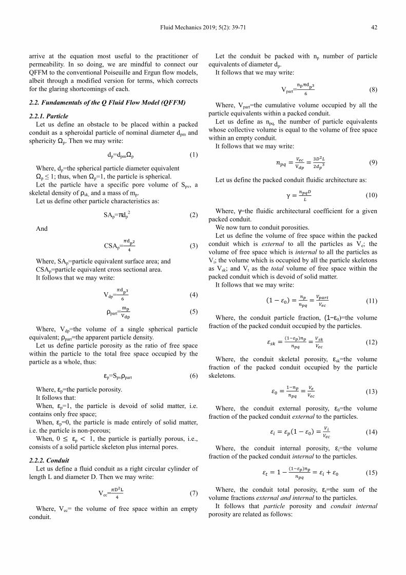
Our chosen worked example consists of 10 micron
particles packed into a conduit of dimensions 10 cm in length
and 0.46 cm in diameter, the details for which are presented
in Figure 1, for the case in which the particles are nonporous
(εp=0).
As shown in Figure 1 below, our empirical packing
process recognizes Kepler’s conjecture regarding the
stacking of solid spheres. Accordingly, the maximum value
of the Q-Porosity function (1-ε0) is approximately 0.74 with
Fluid Mechanics 2019; 5(2): 39-71 44
the corresponding minimum value of approximately 0.26 for
the Q-Porosity function ε0. Kepler’s conjecture is a
consequence of the fact that solid spheres and free space are
mutually exclusive and therefore the maximum value of np
achieved empirically must be less than the value of npq. The
upper limit of the value of np is always npq since it represents
the most particle equivalents, theoretically, that could be
packed into any given conduit under study.
Accordingly, the theoretical domain of the Q-Porosity
function (ε) runs from 0 to npq and the ranges of the function
vary between the values of 0 and 1, as shown in Figure 1.
Figure 1. Q-Porosity Function for Non-Porous Particles (εp=0).
In Figure 1 we only display two of the Q-Porosity
functions, i.e., ε0 and (1-ε0), since they are not influenced by
the particle porosity value, εp, and, in this particular case
(εp=0), εi=0, εt=ε0 and εsk=(1-ε0). Additionally, we note that
these two functions are reciprocal in nature to the extent that
as one increases, the other decreases, all as a function of np.
We now further refine the definition of the entity np to be
that of a vector rather than a scalar quantity and, therefore,
confer upon it a directional component in addition to its
mandatory magnitude component.
Let us now define the packing process of a conduit, using
our example with solid particles, in terms of our
mathematical Q-Porosity functions, as the direction of
increasing positive values of np. Thus, as we move along the
x axis of Figure 1 in the direction of left to right, starting at
the origin of the plot at np=0, the corresponding values on the
y axis represent the changing characteristics of the Q-
Porosity function ε in the filling (packing) process. At the
starting point of np=0, the conduit is devoid of particles
(contains only free space) and at the maximum value of np
achieved in the filling process, the conduit is fully packed.
Accordingly, filling of a “packed” conduit with solid
particles is represented by the increasing positive values of
np, i.e., the motion left to right along the x axis of the plot
starting at the value of np=0 .
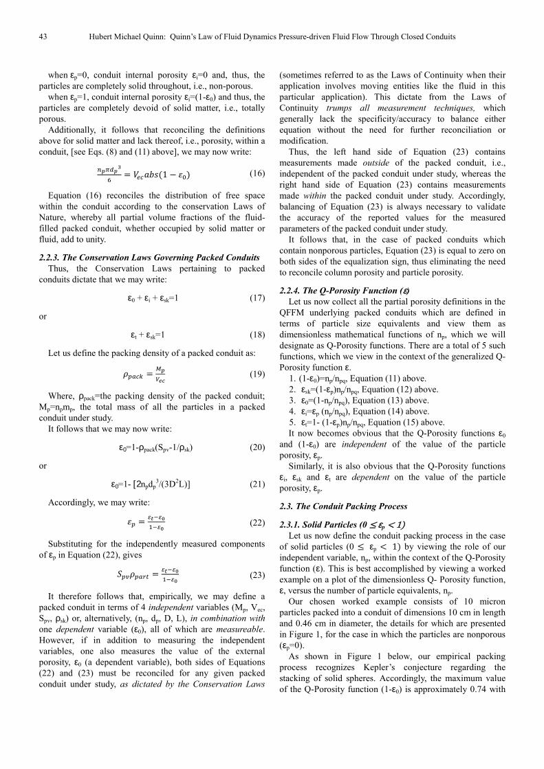
We shall now consider the more complex packing process
in which the particle porosity varies between the values of 0
and 1, i.e., the case of partially porous particles (0 < εp <1).
In our worked example shown in Figure 2, we show as our
example a packed conduit with particles which have a
particle porosity of 0.6 (εp=0.6). Because the porosity
functions of εi, εt and εsk are dependent on the value of εp, we
include these functions in our Figure 2.
As displayed in Figure 2, each of the 5 porosity functions,
ε0, (1-ε0), εi, εt, and εsk have discrete and different values for
all values of np.
Figure 2. Q-Porosity Function for Partially Porous Particles (0 < εp < 1).
45 Hubert Michael Quinn: Quinn’s Law of Fluid Dynamics Pressure-driven Fluid Flow Through Closed Conduits
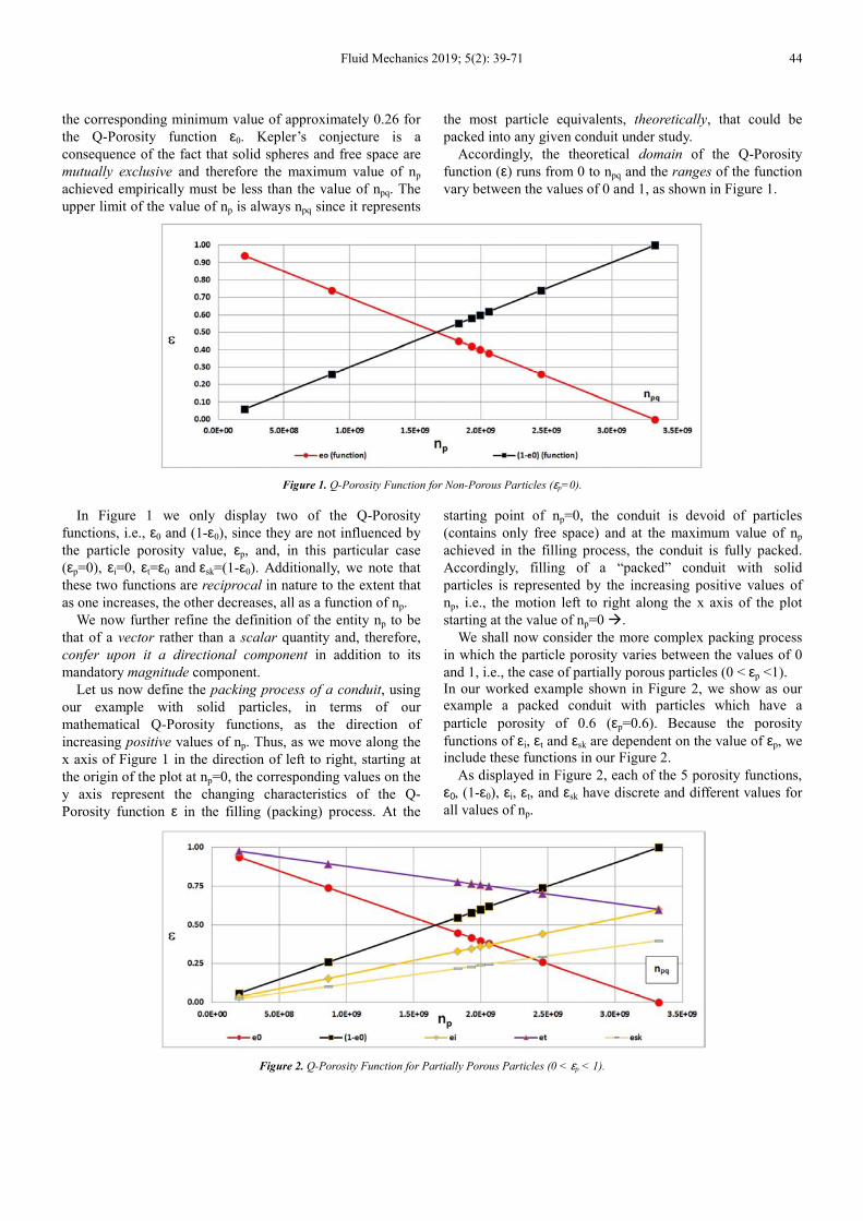
2.3.2. Hypothetical Q-Particles (εp=1( We shall now consider the packing process in the special
case when the particles are fully porous, i.e., they are
completely made of free space (εp=1). This scenario is
presented in Figure 3.
As shown in Figure 3, our packing process for particles
made of free space (εp=1), which we designate as
hypothetical Q-particles, is represented by increasingly
negative values of np. Accordingly, the domain of the Q-
Porosity function runs from 0 to - npq. Similarly, it follows
that the range of the function varies between the values of -1
and 2, as shown in the plot.
Figure 3. Q-Porosity Function for Fully Porous Particles (εp=1).
In this scenario the Q-Porosity functions εt=1 and εsk=0 for
all values of np. The function εi has identical values to the
function (1-ε0) and varies between 0 and -1, whereas the
value of the function ε0 varies between 1 and 2.
Let us now define the directional component of packing a
conduit with hypothetical Q-particles in terms of our
mathematical Q-Porosity functions. As we move along the x
axis of Figure 3 in the direction of right to left, starting at the
origin of the plot at np=0, the corresponding values on the y
axis represent the changing characteristics of the Q-Porosity
function ε in the filling (packing) process. This direction of
filling is the opposite of that for solid particles. At the
starting point of np=0, we consider the conduit to be devoid
of all particles (including particles of free space) and at the
maximum value of np=- npq achieved in the filling process,
the conduit is fully packed with particles of free space
(hypothetical Q-particles). Accordingly, filling of a “packed”
conduit with hypothetical Q-particles is represented by
increasing negative values of np, i.e., the motion right to left
along the x axis of the plot starting at np=0 .
It follows that in the case of hypothetical Q-particles
which are made of free space, Kepler’s conjecture does not
apply, since particles of free space are mutually inclusive
with free space, i.e., they are free space. Accordingly, the
maximum value of np achieved empirically is -npq, which
corresponds to the conduit being filled with free space, and is
also the upper theoretical limit of np in these circumstances.
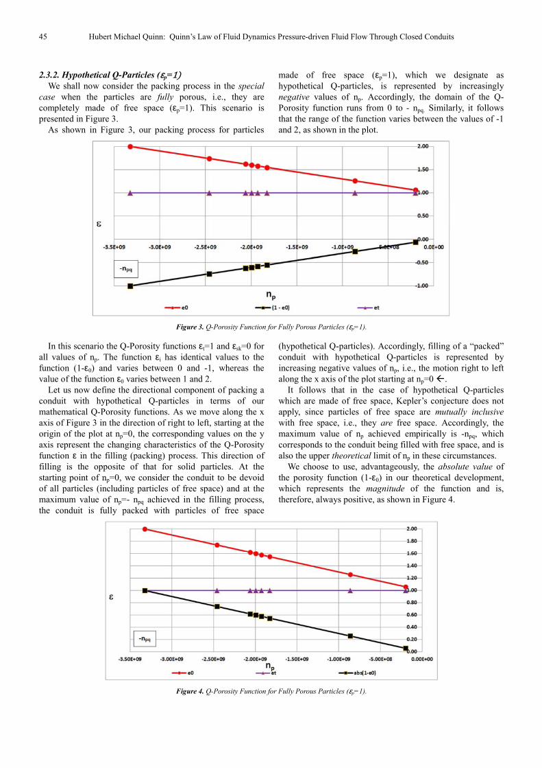
We choose to use, advantageously, the absolute value of
the porosity function (1-ε0) in our theoretical development,
which represents the magnitude of the function and is,
therefore, always positive, as shown in Figure 4.
Figure 4. Q-Porosity Function for Fully Porous Particles (εp=1).
Fluid Mechanics 2019; 5(2): 39-71 46
Accordingly, as shown in Figure 4, the ranges of all Q-
Porosity functions of interest in this special case have
positive magnitudes, and vary between the values of 0 and 2.
2.3.3. The Packed Conduit Hypothetical Q Channel
Defined
Let us define a hypothetical cylindrical fluid channel
within a packed conduit, which we shall call the hypothetical
Q channel (HQC), whose characteristic dimensions are
defined as:
D9 =
>E,#./0@(=
>E,#!/!"(
(24)
Where, dc=the diameter of the HQC.
It follows that we may write [see Eqs. (7) and (14)]:
79 = 789&5 =!"
0+
(25)
Where, vc=the volume of the HQC.
It follows that we may also write:
:9 =
=
!"
! (26)
Where, ac=the cross sectional area of the HQC.
Similarly, we may write:
G9 =>
=!0+
!" (27)
Where, lc=the length of the HQC.
Let us define the Unit Hypothetical Q Channel as a special
case of the more general HQC. It is defined as a conduit
filled with hypothetical Q-particles having two fixed
boundary conditions: (1), dp=D and (2), np=-npq.
It follows that, since the function ε0=2 when np=-npq, the
function abs (1-ε0)=1=εt.
Accordingly, any “empty” conduit/capillary is represented
in the QFFM by what we now term the Unit HQC since, by
definition, its Q-Porosity functions of [abs (1-ε0)] and εt are
unity, as shown above in Figure 4 for our worked example.
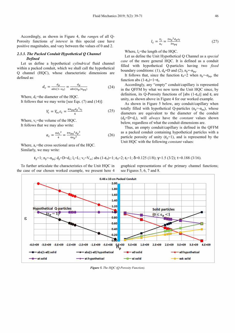
As shown in Figure 5 below, any conduit/capillary when
totally filled with hypothetical Q-particles (np=-npq), whose
diameters are equivalent to the diameter of the conduit
(dp=D=dc), will always have the constant values shown
below, regardless of what the conduit dimensions are.
Thus, an empty conduit/capillary is defined in the QFFM
as a packed conduit containing hypothetical particles with a
particle porosity of unity (εp=1), and is represented by the
Unit HQC with the following constant values:
εp=1; np=-npq; dp=D=dc; lc=L; vc=Vec; abs (1-ε0)=1; ε0=2; εt=1; δ=0.125 (1/8); γ=1.5 (3/2); τ=0.188 (3/16).
To further articulate the characteristics of the Unit HQC in
the case of our chosen worked example, we present here 4
graphical representations of the primary channel functions;
see Figures 5, 6, 7 and 8.
Figure 5. The HQC (Q-Porosity Function).
47 Hubert Michael Quinn: Quinn’s Law of Fluid Dynamics Pressure-driven Fluid Flow Through Closed Conduits
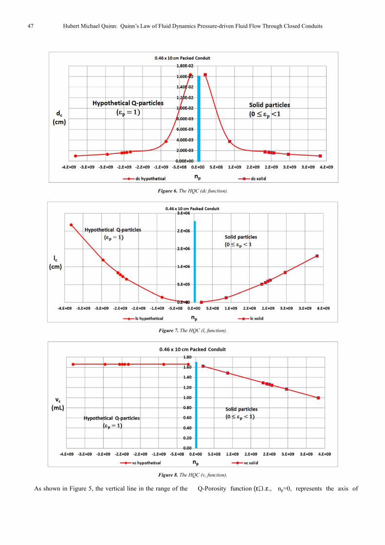
Figure 6. The HQC (dc function).
Figure 7. The HQC (lc function).
Figure 8. The HQC (vc function).
As shown in Figure 5, the vertical line in the range of the Q-Porosity function (ε), ι.ε., np=0, represents the axis of
Fluid Mechanics 2019; 5(2): 39-71 48
symmetry between the half-plane Q-Porosity function for
solid particles, on the one hand (right hand side half-plane),
and hypothetical Q particles, on the other hand (left hand side
half-plane). Note that the Q-Porosity functions are
discontinuous at the value of np=0, but are continuous at all
other values of np, i.e., -npq ≤np <0; 0 <np ≤npq.
It follows that, as shown in Figure 6, the HQC function dc
is correspondingly discontinuous at the value of np=0, since
at this precise value the diameter of the HQC tends to
infinity. Thus, in the QFFM, the “infinite diameter packed
conduit” is prohibited by hypothesis.
Finally, it follows that, as shown in Figure 7, the HQC
function lc is zero at the value of np=0. In addition, the value
of lc is always greater for values of np less than zero, than for
values of np greater than zero, a consequence of a value for
external porosity in excess of unity, in this half-plane of the
function.
Similarly, it follows that, as shown in Figure 8, the HQC
function vc is correspondingly discontinuous at the value of
np=0, since at this precise value, the volume of the HQC is
undefined, but at all values of np less than zero, its volume is
a constant positive value and at all values of np greater than
zero, it has a variable positive value.
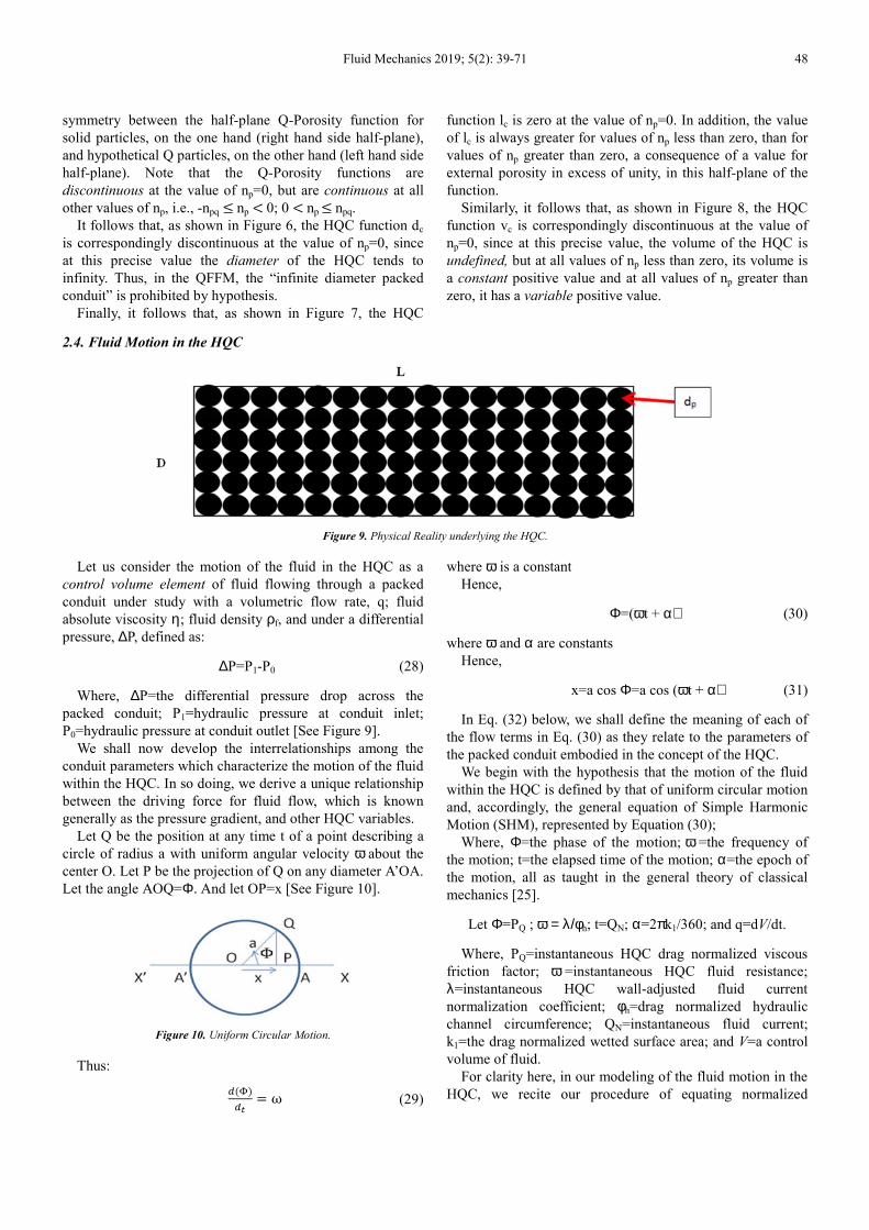
2.4. Fluid Motion in the HQC
Figure 9. Physical Reality underlying the HQC.
Let us consider the motion of the fluid in the HQC as a
control volume element of fluid flowing through a packed
conduit under study with a volumetric flow rate, q; fluid
absolute viscosity η; fluid density ρf, and under a differential
pressure, ∆P, defined as:
∆P=P1-P0 (28)
Where, ∆P=the differential pressure drop across the
packed conduit; P1=hydraulic pressure at conduit inlet;
P0=hydraulic pressure at conduit outlet [See Figure 9].
We shall now develop the interrelationships among the
conduit parameters which characterize the motion of the fluid
within the HQC. In so doing, we derive a unique relationship
between the driving force for fluid flow, which is known
generally as the pressure gradient, and other HQC variables.
Let Q be the position at any time t of a point describing a
circle of radius a with uniform angular velocity ω about the
center O. Let P be the projection of Q on any diameter A’OA.
Let the angle AOQ=Φ. And let OP=x [See Figure 10].
Figure 10. Uniform Circular Motion.
Thus:
#H(
+= ω (29)
where ω is a constant
Hence,
Φ=(ωt + α) (30)
where ω and α are constants
Hence,
x=a cos Φ=a cos (ωt + α) (31)
In Eq. (32) below, we shall define the meaning of each of
the flow terms in Eq. (30) as they relate to the parameters of
the packed conduit embodied in the concept of the HQC.
We begin with the hypothesis that the motion of the fluid
within the HQC is defined by that of uniform circular motion
and, accordingly, the general equation of Simple Harmonic
Motion (SHM), represented by Equation (30);
Where, Φ=the phase of the motion; ω =the frequency of
the motion; t=the elapsed time of the motion; α=the epoch of
the motion, all as taught in the general theory of classical
mechanics [25].
Let Φ=PQ ; ω = λ/φh; t=QN; α=2πk1/360; and q=dV/dt.
Where, PQ=instantaneous HQC drag normalized viscous
friction factor; ω =instantaneous HQC fluid resistance;
λ=instantaneous HQC wall-adjusted fluid current
normalization coefficient; φh=drag normalized hydraulic
channel circumference; QN=instantaneous fluid current;
k1=the drag normalized wetted surface area; and V=a control
volume of fluid.
For clarity here, in our modeling of the fluid motion in the
HQC, we recite our procedure of equating normalized
49 Hubert Michael Quinn: Quinn’s Law of Fluid Dynamics Pressure-driven Fluid Flow Through Closed Conduits
dimensionless parameters related to the HQC to dimensional
parameters in our SHM model. Thus, for instance, the
dimensionless parameter QN of the HQC is equated to the
elapsed time parameter t, of the SHM model, which has the
dimensional units of seconds.
Note also that we have arbitrarily chosen the units of
radians in our definition of the epoch of the motion in the
SHM model, by virtue of the unit conversion (2π/360), which
is the conversion factor between degrees and radians.
Thus, substituting for the terms which define our fluid
motion in the HQC, we may now rewrite Equation (30) as
follows:
PQ=(k1 + λQN/φh) (32)
It follows that we may state that, in the limit as QN tends to
zero, the value of PQ approaches the constant value of k1. We
can express this algebraically as:
JK = L.MNOPQ → 0
Thus, the function PQ is bounded only on one side and
varies from a minimum value of k1 on the low side, when the
fluid is at rest (QN=0), and is unbounded on the high side
(high value of QN).
Let us define a corresponding HQC kinetic friction factor
as:
JT =UVKW
(33)
Where, PK=the instantaneous HQC normalized kinetic
friction factor.
Thus, the function PK is infinite when the fluid is at rest
(QN=0).
Driven by the principle of avoiding non-finite boundaries,
let us define the reciprocal of Equation (33) as:
.
UX= KW
UV= Θ (34)
Where, Θ =the dimensionless permeability of the HQC.
It follows that we may write:
Θ = .
-Z/KW[\/]^ (35)
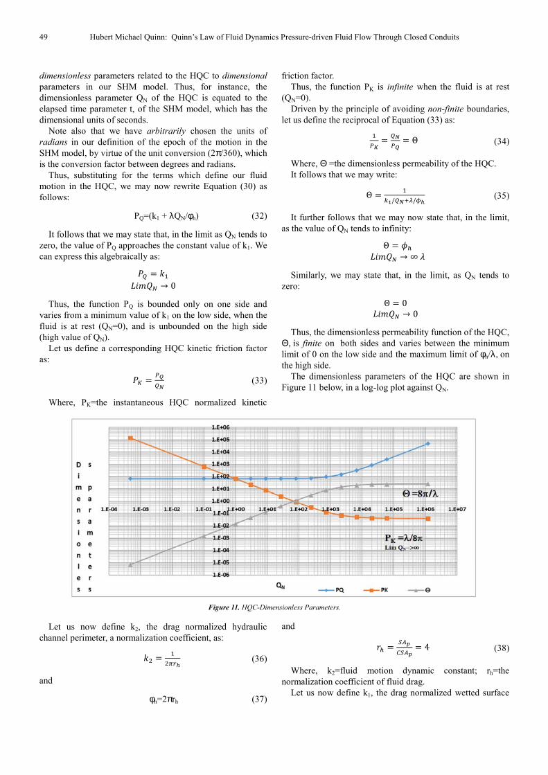
It further follows that we may now state that, in the limit,
as the value of QN tends to infinity:
Θ = _`
MNOPQ → ∞b
Similarly, we may state that, in the limit, as QN tends to
zero:
Θ = 0MNOPQ → 0
Thus, the dimensionless permeability function of the HQC,
Θ, is finite on both sides and varies between the minimum
limit of 0 on the low side and the maximum limit of φh/λ, on
the high side.
The dimensionless parameters of the HQC are shown in
Figure 11 below, in a log-log plot against QN.
Figure 11. HQC-Dimensionless Parameters.
Let us now define k2, the drag normalized hydraulic
channel perimeter, a normalization coefficient, as:
L = .
C^ (36)
and
φh=2πrh (37)
and
c =defde
= 4 (38)
Where, k2=fluid motion dynamic constant; rh=the
normalization coefficient of fluid drag.
Let us now define k1, the drag normalized wetted surface
Fluid Mechanics 2019; 5(2): 39-71 50
area, a normalization coefficient, as:
L. = C^
=
(39)
It follows that we may now rewrite Equation (32) as:
JK =
= \KW
h (40)
Let us define δ, a porosity normalization coefficient, as:
δ = .
0@ (41)
Let us define τ, a tortuosity normalization coefficient, as:
τ=δγ (42)
Let us now define QN, the instantaneous fluid current, a
dimensionless parameter, as:
QN=δRem (43)
Where, Rem=the modified Reynolds number, defined
below in Eqs. (54), (55) and (57). Let us now define λ, the HQC wall-adjusted fluid current
normalization coefficient, as:
λ=(1+WN) (44)
Where, WN=the net wall effect, and is restricted to where 0
≤WN
It follows that we may now rewrite Equation (40) as:
JK =
= j\kl
C^ (45)
Substituting for λ in Equation (45), gives:
JK =
= j#.[mW(kl
C^ (46)
Let us further refine the definition of WN as:
WN=W1 + W2R (47)
Where, W1 = the primary wall effect, defined below;
W2R=the residual secondary wall effect, defined below.
Let us define ω0, the dimensionless resistance of the fluid
in the absence of any wall effect (λ =1), i.e., WN=0, as
follows:
n' = .
∅^ (48)
Let us define β0, the dimensionless fluid/wall boundary
layer in the absence of wall effect (λ=1), i.e., WN=0, as
follows:
p' = -Zq@KW[-Z
= -ZKW/∅^[-Z
(49)
Let us define W1, the dimensionless boundary layer
component of fluid current, which we will refer to as the
primary wall effect, as follows:
r. =s@
Z/
t (50)
Let us define kdc, the channel relative wall surface
roughness coefficient, as follows:
L9 =-
(51)
where, k is a measure of wall roughness.
Let us define W2, the wall roughness component of fluid
current, which we will refer to as the secondary wall effect,
as follows:
W2=30kdc(1/3)
(52)
Note that the value of 30 appearing in Equation (52) is not
based upon any fundamentally derived concept but rather on
our empirical data. We are confident, however, that this value
has to do with end-effects of the packed conduit but have not
as of this writing been able to define it in more precise terms.
Let us define W2R, the residual wall roughness component
of fluid current, as follows:
W2R=W2-W11.2
(53)
We pause here, yet again, to explain the origin of the
exponent of 1.2 appearing in Equation (53). Because we have
based our definition of the boundary layer on a theoretical
asymptote, i.e., λ=1, which is never precisely the case in real
life, we have included this exponent value as a correction
factor to account for this assumption in our theoretical model.
Let us define the modified Reynolds number as:
u8v =!2!w
(54)
Where, nk=the kinetic hydraulic force exerted per unit
element of fluid control volume; nv=the viscous hydraulic
force exerted per unit element of fluid control volume.
Let nk, the kinetic hydraulic force per unit element of fluid
control volume, be defined as:
- =jx1
yz
(55)
Where, µs=fluid superficial velocity, which, in turn, is
defined as:
, =
(56)
In a dimensional analysis using the cgs convention, we
demonstrate the dimensional integrity of nk, thusly;
nk=(cm3sec
-1)
2(gcm
-3)(cm
-4cm
-1)
=gcm-2
sec-2
=Force/Volume
Let nv, the viscous hydraulic force per unit element of
fluid control volume, be defined as:
B =jx1|
(57)
51 Hubert Michael Quinn: Quinn’s Law of Fluid Dynamics Pressure-driven Fluid Flow Through Closed Conduits
Similarly, in a dimensional analysis using the cgs
convention, we demonstrate the dimensional integrity of nv,
thusly:
nv=(cm3sec
-1)
2(gcm
-3sec
-1)(cm
-2cm
-2)
=gcm-2
sec-2
=Force/Volume
Finally, let us define BLT, the fluid wall boundary layer
thickness, as follows:
BLT = st
(58)
2.5. Quinn’s Law
We may now restate equation (40) as:
JK = C^
+ j\!2
C^!w (59)
Let us define the dimensionless drag normalized pressure
gradient as:
U
C^!w= JK (60)
Where, ∆P/L=the pressure gradient; ∆P/(rhL)=drag
normalized pressure gradient.
∆P/(rhnvL)=drag normalized viscous friction factor.
Then, substituting for PQ in Equation (59), we may write:
U
C^!w= C^
+ j\!2
C^!w (61)
Multiplying across by nv in Equation (61) gives:
U
C^= C^!w
+ j\!2
C^ (62)
We can describe Equation (62) as: drag normalized
pressure gradient=(viscous term) + (kinetic term)
Equation (62) represents the instantaneous balanced
equation with respect to the distribution of forces between
the contributions of viscous and kinetic considerations.
Unfortunately, however, it is not a useful equation from an
empirical perspective, because in practice we measure ∆P,
not (∆P/rh).
Accordingly, multiplying across by rh in Equation (62),
gives:
U
= C^!w
+ j\!2
(63)
Substituting for nv [Eq. (57)] and nk [Eq. (55)] in Equation
(63), gives:
U
= C^jx1|
+
j\x1yz
(64)
Therefore, empirically, Equation (64) is the most useful
equation for any practitioner. It demonstrates that when the fluid
velocity, µs, tends to zero, (fluid at rest), and, therefore, the
kinetic term (2nd
term on right hand side of Equation (64)) is
negligible, the control volume element coefficient is represented
by 4πrh3/3=256π/3=268 approx., since this is the multiplier in
the viscous term of Equation (64) corresponding to the pressure
gradient ∆P/L. In other words, the entire control volume element
is assigned to viscous considerations only, and is represented by
the volume of a sphere having a radius rh, the coefficient of fluid
drag. We can show this algebraically, as follows (neglecting the
kinetic term in Equation (63)):
U
= C^!w
(65)
Equation (65) represents the empirically meaningful
relationship between the measured pressure gradient (left hand
side), and the fluid motion term (right hand side) when the
fluid flow rate is very close to zero, i.e., kinetic contributions
are negligible. Note that in this fluid flow regime, the fluid
motion term is the product of two entities: nv=the viscous
hydraulic force exerted per unit element of fluid control
volume and (4πrh3/3=268) a/k/a the “viscous constant”.
[Incidentally, we point out that the value of 270 for the
viscous constant in the Kozeny/Blake equation was identified
as early as 1965 by J. C. Giddings [26, 27.].
We can now appreciate that the distribution of forces
between viscous and kinetic contributions is captured by
maintaining the drag-normalized value of the viscous fluid
control element normalization coefficient, k1=64π/3 and the
drag-normalized value of the kinetic fluid control element
normalization coefficient, k2 =1/(8π). Thus, the constant k1
acts as a dimensionless normalization coefficient for the
hydraulic viscous forces, on the one hand, and k2 acts as a
dimensionless normalization coefficient for the hydraulic
kinetic forces, on the other hand. In addition, note that in the
viscous term, this normalization coefficient is directly
proportional to the second power of the drag coefficient,
whereas in the kinetic term, it is inversely proportional to the
first power of the drag coefficient, which is exactly what we
intuitively observe in the world around us. In other words, our
experience tells us that as the surface area in contact with the
flowing fluid increases, the pressure gradient increases (direct
proportionality); but as the diameter of a conduit increases, the
pressure gradient decreases (indirect proportionality).
We digress at this point to mention an aspect of our
theoretical model which contradicts a common feature of
conventional wisdom. That feature is the notion that the
Reynolds number, Re, is the ratio of kinetic to viscous forces.
Correctly stated, the modified Reynolds number, Rem, is the ratio
of the kinetic forces per unit control volume element to the
viscous forces per unit control volume element, which involves
the ratio of k1/k2, a discrepancy factor of approximately 1,686.
The conventional Reynolds number concept, Re, was
derived by Sir Osborne Reynolds (1883) in experiments
based upon an “idealized” fluid flow channel, the wall
roughness and boundary layer of which he did not take into
account. His idealized channel, therefore, would be
represented by values for δ=1 and λ=1, in our model, i.e., no
wall effect of any kind and an undefined kinetic component
of driving force, ∆P, since the value of δ =1 represents a point
Fluid Mechanics 2019; 5(2): 39-71 52
of discontinuity in the Q porosity function, ε. Accordingly,
one could argue that the concept of the conventional
Reynolds number is an undefined parameter in the real world,
which might explain many of the anomalies in conventional
wisdom, not the least of which is the inability to provide an
analytical solution to the Navier-Stokes equation.
Now that we have properly balanced the pressure flow
equation and assigned the correct variables to each of its
compartments with respect to the contributions of viscous
and kinetic considerations, and, in addition, have quantified
the pressure gradient by setting the correct magnitude of the
control volume element of fluid, we may proceed to gather
terms and evaluate the various physical phenomena occurring
within the flowing fluid channel.
Let us now define the wall-adjusted fluid current as:
λQn=CQ (66)
Where, CQ=the dimensionless wall-adjusted fluid current.
It follows that we may now write:
β = -ZqKW[-Z
(67)
Where, β=the instantaneous fluid/wall boundary.
It also follows that we may now rewrite Equation (40) as:
JK =
+
fVh
(68)
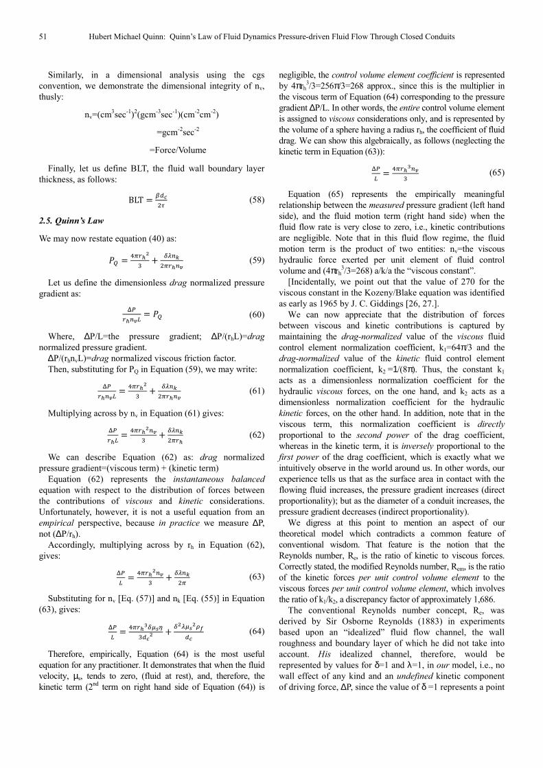
We hereby designate Equation (68) as Quinn’s Law of
Fluid Dynamics. It states that all pressure-driven flow in
closed conduits can be represented by a linear dimensionless
relationship, having a constant slope of 1/(8π) and an
intercept of 64π/3. This relationship is shown in Figure 12.
Figure 12. Quinn’s Law of Fluid Dynamics.
If we replace the velocity term in Equation (64) by a flow
rate term and substitute rh=4, we get:
∆U
= .'j|
+
hj\yz
(69)
In the special case of an empty conduit, where δ=1/8,
dc=D and π=22/7, it follows that we may write:
∆U
= .h|
+\yzh
(70)
Accordingly, we can conclude that in the case of an empty
conduit, the pressure gradient is:
a. inversely proportional to the fourth power of the
conduit diameter in the viscous term, and
b. inversely proportional to the fifth power of the conduit
diameter in the kinetic term.
Hence the empirical importance of measuring accurately
the conduit diameter in experiments related to conduit
permeability.
Finally, we point out that the viscous term in Equation (70)
corresponds to Poiseuille’s equation for laminar flow. Note,
however, that by comparison, Poiseuille’s equation has the
coefficient of π in the denominator, rather than the coefficient
of 3 in Equation (70). Therefore, Poiseuille’s equation
understates the pressure gradient by 1 part in 22, a
discrepancy of 4.55%, which falls within the measurement
error of many typical engineering applications.
Let us now consider a quadratic relationship for the
volumetric fluid flow, q, by expressing Equation (69) above,
as follows:
aq2+bq+c=0 (71)
Where, b=a variable coefficient of q; a=a variable
coefficient of q2; and c=a constant.
Rearranging Equation (71) gives:
aq2+bq=- c (72)
Substituting ∆P for –c in Equation (72) and rearranging
gives:
∆P=aq2+bq (73)
Solving Equation (73) for q gives:
53 Hubert Michael Quinn: Quinn’s Law of Fluid Dynamics Pressure-driven Fluid Flow Through Closed Conduits
q = /E±E[>∆U
> (74)
Let us define the coefficients a and b as follows:
a =hj\yz
(75)
b =.'j|
(76)
Substituting for a and b in Equation (73), we get Eq. (69):
∆U
=
.'j|
+
hj\yz
In order to cross-reference with the conventional literature
for packed conduits, we may now substitute for HQC
variables as follows:
Substituting for dc [Eq. (24)] and δ [Eq.(41)] in Equation
(69), and rearranging gives:
∆U
=
.'(./0@(|
+
h(./0@(\yz
0@ (77)
Switching the fluid flow parameter from volumetric flow
rate to superficial velocity, we may now write:
∆U
=
(./0@(x1|
0@ +
(./0@(\yzx1
0@ (78)
Substituting for 256π/3=A, on the left hand side of
Equation (78), and λ/(2πε03)=B, on the right hand side of
Equation (78), gives:
∆U
=
e(./0@(x1|
0@ +
(./0@(yzx1
0@ (79)
We point out that Equation (79) corresponds to the general
format of the Ergun equation. However, we call it the Q-
modified Ergun equation because the “constants” of A=268
(approx.) and B= λ/(2πε03), have been modified from Ergun’s
original constant values of 150 and 1.75 for A and B,
respectively, and most importantly, B is not a constant, but
rather is a function of both λ and ε0.
3. Results-Modeling the HQC as a
Harmonic Oscillator
3.1. The Spatial Coordinates
We shall now return to the motion of the fluid within the
HQC and describe it in terms of its instantaneous velocity
coordinates in three dimensions, i.e., x, y, z.
Thus, we may write:
v=vx + vy + vz (80)
where, v=the total instantaneous velocity.
Let us define the conduit frictional time interval as
follows:
' =0+
(81)
Where, t0=time to displace one conduit volume of fluid.
Let us define the wall shear stress as follows:
=∆U
(82)
Where, τw=the wall shear stress.
Let us define the frictional fluid velocity as follows:
µf=√(τw/ρf) (83)
Where, µf=the frictional fluid velocity.
Let us define the period of the fluid motion as follows:
T =q
(84)
Where, Τ=the period of the fluid motion.
Let us define the frequency of the fluid motion as follows:
φ = . (85)
Where, φ=the frequency of the fluid motion.
Let us define the maximum displacement amplitude of the
fluid motion as follows:
M' =
(86)
Where, M0=the maximum displacement amplitude of the
fluid motion (scale factor).
Let us define the instantaneous displacement amplitude as
follows:
M = M0exp(-ωt0)
(87)
Where, Μ=the instantaneous displacement amplitude of
the fluid motion.
Note that the negative sign in the exponent in equation
(87) represents the fact that the conduit wall frictional force
acts in the opposite direction to the fluid motion and, hence,
the motion is “damped” by wall friction.
Let us define the instantaneous displacement amplitude in
the x-axis plane as follows:
x = McosPQ (88)
Where, x=the instantaneous fluid displacement amplitude
in the x-axis plane.
Let us define the instantaneous fluid velocity in the x-axis
plane as follows:
v=/
∅ (89)
Where, vx=the instantaneous fluid velocity in the x-axis
plane.
Let us define the instantaneous fluid acceleration in the x-
axis plane as follows:
f=/(
∅ (90)
Where, fx=the instantaneous fluid acceleration in the x-axis
plane.
Fluid Mechanics 2019; 5(2): 39-71 54
Let us define the instantaneous motion displacement in the
y-axis plane as follows:
y = MsinPQ (91)
Where, y=the instantaneous fluid displacement in the y-
axis plane.
Let us define the instantaneous fluid velocity in the y-axis
plane as follows:
v¡=
∅ (92)
Where, vy=the instantaneous fluid velocity in the y-axis
plane.
Let us define the instantaneous fluid acceleration in the y-
axis plane as follows:
f¡=/
∅ (93)
Where, fy=the instantaneous fluid acceleration in the y-axis
plane.
Let us define the instantaneous motion displacement in the
z-axis plane as follows:
z = Mcos(π/4-PQ) (94)
Where, z=the instantaneous fluid displacement in the z-
axis plane.
Let us define the instantaneous fluid velocity in the z-axis
plane as follows:
vz=
/#//(
∅ (95)
Where, vz=the instantaneous fluid velocity in the z-axis
plane.
Let us define the instantaneous fluid acceleration in the z-
axis plane as follows:
F¤=/(//(
∅ (96)
Where, fz=the instantaneous fluid acceleration in the z-axis
plane.
3. 2. The Hypothetical Q Unit Cell
We shall now describe the dimensionless manifestation of
the fluid motion in the HQC which we term the
“Hypothetical Q Unit Cell” (HQUC).
Let us define the dimensionless instantaneous motion
displacement in the x-axis plane as follows:
x*=
@ (97)
Where, x*=the dimensionless instantaneous fluid
displacement in the x-axis plane.
Let us define the dimensionless instantaneous fluid
velocity in the x-axis plane as follows:
vz* =¥¦x§
(98)
Where, vx*=the dimensionless instantaneous fluid velocity
in the x-axis plane.
Let us define the dimensionless instantaneous motion
displacement in the y-axis plane as follows:
y* = ¡
@ (99)
Where, y*=the dimensionless instantaneous fluid
displacement in the y-axis plane.
Let us define the dimensionless instantaneous fluid
velocity in the y-axis plane as follows:
vy* =¥¨x§
(100)
Where, vy*=the dimensionless instantaneous fluid velocity
in the y-axis plane.
Let us define the dimensionless instantaneous motion
displacement in the z-axis plane as follows:
z* = ¤
@ (101)
Where, z*=the dimensionless instantaneous fluid
displacement in the x-axis plane.
Let us define the dimensionless instantaneous fluid
velocity in the z-axis plane as follows:
vz* =¥©x§
(102)
Where, vz*=the dimensionless instantaneous fluid velocity
in the z-axis plane.
4. Discussion-Exploring the QFFM
In order to further explore the implications of the HQC, we
propose a series of worked examples which will articulate the
role of the various parameters embodied in the QFFM. Our
worked examples have the following common independent
working variables: D=0.46 cm; L=10 cm; Ωp=1.0; dp=0.001
cm; η =0.01 poise; and ρf=1.0 g/mL.
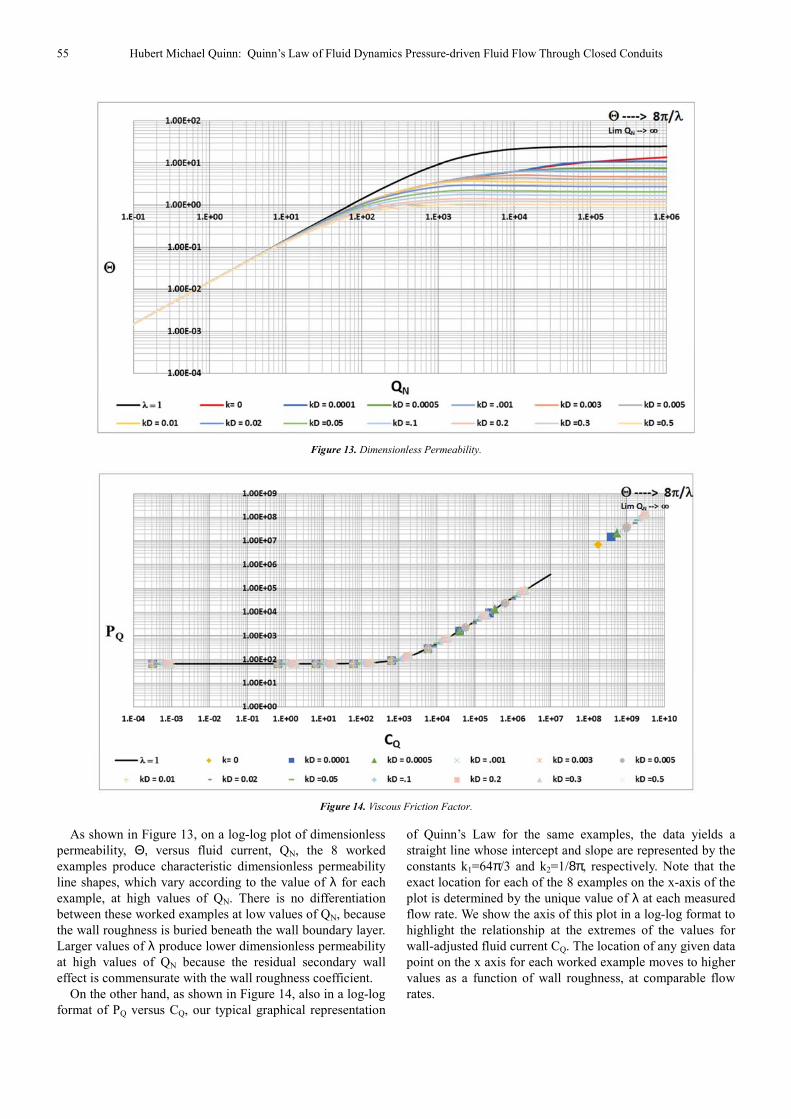
4.1. The HQC Fluid Current Normalization Coefficient λ
We begin with 8 worked examples involving an empty
conduit having variable relative wall roughness (kdc) values,
as shown in Figures 13 and 14. They are as follows:
1. Empty conduit-smooth wall (kdc=0)
2. Empty conduit-roughened wall (kdc=0.0001)
3. Empty conduit-roughened wall (kdc=0.001)
4. Empty conduit-roughened wall (kdc=0.01)
5. Empty conduit-roughened wall (kdc=0.03)
6. Empty conduit-roughened wall (kdc=0.05)
7. Empty conduit-roughened wall (kdc=0.1)
8. Empty conduit-roughened wall (kdc=0.5)
55 Hubert Michael Quinn: Quinn’s Law of Fluid Dynamics Pressure-driven Fluid Flow Through Closed Conduits
Figure 13. Dimensionless Permeability.
Figure 14. Viscous Friction Factor.
As shown in Figure 13, on a log-log plot of dimensionless
permeability, Θ, versus fluid current, QN, the 8 worked
examples produce characteristic dimensionless permeability
line shapes, which vary according to the value of λ for each
example, at high values of QN. There is no differentiation
between these worked examples at low values of QN, because
the wall roughness is buried beneath the wall boundary layer.
Larger values of λ produce lower dimensionless permeability
at high values of QN because the residual secondary wall
effect is commensurate with the wall roughness coefficient.
On the other hand, as shown in Figure 14, also in a log-log
format of PQ versus CQ, our typical graphical representation
of Quinn’s Law for the same examples, the data yields a
straight line whose intercept and slope are represented by the
constants k1=64π/3 and k2=1/8π, respectively. Note that the
exact location for each of the 8 examples on the x-axis of the
plot is determined by the unique value of λ at each measured
flow rate. We show the axis of this plot in a log-log format to
highlight the relationship at the extremes of the values for
wall-adjusted fluid current CQ. The location of any given data
point on the x axis for each worked example moves to higher
values as a function of wall roughness, at comparable flow
rates.
Fluid Mechanics 2019; 5(2): 39-71 56
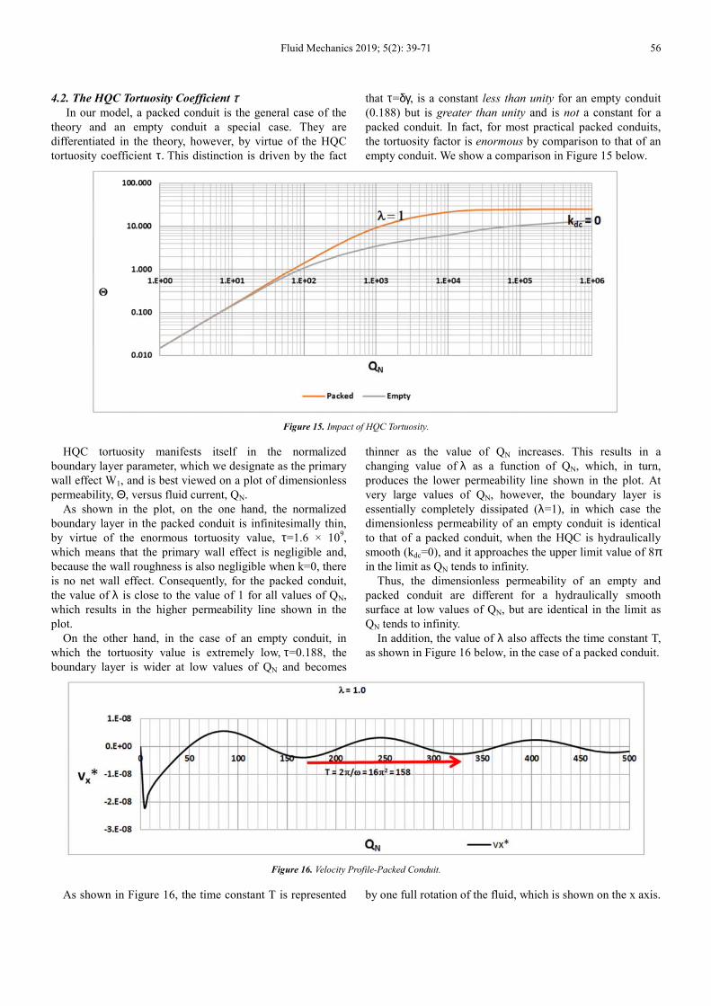
4.2. The HQC Tortuosity Coefficient τ
In our model, a packed conduit is the general case of the
theory and an empty conduit a special case. They are
differentiated in the theory, however, by virtue of the HQC
tortuosity coefficient τ. This distinction is driven by the fact
that τ=δγ, is a constant less than unity for an empty conduit
(0.188) but is greater than unity and is not a constant for a
packed conduit. In fact, for most practical packed conduits,
the tortuosity factor is enormous by comparison to that of an
empty conduit. We show a comparison in Figure 15 below.
Figure 15. Impact of HQC Tortuosity.
HQC tortuosity manifests itself in the normalized
boundary layer parameter, which we designate as the primary
wall effect W1, and is best viewed on a plot of dimensionless
permeability, Θ, versus fluid current, QN.
As shown in the plot, on the one hand, the normalized
boundary layer in the packed conduit is infinitesimally thin,
by virtue of the enormous tortuosity value, τ=1.6 × 10⁹,
which means that the primary wall effect is negligible and,
because the wall roughness is also negligible when k=0, there
is no net wall effect. Consequently, for the packed conduit,
the value of λ is close to the value of 1 for all values of QN,
which results in the higher permeability line shown in the
plot.
On the other hand, in the case of an empty conduit, in
which the tortuosity value is extremely low, τ=0.188, the
boundary layer is wider at low values of QN and becomes
thinner as the value of QN increases. This results in a
changing value of λ as a function of QN, which, in turn,
produces the lower permeability line shown in the plot. At
very large values of QN, however, the boundary layer is
essentially completely dissipated (λ=1), in which case the
dimensionless permeability of an empty conduit is identical
to that of a packed conduit, when the HQC is hydraulically
smooth (kdc=0), and it approaches the upper limit value of 8π
in the limit as QN tends to infinity.
Thus, the dimensionless permeability of an empty and
packed conduit are different for a hydraulically smooth
surface at low values of QN, but are identical in the limit as
QN tends to infinity.
In addition, the value of λ also affects the time constant T,
as shown in Figure 16 below, in the case of a packed conduit.
Figure 16. Velocity Profile-Packed Conduit.
As shown in Figure 16, the time constant T is represented by one full rotation of the fluid, which is shown on the x axis.
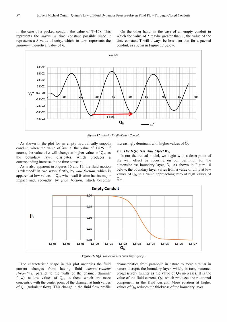
57 Hubert Michael Quinn: Quinn’s Law of Fluid Dynamics Pressure-driven Fluid Flow Through Closed Conduits
In the case of a packed conduit, the value of T=158. This
represents the maximum time constant possible since it
represents a λ value of unity, which, in turn, represents the
minimum theoretical value of λ.
On the other hand, in the case of an empty conduit in
which the value of λ maybe greater than 1, the value of the
time constant T will always be less than that for a packed
conduit, as shown in Figure 17 below.
Figure 17. Velocity Profile-Empty Conduit.
As shown in the plot for an empty hydraulically smooth
conduit, when the value of λ=6.3, the value of T=25. Of
course, the value of λ will change at higher values of QN, as
the boundary layer dissipates, which produces a
corresponding increase in the time constant.
As is also apparent in Figures 16 and 17, the fluid motion
is “damped” in two ways; firstly, by wall friction, which is
apparent at low values of QN, when wall friction has its major
impact and, secondly, by fluid friction, which becomes
increasingly dominant with higher values of QN.
4.3. The HQC Net Wall Effect WN
In our theoretical model, we begin with a description of
the wall effect by focusing on our definition for the
dimensionless boundary layer, β0. As shown in Figure 18
below, the boundary layer varies from a value of unity at low
values of QN to a value approaching zero at high values of
QN.
Figure 18. HQC Dimensionless Boundary Layer β0.
The characteristic shape in this plot underlies the fluid
current changes from having fluid current-velocity
streamlines parallel to the walls of the channel (laminar
flow), at low values of QN, to those which are more
concentric with the center point of the channel, at high values
of QN (turbulent flow). This change in the fluid flow profile
characteristics from parabolic in nature to more circular in
nature disrupts the boundary layer, which, in turn, becomes
progressively thinner as the value of QN increases. It is the
value of the fluid current, QN, which produces the rotational
component in the fluid current. More rotation at higher
values of QN reduces the thickness of the boundary layer.
Fluid Mechanics 2019; 5(2): 39-71 58
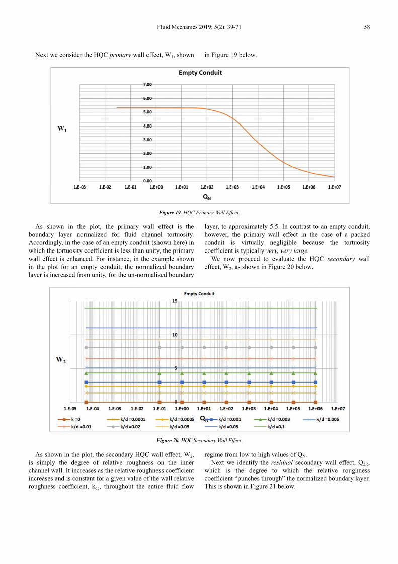
Next we consider the HQC primary wall effect, W1, shown in Figure 19 below.
Figure 19. HQC Primary Wall Effect.
As shown in the plot, the primary wall effect is the
boundary layer normalized for fluid channel tortuosity.
Accordingly, in the case of an empty conduit (shown here) in
which the tortuosity coefficient is less than unity, the primary
wall effect is enhanced. For instance, in the example shown
in the plot for an empty conduit, the normalized boundary
layer is increased from unity, for the un-normalized boundary
layer, to approximately 5.5. In contrast to an empty conduit,
however, the primary wall effect in the case of a packed
conduit is virtually negligible because the tortuosity
coefficient is typically very, very large.
We now proceed to evaluate the HQC secondary wall
effect, W2, as shown in Figure 20 below.
Figure 20. HQC Secondary Wall Effect.
As shown in the plot, the secondary HQC wall effect, W2,
is simply the degree of relative roughness on the inner
channel wall. It increases as the relative roughness coefficient
increases and is constant for a given value of the wall relative
roughness coefficient, kdc, throughout the entire fluid flow
regime from low to high values of QN.
Next we identify the residual secondary wall effect, Q2R,
which is the degree to which the relative roughness
coefficient “punches through” the normalized boundary layer.
This is shown in Figure 21 below.
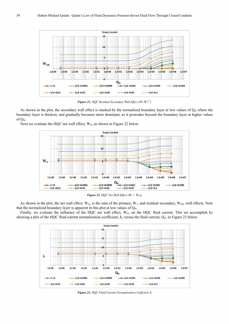
59 Hubert Michael Quinn: Quinn’s Law of Fluid Dynamics Pressure-driven Fluid Flow Through Closed Conduits
Figure 21. HQC Residual Secondary Wall Effect (W2-W11.2).
As shown in the plot, the secondary wall effect is masked by the normalized boundary layer at low values of QN where the
boundary layer is thickest, and gradually becomes more dominant, as it protrudes beyond the boundary layer at higher values
of QN.
Next we evaluate the HQC net wall effect, WN, as shown in Figure 22 below.
Figure 22. HQC Net Wall Effect (W1 + W2R).
As shown in the plot, the net wall effect, WN, is the sum of the primary, W1, and residual secondary, W2R, wall effects. Note
that the normalized boundary layer is apparent in this plot at low values of QN.
Finally, we evaluate the influence of the HQC net wall effect, WN, on the HQC fluid current. This we accomplish by
showing a plot of the HQC fluid current normalization coefficient, λ, versus the fluid current, QN, in Figure 23 below.
Figure 23. HQC Fluid Current Normalization Coefficient λ.
Fluid Mechanics 2019; 5(2): 39-71 60
As shown in the plot, the normalized fluid current is
relatively constant at low values of QN and reaches a plateau
which may be greater or less than the primary wall effect,
commensurate with relative wall roughness.
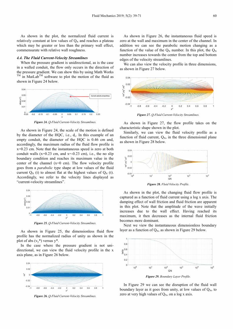
4.4. The Fluid Current-Velocity Streamlines
When the pressure gradient is unidirectional, as is the case
in a walled conduit, the flow only occurs in the direction of
the pressure gradient. We can show this by using Math Works TM
in MatLabTM
software to plot the motion of the fluid as
shown in Figure 24 below.
Figure 24. Q-Fluid Current-Velocity Streamlines.
As shown in Figure 24, the scale of the motion is defined
by the diameter of the HQC, i.e., dc. In this example of an
empty conduit, the diameter of the HQC is 0.46 cm and,
accordingly, the maximum radius of the fluid flow profile is
x=0.23 cm. Note that the instantaneous speed is zero at both
conduit walls (x=0.23 cm, and x=-0.23 cm), i.e., the no slip
boundary condition and reaches its maximum value in the
center of the channel (x=0 cm). The flow velocity profile
goes from a parabolic type shape at low values of the fluid
current QN (t) to almost flat at the highest values of QN (t).
Accordingly, we refer to the velocity lines displayed as
“current-velocity streamlines”.
Figure 25. Q-Fluid Current-Velocity Streamlines.
As shown in Figure 25, the dimensionless fluid flow
profile has the normalized radius of unity as shown in the
plot of abs (vy*) versus y*.
In the case where the pressure gradient is not uni-
directional, we can view the fluid velocity profile in the x
axis plane, as in Figure 26 below.
Figure 26. Q-Fluid Current-Velocity Streamlines.
As shown in Figure 26, the instantaneous fluid speed is
zero at the wall and maximum in the center of the channel. In
addition we can see the parabolic motion changing as a
function of the value of the QN number. In this plot, the QN
number increases towards the center from the top and bottom
edges of the velocity streamlines.
We can also view the velocity profile in three dimensions,
as shown in Figure 27 below.
Figure 27. Q-Fluid Current-Velocity Streamlines.
As shown in Figure 27, the flow profile takes on the
characteristic shape shown in the plot.
Similarly, we can view the fluid velocity profile as a
function of fluid current, QN, in the three dimensional plane
as shown in Figure 28 below.
Figure 28. Fluid Velocity Profile.
As shown in the plot, the changing fluid flow profile is
captured as a function of fluid current using a log x axis. The
damping effect of wall friction and fluid friction are apparent
in this plot. Note that the amplitude of the wave initially
increases due to the wall effect. Having reached its
maximum, it then decreases as the internal fluid friction
becomes more dominant.
Next we view the instantaneous dimensionless boundary
layer as a function of QN, as shown in Figure 29 below.
Figure 29. Boundary Layer Profile.
In Figure 29 we can see the disruption of the fluid wall
boundary layer as it goes from unity, at low values of QN, to
zero at very high values of QN, on a log x axis.
61 Hubert Michael Quinn: Quinn’s Law of Fluid Dynamics Pressure-driven Fluid Flow Through Closed Conduits
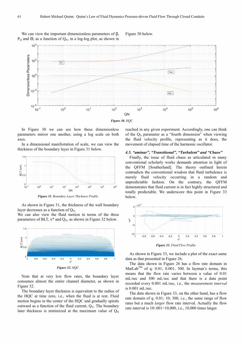
We can view the important dimensionless parameters of β,
PQ and Θ, as a function of QN, in a log-log plot, as shown in
Figure 30 below.
Figure 30. HQC.
In Figure 30 we can see how these dimensionless
parameters mirror one another, using a log scale on both
axes.
In a dimensional manifestation of scale, we can view the
thickness of the boundary layer in Figure 31 below.
Figure 31. Boundary Layer Thickness Profile.
As shown in Figure 31, the thickness of the wall boundary
layer decreases as a function of QN.
We can also view the fluid motion in terms of the three
parameters of BLT, x* and QN, as shown in Figure 32 below.
Figure 32. HQC.
Note that at very low flow rates, the boundary layer
consumes almost the entire channel diameter, as shown in
Figure 32.
The boundary layer thickness is equivalent to the radius of
the HQC at time zero, i.e., when the fluid is at rest. Fluid
motion begins in the center of the HQC and gradually spirals
outward as a function of the fluid current, QN. The boundary
later thickness is minimized at the maximum value of QN
reached in any given experiment. Accordingly, one can think
of the QN parameter as a “fourth dimension” when viewing
the fluid velocity profile, representing as it does, the
movement of elapsed time of the harmonic oscillator.
4.5. “aminar”, “Transitional”, “Turbulent” and “Chaos”
Finally, the issue of fluid chaos as articulated in many
conventional scholarly works demands attention in light of
the QFFM [Southerland]. The theory outlined herein
contradicts the conventional wisdom that fluid turbulence is
merely fluid velocity occurring in a random and
unpredictable fashion. On the contrary, the QFFM
demonstrates that fluid current is in fact highly structured and
totally predictable. We underscore this point in Figure 33
below.
Figure 33. Fluid Flow Profile.
As shown in Figure 33, we include a plot of the exact same
data as that presented in Figure 26.
The data shown in Figure 26 has a flow rate domain in
MatLabTM
of q: 0.01; 0.001; 300. In layman’s terms, this
means that the flow rate varies between a value of 0.01
mL/sec and 300 mL/sec and that there is a data point
recorded every 0.001 mL/sec, i.e., the measurement interval
is 0.001 mL/sec.
The data shown in Figure 33, on the other hand, has a flow
rate domain of q: 0.01; 10; 300, i.e., the same range of flow
rates but a much larger flow rate interval. Actually the flow
rate interval is 10/.001=10,000, i.e., 10,000 times larger.
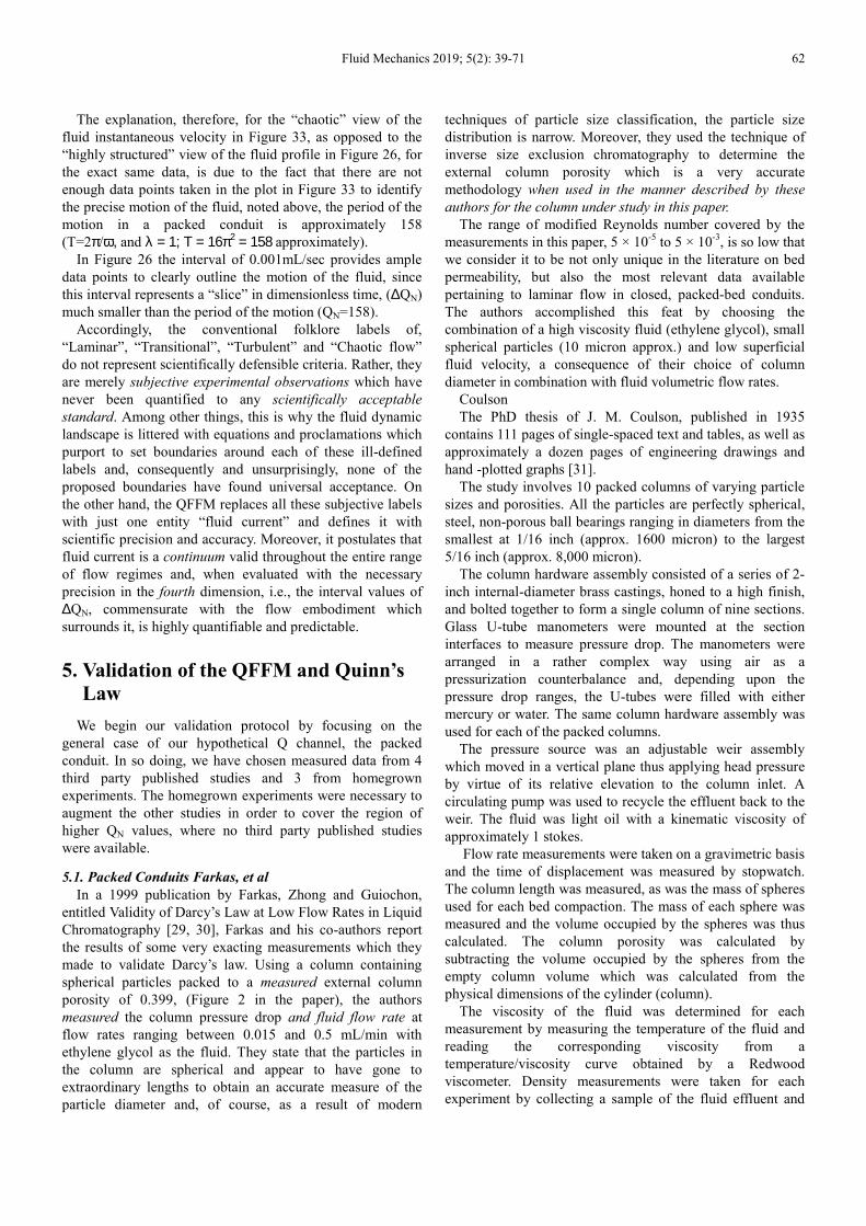
Fluid Mechanics 2019; 5(2): 39-71 62
The explanation, therefore, for the “chaotic” view of the
fluid instantaneous velocity in Figure 33, as opposed to the
“highly structured” view of the fluid profile in Figure 26, for
the exact same data, is due to the fact that there are not
enough data points taken in the plot in Figure 33 to identify
the precise motion of the fluid, noted above, the period of the
motion in a packed conduit is approximately 158
(T=2π/ω, and λ = 1; Τ = 16π2 = 158 approximately).
In Figure 26 the interval of 0.001mL/sec provides ample
data points to clearly outline the motion of the fluid, since
this interval represents a “slice” in dimensionless time, (∆QN)
much smaller than the period of the motion (QN=158).
Accordingly, the conventional folklore labels of,
“Laminar”, “Transitional”, “Turbulent” and “Chaotic flow”
do not represent scientifically defensible criteria. Rather, they
are merely subjective experimental observations which have
never been quantified to any scientifically acceptable
standard. Among other things, this is why the fluid dynamic
landscape is littered with equations and proclamations which
purport to set boundaries around each of these ill-defined
labels and, consequently and unsurprisingly, none of the
proposed boundaries have found universal acceptance. On
the other hand, the QFFM replaces all these subjective labels
with just one entity “fluid current” and defines it with
scientific precision and accuracy. Moreover, it postulates that
fluid current is a continuum valid throughout the entire range
of flow regimes and, when evaluated with the necessary
precision in the fourth dimension, i.e., the interval values of
∆QN, commensurate with the flow embodiment which
surrounds it, is highly quantifiable and predictable.
5. Validation of the QFFM and Quinn’s
Law
We begin our validation protocol by focusing on the
general case of our hypothetical Q channel, the packed
conduit. In so doing, we have chosen measured data from 4
third party published studies and 3 from homegrown
experiments. The homegrown experiments were necessary to
augment the other studies in order to cover the region of
higher QN values, where no third party published studies
were available.
5.1. Packed Conduits Farkas, et al
In a 1999 publication by Farkas, Zhong and Guiochon,
entitled Validity of Darcy’s Law at Low Flow Rates in Liquid
Chromatography [29, 30], Farkas and his co-authors report
the results of some very exacting measurements which they
made to validate Darcy’s law. Using a column containing
spherical particles packed to a measured external column
porosity of 0.399, (Figure 2 in the paper), the authors
measured the column pressure drop and fluid flow rate at
flow rates ranging between 0.015 and 0.5 mL/min with
ethylene glycol as the fluid. They state that the particles in
the column are spherical and appear to have gone to
extraordinary lengths to obtain an accurate measure of the
particle diameter and, of course, as a result of modern
techniques of particle size classification, the particle size
distribution is narrow. Moreover, they used the technique of
inverse size exclusion chromatography to determine the
external column porosity which is a very accurate
methodology when used in the manner described by these
authors for the column under study in this paper.
The range of modified Reynolds number covered by the
measurements in this paper, 5 × 10⁻⁵
to 5 × 10⁻³
, is so low that
we consider it to be not only unique in the literature on bed
permeability, but also the most relevant data available
pertaining to laminar flow in closed, packed-bed conduits.
The authors accomplished this feat by choosing the
combination of a high viscosity fluid (ethylene glycol), small
spherical particles (10 micron approx.) and low superficial
fluid velocity, a consequence of their choice of column
diameter in combination with fluid volumetric flow rates.
Coulson
The PhD thesis of J. M. Coulson, published in 1935
contains 111 pages of single-spaced text and tables, as well as
approximately a dozen pages of engineering drawings and
hand -plotted graphs [31].
The study involves 10 packed columns of varying particle
sizes and porosities. All the particles are perfectly spherical,
steel, non-porous ball bearings ranging in diameters from the
smallest at 1/16 inch (approx. 1600 micron) to the largest
5/16 inch (approx. 8,000 micron).
The column hardware assembly consisted of a series of 2-
inch internal-diameter brass castings, honed to a high finish,
and bolted together to form a single column of nine sections.
Glass U-tube manometers were mounted at the section
interfaces to measure pressure drop. The manometers were
arranged in a rather complex way using air as a
pressurization counterbalance and, depending upon the
pressure drop ranges, the U-tubes were filled with either
mercury or water. The same column hardware assembly was
used for each of the packed columns.
The pressure source was an adjustable weir assembly
which moved in a vertical plane thus applying head pressure
by virtue of its relative elevation to the column inlet. A
circulating pump was used to recycle the effluent back to the
weir. The fluid was light oil with a kinematic viscosity of
approximately 1 stokes.
Flow rate measurements were taken on a gravimetric basis
and the time of displacement was measured by stopwatch.
The column length was measured, as was the mass of spheres
used for each bed compaction. The mass of each sphere was
measured and the volume occupied by the spheres was thus
calculated. The column porosity was calculated by
subtracting the volume occupied by the spheres from the
empty column volume which was calculated from the
physical dimensions of the cylinder (column).
The viscosity of the fluid was determined for each
measurement by measuring the temperature of the fluid and
reading the corresponding viscosity from a
temperature/viscosity curve obtained by a Redwood
viscometer. Density measurements were taken for each
experiment by collecting a sample of the fluid effluent and
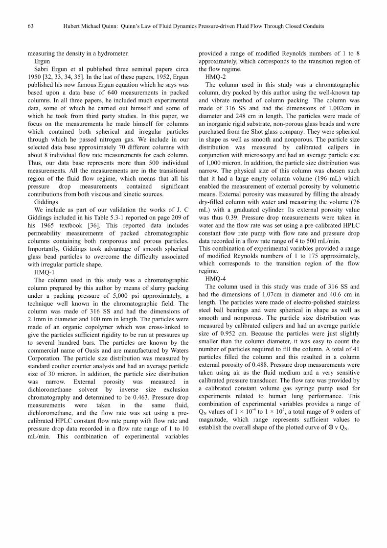
63 Hubert Michael Quinn: Quinn’s Law of Fluid Dynamics Pressure-driven Fluid Flow Through Closed Conduits
measuring the density in a hydrometer.
Ergun
Sabri Ergun et al published three seminal papers circa
1950 [32, 33, 34, 35]. In the last of these papers, 1952, Ergun
published his now famous Ergun equation which he says was
based upon a data base of 640 measurements in packed
columns. In all three papers, he included much experimental
data, some of which he carried out himself and some of
which he took from third party studies. In this paper, we
focus on the measurements he made himself for columns
which contained both spherical and irregular particles
through which he passed nitrogen gas. We include in our
selected data base approximately 70 different columns with
about 8 individual flow rate measurements for each column.
Thus, our data base represents more than 500 individual
measurements. All the measurements are in the transitional
region of the fluid flow regime, which means that all his
pressure drop measurements contained significant
contributions from both viscous and kinetic sources.
Giddings
We include as part of our validation the works of J. C
Giddings included in his Table 5.3-1 reported on page 209 of
his 1965 textbook [36]. This reported data includes
permeability measurements of packed chromatographic
columns containing both nonporous and porous particles.
Importantly, Giddings took advantage of smooth spherical
glass bead particles to overcome the difficulty associated
with irregular particle shape.
HMQ-1
The column used in this study was a chromatographic
column prepared by this author by means of slurry packing
under a packing pressure of 5,000 psi approximately, a
technique well known in the chromatographic field. The
column was made of 316 SS and had the dimensions of
2.1mm in diameter and 100 mm in length. The particles were
made of an organic copolymer which was cross-linked to
give the particles sufficient rigidity to be run at pressures up
to several hundred bars. The particles are known by the
commercial name of Oasis and are manufactured by Waters
Corporation. The particle size distribution was measured by
standard coulter counter analysis and had an average particle
size of 30 micron. In addition, the particle size distribution
was narrow. External porosity was measured in
dichloromethane solvent by inverse size exclusion
chromatography and determined to be 0.463. Pressure drop
measurements were taken in the same fluid,
dichloromethane, and the flow rate was set using a pre-
calibrated HPLC constant flow rate pump with flow rate and
pressure drop data recorded in a flow rate range of 1 to 10
mL/min. This combination of experimental variables
provided a range of modified Reynolds numbers of 1 to 8
approximately, which corresponds to the transition region of
the flow regime.
HMQ-2
The column used in this study was a chromatographic
column, dry packed by this author using the well-known tap
and vibrate method of column packing. The column was
made of 316 SS and had the dimensions of 1.002cm in
diameter and 248 cm in length. The particles were made of
an inorganic rigid substrate, non-porous glass beads and were
purchased from the Shot glass company. They were spherical
in shape as well as smooth and nonporous. The particle size
distribution was measured by calibrated calipers in
conjunction with microscopy and had an average particle size
of 1,000 micron. In addition, the particle size distribution was
narrow. The physical size of this column was chosen such
that it had a large empty column volume (196 mL) which
enabled the measurement of external porosity by volumetric
means. External porosity was measured by filling the already
dry-filled column with water and measuring the volume (76
mL) with a graduated cylinder. Its external porosity value
was thus 0.39. Pressure drop measurements were taken in
water and the flow rate was set using a pre-calibrated HPLC
constant flow rate pump with flow rate and pressure drop
data recorded in a flow rate range of 4 to 500 mL/min.
This combination of experimental variables provided a range
of modified Reynolds numbers of 1 to 175 approximately,
which corresponds to the transition region of the flow
regime.
HMQ-4
The column used in this study was made of 316 SS and
had the dimensions of 1.07cm in diameter and 40.6 cm in
length. The particles were made of electro-polished stainless
steel ball bearings and were spherical in shape as well as
smooth and nonporous. The particle size distribution was
measured by calibrated calipers and had an average particle
size of 0.952 cm. Because the particles were just slightly
smaller than the column diameter, it was easy to count the
number of particles required to fill the column. A total of 41
particles filled the column and this resulted in a column
external porosity of 0.488. Pressure drop measurements were
taken using air as the fluid medium and a very sensitive
calibrated pressure transducer. The flow rate was provided by
a calibrated constant volume gas syringe pump used for
experiments related to human lung performance. This
combination of experimental variables provides a range of
QN values of 1 × 10⁻⁴
to 1 × 10⁵, a total range of 9 orders of
magnitude, which range represents sufficient values to
establish the overall shape of the plotted curve of Θ v QN.
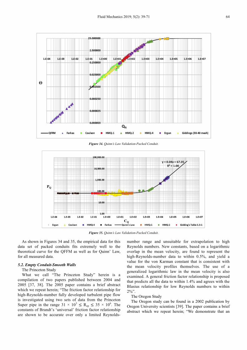
Fluid Mechanics 2019; 5(2): 39-71 64
Figure 34. Quinn’s Law Validation-Packed Conduit.
Figure 35. Quinn’s Law Validation-Packed Conduit.
As shown in Figures 34 and 35, the empirical data for this
data set of packed conduits fits extremely well to the
theoretical curve for the QFFM as well as for Quinn’ Law,
for all measured data.
5.2. Empty Conduit-Smooth Walls
The Princeton Study
What we call “The Princeton Study” herein is a
compilation of two papers published between 2004 and
2005 [37, 38]. The 2005 paper contains a brief abstract
which we repeat herein; “The friction factor relationship for
high-Reynolds-number fully developed turbulent pipe flow
is investigated using two sets of data from the Princeton
Super pipe in the range 31 × 103 ≤ Rep ≤ 35 × 10
6. The
constants of Brandt’s ‘universal’ friction factor relationship
are shown to be accurate over only a limited Reynolds-
number range and unsuitable for extrapolation to high
Reynolds numbers. New constants, based on a logarithmic
overlap in the mean velocity, are found to represent the
high-Reynolds-number data to within 0.5%, and yield a
value for the von Karman constant that is consistent with
the mean velocity profiles themselves. The use of a
generalized logarithmic law in the mean velocity is also
examined. A general friction factor relationship is proposed
that predicts all the data to within 1.4% and agrees with the
Blasius relationship for low Reynolds numbers to within
2%”.
The Oregon Study
The Oregon study can be found in a 2002 publication by
Oregon University scientists [39]. The paper contains a brief
abstract which we repeat herein; “We demonstrate that an
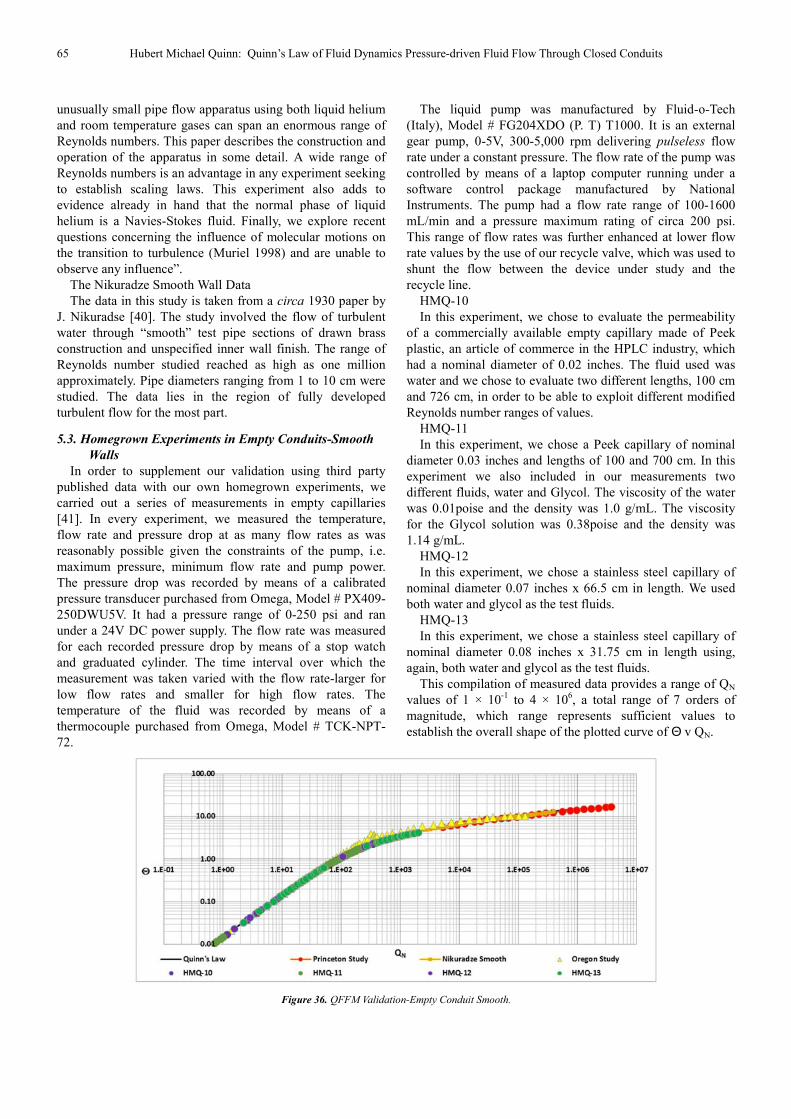
65 Hubert Michael Quinn: Quinn’s Law of Fluid Dynamics Pressure-driven Fluid Flow Through Closed Conduits
unusually small pipe flow apparatus using both liquid helium
and room temperature gases can span an enormous range of
Reynolds numbers. This paper describes the construction and
operation of the apparatus in some detail. A wide range of
Reynolds numbers is an advantage in any experiment seeking
to establish scaling laws. This experiment also adds to
evidence already in hand that the normal phase of liquid
helium is a Navies-Stokes fluid. Finally, we explore recent
questions concerning the influence of molecular motions on
the transition to turbulence (Muriel 1998) and are unable to
observe any influence”.
The Nikuradze Smooth Wall Data
The data in this study is taken from a circa 1930 paper by
J. Nikuradse [40]. The study involved the flow of turbulent
water through “smooth” test pipe sections of drawn brass
construction and unspecified inner wall finish. The range of
Reynolds number studied reached as high as one million
approximately. Pipe diameters ranging from 1 to 10 cm were
studied. The data lies in the region of fully developed
turbulent flow for the most part.
5.3. Homegrown Experiments in Empty Conduits-Smooth
Walls
In order to supplement our validation using third party
published data with our own homegrown experiments, we
carried out a series of measurements in empty capillaries
[41]. In every experiment, we measured the temperature,
flow rate and pressure drop at as many flow rates as was
reasonably possible given the constraints of the pump, i.e.
maximum pressure, minimum flow rate and pump power.
The pressure drop was recorded by means of a calibrated
pressure transducer purchased from Omega, Model # PX409-
250DWU5V. It had a pressure range of 0-250 psi and ran
under a 24V DC power supply. The flow rate was measured
for each recorded pressure drop by means of a stop watch
and graduated cylinder. The time interval over which the
measurement was taken varied with the flow rate-larger for
low flow rates and smaller for high flow rates. The
temperature of the fluid was recorded by means of a
thermocouple purchased from Omega, Model # TCK-NPT-
72.
The liquid pump was manufactured by Fluid-o-Tech
(Italy), Model # FG204XDO (P. T) T1000. It is an external
gear pump, 0-5V, 300-5,000 rpm delivering pulseless flow
rate under a constant pressure. The flow rate of the pump was
controlled by means of a laptop computer running under a
software control package manufactured by National
Instruments. The pump had a flow rate range of 100-1600
mL/min and a pressure maximum rating of circa 200 psi.
This range of flow rates was further enhanced at lower flow
rate values by the use of our recycle valve, which was used to
shunt the flow between the device under study and the
recycle line.
HMQ-10
In this experiment, we chose to evaluate the permeability
of a commercially available empty capillary made of Peek
plastic, an article of commerce in the HPLC industry, which
had a nominal diameter of 0.02 inches. The fluid used was
water and we chose to evaluate two different lengths, 100 cm
and 726 cm, in order to be able to exploit different modified
Reynolds number ranges of values.
HMQ-11
In this experiment, we chose a Peek capillary of nominal
diameter 0.03 inches and lengths of 100 and 700 cm. In this
experiment we also included in our measurements two
different fluids, water and Glycol. The viscosity of the water
was 0.01poise and the density was 1.0 g/mL. The viscosity
for the Glycol solution was 0.38poise and the density was
1.14 g/mL.
HMQ-12
In this experiment, we chose a stainless steel capillary of
nominal diameter 0.07 inches x 66.5 cm in length. We used
both water and glycol as the test fluids.
HMQ-13
In this experiment, we chose a stainless steel capillary of
nominal diameter 0.08 inches x 31.75 cm in length using,
again, both water and glycol as the test fluids.
This compilation of measured data provides a range of QN
values of 1 × 10⁻¹
to 4 × 10⁶, a total range of 7 orders of
magnitude, which range represents sufficient values to
establish the overall shape of the plotted curve of Θ v QN.
Figure 36. QFFM Validation-Empty Conduit Smooth.
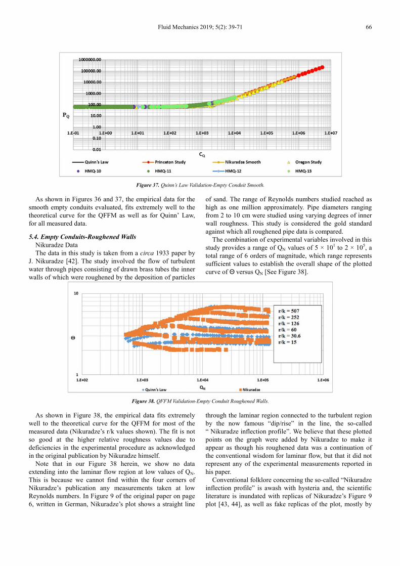
Fluid Mechanics 2019; 5(2): 39-71 66
Figure 37. Quinn’s Law Validation-Empty Conduit Smooth.
As shown in Figures 36 and 37, the empirical data for the
smooth empty conduits evaluated, fits extremely well to the
theoretical curve for the QFFM as well as for Quinn’ Law,
for all measured data.
5.4. Empty Conduits-Roughened Walls
Nikuradze Data
The data in this study is taken from a circa 1933 paper by
J. Nikuradze [42]. The study involved the flow of turbulent
water through pipes consisting of drawn brass tubes the inner
walls of which were roughened by the deposition of particles
of sand. The range of Reynolds numbers studied reached as
high as one million approximately. Pipe diameters ranging
from 2 to 10 cm were studied using varying degrees of inner
wall roughness. This study is considered the gold standard
against which all roughened pipe data is compared.
The combination of experimental variables involved in this
study provides a range of QN values of 5 × 101 to 2 × 10
5, a
total range of 6 orders of magnitude, which range represents
sufficient values to establish the overall shape of the plotted
curve of Θ versus QN [See Figure 38].
Figure 38. QFFM Validation-Empty Conduit Roughened Walls.
As shown in Figure 38, the empirical data fits extremely
well to the theoretical curve for the QFFM for most of the
measured data (Nikuradze’s r/k values shown). The fit is not
so good at the higher relative roughness values due to
deficiencies in the experimental procedure as acknowledged
in the original publication by Nikuradze himself.
Note that in our Figure 38 herein, we show no data
extending into the laminar flow region at low values of QN.
This is because we cannot find within the four corners of
Nikuradze’s publication any measurements taken at low
Reynolds numbers. In Figure 9 of the original paper on page
6, written in German, Nikuradze’s plot shows a straight line
through the laminar region connected to the turbulent region
by the now famous “dip/rise” in the line, the so-called
“ Nikuradze inflection profile”. We believe that these plotted
points on the graph were added by Nikuradze to make it
appear as though his roughened data was a continuation of
the conventional wisdom for laminar flow, but that it did not
represent any of the experimental measurements reported in
his paper.
Conventional folklore concerning the so-called “Nikuradze
inflection profile” is awash with hysteria and, the scientific
literature is inundated with replicas of Nikuradze’s Figure 9
plot [43, 44], as well as fake replicas of the plot, mostly by
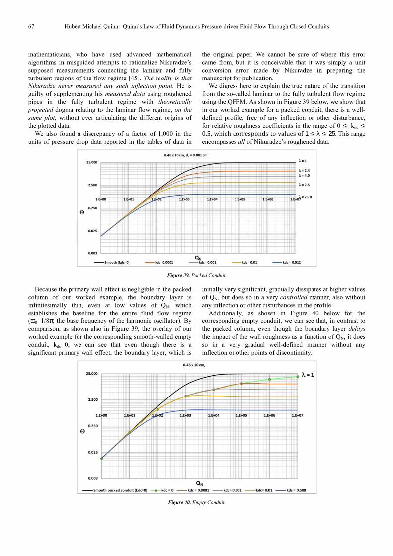
67 Hubert Michael Quinn: Quinn’s Law of Fluid Dynamics Pressure-driven Fluid Flow Through Closed Conduits
mathematicians, who have used advanced mathematical
algorithms in misguided attempts to rationalize Nikuradze’s
supposed measurements connecting the laminar and fully
turbulent regions of the flow regime [45]. The reality is that
Nikuradze never measured any such inflection point. He is
guilty of supplementing his measured data using roughened
pipes in the fully turbulent regime with theoretically
projected dogma relating to the laminar flow regime, on the
same plot, without ever articulating the different origins of
the plotted data.
We also found a discrepancy of a factor of 1,000 in the
units of pressure drop data reported in the tables of data in
the original paper. We cannot be sure of where this error
came from, but it is conceivable that it was simply a unit
conversion error made by Nikuradze in preparing the
manuscript for publication.
We digress here to explain the true nature of the transition
from the so-called laminar to the fully turbulent flow regime
using the QFFM. As shown in Figure 39 below, we show that
in our worked example for a packed conduit, there is a well-
defined profile, free of any inflection or other disturbance,
for relative roughness coefficients in the range of 0 ≤ kdc ≤0.5,whichcorrespondstovaluesof1 λ 25. This range
encompasses all of Nikuradze’s roughened data.
Figure 39. Packed Conduit.
Because the primary wall effect is negligible in the packed
column of our worked example, the boundary layer is
infinitesimally thin, even at low values of QN, which
establishes the baseline for the entire fluid flow regime
(ω0=1/8π, the base frequency of the harmonic oscillator). By
comparison, as shown also in Figure 39, the overlay of our
worked example for the corresponding smooth-walled empty
conduit, kdc=0, we can see that even though there is a
significant primary wall effect, the boundary layer, which is
initially very significant, gradually dissipates at higher values
of QN, but does so in a very controlled manner, also without
any inflection or other disturbances in the profile.
Additionally, as shown in Figure 40 below for the
corresponding empty conduit, we can see that, in contrast to
the packed column, even though the boundary layer delays
the impact of the wall roughness as a function of QN, it does
so in a very gradual well-defined manner without any
inflection or other points of discontinuity.
Figure 40. Empty Conduit.
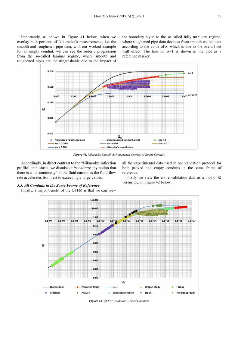
Fluid Mechanics 2019; 5(2): 39-71 68
Importantly, as shown in Figure 41 below, when we
overlay both portions of Nikuradze’s measurements, i.e. the
smooth and roughened pipe data, with our worked example
for an empty conduit, we can see the orderly progression
from the so-called laminar regime, where smooth and
roughened pipes are indistinguishable due to the impact of
the boundary layer, to the so-called fully turbulent regime,
where roughened pipe data deviates from smooth walled data
according to the value of λ, which is due to the overall net
wall effect. The line for λ=1 is shown in the plot as a
reference marker.
Figure 41. Nikuradze Smooth & Roughened Overlay of Empty Conduit.
Accordingly, in direct contrast to the “Nikuradze inflection
profile” enthusiasts, we dismiss in its entirety any notion that
there is a “discontinuity” in the fluid current as the fluid flow
rate accelerates from rest to exceedingly large values.
5.5. All Conduits in the Same Frame of Reference
Finally, a major benefit of the QFFM is that we can view
all the experimental data used in our validation protocol for
both packed and empty conduits in the same frame of
reference.
Firstly we view the entire validation data as a plot of Θ
versus QN, in Figure 42 below.
Figure 42. QFFM Validation-Closed Conduits.
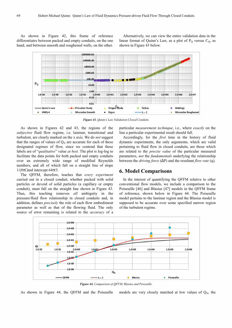
69 Hubert Michael Quinn: Quinn’s Law of Fluid Dynamics Pressure-driven Fluid Flow Through Closed Conduits
As shown in Figure 42, this frame of reference
differentiates between packed and empty conduits, on the one
hand, and between smooth and roughened walls, on the other.
Alternatively, we can view the entire validation data in the
linear format of Quinn’s Law, as a plot of PQ versus CQ, as
shown in Figure 43 below.
Figure 43. Quinn’s Law Validation-Closed Conduits.
As shown in Figures 42 and 43, the regions of the
subjective fluid flow regime, i.e. laminar, transitional and
turbulent, are clearly marked on the x axis. We do not suggest
that the ranges of values of QN are accurate for each of these
designated regimes of flow, since we contend that these
labels are of “qualitative” value at best. The plot is log-log to
facilitate the data points for both packed and empty conduits
over an extremely wide range of modified Reynolds
numbers, and all of which fall on a straight line of slope
1/(8π) and intercept 64π/3.
The QFFM, therefore, teaches that every experiment
carried out in a closed conduit, whether packed with solid
particles or devoid of solid particles (a capillary or empty
conduit), must fall on the straight line shown in Figure 43.
Thus, this teaching removes all ambiguity in the
pressure/fluid flow relationship in closed conduits and, in
addition, defines precisely the role of each flow embodiment
parameter as well as that of the flowing fluid. The only
source of error remaining is related to the accuracy of a
particular measurement technique, i.e., where exactly on the
line a particular experimental result should fall.
Accordingly, for the first time in the history of fluid
dynamic experiments, the only arguments, which are valid
pertaining to fluid flow in closed conduits, are those which
are related to the precise value of the particular measured
parameters, not the fundamentals underlying the relationship
between the driving force (∆P) and the resultant flow rate (q).
6. Model Comparisons
In the interest of quantifying the QFFM relative to other
conventional flow models, we include a comparison to the
Poiseuille [46] and Blasius [47] models in the QFFM frame
of reference, shown below in Figure 44. The Poiseuille
model pertains to the laminar region and the Blasius model is
supposed to be accurate over some specified narrow region
of the turbulent regime.
Figure 44. Comparison of QFFM, Blasius and Poiseuille.
As shown in Figure 44, the QFFM and the Poiseuille models are very closely matched at low values of QN, the
Fluid Mechanics 2019; 5(2): 39-71 70
region in which the Poiseuille model is generally regarded as
being valid. The Blasius model, on the other hand,
completely misses the mark across the entire region of the
flow regime. It is off by an order of magnitude in the wrong
direction at its closest point to the QFFM, which, curiously,
falls in the transitional region of the flow regime, i.e., the
region of the flow regime corresponding to the so-called
“Nikuradze inflection profile”. Accordingly, we suggest that
the Blasius model is virtually worthless.
7. Conclusions
As of this writing, the Navier-Stokes equation for fluid
flow stands without analytical solution. We do not say if this
is because the currently accepted/popular theories of fluid
flow in closed conduits are fatally flawed, or because the
equation itself is necessarily deficient.
In this paper, we have derived a unique theory of fluid
flow in closed conduits. We do not claim that our theory
provides a “solution” to the Navier-Stokes equation per se,
but we feel confident that it correctly and uniquely describes
fluid flow in closed conduits.
Probably the most important disclosure herein, relative to
conventional wisdom, is that the conventional Reynolds
number, by itself, is inadequate to define kinetic
contributions to overall conduit permeability. In its place, we
have defined the “fluid current” as the governing kinetic
parameter which incorporates all contributing elements to
the fluid flow regime.
In addition, and with almost equal implications, the concept
of “chaotic flow profile” has been shown herein to be
unfounded. Instead, we have provided a predictable and
structurally stable, pattern of fluid flow profile, which is directly
related to the fluid flow embodiment and instantaneous
operating conditions in any given experiment under study.
Finally, this paper puts to rest, once and for all, the myth
that packed and empty conduits belong to two different flow
regimes. On the contrary, it is now clear that both are
governed by the exact same Laws of Nature.
Acknowledgements
I wish to acknowledge Eugene M Van loan III for
discussions on this subject matter for more than 20 years. In
addition, I also want to acknowledge Hubert M Quinn Jr., my
son, for his engineering contribution in designing a
continuous fluid flow loop, which enables visualization of
many of the underlying concepts described in this paper.
References
[1] H. Darcy, Les Fontaines Publiques de la Ville de Dijon, Victor Dalmont, Paris, France, 1856.
[2] E. Erdim, O. Akgiray, I. Demir; A revisit of pressure drop-flow rate correlations for packed beds of spheres, Powder Technology 283 (2015) 488-504.
[3] N. Dukhan, O. Bagci, M. Ozdemir. Experimental flow in various porous media and reconciliation of Forchheimer and Ergun relations. Experimental Thermal and Fluid Science 57 (2014) 425-433.
[4] CHARLES L. FEFFERMAN, EXISTENCE AND SMOOTHNESS OF THE NAVIER–STOKES EQUATION http://www.claymath.org/sites/default/files/navierstokes.pdf.
[5] H. M. Quinn, J. J. Takarewski, E. Williams, US 7,767,463, Method for screening mobile phases in chromatography systems (2010).
[6] H. M. Quinn, J. E. Brann, III, US 6,149,816, Chemical analyses (2000).
[7] H. M. Quinn, John E. Brann, III, US 6,110,362, Chemical analyses (2000).
[8] H. M. Quinn, R. A. Menapace, C J. Oberhauser, US 5,968,367, High performance liquid chromatography method and apparatus (1999).
[9] H. M. Quinn, J. J Takarewski, US 5,919,368, High performance liquid chromatography method and apparatus (1999).
[10] H. M. Quinn, R. A. Menapace, C J. Oberhauser US 5,795,469, High performance liquid chromatography method and apparatus (1998).
[11] H. M. Quinn, J. J. Takarewski, US 5,772,874, High performance liquid chromatography method and apparatus (1998).
[12] H. M. Quinn, US 20100071444, Throughput Screening, Purification and Recovery System for Large and Small Molecules (2010).
[13] G. Guiochon, S. G. Shirazi, and A. M. Katti, Fundamentals of Preparative and Nonlinear Chromatography, Academic Press, Boston, Mass, USA, 1994.
[14] R. Endele, I. Halasz, and K. Unger, J. Chromatography, 99, 377 (1974).
[15] D. Cabooter, J. Billen, H. Terryn, F. Lynen, P. Sandra, G. Desmet; Journal of Chromatography A, 1178 (2008) 108–117.
[16] F. Gritti, D. S. Bell, G. Guiochon; Journal of Chromatography A, 1355 (2014) 179–192.
[17] Kim Vanderlindena, Gert Desmeta, David S. Bellb, Ken Broeckhoven, Detailed efficiency analysis of columns with a different packing quality and confirmation via total pore blocking, Journal of Chromatography A, 1581–1582 (2018) 55–62.
[18] U. Neue, HPLC Columns-Theory, Technology and Practice, Wiley-VCH, 1997.
[19] A. E. Reising, J. M. Godinho, K. Hormann, J. W. Jorgenson, U. Tallarek. Larger voids in mechanically stable, loose packings of 1.3 mm frictional, cohesive particles: Their reconstruction, statistical analysis, and impact on separation efficiency: Journal of Chromatography A, 1436 (2016) 118-132.
[20] P. C. Carman, “Fluid flow through granular beds,” Transactions of the Institution of Chemical Engineers, vol. 15, pp. 155–166, 1937.
71 Hubert Michael Quinn: Quinn’s Law of Fluid Dynamics Pressure-driven Fluid Flow Through Closed Conduits
[21] R. B. Bird, W. E. Stewart, and E. N. Lightfoot, Transport Phenomena, John Wiley & Sons, 2002.
[22] Dejan Brki´c and Pavel Praks, Unified Friction Formulation from Laminar to Fully Rough Turbulent Flow; Appl. Sci. 2018, 8, 2036; doi: 10.3390/app8112036.
[23] M. Rhodes, Introduction to Particle Technology, John Wiley & Sons, 1998.
[24] L. Prandtl, in Verhandlungen des dritten internationalen Mathematiker-Kongresses in Heidelberg 1904, A. Krazer, ed., Teubner, Leipzig, Germany (1905), p. 484. English trans. in Early Developments of Modern Aerodynamics, J. A. K. Ackroyd, B. P. Axcell, A. I. Ruban, eds., Butterworth-Heinemann, Oxford, UK (2001), p. 77.
[25] K. E. Bullen, An Introduction to the Theory of Mechanics, 7th edition, Cambridge AT THE UNIVERSITY PRESS 1965.
[26] J. C. Giddings, Dynamics of Chromatography, Part I: Principles and Theory, Marcel Dekker, New York, NY, USA, 1965.
[27] J. C. Giddings, Unified Separation Science, John Wiley & Sons, 1991.
[28] K. B. SOUTHERLAND, R. D. FREDERIKSEN, W. J. A. DAHM; Comparisons of Mixing in Chaotic and Turbulent Flows; Chaos, Solitons & Fractals Vol. 4, No. 6, pp. 1057-1089, 199.
[29] T. Farkas, G. Zhong, G. Guiochon, Validity of Darcy’s Law at Low Flow Rates in Liquid Chromatography Journal of Chromatography A, 849, (1999) 35-43.
[30] H. M. Quinn; A Reconciliation of Packed Column Permeability Data: Column Permeability as a Function of Particle Porosity Journal of Materials Volume 2014 (2014), Article ID 636507, 22 pages http://dx.doi.org/10.1155/2014/636507.
[31] J. M. Coulson; University of London, Ph. D. thesis, “The Streamline Flow of Liquids through beds comprised of Spherical particles” 1935.
[32] Ergun, S. and Orning, A. A., Fluid Flow through Randomly Packed Columns and Fluidized Beds, Ind. Eng. Chem. vol. 41, pp. 1179, 1949.
[33] Ergun, S., Determination of Particle Density of Crushed Porous Solids, Anal. Chem. vol. 23, 1951.
[34] Ergun, S., Fluid Flow Through Packed Columns, Chem. Eng. Progr. vol. 48, pp. 89-94, 1952.
[35] H. M. Quinn, A Reconciliation of Packed Column Permeability Data: Deconvoluting the Ergun Papers Journal of
Materials Volume 2014 (2014), Article ID 548482, 24 pages http://dx.doi.org/10.1155/2014/548482.
[36] H. M. Quinn, Reconciliation of packed column permeability data—part 1: the teaching of Giddings revisited, Special Topics & Reviews in Porous Media, vol. 1, no. 1, pp. 79–86, 2010.
[37] B. J. Mckeon, C. J. Swanson, M. V. Zagarola, R. J. Donnelly and A. J. Smits. Friction factors for smooth pipe flow; J. Fluid Mech. (2004), vol. 511, pp. 41-44. Cambridge University Press; DO1; 10.1017/S0022112004009796.
[38] B. J. Mckeon, M. V. Zagarola, and A. J. Smits. A new friction factor relationship for fully developed pipe flow; J. Fluid Mech. (2005), vol. 238, pp. 429-443. Cambridge University Press; DO1; 10.1017/S0022112005005501.
[39] C. J. Swanson, B. Julian, G. G. Ihas, and R. J. Donnelly. Pipe flow measurements over a wide range of Reynolds numbers using liquid helium and various gases. J. Fluid mech. (2002), vol. 461, pp. 1-60. Cambridge University Press; DO1; 0.1017/S0022112002008595.
[40] J. Nikuradze, NASA TT F-10, 359, Laws of Turbulent Flow in Smooth Pipes. Translated from “Gesetzmassigkeiten der turbulenten Stromung in glatten Rohren” VDI (Verein Deutsher Ingenieure)-Forschungsheft 356.
[41] H. M. Quinn, Unpublished data.
[42] j. Nikuradze, NACA TM 1292, Laws of Flow in Rough Pipes, July/August 1933. Translation of “Stromungsgesetze in rauhen Rohren.” VDI-Forschungsheft 361. Beilage zu “Forschung auf dem Gebiete des Ingenieurwesens” Ausgabe B Band 4, July/August 1933.
[43] M. DOBRNJAC, DETERMINATION OF FRICTION COEFFICIENT IN TRANSITION FLOW REGION FOR WATERWORKS AND PIPELINES CALCULATION, MECHANICAL ENGINEERING FACULTY, UNIVERSITY IN BANJALUKA, BANJALUKA, REPUBLIC SRPSKA, BOSNIA & HERZEGOVINA.
[44] A. Ramakrishna Rao, B. Kumar, Friction Factor for Turbulent Pipe Flow, Department of Civil Engineering, IISc, Bangalore-560012, India.
[45] B. H. Yang, D. D. Joseph, Virtual Nikuradse, Journal of Turbulence Vol. 10, No. 11, 2009, 1–28.
[46] J. L. M. Poiseuille, Memoires des Savants Etrangers, Vol. IX pp. 435-544, (1846); BRILLOUIN, M. (1930) Jean Leonard Marie Poiseuille. Journal of Rheology, 1, 345.
[47] H. Blasius (1908). "Grenzschichten in Flüssigkeiten mit kleiner Reibung". Z. Angew. Math. Phys. 56: 1–37.