R-ArcGIS Scripting - esricanada-ce.github.io · Tutorial for ArcGIS Pro 2.0 / ArcGIS Desktop 10.5.1 R-ArcGIS Scripting [email protected] hed.esri.ca Page 1 of 15 R-ArcGIS Scripting

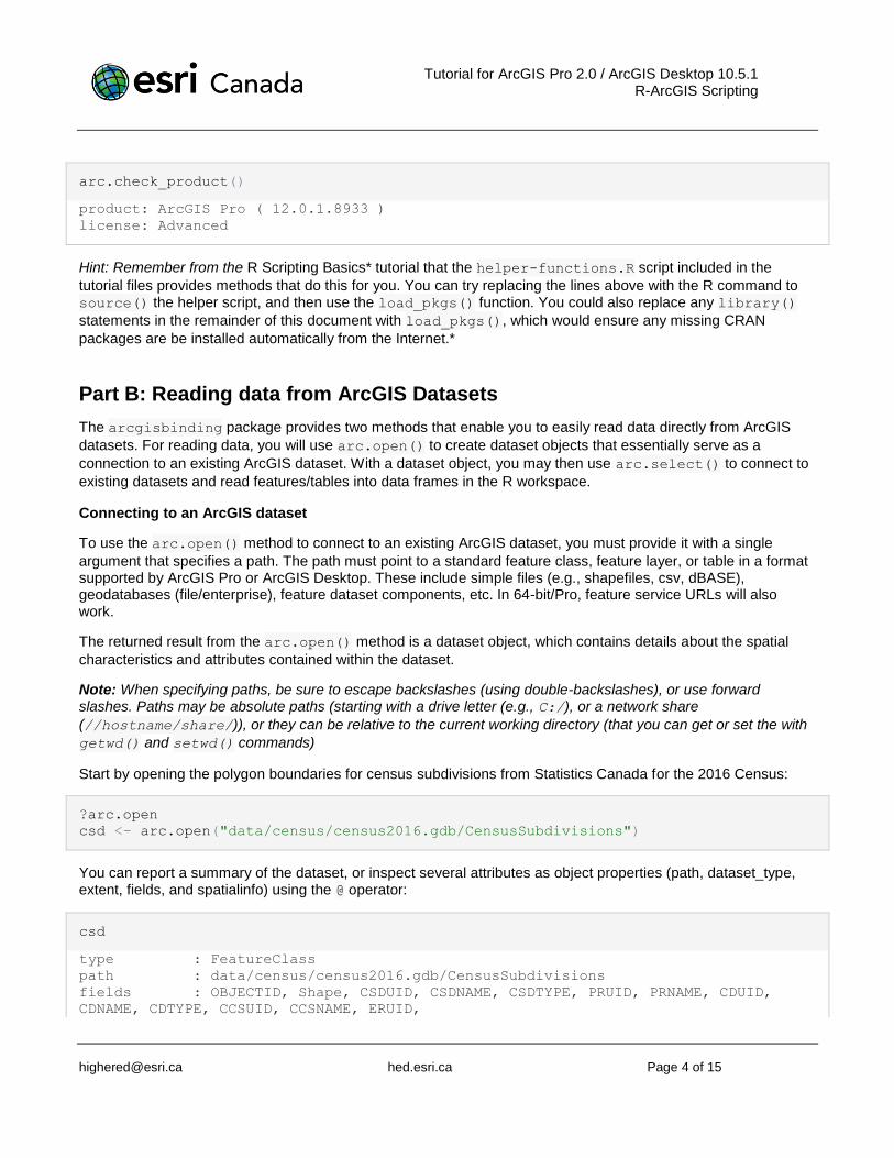
Tutorial for ArcGIS Pro 2.0 / ArcGIS Desktop 10.5.1 R-ArcGIS Scripting

[email protected] hed.esri.ca Page 1 of 15

R-ArcGIS Scripting

Tutorial Overview

R is an open-source statistical computing language that offers a large suite of data analysis and statistical tools, and is currently the de facto standard for statistical data analysis and visualization for academics and other communities. While its various third-party packages introduce a variety of advanced spatial statistical capabilities, it can be a challenge to access many spatial datasets. The R-ArcGIS bridge solves this challenge by providing an arcgisbinding package that allows ArcGIS datasets to be read and written easily from the R programming

language. This tutorial will introduce you to the use of the R-ArcGIS Bridge in R scripts, and enable you to integrate ArcGIS datasets into your R statistical processes. It will also give you have the pre-requisite knowledge to create script tools in ArcGIS that execute R functions, which will be covered in the following tutorial in this series.

Skills

By completing this tutorial, you will become comfortable with the following skills:

• Reading/writing ArcGIS datasets using the arcgisbinding package.

• Working with ArcGIS datasets in R

• Manipulating and analyzing spatial data in R

Time required

The following classroom time is required to complete this tutorial:

• 45 - 60 minutes

Materials Required

• Technology:

– R Statistical Computing Language (version 3.2.0+)

– RStudio Desktop (version 1.0.153+)

– ArcGIS Pro 1.1+ (2.0+ recommended) or ArcGIS Desktop 10.3.1+ (10.5.1+ recommended)

– R-ArcGIS Bindings (1.0.0.128+ recommended)

• Data:

– Data for this tutorial are included as part of the download in the packaged data folder.

Data Sources • City of Toronto:

https://www1.toronto.ca/wps/portal/contentonly?vgnextoid=1a66e03bb8d1e310VgnVCM10000071d60f89RCRD

• Statistics Canada: http://www12.statcan.gc.ca/census-recensement/2016/dp-pd/index-eng.cfm



http://www12.statcan.gc.ca/census-recensement/2016/dp-pd/index-eng.cfm



Production Date

The Education and Research Group at Esri Canada makes every effort to present accurate and reliable information. The Web sites and URLs used in this tutorial are from sources that were current at the time of production, but are subject to change without notice to Esri Canada.

• Production Date: October 2017

Background Information

The R user community has seen substantial growth in recent years, and is expected to continue growing due to the increasing popularity of statistical data analysis. You can use R in conjunction with ArcGIS to develop tools that can broaden the functionality of ArcGIS. Before you can create these tools, you need to develop an understanding of how to work with the arcgisbinding package that is installed by the R-ArcGIS bridge.

Learning how to incorporate ArcGIS datasets into your R scripts to perform data analysis will greatly extend the possibilities that exist for analyzing both spatial and non-spatial data.

R is different from many other programming languages, in that it was developed primarily for data analysis and computational statistics. While the language and environment have evolved over the past two decades to incorporate many other capabilities, this initial focus provides R with almost every statistical model and data manipulation technique that you would need for modern data analysis. However, it can be a challenge to integrate with other data types or software environments.

The arcgisbinding package resolves the challenge of working with ArcGIS datasets by introducing to R a set

of functions and classes that facilitate reading, writing, and manipulating ArcGIS datasets in the R programming language. It further enables integration of R with ArcGIS software through the ability to create script tools in ArcGIS toolboxes that execute R code.

By completing this tutorial, you will become familiar with the use of the arcgisbinding and the capabilities it

introduces to the R environment. You will learn how to read and write data from ArcGIS datasets, and manipulate and analyze spatial data in the R programming language.

References and Reading • R-ArcGIS Bridge: full documentation for the arcgisbinding package

https://r-arcgis.github.io/assets/arcgisbinding.pdf

• R-ArcGIS Bridge: vignette for the arcgisbinding package

https://r-arcgis.github.io/assets/arcgisbinding-vignette.html

• R-Stats group on GeoNet https://geonet.esri.com/groups/rstats

• R Statistical Computing Language http://www.r-project.org/

• Spatial 'view' of packages in the Comprehensive R Archive Network https://cran.r-project.org/web/views/Spatial.html

https://r-arcgis.github.io/assets/arcgisbinding.pdf

https://r-arcgis.github.io/assets/arcgisbinding-vignette.html

https://geonet.esri.com/groups/rstats

http://www.r-project.org/

https://cran.r-project.org/web/views/Spatial.html



Part A: Getting Started

To prepare for this workshop, you should have successfully completed the Getting Started and R Scripting Basics tutorials, which will ensure that you the required software installed and configured, as well as the basic R scripting skills necessary to complete this tutorial. From the R Scripting Basics tutorial, should be familiar with the R and RStudio software, and be able to work with the R Markdown format within the RStudio IDE. In this tutorial, everything discussed can be completed using the default RGui installed with R. However, this document is available as an R-Markdown file that you can open and use interactively in RStudio. If you choose instead to use RGui or another IDE, you can copy/paste code snippets into any R console or R script, or otherwise or adapt the code in another IDE environment.

Setup

To work with the R Markdown source for this document:

1. Open the r-arcgis-rstudio.Rproj file in RStudio

2. Open the File tab in the top-right panel (based on the layout options recommended in the R Scripting Basics tutorial), and click on the file named 3-R-ArcGIS-Scripting.Rmd. The R-Markdown source code for this

document will open in the Source editor window in the top-left.

3. In the top-right corner of the source editor, you may click the maximize icon to toggle the maximized state of the panel, and use as much screen space as possible to display the document's source code.

Note: The remainder of this document is written with the expectation that you are working with the R Markdown file in RStudio. If not, you may manually copy R commands enclosed in the ```{r} code blocks into any R console, provided that your current working directory (reported by getwd()) corresponds with the location where the

tutorial files are located.

Before proceeding to interactively run code in the rest of the R Markdown document, select Restart R and Clear

Output from the menu, and then run the following block to configure the R environment to help with the display of outputs in the resulting R Notebook, and to prepare a data.gdb file geodatabase from an empty

template:

Load the R-ArcGIS arcgisbinding package

In any stand-alone R script, you must load the arcgisbinding package in the current R session, and then call

arc.check_product() before you can use any of the functionality provided by the arcgisbinding package.

In the next tutorial, you will learn that this is not required when using an R script configured as a script tool in an ArcGIS Toolbox. However, it is a step that must always be performed to use arcgisbinding methods from an

R console or in an R IDE such as RStudio.

To get started using the arcgisbinding package in this tutorial, run the block of code below to load the

package and bind to your ArcGIS Pro or ArcGIS Desktop (ArcMap) software in your current R session:

library(arcgisbinding)

*** Please call arc.check_product() to define a desktop license.



arc.check_product()

product: ArcGIS Pro ( 12.0.1.8933 )

license: Advanced

Hint: Remember from the R Scripting Basics* tutorial that the helper-functions.R script included in the

tutorial files provides methods that do this for you. You can try replacing the lines above with the R command to source() the helper script, and then use the load_pkgs() function. You could also replace any library()

statements in the remainder of this document with load_pkgs(), which would ensure any missing CRAN

packages are be installed automatically from the Internet.*

Part B: Reading data from ArcGIS Datasets

The arcgisbinding package provides two methods that enable you to easily read data directly from ArcGIS

datasets. For reading data, you will use arc.open() to create dataset objects that essentially serve as a

connection to an existing ArcGIS dataset. With a dataset object, you may then use arc.select() to connect to

existing datasets and read features/tables into data frames in the R workspace.

Connecting to an ArcGIS dataset

To use the arc.open() method to connect to an existing ArcGIS dataset, you must provide it with a single

argument that specifies a path. The path must point to a standard feature class, feature layer, or table in a format supported by ArcGIS Pro or ArcGIS Desktop. These include simple files (e.g., shapefiles, csv, dBASE), geodatabases (file/enterprise), feature dataset components, etc. In 64-bit/Pro, feature service URLs will also work.

The returned result from the arc.open() method is a dataset object, which contains details about the spatial

characteristics and attributes contained within the dataset.

Note: When specifying paths, be sure to escape backslashes (using double-backslashes), or use forward slashes. Paths may be absolute paths (starting with a drive letter (e.g., C:/), or a network share

(//hostname/share/)), or they can be relative to the current working directory (that you can get or set the with

getwd() and setwd() commands)

Start by opening the polygon boundaries for census subdivisions from Statistics Canada for the 2016 Census:

?arc.open

csd <- arc.open("data/census/census2016.gdb/CensusSubdivisions")

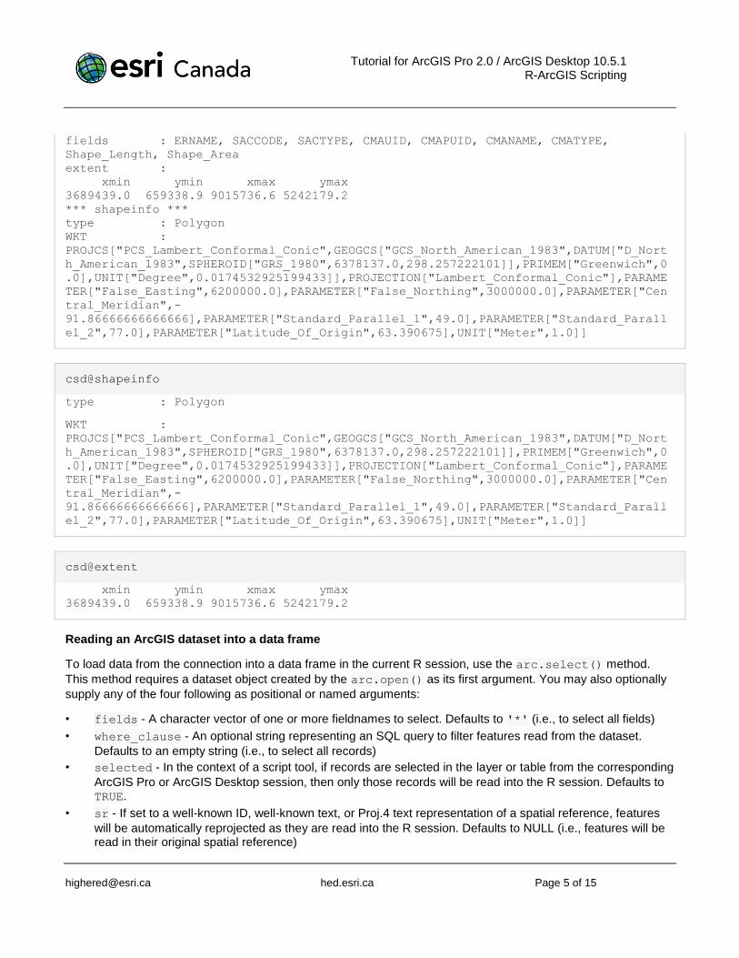
You can report a summary of the dataset, or inspect several attributes as object properties (path, dataset_type, extent, fields, and spatialinfo) using the @ operator:

csd

type : FeatureClass

path : data/census/census2016.gdb/CensusSubdivisions

fields : OBJECTID, Shape, CSDUID, CSDNAME, CSDTYPE, PRUID, PRNAME, CDUID,

CDNAME, CDTYPE, CCSUID, CCSNAME, ERUID,



fields : ERNAME, SACCODE, SACTYPE, CMAUID, CMAPUID, CMANAME, CMATYPE,

Shape_Length, Shape_Area

extent :

xmin ymin xmax ymax

3689439.0 659338.9 9015736.6 5242179.2

*** shapeinfo ***

type : Polygon

WKT :

PROJCS["PCS_Lambert_Conformal_Conic",GEOGCS["GCS_North_American_1983",DATUM["D_Nort

h_American_1983",SPHEROID["GRS_1980",6378137.0,298.257222101]],PRIMEM["Greenwich",0

.0],UNIT["Degree",0.0174532925199433]],PROJECTION["Lambert_Conformal_Conic"],PARAME

TER["False_Easting",6200000.0],PARAMETER["False_Northing",3000000.0],PARAMETER["Cen

tral_Meridian",-

91.86666666666666],PARAMETER["Standard_Parallel_1",49.0],PARAMETER["Standard_Parall

el_2",77.0],PARAMETER["Latitude_Of_Origin",63.390675],UNIT["Meter",1.0]]

csd@shapeinfo

type : Polygon

WKT :

PROJCS["PCS_Lambert_Conformal_Conic",GEOGCS["GCS_North_American_1983",DATUM["D_Nort

h_American_1983",SPHEROID["GRS_1980",6378137.0,298.257222101]],PRIMEM["Greenwich",0

.0],UNIT["Degree",0.0174532925199433]],PROJECTION["Lambert_Conformal_Conic"],PARAME

TER["False_Easting",6200000.0],PARAMETER["False_Northing",3000000.0],PARAMETER["Cen

tral_Meridian",-

91.86666666666666],PARAMETER["Standard_Parallel_1",49.0],PARAMETER["Standard_Parall

el_2",77.0],PARAMETER["Latitude_Of_Origin",63.390675],UNIT["Meter",1.0]]

csd@extent

xmin ymin xmax ymax

3689439.0 659338.9 9015736.6 5242179.2

Reading an ArcGIS dataset into a data frame

To load data from the connection into a data frame in the current R session, use the arc.select() method.

This method requires a dataset object created by the arc.open() as its first argument. You may also optionally

supply any of the four following as positional or named arguments:

• fields - A character vector of one or more fieldnames to select. Defaults to '*' (i.e., to select all fields)

• where_clause - An optional string representing an SQL query to filter features read from the dataset.

Defaults to an empty string (i.e., to select all records)

• selected - In the context of a script tool, if records are selected in the layer or table from the corresponding

ArcGIS Pro or ArcGIS Desktop session, then only those records will be read into the R session. Defaults to TRUE.

• sr - If set to a well-known ID, well-known text, or Proj.4 text representation of a spatial reference, features

will be automatically reprojected as they are read into the R session. Defaults to NULL (i.e., features will be read in their original spatial reference)



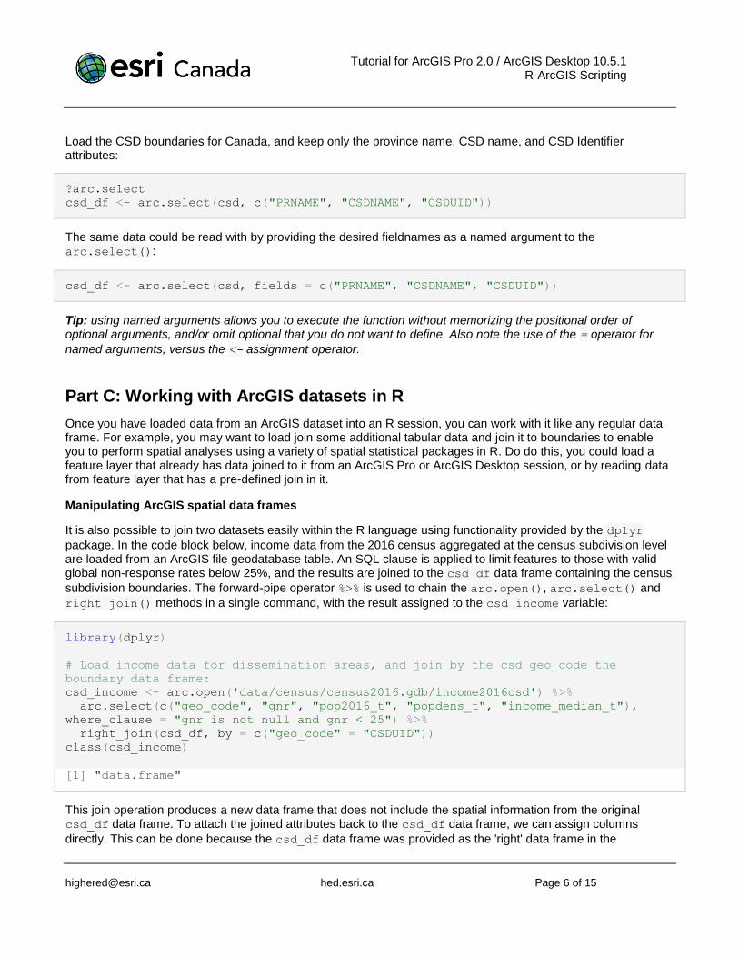
Load the CSD boundaries for Canada, and keep only the province name, CSD name, and CSD Identifier attributes:

?arc.select

csd_df <- arc.select(csd, c("PRNAME", "CSDNAME", "CSDUID"))

The same data could be read with by providing the desired fieldnames as a named argument to the arc.select():

csd_df <- arc.select(csd, fields = c("PRNAME", "CSDNAME", "CSDUID"))

Tip: using named arguments allows you to execute the function without memorizing the positional order of optional arguments, and/or omit optional that you do not want to define. Also note the use of the = operator for

named arguments, versus the <- assignment operator.

Part C: Working with ArcGIS datasets in R

Once you have loaded data from an ArcGIS dataset into an R session, you can work with it like any regular data frame. For example, you may want to load join some additional tabular data and join it to boundaries to enable you to perform spatial analyses using a variety of spatial statistical packages in R. Do do this, you could load a feature layer that already has data joined to it from an ArcGIS Pro or ArcGIS Desktop session, or by reading data from feature layer that has a pre-defined join in it.

Manipulating ArcGIS spatial data frames

It is also possible to join two datasets easily within the R language using functionality provided by the dplyr

package. In the code block below, income data from the 2016 census aggregated at the census subdivision level are loaded from an ArcGIS file geodatabase table. An SQL clause is applied to limit features to those with valid global non-response rates below 25%, and the results are joined to the csd_df data frame containing the census

subdivision boundaries. The forward-pipe operator %>% is used to chain the arc.open(), arc.select() and

right_join() methods in a single command, with the result assigned to the csd_income variable:

library(dplyr)

# Load income data for dissemination areas, and join by the csd geo_code the

boundary data frame:

csd_income <- arc.open('data/census/census2016.gdb/income2016csd') %>%

arc.select(c("geo_code", "gnr", "pop2016_t", "popdens_t", "income_median_t"),

where_clause = "gnr is not null and gnr < 25") %>%

right_join(csd_df, by = c("geo_code" = "CSDUID"))

class(csd_income)

[1] "data.frame"

This join operation produces a new data frame that does not include the spatial information from the original csd_df data frame. To attach the joined attributes back to the csd_df data frame, we can assign columns

directly. This can be done because the csd_df data frame was provided as the 'right' data frame in the



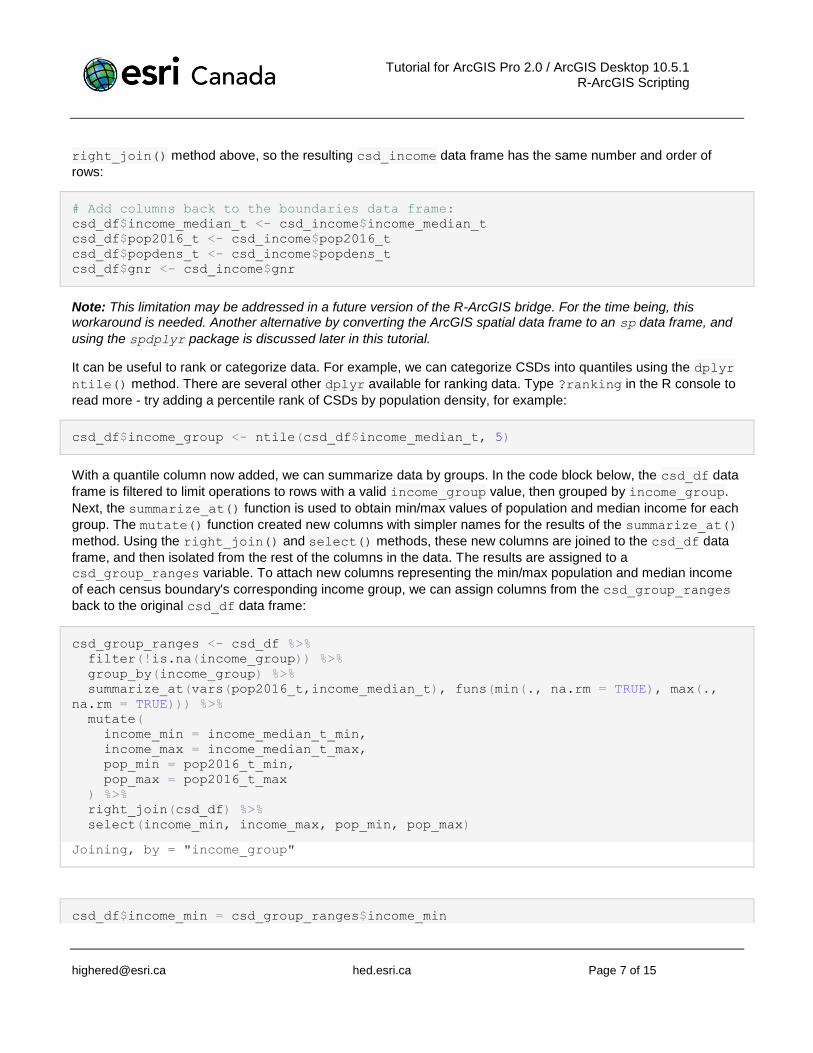
right_join() method above, so the resulting csd_income data frame has the same number and order of

rows:

# Add columns back to the boundaries data frame:

csd_df$income_median_t <- csd_income$income_median_t

csd_df$pop2016_t <- csd_income$pop2016_t

csd_df$popdens_t <- csd_income$popdens_t

csd_df$gnr <- csd_income$gnr

Note: This limitation may be addressed in a future version of the R-ArcGIS bridge. For the time being, this workaround is needed. Another alternative by converting the ArcGIS spatial data frame to an sp data frame, and

using the spdplyr package is discussed later in this tutorial.

It can be useful to rank or categorize data. For example, we can categorize CSDs into quantiles using the dplyr

ntile() method. There are several other dplyr available for ranking data. Type ?ranking in the R console to

read more - try adding a percentile rank of CSDs by population density, for example:

csd_df$income_group <- ntile(csd_df$income_median_t, 5)

With a quantile column now added, we can summarize data by groups. In the code block below, the csd_df data

frame is filtered to limit operations to rows with a valid income_group value, then grouped by income_group.

Next, the summarize_at() function is used to obtain min/max values of population and median income for each

group. The mutate() function created new columns with simpler names for the results of the summarize_at()

method. Using the right_join() and select() methods, these new columns are joined to the csd_df data

frame, and then isolated from the rest of the columns in the data. The results are assigned to a csd_group_ranges variable. To attach new columns representing the min/max population and median income

of each census boundary's corresponding income group, we can assign columns from the csd_group_ranges

back to the original csd_df data frame:

csd_group_ranges <- csd_df %>%

filter(!is.na(income_group)) %>%

group_by(income_group) %>%

summarize_at(vars(pop2016_t,income_median_t), funs(min(., na.rm = TRUE), max(.,

na.rm = TRUE))) %>%

mutate(

income_min = income_median_t_min,

income_max = income_median_t_max,

pop_min = pop2016_t_min,

pop_max = pop2016_t_max

) %>%

right_join(csd_df) %>%

select(income_min, income_max, pop_min, pop_max)

Joining, by = "income_group"

csd_df$income_min = csd_group_ranges$income_min



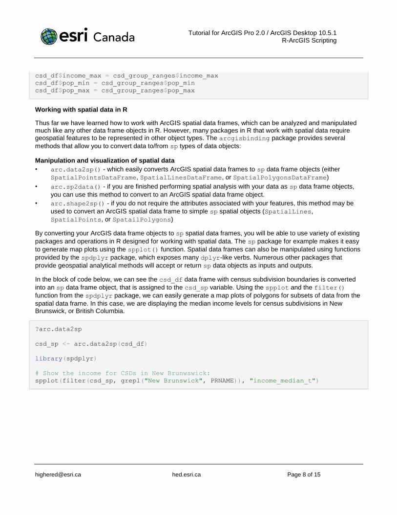
csd_df$income_max = csd_group_ranges$income_max

csd_df$pop_min = csd_group_ranges$pop_min

csd_df$pop_max = csd_group_ranges$pop_max

Working with spatial data in R

Thus far we have learned how to work with ArcGIS spatial data frames, which can be analyzed and manipulated much like any other data frame objects in R. However, many packages in R that work with spatial data require geospatial features to be represented in other object types. The arcgisbinding package provides several

methods that allow you to convert data to/from sp types of data objects:

Manipulation and visualization of spatial data

• arc.data2sp() - which easily converts ArcGIS spatial data frames to sp data frame objects (either

SpatialPointsDataFrame, SpatialLinesDataFrame, or SpatialPolygonsDataFrame)

• arc.sp2data() - if you are finished performing spatial analysis with your data as sp data frame objects,

you can use this method to convert to an ArcGIS spatial data frame object.

• arc.shape2sp() - if you do not require the attributes associated with your features, this method may be

used to convert an ArcGIS spatial data frame to simple sp spatial objects (SpatialLines,

SpatialPoints, or SpatailPolygons)

By converting your ArcGIS data frame objects to sp spatial data frames, you will be able to use variety of existing

packages and operations in R designed for working with spatial data. The sp package for example makes it easy

to generate map plots using the spplot() function. Spatial data frames can also be manipulated using functions

provided by the spdplyr package, which exposes many dplyr-like verbs. Numerous other packages that

provide geospatial analytical methods will accept or return sp data objects as inputs and outputs.

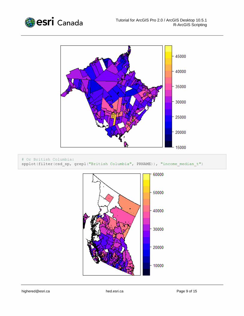
In the block of code below, we can see the csd_df data frame with census subdivision boundaries is converted

into an sp data frame object, that is assigned to the csd_sp variable. Using the spplot and the filter()

function from the spdplyr package, we can easily generate a map plots of polygons for subsets of data from the

spatial data frame. In this case, we are displaying the median income levels for census subdivisions in New Brunswick, or British Columbia.

?arc.data2sp

csd_sp <- arc.data2sp(csd_df)

library(spdplyr)

# Show the income for CSDs in New Brunwswick:

spplot(filter(csd_sp, grepl("New Brunswick", PRNAME)), "income_median_t")



# Or British Columbia:

spplot(filter(csd_sp, grepl("British Columbia", PRNAME)), "income_median_t")



With the spdplyr package available for working with sp data frame objects, we can to perform additional

operations like left_join() or inner_join() and retain the data frame's spatial properties. For example, the

earlier code block that created the csd_income data frame by performing a join with the csd_df data frame

could rewritten as follows:

# Load Saskatchewan boundaries and income data:

sask_df <- arc.select(csd,

fields = c("PRNAME", "CSDNAME", "CSDUID"), where_clause = "PRNAME like 'Sask%'")

income_df <- arc.open('data/census/census2016.gdb/income2016csd') %>%

arc.select(c("geo_code", "gnr", "pop2016_t", "popdens_t",

"income_median_t"), where_clause = "gnr is not null and gnr < 25")

# Join income data to the saskatchewan boundaries using by using an intermediate sp

data frame

csd_income_spatial <- arc.sp2data(left_join(arc.data2sp(sask_df),

income_df, by = c("CSDUID" = "geo_code")))

class(csd_income_spatial)

[1] "tbl_df" "tbl" "data.frame" "arc.data"

The resulting csd_income_spatial data frame created above will have ArcGIS spatial properties, plus the

additional columns added directly to it from the joined data frame. If you inspect it in the Environment tab in RStudio, you will see its first 7 columns are identical to the csd_df that we have been working with so far in this

tutorial.

Because of the intermediate translation to/from an sp data frame, this may be less efficient when working with

larger datasets (e.g., the sample above is limited to Saskatchewan boundaries). If you need to work with your data in sp data frames in your analysis, you can use this approach and other verbs supported by spdplyr to

help simplify your code. You can get full details about the dplyr verbs that can be executed with sp data frames

using the spdplyr package by executing ?"dplyr-Spatial" to display the corresponding help

documentation.

Analyzing spatial data in R

There are many different spatial statistical analysis packages available for R. To get a thorough overview, refer to the Spatial CRAN Task View at https://cran.r-project.org/web/views/Spatial.html. Typically, the spatial analysis functions in each of package will work with specific structures of data, or specific data object types, such as sp

data frames.

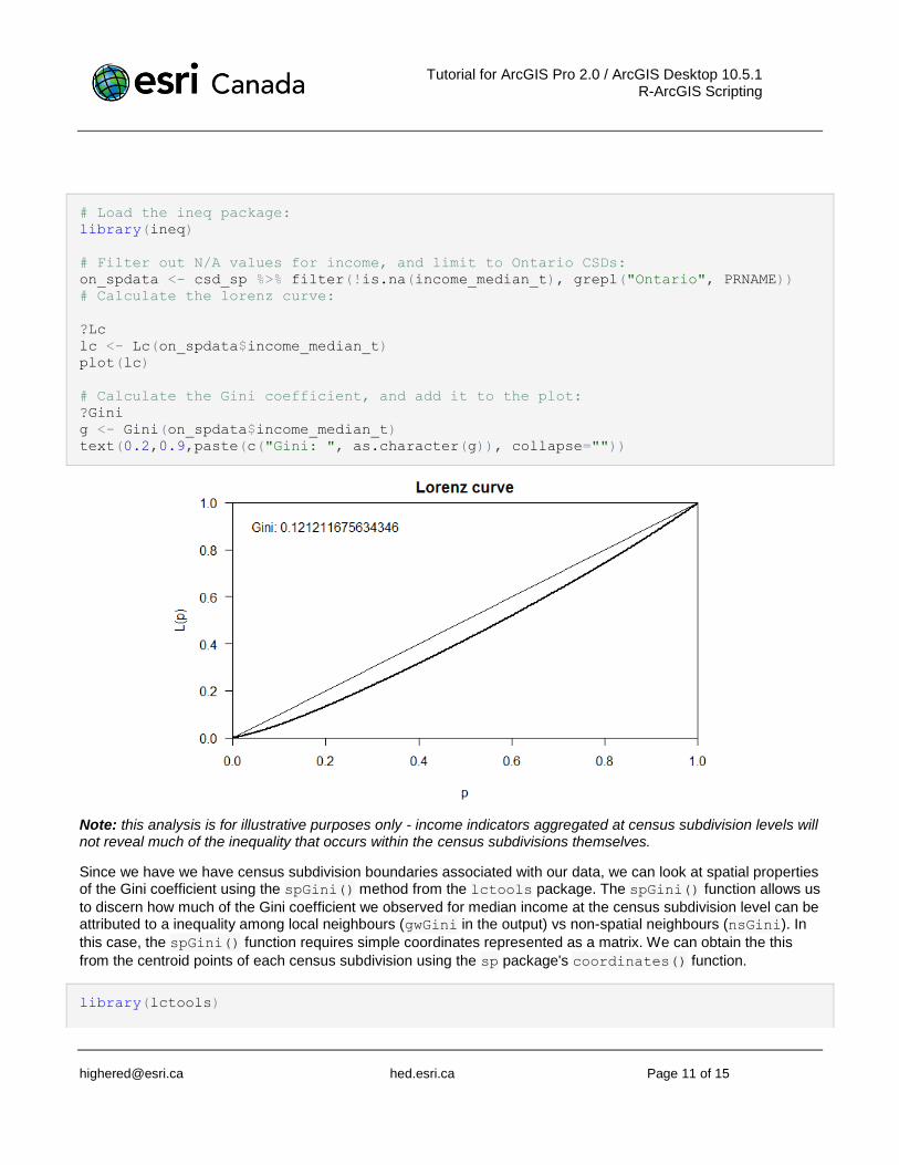
As an example, using the income data available for census subdivisions, we can calculate income inequality statistics using functions provided by the ineq package. In the code block below, we can generate a Lorenz

curve and calculate the Gini coefficient for census subdivisions within Ontario to measure inequality of median income across the province.

Note: the plot() and text() command must be executed at the same time to work properly. When running

these functions within the R-Markdown document in RStudio, either highlight all of the lines from the plot()

command to the text() command and press CTRL+Enter, or run the entire block at once by pressing the

button.

https://cran.r-project.org/web/views/Spatial.html



# Load the ineq package:

library(ineq)

# Filter out N/A values for income, and limit to Ontario CSDs:

on_spdata <- csd_sp %>% filter(!is.na(income_median_t), grepl("Ontario", PRNAME))

# Calculate the lorenz curve:

?Lc

lc <- Lc(on_spdata$income_median_t)

plot(lc)

# Calculate the Gini coefficient, and add it to the plot:

?Gini

g <- Gini(on_spdata$income_median_t)

text(0.2,0.9,paste(c("Gini: ", as.character(g)), collapse=""))

Note: this analysis is for illustrative purposes only - income indicators aggregated at census subdivision levels will not reveal much of the inequality that occurs within the census subdivisions themselves.

Since we have we have census subdivision boundaries associated with our data, we can look at spatial properties of the Gini coefficient using the spGini() method from the lctools package. The spGini() function allows us

to discern how much of the Gini coefficient we observed for median income at the census subdivision level can be attributed to a inequality among local neighbours (gwGini in the output) vs non-spatial neighbours (nsGini). In

this case, the spGini() function requires simple coordinates represented as a matrix. We can obtain the this

from the centroid points of each census subdivision using the sp package's coordinates() function.

library(lctools)



?spGini

?coordinates

# the spGini method relies on simple x/y coordinates:

coords = coordinates(on_spdata)

spG <- spGini(coords, 15, on_spdata$income_median_t)

spG

Gini gwGini nsGini gwGini.frac nsGini.frac

0.12121168 0.00292217 0.11828951 0.02410799 0.97589201

The results of the spGini() analysis in this example will show that the majority of the Gini coefficient for the

province of Ontario at the census subdivision level does not come from inequality between neighbouring locations (with 97.5% of the global Gini coming from inequality between non-spatially coincident census subdivisions). The significance of these results can be tested by running a monte-carlo simulation series using the mc.spGini()

function (Note: this test may take a few minutes to execute):

?mc.spGini

# Run a monte-carlo simulation to test significance:

spG.sim20 <- mc.spGini(Nsim=19, 15, on_spdata$income_median_t, coords[,1],

coords[,2])

spG.sim20$pseudo.p

[1] 0.05

By running 19 (or more) simulations, it can be argued that the observed results from spGini() are significant by

obtaining pseudo p-value of 0.05 or lower (i.e., suggesting that the probability that the observed result is due to chance is 5% or less).

Part D: Writing data from R to ArcGIS datasets

At this point, we have shown that ArcGIS datasets can be read easily into an R session, and demonstrated how you can manipulate spatial data frames, visualize the spatial data in map plots, and use the spatial data objects in spatial analyses. However, the R-ArcGIS bridge works in both directions, enabling you to further analyze, visualize, and collaborate by connecting the outputs of your R programs to the ArcGIS platform.

The simplest approach for this that the arcgisbinding package provides is to write your data to ArcGIS

datasets using the arc.write() method. With this function, you can write spatial and tabular data frames to

conventional ArcGIS dataset formats. The arc.write() method requires at least two arguments:

• path: the full or relative path to an ArcGIS dataset that will be created (*.shp, *.csv, *.dbf, *.gdb

featureclass/table, etc)

• data: the data frame to be written (ArcGIS or sp spatial data frame, or simple tabular data frame). This

must be an ArcGIS spatial data frame, an sp data frame, or a simple tabular data frame.

Optional arguments include:

• coords: list containing geometry information (e.g., to add spatial properties to tabular data)



• shape_info: a list object containing geometry type and spatial reference information

In the code block below, you can see the Ontario census subdivision data we analyzed being converted to an ArcGIS data frame object using the arc.sp2data() function, assigned to the on_dfdata variable name. This

is then written as a new feature class in an a sample data.gdb file geodatabase:

?arc.write

on_dfdata <- arc.sp2data(on_spdata)

arc.write('data.gdb/ontario_data', on_dfdata, shape_info=list(type="Polygon",

WKT=csd@shapeinfo$WKT)

Choosing an output path for arc.write():

When you specify the output path to use with arc.write(), ensure that you appropriately define a new path for

a shapefile inside a regular folder, or to a new featureclass inside of an ArcGIS geodatabase. These paths may be relative, or absolute file locations (as with the arc.open() command), for example:

• arc.write('data.gdb/ontario_data', on_dfdata) - creates a new feature class in an existing

data.gdb file geodatabase

• arc.write('data.sde/ontario_data', on_dfdata) - creates a new feature class in an existing

enterprise geodatabse, identified by the data.sde connection file

• arc.write('data/ontario_data.shp' on_dfdata) - creates a new shapefile in the data folder

location

If you want to save tabular data, specify path to a new table name in a geodatabase, or an appropriate tabular file format in a folder. If the dataset you are saving is in an ArcGIS spatial data frame, and you only want to save the tabular data, you can wrap the variable in the data.frame() function to discard the spatial information. For

example:

• arc.write('data.gdb/ontario_data_tbl', data.frame(on_dfdata)) - creates a new table in

an existing data.gdb file geodatabase

• arc.write('data/ontario_data_tbl.dbf', data.frame(on_dfdata) - creates a new table in

dBASE format in the data folder

• arc.write('data/ontario_data_tbl.csv' data.frame(on_dfdata)) - creates a new table in

comma-separated variable text format in the data folder

Note: fieldnames in feature classes and tables will be truncated when written to shapefile or dBASE formats. When written to geodatabases, invalid characters in fieldnames will be converted to underscores, and fieldnames may otherwise be converted to upper or lowercase depending on the underlying database system.

It is important also to be aware that the arc.write() method from the arcgisbinding package does not

currently support overwriting existing datasets. For example, if you run the sample code block above twice, it will report an error the second time because the ontario_data feature class already exists in the output data.gdb

file geodatabase. You can handle this when running standalone R scripts in one of two ways:

• Use a unique output path/filename each time you use arc.write() (e.g., by using the tempfile()

method in the R base)



• Delete any output dataset at a given path before using the same path with arc.write(). With this

approach, you can use the base R file manipulation functions (see ?files for details) to delete simple

file/folder paths. However, for ArcGIS geodatabases (either file or enterprise), ArcGIS software (or perhaps a Python script using ArcPy commands) must be used to delete or move datasets.

When an R script is run as a script tool in an ArcGIS Toolbox, overwriting output files is less of a concern when the paths are defined using output parameters. In this context, the ArcGIS geoprocessing environment will either prevent overwriting existing datasets, or cleanly remove them before executing the script tool (based on whether the geoprocessing option to allow tools to overwrite outputs is enabled).

Defining the spatial_info parameter

You will typically only need to supply two parameters in the list object supplied in the shape_info parameter for

the arc.write() function:

• type - the geometry type, either "Point", "Polyine", "Polygon"

• WKT - the Well-known text representation of the dataset's spatial reference system

If you are writing data that have the same shape type and projection as an ArcGIS dataset object created by the arc.open() command, then you can pass the @shapeinfo property of the dataset object directly as the

shape_info parameter for the arc.write() command. In the earlier codeblock, the data that were written to

the data.gdb/ontario_data feature class have the same geometry type and same spatial reference system

as the csd data object. Thus the arc.write() command would achieve the same by supplying

csd@shapeinfo as the value for the shape_info argument instead of defining a new list() object.

Working with spatial reference definitions:

In some cases, depending on your specific data source and/or the process through which your data are created, you may need to use different representations of spatial reference systems. The arcgisbinding package

provides two convenience methods for converting between Well-known ID / Well-known Text and Proj.4 spatial reference systems definitions:

• arc.fromWktToP4() - converts a Well-known ID or Well-known Text spatial reference to Proj.4 text

• arc.fromP4ToWkt() - converts a Proj.4 spatial reference text string to Well-known text format. You may

use '+init=epsg:' (in ArcGIS Pro only) to convert spatial references from EPSG identifiers to WKT.

Note: these functions are fully-functional only when executed in ArcGIS Pro as a script tool. You can experiment with them more in the context of a script tool executed from ArcGIS Pro, after completing the next tutorial.

Exercise 1

At this point, you are now able to read, manipulate, analyze, visualize, and write ArcGIS datasets in the R programming language using the arcgisbinding package installed by the R-ArcGIS bridge. To test your skills,

try the following:

• Read the 'data/toronto/neighbourhoods_crime.shp' shapefile into a new spatial data frame

• Load the 'data/toronto/wb_civics_2011.csv' table into a new data frame, and join its columns to the neighbourhoods_crime data frame. Hint: one of these stores its identifier as a character vector

• Add a column with quantile ranks, group/summarize some of the data, create some box plots.



• Write the data with the columns added from the wb_civics_2011.csv data back to a new shapefile. Hint: remember the result of a join using dplyr with an ArcGIS spatial data frame does not return shape data – copy columns back to the original data frame created by the arc.select() command, or use an intermediate sp data frame.

• Add the new shapefile to your map in ArcGIS Pro or ArcMap, and style it by the quantile ranks you added.

Future Considerations

The arcgisbinding package provided by the R-ArcGIS bridge is an effective tool to integrate ArcGIS datasets

efficiently into your R programs. It also allows you to generate new ArcGIS datasets as outputs from your R programs to make results from your analyses easily viewed and processed in ArcGIS applications. This is a significant advantage for developing R programs that need to work with spatial datasets that are easily managed by ArcGIS applications.

Integration of your R scripts with the ArcGIS platform is even more effective if you implement them as script tools in an ArcGIS toolbox. Doing so makes input/output of datasets and numerical/text parameter values seamless, and enables immediate visualization of feature classes and tables output by your tools. Your R script tools can be further integrated into larger processes, for example by incorporating them into an ArcGIS Model Builder workspace to create more advanced geoprocessing workflows.

It is highly recommended that you continue the tutorial series by completing the Building R Script Tools tutorial. This will teach you how to create toolboxes that integrate your R code with ArcGIS Pro or ArcGIS Desktop.

http://hed.esri.ca

© 2017 Esri Canada. All rights reserved. Trademarks provided under license from Environmental Systems Research Institute Inc. Other product and company names mentioned herein may be trademarks or registered trademarks of their respective owners. Errors and omissions excepted. This work is licensed under a Creative Commons Attribution-NonCommercial-ShareAlike 4.0 International License.

http://hed.esri.ca/

http://creativecommons.org/licenses/by-nc-sa/4.0/

http://creativecommons.org/licenses/by-nc-sa/4.0/

Documents

R-ArcGIS Scripting - esricanada-ce.github.io · Tutorial for ArcGIS Pro 2.0 / ArcGIS Desktop 10.5.1 R-ArcGIS Scripting [email protected] hed.esri.ca Page 1 of 15 R-ArcGIS Scripting