Racial Segregation and Public SchoolExpenditure∗

Eliana La Ferrara

Bocconi Universityand IGIER

Angelo Mele

University of Illinoisat Urbana-Champaign

This version: October 2005

Abstract

This paper explores the effect of racial segregation on public schoolexpenditure in US metropolitan areas and school districts. Greatersegregation is associated with more homogeneity in some sub-areasand more heterogeneity in others, so the overall effect is ambiguous.We find that after accounting for the potential endogeneity of racialsegregation in metropolitan areas, the latter has a positive impacton public school expenditure both at the MSA and at the districtlevel. At the same time, we find that increased segregation leads tomore inequality in spending across districts of the same MSA, thusworsening the relative position of poorer districts.

Keywords: segregation, racial fragmentation, public school expen-diture

∗We are grateful to Caroline Hoxby for very helpful discussions. We also benefited fromcomments by Emanuela Galasso, Steve Ross, and by seminar participants in the CEPR PPSymposium-La Coruna and at Bocconi University. David Aultman kindly provided someof the data. The usual disclaimer applies. Correspondence: eliana.laferrara@unibocconi.it;angelo.mele@uiuc.edu.

1

1 Introduction

The existence of sizeable differences among US school districts in public ed-ucation expenditure is a well known fact. Several studies have shown howspending per pupil can vary by a factor of two or more between contigu-ous jurisdictions within the same state, and the proportion of such spend-ing funded through local taxes can vary by as much as a factor of four.1

A variety of demographic and economic characteristics of the jurisdictionshave been shown to correlate significantly with spending levels, e.g. averagehousehold income, mean property values, racial fragmentation, the fractionof people aged 65 and above, etc. Predictions consistent with such findingscan be derived from existing multicommunity models that embody propor-tional income or property taxation, differing qualities of public education,peer effects, and differences in human capital endowments and/or tastes foreducation among races. Surprisingly, one important feature of US commu-nities has been overlooked in empirical studies of the determinants of publiceducation expenditure: residential segregation among races. Assessing theimpact of segregation on public education expenditure is important for atleast two reasons: first, to get a more complete picture of what explains dif-ferences in spending levels across jurisdictions; second, to add yet another(possibly undesirable) effect of segregation on individual outcomes, this timemeasured through a crucial input into economic success, namely access toaffordable education.We can think of two ways in which segregation may affect education

expenditure. The first operates through a simple “aggregation” effect. Dif-ferent degrees of segregation in a community are associated with differentlevels of fragmentation in the sub-areas that compose that community. Ifwe believe that fragmentation affects willingness and/or ability to spend onlocal public goods, then every time we estimate the determinants of expen-diture levels using data which has a higher level of geographical aggregationthan the level at which decisions are taken and/or interaction occurs, weshould find that segregation plays a significant role. Notice that according to

1Among others, Fernandez and Rogerson (1996), compare total spending per studentin 1986/87 among school districts in the areas of Detroit, New York, and New Jersey.As an example of disparities in local funding levels, Evans, Murray and Schwab (1997)report that in 1987 in Kentucky the district of Whitley County was collecting only $247per student (in 1992 prices) through local taxes, while Walton Verona was collecting asmuch as $1010.

2

this explanation the effect of segregation should disappear once we controldirectly for the composition of the relevant sub-units. The second channelposits that, apart from possible aggregation effect, segregation may have animpact on expenditure due to externalities among the sub-areas that com-pose a community. For example, the extent of competition among schooldistricts within a metropolitan area may depend not only on their number,but also on the characteristics of the available “menu”, e.g. in terms of racialcomposition. In this sense, the degree of segregation of a metropolitan area(MSA) tells us more than the fragmentation indexes of the MSA as a wholeor of the single districts, and can be found to have an independent effect evenafter controlling for the characteristics of each sub-area, precisely because itcaptures the “interdependency”.Using cross sectional data at the MSA and school district level for the

US in 1990, we take into account potential endogeneity by looking at thehistorical determinants of segregation. In particular, we instrument MSA-level racial segregation in 1990 with the share of immigrants into that MSAin 1940 that were "minority". We find that after controlling for racial frag-mentation and for other MSA and district characteristics, racial segregationhas a positive and significant impact on per pupil expenditure. Accordingto our most conservative estimates, the effect of a one standard deviationincrease in segregation is a 10% increase in average per pupil expenditureat the MSA level. With district level data, ceteris paribus, a one standarddeviation increase in the segregation of the MSA where the district is locatedwould increase per pupil expenditure in the district by 20-22 percent. At thesame time, segregation significantly increases inequality in per pupil expen-diture among districts in the same MSA, as measured by a Gini coefficient inschool spending across districts of the same MSA, by the ratio of spendingof the “top” to the “bottom” district, and by the standard deviation of perpupil spending by different districts in the same MSA. In other words, view-ing segregation as a mechanism for sorting into relatively more homogeneousschool districts and school attendance areas, we find that average expendi-ture at the MSA level increases but at the expense of widening disparitiesamong "poor" and "rich" districts.

The remainder of the paper is organized as follows. Section 2 brieflyreviews the literature to which this paper is related and the following sectionsketches some arguments for why segregation can affect expenditure on publiceducation. Section 4 presents the empirical strategy and the data used in this

3

paper and section 5 reports our main econometric results. Finally, Section 6briefly concludes.

2 Background literature

This paper is related to several strands of the literature. First of all, it buildson existing work on the empirical determinants of spending on public edu-cation in the US. Early contributions in this area are surveyed by Rubinfeldand Shapiro (1989) and by Cutler, Elmedorf and Zeckhauser (1993). Morerecent work on school expenditure at the state level includes Poterba (1996)and Fernandez and Rogerson (1997). The first paper uses panel data overthe period 1960-90 and finds that government per child spending on K-12education decreases with the fraction of the population aged 65 and above.This effect is strengthened when the difference between the fraction of non-white population aged 5-17 and the fraction nonwhite aged 65+ is includedamong the controls, suggesting an interplay of demographic and racial com-position effects. On the other hand, the share of nonwhites in the populationper se is never statistically significant. The paper by Fernandez and Roger-son (1997) employs a panel of US states from 1950 to 1990 to estimate howper student spending on public primary and secondary education respondsto changes in income and to demographic characteristics (with no accountfor racial composition), and finds that the share of school aged populationis insignificant, while that of elderly people has a negative effect. Card andPayne (2002) study the impact of school finance reforms in the 1980s on thegap in school spending between rich and poor districts. Alesina, Baqir andEasterly (1999) find that across US counties and metropolitan areas racialfragmentation has a negative and significant impact on local public goodprovision, including public education. In a well known study, Hoxby (2000)estimates the determinants of per pupil spending across school districts as afunction of district and MSA characteristics, including an index of Tieboutchoice, and finds that ceteris paribus spending is lower in areas where thereis more choice among districts, plausibly due to cost saving incentives relatedto competition. Racial heterogeneity of the metropolitan area is also foundto have a negative effect on spending.2 Exploiting variation in the number of

2In a recent study, Rothstein (2005) replicates Hoxby’s analysis and fails to find arobust and significant effect of school choice on school productivity. On the other hand,he does no report results for per pupil expenditure (which is the dependent variable in

4

districts between primary and secondary educational levels within metropoli-tan areas, Urquiola (1999) finds that greater district availability is associatedwith greater expenditure, consistently with a Tiebout-style sorting story. Asstated in the introduction, none of the above papers explicitly considers thegeographic distribution of races across districts or within parts of the samedistrict as an explanatory factor. The present paper attempts to bridge thisgap.A second strand of the literature related to this work is the empirical

literature on the effects of residential segregation on economic outcomes. Thislarge body of studies encompasses tests of the spatial mismatch hypothesis(see Kain (1992) for a survey), and work on neighborhood effects (e.g., Caseand Katz (1991), Borjas (1994)). As forcefully argued by Wilson (1987), on apriori grounds it is not clear that more segregation should necessarily worseneconomic outcomes for the minority. An important study by Cutler andGlaeser (1997) estimates the effect of residential segregation in metropolitanareas (measured by the dissimilarity index) on three kinds of socioeconomicoutcomes: education (i.e., high school and college graduation rates), income(i.e., job idleness and earnings), and single motherhood. In all cases they findthat increased segregation significantly worsens these outcomes at the MSAlevel, also when allowing for endogenous residential location. In a recentstudy, Card and Rothstein (2005) study the effects of school and residentialsegregation on black relative test scores. Exploiting variation in segregationinduced by court-ordered desegregation policies or by the geography of a city,they find that the bulk of the (negative) effect on test scores is attributable toresidential segregation. Guryan (2004) estimates the effect of a desegregationprogram implemented in the 1970 and finds that it led to a 3 percentage pointreduction in the Black-White dropout rate differential. Our paper takesone step back and considers an input which is potentially key to the schoolperformance and to the economic success of the disadvantaged, namely theprovision of public education. In addition to the impact related to spatialmismatch or peer group effects, in fact, it is conceivable that segregationmay affect the ability and/or willingness to provide a local public good suchas public education, and if this were the case the effect of public educationcould reinforce or mitigate the workings of the above channels.Recent contributions by Clotfelter (2004) and by Lankford and Wyckoff

our empirical analysis), nor on the role played by the racial composition of the community(which is the focus of our paper).

5

(2000) have called attention on changing patterns in the racial compositionof schools. The former author constructs measures of school segregationfor the past five decades and finds that, while segregation within districtsdeclined, racial imbalances between districts tended to increase. Lankford andWyckoff (2000), on the other hand, use Census data for eight metropolitanareas in upstate New York and find the racial composition of students issignificantly correlated with parents’ decisions regarding school choice andresidential location. While controlling for racial composition and segregationat smaller geographical levels, our analysis will mainly focus on the effects ofMSA level segregation, as the latter can be instrumented so as to allow anestimate of the causal link going from segregation to expenditure decisions.3

Finally, indirectly related to the present analysis is the recent literature onendogenous jurisdiction formation, notably the papers by Martinez-Vazquez,Rider and Walker (1997), and by Alesina, Baqir and Hoxby (2001). Bothpapers allow for the number of jurisdictions to be determined by the tastefor association with individuals of a similar race, as well as by other factors.Racial heterogeneity is shown to increase the number of school districts,consistently with the hypotheses of these models. In particular, Alesina etal. (2001) show that their result holds both when the dependent variableis the number of school districts in a county, and when it is the number ofschools in a district, i.e. when heterogeneity is allowed to induce sortingwithin jurisdictions. While the present paper will only marginally touch onthe issue of endogenous jurisdiction formation, it will explore the role ofbetween and within-jurisdiction heterogeneity by focusing on the geographicdistribution of races.

3 Racial fragmentation, segregation and schoolspending

There are several channels through which racial segregation can influence lo-cal spending decisions on public education. The first is related to preferencesfor intra-racial interactions (see e.g., Alesina, Baqir and Easterly (1999) andAlesina and La Ferrara (2000)). The model of Alesina, Baqir and Easterlypredicts that when races differ in their preferred type of local public good,

3In recent work, Burgess, Wilson and Lupton (2004) compare the patterns of schooland residential segregation of different ethnic groups in the UK.

6

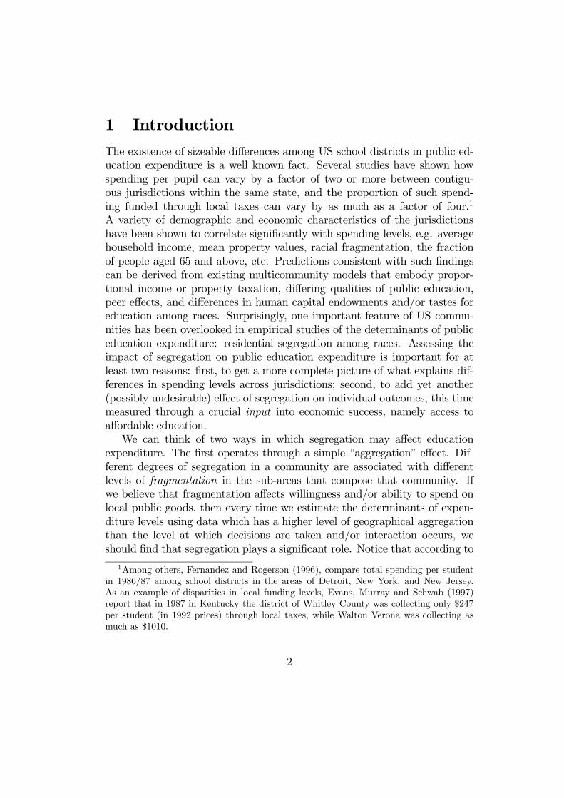
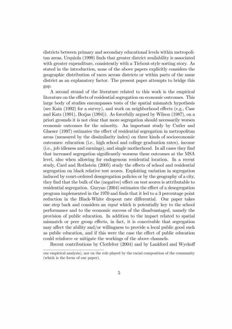
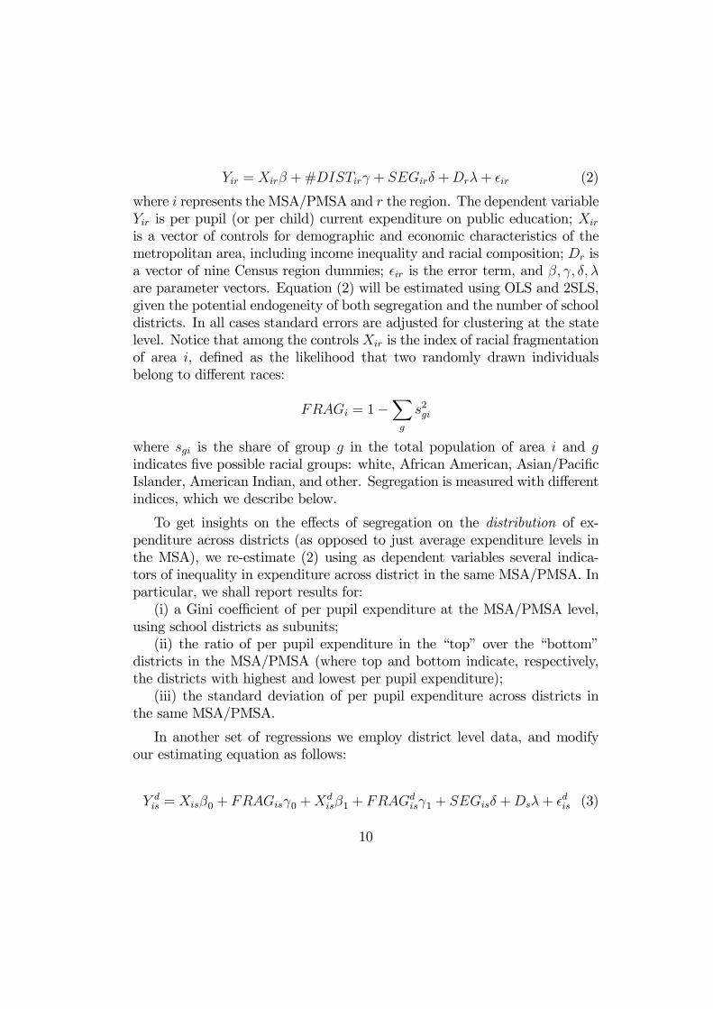
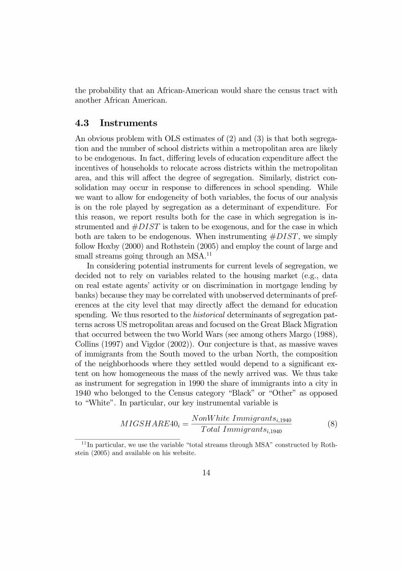
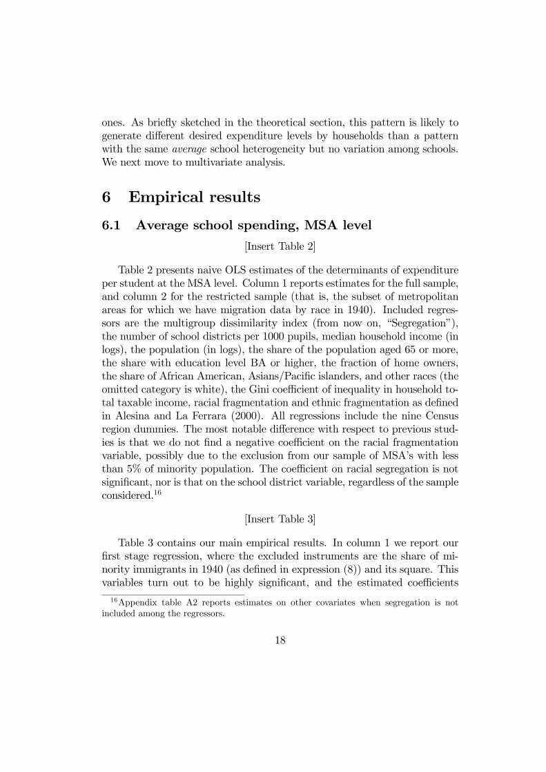
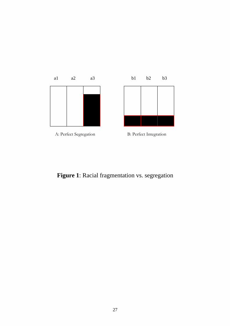
spending on such goods will decline with the degree of racial fragmentation inthe relevant area. In this case segregation can give the opportunities to homo-geneous group to provide their preferred public good at a smaller geographiclevel. Basically, we can expect segregation to have an impact on spendingdecisions depending on the level of aggregation of the data. Consider as anexample figure 1.

[Insert figure 1 here]

Two communities A and B (say, two MSAs) are represented in the fig-ure. Each of them is divided into three smaller units (say, school districts).Different colors in the figure represent different races, with the majority typebeing represented as white and the minority as black. Communities A andB are assumed to have the same population and the same ratio of black towhite population, i.e. the same level of racial fragmentation. However, theydiffer in the degree of racial segregation, which is maximum in communityA and minimum in community B. According to the basic model of Alesina,Baqir and Easterly (1999) the two communities should have the same levelof spending on public education because they have the same fragmentation.However, suppose that the relevant geographic unit for decisions regardingsome local public goods is smaller than the community as a whole, i.e. thateach sub-community can have its own type and level of public good. In thecase of education, this amounts to saying that decisions pertain to schooldistricts and not to metropolitan areas.4 We should then expect A and B toreach different outcomes due to the different levels of within-district fragmen-tation. In particular sub-communities a1 and a2 in the figure will now spendmore than b1 and b2, because they are more homogeneous; a3 will insteadspend less than b3, unless the mass of the minority type is large enough toactually decrease racial fragmentation. The aggregate effect of segregationon MSA-level spending is thus ambiguous. Notice that the same reasoningcan apply at smaller geographic level, e.g. considering A and B as school dis-tricts and the sub-units as school attendance areas. In all cases what mattersis whether the possibility of sorting into more or less homogeneous sub-unitsfor given level of aggregate fragmentation increases or decreases aggregatespending levels.

4Of course, the scheme in the figure is oversimplified because in reality school districtscan extend beyond the borders of metropolitan areas. We will address this issue in theempirical section.

7

A second channel through which segregation may affect spending on pub-lic education is through differences in income. Starting from the work ofEpple, Filimon and Romer (1984) and of Massey and Denton (1993), we canthink of a framework in which the minority type is relatively poorer and thusdifferent degrees of racial segregation imply different levels of income and ofinequality within smaller areas. In terms of figure 2, mean income is higherin a1 and a2 than in b1 and b2, and it is lower in a3 than in b3. Consideringthat education is a normal good, the aggregate effect is once again ambiguousand depends among other factors on the income elasticity of the demand foreducation.5

A third mechanism linking segregation and local school expenditure buildson “social capital” or human capital externalities, along the lines of De Bar-tolome (1990) and Benabou (1996). In Benabou’s model, for example, chil-dren’s human capital is a function of their parents’ human capital, of schoolspending in their community, and of the quality of local interactions L, whichis increasing in the local distribution of human capital. The social capitalvariable L captures local spillovers related to peer effects, network external-ities, and the like. In this setting, when the minority type has lower humancapital endowment, segregation implies higher social capital in some sub-areas and lower in others. In figure 2, a1 and a2 should have more socialcapital than b1 and b2, while a3 should have less than b3. The aggregateeffect will depend on whether the two types are complements or substitutesin the production of social capital and on their degree of complementarity orsubstitutability. Let wi denote the share of whites in each geographic uniti, and let hB and hW denote the human capital endowments of blacks andwhites, respectively. For example, if we adopt a CES formulation for thesocial capital production function, i.e.

Li = [wi(hW )σ + (1− wi)(hB)

σ]1/σ (1)

then depending on other parameter values Benabou’s model can be solved toshow that there is a threshold value eσ such that segregation has a negative(positive) effect on expenditure for σ > (<)eσ.In reality, we are likely to observe a mixture of all these three channels

at work, and they can actually interact in interesting ways. A recent paperby Sethi and Somanathan (2004), for example, argues that it is important

5A caveat on this simple reasoning is that as income increases people may switch toprivate as opposed to public education, but we shall neglect this possibility here.

8

to consider the interplay between preferences on inter-racial interactions andincome differentials between races. Their framework is not applied to theprovision of public education, but an extension in that direction seems im-portant for future work. For present purposes, it should be recognized thatall three channels have in common one feature: segregation can be analyzed asa change in the fragmentation of smaller sub-areas and, through the impactof fragmentation on spending in each sub-area, segregation will affect aggre-gate levels of spending in a nontrivial way. The magnitude and direction ofthe effect depends both on the mechanism of the underlying model and onthe level of geographic aggregation chosen.All the above explanations rely on what we have called “aggregation”

effect, in that community wide segregation only acts through the fact thatit maps into different levels of fragmentation in the sub-areas that composethat community. A different approach, which we referred to as the “exter-nality channel” in the introduction, can be formulated by enriching existingmodels of inter-jurisdictional competition to account for racial composition.While in fact existing models of Tiebout competition posit that the “price” ofeducational services should be a negative function of the number of availabledistricts, it is conceivable that the degree of competition also depends on the“attractiveness” of such districts, and that the racial mix of the districts isone of the features that determine how attractive they are. If this is the case,expenditure in a given district will depend not only on its own racial com-position but also on other districts’ racial composition, and more generallyon the geographic distribution of races in the metropolitan area. Dependingon whether greater segregation increases or decreases effective competitionamong districts, we can expect a decrease or an increase in public schoolexpenditure.6

4 Empirical strategy

4.1 Estimating equations

Our basic estimating equation can be specified as follows:

6Notice that while segregation is endogenous to residential location decisions and isitself a function of inter district competition, in the empirical section we will try to identifythe “exogenous” menu of segregation areas by using instruments that transcend individualdecisions and capture historical patterns of migration by minorities.

9

Yir = Xirβ +#DISTirγ + SEGirδ +Drλ+ ir (2)

where i represents the MSA/PMSA and r the region. The dependent variableYir is per pupil (or per child) current expenditure on public education; Xir

is a vector of controls for demographic and economic characteristics of themetropolitan area, including income inequality and racial composition; Dr isa vector of nine Census region dummies; ir is the error term, and β, γ, δ, λare parameter vectors. Equation (2) will be estimated using OLS and 2SLS,given the potential endogeneity of both segregation and the number of schooldistricts. In all cases standard errors are adjusted for clustering at the statelevel. Notice that among the controls Xir is the index of racial fragmentationof area i, defined as the likelihood that two randomly drawn individualsbelong to different races:

FRAGi = 1−Xg

s2gi

where sgi is the share of group g in the total population of area i and gindicates five possible racial groups: white, African American, Asian/PacificIslander, American Indian, and other. Segregation is measured with differentindices, which we describe below.

To get insights on the effects of segregation on the distribution of ex-penditure across districts (as opposed to just average expenditure levels inthe MSA), we re-estimate (2) using as dependent variables several indica-tors of inequality in expenditure across district in the same MSA/PMSA. Inparticular, we shall report results for:(i) a Gini coefficient of per pupil expenditure at the MSA/PMSA level,

using school districts as subunits;(ii) the ratio of per pupil expenditure in the “top” over the “bottom”

districts in the MSA/PMSA (where top and bottom indicate, respectively,the districts with highest and lowest per pupil expenditure);(iii) the standard deviation of per pupil expenditure across districts in

the same MSA/PMSA.

In another set of regressions we employ district level data, and modifyour estimating equation as follows:

Y dis = Xisβ0 + FRAGisγ0 +Xd

isβ1 + FRAGdisγ1 + SEGisδ +Dsλ+

dis (3)

10

where d represents a school district, i a metropolitan area, and s a State.This specification includes a full set of demographic controls both at the MSAand at the district level, but the coefficients on district level variables can-not be given a structural interpretation due to endogenous Tiebout sorting.Following Hoxby (2000), we will therefore include them to improve the fit ofthe equation, but will not discuss them in the results section. Our focus ison estimating the impact of segregation in the metropolitan area on districtlevel expenditure. Provided that the MSA can be considered as the exoge-nous educational market that households face in their decisions, and that wefind suitable instruments for segregation at the MSA level, we should obtainan unbiased estimate of the coefficient δ.7

Finally, even within the same district a given level of MSA segregationand district fragmentation does not mean that households do not have thepossibility to send their children to more or less homogeneous schools. Thelast part of our district level results augments the specification of (3) with thenumber of schools in the district and with indicators of school compositionwithin the district. Again, while we will not interpret the coefficients onthese variables in a causal way, their inclusion will shed some light on therole played by MSA level segregation in education expenditure decisions.

4.2 Measures of racial segregation

Our baseline specification measures segregation with the multigroup versionof the dissimilarity index, as proposed by Reardon and Firebaugh (2002)

MSEG =MXm=1

nXi=1

Pi

2PI|sim − sm| (4)

where m is the index for race, i indicates the census tract, Pi is the numberof individuals in census tract i, P is the total population of the metropolitanarea, sim is the share of race m in census tract i, and sm is the share of race

7Notice that we have computed segregation also within districts using block level Censusdata, and we will comment on some descriptive statistics ragarding district level segrega-tion. However, we will not include this variable in our regressions due to the unavailabilityof instruments for segregation within districts. For example, Alesina, Baqir and Hoxby(2001) include the number of larger and smaller streams among the explanatory variablesfor the number of school districts in a county, but not for the number of schools within adistrict, because the stream variables are not available at the district level.

11

m in the total population. The index I in the denominator is the SimpsonInteraction Index, a measure of diversity given by the following formula:

I =MX

m=1

sm (1− sm)

This is nothing but the racial fragmentation of the metropolitan area.8 In-tuitively, the multigroup dissimilarity index (4) is a measure of dispropor-tionality of races across the census tracts, and captures the proportion ofall individuals that should transfer among census tracts in order to equalizethe proportion of races across tracts, divided by the proportion that wouldhave to change census tract if the metropolitan area was perfectly segre-gated.9 The index varies between 0 and 1, where zero corresponds to perfectintegration and 1 to perfect segregation.We prefer to rely on a multigroup index to account for the complex racial

heterogeneity patterns of US metropolitan areas In fact, one drawback ofdichotomous indices is that cannot accurately take into account complex seg-regation patterns among all racial groups, since they measure the residentialseparation of a minority group with respect to the rest of the population. Forexample, a dichotomous index measuring the residential segregation of blackswith respect to nonblacks, considers whites, Hispanics and Asians togetheras an homogenous group, while there are clear segregation patterns amongthese racial groups. A multigroup index measures the extent of all thesepatterns separately for each group, while giving a synthetic information.Nonetheless, we also test for robustness of our findings by employing the

standard dichotomic version of the dissimilarity index, i.e. with M = 2,which is the same proposed by Cutler and Glaeser (1997):

8Indeed the Simpson Interaction Index and the Racial Fragmentation Index are thesameI =

PMm=1 sm (1− sm) = 1−

PMm=1 s

2m.

9Rearranging the terms of the multigroup dissimilarity we get MSEG =12I

PMm=1 sm

Pni=1

PiP

¯̄̄simsm− 1¯̄̄. In essence when the metropolitan area is perfectly inte-

grated, every census tract contains the same proportion of each race as in the metrpopoli-tan area as a whole, i.e. sim = sm for all i and all m. The case of perfect integrationimplies an index of zero, since the term in the absolute value is always zero. Wheneverthis equality does not hold the term in the absolute value becomes positive and the indexincreases. So we can interpret this index as the average disproportionality across censustracts, weighted by the race proportions and the population shares.

12

SEG =1

2

Xi

¯̄̄̄Bi

B− NBi

NB

¯̄̄̄(5)

where i indicates census tracts within a metropolitan area, B is the totalnumber of Blacks in that area, Bi is the number of Blacks in census tract i,andNB stands for the remaining racial groups. This index can be interpretedas the fraction of the black population that should move from one census tractto another in order to achieve an even distribution of races in the area, as aratio to the proportion of black population that should move in a situationof maximum segregation.In our sensitivity analysis we also employ the Isolation index, which mea-

sures the extent to which people belonging to a racial group are likely tointeract with others from the same racial group. For the multigroup ver-sion of this index, we rely on the Normalized Exposure index as proposed inJames (1986) and Reardon and Firebaugh (2002):10

MISO =MX

m=1

nXi=1

Pi

P

(sim − sm)2

1− sm. (6)

This index can be interpreted as the probability that a randomly drawnindividual would share the census tract with an individual of the same race,weighted by the race shares. So it is a measure of the degree of individualexposure to people belonging to the same racial group, varying from a valueof 0 in case of perfect integration to a value of 1 in case of perfect segregation.For the dichotomic version, we follow Cutler and Glaeser (1997):

ISO =

³Pni=1

¡Bi

B

¢ ³Bi

Pi

´− B

P

´min

³BPi, 1´− B

P

, (7)

where min³BPi, 1´is used to adjust the index in order to have a measure

going from 0 (perfect integration) to 1. This index can be interpreted as

10The index isbased on the Bell‘s (1954) isolation measure xPx =Pn

i=1BiB

BiPi, where Bi

is the number of blacks in census tract i, B is the total black population in the city andPi is the tract population. The index is the average minority proportion in each censustract, weighted by the minority proportion in the population. Suppose we randomly chosean individual from the population: xPx is the probability that this individual will share acensus tract with another individual of the same racial group. The expressions for MISOand ISO are normalizations of this index.

13

the probability that an African-American would share the census tract withanother African American.

4.3 Instruments

An obvious problem with OLS estimates of (2) and (3) is that both segrega-tion and the number of school districts within a metropolitan area are likelyto be endogenous. In fact, differing levels of education expenditure affect theincentives of households to relocate across districts within the metropolitanarea, and this will affect the degree of segregation. Similarly, district con-solidation may occur in response to differences in school spending. Whilewe want to allow for endogeneity of both variables, the focus of our analysisis on the role played by segregation as a determinant of expenditure. Forthis reason, we report results both for the case in which segregation is in-strumented and #DIST is taken to be exogenous, and for the case in whichboth are taken to be endogenous. When instrumenting #DIST , we simplyfollow Hoxby (2000) and Rothstein (2005) and employ the count of large andsmall streams going through an MSA.11

In considering potential instruments for current levels of segregation, wedecided not to rely on variables related to the housing market (e.g., dataon real estate agents’ activity or on discrimination in mortgage lending bybanks) because they may be correlated with unobserved determinants of pref-erences at the city level that may directly affect the demand for educationspending. We thus resorted to the historical determinants of segregation pat-terns across US metropolitan areas and focused on the Great Black Migrationthat occurred between the two World Wars (see among others Margo (1988),Collins (1997) and Vigdor (2002)). Our conjecture is that, as massive wavesof immigrants from the South moved to the urban North, the compositionof the neighborhoods where they settled would depend to a significant ex-tent on how homogeneous the mass of the newly arrived was. We thus takeas instrument for segregation in 1990 the share of immigrants into a city in1940 who belonged to the Census category “Black” or “Other” as opposedto “White”. In particular, our key instrumental variable is

MIGSHARE40i =NonWhite Immigrantsi,1940

Total Immigrantsi,1940(8)

11In particular, we use the variable “total streams through MSA” constructed by Roth-stein (2005) and available on his website.

14

where i denotes the destination MSA and 1940 the Census year to which themigration status refers.12

We also experimented with the share of Blacks (as opposed to Nonwhite)and with 1950 as a base year, and the results were not significantly different.We chose to report results for Nonwhites as this category better fits themultigroup index we employ in the baseline estimates, and for 1940 in 1950to avoid problems related to “immigrant status” related to veterans fromWorld War II.

5 Data and descriptive statistics

The data for our analysis comes from several sources, in addition to thosementioned above. From the 1992 Census of Governments (COG) we takeour dependent variable, expenditure on K-12 education, our measures ofinequality in expenditure across districts in an MSA, as well as the numberof students and the number of districts in a given area. Following a largebody of literature (e.g., Fernandez and Rogerson (1997), Card and Payne(2002), Evans et al. (1997)) we restrict our attention to current expenditure,which is best comparable among states. We normalize expenditure by thenumber of students in the relevant area and take the natural logarithm. Asa robustness check, we will also report results for current expenditure perchild.In the district-level regressions, the number of schools in each district

and all school level information on demographic characteristics of the pupilpopulation (notably racial composition) are taken from the Common Core ofData (CCD) of the National Center of Education Statistics, for the academicyear 1992/93. The source of all demographic and economic controls at thedistrict level but racial segregation is the Special Tabulation of the 1990 Cen-sus contained in the School District Data Book (SDDB). Racial segregationat the district level is constructed from block level data on shares of blackand non-black respondents in STF1B of the 1990 Census. We match blocksand school districts using block equivalency files constructed by the Bureauof the Census.Economic and demographic controls and segregation indexes at the MSA/

PMSA level are constructed from the 1990 Census. Turning to our instru-

12We classify as immigrants those that in the Public Use Microdata Sample 1940 re-ported not living in the same statistical metropolitan area in 1935.

15

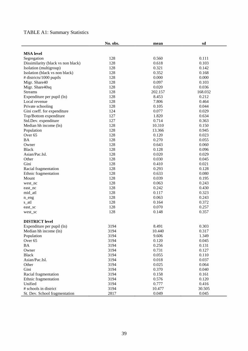
mental variables, we constructed shares of minority immigrants using datafrom the Census of Population and Housing, Public Use Microdata Sample1940 (PUMS 1940).13 The streams variables are extracted from the datasetused by Rothstein (2005).14 Summary statistics of all variables employed arecontained in Appendix table A1.

5.1 Racial segregation and fragmentation

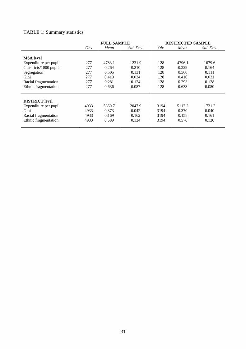
Table 1 contains descriptive statistics for some variables of interest at theMSA level. In all our empirical analysis we restrict attention to metropolitanareas whose minority population is at least 5% of the total. This is becausethe meaningfulness of the segregation indexes is very limited otherwise. Ourworking sample consists of 277 MSAs for the OLS regressions and is restrictedto 128 MSAs when we instrument segregation with the share of minority im-migrants in 1940. This reduction in sample size is due to the smaller numberof Statistical Metropolitan Areas in 1940. In the district level regressions(for which we only report the restricted sample results), we have a total of3,194 school districts in the 128 metropolitan areas.

[Insert Tables 1 and 2]

Expenditure per student in the average MSA is 4,783 US dollars (in 1990prices), with a standard deviation of 1,232 dollars; average figures for therestricted sample are virtually identical. The high variability in expenditureper student is more apparent if we look at district level data, where the corre-sponding figures are, respectively, 5,361 and 2,048 dollars for the full sampleand 5,112 and 1,721 dollars for the restricted one. The number of districtsalso varies a lot across metropolitan areas. The average MSA has .26 dis-tricts for every 1,000 students (.23 in the restricted sample), but the rangeof this variable goes from .003 to 1.11 districts per 1,000 students. Turningto heterogeneity in income, race and ethnic origin, we see that individualdistricts are less heterogeneous than metropolitan areas: the average Ginicoefficient on household income is .41 for the MSA and .37 for the district;racial fragmentation is on average .28 in the MSA and only .17 in the dis-trict, and similarly for ethnic fragmentation. As for segregation, in order to13The PUMS 1940 is a 1% stratified sample of households extracted from Census of

Population and Housing. We used the data provided by ICPSR, from ICPSR Study No.8236.14We used the data available online at http://www.princeton.edu/~jrothst/replication/hoxbydocumentation/fi

16

achieve an even distribution on the territory in the average MSA, 51% ofthe population should move from one Census tract to another (56% in therestricted sample). Note that the measures of income inequality, racial andethnic fragmentation are almost identical across samples (full and restricted).

[Insert Figures 2-4]

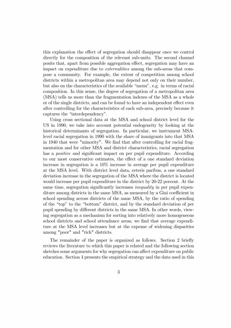
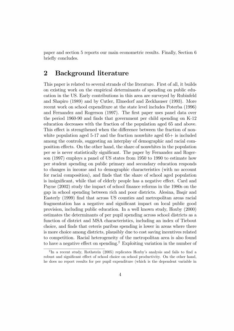
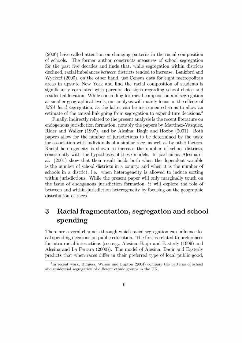
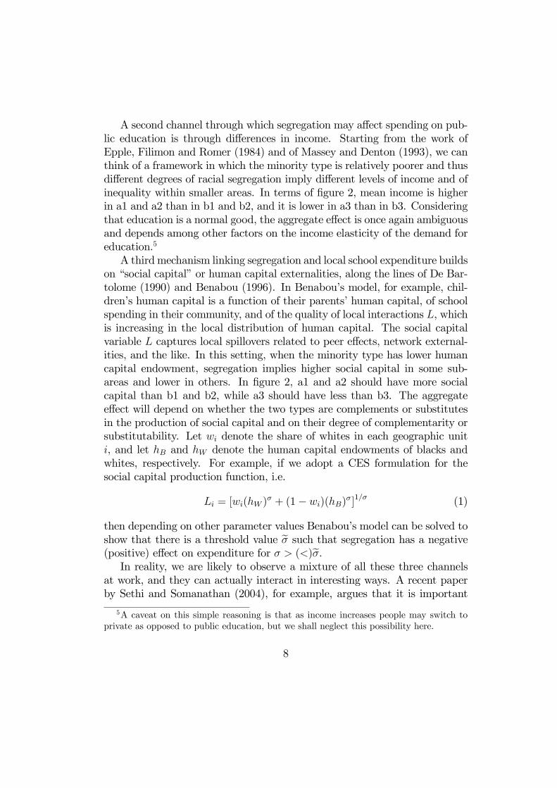
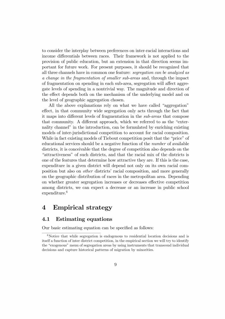
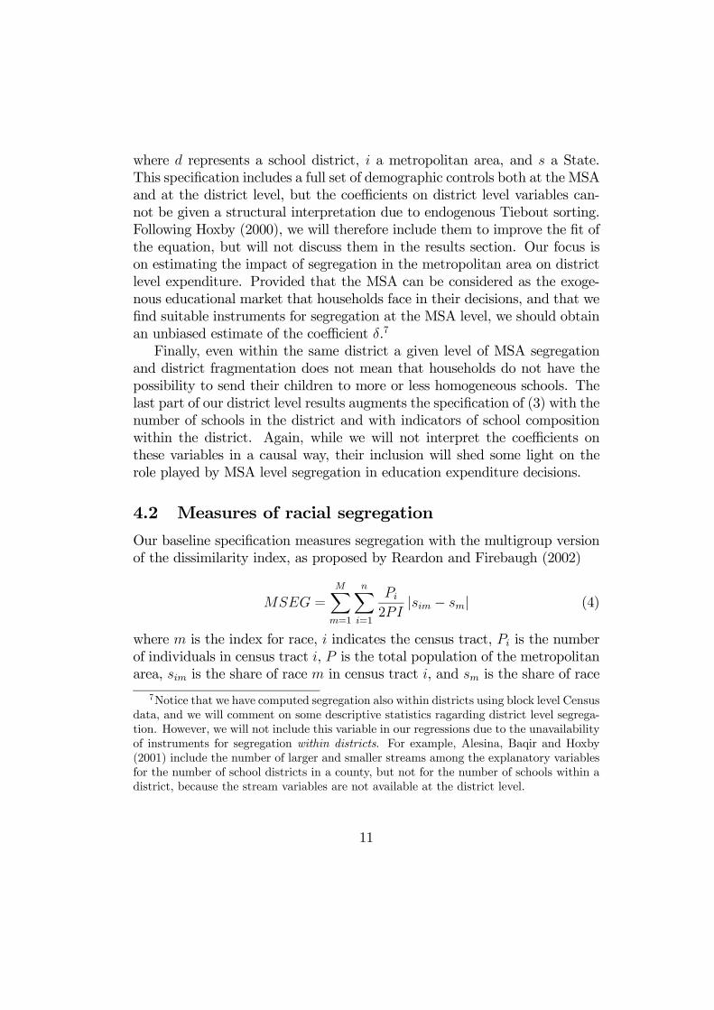
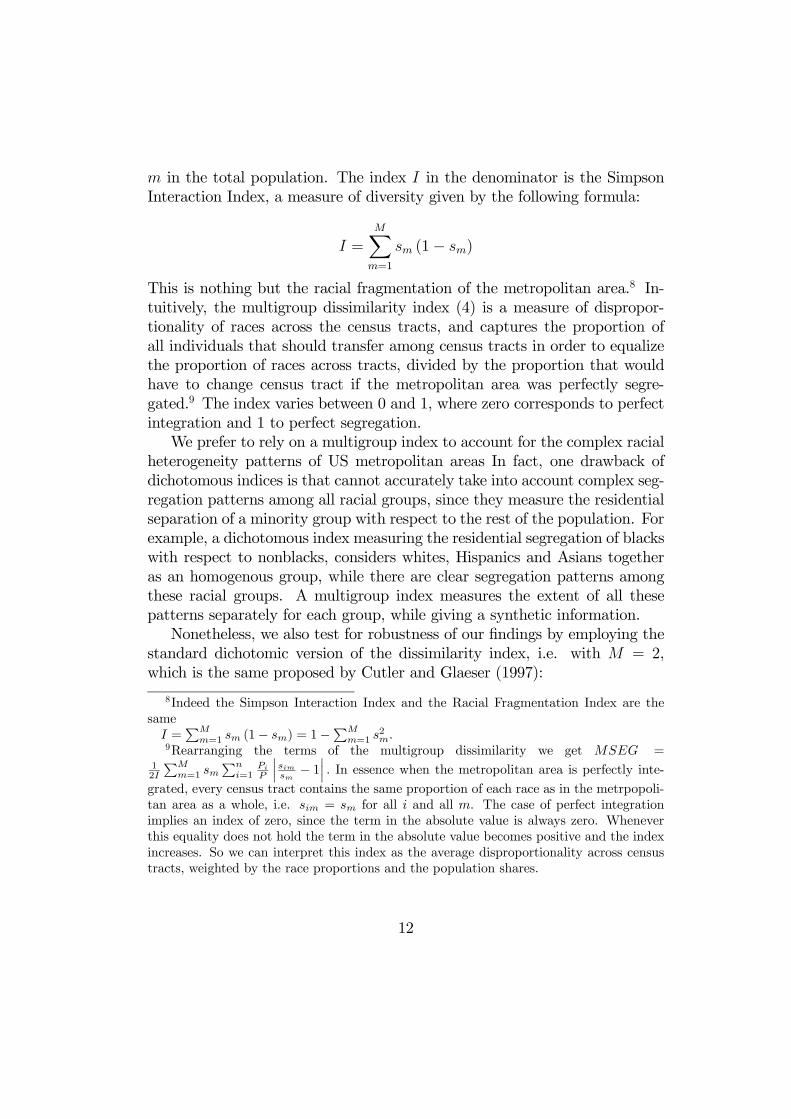
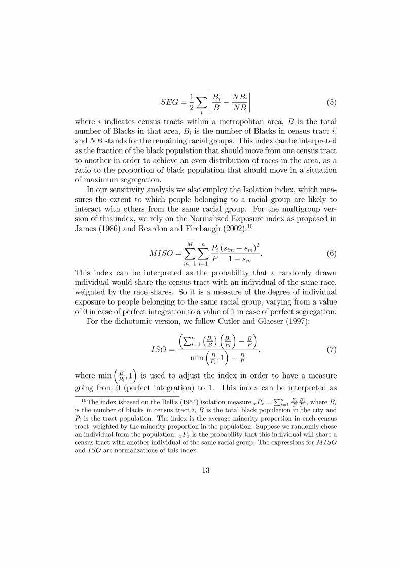
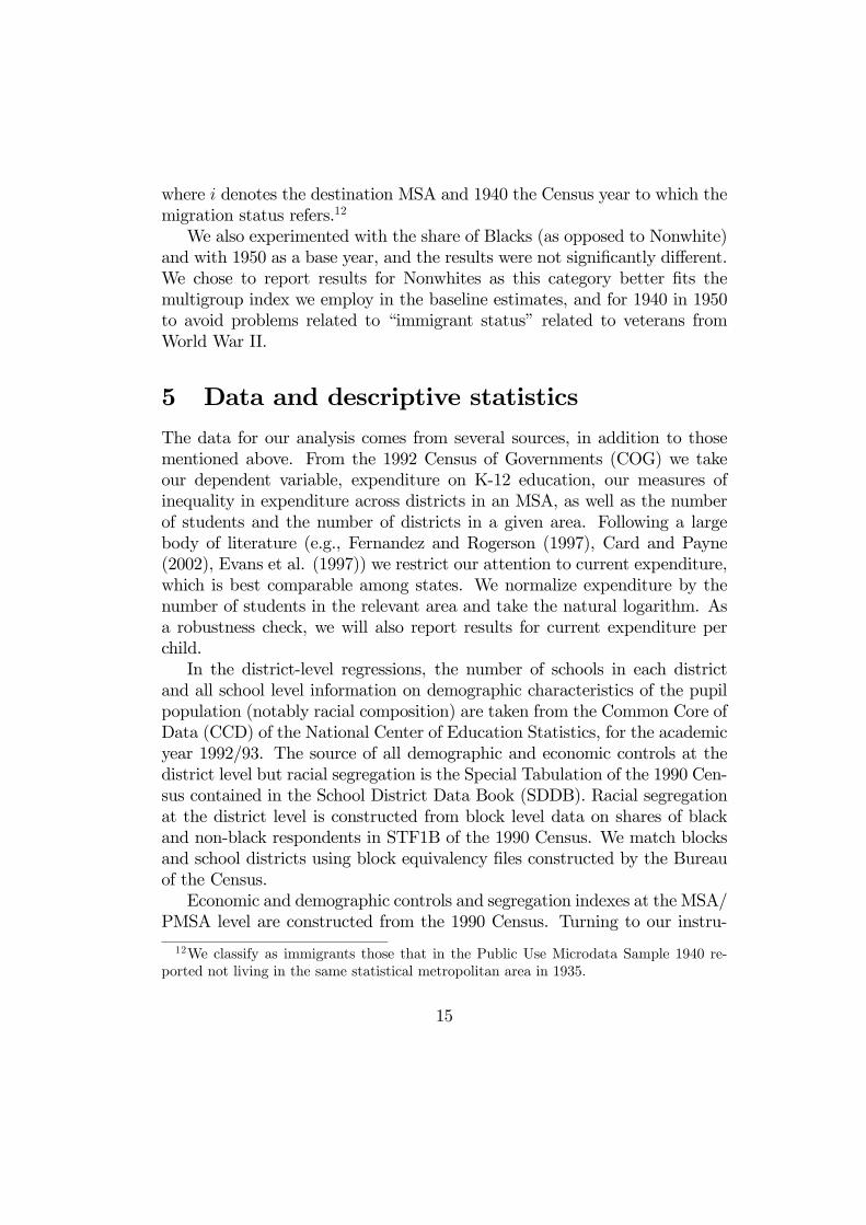
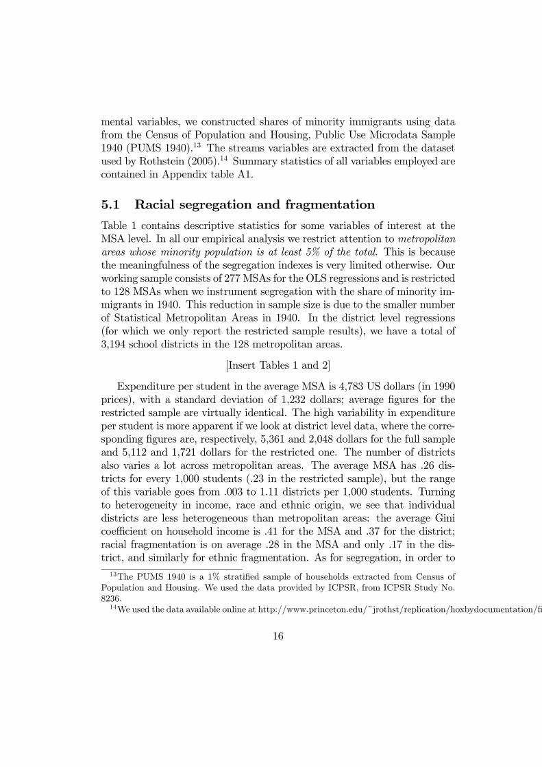
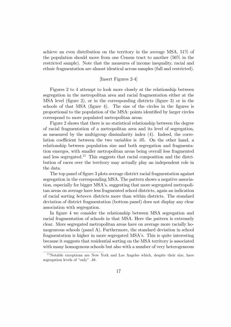
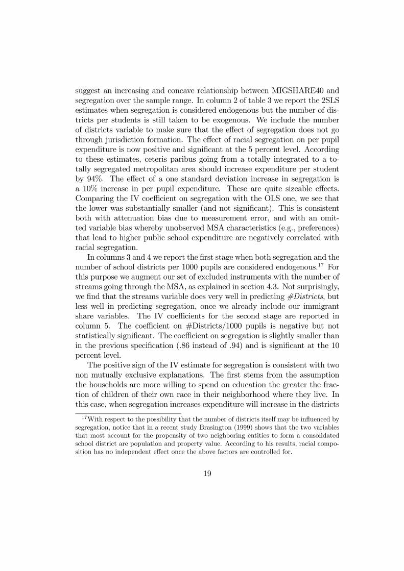
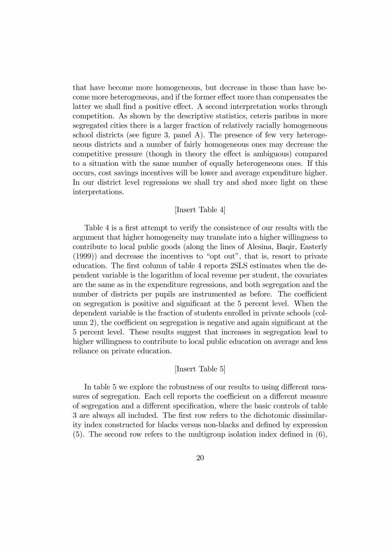
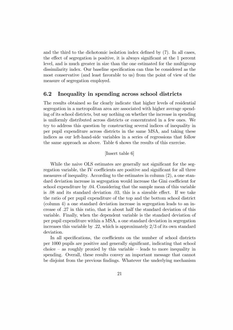
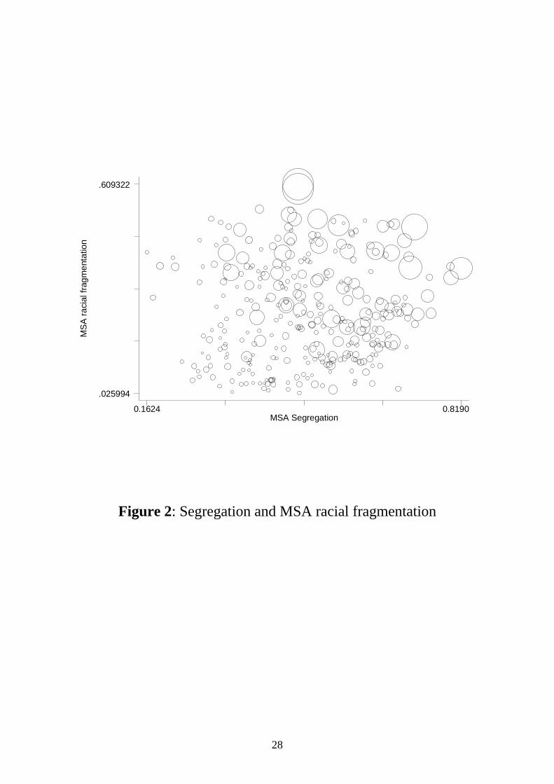
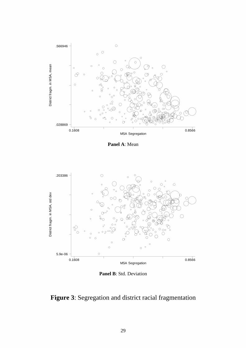
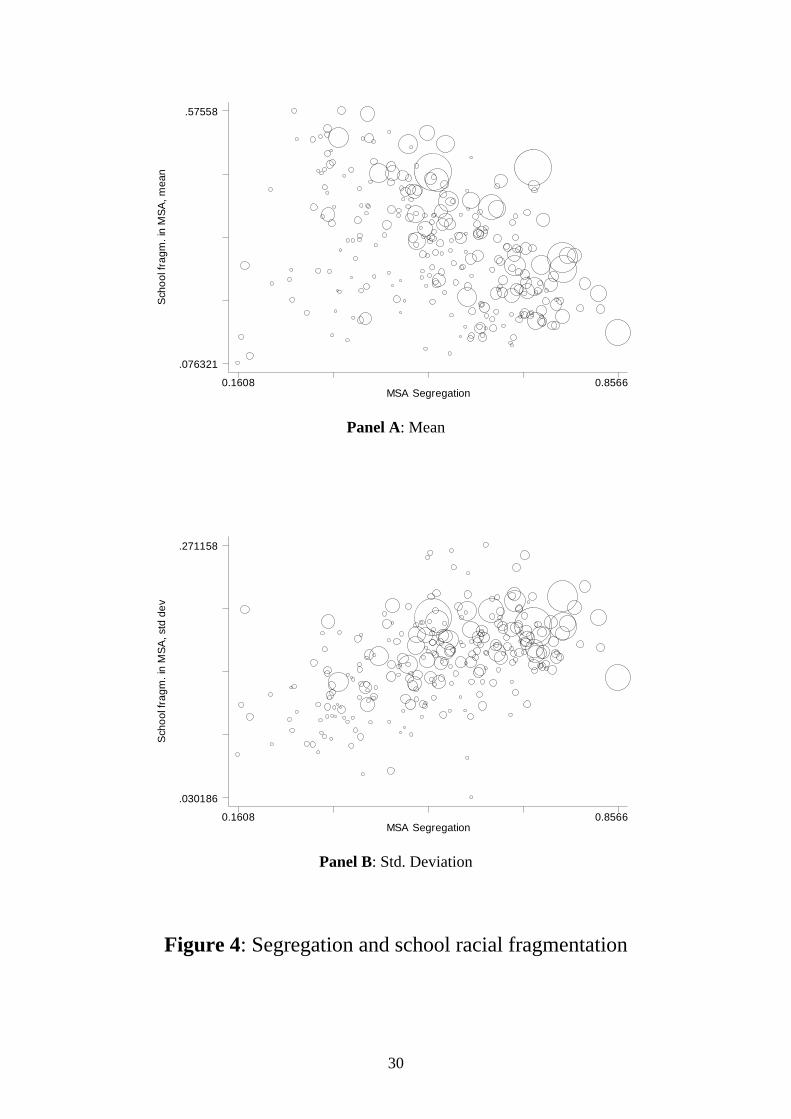
Figures 2 to 4 attempt to look more closely at the relationship betweensegregation in the metropolitan area and racial fragmentation either at theMSA level (figure 2), or in the corresponding districts (figure 3) or in theschools of that MSA (figure 4). The size of the circles in the figures isproportional to the population of the MSA: points identified by larger circlescorrespond to more populated metropolitan areas.Figure 2 shows that there is no statistical relationship between the degree

of racial fragmentation of a metropolitan area and its level of segregation,as measured by the multigroup dissimilarity index (4). Indeed, the corre-lation coefficient between the two variables is .05. On the other hand, arelationship between population size and both segregation and fragmenta-tion emerges, with smaller metropolitan areas being overall less fragmentedand less segregated.15 This suggests that racial composition and the distri-bution of races over the territory may actually play an independent role inthe data.The top panel of figure 3 plots average district racial fragmentation against

segregation in the corresponding MSA. The pattern shows a negative associa-tion, especially for bigger MSA’s, suggesting that more segregated metropoli-tan areas on average have less fragmented school districts, again an indicationof racial sorting between districts more than within districts. The standarddeviation of district fragmentation (bottom panel) does not display any clearassociation with segregation.In figure 4 we consider the relationship between MSA segregation and

racial fragmentation of schools in that MSA. Here the pattern is extremelyclear. More segregated metropolitan areas have on average more racially ho-mogeneous schools (panel A). Furthermore, the standard deviation in schoolfragmentation is higher in more segregated MSA’s. This is quite interestingbecause it suggests that residential sorting on the MSA territory is associatedwith many homogenous schools but also with a number of very heterogeneous

15Notable exceptions are New York and Los Angeles which, despite their size, havesegregation levels of “only” .48.

17

ones. As briefly sketched in the theoretical section, this pattern is likely togenerate different desired expenditure levels by households than a patternwith the same average school heterogeneity but no variation among schools.We next move to multivariate analysis.

6 Empirical results

6.1 Average school spending, MSA level

[Insert Table 2]

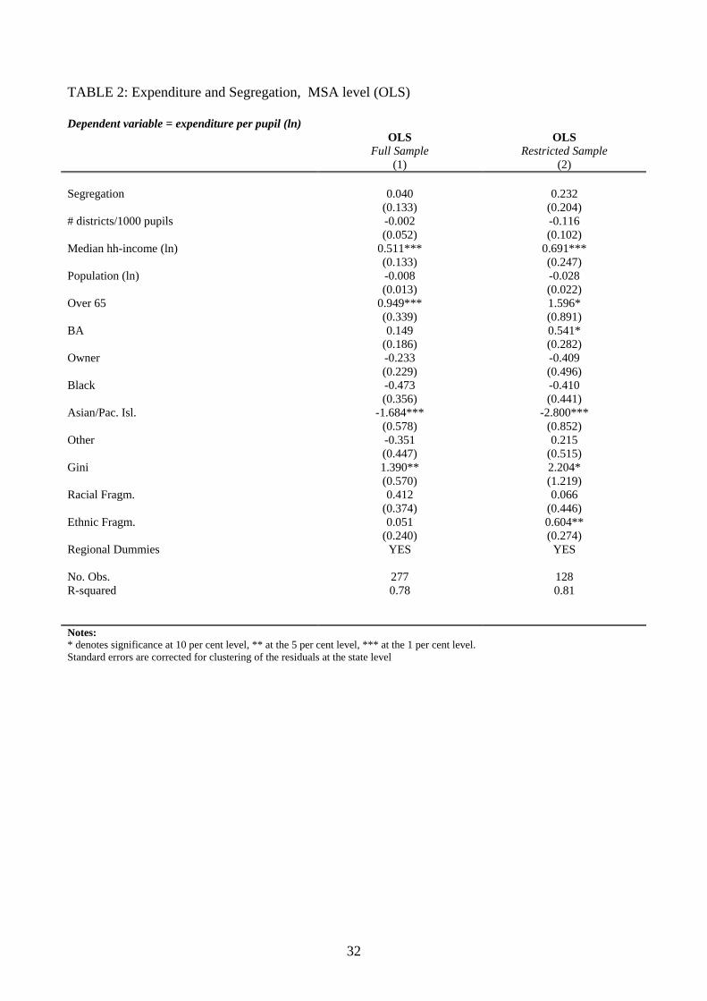
Table 2 presents naive OLS estimates of the determinants of expenditureper student at the MSA level. Column 1 reports estimates for the full sample,and column 2 for the restricted sample (that is, the subset of metropolitanareas for which we have migration data by race in 1940). Included regres-sors are the multigroup dissimilarity index (from now on, “Segregation”),the number of school districts per 1000 pupils, median household income (inlogs), the population (in logs), the share of the population aged 65 or more,the share with education level BA or higher, the fraction of home owners,the share of African American, Asians/Pacific islanders, and other races (theomitted category is white), the Gini coefficient of inequality in household to-tal taxable income, racial fragmentation and ethnic fragmentation as definedin Alesina and La Ferrara (2000). All regressions include the nine Censusregion dummies. The most notable difference with respect to previous stud-ies is that we do not find a negative coefficient on the racial fragmentationvariable, possibly due to the exclusion from our sample of MSA’s with lessthan 5% of minority population. The coefficient on racial segregation is notsignificant, nor is that on the school district variable, regardless of the sampleconsidered.16

[Insert Table 3]

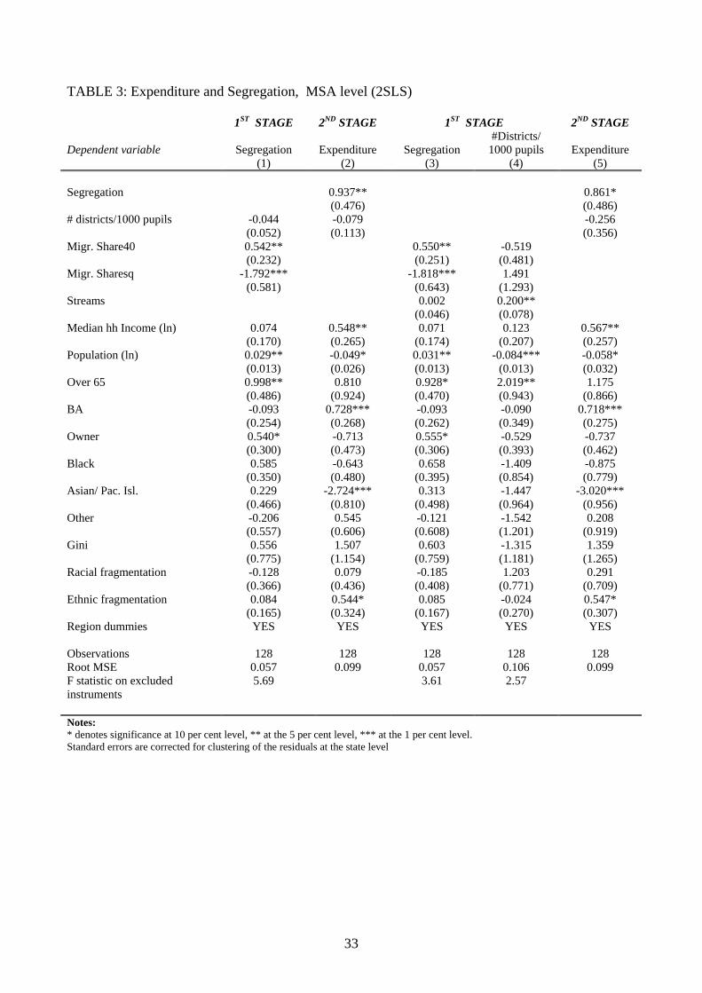
Table 3 contains our main empirical results. In column 1 we report ourfirst stage regression, where the excluded instruments are the share of mi-nority immigrants in 1940 (as defined in expression (8)) and its square. Thisvariables turn out to be highly significant, and the estimated coefficients

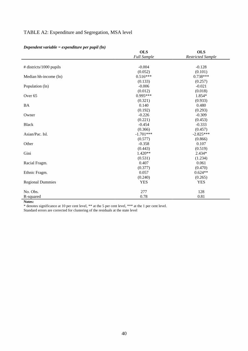
16Appendix table A2 reports estimates on other covariates when segregation is notincluded among the regressors.

18

suggest an increasing and concave relationship between MIGSHARE40 andsegregation over the sample range. In column 2 of table 3 we report the 2SLSestimates when segregation is considered endogenous but the number of dis-tricts per students is still taken to be exogenous. We include the numberof districts variable to make sure that the effect of segregation does not gothrough jurisdiction formation. The effect of racial segregation on per pupilexpenditure is now positive and significant at the 5 percent level. Accordingto these estimates, ceteris paribus going from a totally integrated to a to-tally segregated metropolitan area should increase expenditure per studentby 94%. The effect of a one standard deviation increase in segregation isa 10% increase in per pupil expenditure. These are quite sizeable effects.Comparing the IV coefficient on segregation with the OLS one, we see thatthe lower was substantially smaller (and not significant). This is consistentboth with attenuation bias due to measurement error, and with an omit-ted variable bias whereby unobserved MSA characteristics (e.g., preferences)that lead to higher public school expenditure are negatively correlated withracial segregation.In columns 3 and 4 we report the first stage when both segregation and the

number of school districts per 1000 pupils are considered endogenous.17 Forthis purpose we augment our set of excluded instruments with the number ofstreams going through the MSA, as explained in section 4.3. Not surprisingly,we find that the streams variable does very well in predicting #Districts, butless well in predicting segregation, once we already include our immigrantshare variables. The IV coefficients for the second stage are reported incolumn 5. The coefficient on #Districts/1000 pupils is negative but notstatistically significant. The coefficient on segregation is slightly smaller thanin the previous specification (.86 instead of .94) and is significant at the 10percent level.The positive sign of the IV estimate for segregation is consistent with two

non mutually exclusive explanations. The first stems from the assumptionthe households are more willing to spend on education the greater the frac-tion of children of their own race in their neighborhood where they live. Inthis case, when segregation increases expenditure will increase in the districts

17With respect to the possibility that the number of districts itself may be influenced bysegregation, notice that in a recent study Brasington (1999) shows that the two variablesthat most account for the propensity of two neighboring entities to form a consolidatedschool district are population and property value. According to his results, racial compo-sition has no independent effect once the above factors are controlled for.

19

that have become more homogeneous, but decrease in those than have be-come more heterogeneous, and if the former effect more than compensates thelatter we shall find a positive effect. A second interpretation works throughcompetition. As shown by the descriptive statistics, ceteris paribus in moresegregated cities there is a larger fraction of relatively racially homogeneousschool districts (see figure 3, panel A). The presence of few very heteroge-neous districts and a number of fairly homogeneous ones may decrease thecompetitive pressure (though in theory the effect is ambiguous) comparedto a situation with the same number of equally heterogeneous ones. If thisoccurs, cost savings incentives will be lower and average expenditure higher.In our district level regressions we shall try and shed more light on theseinterpretations.

[Insert Table 4]

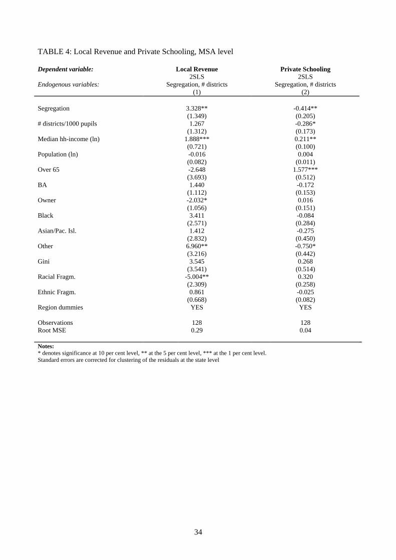
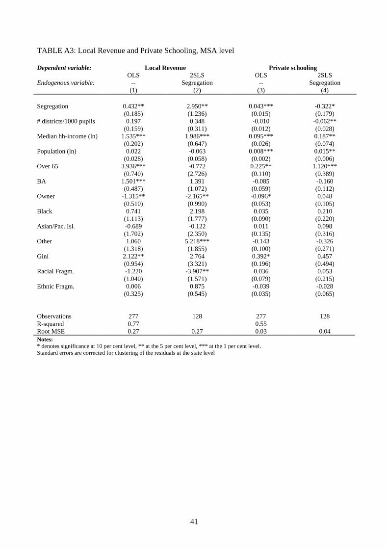
Table 4 is a first attempt to verify the consistence of our results with theargument that higher homogeneity may translate into a higher willingness tocontribute to local public goods (along the lines of Alesina, Baqir, Easterly(1999)) and decrease the incentives to “opt out”, that is, resort to privateeducation. The first column of table 4 reports 2SLS estimates when the de-pendent variable is the logarithm of local revenue per student, the covariatesare the same as in the expenditure regressions, and both segregation and thenumber of districts per pupils are instrumented as before. The coefficienton segregation is positive and significant at the 5 percent level. When thedependent variable is the fraction of students enrolled in private schools (col-umn 2), the coefficient on segregation is negative and again significant at the5 percent level. These results suggest that increases in segregation lead tohigher willingness to contribute to local public education on average and lessreliance on private education.

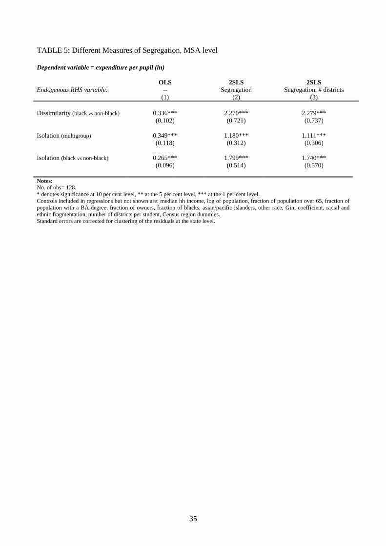
[Insert Table 5]

In table 5 we explore the robustness of our results to using different mea-sures of segregation. Each cell reports the coefficient on a different measureof segregation and a different specification, where the basic controls of table3 are always all included. The first row refers to the dichotomic dissimilar-ity index constructed for blacks versus non-blacks and defined by expression(5). The second row refers to the multigroup isolation index defined in (6),

20

and the third to the dichotomic isolation index defined by (7). In all cases,the effect of segregation is positive, it is always significant at the 1 percentlevel, and is much greater in size than the one estimated for the multigroupdissimilarity index. Our baseline specification can thus be considered as themost conservative (and least favorable to us) from the point of view of themeasure of segregation employed.

6.2 Inequality in spending across school districts

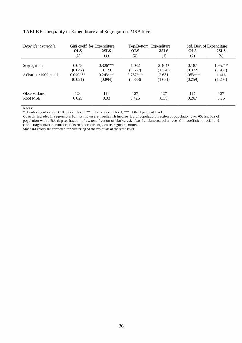
The results obtained so far clearly indicate that higher levels of residentialsegregation in a metropolitan area are associated with higher average spend-ing of its school districts, but say nothing on whether the increase in spendingis uniformly distributed across districts or concentrated in a few ones. Wetry to address this question by constructing several indices of inequality inper pupil expenditure across districts in the same MSA, and taking theseindices as our left-hand-side variables in a series of regressions that followthe same approach as above. Table 6 shows the results of this exercise.

[Insert table 6]

While the naive OLS estimates are generally not significant for the seg-regation variable, the IV coefficients are positive and significant for all threemeasures of inequality. According to the estimates in column (2), a one stan-dard deviation increase in segregation would increase the Gini coefficient forschool expenditure by .04. Considering that the sample mean of this variableis .08 and its standard deviation .03, this is a sizeable effect. If we takethe ratio of per pupil expenditure of the top and the bottom school district(column 4) a one standard deviation increase in segregation leads to an in-crease of .27 in this ratio, that is about half the standard deviation of thisvariable. Finally, when the dependent variable is the standard deviation ofper pupil expenditure within a MSA, a one standard deviation in segregationincreases this variable by .22, which is approximately 2/3 of its own standarddeviation.In all specifications, the coefficients on the number of school districts

per 1000 pupils are positive and generally significant, indicating that schoolchoice — as roughly proxied by this variable — leads to more inequality inspending. Overall, these results convey an important message that cannotbe disjoint from the previous findings. Whatever the underlying mechanism

21

why residential segregation translates into more resources devoted to publiceducation in the aggregate, it does so at the expense of the low spendingdistricts that see a widening gap in per pupil spending compared to richerdistricts.

6.3 Evidence at the district level

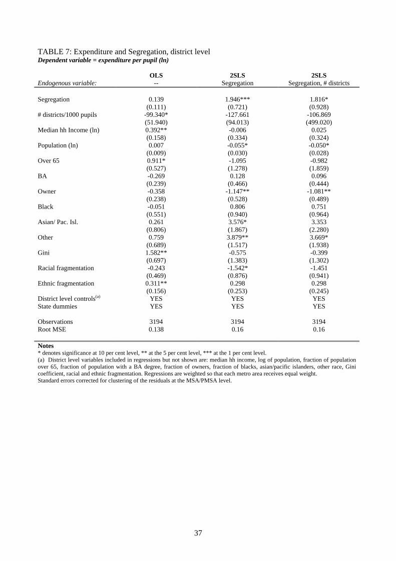
In this section we analyze the determinants of expenditure at the districtlevel, including both a district’s own characteristics (demographics, incomedistribution, racial composition) and the characteristics of the MSA wherethe district is located. Only the coefficients on the MSA variables are in-terpretable and are therefore reported. The list of district level controls(reported in the tables) is anyway the same as that of city level controls,except for the addition of a dummy for unified school districts, to controlfor the fact that unified districts have greater outlays. State fixed effects areincluded to control for differences in school financing policies across States.All observations are weighted so that every MSA has the same probabilityof being in the sample.

[Insert table 7]

Table 7 reports three sets of estimates: naive OLS, 2SLS with one en-dogenous variable (segregation), and 2SLS with two endogenous regressors(segregation and#Districts). The pattern on the segregation variable mimicsthat of the MSA level regressions. Our estimate in columns 2 and 3 suggeststhat, ceteris paribus, “moving a district” from a totally integrated to a totallysegregated MSA would almost double per pupil expenditure in that district.Ceteris paribus, a one standard deviation increase in the segregation of theMSA where the district is located would increase per pupil expenditure inthe district by 22 percent (column 2) or 20 percent (column 3). Notice thatthis holds after controlling for the racial fragmentation of the district itself.Given that the ‘demand’ effect that associates changes in segregation withchanges in district level fragmentation should be picked up by the own dis-trict fragmentation variable, the positive coefficient on segregation is likelyto reflect externalities among districts.

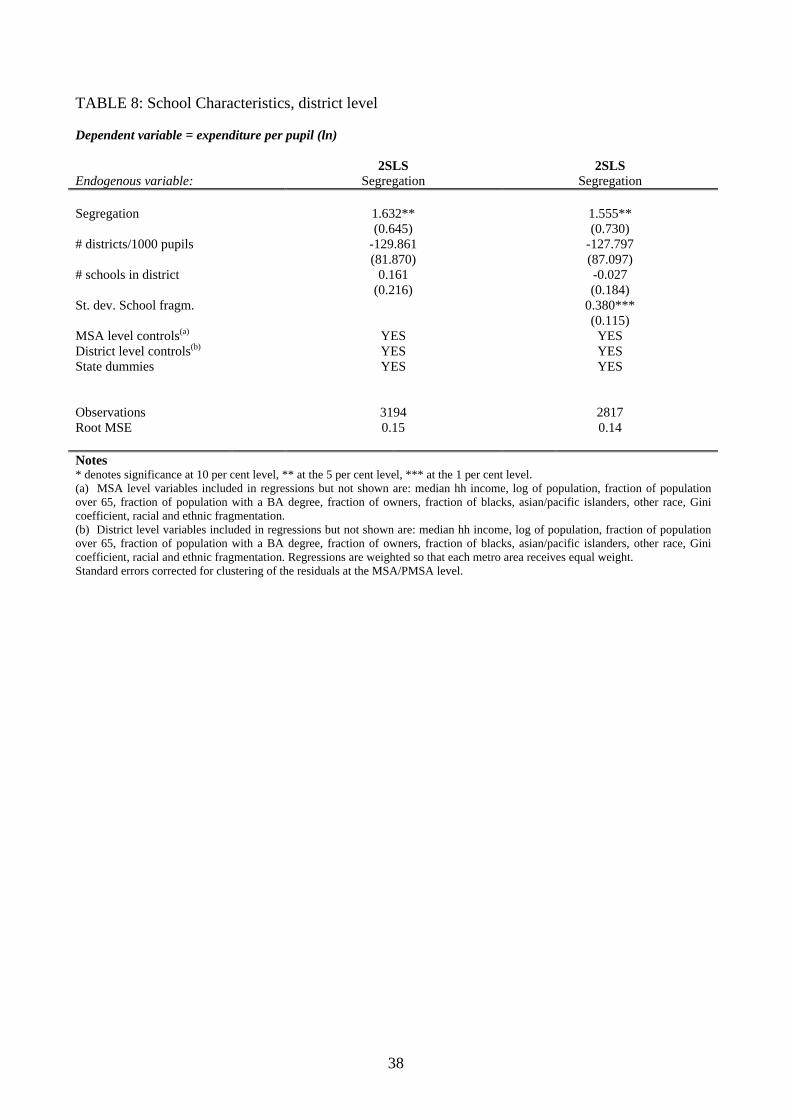
[Insert table 8]

22

In table 8 we include two variables that are meant to proxy for the menuof choices among schools available to parents. The idea is that, if inter-racialcontact in the school is what matters, the availability of a large number ofschools and the variation in the degree of school heterogeneity may play animportant role. The first column of table 8 includes, in addition to the usualcontrols, the number of schools in the district. This variable is not signifi-cant, while segregation retains a positive and significant effect on spending.In the second column we also add the standard deviation of school levelracial fragmentation. The latter variable is particularly relevant in that itcaptures the degree of variation in the heterogeneity of the pupils population.In fact, what matters is not the mean level of fragmentation but its disper-sion, because it accounts for whether a metropolitan area contains schoolswhose racial composition is broadly similar or very diverse. The coefficienton this variable is positive and significant, and even in this specification thecoefficient on segregation remains stable and significant.

7 Conclusions

This paper has addressed the question of whether racial segregation affectsspending on public education, and has provided suggestive evidence thatsegregation has a positive impact on average per pupil expenditure, bothat the metropolitan area and at the district level. However, our estimatesalso show that increased segregation leads to more inequality in spendingacross districts of the same MSA. Although further work is needed to pindown the mechanisms through which segregation impacts on public educa-tion provision, the results in this paper point to yet one more undesirable eco-nomic effect of racial segregation. In addition to directly worsening economicoutcomes of minority groups, as known in the literature, increased segrega-tion seems to cause lower investments in public education by poorer schooldistricts relative to richer ones, which further undermines the prospects ofupward mobility for disadvantaged people.

References

[1] Alesina, A., R. Baqir andW. Easterly (1999), “Public Goods and EthnicDivisions”, Quarterly Journal of Economics, 114(4), 1243-1284.

23

[2] Alesina, A., R. Baqir and C. Hoxby (2000), “Political Jurisdictions inHeterogeneous Communities”, NBER Working Paper 7859.

[3] Alesina, A. and E. La Ferrara (2000), “Participation in HeterogeneousCommunities”, Quarterly Journal of Economics, 115, 847-904.

[4] Benabou, R. (1996), “Equity and Efficiency in Human Capital Invest-ment: The Local Connection”, Review of Economic Studies, 63, 237-264.

[5] Borjas, G. (1995), “Ethnicity, Neighborhood and Human Capital Exter-nalities”, American Economic Review, 85, 365-390.

[6] Brasington, D.M. (1999), “Joint Provision of Public Goods: The Consol-idation of School Districts”, Journal of Public Economics, 73, 373-393.

[7] Burgess, S., D. Wilson and R. Lupton (2004), “Parallel Lives? EthnicSegregation in the Playground and the Neighborhood”, mimeo, Univer-sity of Bristol.

[8] Card, D. and A. Payne (2002), “Schoold Finance Reform, the Distribu-tion of School Spending, and the Distribution of Student Test Scores”,Journal of Public Economics, 83(1), pp.49-82.

[9] Card, D. and J. Rothstein (2005), “Racial Segregation and the Black-White Test Score Gap”, mimeo, UC Berkeley and Princeton University.

[10] Case, A. and L. Katz (1991), “The Company You Keep: The Effect ofFamily and Neighborhood on Disadvantaged Youth”, NBER WorkingPaper 3705.

[11] Clotfelter, C. (2004), After Brown: The Rise and Retreat of School De-segregation, Princeton: Princeton University Press.

[12] Collins, W. (1997), “When the Tide Turned: Immigration and the Delayof the Great Black Migration”, Journal of Economic History, 57(3), 607-632.

[13] Cutler, D., D. Elmendorf and R. Zeckhauser (1993), “DemographicCharacteristics and the Public Bundle”, Public Finance, 48, 178-198.

[14] Cutler, D. and E. Glaeser (1997), “Are Ghettos Good or Bad?”, Quar-terly Journal of Economics, 112(3), 827-872.

24

[15] De Bartolome, C. (1990), “Equilibrium and Inefficiency in a CommunityModel with Peer Group Effects”, Journal of Political Economy, 98(19,110-133.

[16] Epple, D. R. Filimon and T. Romer (1984), “Equilibrium Among LocalJurisdictions: Toward an Integrated Traetment of Voting and Residen-tial Choice”, Journal of Public Economics, 24, 281-308.

[17] Evans, W., S. Murray and R. Schwab (1997), “Schoolhouses, Court-houses and Statehouses after Serrano”, Journal of Policy Analysis andManagement, 16(1), 10-31.

[18] Fernandez, R. and R. Rogerson (1996),“Income Distribution, Commu-nities, and the Quality of Public Education”, Quarterly Journal of Eco-nomics, February, 135-164.

[19] ____ (1997), “The Determinants of Public Education Expenditures:Evidence from the States”, NBER Working Paper 5995.

[20] Guryan, J. (2004), “Desegregation and Black Dropout Rates”, AmericanEconomic Review, 94(4), 919-43.

[21] Hoxby, C. (2000), “Does Competition among Public Schools Benefit Stu-dents and Taxpayers?”, American Economic Review, December, 1209-1238.

[22] Kain, J. (1968), “The Spatial Mismatch Hypothesis: Three DecadesTogether”, Housing Policy Debate, 3, 371-462.

[23] James, Franklyn J. (1986), "A New Generalized "Exposure-Based" Seg-regation Index", Sociological Methods and Research, 14, 301-316

[24] Lankford, H. and J. Wyckoff (2000), “The Effect of School Choice andResidential Location on the Racial Segregation of Students”, mimeo,SUNY Albany.

[25] Margo, R. (1998), “Schooling and the Great Migration”, NBERWorkingPaper 2697.

[26] Martinez-Vazquez, J., M. Rider and M.B. Walker (1997), “Race and theStructure of School Districts in the United States”, Journal of UrbanEconomics, 41, 281-300.

25

[27] Poterba, J. (1996), “Demographic Structure and the Political Economyof Public Education”, NBER Working Paper 5677.

[28] Reardon, Sean F. and Glenn Firebaugh (2002), "Measures of MultigroupSegregation", Sociological Methodology, 32, 33-67

[29] Ross, S.L. (2001), “Segregation and Racial Preferences: An Analysis ofChoice Based on Satisfaction and Outcome Measures”, mimeo, Univer-sity of Connecticut.

[30] Rothstein, J. (2005), “Does Competition among Public Schools BenefitStudents and Taxpayers? A Comment on Hoxby (2000)”, AmericanEconomic Review, forthcoming.

[31] Rubinfeld, D. and P. Shapiro (1989), “Micro-estimation of the Demandfor Schooling: Evidence from Michigan and Massachusetts”, RegionalScience and Urban Economics, 19, 381-398.

[32] Sethi, Rajiv and Rohini Somanathan (2004), “Inequality and Segrega-tion”, Journal of Political Economy, 112(6), 1296-1322.

[33] Urquiola, M. (1999), “Demand Matters: School District Concentration,Composition, and Educational Expenditure”, mimeo, UC Berkeley.

[34] Wilson, W. (1987), The Truly Disadvantaged: The Inner City, the Un-derclass, and Public Policy, Chicago: University of Chicago Press.

26

27

a1 a2 a3 b1 b2 b3

Figure 1: Racial fragmentation vs. segregation

A: Perfect Segregation B: Perfect Integration

28

MS

A ra

cial

frag

men

tatio

n

MSA Segregation0.1624 0.8190

.025994

.609322

Figure 2: Segregation and MSA racial fragmentation

29

Dist

rict f

ragm

. in

MSA

, mea

n

MSA Segregation0.1608 0.8566

.028869

.566946

Panel A: Mean

Dist

rict f

ragm

. in

MSA

, std

dev

MSA Segregation0.1608 0.8566

5.9e-06

.203386

Panel B: Std. Deviation

Figure 3: Segregation and district racial fragmentation

30

Sch

ool f

ragm

. in

MSA

, mea

n

MSA Segregation0.1608 0.8566

.076321

.57558

Panel A: Mean

Sch

ool f

ragm

. in

MSA

, std

dev

MSA Segregation0.1608 0.8566

.030186

.271158

Panel B: Std. Deviation

Figure 4: Segregation and school racial fragmentation

31

TABLE 1: Summary statistics FULL SAMPLE RESTRICTED SAMPLE Obs Mean Std. Dev. Obs Mean Std. Dev. MSA level

Expenditure per pupil 277 4783.1 1231.9 128 4796.1 1079.6 # districts/1000 pupils 277 0.264 0.210 128 0.229 0.164 Segregation 277 0.505 0.131 128 0.560 0.111 Gini 277 0.410 0.024 128 0.410 0.021 Racial fragmentation 277 0.281 0.124 128 0.293 0.128 Ethnic fragmentation 277 0.636 0.087 128 0.633 0.080 DISTRICT level Expenditure per pupil 4933 5360.7 2047.9 3194 5112.2 1721.2 Gini 4933 0.373 0.042 3194 0.370 0.040 Racial fragmentation 4933 0.169 0.162 3194 0.158 0.161 Ethnic fragmentation 4933 0.589 0.124 3194 0.576 0.120

32

TABLE 2: Expenditure and Segregation, MSA level (OLS) Dependent variable = expenditure per pupil (ln) OLS OLS Full Sample Restricted Sample (1) (2) Segregation 0.040 0.232 (0.133) (0.204) # districts/1000 pupils -0.002 -0.116 (0.052) (0.102) Median hh-income (ln) 0.511*** 0.691*** (0.133) (0.247) Population (ln) -0.008 -0.028 (0.013) (0.022) Over 65 0.949*** 1.596* (0.339) (0.891) BA 0.149 0.541* (0.186) (0.282) Owner -0.233 -0.409 (0.229) (0.496) Black -0.473 -0.410 (0.356) (0.441) Asian/Pac. Isl. -1.684*** -2.800*** (0.578) (0.852) Other -0.351 0.215 (0.447) (0.515) Gini 1.390** 2.204* (0.570) (1.219) Racial Fragm. 0.412 0.066 (0.374) (0.446) Ethnic Fragm. 0.051 0.604** (0.240) (0.274) Regional Dummies YES YES No. Obs. 277 128 R-squared 0.78 0.81 Notes: * denotes significance at 10 per cent level, ** at the 5 per cent level, *** at the 1 per cent level. Standard errors are corrected for clustering of the residuals at the state level

33

TABLE 3: Expenditure and Segregation, MSA level (2SLS) 1ST STAGE 2ND STAGE 1ST STAGE 2ND STAGE Dependent variable

Segregation

Expenditure

Segregation

#Districts/ 1000 pupils

Expenditure

(1) (2) (3) (4) (5) Segregation 0.937** 0.861* (0.476) (0.486) # districts/1000 pupils -0.044 -0.079 -0.256 (0.052) (0.113) (0.356) Migr. Share40 0.542** 0.550** -0.519 (0.232) (0.251) (0.481) Migr. Sharesq -1.792*** -1.818*** 1.491 (0.581) (0.643) (1.293) Streams 0.002 0.200** (0.046) (0.078) Median hh Income (ln) 0.074 0.548** 0.071 0.123 0.567** (0.170) (0.265) (0.174) (0.207) (0.257) Population (ln) 0.029** -0.049* 0.031** -0.084*** -0.058* (0.013) (0.026) (0.013) (0.013) (0.032) Over 65 0.998** 0.810 0.928* 2.019** 1.175 (0.486) (0.924) (0.470) (0.943) (0.866) BA -0.093 0.728*** -0.093 -0.090 0.718*** (0.254) (0.268) (0.262) (0.349) (0.275) Owner 0.540* -0.713 0.555* -0.529 -0.737 (0.300) (0.473) (0.306) (0.393) (0.462) Black 0.585 -0.643 0.658 -1.409 -0.875 (0.350) (0.480) (0.395) (0.854) (0.779) Asian/ Pac. Isl. 0.229 -2.724*** 0.313 -1.447 -3.020*** (0.466) (0.810) (0.498) (0.964) (0.956) Other -0.206 0.545 -0.121 -1.542 0.208 (0.557) (0.606) (0.608) (1.201) (0.919) Gini 0.556 1.507 0.603 -1.315 1.359 (0.775) (1.154) (0.759) (1.181) (1.265) Racial fragmentation -0.128 0.079 -0.185 1.203 0.291 (0.366) (0.436) (0.408) (0.771) (0.709) Ethnic fragmentation 0.084 0.544* 0.085 -0.024 0.547* (0.165) (0.324) (0.167) (0.270) (0.307) Region dummies YES YES YES YES YES Observations 128 128 128 128 128 Root MSE 0.057 0.099 0.057 0.106 0.099 F statistic on excluded instruments

5.69 3.61 2.57

Notes: * denotes significance at 10 per cent level, ** at the 5 per cent level, *** at the 1 per cent level. Standard errors are corrected for clustering of the residuals at the state level

34

TABLE 4: Local Revenue and Private Schooling, MSA level Dependent variable: Local Revenue Private Schooling 2SLS 2SLS Endogenous variables: Segregation, # districts Segregation, # districts (1) (2) Segregation 3.328** -0.414** (1.349) (0.205) # districts/1000 pupils 1.267 -0.286* (1.312) (0.173) Median hh-income (ln) 1.888*** 0.211** (0.721) (0.100) Population (ln) -0.016 0.004 (0.082) (0.011) Over 65 -2.648 1.577*** (3.693) (0.512) BA 1.440 -0.172 (1.112) (0.153) Owner -2.032* 0.016 (1.056) (0.151) Black 3.411 -0.084 (2.571) (0.284) Asian/Pac. Isl. 1.412 -0.275 (2.832) (0.450) Other 6.960** -0.750* (3.216) (0.442) Gini 3.545 0.268 (3.541) (0.514) Racial Fragm. -5.004** 0.320 (2.309) (0.258) Ethnic Fragm. 0.861 -0.025 (0.668) (0.082) Region dummies YES YES Observations 128 128 Root MSE

0.29 0.04

Notes: * denotes significance at 10 per cent level, ** at the 5 per cent level, *** at the 1 per cent level. Standard errors are corrected for clustering of the residuals at the state level

35

TABLE 5: Different Measures of Segregation, MSA level Dependent variable = expenditure per pupil (ln)

OLS 2SLS 2SLS Endogenous RHS variable: -- Segregation Segregation, # districts

(1) (2) (3) Dissimilarity (black vs non-black) 0.336*** 2.270*** 2.279*** (0.102) (0.721) (0.737) Isolation (multigroup) 0.349*** 1.180*** 1.111*** (0.118) (0.312) (0.306) Isolation (black vs non-black) 0.265*** 1.799*** 1.740***

(0.096) (0.514) (0.570)

Notes: No. of obs= 128. * denotes significance at 10 per cent level, ** at the 5 per cent level, *** at the 1 per cent level. Controls included in regressions but not shown are: median hh income, log of population, fraction of population over 65, fraction of population with a BA degree, fraction of owners, fraction of blacks, asian/pacific islanders, other race, Gini coefficient, racial and ethnic fragmentation, number of districts per student, Census region dummies. Standard errors are corrected for clustering of the residuals at the state level.

36

TABLE 6: Inequality in Expenditure and Segregation, MSA level Dependent variable: Gini coeff. for Expenditure Top/Bottom Expenditure Std. Dev. of Expenditure OLS 2SLS OLS 2SLS OLS 2SLS (1) (2) (3) (4) (5) (6) Segregation 0.045 0.326*** 1.032 2.464* 0.187 1.957** (0.042) (0.123) (0.667) (1.326) (0.372) (0.938) # districts/1000 pupils 0.099*** 0.243*** 2.737*** 2.681 1.053*** 1.416 (0.021) (0.094) (0.388) (1.681) (0.259) (1.204) Observations 124 124 127 127 127 127 Root MSE 0.025 0.03 0.426 0.39 0.267 0.26 Notes: * denotes significance at 10 per cent level, ** at the 5 per cent level, *** at the 1 per cent level. Controls included in regressions but not shown are: median hh income, log of population, fraction of population over 65, fraction of population with a BA degree, fraction of owners, fraction of blacks, asian/pacific islanders, other race, Gini coefficient, racial and ethnic fragmentation, number of districts per student, Census region dummies. Standard errors are corrected for clustering of the residuals at the state level.

37

TABLE 7: Expenditure and Segregation, district level Dependent variable = expenditure per pupil (ln)

OLS 2SLS 2SLS Endogenous variable: -- Segregation Segregation, # districts Segregation 0.139 1.946*** 1.816* (0.111) (0.721) (0.928) # districts/1000 pupils -99.340* -127.661 -106.869 (51.940) (94.013) (499.020) Median hh Income (ln) 0.392** -0.006 0.025 (0.158) (0.334) (0.324) Population (ln) 0.007 -0.055* -0.050* (0.009) (0.030) (0.028) Over 65 0.911* -1.095 -0.982 (0.527) (1.278) (1.859) BA -0.269 0.128 0.096 (0.239) (0.466) (0.444) Owner -0.358 -1.147** -1.081** (0.238) (0.528) (0.489) Black -0.051 0.806 0.751 (0.551) (0.940) (0.964) Asian/ Pac. Isl. 0.261 3.576* 3.353 (0.806) (1.867) (2.280) Other 0.759 3.879** 3.669* (0.689) (1.517) (1.938) Gini 1.582** -0.575 -0.399 (0.697) (1.383) (1.302) Racial fragmentation -0.243 -1.542* -1.451 (0.469) (0.876) (0.941) Ethnic fragmentation 0.311** 0.298 0.298 (0.156) (0.253) (0.245) District level controls(a) YES YES YES State dummies YES YES YES Observations 3194 3194 3194 Root MSE 0.138 0.16 0.16 Notes * denotes significance at 10 per cent level, ** at the 5 per cent level, *** at the 1 per cent level. (a) District level variables included in regressions but not shown are: median hh income, log of population, fraction of population over 65, fraction of population with a BA degree, fraction of owners, fraction of blacks, asian/pacific islanders, other race, Gini coefficient, racial and ethnic fragmentation. Regressions are weighted so that each metro area receives equal weight. Standard errors corrected for clustering of the residuals at the MSA/PMSA level.

38

TABLE 8: School Characteristics, district level Dependent variable = expenditure per pupil (ln) 2SLS 2SLS Endogenous variable: Segregation Segregation Segregation 1.632** 1.555** (0.645) (0.730) # districts/1000 pupils -129.861 -127.797 (81.870) (87.097) # schools in district 0.161 -0.027 (0.216) (0.184) St. dev. School fragm. 0.380*** (0.115) MSA level controls(a) YES YES District level controls(b) YES YES State dummies YES YES Observations 3194 2817 Root MSE

0.15 0.14

Notes * denotes significance at 10 per cent level, ** at the 5 per cent level, *** at the 1 per cent level. (a) MSA level variables included in regressions but not shown are: median hh income, log of population, fraction of population over 65, fraction of population with a BA degree, fraction of owners, fraction of blacks, asian/pacific islanders, other race, Gini coefficient, racial and ethnic fragmentation. (b) District level variables included in regressions but not shown are: median hh income, log of population, fraction of population over 65, fraction of population with a BA degree, fraction of owners, fraction of blacks, asian/pacific islanders, other race, Gini coefficient, racial and ethnic fragmentation. Regressions are weighted so that each metro area receives equal weight. Standard errors corrected for clustering of the residuals at the MSA/PMSA level.

39

TABLE A1: Summary Statistics No. obs. mean sd MSA level Segregation 128 0.560 0.111 Dissimilarity (black vs non black) 128 0.618 0.103 Isolation (multigroup) 128 0.321 0.142 Isolation (black vs non black) 128 0.352 0.168 # districts/1000 pupils 128 0.000 0.000 Migr. Share40 128 0.097 0.103 Migr. Share40sq 128 0.020 0.036 Streams 128 202.157 168.032 Expenditure per pupil (ln) 128 8.453 0.212 Local revenue 128 7.806 0.464 Private schooling 128 0.105 0.044 Gini coeff. for expenditure 124 0.077 0.029 Top/Bottom expenditure 127 1.820 0.634 Std.Dev. expenditure 127 0.714 0.363 Median hh income (ln) 128 10.310 0.150 Population 128 13.366 0.945 Over 65 128 0.120 0.023 BA 128 0.270 0.055 Owner 128 0.643 0.060 Black 128 0.128 0.096 Asian/Pac.Isl. 128 0.020 0.029 Other 128 0.030 0.045 Gini 128 0.410 0.021 Racial fragmentation 128 0.293 0.128 Ethnic fragmentation 128 0.633 0.080 Mount 128 0.039 0.195 west_nc 128 0.063 0.243 east_nc 128 0.242 0.430 mid_atl 128 0.117 0.323 n_eng 128 0.063 0.243 s_atl 128 0.164 0.372 east_sc 128 0.070 0.257 west_sc 128 0.148 0.357 DISTRICT level Expenditure per pupil (ln) 3194 8.491 0.303 Median hh income (ln) 3194 10.440 0.317 Population 3194 9.606 1.349 Over 65 3194 0.120 0.045 BA 3194 0.256 0.131 Owner 3194 0.731 0.127 Black 3194 0.055 0.110 Asian/Pac.Isl. 3194 0.018 0.037 Other 3194 0.025 0.064 Gini 3194 0.370 0.040 Racial fragmentation 3194 0.158 0.161 Ethnic fragmentation 3194 0.576 0.120 Unified 3194 0.777 0.416 # schools in district 3194 10.477 30.505 St. Dev. School fragmentation 2817 0.049 0.045

40

TABLE A2: Expenditure and Segregation, MSA level Dependent variable = expenditure per pupil (ln) OLS OLS Full Sample Restricted Sample # districts/1000 pupils -0.004 -0.128 (0.052) (0.101) Median hh-income (ln) 0.516*** 0.738*** (0.133) (0.257) Population (ln) -0.006 -0.021 (0.012) (0.018) Over 65 0.995*** 1.854* (0.321) (0.933) BA 0.140 0.480 (0.192) (0.293) Owner -0.226 -0.309 (0.221) (0.453) Black -0.454 -0.333 (0.366) (0.457) Asian/Pac. Isl. -1.701*** -2.825*** (0.577) (0.866) Other -0.358 0.107 (0.443) (0.519) Gini 1.420** 2.434* (0.531) (1.234) Racial Fragm. 0.407 0.061 (0.377) (0.470) Ethnic Fragm. 0.057 0.624** (0.240) (0.265) Regional Dummies YES YES No. Obs. 277 128 R-squared 0.78 0.81 Notes: * denotes significance at 10 per cent level, ** at the 5 per cent level, *** at the 1 per cent level. Standard errors are corrected for clustering of the residuals at the state level

41

TABLE A3: Local Revenue and Private Schooling, MSA level Dependent variable: Local Revenue Private schooling OLS 2SLS OLS 2SLS Endogenous variable: -- Segregation -- Segregation (1) (2) (3) (4) Segregation 0.432** 2.950** 0.043*** -0.322* (0.185) (1.236) (0.015) (0.179) # districts/1000 pupils 0.197 0.348 -0.010 -0.062** (0.159) (0.311) (0.012) (0.028) Median hh-income (ln) 1.535*** 1.986*** 0.095*** 0.187** (0.202) (0.647) (0.026) (0.074) Population (ln) 0.022 -0.063 0.008*** 0.015** (0.028) (0.058) (0.002) (0.006) Over 65 3.936*** -0.772 0.225** 1.120*** (0.740) (2.726) (0.110) (0.389) BA 1.501*** 1.391 -0.085 -0.160 (0.487) (1.072) (0.059) (0.112) Owner -1.315** -2.165** -0.096* 0.048 (0.510) (0.990) (0.053) (0.105) Black 0.741 2.198 0.035 0.210 (1.113) (1.777) (0.090) (0.220) Asian/Pac. Isl. -0.689 -0.122 0.011 0.098 (1.702) (2.350) (0.135) (0.316) Other 1.060 5.218*** -0.143 -0.326 (1.318) (1.855) (0.100) (0.271) Gini 2.122** 2.764 0.392* 0.457 (0.954) (3.321) (0.196) (0.494) Racial Fragm. -1.220 -3.907** 0.036 0.053 (1.040) (1.571) (0.079) (0.215) Ethnic Fragm. 0.006 0.875 -0.039 -0.028 (0.325) (0.545) (0.035) (0.065) Observations 277 128 277 128 R-squared 0.77 0.55 Root MSE 0.27 0.27 0.03 0.04 Notes: * denotes significance at 10 per cent level, ** at the 5 per cent level, *** at the 1 per cent level. Standard errors are corrected for clustering of the residuals at the state level