Embed Size (px)
Citation preview

APRIL 2005 1053J I N E T A L .
q 2005 American Meteorological Society
Radiative Transfer Modeling for the CLAMS Experiment
ZHONGHAI JIN,* THOMAS P. CHARLOCK,1 KEN RUTLEDGE,* GLENN COTA,# RALPH KAHN,@
JENS REDEMANN,& TAIPING ZHANG,* DAVID A. RUTAN,* AND FRED ROSE*
*Analytical Services and Materials, Inc., Hampton, Virginia1Atmospheric Sciences Division, NASA Langley Research Center, Hampton, Virginia
#Center for Coastal Physical Oceanography, Old Dominion University, Norfolk, Virginia@Jet Propulsion Laboratory, California Institute of Technology, Pasadena, California
&Bay Area Environmental Research Institute, Sonoma, California
(Manuscript received 5 September 2003, in final form 10 June 2004)
ABSTRACT
Spectral and broadband radiances and irradiances (fluxes) were measured from surface, airborne, and space-borne platforms in the Chesapeake Lighthouse and Aircraft Measurements for Satellites (CLAMS) campaign.The radiation data obtained on the 4 clear days over ocean during CLAMS are analyzed here with the CoupledOcean–Atmosphere Radiative Transfer (COART) model. The model is successively compared with observationsof broadband fluxes and albedos near the ocean surface from the Clouds and the Earth’s Radiant Energy System(CERES) Ocean Validation Experiment (COVE) sea platform and a low-level OV-10 aircraft, of near-surfacespectral albedos from COVE and OV-10, of broadband radiances at multiple angles and inferred top-of-atmo-sphere (TOA) fluxes from CERES, and of spectral radiances at multiple angles from Airborne Multiangle ImagingSpectroradiometer (MISR), or ‘‘AirMISR,’’ at 20-km altidude. The radiation measurements from different plat-forms are shown to be consistent with each other and with model results. The discrepancies between the modeland observations at the surface are less than 10 W m22 for downwelling and 2 W m22 for upwelling fluxes.The model–observation discrepancies for shortwave ocean albedo are less than 8%; some discrepancies in spectralalbedo are larger but less than 20%. The discrepancies between low-altitude aircraft and surface measurementsare somewhat larger than those between the model and the surface measurements; the former are due to theeffects of differences in height, aircraft pitch and roll, and the noise of spatial and temporal variations ofatmospheric and oceanic properties. The discrepancy between the model and the CERES observations for theupwelling radiance is 5.9% for all angles; this is reduced to 4.9% if observations within 158 of the sun-glintangle are excluded.
The measurements and model agree on the principal impacts that ocean optical properties have on upwellingradiation at low levels in the atmosphere. Wind-driven surface roughness significantly affects the upwellingradiances measured by aircraft and satellites at small sun-glint angles, especially in the near-infrared channelof MISR. Intercomparisons of various measurements and the model show that most of the radiation observationsin CLAMS are robust, and that the coupled radiative transfer model used here accurately treats scattering andabsorption processes in both the air and the water.
1. Introduction
The Clouds and Earth’s Radiant Energy System (CE-RES) sensor, the Multiangle Imaging Spectroradiometer(MISR), and the Moderate Resolution Imaging Spec-troradiometer (MODIS) fly on board the National Aero-nautics and Space Administration’s (NASA) Earth Ob-serving System (EOS) Terra satellite. CERES data areprocessed with MODIS inputs to yield an accurate, long-term atmospheric broadband radiation energy budget forstudying the earth’s climate. One application of MISRmultiangle data is the retrieval of aerosol physical and
Corresponding author address: Dr. Zhonghai Jin, Analytical Ser-vices and Materials, Inc., 1 Enterprise Parkway, Suite 300, Hampton,VA 23666.E-mail: [email protected]
optical properties. To develop and validate the retrievalalgorithms for aerosol, surface fluxes, and radiativeforcing from CERES, MODIS, and MISR observations,a field campaign, the Chesapeake Lighthouse and Air-craft Measurements for Satellites (CLAMS), was con-ducted over the Atlantic Ocean off Virginia Beach, Vir-ginia, during the summer of 2001. CLAMS is primarilya shortwave radiative closure experiment. Downwellingand upwelling spectral and broadband radiance and ir-radiance (flux) were measured from aircraft, from a rigidplatform (the Chesapeake lighthouse tower), and fromTerra during CLAMS (10 July–2 August 2001). Com-prehensive observations of atmospheric and oceanicproperties, which affect radiative transfer processes,were also conducted during CLAMS. In this paper, wepresent only those radiation data measured over theocean in 4 clear days in CLAMS and analyze them with

1054 VOLUME 62J O U R N A L O F T H E A T M O S P H E R I C S C I E N C E S — S P E C I A L S E C T I O N
the Coupled Ocean Atmosphere Radiative Transfer(COART) model (Jin et al. 2002). A detailed descriptionof all measurements in the CLAMS experiment is givenin Smith et al. (2005).
Section 2 briefly describes the radiation measure-ments to be studied and the relevant optical propertiesof the atmosphere and ocean used as inputs to the ra-diative transfer model. Section 3 briefly describes themodel used. Section 4 analyses and compares the ra-diation measurements from aircraft, surface, satellite,and modeling. Finally, the summary and conclusionsare given in section 5.
2. Measurements of radiation and opticalproperties in the atmosphere and ocean
Several instrumented aircraft from different agenciesin the United States participated in the CLAMS cam-paign to measure optical properties of the atmosphereand ocean in the vicinity of the CERES Ocean Vali-dation Experiment (COVE) site and over the surround-ing ocean, nearby National Oceanic and AtmosphericAdministration (NOAA) buoys, and a few coastal landsites. The COVE ocean platform is the focus of theCLAMS experiment and is an important validation sitefor CERES’s Surface and Atmospheric Radiation Bud-get (SARB) flux profile retrievals (Charlock and Alberta1996). This study focuses on radiation data obtained on4 clear days during CLAMS in the vicinity of COVE.The radiation measurements and relevant ancillary at-mospheric and oceanic property observations used asmodel input are described briefly in this section.
In CLAMS, the NASA Langley Research Center’sOV-10 aircraft measured the broadband downwellingand upwelling irradiances with Eppley model PrecisionSpectral Pyranometers (PSP) and spectral irradianceswith Analytical Spectral Devices (ASD) spectrometersover the spectral range 350–2200 nm at resolutions of3–10 nm.
The Airborne MISR (AirMISR) instrument on boardthe NASA high-altitude ER-2 aircraft measured up-welling radiances 20 km above the surface in four spec-tral bands centered at 446, 558, 672, and 867 nm foreach of nine view angles spread out in the forward andaft directions along the flight paths at 670.58, 660.08,645.68, 626.18, and nadir (Kahn et al. 2001; Diner etal. 1998).
Surface measurements were based at the Chesapeakelighthouse ocean platform (COVE), which is 25 km eastof the coast of Virginia at the mouth of the ChesapeakeBay. Broadband upwelling flux at the surface was mea-sured by an Eppley model PSP. The PSP was installedat the end of a frame displaced horizontally 6.7 m fromthe main platform and vertically 21.3 m above the seasurface. Broadband direct solar insolation was measuredby a Kipp and Zonen (KZ) model CH1 pyrheliometer;downwelling diffuse and global fluxes were measuredby shaded and unshaded pyranometers (KZ model
CM31), respectively. Narrowband upwelling and down-welling fluxes were measured by multifilter rotating sha-dowband radiometers (MFRSR) at six channels in thevisible and near-infrared spectrum. The MFRSR forspectral upwelling flux was collocated with the PSP forbroadband upwelling flux. The downwelling spectral ir-radiance was also measured at COVE by the ASD spec-trometer.
A number of ancillary measurements were made atCOVE during the CLAMS experiment. Those relevantto this study include aerosol properties, profiles of at-mospheric pressure, temperature, humidity (water vapordensity), wind speed, ocean surface status, and oceanoptics. Radiosondes for atmospheric profiles werelaunched from COVE at 0000, at 1200 UTC, near Terraoverpass time (roughly at 1600 UTC), and at other timescoinciding with selected aircraft measurements. Inte-grated precipitable water (PW) was measured using adual-frequency Global Positioning System (GPS) in-strument by NOAA’s GPS demonstration network.NOAA’s meteorology station at COVE routinely mea-sured standard meteorological parameters (wind, tem-perature, pressure, humidity, etc.). COVE is also a sitefor the Aerosol Robotic Network (AERONET; Holbenet al. 1998), which is a federation of ground-based re-mote sensing aerosol networks. AERONET measuredaerosol spectral optical depths using Cimel sun photom-eters; the data were inverted to obtain other aerosoloptical properties (Dubovik and King 2000). The Cimelsun photometer made periodic almucantar and solarprincipal plane atmospheric radiance scans to determineaerosol scattering phase function and particle size dis-tribution. The 14-channel NASA Ames Airborne Track-ing Sunphotometers (AATS-14) on the University ofWashington (UW) Convair-580 aircraft also measuredaerosol optical depth (AOD) at 13 wavelengths from354 to 1558 nm from various altitudes (Redemann etal. 2005).
Oceanographic observations were made at COVE bya team from the Old Dominion University (ODU) tomeasure chlorophyll concentration (Chl) and absorptioncoefficients of soluble colored dissolved organic ma-terials (CDOM) and particulate (phytoplankton and non-pigmented) materials in the water twice per day. Depthprofiles of temperature and salinity were also measured.
3. Description of radiative transfer model
In this study, we use the COART radiative transfermodel for radiance and irradiance (flux) calculations (Jinet al. 2002). COART is evolved from the coupled at-mosphere–ocean radiative transfer model developed byJin and Stamnes (1994) and is based on the CoupledDiscrete Ordinate Radiative Transfer (CDISORT) code.The CDISORT is developed from DISORT (Stamnes etal. 1988), a publicly distributed software tool for ra-diative transfer. DISORT, which has been widely usedin the atmospheric sciences community, treats the sur-
APRIL 2005 1055J I N E T A L .
face (land or ocean) as a fixed boundary condition,hence radiative transfer models based on DISORT com-pute nothing beneath the ocean surface. However, it iswell known that the optical properties within the oceanaffect the upwelling radiation to the atmosphere; andthat the optical properties of the atmosphere affect theradiation penetrating into the ocean. In other words, theradiation fields in the atmosphere and in the ocean in-teract with each other. Therefore, it is more consistentto treat the radiative transfer process in the atmosphereand ocean as a coupled system. This consistent (cou-pled) solution requires the refractive index variation atthe air–water interface to be taken into account: thisindex variation causes reflection and refraction at theair–water interface to differ from that at the interfacesbetween atmospheric layers. Due to the inclusion of anew variable (i.e., the refractive index) in the radiativetransfer equation, the formulation and solution of theequation are different from those for radiative transferproblems in the atmosphere alone. The detailed for-mulation and solution of the radiative transfer equationsin the coupled atmosphere–ocean system using the dis-crete ordinate method was given by Jin and Stamnes(1994) and is not repeated here. This solution was alsoconfirmed by a comparison with six similar models im-plemented by different algorithms, mostly by MonteCarlo method (Mobley et al. 1993).
However, the solution presented in Jin and Stamnes(1994) is for the flat ocean surface. Calm ocean con-ditions are very rare. The wind roughens the ocean,thereby affecting the reflection and transmission of theincident radiation at the surface, and subsequently thealbedo, solar heating within the ocean, and the patternof sun glint. Introducing the ocean surface roughnessinto the radiative transfer equation further complicatesthe solution. We recently included the windblown oceansurface roughness analytically in the solution using theCox and Munk (1954) surface slope distribution, whichis a function of wind speed (Jin et al. 2002).
Because the radiative transfer equations now includethe refractive index and the windblown ocean surfaceroughness effect, our solution for the coupled atmo-sphere–ocean system becomes consistent and rigorous.This feature enables COART to consider ocean layersas just additional ‘‘atmospheric layers’’ but with greatlydifferent optical properties. COART treats absorptionand scattering processes in the atmosphere and oceanexplicitly. These include the scattering and absorptionby atmospheric molecules, aerosols, and clouds in theatmosphere, and by water molecules, soluble (e.g.,CDOM) and particulate (e.g., phytoplankton particles)materials in the ocean. Optical properties of aerosol andclouds in the atmosphere and of particulate and solublematerials in the ocean for model input can be frommeasurement data, if available, or from parameteriza-tions via relevant physical properties.
Unlike most radiative transfer schemes, COART hasoptions for separate treatment of detailed narrowband
and fast broadband computations. The narrowbandscheme is designed for spectral or narrowband radianceand irradiance calculations, in which users can specifyan arbitrary wavelength or spectral range. In thisscheme, COART adopts the Low-Resolution Transmit-tance–7 (LOWTRAN 7) band model and its molecularabsorption database for atmosphere, which has a spectralresolution of 20 cm21. This is equivalent to a wave-length resolution of about 0.5 nm at 500-nm wavelengthand 8 nm at 2000 nm. However, a calculation of thetotal radiance or irradiance over a wide spectral rangeby integration of narrowband results is computationallytoo expensive. To overcome this difficulty, we usuallydivide the solar spectrum into some fixed set of wave-length intervals and use an averaged atmospheric trans-missivity in each interval computed from the line-by-line code monochromatic results. For broadband cal-culations, COART uses 26 fixed wavelength intervalsin the solar spectrum considered (0.20–4.0 mm). In eachspectral interval, the average transmissivity is obtainedby the popular k-distribution method (Kato et al. 1999),in which, molecular absorption by all atmospheric gases(mainly H2O, CO2, O3, and O2 for solar radiation) isbased on the new high-resolution transmission molec-ular absorption (HITRAN) 2000 database.
4. Data presentation and analysis
a. Atmospheric and oceanic parameters measured formodel input
In addition to radiation measurements, CLAMS alsomade comprehensive measurements of the physical andoptical properties of the atmosphere and ocean at andaround COVE. Our model simulations and data analysesfocus on 4 clear days during CLAMS (17 July, 31 July,1 August, and 2 August 2001). This subsection describesthe measurements of the most relevant model input pa-rameters for these days.
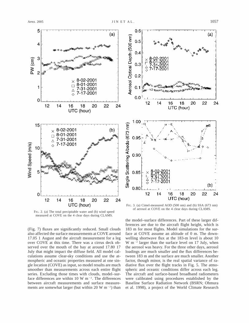
Figure 1 shows temperature and water vapor profilesoundings at COVE on the 4 days, near Terra overpasstime. The 8-digit numbers represent the sounding timeas month, day, UTC time, and minute. Figure 2 presentsthe total PW from GPS and wind speed measured byNOAA’s instruments at COVE as a function of UTCtime for the same days. NASA Cimel instrument atCOVE provides AOD at seven wavelengths (340, 380,440, 500, 670, 870, and 1020 nm) and single scatteringalbedo (SSA) at four wavelengths (441, 673, 873, and1022 nm). Figure 3 shows the measured AOD (500 nm)and SSA (673 nm) each at one wavelength, indicatingthat the aerosol loading is much larger on 7/17 than onother days. Aerosol scattering phase functions are alsoavailable from AERONET at four wavelengths, but tem-poral coverage is sparse.
Some ocean parameters were measured in situ duringCLAMS. Figure 4 shows averages of the spectral ab-sorption coefficients measured at COVE during CLAMS

1056 VOLUME 62J O U R N A L O F T H E A T M O S P H E R I C S C I E N C E S — S P E C I A L S E C T I O N
FIG. 1. The (a) temperature and (b) water vapor profiles measured at COVE on the 4 clear days during CLAMS. The 8-digit numbersrepresent the sounding time in order of month, day, UTC time, and minute.
for CDOM (which is soluble, rather than particulate),phytoplankton (a subset of the particulate matter) andall particles. These measurements indicate that the ab-sorption from ocean materials (other than H2O) atCOVE is dominated by CDOM for wavelengths lessthan 400 nm, while it is mainly contributed by partic-ulates for wavelengths longer than 600 nm. There are87 measurements of chlorophyll concentration inCLAMS. Chlorophyll indicates the phytoplankton bio-mass in seawater and is the principal parameter used inbio-optical models to parameterize the absorption andscattering by ocean particles (Morel 1991). The meanmeasured chlorophyll concentration in surface waters atCOVE is 1.33 mg m23, while a standard deviation of0.9 mg m23 demonstrates substantial variability. Theabsorption peaks of chlorophyll at around 440 and 670nm are seen in the absorption spectrum for phytoplank-ton presented in Fig. 4. All these atmospheric and oce-anic properties measured at the corresponding times areused in model simulations of radiation in the followingsection.
b. Comparisons between measurements and model
1) BROADBAND SHORTWAVE
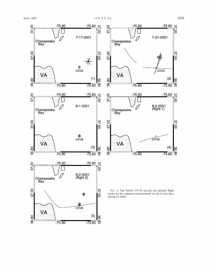
Figure 5 shows the NASA OV-10 aircraft flight trackswith special low-altitude (183 and 31 m) measurementsof broadband fluxes during the 4 clear days at CLAMS.The circle represents the location of the ChesapeakeLighthouse—the COVE site (36.9058N, 275.7138E)—
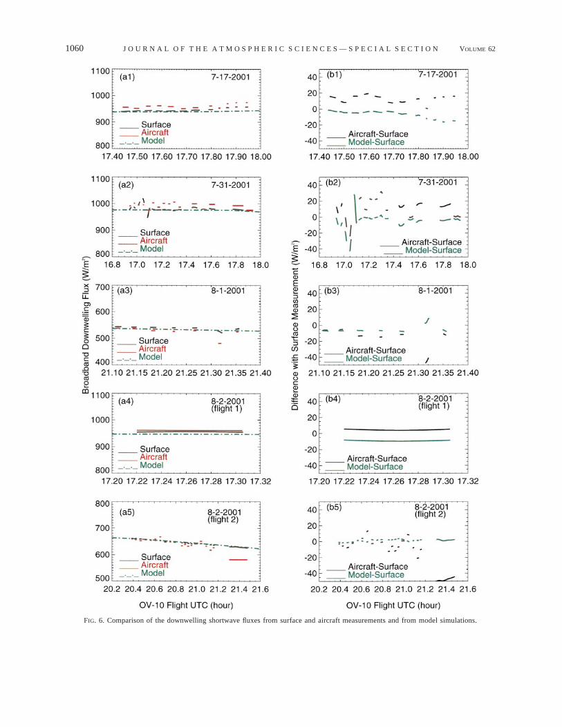
which is also the center of the CLAMS experiment do-main. Each of the five panels (Fig. 5) represents a seriesof flight legs over the ocean, and each solid line rep-resents the level portion of a flight leg. There were twoflights, each with a distinct panel, on 2 August 2001.Corresponding to the flight legs in each panel in Fig.5, Fig. 6 compares the measured and modeled downwardshortwave fluxes (irradiances). Figure 6 includes fluxesfor the COVE platform, as well as for the aircraft: Figs.6a1–6a5 show the fluxes themselves; Figs. 6b1–6b5show the respective differences of aircraft and surface(COVE) measurements, and then the differences of themodel and surface measurements. Most aircraft datawere taken 183 m above the ocean; a few legs were at31 m. Figures 6a1 to 6a5 and Figs. 6b1 to 6b5 corre-spond with the five panels in Fig. 5, respectively. Theabscissa in Fig. 6 gives the flight time in UTC and eachsection of the solid lines corresponds in time to a flightleg in the respective panel in Fig. 5. The aircraft data(red lines in Figs. 6a1 to 6a5) are averaged for each leg.The dashed–dotted lines in Fig. 6 are model resultsbased on the input parameters described in section 4a.To remove the solar zenith dependence, results in eachpanel are normalized to the solar zenith at the start ofeach flight series. The effects of changing solar zenithangle are small here, except for flight 2 on 2 August(Fig. 6a5), which has the longest flight time.
Occasionally, clouds contaminated the measurements,as seen in the leg at 21.32 1 August and 21.30 2 August,for which both the downwelling (Fig. 6) and upwelling
APRIL 2005 1057J I N E T A L .
FIG. 2. (a) The total precipitable water and (b) wind speedmeasured at COVE on the 4 clear days during CLAMS.
FIG. 3. (a) Cimel-measured AOD (500 nm) and (b) SSA (673 nm)of aerosol at COVE on the 4 clear days during CLAMS.
(Fig. 7) fluxes are significantly reduced. Small cloudsalso affected the surface measurements at COVE around17.05 1 August and the aircraft measurement for a legover COVE at this time. There was a cirrus deck ob-served over the mouth of the bay at around 17.80 17July that might impact the diffuse field. All model cal-culations assume clear-sky conditions and use the at-mospheric and oceanic properties measured at one sin-gle location (COVE) as input, so model results are muchsmoother than measurements across each entire flightseries. Excluding those times with clouds, model–sur-face differences are within 10 W m22. The differencesbetween aircraft measurements and surface measure-ments are somewhat larger (but within 20 W m22) than
the model–surface differences. Part of these larger dif-ferences are due to the aircraft flight height, which is183 m for most flights. Model simulations for the sur-face at COVE assume an altitude of 0 m. The down-welling shortwave flux at the 183-m level is about 10W m22 larger than the surface level on 17 July, whenthe aerosol was heavy. For the three other days, aerosolloadings are much smaller and the flux differences be-tween 183 m and the surface are much smaller. Anotherfactor, though minor, is the real spatial variance of ra-diative flux over the flight tracks in Fig. 5. The atmo-spheric and oceanic conditions differ across each leg.The aircraft and surface-based broadband radiometerswere calibrated using procedures established by theBaseline Surface Radiation Network (BSRN; Ohmuraet al. 1998), a project of the World Climate Research

1058 VOLUME 62J O U R N A L O F T H E A T M O S P H E R I C S C I E N C E S — S P E C I A L S E C T I O N
FIG. 4. The average spectral absorption coefficients of ocean ma-terials measured at COVE during CLAMS. The dashed–dotted lineis for pure water. Note factor of 10 scale for both curves representingthe effects of suspended particulates.
Program (WCRP). The discrepencies shown in Fig. 6fall within established instrument uncertainties for aglobal pyranometer (3%–5%).
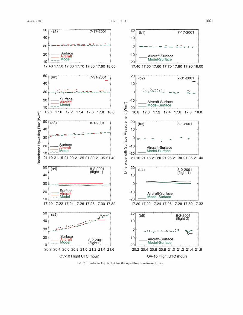
Figure 7 is similar to Fig. 6, but for the upwellingshortwave fluxes. In Fig. 7, the aircraft-measured up-welling fluxes for the leg around data point 17.9 31 Julyare substantially larger than other legs in the same flightseries. This leg traversed the mouth of the ChesapeakeBay (in the corresponding panel of Fig. 5, the western-most leg). The water properties at the mouth were dif-ferent from those under other legs. Specifically, themouth has more scattering particles (e.g., sediments inthe water) that reflect more radiation. This ocean effectwill be further explored in a later section. On the sameday, the effect of flight altitude on the upwelling fluxis also visible in the aircraft data in Fig. 7. The threelegs between 17.4 and 17.7 on 31 July are only 31 mabove the ocean, lower than the other legs (183 m) inthe same flight series. The upwelling fluxes and thedifferences for the three low-level flights are apparentlysmaller than other legs in the same flight series due toless atmospheric scattering. Excluding those cloud af-fected times, most model–surface differences in the up-welling flux are within 2 W m22, but they are somewhatlarger for the time corresponding to the flight 2 in thelate afternoon on 2 August, when solar zenith was largeand upwelling flux was more sensitive to surface rough-ness or wind speed. Similar to the downwelling flux,the aircraft–surface differences are also larger than themodel–surface differences for most legs. Those factorsaffected the aircraft downwelling flux and discussedabove also affect the upwelling flux measurements andcontribute to the discrepancies.
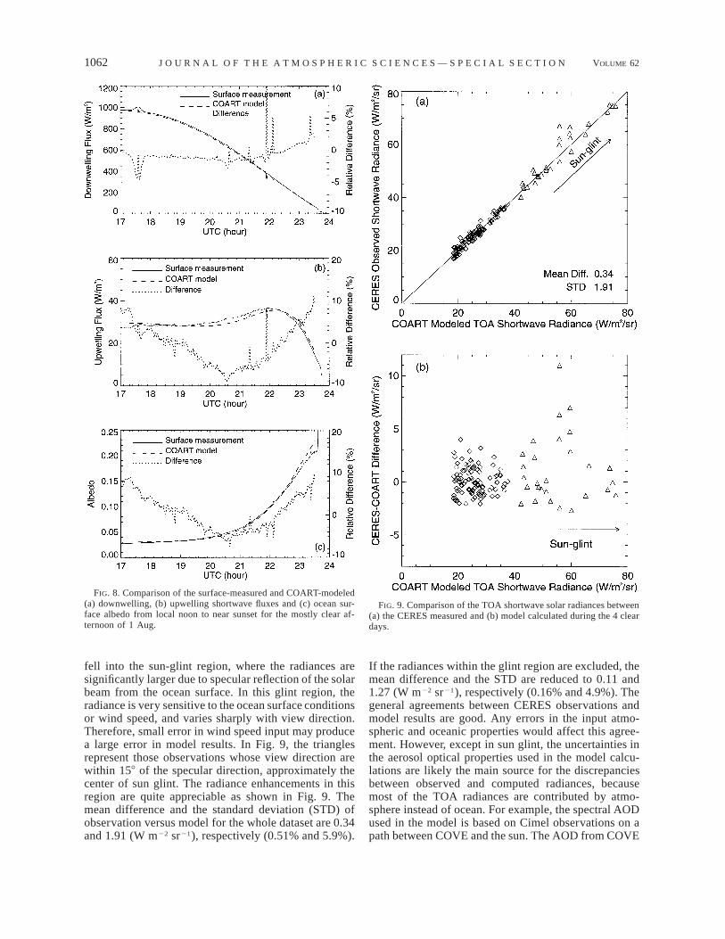
Figure 8 compares the surface-measured (solid lines)and modeled (dashed lines) downwelling and upwellingbroadband fluxes and albedo from local noon to nearsunset for a mostly clear afternoon of 1 August. Morning
observations of upwelling flux at COVE are not usedbecause of shading by the platform. The dotted linesrepresent the relative differences between model andmeasurement. Again, model calculations assume clear-sky conditions and, if cloudy, use aerosol propertiesmeasured during the nearest adjacent clear interval. Thisfigure shows that the solar zenith dependences for thedownwelling and upwelling fluxes are very different.Unlike the downwelling flux, the surface upwelling fluxfor clear conditions does not decrease monotonicallywith solar elevation; there is a peak at around 2200 UTC.This is because the ocean surface albedo increases assolar elevation decreases, and this compensates for thedecreased incidence at the surface due to a smaller solarelevation. The relative differences in downwelling fluxfor clear conditions are within 2%. They are within 10%for upwelling fluxes and albedo. The upwelling fluxmeasured around noon (1700 UTC) is still affected (re-duced) by the shadow of the lighthouse frame on thesea. In the late afternoon, the impact of the shadow onthe measurement becomes minute, and the measurementnoise itself is higher.
Discrepancies between modeled and observed fluxescan be caused by an inadequate radiative transfer model,incorrect inputs to the model, or even observation errors.The aerosol SSA and phase function in the broadbandcalculations depend on the aerosol model (Hess et al.1998), because Aeronet SSA and phase function havevalues at only four wavelengths and are too sparse intemporal coverage. We regard the largest source of mod-el–observation discrepancy for downwelling surfaceflux to be the inputs for aerosol optical properties in themodel. The model error in the downwelling flux willalso be transferred to the upwelling flux. Most discrep-ancies in the upwelling fluxes, however, are likely fromincorrect input of ocean optical properties and windspeed. Measurements of ocean optical properties duringCLAMS are not as intensive and complete as for theatmospheric properties.
2) COMPARISONS WITH CERES TOAMEASUREMENTS
Terra passed COVE at about 1600 UTC each dayduring CLAMS. One (of two) CERES instruments wasswitched to a specially programmed scanning mode thatincreased the frequency of measurements at COVE byan order of magnitude. Figure 9a compares the CERESdirectly observed shortwave solar radiances at top ofatmosphere (TOA; Wielicki et al. 1996) with those mod-eled based on the atmospheric and oceanic propertiesmeasured in situ at COVE for the 4 clear days duringCLAMS. Figure 9b shows the radiance difference be-tween CERES and model versus the TOA radiance.Only those MODIS cloud-screened ocean footprintswhose centers were within 15 km of COVE are selectedfor the comparison (Minnis et al. 2003). View zenithangles range from about 128 to 618. Many observations
APRIL 2005 1059J I N E T A L .
FIG. 5. The NASA OV-10 aircraft low-altitude flighttracks for the radiation measurements on the 4 clear daysduring CLAMS.
1060 VOLUME 62J O U R N A L O F T H E A T M O S P H E R I C S C I E N C E S — S P E C I A L S E C T I O N
FIG. 6. Comparison of the downwelling shortwave fluxes from surface and aircraft measurements and from model simulations.
APRIL 2005 1061J I N E T A L .
FIG. 7. Similar to Fig. 6, but for the upwelling shortwave fluxes.
1062 VOLUME 62J O U R N A L O F T H E A T M O S P H E R I C S C I E N C E S — S P E C I A L S E C T I O N
FIG. 8. Comparison of the surface-measured and COART-modeled(a) downwelling, (b) upwelling shortwave fluxes and (c) ocean sur-face albedo from local noon to near sunset for the mostly clear af-ternoon of 1 Aug.
FIG. 9. Comparison of the TOA shortwave solar radiances between(a) the CERES measured and (b) model calculated during the 4 cleardays.
fell into the sun-glint region, where the radiances aresignificantly larger due to specular reflection of the solarbeam from the ocean surface. In this glint region, theradiance is very sensitive to the ocean surface conditionsor wind speed, and varies sharply with view direction.Therefore, small error in wind speed input may producea large error in model results. In Fig. 9, the trianglesrepresent those observations whose view direction arewithin 158 of the specular direction, approximately thecenter of sun glint. The radiance enhancements in thisregion are quite appreciable as shown in Fig. 9. Themean difference and the standard deviation (STD) ofobservation versus model for the whole dataset are 0.34and 1.91 (W m22 sr21), respectively (0.51% and 5.9%).
If the radiances within the glint region are excluded, themean difference and the STD are reduced to 0.11 and1.27 (W m22 sr21), respectively (0.16% and 4.9%). Thegeneral agreements between CERES observations andmodel results are good. Any errors in the input atmo-spheric and oceanic properties would affect this agree-ment. However, except in sun glint, the uncertainties inthe aerosol optical properties used in the model calcu-lations are likely the main source for the discrepanciesbetween observed and computed radiances, becausemost of the TOA radiances are contributed by atmo-sphere instead of ocean. For example, the spectral AODused in the model is based on Cimel observations on apath between COVE and the sun. The AOD from COVE

APRIL 2005 1063J I N E T A L .
FIG. 10. Comparison of the TOA shortwave upwelling fluxes between CERES and model.
to satellite may be different, especially if the view zenithangle is large, due to potential horizontal variability ofaerosol. In addition, aerosol properties measured atCOVE are limited to a few individual wavelengths in-stead of covering the whole solar spectrum as CERES.The different surface coverages in size and locationfrom different view angles also contribute to the dif-ferences. Model calculations assume a uniform surfacewith no clouds. Unscreened clouds would increase ob-served radiances and fluxes, relative to those modeled.
Figure 10 shows the CERES- and model-derived up-welling TOA fluxes over COVE as a function of CERESmeasurement time day by day for the 4 clear days inCLAMS. Figures 10a1 to 10a4 are for CERES fluxes,and Figs. 10b1 to 10b4 are for model-derived fluxes.Figures 10c1 to 10c4 show the sun-glint angles for allobservations. The sun-glint angle is defined as the anglebetween the satellite view direction and the speculardirection of solar beam. A smaller glint angle corre-sponds to a larger sun-glint effect. Those observations
1064 VOLUME 62J O U R N A L O F T H E A T M O S P H E R I C S C I E N C E S — S P E C I A L S E C T I O N
with sun-glint angle less than 208 are shown as redtriangles in Fig. 10.
Like any other satellite observations, CERES TOAflux must be obtained through the conversion of CERESradiance. CERES TOA fluxes in Figs. 10a1 to 10a4 areestimated from the broadband radiances shown in Fig.9 by dividing the radiances with anisotropic factors thataccount for the angular dependence of the radiance.These anisotropic factors are predetermined empiricalangular distribution models (ADMs) that are constructedfrom 9 months of CERES/Tropical Rainfall MeasuringMission (TRMM) cloud-free ocean observations and de-pend on surface wind speed and aerosol optical depth(Loeb and Kato 2002); the version of CERES Terraused here is CERpSSFpTerra-FM2-MODISpEdition1A.The model-derived fluxes (Figs. 10b1 to 10b4) are alsoconverted from the same CERES-observed radiancesthrough the same procedure used for CERES flux con-version, but use different anisotropic factors. The mod-el-derived fluxes use the anisotropic correction factorsfrom the TOA radiance distribution calculated byCOART from the in situ measured atmospheric and oce-anic properties. Because no direct TOA flux measure-ments can be used to compare and check the CERES-or model-derived fluxes converted from radiances,COART is then used to calculate the TOA fluxes again,but here with the usual Gaussian quadrature integrationof radiances from discrete ordinates (and correspondingin time to CERES radiance measurements by using thosein situ measurements at COVE as input); these fluxesare plotted as dotted lines in Fig. 10. Because constantinputs are used, and the solar zenith angle varies littlefor a single satellite overpass, the directly calculatedTOA fluxes are basically the same in each day. Themean differences between the derived and the COARTcalculated fluxes, and the STDs of these differences arealso shown in Fig. 10. Results in Fig. 10 show that boththe CERES- and model-derived fluxes from radiancesare distributed around the model-calculated values. TheCERES-derived fluxes are similar to the model-derivedfluxes on 31 July and 1 August, but CERES fluxes havewider spread on 17 July and 2 August, because manyobservations are affected by sun glint in these 2 days.When an observation is made in the vicinity of sun glint,the anisotropic factor used for radiance to flux conver-sion becomes sensitive to wind speed. CERES here usesEuropean Centre for Medium-Range Weather Forecasts(ECMWF) wind speed with four intervals for its ADM.The model-derived fluxes use in situ–measured wind atCOVE. The unphysical low fluxes from CERES on 17July and 2 August are from the observations with smallsun-glint angle. They are overcorrected for the aniso-tropic effect, possibly due to the incorrect wind speedsapplied.
For each day, the CERES observations (which spe-cially target COVE at several different view angles ina single pass) were made within a very few minutes;the center of each was within 15 km of COVE; all were
carefully screened for clouds. Ideally, if the atmosphereand ocean were homogeneous horizontally and theocean state did not vary during the satellite overpass,the TOA fluxes should produce nearly a single valuefor each overpass. However, it is obvious that the de-rived TOA fluxes are distributed within a range for eachday. There are several factors causing the spread in de-rived fluxes. One is the inhomogeneity of the actualatmospheric properties, especially aerosol, and the spa-tial and temporal variation of the oceanic properties,especially the surface condition (e.g., the wind-drivensurface roughness). The CERES observations here in-volve a wide range of view angles, which results in verydifferent footprint sizes and coverages. They cover dif-ferent areas of coastal waters, which may have differentreflectances. Some of them with large view angle mayeven include small pieces of land in the field of view.Another important factor is error in the anisotropic fac-tor used to convert radiance to flux as described above,especially for those view directions with small sun-glintangle. Though independent ADMs are applied, the var-iations of the CERES- and model-derived fluxes aresimilar on 31 July (Figs. 10a2 and 10b2) and on 1 Au-gust (Figs. 10a3 and 10b3), in which the sun-glint anglesare large for the observations. This indicates that thevariability of the fluxes derived from observations withsmall sun-glint effects is mainly from the actual vari-ation of the radiances observed from different anglesdue to the inhomogeneity of the atmospheric, surfaceand oceanic properties.
3) OBSERVED AND MODELED SPECTRAL ALBEDO
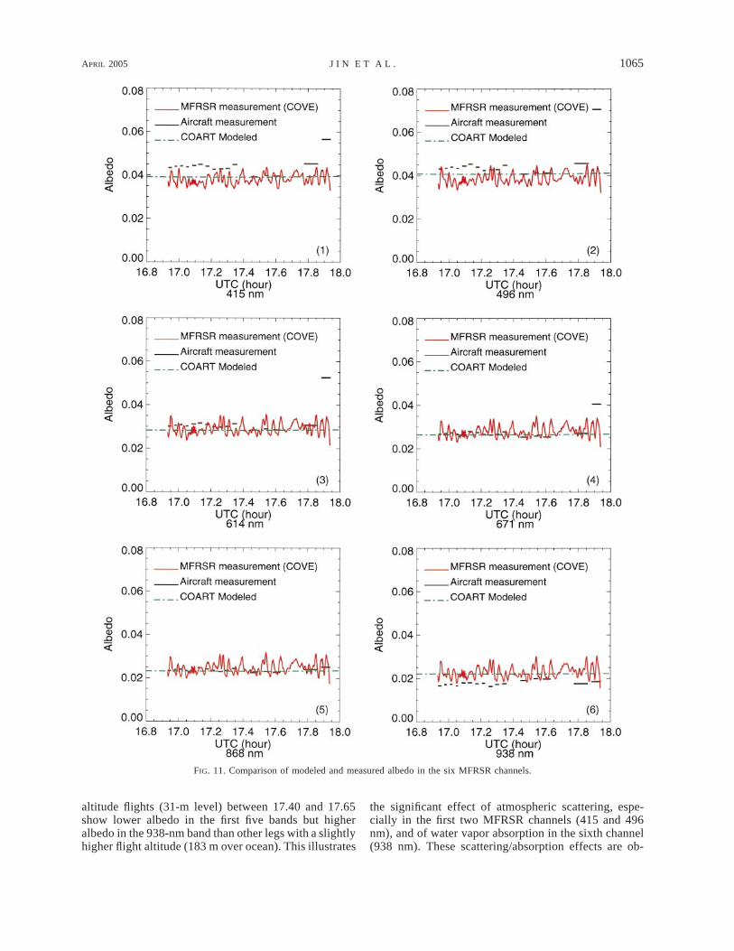
Figure 11 shows a comparison between the measuredand modeled surface albedo in the six MFRSR channelson 31 July. The solid lines are MFRSR measurementsat COVE and the dashed–dotted lines are model resultsbased on the input parameters presented above. Theblack solid lines represent the measurements (leg av-erage) from the OV-10 aircraft on the flight tracks shownin Fig. 5 (top right) for 31 July. To remove the relativedifference between the two instruments and obtain ac-curate ocean surface albedo, the two surface-basedMFRSR instruments used for the downwelling and up-welling irradiance measurements were calibrated rela-tive to each other in advance, by observing the sametarget at the same time. The mean calibration ratios fromthese measurements in each channel are applied to themeasured albedo calculations of Fig. 11. A similar pro-cedure was also applied to the two field spectrometersaboard the OV-10 and applied to the data presented here.
The rapid variations in MFRSR albedo in Fig. 11 arelikely due to changes of the ocean surface (i.e., waves),rather than underlight, because those albedo variationsare similar in all the six channels. The aircraft mea-surements were affected by the flight altitude, the hor-izontal variability of the atmospheric, surface and oce-anic properties, and even the calibration. The three low-
APRIL 2005 1065J I N E T A L .
FIG. 11. Comparison of modeled and measured albedo in the six MFRSR channels.
altitude flights (31-m level) between 17.40 and 17.65show lower albedo in the first five bands but higheralbedo in the 938-nm band than other legs with a slightlyhigher flight altitude (183 m over ocean). This illustrates
the significant effect of atmospheric scattering, espe-cially in the first two MFRSR channels (415 and 496nm), and of water vapor absorption in the sixth channel(938 nm). These scattering/absorption effects are ob-

1066 VOLUME 62J O U R N A L O F T H E A T M O S P H E R I C S C I E N C E S — S P E C I A L S E C T I O N
FIG. 12. (a) The aircraft measured albedo at seven wavelengths (b) along a flight track from A to B.Here, (b) is the SeaWiFS chlorophyll image measured 1 h after the aircraft flight.
vious even for mere 150 m of altitude difference in thelower atmosphere. The aircraft data also show signifi-cantly higher albedo for the flight leg (the last leg) thattraversed across the mouth of the Chesapeake Bay infour of the six channels, especially for the 496-nm chan-nel in which the ocean absorption is small. This supportsthe hypothesis mentioned above that there were more
scattering particle materials in the water there than inthe immediate vicinity of COVE. The particles increasedthe water reflection though the increase is too small tobe noticed in the two near-infrared channels because ofthe strong water absorption in those spectra.
To demonstrate the effect of ocean optics on surfacealbedo, Fig. 12a shows the albedo variations at six wave-
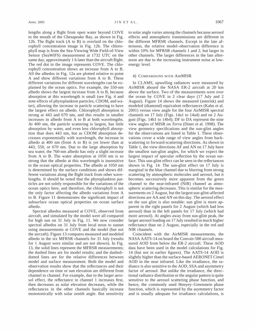
APRIL 2005 1067J I N E T A L .
lengths along a flight from open water beyond COVEto the mouth of the Chesapeake Bay, as shown in Fig.12b. The flight track (A to B) is overlaid on the chlo-rophyll concentration image in Fig. 12b. The chloro-phyll map is from the Sea-Viewing Wide Field-of-ViewSensor (SeaWiFS) measurement at 1732 UTC on thesame day, approximately 1 h later than the aircraft flight.The red dot in the image represents COVE. The chlo-rophyll concentration shows an increase from A to B.All the albedos in Fig. 12a are plotted relative to pointA and show different variations from A to B. Thesedifferent variations for different wavelengths can be ex-plained by the ocean optics. For example, the 550-nmalbedo shows the largest increase from A to B, becauseabsorption at this wavelength is small (see Fig. 4 andnote effects of phytoplankton particles, CDOM, and wa-ter), allowing the increase in particle scattering to havethe largest effect on albedo. Chlorophyll absorption isstrong at 443 and 670 nm, and this results in smallerincreases in albedo from A to B at both wavelengths.At 400 nm, the particle scattering is largest, has littleabsorption by water, and even less chlorophyll absorp-tion than does 443 nm, but as CDOM absorption de-creases exponentially with wavelength, the increase inalbedo at 400 nm (from A to B) is yet lower than at443, 550, or 670 nm. Due to the large absorption bysea water, the 760-nm albedo has only a slight increasefrom A to B. The water absorption at 1050 nm is sostrong that the albedo at this wavelength is insensitiveto the ocean optical properties. The albedo at 1050 nmis determined by the surface conditions and shows dif-ferent variations along the flight track from other wave-lengths. It should be noted that the phytoplankton par-ticles are not solely responsible for the variations of theocean optics here, and therefore, the chlorophyll is notthe only factor affecting the albedo variations from Ato B. Figure 11 demonstrates the significant impact ofsubsurface ocean optical properties on ocean surfacealbedo.
Spectral albedos measured at COVE, observed fromaircraft, and simulated by the model were all comparedfor high sun on 31 July in Fig. 11. We now considerspectral albedos on 31 July from local noon to sunsetusing measurements at COVE and the model (but notthe aircraft). Figure 13 compares measured and modeledalbedo in the six MFRSR channels for 31 July (resultsfor 1 August were similar and are not shown). In Fig.13, the solid lines represent the MFRSR measurements;the dashed lines are for model results; and the dashed–dotted lines are for the relative differences betweenmodel and surface measurement. Both the model andobservation results show that the reflectances and theirdependence on time or sun elevation are different fromchannel to channel. For example, due to the larger aero-sol effect, the reflectance in channel 1 increases first,then decreases as solar elevation decreases, while thereflectances in the other channels basically increasemonotonically with solar zenith angle. But sensitivity
to solar angle varies among the channels because aerosoleffects and atmospheric transmissions are different inthe different MFRSR channels. Except in the late af-ternoon, the relative model–observation difference iswithin 10% for MFRSR channels 1 and 2, but larger inother channels. The larger differences in the late after-noon are due to the increasing instrument noise at low-energy level.
4) COMPARISONS WITH AIRMISR
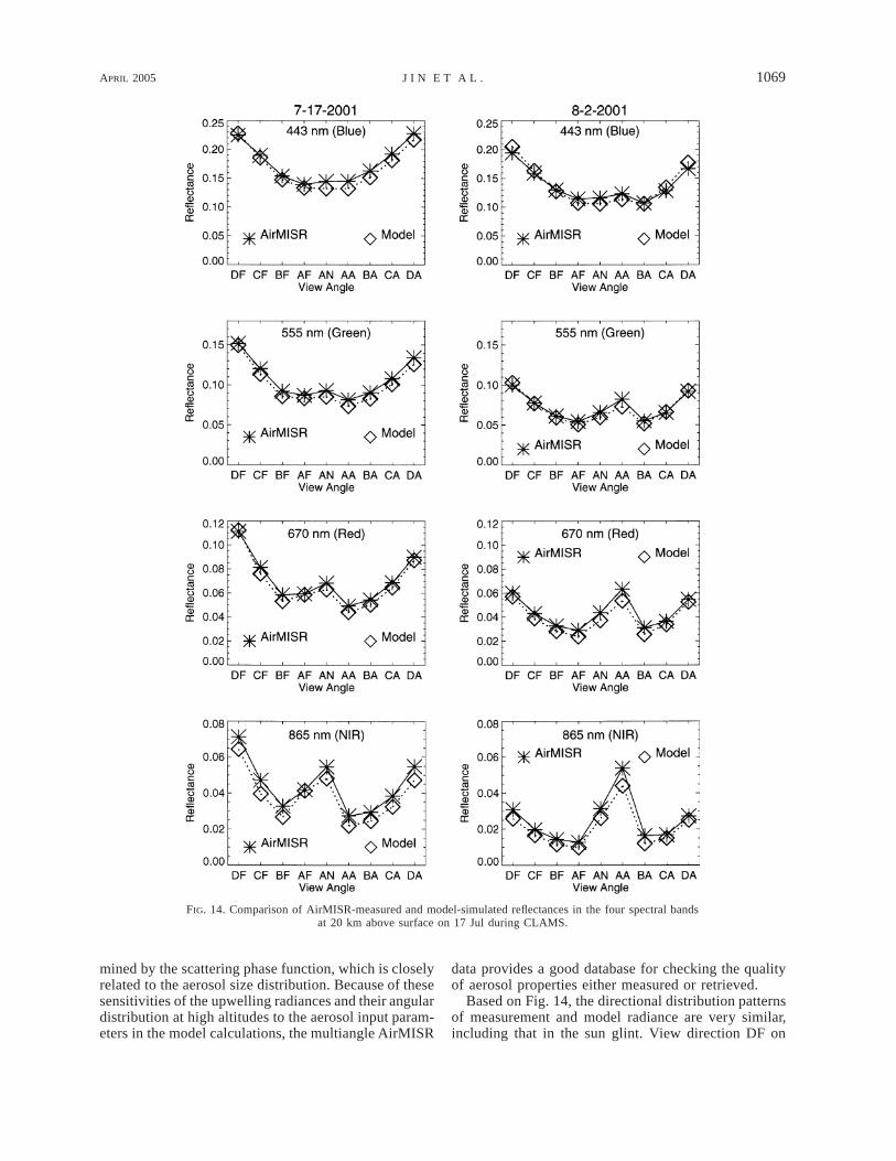
In CLAMS, upwelling radiances were measured byAirMISR aboard the NASA ER-2 aircraft at 20 kmabove the surface. Two of the measurements were overthe ocean by COVE in 2 clear days (17 July and 2August). Figure 14 shows the measured (asterisk) andmodeled (diamond) equivalent reflectances (Kahn et al.2001) versus view angle for the four AirMISR spectralchannels on 17 July (Figs. 14a1 to 14a4) and on 2 Au-gust (Figs. 14b1 to 14b4); DF to DA represent the nineview angles of MISR on Terra (Diner et al. 1998). Theview geometry specifications and the sun-glint anglesfor the observations are listed in Table 1. These obser-vations cover a wide range of view angles from back-scattering to forward-scattering directions. As shown inTable 1, the view directions AF and AN on 17 July havethe smallest sun-glint angles, for which we expect thelargest impact of specular reflection by the ocean sur-face. This sun-glint effect can be seen in the reflectancesshown in Fig. 14. The sun-glint effect on 17 July ismarginal in the blue channel due to blurring from strongscattering by atmospheric molecules and aerosol, but itbecomes successively more apparent from the greenchannel to the near-infrared (NIR) channel as atmo-spheric scattering decreases. This is similar for the mea-surements on 2 August, but the largest sun-glint-affecteddirections are AA and AN on this day. The aerosol effecton the sun glint is also notable: sun glint is more ap-parent in the right panels for 2 August (which had lessaerosol) than in the left panels for 17 July (which hadmore aerosol). At angles away from sun-glint peak, thelarger aerosol loading on 17 July resulted in much higherreflectance than on 2 August, especially in the red andNIR channels.
Coincident with the AirMISR measurements, theNASA AATS-14 on board the Convair-580 aircraft mea-sured AOD from below the ER-2 aircraft. These AODdata have been used in the model calculations for Fig.14 (but not in earlier figures). The AATS-14 AOD isslightly higher than the surface-based AERONET CimelAOD in the near infrared. Like the irradiance, the ra-diance is also sensitive to the AOD, SSA and asymmetryfactor of aerosol. But unlike the irradiance, the direc-tional radiance distribution or the angular pattern is quitesensitive to the aerosol scattering phase function, andhence, the commonly used Henyey–Greenstein phasefunction, which is represented by the asymmetry factorand is usually adequate for irradiance calculations, is

1068 VOLUME 62J O U R N A L O F T H E A T M O S P H E R I C S C I E N C E S — S P E C I A L S E C T I O N
FIG. 13. Comparison of the measured and modeled MFRSR albedo from noon to near sunset on 31 Jul 2001.
not adequate for model simulations here. An actual fullphase function has to be used to obtain a good model-observation agreement here. In other words, everythingin the aerosol optical properties, including the phase
function must be right to obtain the correct radiancesat all the very different directions as MISR. While theoverall magnitude of the MISR reflectance is sensitiveto AOD and SSA, its angular pattern is mainly deter-
APRIL 2005 1069J I N E T A L .
FIG. 14. Comparison of AirMISR-measured and model-simulated reflectances in the four spectral bandsat 20 km above surface on 17 Jul during CLAMS.
mined by the scattering phase function, which is closelyrelated to the aerosol size distribution. Because of thesesensitivities of the upwelling radiances and their angulardistribution at high altitudes to the aerosol input param-eters in the model calculations, the multiangle AirMISR
data provides a good database for checking the qualityof aerosol properties either measured or retrieved.
Based on Fig. 14, the directional distribution patternsof measurement and model radiance are very similar,including that in the sun glint. View direction DF on

1070 VOLUME 62J O U R N A L O F T H E A T M O S P H E R I C S C I E N C E S — S P E C I A L S E C T I O N
TABLE 1. AirMISR view geometry.
View angle
Sun zenith
17 Jul 2 Aug
View zenith
17 Jul 2 Aug
Relative azimuth
17 Jul 2 Aug
Sun-glint angle
17 Jul 2 Aug
DFCFBFAFAN
20.520.220.120.019.9
23.423.223.022.922.8
71.261.046.326.9
4.6
74.365.450.831.0
2.0
301.5301.6300.5296.4225.0
128.7129.6130.6131.2140.9
61.652.239.324.923.3
89.581.167.348.924.4
AABACADA
19.819.719.519.3
22.722.622.522.3
25.644.959.570.3
26.746.860.971.0
135.4131.1129.9129.9
310.9311.7312.4313.4
41.959.373.083.2
20.335.047.656.8
17 July and DA on 2 August are closest to the forwardscattering direction on each day. In these view angles,the modeled reflectances are higher than or closer to themeasurements, indicating the phase functions used heremight have a little too much forward scattering, thatmight result from the larger than actual aerosol size.Except for the forward scattering direction (i.e., DF),the modeled reflectances on 17 July are lower than theAirMISR measurements, probably because the SSAused is a little too low. The AERONET-retrieved aerosolSSA and phase function are used in the model calcu-lations here.
5. Conclusions
The comprehensive observations on the radiation andthe ancillary physical and optical properties for atmo-sphere and ocean obtained in the CLAMS experimentprovide an excellent database for validation of radiativetransfer models and remote sensing retrieval algorithms.Radiation measurements from the lighthouse tower, air-craft, and space over the ocean in the 4 clear days duringCLAMS are analyzed with the coupled radiative transfermodel (COART). The model is successively comparedwith observations of broadband fluxes and albedos nearthe ocean surface from the COVE sea platform and alow-level OV-10 aircraft, of near-surface spectral al-bedos from COVE and OV-10, of broadband radiancesat multiple angles and inferred TOA fluxes from CE-RES, and of spectral radiances at multiple angles fromAirMISR at 20-km altidude. The results show that theradiation measurements from different platforms areconsistent with each other and with radiative transfermodeling.
Clear-sky model–observation discrepancies fordownwelling shortwave flux at surface are within 10 Wm22. In most cases, model–observation discrepanciesfor upwelling shortwave flux at surface are within 2 Wm22. The model–observation discrepancies for short-wave ocean albedo are less than 8%; some discrepanciesin spectral albedo are larger but less than 20%. Thediscrepancies between low-altitude aircraft and surfacemeasurements are somewhat larger than those betweenthe model and the surface measurements; the former are
due to the effects of differences in height, aircraft pitchand roll, and the noise of spatial and temporal variationsof atmospheric, surface and oceanic properties. CERESradiances at TOA and AirMISR radiances at 20 kmabove the surface can also be well simulated by thecoupled radiative transfer model, but CERES TOA flux-es can vary significantly from model calculations forthe sun-glint affected observations. The spatial inho-mogeneity of the atmosphere and ocean have impactedthe CERES observations for the same target from dif-ferent angles, and hence, the CERES fluxes inferredfrom the radiances.
The intercomparison among measurements from dif-ferent platforms and the model show that at the surface,the uncertainties of aerosol properties are the main errorsource for the modeled downwelling fluxes; while theuncertainties of ocean surface model and ocean opticalproperties are the main error source for the modeledupwelling fluxes. Atmospheric scattering significantlyaffects the radiation in the lower atmospheric layers,especially in shortwave spectra. At the TOA and at highaltitudes, the model–observation discrepancies in thespectral and broadband upwelling radiances are mainlyfrom the uncertainties of the surface and aerosol prop-erties, including their horizontal variability. The mul-tiple angle AirMISR observations also indicate the im-portance of aerosol scattering phase function on the up-welling radiances in the upper atmosphere. In additionto the uncertainties of aerosol and ocean properties, theanisotropic correction error also affects the CERESTOA flux, especially for the observations affected bythe sun glint.
The model–observation agreements prove that mostof the observational data in CLAMS are robust, and thecoupled atmosphere–ocean radiative transfer model cor-rectly treats the scattering and absorption processes inboth the air and water. The validated data and modelcan be used to check, develop, and improve retrievalalgorithms for radiation and aerosol properties from sat-ellite data.
Acknowledgments. We thank Seiji Kato for providingus the new k-distribution data and B. N. Holben for the

APRIL 2005 1071J I N E T A L .
AERONET data. David Ruble, Xiaoju Pan, and JianWang collected the oceanographic observations.
REFERENCES
Charlock, T. P., and T. L. Alberta, 1996: The CERES/ARM/GEWEXExperiment (CAGEX) for the retrieval of radiative fluxes withsatellite data. Bull. Amer. Meteor. Soc., 77, 2673–2683.
Cox, C., and W. Munk, 1954: Measurement of the roughness of thesea surface from photographs of the sun’s glitter. J. Opt. Soc.Amer., 44, 838–850.
Diner, D. J., and Coauthors, 1998: The Airborne Multi-angle ImagingSpectroRadiometer (AirMISR): Instrument description and firstresults. IEEE Trans. Geosci. Remote Sens., 36, 1339–1349.
Dubovik, O., and M. D. King, 2000: A flexible inversion algorithmfor retrieval of aerosol optical properties from sun and sky ra-diance measurements. J. Geophys. Res., 105, 20 673–20 696.
Hess, M., P. Koepke, and I. Schult, 1998: Optical properties of aero-sols and clouds: The software package OPAC. Bull. Amer. Me-teor. Soc., 79, 831–844.
Holben, B. N., and Coauthors, 1998: AERONET—A federated in-strument network and data archive for aerosol characterization.Remote Sens. Environ., 66, 1–16.
Jin, Z., and K. Stamnes, 1994: Radiative transfer in nonuniformlyrefracting layered media: Atmosphere–ocean system. Appl. Opt.,33, 431–442.
——, T. P. Charlock, K. Rutledge, 2002: Analysis of broadband solarradiation and albedo over the ocean surface at COVE. J. Atmos.Oceanic Technol., 19, 1585–1601.
Kahn, R., P. Banerjee, D. McDonald, and J. Martonchik, 2001: Aero-sol properties derived from aircraft multi-angle imaging overMonterey Bay. J. Geophys. Res., 106, 11 977–11 995.
Kato, S., T. P. Ackerman, J. H. Mather, and E. E. Clothiaux, 1999:The K-distribution method and correlated-k approximation for
a shortwave radiative transfer Model. J. Quant. Spectros. Radiat.Trans., 62, 109–121.
Loeb, N. G., and S. Kato, 2002: Top-of-atmosphere direct radiativeeffect of aerosol over the tropical oceans from the Clouds andthe Earth’s Radiant Energy System (CERES) satellite instrument.J. Climate, 15, 1474–1484.
Minnis, P., D. F. Young, S. Sun-Mack, P. W. Heck, D. R. Doelling,and Q. Trepte, 2003: CERES Cloud Property Retrievals fromImagers on TRMM, Terra, and Aqua. Proc. SPIE 10th Int. Symp.on Remote Sensing: Conf. on Remote Sensing of Clouds and theAtmosphere VII, Barcelona, Spain, International Society for Op-tical Engineering, 37–48.
Mobley, C., and Coauthors, 1993: Comparison of numerical modelsfor computing underwater light fields. Appl. Opt., 32, 7484–7504.
Morel, A., 1991: Light and marine photosynthesis: A spectral modelwith geochemical and climatological implications. Progress inOceanography, Vol. 26, Pergamon, 263–306.
Ohmura, A., and Coauthors, 1998: Baseline Surface Radiation Net-work (BSRN/WCRP): New precision radiometry for climate re-search. Bull. Amer. Meteor. Soc., 79, 2115–2136.
Redemann, J., and Coauthors, 2005: Suborbital measurements ofspectral aerosol optical depth and its variability at subsatellitegrid scales in support of CLAMS, 200. J. Atmos. Sci., 62, 993–1007.
Smith, W. L., Jr., T. P. Charlock, R. Kahn, J. V. Martins, L. A. Remer,P. V. Hobbs, J. Redemann, and C. K. Rutledge, 2005: EOS TER-RA aerosol and radiative flux validation: An overview of theChesapeake Lighthouse and Aircraft Measurements for Satellites(CLAMS) experiment. J. Atmos. Sci., 62, 903–918.
Stamnes, K., S. C. Tsay, W. J. Wiscombe, and K. Jayaweera, 1988:Numerically stable algorithm for discrete-ordinate-method ra-diative transfer in multiple scattering and emitting layered media.Appl. Opt., 27, 2502–2509.
Wielicki, B. A., B. R. Barkstrom, E. F. Harrison, R. B. Lee, G. L.Smith, and J. E. Cooper, 1996: Clouds and the Earth’s RadiantEnergy System (CERES): An Earth Observing System experi-ment. Bull. Amer. Meteor. Soc., 77, 853–868.