Embed Size (px)
Citation preview

Radiometric Identification of Long Term EvolutionTransmitters
by
Frédéric Demers, B.Eng.
A thesis submitted to theFaculty of Graduate and Postdoctoral Affairs
in partial fulfillment of the requirements for the degree of
Master of Applied Science in Electrical and Computer Engineering
Ottawa-Carleton Institute for Electrical and Computer Engineering (OCIECE)Department of Systems and Computer Engineering
Carleton UniversityOttawa, Ontario, Canada, K1S 5B6
April, 2013
c©Copyright 2013, Frédéric Demers
The undersigned hereby recommends to theFaculty of Graduate and Postdoctoral Affairs
acceptance of the thesis
Radiometric Identification of Long Term EvolutionTransmitters
submitted by Frédéric Demers, B.Eng.
in partial fulfillment of the requirements for the degree of
Master of Applied Science in Electrical and Computer Engineering
Professor Howard Schwartz, Chair,Department of Systems and Computer Engineering
Professor Marc St-Hilaire, Thesis Supervisor
Carleton UniversityApril, 2013
ii
Abstract
This thesis investigates whether the radiometric identification of Long Term Evo-lution (LTE) transmitters is possible using commercial off-the-shelf hardware andsupport vector machine (SVM) classifiers. The identification is based on uniquemodulation characteristics exhibited by the transmitters, originating from minute im-perfections introduced during radio hardware manufacturing. In these experiments,the Agilent vector signal analysis (VSA) software and the Agilent PXA spectrumanalyzer are used to extract radiometric properties from several LTE base stations,known as evolved Node B (eNB). The open source SVM library libsvm performs theclassification using 13 emitter-specific coefficients extracted by the VSA software.
It is shown that when SVM parameters are optimized using grid search, and thetraining bin contains no less than 45 vectors, re-identification success exceeds 98% fortwo Ottawa-based providers. Furthermore, the use of feature scoring and weightingis investigated and shown to result in faster convergence for small training bins andslightly better re-identification accuracy.
iii

Acknowledgments
I would first like to express my sincere gratitude to my supervisor Professor MarcSt-Hilaire. Your accurate and rapid feedback, unfailing encouragement and personalguidance have been a source of inspiration throughout this long effort. I wish to alsothank the professors of the Ottawa-Carleton Institute for Electrical and ComputerEngineering (OCIECE) and School of Computer Science at Carleton University, whohave shown remarkable knowledge and wisdom.
Furthermore, I would like to take this opportunity to thank the dedicated membersof the Modern Communications Electronic Warfare (MCEW) team from DefenceResearch and Development Canada (DRDC) Ottawa, for supporting my researchefforts in many ways. In particular, I wish to recognize Bruce Liao and Susan Watson:I was fortunate to be able to draw on your technical knowledge and commendableexperience; your insightful advice has been precious throughout.
I also wish to recognize my many professional colleagues who exemplify some of thebest qualities the Canadian workforce has to offer. I always welcome and appreciateyour constructive feedback and support. I extend a special thanks to the managersand directors who afforded me time at critical points in my Master’s coursework andduring the writing of this thesis.
Lastly, and most importantly, I wish to dedicate this thesis to my family. ToSonia, you have spent so many days alone taking care of our daughter Annabel whilstI took time away to research, experiment and write. I cannot overstate that thisproject could not have been completed without your love and support.
To Annabel, you are a very lively and pleasant child. It has been difficult at timesto prioritize my school work instead of playing with you during your first few yearsof life. Let the completion of this thesis serve as proof that if you work hard, youtoo can realize your dreams, and remember that I will be there to help you along theway.
iv
Table of Contents
Abstract iii
Acknowledgments iv
Table of Contents v
List of Tables ix
List of Figures x
List of Acronyms xii
1 Introduction 11.1 Motivation and Applications . . . . . . . . . . . . . . . . . . . . . . . 11.2 Research Objectives . . . . . . . . . . . . . . . . . . . . . . . . . . . . 2
1.2.1 Primary Research Objectives . . . . . . . . . . . . . . . . . . . 31.2.2 Secondary Research Objectives . . . . . . . . . . . . . . . . . 3
1.3 Hypotheses . . . . . . . . . . . . . . . . . . . . . . . . . . . . . . . . 41.4 Contributions . . . . . . . . . . . . . . . . . . . . . . . . . . . . . . . 41.5 Outline . . . . . . . . . . . . . . . . . . . . . . . . . . . . . . . . . . . 5
2 Background and Literature Review 62.1 Long Term Evolution (LTE) . . . . . . . . . . . . . . . . . . . . . . . 6
2.1.1 Evolution Towards LTE . . . . . . . . . . . . . . . . . . . . . 62.1.2 LTE Downlink Characteristics . . . . . . . . . . . . . . . . . . 72.1.3 LTE Downlink Channels . . . . . . . . . . . . . . . . . . . . . 82.1.4 Orthogonal Frequency Division Multiplexing (OFDM) . . . . 102.1.5 Orthogonal Frequency Division Multiple Access (OFDMA) . . 12
v
2.2 Emitter Discrimination . . . . . . . . . . . . . . . . . . . . . . . . . . 122.3 Hardware Imperfections . . . . . . . . . . . . . . . . . . . . . . . . . 152.4 Radiometric Identification Process . . . . . . . . . . . . . . . . . . . . 15
2.4.1 Signal Acquisition . . . . . . . . . . . . . . . . . . . . . . . . . 162.4.2 Feature Extraction . . . . . . . . . . . . . . . . . . . . . . . . 162.4.3 Decision-Making Algorithms . . . . . . . . . . . . . . . . . . . 17
2.5 Transient and Steady-State Signals . . . . . . . . . . . . . . . . . . . 182.5.1 Radar Emitters . . . . . . . . . . . . . . . . . . . . . . . . . . 182.5.2 Communication Emitters . . . . . . . . . . . . . . . . . . . . . 182.5.3 Volterra Series Coefficients . . . . . . . . . . . . . . . . . . . . 192.5.4 Universal Mobile Telecommunications System . . . . . . . . . 19
2.6 Modulation Domain . . . . . . . . . . . . . . . . . . . . . . . . . . . 202.6.1 PARADIS . . . . . . . . . . . . . . . . . . . . . . . . . . . . . 202.6.2 Multiple Inputs Multiple Outputs (MIMO) Transmitters . . . 21
2.7 Reliability of Radiometric Identification . . . . . . . . . . . . . . . . . 212.8 Support Vector Machines (SVMs) . . . . . . . . . . . . . . . . . . . . 222.9 Formal Feature Selection . . . . . . . . . . . . . . . . . . . . . . . . . 262.10 Concluding Remarks . . . . . . . . . . . . . . . . . . . . . . . . . . . 28
3 Models and Theory 293.1 Radiometric Identification Features . . . . . . . . . . . . . . . . . . . 29
3.1.1 Error Vector Magnitude (EVM) . . . . . . . . . . . . . . . . . 303.1.2 EVM Peak . . . . . . . . . . . . . . . . . . . . . . . . . . . . . 303.1.3 Reference Signal EVM (RSEVM) . . . . . . . . . . . . . . . . 303.1.4 Reference Signal Transmit Power (RSTP) . . . . . . . . . . . 303.1.5 OFDM Symbol Transmit Power (OSTP) . . . . . . . . . . . . 313.1.6 Reference Signal Received Power (RSRP) . . . . . . . . . . . . 313.1.7 Reference Signal Receive Quality (RSRQ) . . . . . . . . . . . 313.1.8 Frequency Error . . . . . . . . . . . . . . . . . . . . . . . . . . 323.1.9 SYNC Correlation . . . . . . . . . . . . . . . . . . . . . . . . 323.1.10 Common Tracking Error (CTE) . . . . . . . . . . . . . . . . . 323.1.11 Symbol Clock Error . . . . . . . . . . . . . . . . . . . . . . . . 333.1.12 Time Offset . . . . . . . . . . . . . . . . . . . . . . . . . . . . 333.1.13 I&Q Offset . . . . . . . . . . . . . . . . . . . . . . . . . . . . 33
3.2 Feature Extraction and Analysis Process . . . . . . . . . . . . . . . . 34
vi
3.2.1 VSA_Interface.xlsm . . . . . . . . . . . . . . . . . . . . . . . 363.2.2 RecordingsIndex.accdb . . . . . . . . . . . . . . . . . . . . . . 383.2.3 analyze.sh . . . . . . . . . . . . . . . . . . . . . . . . . . . . . 403.2.4 looper.sh . . . . . . . . . . . . . . . . . . . . . . . . . . . . . . 423.2.5 fscore.py . . . . . . . . . . . . . . . . . . . . . . . . . . . . . . 423.2.6 mrmr . . . . . . . . . . . . . . . . . . . . . . . . . . . . . . . 453.2.7 grid.py . . . . . . . . . . . . . . . . . . . . . . . . . . . . . . . 453.2.8 weight.awk . . . . . . . . . . . . . . . . . . . . . . . . . . . . . 453.2.9 Computing Cell IDs . . . . . . . . . . . . . . . . . . . . . . . 45
3.3 Signal Quality Filtering . . . . . . . . . . . . . . . . . . . . . . . . . . 463.3.1 Signal Synchronization . . . . . . . . . . . . . . . . . . . . . . 463.3.2 Decoded Frame Number . . . . . . . . . . . . . . . . . . . . . 46
3.4 Feature Ranking and Scoring . . . . . . . . . . . . . . . . . . . . . . 473.4.1 F-score . . . . . . . . . . . . . . . . . . . . . . . . . . . . . . . 473.4.2 mRMR . . . . . . . . . . . . . . . . . . . . . . . . . . . . . . . 48
3.5 Feature Weighting and Selection . . . . . . . . . . . . . . . . . . . . . 483.6 SVM Parameters . . . . . . . . . . . . . . . . . . . . . . . . . . . . . 50
3.6.1 k-fold Cross-Validation . . . . . . . . . . . . . . . . . . . . . . 513.7 Performance Evaluation . . . . . . . . . . . . . . . . . . . . . . . . . 51
4 Results and Analysis 534.1 Experimental Procedures . . . . . . . . . . . . . . . . . . . . . . . . . 53
4.1.1 Vector Signal Analysis (VSA) . . . . . . . . . . . . . . . . . . 534.1.2 Defence Research and Development Canada (DRDC) Laboratory 544.1.3 Recordings from the City of Ottawa . . . . . . . . . . . . . . . 56
4.2 Experimental Results . . . . . . . . . . . . . . . . . . . . . . . . . . . 594.2.1 Signal Quality Filtering . . . . . . . . . . . . . . . . . . . . . 604.2.2 Variation of the Training Bin Size . . . . . . . . . . . . . . . . 614.2.3 Randomness . . . . . . . . . . . . . . . . . . . . . . . . . . . . 624.2.4 Optimization of SVM Parameters . . . . . . . . . . . . . . . . 634.2.5 Inclusion of Low Density Cells . . . . . . . . . . . . . . . . . . 654.2.6 F-score Feature Scoring and Weighting . . . . . . . . . . . . . 674.2.7 mRMR Feature Scoring and Weighting . . . . . . . . . . . . . 704.2.8 Feature Weighting Algorithms . . . . . . . . . . . . . . . . . . 734.2.9 Comparing F-score against mRMR . . . . . . . . . . . . . . . 74
vii
4.2.10 Analysis of the Impact of Adverse SNR on Re-identification . 764.2.11 Combining Cellular Providers . . . . . . . . . . . . . . . . . . 77
4.3 Analysis and Recommendations . . . . . . . . . . . . . . . . . . . . . 79
5 Conclusions and Future Work 815.1 Contributions, Results and Applications . . . . . . . . . . . . . . . . 81
5.1.1 Main Contributions and Results Overview . . . . . . . . . . . 815.1.2 Applications . . . . . . . . . . . . . . . . . . . . . . . . . . . . 82
5.2 Limitations and Recommendations . . . . . . . . . . . . . . . . . . . 835.3 Future Work . . . . . . . . . . . . . . . . . . . . . . . . . . . . . . . . 84
5.3.1 Effects of the RF Channel on Re-identification . . . . . . . . . 855.3.2 Radiometric Identification of User Equipment . . . . . . . . . 855.3.3 Other Transmitter Error Information . . . . . . . . . . . . . . 855.3.4 Emitters in Motion . . . . . . . . . . . . . . . . . . . . . . . . 865.3.5 Component Aging and Temperature . . . . . . . . . . . . . . . 865.3.6 Alternate Classifier Algorithms . . . . . . . . . . . . . . . . . 865.3.7 Principal Component Analysis . . . . . . . . . . . . . . . . . . 875.3.8 Feature Exclusion . . . . . . . . . . . . . . . . . . . . . . . . . 87
List of References 88
viii

List of Tables
2.1 Ordered significance of the features vs number of transmitters . . . . 283.1 Trace extracts file naming convention. . . . . . . . . . . . . . . . . . . 363.2 Analysis programs. . . . . . . . . . . . . . . . . . . . . . . . . . . . . 373.3 analyze.sh options. . . . . . . . . . . . . . . . . . . . . . . . . . . . . 433.4 Weighting algorithms. . . . . . . . . . . . . . . . . . . . . . . . . . . 494.1 Statistics from the recordings in the City of Ottawa 2012. . . . . . . . 594.2 Number of candidate cells as a function of filtering and number of
training vectors. . . . . . . . . . . . . . . . . . . . . . . . . . . . . . . 624.3 Sample feature scoring results using the F-score algorithm . . . . . . 684.4 Sample feature scoring results using the minimum-redundancy-
maximum-relevance (mRMR) algorithm . . . . . . . . . . . . . . . . 71
ix
List of Figures
2.1 LTE downlink channel map . . . . . . . . . . . . . . . . . . . . . . . 92.2 Spectrum of a single modulated OFDM subcarrier (truncated) . . . . 112.3 Spectrum of multiple OFDM subcarriers of constant amplitude . . . . 122.4 OFDM and OFDMA subcarrier allocation . . . . . . . . . . . . . . . 132.5 Linear hyperplane in SVM . . . . . . . . . . . . . . . . . . . . . . . . 242.6 SVM hyperplane in a higher order dimension . . . . . . . . . . . . . . 253.1 Graphical representation of modulation errors and EVM . . . . . . . 303.2 Analysis process. . . . . . . . . . . . . . . . . . . . . . . . . . . . . . 353.3 Screen capture of VSA_Interface.xlsm. . . . . . . . . . . . . . . . . . 383.4 VSA trace extraction showing feature vectors. . . . . . . . . . . . . . 393.5 Screen capture of the RecordingsIndex.accdb database. . . . . . . . . . 403.6 Geographical overlay of recording statistics. . . . . . . . . . . . . . . 413.7 Sample output of the analyze.sh processing script. . . . . . . . . . . . 444.1 Screen capture of the Agilent VSA software . . . . . . . . . . . . . . 544.2 Laboratory assembly. . . . . . . . . . . . . . . . . . . . . . . . . . . . 554.3 Cellular tower locations in Ottawa . . . . . . . . . . . . . . . . . . . . 564.4 Mobile laboratory assembly. . . . . . . . . . . . . . . . . . . . . . . . 584.5 Cellular towers in Ottawa and data gathering route . . . . . . . . . . 584.6 Prediction accuracy as a function of the number of training vectors,
randomness and signal filtering. . . . . . . . . . . . . . . . . . . . . . 604.7 Cell population as a function of the training bin size. . . . . . . . . . 614.8 Optimization of SVM parameters C and γ by grid search. . . . . . . 644.9 Prediction with SVM parameter optimization . . . . . . . . . . . . . 644.10 Prediction with and without SVM parameter optimization . . . . . . 654.11 Prediction accuracy when including cells not characterized by the SVM
model . . . . . . . . . . . . . . . . . . . . . . . . . . . . . . . . . . . 664.12 Prediction accuracy compared with and without low density cells . . 67
x
4.13 Prediction accuracy with F-score feature scoring and weighting . . . . 694.14 Prediction accuracy with F-score compared . . . . . . . . . . . . . . . 704.15 Prediction accuracy with mRMR feature scoring and weighting . . . . 724.16 Prediction accuracy with mRMR compared . . . . . . . . . . . . . . . 734.17 Prediction accuracy with F-score and feature weighting algorithms . . 744.18 Prediction accuracy with mRMR and feature weighting algorithms . . 754.19 Prediction accuracy, F-score vs mRMR . . . . . . . . . . . . . . . . . 764.20 Prediction accuracy in low signal-to-noise ratio (SNR) conditions . . . 774.21 Cell population, combined network operators . . . . . . . . . . . . . . 784.22 Prediction accuracy, combined network operators . . . . . . . . . . . 79
xi

Nomenclature
1G first generation
2G second generation
3G third generation
3GPP Third Generation Partnership Project
3GPP2 Third Generation Partnership Project 2
4G fourth generation
API application programming interface
BCH broadcast channel
BPSK binary phase shift keying
BSCD Bayesian step change detector
CDMA code division multiple access
CTE common tracking error
CSV comma-separated values
DAC digital-to-analog converter
DAG directed acyclic graph
dB decibel
DC direct current
DRDC Defence Research and Development Canada
xii
DT decision tree
eNB evolved Node B
E-UTRA evolved UMTS terrestrial radio access
EVM error vector magnitude
FDD frequency division duplexing
FFT fast Fourier transform
GLRT generalized likelihood ratio test
GSM Global System for Mobile communication
HSPA high speed packet access
HTML HyperText Markup Language
IEEE Institute of Electrical and Electronics Engineers
IMEI international mobile equipment identity
IP Internet protocol
IQ in-phase and quadrature
KLT Karhunen-Loève transformation
kNN k-nearest neighbours
LAN local area network
LDA linear discriminant analysis
LTE Long Term Evolution
MAC media access control
MCEW Modern Communications Electronic Warfare
MDL minimum description length
MIMO multiple inputs multiple outputs
xiii
mRMR minimum-redundancy-maximum-relevance
OCIECE Ottawa-Carleton Institute for Electrical and Computer Engineering
OFDM orthogonal frequency division multiplexing
OFDMA orthogonal frequency division multiple access
OSTP orthogonal frequency division multiplexing (OFDM) symbol transmit power
PARADIS Passive RAdiometric Device Identification System
PCA principal component analysis
PCI physical cell identity
PNN probabilistic neural network
PBCH physical broadcast channel
PDCCH physical downlink control channel
PDSCH physical downlink shared channel
ppm parts-per-million
PRI pulse repetition interval
PSS primary synchronization signal
QAM quadrature amplitude modulation
QPSK quadrature phase shift keying
RB resource block
RBF radial basis function
RF radio frequency
RMS root mean square
RPM revolutions per minute
RS reference signal
xiv
RSEVM received signal error vector magnitude
RSS received signal strength
RSSI received signal strength indication
RSRP reference signal received power
RSRQ reference signal received quality
RSTP reference signal transmit power
SC-FDM single-carrier frequency division multiplexing
SC-FDMA single-carrier frequency division multiple access
SEI specific emitter identification
SIM subscriber identity module
SMS short messaging service
SNR signal-to-noise ratio
SQL structured query language
SSS secondary synchronization signal
SVM support vector machine
TDD time division duplexing
TDMA time division multiple access
UE user equipment
UMB Ultra-Mobile Broadband
UMTS Universal Mobile Telecommunications System
USIM universal subscriber identity module
USRP universal software radio peripheral
VBA Visual Basic for Applications
xv

VSA vector signal analysis
VPS virtual private server
WCDMA wideband code division multiple access (CDMA)
WEKA Waikato Environment for Knowledge Analysis
WLA wireless link analysis
xvi
Chapter 1
Introduction
1.1 Motivation and Applications
The ability to uniquely identify communication emitters is essential to many defenceand security applications. Wireless service providers have a keen interest in ensuringthat only legitimate users are granted network access. This is accomplished in avariety of ways, some as simple as user authentication, or hard-coded identificationstrings provided by the user equipment (UE), which are queried against an equipmentdatabase. Since users are granted services and privileges from untethered locations,authentication is more difficult [1]. Network operators have little control over the UEwhen verifying its authenticity. The device’s hardware identification string is oftennot sufficiently reliable because it can easily be spoofed or cloned [2–4].
Conversely, users may wish to verify the access point or base station to which theyconnect legitimately belongs to the service provider, rather than a rogue device im-personating the providers’ cellular equipment. The risks of impersonation in wirelessnetwork was discussed by Barbeau et al. in [5]. A typical attack involving a rogueaccess point is further described by Hall et al. in [6], and can result in the users’ trafficbeing intercepted by the attacker.
Many modern cellular standards have struggled with cloned devices and fakedequipment identities — e.g. international mobile equipment identity (IMEI) spoof-ing, in Global System for Mobile communication (GSM). However, due to imperfectmanufacturing processes of radio frequency (RF) components, minute differences areintroduced by emitters during modulation, even for emitters of the same make andmodel. It is therefore possible to uniquely distinguish emitters by characterizing
1
CHAPTER 1. INTRODUCTION 2
aspects of the transmitted signal, a technique fittingly named radiometric identifica-tion. Radiometric identification has been demonstrated as an effective way to defeatmedia access control (MAC) address cloning in 802.11 networks, or subscriber identitymodule (SIM) card cloning in second generation (2G) cellular networks [7].
Subscriber identity in third generation (3G) or fourth generation (4G) networks iscryptographically protected and much harder to clone. In fact, the user-to-universalsubscriber identity module (USIM) link is protected by a shared secret stored securelyin the USIM or provided interactively by the user. The USIM-to-terminal link is alsoprotected by a shared secret [8]. Network operators can also detect when two userswith the same USIM parameters access the network simultaneously, ensuring this typeof attack is largely avoided. In 3G and 4G systems, the network provider equipmentmutually authenticates with the user prior to the communication taking place [9].In spite of these improvements, there are a number of practical applications whichwarrant the study of radiometric identification for the newer cellular protocols.
First, radiometric identification, also termed radio fingerprinting or specific emit-ter identification (SEI), can be used to conduct device and user tracking without thenecessity to decrypt user identification strings. The need to discover a user’s resourceblock allocation (logical-physical channel and time assignments) is also removed. Assuch, emitter tracking becomes possible for by-standers not privy to the communica-tion messaging nor encrypted identifying strings, solely recognizing the unique mod-ulation characteristics of the user’s equipment. Conversely, radiometric identificationof infrastructure emitters could help users make the determination if the base sta-tion is legitimate or is being impersonated by an attacker who may have succeededin defeating the mutual authentication. Another attack, described by Meyer andWetzel in [9], facilitates a man-in-the-middle attack to 3G handset by purposefullydowngrading the network equipment to GSM in order to bypass mutual authentica-tion. This type of attack could be prevented using properly implemented radiometricidentification. Chapter 2 presents other applications for radiometric identification inradar systems and communication systems other than Long Term Evolution (LTE).
1.2 Research Objectives
In [2], Brik et al. demonstrated a very low error rate classifying IEEE 802.11/WiFinetwork interface cards, using characteristics of the modulated signal and a support
CHAPTER 1. INTRODUCTION 3
vector machine (SVM) classifier. Classification was conducted with five parameterscollected by the Agilent vector signal analysis (VSA) software during a learning pe-riod: centre frequency offset, modulation constellation centre offset, average symbolerror vector magnitude (EVM) and phase error, and SYNC correlation. Once thelearning period was completed, the classifier algorithm attempted to match the pa-rameters collected from an unknown emitter against the classes of emitters studiedduring the learning period. Brik et al. were able to uniquely identify transmittersout of 130 WiFi cards from the same manufacturer and using the same chip set, inexcess of 99% accuracy. In this work, we wish to determine whether the modulationcharacteristics of LTE transmitters can be characterized with sufficient uniqueness asto re-establish their identity once a set of signature vectors has been gathered. Theterm radiometric identification is used henceforth to describe this activity.
1.2.1 Primary Research Objectives
The main objective of this research is to examine the suitability of the method pro-posed by Brik et al. against newer cellular communication systems and assess whetherthe re-identification success rates can be improved using a weighted classifier algo-rithm favouring the parameters with the most variance and least redundancy. Moreprecisely, we will show that unique identification of LTE emitters is possible usingthe following steps:
• Record RF signals from different LTE transmitters with an Agilent PXA spec-trum analyzer.
• Extract modulation characteristics from the recordings, for each transmitter,using the Agilent VSA software.
• Train the machine learning classifier with a subset of the parameter vectors toproduce a class model.
• Predict the identity of emitters when presented an unknown parameter vector,using the class model.
1.2.2 Secondary Research Objectives
• Determine which parameters are most effective for accurate re-identification,using two feature scoring algorithms.
CHAPTER 1. INTRODUCTION 4
• Examine the effect of parameter weighting during emitter classification andre-identification.
• Study the impact of adverse signal quality on emitter identification.
• Compare the parameters chosen by Brik et al. against those most highly rankedby the feature scoring algorithms, as a special case of feature weighting.
1.3 Hypotheses
The hypothesis is made that it is possible to collect a set of modulation characteristicsfrom an LTE base station’s downlink signal, using advanced test instrumentationsuch as a spectrum analyser with VSA capability. Once the characteristics have beenharvested, it is further hypothesized that a classifier algorithm, such as SVM, canaccurately predict the identity of an LTE emitter when presented with an unknownfeature vector. We further hypothesise that efforts towards assigning a heavier weightto the most important features will improve re-identification accuracy.
1.4 Contributions
This research activity aims to present novel contributions in the following areas:
• First successful radiometric identification of LTE transmitters using modulationcharacteristics collected by the VSA software. Many North American networkoperators have first launched LTE service during the Summer and Fall of 2011.As such, it has been challenging until now to conduct empirical research usingemitters from active 4G networks. To the best of our knowledge, this is the firstattempt at verifying this hypothesis. It is also hoped that the work completedhere will be of use for many years to come.
• First successful use of a weighted classifier algorithm such as weighted-SVMto conduct the identification. Previous radiometric identification algorithmsconsidered each feature evenly. While the success rates for IEEE 802.11/WiFias reported by Brik et al. were remarkable, it is suspected that the use ofa classifier algorithm that favours certain parameters will further enhance re-identification success rates.
CHAPTER 1. INTRODUCTION 5
• First thorough examination of the impact of adaptive modulation on re-identification. Unlike the work presented by Brik et al. in [2], LTE transmittershave the ability to adapt their modulation between quadrature phase shift key-ing (QPSK), 16 quadrature amplitude modulation (QAM) and 64 QAM in linewith the quality of the radio channel between the UE and the base station,called evolved Node B (eNB) in LTE. It may be necessary to gather radiomet-ric characteristics for each modulation schemes for re-identification to succeed.
1.5 Outline
The rest of this thesis is organized as follows. Chapter 2 provides background informa-tion useful to the reader concerning cellular standard evolution, LTE and SVMs. Thelast part of Chapter 2 provides a review of the research literature related radiometricidentification and formal feature selection. Chapter 3 provides the theoretical notionsapplied in this research effort, presents the 13 coefficients extracted from the VSA,and details the steps of the analysis process applied to the data collected. Chapter 3also presents the five weighting algorithms evaluated in this study. The empiricalresults and their significance are presented next, in Chapter 4. Finally, conclusionsand recommendations for future work are offered in Chapter 5.
Chapter 2
Background and Literature Review
This chapter presents useful background information followed by an overview of recentfindings published in research literature. Aspects of LTE protocol required to under-stand this thesis are discussed next. The necessity to conduct emitter discriminationand its most common approaches follow, along with amplifying details concerningthe source of the uniqueness present in radio signals. A discussion on the reliabil-ity of radiometric identification in real-world applications appears next. Finally, anintroduction to SVMs and a brief overview of formal feature selection concludes thechapter.
2.1 Long Term Evolution (LTE)
In this section, we provide background information that is useful for the readerthroughout this thesis. We first start by looking at the cellular network evolutionfrom first generation to today’s fourth generation. Then, we provide the reader withan introduction to LTE specifications, modulation and multiplexing schemes relevantto this study.
2.1.1 Evolution towards Long Term Evolution
Research work for the 2nd generation of mobile communication systems started inEurope in the early 1980s, and the complete system was ready for market in 1990.The most successful 2G system, called GSM is based upon time division multipleaccess (TDMA) in which eight users share a single narrowband radio channel. InNorth-America, service providers chose for the most part the competing code division
6
CHAPTER 2. BACKGROUND AND LITERATURE REVIEW 7
multiple access (CDMA) standard. These 2G systems replaced the 1st generationanalogue cellular systems.
Due to the limited throughput offered by 2G systems, several research efforts weremade in order to develop a third generation of cellular networks. Universal MobileTelecommunications System (UMTS) was the predominant 3G standard globally andstarted commercial implementation around 2002 [10]. North-American network op-erators mostly opted for CDMA-2000 services but many converted at some point tothe UMTS or its high speed packet access (HSPA)-based extensions.
Compared with earlier GSM networks, these UMTS systems provide much higherdata throughput, typically in the range of 64 to 384 kbit/s, while the peak data ratefor low mobility or indoor applications approaches 2Mbit/s. With the improvementsoffered by HSPA, data rates of up to 7.2Mbit/s are available in the downlink [10].
When UMTS was designed, the air interface was specified with a carrier band-width of 5MHz. Wideband CDMA (WCDMA), the air interface chosen at that time,performed very well within this limit. Unfortunately, WCDMA does not scale well.If the bandwidth of the carrier is increased to sustain higher transmission speeds, thetime between two transmission steps, or symbols, has to decrease. This results intransmissions being more vulnerable to multipath effects.
Instead of spreading one signal over the complete carrier bandwidth (e.g. 5MHz),LTE transmits the data over many narrowband orthogonal carriers of 15 kHz each.Instead of a single fast transmission, a data stream is split into many slower datastreams that are transmitted simultaneously. As a consequence, the attainable datarate compared to UMTS is similar in the same bandwidth but the multipath effect isgreatly reduced because of the longer symbol duration [11].
If less than 5MHz bandwidth is available, LTE can easily adapt and the numberof narrowband carriers is simply reduced. Several bandwidths have been specified forLTE: from 1.25MHz up to 20MHz. The channel bandwidth used in practice dependson the amount of spectrum available to the network operator. In a 20MHz band,data rates beyond 100Mbit/s can be achieved under optimal signal conditions [11].
2.1.2 LTE Downlink Characteristics
This section lists a few of the LTE characteristics that are useful for the reader tounderstand the remaining of this work, or necessary to configure the VSA softwaresettings:
CHAPTER 2. BACKGROUND AND LITERATURE REVIEW 8
• The standard LTE symbol duration is 66.7 µs. The corresponding orthogonalsubcarriers spacing is 15 kHz.
• LTE supports several channel bandwidths. Furthermore, both frequency divi-sion duplexing (FDD) or time division duplexing (TDD) are supported. Theexperiments conducted in this research activity dealt exclusively with 10MHzchannels in FDD mode. However, the conclusions drawn in Chapter 5 are be-lieved to be applicable to the other variants.
• Modulation types supported in the downlink are: binary phase shift keying(BPSK), QPSK, 16 QAM and 64 QAM. Zadoff-Chu sequences are also usedfor the primary synchronization signal (PSS) [12].
• The resource element is the smallest unit in the physical layer and occupies one15 kHz subcarrier for one symbol duration. The smallest unit in resource alloca-tion is however the resource block (RB), which occupies 12 adjacent subcarriers(180 kHz) of bandwidth during 7 symbols, or one slot [11].
• The frame structure is the same for the uplink and downlink transmission inLTE. However, the frame structure varies between FDD and TDD. The FDDframe structure is 10ms-long and contains 20 slots of 7 symbols. An LTEsubframe comprises two contiguous slots; there are therefore 10 subframes inan FDD frame, each 1ms-long [11].
• LTE supports only packet-switched communication carried by shared channels.There are therefore no dedicated channels. LTE is the first cellular standard torely exclusively on an packet-switched Internet protocol (IP)-based core networkfor both voice and data, with the exception of short messaging service (SMS),which is transported over signalling messages.
2.1.3 LTE Downlink Channels
LTE channels are defined logically. Logical channels do not occupy a specific sub-carrier frequency. Instead, certain key channels are periodically transmitted in pre-defined RBs. The others are defined in a channel map that is transmitted and an-nounces where specific logical channels are located in upcoming frames [13]. It is
CHAPTER 2. BACKGROUND AND LITERATURE REVIEW 9
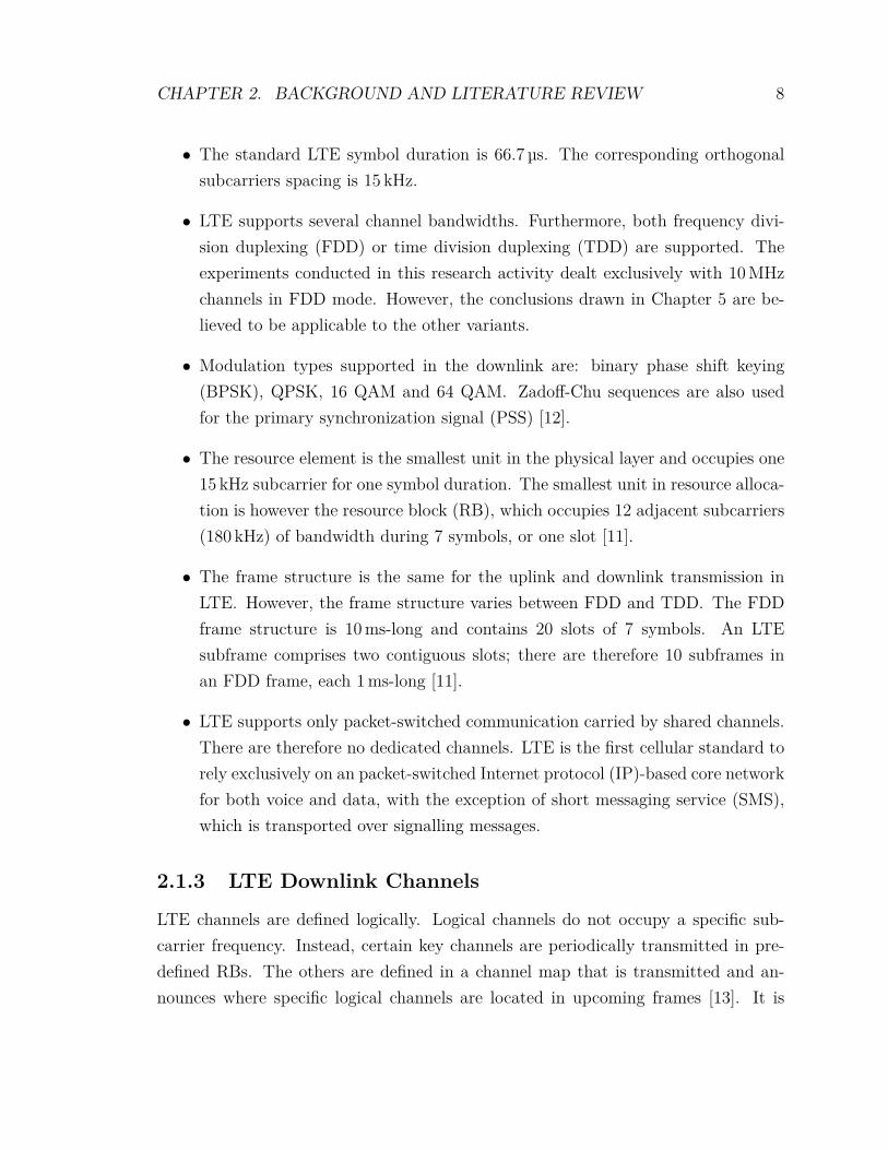
Figure 2.1: LTE downlink channel map, from [14].
important to note that logical channels are mapped to transport channels, which arein turn mapped to physical channels, as shown in Figure 2.1.
Downlink Physical Channels and Signals
This section summarizes important downlink channels and reference signals. TheUE needs to synchronize to the downlink signal before attempting to transmit andrequest to join the network [13].
PSS and SSS: The primary synchronization signal (PSS) and secondary synchro-nization signal (SSS) are two types of synchronization signals that are designedto be detected by all types of UEs. They are transmitted twice per 10ms radioframe. They occupy the central 62 subcarriers of the channel, which ensurescell search is standardized regardless of the channel bandwidth. The PSS andSSS help the UE derive the physical cell identity (PCI), a variant of which wasused as class label in the SVM classifier.
PBCH: The physical broadcast channel (PBCH) carries the broadcast channel(BCH) transport channel, which contains cell-specific content and is used forall types of UEs. It is transmitted in the centre of the channel and occupies 6RBs (72 subcarriers). It is transmitted using QPSK.
PDSCH: The physical downlink shared channel (PDSCH) carries the traffic dataand is shared in time between multiple users. QPSK, 16 QAM, and 64 QAMmodulations are supported on the PDSCH.
CHAPTER 2. BACKGROUND AND LITERATURE REVIEW 10
PDCCH: The physical downlink control channel (PDCCH) carries the channel al-location and control information. It is transmitted using QPSK.
2.1.4 Orthogonal Frequency Division Multiplexing (OFDM)
Orthogonal frequency division multiplexing is the multiplexing scheme chosen for theLTE downlink [13]. The general idea of the OFDM transmission technique is to splitthe total available bandwidth B into many narrowband sub-channels at equidistantfrequencies. The sub-channel spectra overlap each other but the subcarrier signals arestill orthogonal. The single high-rate data stream is subdivided into many low-ratedata streams for the sub-channels. Each sub-channel is modulated individually usinga conventional modulation format such as QAM and is transmitted simultaneouslyin a superimposed and parallel form [10,13].
OFDM has the ability to perform well through a low quality channel, is immuneto frequency-selective fading and provides resistance to inter-symbol interference in amultipath environment by reducing the symbol rate transmitted on each subcarrier[13].
Since the system bandwidth B is subdivided into N narrowband sub-channels,the OFDM symbol duration TS is N times larger than in the case of an alternativesingle carrier transmission system covering the same bandwidth B. Typically, for agiven system bandwidth, the number of subcarriers is chosen in such a way that thesymbol duration TS is sufficiently large compared to the maximum multi-path delayτmax of the radio channel [10].
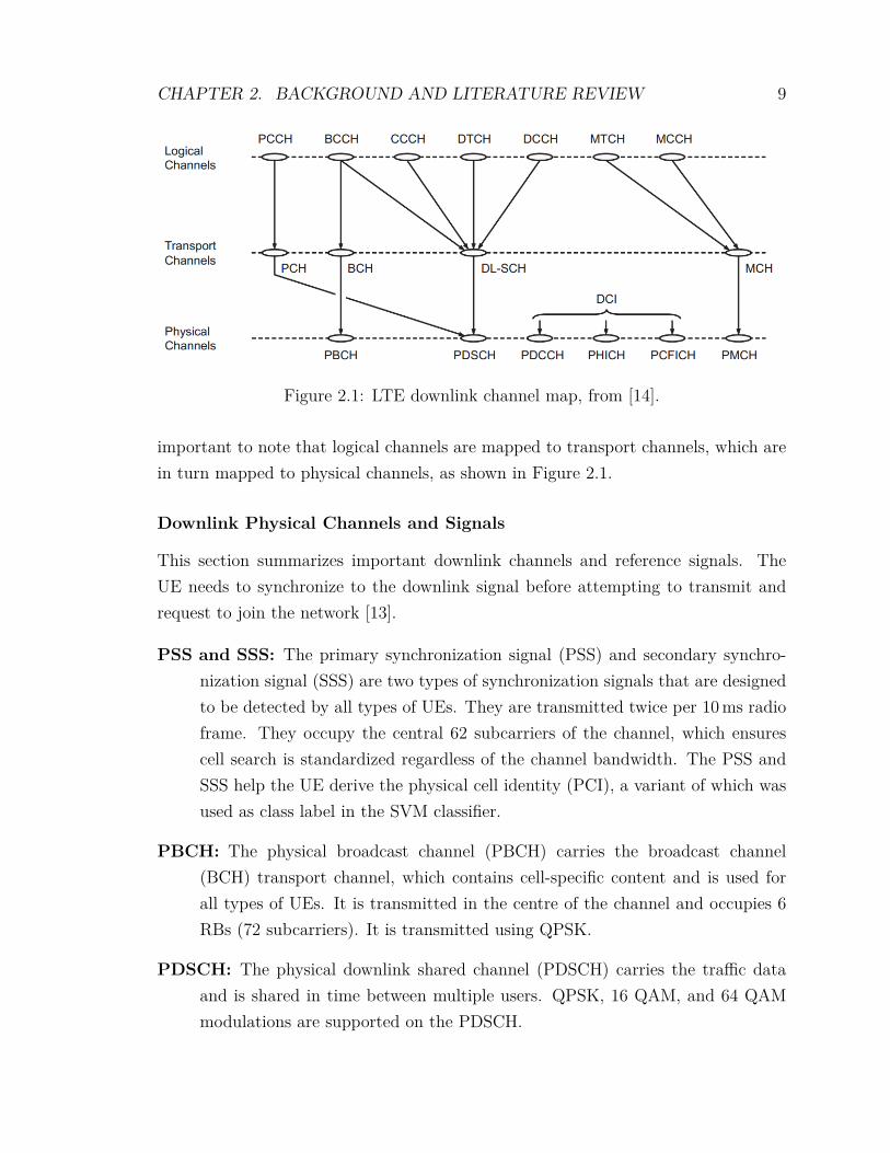
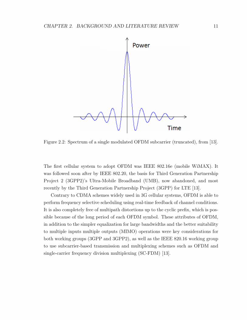
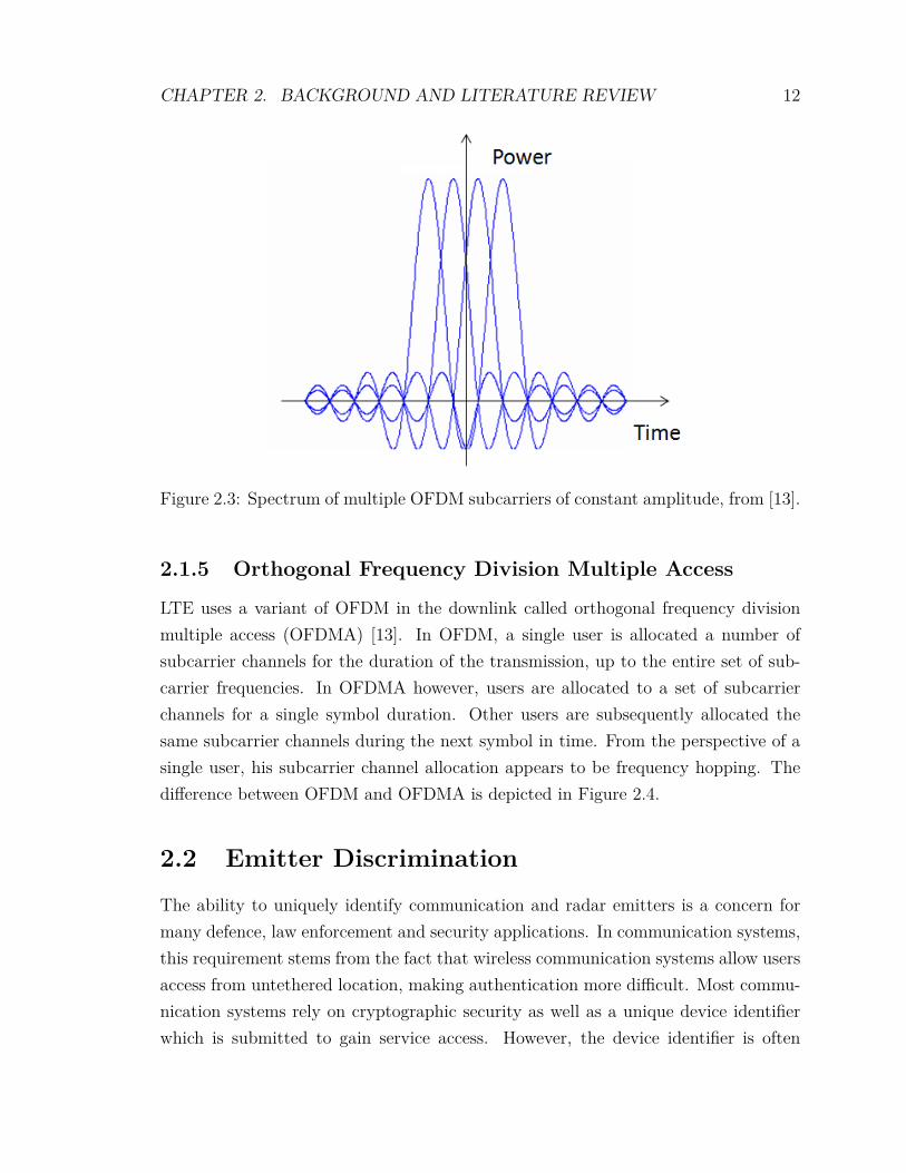
Figure 2.2 shows the power spectral density of a single OFDM subcarrier, whereasFigure 2.3 shows the power spectral density of multiple OFDM subcarriers of constantamplitude. LTE supports several constant amplitude modulation schemes that wouldresult in a power spectral density display as shown in Figure 2.3 but also supportsvariable amplitude modulation schemes such as 16 and 64 QAM [13].
Today, OFDM is widely used in applications ranging from digital television andaudio broadcasting to wireless networking such as IEEE 802.11 and wired broadbandInternet access [13, 15]. Although OFDM was considered as a candidate for GSMin the 1980s, and seriously considered again as a candidate for the UMTS standard,other multiplexing schemes were favoured due to the high cost of computing power.However, with today’s availability of small, low-cost, low-power chipsets, OFDM hasbecome the technology of choice for the next generation of cellular wireless networks.
CHAPTER 2. BACKGROUND AND LITERATURE REVIEW 11
Figure 2.2: Spectrum of a single modulated OFDM subcarrier (truncated), from [13].
The first cellular system to adopt OFDM was IEEE 802.16e (mobile WiMAX). Itwas followed soon after by IEEE 802.20, the basis for Third Generation PartnershipProject 2 (3GPP2)’s Ultra-Mobile Broadband (UMB), now abandoned, and mostrecently by the Third Generation Partnership Project (3GPP) for LTE [13].
Contrary to CDMA schemes widely used in 3G cellular systems, OFDM is able toperform frequency selective scheduling using real-time feedback of channel conditions.It is also completely free of multipath distortions up to the cyclic prefix, which is pos-sible because of the long period of each OFDM symbol. These attributes of OFDM,in addition to the simpler equalization for large bandwidths and the better suitabilityto multiple inputs multiple outputs (MIMO) operations were key considerations forboth working groups (3GPP and 3GPP2), as well as the IEEE 820.16 working groupto use subcarrier-based transmission and multiplexing schemes such as OFDM andsingle-carrier frequency division multiplexing (SC-FDM) [13].
CHAPTER 2. BACKGROUND AND LITERATURE REVIEW 12
Figure 2.3: Spectrum of multiple OFDM subcarriers of constant amplitude, from [13].
2.1.5 Orthogonal Frequency Division Multiple Access
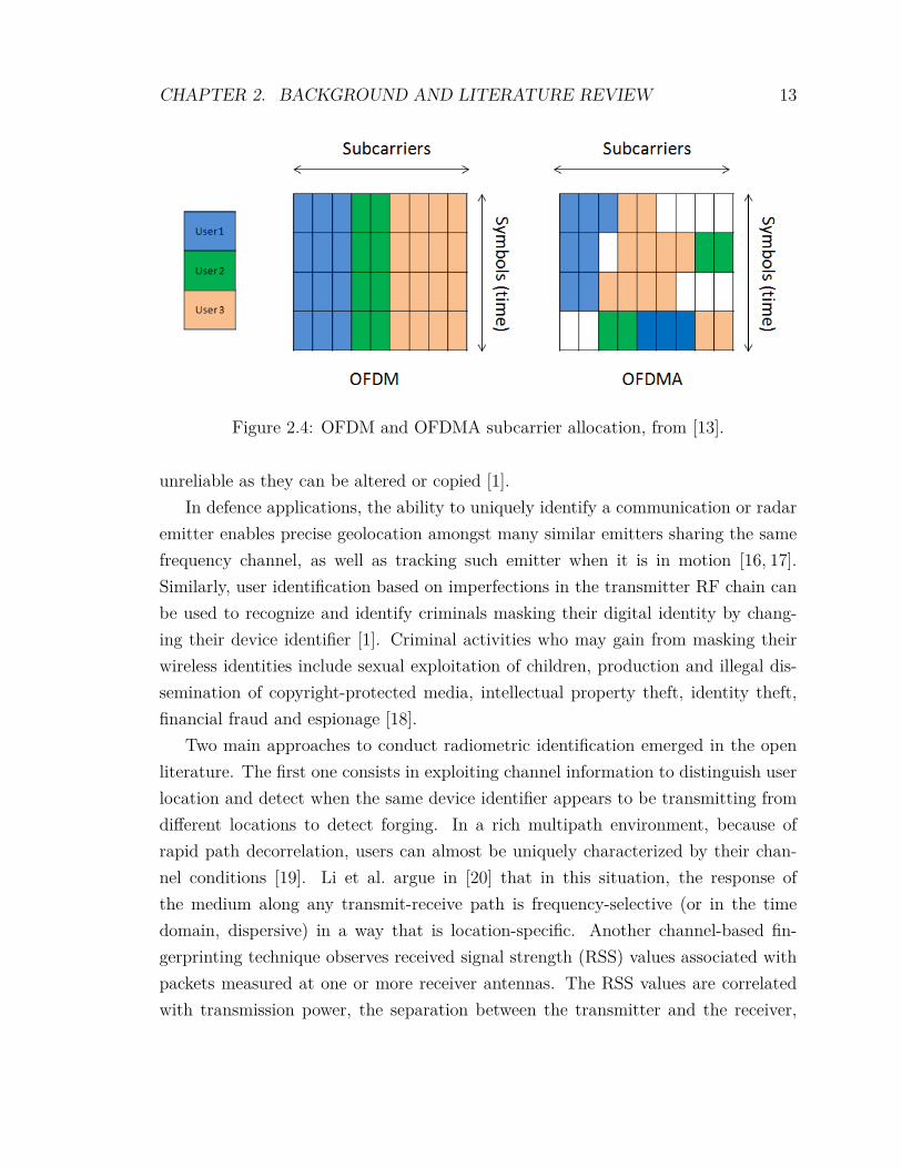
LTE uses a variant of OFDM in the downlink called orthogonal frequency divisionmultiple access (OFDMA) [13]. In OFDM, a single user is allocated a number ofsubcarrier channels for the duration of the transmission, up to the entire set of sub-carrier frequencies. In OFDMA however, users are allocated to a set of subcarrierchannels for a single symbol duration. Other users are subsequently allocated thesame subcarrier channels during the next symbol in time. From the perspective of asingle user, his subcarrier channel allocation appears to be frequency hopping. Thedifference between OFDM and OFDMA is depicted in Figure 2.4.
2.2 Emitter Discrimination
The ability to uniquely identify communication and radar emitters is a concern formany defence, law enforcement and security applications. In communication systems,this requirement stems from the fact that wireless communication systems allow usersaccess from untethered location, making authentication more difficult. Most commu-nication systems rely on cryptographic security as well as a unique device identifierwhich is submitted to gain service access. However, the device identifier is often
CHAPTER 2. BACKGROUND AND LITERATURE REVIEW 13
Figure 2.4: OFDM and OFDMA subcarrier allocation, from [13].
unreliable as they can be altered or copied [1].In defence applications, the ability to uniquely identify a communication or radar
emitter enables precise geolocation amongst many similar emitters sharing the samefrequency channel, as well as tracking such emitter when it is in motion [16, 17].Similarly, user identification based on imperfections in the transmitter RF chain canbe used to recognize and identify criminals masking their digital identity by chang-ing their device identifier [1]. Criminal activities who may gain from masking theirwireless identities include sexual exploitation of children, production and illegal dis-semination of copyright-protected media, intellectual property theft, identity theft,financial fraud and espionage [18].
Two main approaches to conduct radiometric identification emerged in the openliterature. The first one consists in exploiting channel information to distinguish userlocation and detect when the same device identifier appears to be transmitting fromdifferent locations to detect forging. In a rich multipath environment, because ofrapid path decorrelation, users can almost be uniquely characterized by their chan-nel conditions [19]. Li et al. argue in [20] that in this situation, the response ofthe medium along any transmit-receive path is frequency-selective (or in the timedomain, dispersive) in a way that is location-specific. Another channel-based fin-gerprinting technique observes received signal strength (RSS) values associated withpackets measured at one or more receiver antennas. The RSS values are correlatedwith transmission power, the separation between the transmitter and the receiver,
CHAPTER 2. BACKGROUND AND LITERATURE REVIEW 14
and the complexity of the radio environment in which communication takes place [21].However, these techniques are typically effective only in static settings, as it is well-known that RSS values can oscillate even in non-adversarial settings with legitimateusers who are mobile. In such scenarios, identification of emitters using RSS andother physical layer parameter-based solutions relying on channel information resultin a large number of false positives [21]. For these reasons, emitter discriminationbased on channel information will not be discussed further.
The second approach focuses on hardware imperfections present in each trans-mitter rather than characteristics of the radio channel. These imperfections can bestudied in the waveform domain or in the modulation domain [2]. In the waveformdomain, most research focuses on the transient portion of a signal, whether it consti-tutes a symbol in a communication system or a pulse in a radar system. A transientis a brief radio emission produced while the power of the output of an RF trans-mitter goes from zero to the level required for the application to be effective, be itcommunications, or radar detection [1]. In transient-based communication systems,efforts are made towards characterizing the transient waveform at the beginning ofeach frame. In radar systems, the physical characterization of the unintended mod-ulation of each pulse is sufficient to distinguish between radar emitters of the sameclass [22]. However, transient-based identification is more challenging for commu-nication emitters: the low transmit power and short duration of the transient isdifficult to detect, and describing the resulting waveform in a succinct way is chal-lenging [1]. Waveform-domain steady-state signal characterization was also conductedby Kennedy et al. in [23], as well as Zamora et al. [24].
On the other hand, studies of hardware imperfections in the modulation domaingenerally consists of cataloguing selected features of a communication transmitter.These features can be extracted using commercial VSA software. This techniquerepresents signals at the most basic level in terms of in-phase and quadrature (I&Q)samples, whose interpretation depends on the underlying modulation scheme. Sig-nals in the modulation domain are more structured and better behaved, but requireknowledge of the modulation scheme being used [2].
CHAPTER 2. BACKGROUND AND LITERATURE REVIEW 15
2.3 Hardware Imperfections
Due to imperfect manufacturing processes of RF components, minute differences areintroduced by emitters during modulation, even for emitters of the same make andmodel. It is therefore possible to distinguish emitters by characterizing aspects ofthe transmitted signal. Since most of this work attributes the ability to conductradiometric identification and radio-fingerprinting on hardware imperfections in thetransmitters’ RF chain, a discussion regarding the source of these imperfections iswarranted.
Each component of the transmitter chain demonstrates imperfections caused bynon-idealities of production processes. Metal-oxyde semiconductors, from which thecomponents’ circuits are made of, exhibit broad variations in major device parameters(e.g. channel length, channel doping concentration, oxide thickness) among produc-tion lots. These variations may occur for many reasons, such as minor changes in thehumidity or temperature in the clean-room, or due to the position of the die relative tothe centre of the wafer. Changes in device parameters influence transistors switchingspeed and thereby components’ characteristics. Similarly, parameters of passive elec-tronic devices follow random distributions caused by production inaccuracies, ratherthan taking a constant and uniform specified value. Despite technological advance-ments, constant market push for low-price, high-volume products results in variationsamong individual devices caused by the production imperfections. These variations,while being small enough to fulfil the requirements specified in the communicationstandards, are significant enough to allow for unique characterization of these devicesvia RF transceiverprints [1].
2.4 Radiometric Identification Process
Radiometric identification follows a similar process in the majority of open litera-ture. A training period consists of capturing the transceiverprint of the emitter.Transceiverprint gathering requires signal acquisition with sufficient precision, and isfollowed by a feature extraction. It may be necessary to extract features from severalframes or pulses during the training period in order to build a device model thatwill suitably represent typical emissions rather than a specific ones. Varying channelconditions could, for example, introduce some variance between each frame or pulsewhich may render re-identification difficult.
CHAPTER 2. BACKGROUND AND LITERATURE REVIEW 16
During the re-identification process, the signal acquisition and feature extractionis repeated for unknown devices, and the set of features is compared with knownfeatures using various decision algorithms, leading to a determination whether thedevice is recognized and provision of a confidence level [25]. Again during the re-identification, it may be necessary to extract features from several frames or pulsesin order to enhance detection reliability [2].
2.4.1 Signal Acquisition
Signal acquisition challenges vary significantly in transient-based and modulation-based approaches. In both cases, it is necessary to capture the radio signals of wire-less devices with sufficient precision. This is an important requirement given thatdevices’ fingerprints at the physical layer are due to small impairments/variations inthe devices’ radio circuitry that could be easily lost if captured with inappropriatehardware [26]. Captures in the waveform domain generally require more sensitiveequipment and are more subject to multipath and fading. Researchers operating inthe modulation domain can often use the same receiver hardware that is originallyengineered for the communication system, and demonstrate higher success rates [2].
2.4.2 Feature Extraction
The feature extraction process consists of extracting/selecting features from the radiosignal that have sufficient discriminative capabilities to distinguish a given deviceand/or a class of devices [25].
Feature extraction is more complex in transient-based systems in which a wave-form needs to be characterized. The technique employed by Shaw and Kinsner in [27]calculates the variance of the amplitude for each consecutive portion/window of thesignal and compares each of these values, in sequence, to a predetermined threshold.The start of the transient is detected when the variance exceeds the threshold by agiven margin. The end of the transient is determined in an experimental manner.The drawback of this approach is that the estimation of the threshold is difficult,given that the amplitude of the signal is susceptible to noise and interference. An-other approach, which is also based on the variance of the amplitude, is the Bayesianstep change detector (BSCD). The underlying technique, proposed by Ureten andSerinken in [28], transforms a change in the variance into a change in the mean value
CHAPTER 2. BACKGROUND AND LITERATURE REVIEW 17
that is subsequently used by the BSCD to detect the start of the transient. Un-like the previous approach, the detection of the transient is based exclusively on thecharacteristics of the amplitude data. Consequently, this approach can be used withvarious types of signals. However, the performance is less than optimal for signalsthat exhibit a gradual change in power at the start of the transient, such as IEEE802.11 and Bluetooth. The same authors have recently proposed in [29] an enhanceddetection method, referred to as the Bayesian ramp change detector to accommodatethese signals [6].
In [4], Hall et al. chose to extract features from all three main components of thetransient: amplitude, phase and frequency. The feature vectors include the standarddeviation of normalized amplitude, the standard deviation of normalized phase, thestandard deviation of normalized frequency, the variance of change in amplitude, thestandard deviation of normalized in-phase data, the standard deviation of normalizedquadrature data, the standard deviation of normalized amplitude (mean-centered),the power per section, the standard deviation of phase (normalized using mean) andthe average change in discrete wavelet transforms coefficients using the Daubechiesfilter.
In modulation-based identification, features are usually extracted using test equip-ment. In [2], Brik et al. chose five features output by the VSA software which gavebest re-identification results. Brik et al. extracted five features from each transmit-ted frame, namely frequency error, SYNC correlation, I&Q origin offset, error vectormagnitude and error vector phase [25].
2.4.3 Decision-Making Algorithms
Several algorithms can be used to find the best match between databased features,gathered during the training period, and those of an unknown emitter gathered duringthe identification period. In [2], Brik et al. demonstrated the k-nearest neighbours(kNN) as well as the SVM algorithms, with increased accuracy using the SVM.
Liu et al. compare two new online clustering algorithms that are developed forradar emitter classification in [16]: one based on the minimum description length(MDL) criterion and the other on competitive learning. The model-based algorithmis shown to surpass the competitive learning algorithm in terms of classification ac-curacy, flexibility, and stability [16].
Probabilistic neural networks (PNN) have also been used by many research teams,
CHAPTER 2. BACKGROUND AND LITERATURE REVIEW 18
however the issue of scalability (memory requirement per profile) prohibits its use inreal time systems [4]. Instead, Hall et al. favoured a statistical classifier which usesa set of features to represent a vector that is to be classified. The probability of amatch is calculated using a modified Kalman filter from Bar-Shalom.
In [18], Dolatshahi et al. consider the performance of the generalized likelihoodratio test (GLRT) and a classical likelihood ratio test to match emitters based onpower amplifiers characteristics, which features are extracted using Volterra series,with good results. GLRT outperformed the classical likelihood ratio test in mostcases.
2.5 Transient and Steady-State Signals
Radiometric identification of emitters using waveform characterization, particularlyduring the transient period, has the longest history and is still the only method bywhich radars can be discriminated.
2.5.1 Radar Emitters
In radar applications, for example, it is not difficult to distinguish radar systemswhich transmit pulses of different radio frequencies or pulse repetition interval (PRI).However, in modern radar systems, more sophisticated signal waveforms are used andinter-pulse information may not be enough to separate those received pulses accordingto their originations. To classify radar emitters in such an environment, the detailedstructure inside each pulse, called intra-pulse information, needs to be examined andcharacterized. This is because emitters exhibit their own electrical signal structureinside each transmitted pulse, due to both intentional and unintentional modulations.The SEI is a composite task that involves pulse measurements, features extraction,normalization, selection, classification (recognition) and verification [30].
2.5.2 Communication Emitters
Hall et al. published a landmark paper concerning the radiometric identification ofIEEE 802.11b communication emitters in [4]. The feature extraction and decisionalgorithms employed by Hall et al. are presented in Section 2.4.2 and Section 2.4.3.The use of a Bayesian filter, to probabilistically estimate the state of a system from
CHAPTER 2. BACKGROUND AND LITERATURE REVIEW 19
noisy observations, mitigated the increased variability between signals from a giventransceiver due to interference. The experiment consisted of collecting 100 signalsfrom each of the fourteen 802.11b transceivers. Results achieved using transient-based radio frequency fingerprinting and a Bayesian filter neared 100%.
2.5.3 Volterra Series Coefficients
In [1], Polak et al. examine the non-linearities of two components of the transmitterRF chain, namely the digital-to-analog converter (DAC) and the power amplifier, witha view to unmask the identity of criminal users. The DAC’s integral non-linearityspecifies the actual output level for a given input word, from the ideal output level, andis caused by production inaccuracies that cause output levels of individual analoguesources from the DAC to vary around their nominal values. Secondly, power amplifiersare attractive for digital forensics purposes in that they are the last elements of thetransmitter chain and are therefore the most difficult for a user to modify via softwareor even baseband control. In [1], the non-linear characteristics of power amplifierswere modelled using Volterra series representations.
In contrast with the work of Hall et al. in [4], and the work of Brik et al. in [2],the work of Polak et al. provides a complete statistics-based model which considersthe effect of signal-to-noise ratio on the probability of successful emitter recognition.
2.5.4 Universal Mobile Telecommunications System
Kennedy and Kuzminskiy present in [31] a reliable way to uniquely distinguish be-tween UMTS transmitters using steady-state characterization in the waveform do-main. The proposed algorithm differs from previous work by performing joint channelestimation and classification on a steady state signal. The technique may be appliedto any radio system with a repeated symbol sequence - such as a preamble. Thelaboratory demonstrator presented is capable of distinguishing between the preamblesignal transmitted by UMTS UEs. Excellent results - in excess of 99% for 20 dif-ferent UMTS models in an indoor wireless environment are reported. Kennedy andKuzminskiy also comment on the work of Brik et al. in [2] as the frequency offseterror between transmitter and receiver dominates the discriminatory performance oftheir solution. Whilst frequency offset applies to 802.11, it is not easily applicable toUMTS and other systems where the handset constantly disciplines its local timing
CHAPTER 2. BACKGROUND AND LITERATURE REVIEW 20
source to the base station broadcast channels. The much tighter front-end specifica-tions for frequency offset and error vector magnitude of UMTS handsets also maketheir discrimination a more difficult problem than the 802.11 case. The raw mea-surement data was first collected using a Rohde and Schwarz FSQ26 signal analyser,then processed in Matlab. The processing stage involved locating and extracting thepreamble bursts and filtering out any preambles of lower power that may have beencaptured, from multipath. The coherency algorithm takes the training file, compiledin an anechoic chamber, and the wireless test bursts to produce the confusion matrix.
2.6 Modulation Domain
Based on the higher identification accuracy of modulation-based transceiverprints,greater attention was devoted in reviewing publications that selected this approach.The first two papers reviewed below both performed transceiver fingerprinting ofIEEE 802.11b transmitters, a wireless data standard that uses OFDM at the phys-ical layer. Research in modulation-based radiometric identification of 4G cellulartechnologies, such as LTE, were not found. The most relevant OFDM work is thusreviewed next.
2.6.1 PARADIS
In [2], Brik et al. proposed the Passive RAdiometric Device Identification Sys-tem (PARADIS). The team conducted a modulation-based radiometric identificationusing five features provided by the VSA software, namely frequency error, SYNCcorrelation, in-phase and quadrature (IQ) origin offset, symbol magnitude error andsymbol phase error. Brik et al. achieved remarkably low radiometric identificationerror rates: using 138 unique network cards, from the same vendor and of the samemodel, they achieved an error rate of 0.34% using PARADIS with SVM classifica-tion. Invalid frames were discarded prior to the evaluation, that is frames with aninvalid checksum or those that did not comply with the 802.11b standard tolerancefor frequency and modulation error. Invalid frames accounted for 4% of the collecteddata.
CHAPTER 2. BACKGROUND AND LITERATURE REVIEW 21
2.6.2 Multiple Inputs Multiple Outputs Transmitters
Shi and Jensen present interesting results in conducting radiometric identification ofMIMO transmitters in [32]. The feature selection aspect of this research is uniqueand discussed fully in Section 2.9. Shi and Jensen were able to obtain excellent resultswith both the bagging with the decision tree (DT) kernel and SVM (in excess of 99%).They also showed that MIMO classification provides increased robustness in face ofhigh feature variance, due to the enriched feature set.
2.7 Reliability of Radiometric Identification
RF chain imperfections cannot be altered by the user without significant effort [1].However, it may be possible to reproduce another user’s identity by mimicking its RFimperfections using high-end signal generators. Danev et al. attempted, and mostlysucceeded in defeating radiometric-based identification systems in [25]. In spite of theaccepted belief that hardware imperfections are hard to reproduce, different imper-sonation attacks are proposed and demonstrated. It is shown that modulation-basedidentification can be impersonated with accuracy close to 100%. However, successfulattacks require specialized hardware and often also require a knowledge of the fea-tures that are examined and the classification algorithm. Indeed, the success rateof the impersonation highly depends on the discriminant capabilities of the classifierused [25]. The SYNC correlation, in particular, could not be accurately reproducedwith the software defined radio platform, and is also listed as one of the most reliablecriteria by Birk et al. in [2], thus a classifier which would rely heavily on this featurewould be harder to fool. In related work by Edman and Yener in [33], notable suc-cess (75%) was achieved in fooling an 802.11 radiometric identification system usingthe universal software radio peripheral (USRP), a commodity software-defined radiosystem. However, success rates only slightly above 50% were achieved when injectingsimulated packets rather than replaying sampled recordings. These attacks were alsoperformed with a-priori knowledge of the recognition features.
Transient-based features could also be reproduced with a high-end arbitrary wave-form generator over a wire, but the attacks were largely unsuccessful over the wirelessmedium. This is due to channel multipath effects on the transient part of the sig-nal. Feature extraction at the receiver will differ from those of the attacker tryingto clone because the channel effects will vary between the pairs attacker-receiver and
CHAPTER 2. BACKGROUND AND LITERATURE REVIEW 22
transmitter-receiver [25].The complexity involved in conducting a successful impersonation attack against
a system which discriminates based on physical-layer behaviour is two-fold. 1) Theattacker requires specialized hardware to capture the target device’s signal, not unlikethe one of the system under attack. 2) The attacker also requires the specializedhardware needed to reproduce features of this signal with sufficient fidelity to foolthe security system. Danev et al. conclude in [25] that physical-layer identification is,alone, not a suitable technique to enforce access policy and that other authenticationtechniques should be used in parallel. This echoes the assessment of Brik et al. in [2].
Polak and Goeckel investigated in [19] the radiometric identification of users ac-tively trying to falsify their RF signatures by injecting slight distortion to the datasymbols. In simulations based on parameters of commercially-used power amplifiers,it is shown that the transmitter identification performance of modifying data symbolsis similar to users who are not.
2.8 Support Vector Machines
The work of Brik et al. in [2] indicate that SVMs are well suited for radiometricidentification problems, and that SVMs outperform other classifiers. Other classifiers,such as the PNN discussed by Hall et al. in [4], presented some scalability problemsrendering it difficult to use in real-time systems. As a result, the decision was madeto use the SVM classifier to validate the hypotheses. Comparing re-identificationaccuracy with other classifiers was not a research objective for this thesis, and assuch is left to Section 5.3 (Future Work). An SVM is an abstract learning machinewhich will learn from a training dataset and attempt to generalize and make correctpredictions on novel data. For the training data, we have a set of input vectors,denoted xi, with each input vector having a number m of component features. Theseinput vectors are paired with corresponding labels, which we denote yi, and thereare n such pairs (i = 1, . . . , n) [34]. The model built during training will be used topredict the correct label y for a given test vector x.
For two classes of well separated data, the learning task amounts to finding adirected hyperplane, that is, an oriented hyperplane such that data points on oneside are labelled yi = +1 and those on the other side as yi = −1. The directedhyperplane found by a SVM is intuitive: it is that hyperplane which is maximally
CHAPTER 2. BACKGROUND AND LITERATURE REVIEW 23
distant from the two classes of labelled points located on each side. The closest suchpoints on both sides have most influence on the position of this separating hyperplaneand are therefore called support vectors [34].
The separating hyperplane is given as w ·x+b = 0, in which · denotes the inner orscalar product, b is the bias or offset of the hyperplane from the origin in input space,and x are points located within the hyperplane. The normal to the hyperplane, theweight vector w, determine its orientation [34].
The SVM optimization expression is presented in Equation (2.1)
minw,b,ξ
12wTw + C
l∑i=1
ξi (2.1)
subject to: yi(wTφ (xi) + b
)≥ 1− ξi,
ξi ≥ 0
given a training set of n instance-label pairs (xi, yi), in which the feature vectorxi ∈ Rm, yi represents the class label, and where ξi is a small number, and T is thetranspose operator. Φ (·) is a mapping function allowing data points to be mappedinto a space with a different dimensionality, called feature space, with the replacementxi ·xj → Φ (xi) ·Φ (xj). C > 0 is the penalty parameter of the error term, also termedregularization parameter [34–36].
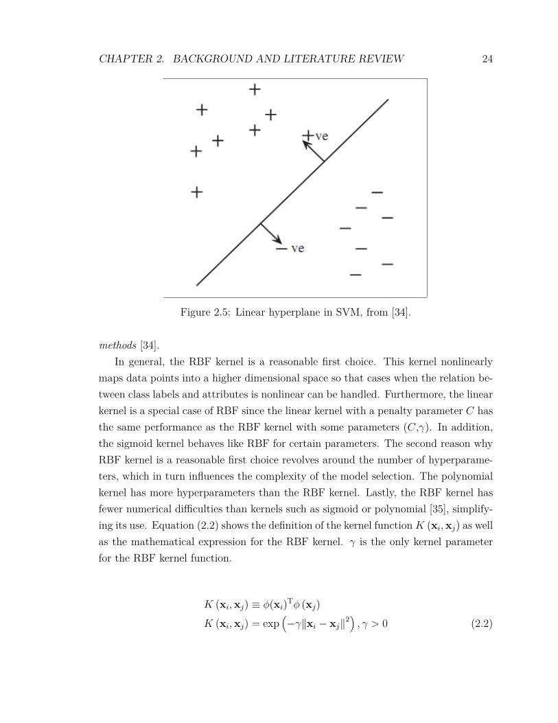
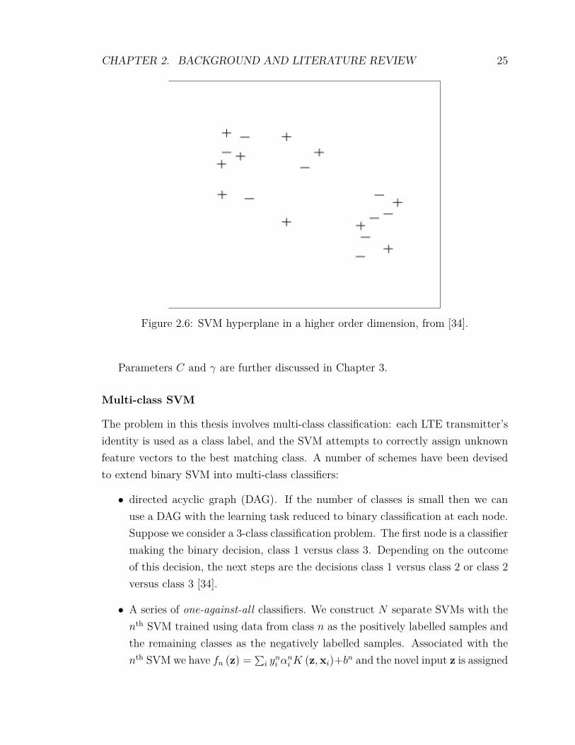
As an example Figure 2.5 shows two labelled clusters which are readily separableby a linear hyperplane. In reality, the two clusters could be highly intermeshed withoverlapping data points: the dataset is then not linearly separable, as shown in Fig-ure 2.6. Using the mapping function Φ (·), which maps the input space into a featurespace of higher dimensionality, it becomes possible to find separating hyperplanes.In Figure 2.6, which does not appear to have a linear hyperplane, if one pushes thepoints associated with one class down into a third dimension, a hyperplane couldbe readily constructed parallel to the page in order to separate the two classes [34].The hyperplanes generated by a given kernel function K (xi,xj) result in non-linearhyperplanes of various shapes once represented in the input space. Many kernel func-tions are possible, each offering different tuning parameters: polynomial, Gaussian,sigmoid, feedforward neural network or radial basis function (RBF). In fact, kernelsubstitution can be applied to a wide range of data analysis methods so that SVMsshould really be viewed as a sub-instance of a much broader class of kernel-based
CHAPTER 2. BACKGROUND AND LITERATURE REVIEW 24
Figure 2.5: Linear hyperplane in SVM, from [34].
methods [34].In general, the RBF kernel is a reasonable first choice. This kernel nonlinearly
maps data points into a higher dimensional space so that cases when the relation be-tween class labels and attributes is nonlinear can be handled. Furthermore, the linearkernel is a special case of RBF since the linear kernel with a penalty parameter C hasthe same performance as the RBF kernel with some parameters (C,γ). In addition,the sigmoid kernel behaves like RBF for certain parameters. The second reason whyRBF kernel is a reasonable first choice revolves around the number of hyperparame-ters, which in turn influences the complexity of the model selection. The polynomialkernel has more hyperparameters than the RBF kernel. Lastly, the RBF kernel hasfewer numerical difficulties than kernels such as sigmoid or polynomial [35], simplify-ing its use. Equation (2.2) shows the definition of the kernel functionK (xi,xj) as wellas the mathematical expression for the RBF kernel. γ is the only kernel parameterfor the RBF kernel function.
K (xi,xj) ≡ φ(xi)Tφ (xj)K (xi,xj) = exp
(−γ‖xi − xj‖2
), γ > 0 (2.2)
CHAPTER 2. BACKGROUND AND LITERATURE REVIEW 25
Figure 2.6: SVM hyperplane in a higher order dimension, from [34].
Parameters C and γ are further discussed in Chapter 3.
Multi-class SVM
The problem in this thesis involves multi-class classification: each LTE transmitter’sidentity is used as a class label, and the SVM attempts to correctly assign unknownfeature vectors to the best matching class. A number of schemes have been devisedto extend binary SVM into multi-class classifiers:
• directed acyclic graph (DAG). If the number of classes is small then we canuse a DAG with the learning task reduced to binary classification at each node.Suppose we consider a 3-class classification problem. The first node is a classifiermaking the binary decision, class 1 versus class 3. Depending on the outcomeof this decision, the next steps are the decisions class 1 versus class 2 or class 2versus class 3 [34].
• A series of one-against-all classifiers. We construct N separate SVMs with thenth SVM trained using data from class n as the positively labelled samples andthe remaining classes as the negatively labelled samples. Associated with thenth SVM we have fn (z) = ∑
i yni α
niK (z,xi)+bn and the novel input z is assigned
CHAPTER 2. BACKGROUND AND LITERATURE REVIEW 26
to the class n such that fn (z) is largest. Though a popular approach to multi-class SVM training, this method has some drawbacks. For example, supposethere are 100 classes with the same number of samples within each class. TheN separate classifiers would each be trained with 99% of the examples in thenegatively labelled class and 1% in the positively labelled class: these are veryimbalanced datasets, and the multi-class classifier would not work well unlessthis imbalance is addressed [34].
• One-class classification. The idea is to construct a boundary around the normaldata such that a novel point falls outside the boundary and is thus classified asabnormal. The normal data is used to derive an expression φ which is positiveinside the boundary and negative outside. One-class classification is frequentlyused for novelty detection. One-class classifiers can be readily adapted to multi-class classification. Thus we can train one-class classifiers for each class n, andthe relative ratio of φn gives the relative confidence that a novel input belongsto a particular class [34].
• One-against-one. If N is the number of classes, then N (N − 1) /2 classifiersare constructed and each one trains data from two classes. The classificationuses a voting strategy: each binary classification is considered to be a voting,where votes can be cast for all data points x - in the end a point is desig-nated to be in a class with the maximum number of votes. Hsu and Lin givein [37] a detailed comparison and conclude that one-against-one is a competi-tive approach. libsvm implements the one-against-one approach for multi-classclassification [38].
2.9 Formal Feature Selection
Whereas Birk et al. empirically determined which of the five features leads to im-proved detection accuracy in [2], Shi and Jensen provide a formal method to choosingthe VSA features based on maximum relevance and minimum redundancy. The lat-ter team determine the best classifying features for a variable number of transmittersusing the minimum-redundancy-maximum-relevance (mRMR) algorithm on the train-ing dataset, where relevance is measured by the mutual information of that featureand the device identifier h:
CHAPTER 2. BACKGROUND AND LITERATURE REVIEW 27
I (gi, h) =∫ ∑
h∈hp (gi, h) log p (gi, h)
p (gi) p (h)dgi (2.3)
where h represents the set ofNd possible values of h, and p (·) denotes the probabil-ity density function. The relevance of a set of selected features S =
g1, g2, · · · , gNf
is defined as the average of the relevance of features in the set, or
VS = 1Nf
∑gi∈S
I (gi, h) (2.4)
Similarly, redundancy is measured by the mutual information of two differentfeatures. The redundancy of the feature set is defined as the average of the mutualinformation of each pair of features in the set, or
WS = 1N2f
∑gi,gj∈S
I (gi, gj) (2.5)
Prior work on this topic has shown that finding the feature set that maximizesthe difference VS −WS is one simple approach that achieves the objective [32].
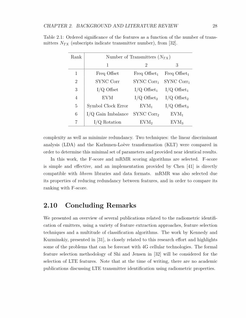
The result of their analysis is shown at Table 2.1. Interestingly, frequency offset isselected at most once even in cases with multiple transmitters. This is explained byShi and Jensen because of the likelihood that all transmitter chains use the same localoscillator and as such the frequency offset for other transmitters is highly redundant[32].
Chen and Lin examine in [39] several feature selection algorithms combined withSVMs, namely F-score, random forests and radius margin (RM)-bound SVM, andcompared against results obtained by SVM without feature selection. In the applica-tions studied, the datasets contain a very larger number of features (500 to 100 000)and feature selection reduced the number of features entering the SVM model. Theyconclude that for some problems, such as optical character recognition, the use of theSVM classifier without feature selection performs well. In other problems, greaterprediction accuracy is achieved with feature selection.
In extracting features of radar pulses, Kawalek and Owczarek discuss in [40] theset of intrapulse parameters: the rise, slope and fall time, rise angle, fall angle, angleof pulse, pulse point, frequency waveform, angle of frequency modulation, and theregression’s line. Out of these parameters, a subset is selected to reduce computational
CHAPTER 2. BACKGROUND AND LITERATURE REVIEW 28
Table 2.1: Ordered significance of the features as a function of the number of trans-mitters NTX (subscripts indicate transmitter number), from [32].
Rank Number of Transmitters (NTX)1 2 3
1 Freq Offset Freq Offset1 Freq Offset1
2 SYNC Corr SYNC Corr1 SYNC Corr1
3 I/Q Offset I/Q Offset1 I/Q Offset1
4 EVM I/Q Offset2 I/Q Offset2
5 Symbol Clock Error EVM1 I/Q Offset3
6 I/Q Gain Imbalance SYNC Corr2 EVM1
7 I/Q Rotation EVM2 EVM3
complexity as well as minimize redundancy. Two techniques: the linear discriminantanalysis (LDA) and the Karhunen-Loève transformation (KLT) were compared inorder to determine this minimal set of parameters and provided near identical results.
In this work, the F-score and mRMR scoring algorithms are selected. F-scoreis simple and effective, and an implementation provided by Chen [41] is directlycompatible with libsvm libraries and data formats. mRMR was also selected dueits properties of reducing redundancy between features, and in order to compare itsranking with F-score.
2.10 Concluding Remarks
We presented an overview of several publications related to the radiometric identifi-cation of emitters, using a variety of feature extraction approaches, feature selectiontechniques and a multitude of classification algorithms. The work by Kennedy andKuzminskiy, presented in [31], is closely related to this research effort and highlightssome of the problems that can be forecast with 4G cellular technologies. The formalfeature selection methodology of Shi and Jensen in [32] will be considered for theselection of LTE features. Note that at the time of writing, there are no academicpublications discussing LTE transmitter identification using radiometric properties.
Chapter 3
Models and Theory
This chapter first outlines the LTE radiometric properties considered for this study.Then, details concerning the feature extraction and analysis process are presented.Mathematical models for the two feature ranking and five weighting algorithms arepresented next. A discussion concerning signal quality filtering, aiming to improve re-identification accuracy, follows. Finally, an overview of the selection of a performancecriteria concludes the chapter.
3.1 Radiometric Identification Features
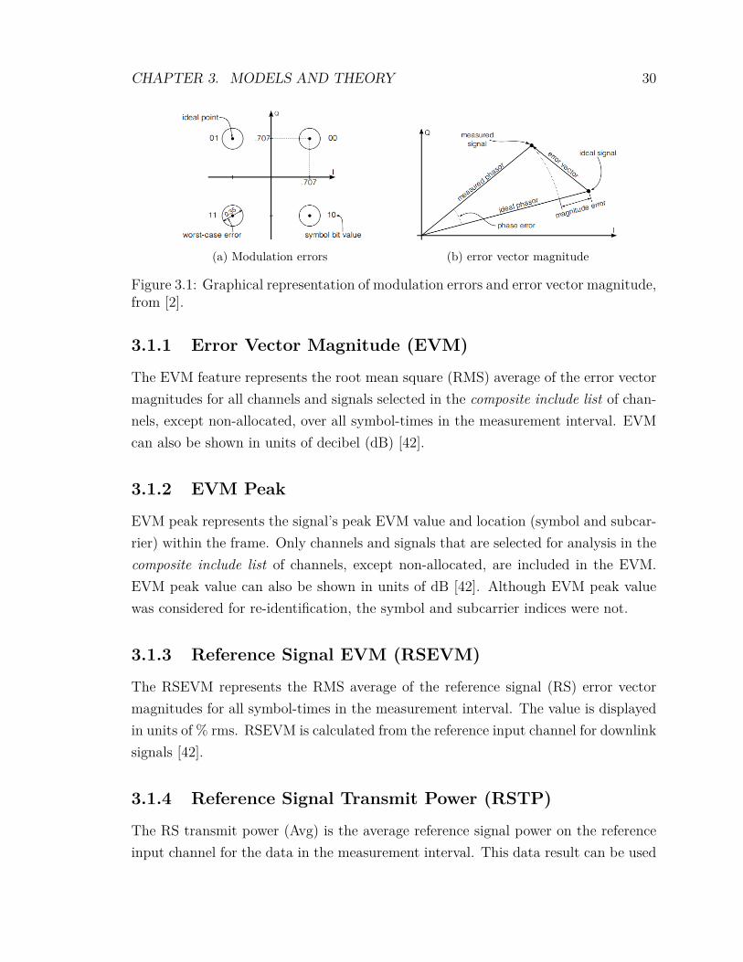
The VSA software provides several signal traces for study; however, the experimentsconducted in this thesis are centered on the Error Summary table. This decisionwas based on earlier published research by Brik et al. in [2] and the work of Shi andJensen in [32], who also used a subset of the features available on the trace of the Er-ror Summary table in their respective publications. It is also understood that traceswhich quantify RF and modulation errors are more likely to provide recognizable fea-tures originating from hardware imperfections in the RF circuitry of the transmitter.Chapter 5 presents other traces which could be studied in future research, which mayalso lead to transmitter-specific information useful for re-identification. Figure 3.1provides a graphical representation of modulation errors and the calculation of theEVM, which are important notions for the remainder of this work. The Error Sum-mary table provides the following values computed by the VSA software during theanalysis and demodulation of LTE signals.
29
CHAPTER 3. MODELS AND THEORY 30
(a) Modulation errors (b) error vector magnitude
Figure 3.1: Graphical representation of modulation errors and error vector magnitude,from [2].
3.1.1 Error Vector Magnitude (EVM)
The EVM feature represents the root mean square (RMS) average of the error vectormagnitudes for all channels and signals selected in the composite include list of chan-nels, except non-allocated, over all symbol-times in the measurement interval. EVMcan also be shown in units of decibel (dB) [42].
3.1.2 EVM Peak
EVM peak represents the signal’s peak EVM value and location (symbol and subcar-rier) within the frame. Only channels and signals that are selected for analysis in thecomposite include list of channels, except non-allocated, are included in the EVM.EVM peak value can also be shown in units of dB [42]. Although EVM peak valuewas considered for re-identification, the symbol and subcarrier indices were not.
3.1.3 Reference Signal EVM (RSEVM)
The RSEVM represents the RMS average of the reference signal (RS) error vectormagnitudes for all symbol-times in the measurement interval. The value is displayedin units of % rms. RSEVM is calculated from the reference input channel for downlinksignals [42].
3.1.4 Reference Signal Transmit Power (RSTP)
The RS transmit power (Avg) is the average reference signal power on the referenceinput channel for the data in the measurement interval. This data result can be used
CHAPTER 3. MODELS AND THEORY 31
to calculate RSTP as defined in 3GPP TS 36.141 Section F.3.3 [43]. This data resultis only applicable to downlink signals [42].
3.1.5 OFDM Symbol Transmit Power (OSTP)
The OFDM symbol transmit power is calculated by averaging the power of all resourceelements in the fourth symbol in every subframe. This is done for all subframes inthe measurement interval and over all antenna ports, as defined in 3GPP TechnicalSpecification 36.141, Section F.3.3 [43]. This data result is only applicable to downlinksignals. The fourth symbol in every subframe contains only PDSCH, so this dataresult can be interpreted as the average power of the data subcarriers. OSTP iscalculated and expressed as an absolute power in units of dB [42].
3.1.6 Reference Signal Received Power (RSRP)
The RS receive power (Avg) is a linear average of the power of all cell-specific RSresource elements from Tx antenna port 0 (and Tx port 1, when present) over thedata in the measurement interval. RSRP (Avg) can be used to calculate RSRP asdefined in Section 5.1.1 of 3GPP TS 36.214 [42,43].
When there are multiple Rx input channels present that contain transmissionsfrom Tx antenna port 0 or 1, the average RS power is calculated for each Rx inputchannel and added together to compute RS Rx Power (Avg) [42].
3.1.7 Reference Signal Receive Quality (RSRQ)
The RSRQ is a measure of the quality of the received signal as defined in Section5.1.3 of 3GPP TS 36.214 and is given by the following equation:
RSRQ = N * RSRP / (E-UTRA RSSI)where:N is the number of resource blocks over which RSRP and evolved UMTS terrestrial
radio access (E-UTRA) received signal strength indication (RSSI) are calculated (theLTE demodulator includes all resource blocks in the frame bandwidth). RSRQ iscalculated over all data in the measurement interval [42,43].
CHAPTER 3. MODELS AND THEORY 32
3.1.8 Frequency Error
The frequency error value represents the carrier frequency error relative to the VSA’scentre frequency. This parameter is displayed in Hz and is the amount of frequencyshift, from the VSA’s centre frequency, that the VSA must perform to achieve carrierlock. In the downlink, for the fast Fourier transform (FFT) demodulation, the carrierfrequency is initially determined from the preamble. The frequency error reportedin the summary table is the value from the final frequency estimation based on thechannel estimation sequence, with a fine adjustment made for any frequency errordetected in the pilot tracking. The pilot tracking does not correct the signal forfrequency errors, it only corrects the post-FFT symbols for phase (and amplitude, ifselected) [42].
3.1.9 SYNC Correlation
SYNC correlation is the correlation coefficient between the measured preamble andan ideal preamble. This can be used as an indication of the quality of the preamble.A value of 1 indicates perfect correlation and a value of 0 indicates no correlation.
Large frequency errors may cause the VSA software to show incorrect low SYNCcorrelation values. These values are a result of frequency error and do not necessarilyindicate poor signal quality. Therefore, for low SYNC correlation values you alwaysneed to validate the cause of the low SYNC correlation data result [42].
3.1.10 Common Tracking Error (CTE)
The CTE is the RMS average of the symbol-by-symbol deviation from the channel-compensated (equalized) signal expressed in % rms. An ideal signal would not have tobe tracked (no magnitude scaling or phase adjustment) and the tracking adjustmentvalue would be (magnitude 1, phase 0) for every symbol-time.
For each symbol-time in the CTE trace, the ideal signal’s CTE magnitude is sub-tracted from the measured signal’s CTE magnitude and the differences are averagedby RMS. Since the ideal signal’s CTE magnitude is 1, the calculation can be simplifiedto the equation shown below.
CTE%rms =
√√√√N−1∑t=0
(|CTEm (t)| − 1)2 × 100% (3.1)
CHAPTER 3. MODELS AND THEORY 33
where CTEm (t) is the measured common tracking error at symbol-time t, and N isthe number of symbols in the measurement interval [42].
3.1.11 Symbol Clock Error
The symbol clock error shows the frequency error between the measured signal’ssymbol clock and the reference symbol clock in parts-per-million (ppm). The erroris calculated by averaging the symbol timing corrections during the measurementinterval. The symbol clock error is calculated from the reference input channel fordownlink signals.
A value of 0.010 ppm indicates that the measured signal’s symbol clock frequencyis slower than the reference symbol clock frequency by 0.00000001×RefSymClk [42].
3.1.12 Time Offset
Shows the time offset from the beginning of the time capture to the beginning of themeasurement interval.
For example, when time offset = 5ms and the search time trace starts at −8.3ms,the beginning of the measurement interval is located at −3.3ms within the searchtime trace.
The time offset can be used to measure the accuracy of an external frame triggersignal when such signal is connected to the external trigger, the analysis start bound-ary is set to frame, and the measurement offset is set to 0. In this case, time offsetwill show the offset between the frame trigger and the actual start of the frame [42].
3.1.13 I&Q Offset
The I&Q offset indicates the magnitude of carrier feedthrough (power at 0Hz). Whenthere is no carrier feedthrough, I&Q offset is zero (-infinity dB). I&Q offset is calcu-lated by computing the RMS average of the measured I&Q offset for each symbol inthe measurement interval, and is expressed relative to the average signal power.
For a downlink signal, I&Q offset is calculated from the reference input channel.For an ideal downlink signal, any I&Q offset present would not affect the quality of thesignal since the direct current (DC) subcarrier is orthogonal to the other subcarriers.However, when the signal is impaired so that the subcarriers are not orthogonal to
CHAPTER 3. MODELS AND THEORY 34
DC (when Doppler shifted, for instance), any I&Q offset on the DC subcarrier willaffect the EVMs of other subcarriers [42].
3.2 Feature Extraction and Analysis Process
A lengthy feature extraction process was performed by the VSA software once theRF signals were recorded to disk during the field trial. The feature extraction relieson the VSA software’s LTE demodulation analysis capability. The VSA software candisplay a number of analytical traces for either live signals or recorded ones. Using theVSA application programming interface (API), it is possible to automate much of thisprocess. Specifically, with a program written in Visual Basic for Applications (VBA)(VSA_Interface.xlsm), it was possible to configure the settings of the VSA software toensure repeatability, load signal recordings, and step through extracting trace valuesfrom loaded signal recordings to generate feature vectors. The feature extraction firstpopulated a Microsoft Excel spreadsheet and was subsequently written to disk inthe comma-separated values (CSV) format. The Error Summary table was selectedfor most of the experimentation and provides several measurements taken from thesignal recording, such as EVM, SYNC correlation, symbol clock error, time offset, I&Qoffset, I&Q gain imbalance, group and cell identification strings. From observations,it became also interesting to capture other VSA status indicators such as applicationsynchronization status and raw synchronization status for every sample extracted.Another trace, the DL Decode Info, presented the decoded frame number, and thisvalue was also used to enrich the feature extraction as one additional attribute ofsignal reception quality. Lastly, the trace extraction was enhanced with the sampletime stamp. The file naming convention shown in Table 3.1 was used for all traceextracts.
A set of Linux shell scripts and simple programs were written to process the traceextracts and interface with external libraries for feature scoring and weighting, andin order to perform SVM analysis. The process flow is captured in Figure 3.2.
In all, near 10 000 SVM classification experiments were conducted. Cloud-basedcomputing resources were used to conduct the analysis, using as many as three hostedLinux virtual private server (VPS) concurrently, in order to accelerate the process.The purpose and language of each software component is summarized in Table 3.2
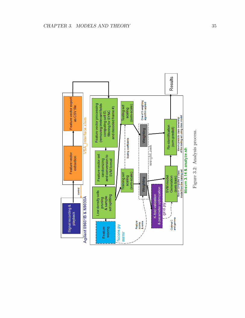
CHAPTER 3. MODELS AND THEORY 35
Figu
re3.2:
Ana
lysis
process.
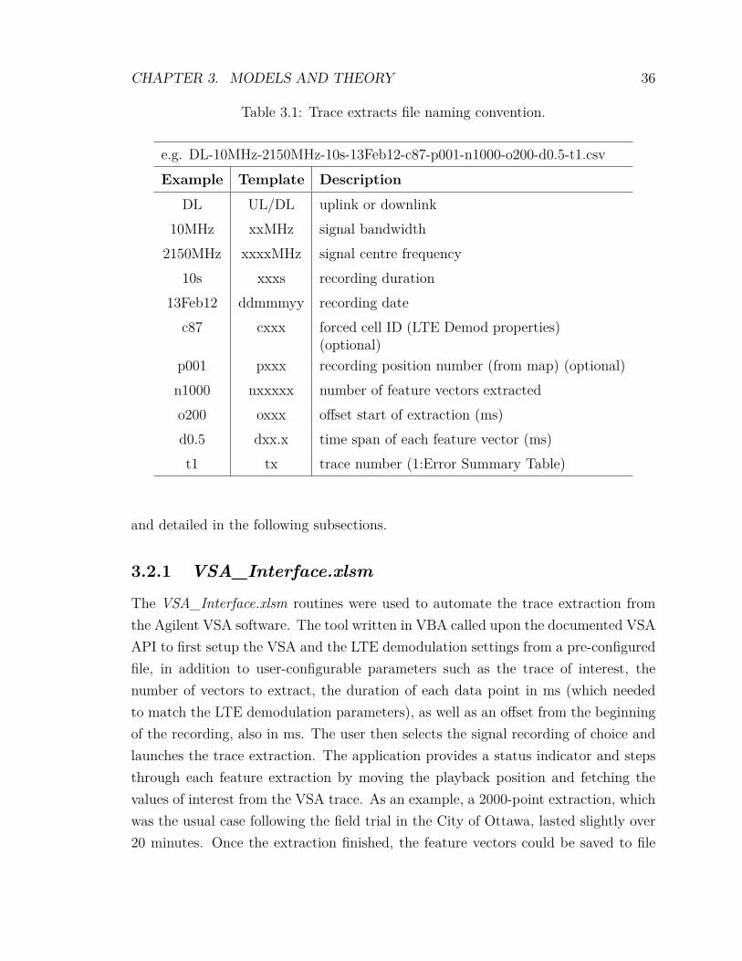
CHAPTER 3. MODELS AND THEORY 36
Table 3.1: Trace extracts file naming convention.
e.g. DL-10MHz-2150MHz-10s-13Feb12-c87-p001-n1000-o200-d0.5-t1.csvExample Template Description
DL UL/DL uplink or downlink10MHz xxMHz signal bandwidth2150MHz xxxxMHz signal centre frequency
10s xxxs recording duration13Feb12 ddmmmyy recording date
c87 cxxx forced cell ID (LTE Demod properties)(optional)
p001 pxxx recording position number (from map) (optional)n1000 nxxxxx number of feature vectors extractedo200 oxxx offset start of extraction (ms)d0.5 dxx.x time span of each feature vector (ms)t1 tx trace number (1:Error Summary Table)
and detailed in the following subsections.
3.2.1 VSA_Interface.xlsm
The VSA_Interface.xlsm routines were used to automate the trace extraction fromthe Agilent VSA software. The tool written in VBA called upon the documented VSAAPI to first setup the VSA and the LTE demodulation settings from a pre-configuredfile, in addition to user-configurable parameters such as the trace of interest, thenumber of vectors to extract, the duration of each data point in ms (which neededto match the LTE demodulation parameters), as well as an offset from the beginningof the recording, also in ms. The user then selects the signal recording of choice andlaunches the trace extraction. The application provides a status indicator and stepsthrough each feature extraction by moving the playback position and fetching thevalues of interest from the VSA trace. As an example, a 2000-point extraction, whichwas the usual case following the field trial in the City of Ottawa, lasted slightly over20 minutes. Once the extraction finished, the feature vectors could be saved to file
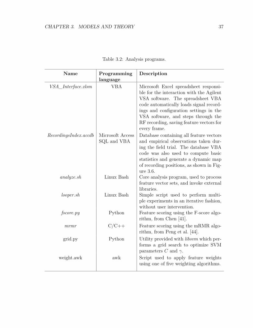
CHAPTER 3. MODELS AND THEORY 37
Table 3.2: Analysis programs.
Name Programminglanguage
Description
VSA_Interface.xlsm VBA Microsoft Excel spreadsheet responsi-ble for the interaction with the AgilentVSA software. The spreadsheet VBAcode automatically loads signal record-ings and configuration settings in theVSA software, and steps through theRF recording, saving feature vectors forevery frame.
RecordingsIndex.accdb Microsoft AccessSQL and VBA
Database containing all feature vectorsand empirical observations taken dur-ing the field trial. The database VBAcode was also used to compute basicstatistics and generate a dynamic mapof recording positions, as shown in Fig-ure 3.6.
analyze.sh Linux Bash Core analysis program, used to processfeature vector sets, and invoke externallibraries.
looper.sh Linux Bash Simple script used to perform multi-ple experiments in an iterative fashion,without user intervention.
fscore.py Python Feature scoring using the F-score algo-rithm, from Chen [41].
mrmr C/C++ Feature scoring using the mRMR algo-rithm, from Peng et al. [44].
grid.py Python Utility provided with libsvm which per-forms a grid search to optimize SVMparameters C and γ.
weight.awk awk Script used to apply feature weightsusing one of five weighting algorithms.
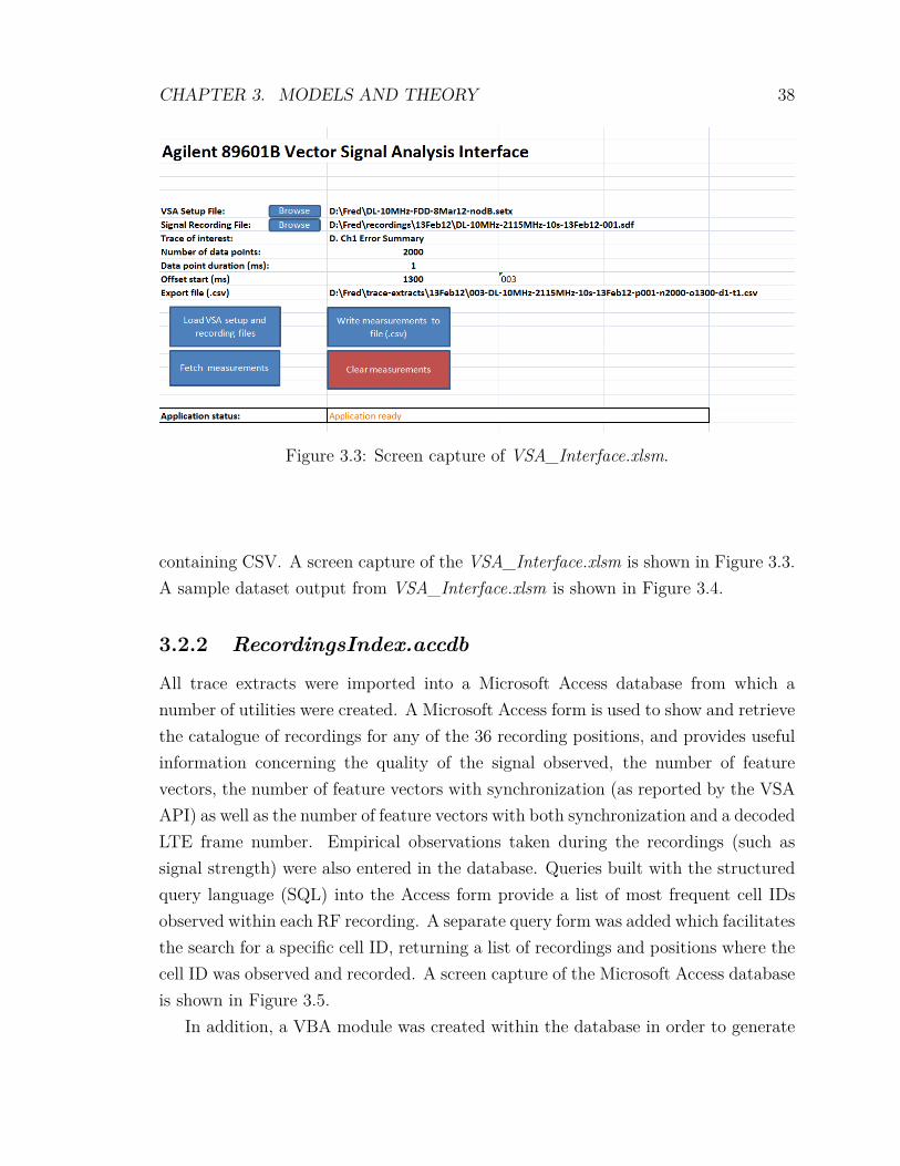
CHAPTER 3. MODELS AND THEORY 38
Figure 3.3: Screen capture of VSA_Interface.xlsm.
containing CSV. A screen capture of the VSA_Interface.xlsm is shown in Figure 3.3.A sample dataset output from VSA_Interface.xlsm is shown in Figure 3.4.
3.2.2 RecordingsIndex.accdb
All trace extracts were imported into a Microsoft Access database from which anumber of utilities were created. A Microsoft Access form is used to show and retrievethe catalogue of recordings for any of the 36 recording positions, and provides usefulinformation concerning the quality of the signal observed, the number of featurevectors, the number of feature vectors with synchronization (as reported by the VSAAPI) as well as the number of feature vectors with both synchronization and a decodedLTE frame number. Empirical observations taken during the recordings (such assignal strength) were also entered in the database. Queries built with the structuredquery language (SQL) into the Access form provide a list of most frequent cell IDsobserved within each RF recording. A separate query form was added which facilitatesthe search for a specific cell ID, returning a list of recordings and positions where thecell ID was observed and recorded. A screen capture of the Microsoft Access databaseis shown in Figure 3.5.
In addition, a VBA module was created within the database in order to generate
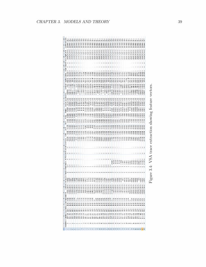
CHAPTER 3. MODELS AND THEORY 39
Figu
re3.4:
VSA
traceextractio
nshow
ingfeaturevectors.
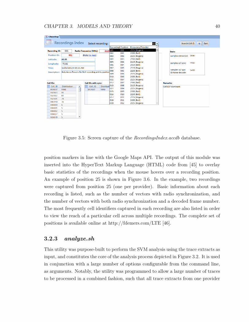
CHAPTER 3. MODELS AND THEORY 40
Figure 3.5: Screen capture of the RecordingsIndex.accdb database.
position markers in line with the Google Maps API. The output of this module wasinserted into the HyperText Markup Language (HTML) code from [45] to overlaybasic statistics of the recordings when the mouse hovers over a recording position.An example of position 25 is shown in Figure 3.6. In the example, two recordingswere captured from position 25 (one per provider). Basic information about eachrecording is listed, such as the number of vectors with radio synchronization, andthe number of vectors with both radio synchronization and a decoded frame number.The most frequently cell identifiers captured in each recording are also listed in orderto view the reach of a particular cell across multiple recordings. The complete set ofpositions is available online at http://fdemers.com/LTE [46].
3.2.3 analyze.sh
This utility was purpose-built to perform the SVM analysis using the trace extracts asinput, and constitutes the core of the analysis process depicted in Figure 3.2. It is usedin conjunction with a large number of options configurable from the command line,as arguments. Notably, the utility was programmed to allow a large number of tracesto be processed in a combined fashion, such that all trace extracts from one provider
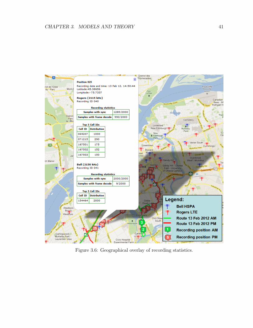
CHAPTER 3. MODELS AND THEORY 41
Figure 3.6: Geographical overlay of recording statistics.
CHAPTER 3. MODELS AND THEORY 42
could be considered as one. It further provides the ability to filter feature vectorsthat exhibited radio synchronization and/or a decoded LTE frame number. Thecommand-line options programmed into analyse.sh are listed in Table 3.3. analyze.shfirst processes the extracted feature vectors by removing unwanted columns from thetrace, computing a new unique CellID as discussed in Section 4.1.3, and performsthe filtering of vectors with synchronization and vectors with decoded frame number,as specified by the command line arguments. It then randomizes the vector set andreformats the trace according to the libsvm input format. analyse.sh then prunes cellswith too few vectors (low density cells) and splits the population of vectors between atraining set and a testing set. Scaling is the process used to normalize the numericalvalue range of each feature to ensure each feature variance is evenly considered inthe SVM model. The main advantage of scaling is to avoid attributes in greaternumeric ranges dominating those in smaller numeric ranges. Another advantage isto avoid numerical difficulties during the calculation [35]. Both sets are scaled withthe scaling factors obtained from the training set. When feature scoring is used, thefeatures are weighted by the weight.awk script, based on either rank or score outputby the chosen scoring algorithm (F-score or mRMR). Optionally, a grid search isperformed to obtain optimal SVM parameters C and γ used with an RBF kernelfunction. Lastly, the core svm-train and svm-predict programs from [45] are invokedto obtain a re-identification success rate.
3.2.4 looper.sh
A simple Linux Bash script used to run a series of analysis tasks (by analyze.sh) basedon the variables under study. This program took many forms throughout this researchactivity. The results were extracted from the looper.sh log file, a sample of which isshown in Figure 3.7, using awk, and entered into a Microsoft Excel spreadsheet fromwhich tables and graphs were generated.
3.2.5 fscore.py
fscore.py is a Python implementation of the F-score feature scoring algorithm, writtenby Chen [41]. The F-score feature scoring algorithm is discussed in Subsection 3.4.1.The script outputs three files: .fscore shows importance of features, .select gives the
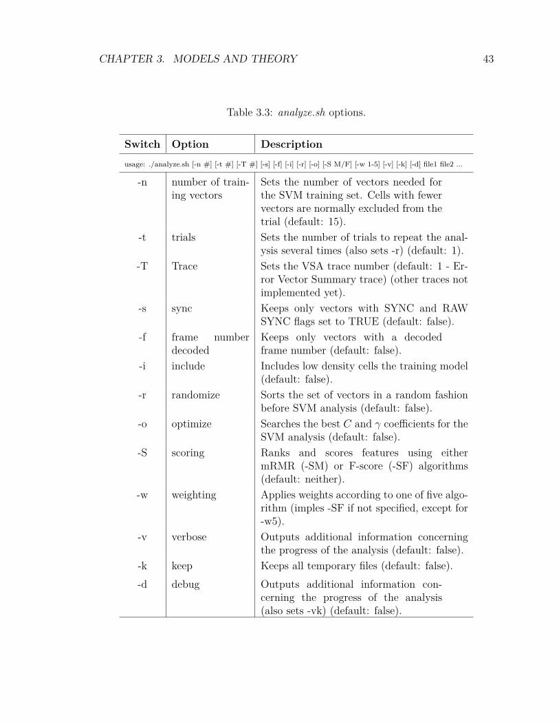
CHAPTER 3. MODELS AND THEORY 43
Table 3.3: analyze.sh options.
Switch Option Description
usage: ./analyze.sh [-n #] [-t #] [-T #] [-s] [-f] [-i] [-r] [-o] [-S M/F] [-w 1-5] [-v] [-k] [-d] file1 file2 ...
-n number of train-ing vectors
Sets the number of vectors needed forthe SVM training set. Cells with fewervectors are normally excluded from thetrial (default: 15).
-t trials Sets the number of trials to repeat the anal-ysis several times (also sets -r) (default: 1).
-T Trace Sets the VSA trace number (default: 1 - Er-ror Vector Summary trace) (other traces notimplemented yet).
-s sync Keeps only vectors with SYNC and RAWSYNC flags set to TRUE (default: false).
-f frame numberdecoded
Keeps only vectors with a decodedframe number (default: false).
-i include Includes low density cells the training model(default: false).
-r randomize Sorts the set of vectors in a random fashionbefore SVM analysis (default: false).
-o optimize Searches the best C and γ coefficients for theSVM analysis (default: false).
-S scoring Ranks and scores features using eithermRMR (-SM) or F-score (-SF) algorithms(default: neither).
-w weighting Applies weights according to one of five algo-rithm (imples -SF if not specified, except for-w5).
-v verbose Outputs additional information concerningthe progress of the analysis (default: false).
-k keep Keeps all temporary files (default: false).-d debug Outputs additional information con-
cerning the progress of the analysis(also sets -vk) (default: false).
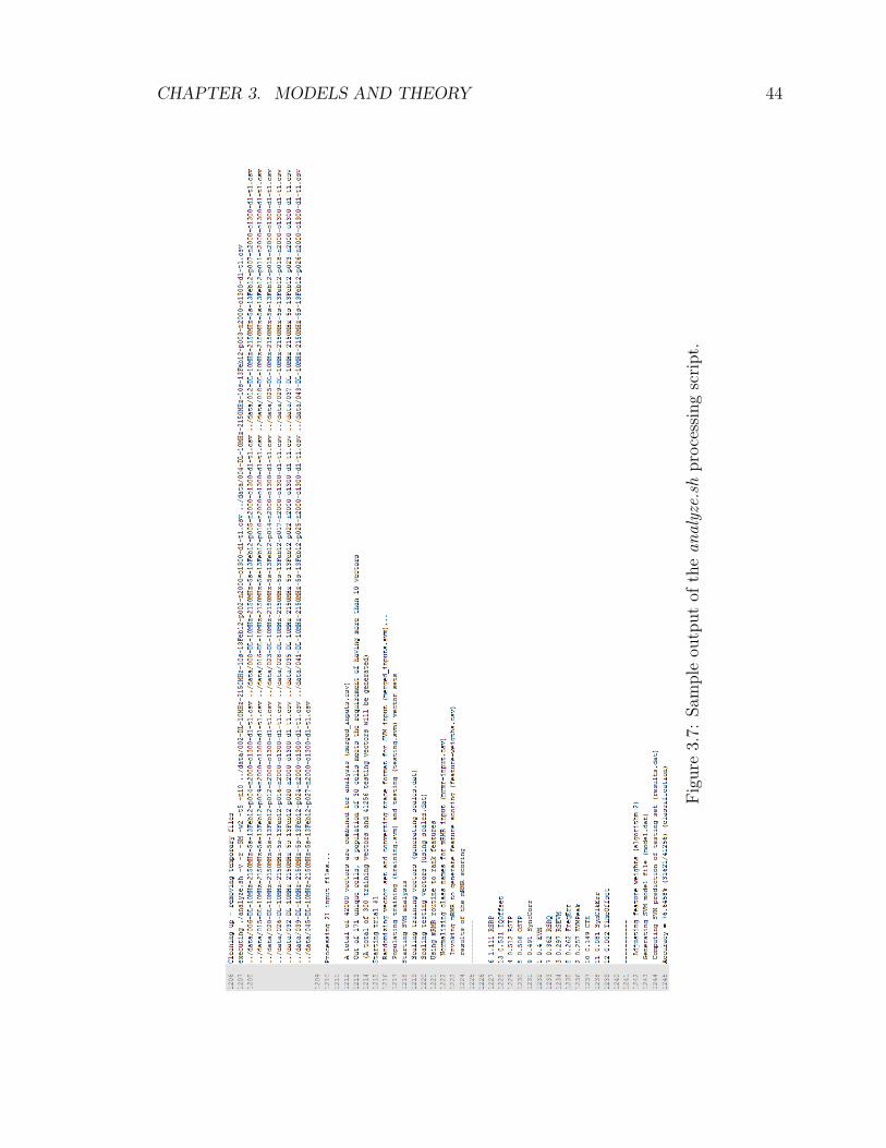
CHAPTER 3. MODELS AND THEORY 44
Figu
re3.7:
Sampleou
tput
ofthean
alyze.sh
processin
gscrip
t.
CHAPTER 3. MODELS AND THEORY 45
running log, and .pred gives testing result [41].
3.2.6 mrmr
Compiled version of the minimum-redundancy-maximum-relevance (mRMR) featureselection algorithm, provided by Peng et al. [44]. As the mrmr program requires adifferent trace format, analyze.sh first proceeds by reformatting the data. A discussionon mRMR is available in Subsection 3.4.2.
3.2.7 grid.py
The grid.py Python script is provided by the libsvm library as a tool to find theoptimal SVM parameters C and γ used with the RBF kernel function. It uses k-foldcross-validation and performs a grid search to determine the values of C and γ whichresult in the greatest prediction accuracy. Its usage is encouraged and explainedby Hsu et al. in [35]. A discussion on the requirement for this search appears inSection 3.6.
3.2.8 weight.awk
weight.awk is a simple awk script used to multiply the values of each feature using oneof five weighting algorithms. It uses, as input, the score or rank from either featurescoring algorithm. Weighting algorithms are discussed in detail in Section 3.5. Theoutput of the two scoring algorithms had to be standardized in order to be compatiblewith the weighting algorithms.
3.2.9 Computing Cell IDs
The statistics regarding the data collected during the Ottawa city field trial are com-piled in Table 4.1. The cell ID was computed using a concatenation of the CellId-GroupSector and the CellId fields from the trace extracts. Both of these entitiesare transmitted using a Zadoff-Chu sequence, in accordance with the LTE protocol.It was discovered that some cell IDs are used by both providers (both the CellId-GroupSector and CellId are identical). This explains why the number of cell IDswhen combining all recordings (3rd column) is less than the total number of cell IDsif treating the two providers independently (last column) in Table 4.1.
CHAPTER 3. MODELS AND THEORY 46
3.3 Signal Quality Filtering
A signal quality filter was programmed into the analysis tool in order to allow filter-ing of the vector set based on two binary signal quality parameters, namely signalsynchronization and decoded LTE frame number. Signal quality filtering was foundto greatly improve emitter re-identification success rates, while at the same time sig-nificantly reducing the pool of suitable parameter vectors for the SVM analysis (seeTable 4.1). Using command-line arguments during trace processing, it was possibleto exclude vectors that had one or two of the parameters unset.
3.3.1 Signal Synchronization
The program used to step through the RF recording and extract parameter vec-tors (VSA_Interface.xlsm) also retrieved and tabled two distinct values labelledas signal synchronization using the documented Agilent API. The AgtVsaVec-tor.Application.Measurement.Status was first recovered using the vsaStatusBitSync-NotFound bitmask (512) for every vector extracted, as well as the of the AgtVsaVec-tor.Application.Display.Traces(4).RawDataStatus (where 4 corresponds to the tracenumber for the D. Ch1 Error Summary Table) using the vsaTrcDatStaNoSync bit-mask (128). In practice, the data extracted showed that both signal synchroniza-tions were equal, and thus redundant, for all vectors extracted. Interestingly, AgilentTechnologies states in [42] that error measurements obtained in the absence of signalsynchronization are not considered for the averaging, when averaging is enabled inthe VSA software LTE demodulation properties. As such, it is recommended that atthe very least, only feature vectors extracted in the presence of signal synchroniza-tion be considered for further study. Chapter 4 results confirm that re-identificationresults are severely impacted when feature vectors extracted in the absence of signalsynchronization enter the SVM model, or are used as vectors under test.
3.3.2 Decoded Frame Number
In spite of the trace chosen for feature extraction, VSA_Interface.xlsm also capturedthe decoded downlink LTE frame number from the Ch1 DL Decode Info trace. Em-pirically, the decoded frame number was found to be a good indicator of receivedsignal quality, as recordings with marginal signal quality prevented the VSA softwarefrom properly decoding the LTE downlink frame number.
CHAPTER 3. MODELS AND THEORY 47
3.4 Feature Ranking and Scoring
When presented a large number of features, it is reasonable to assume not all featuresare as useful in identifying unknown classes. Some features may present little variationfrom class to class, whilst others may present little information that has not alreadybeen characterized by another feature. A common strategy in classification problemsis to make a determination which of the feature set should be emphasized, or evenwhich feature set could be safely ignored. In order to do so, one must first determine"which" features, and next determine how to conduct this emphasis. The approachselected for this research activity consisted in trialing two feature scoring algorithmsoften used in classification problems, which attempt to answer the first question:F-score and mRMR. Secondly, feature weighting was chosen as a method by whichemphasis could be applied, meaning most important features would be given a greaterweight prior to being modelled by the SVM classifier, after normalization. Weightingcan be seen as a more general case of feature exclusion, in which a set of n top featuresis kept whereas the others are discarded. In feature weighting, this is the equivalentof setting unselected features to a constant, nullifying their contribution to the SVMclassification model.
3.4.1 F-score
F-score is a simple technique which measures the discrimination of two sets of realnumbers. Given training vectors xk, k = 1, ...,m, if the number of positive andnegative instances are n+ and n−, respectively, then the F-score of the ith feature isdefined as:
F (i) ≡
(x
(+)i − xi
)2+(x
(−)i − xi
)2
1n+−1
n+∑k=1
(x
(+)k,i − x
(+)i
)2+ 1
n−−1
n−∑k=1
(x−k,i − x
(−)i
)2 (3.2)
where xi, x(+)i , and x
(−)i are the average of the feature of the whole, positive, and
negative data sets, respectively; x(+)k,i is the ith feature of the kth positive instance,
and x(−)k,i is the ith feature of the kth negative instance. The numerator indicates the
discrimination between the positive and negative sets, and the denominator indicatesthe one within each of the two sets. The larger the F-score is, the more likely thisfeature is more discriminative. A disadvantage of F-score is that is does not reveal
CHAPTER 3. MODELS AND THEORY 48
mutual information among features [47].
3.4.2 mRMR
One of the most popular approaches to realize Max-Dependency is maximal relevance(Max-Relevance) feature selection: selecting the features with the highest relevanceto the target class c. Relevance is usually characterized in terms of correlation ormutual information, of which the latter is one of the widely used measures to definedependency of variables [44]. In feature selection, it has been recognized that the com-binations of individually good features do not necessarily lead to good classificationperformance. In other words, "the m best features are not the best m features" [44].Some researchers have studied indirect or direct means to reduce the redundancyamong features and select features with the minimal redundancy (Min-Redundancy).The mRMR framework aims to minimize redundancy, used a series of intuitive mea-sures of relevance and redundancy to select promising features for both continuousand discrete data sets [44].
Max-Dependency has the following form:
maxD (S, c) , D = I (xi, i = 1, · · · ,M ; c) (3.3)
given the input data D tabled as N samples, andM features X = xi, i = 1, · · · ,M,and where I is the mutual information between variables, for a given class c. As Max-Dependency criterion is hard to implement, an alternative is to select features basedon maximal relevance criterion (Max-Relevance). Max-Relevance is to search fea-tures satisfying (3.4), which approximates D (S, c) with the mean value of all mutualinformation values between individual feature xi and class c, for a feature set S [44].
maxD (S, c) , D = 1|S|
∑I (xi; c) (3.4)
3.5 Feature Weighting and Selection
Once the features are ranked and scored by the scoring algorithm (either F-scoreor mRMR), it is possible to weight best features more heavily in an attempt toimprove SVM prediction accuracy. A number of algorithms are possible using eitherthe feature rank or feature score as input. The simplest approach is to multiply
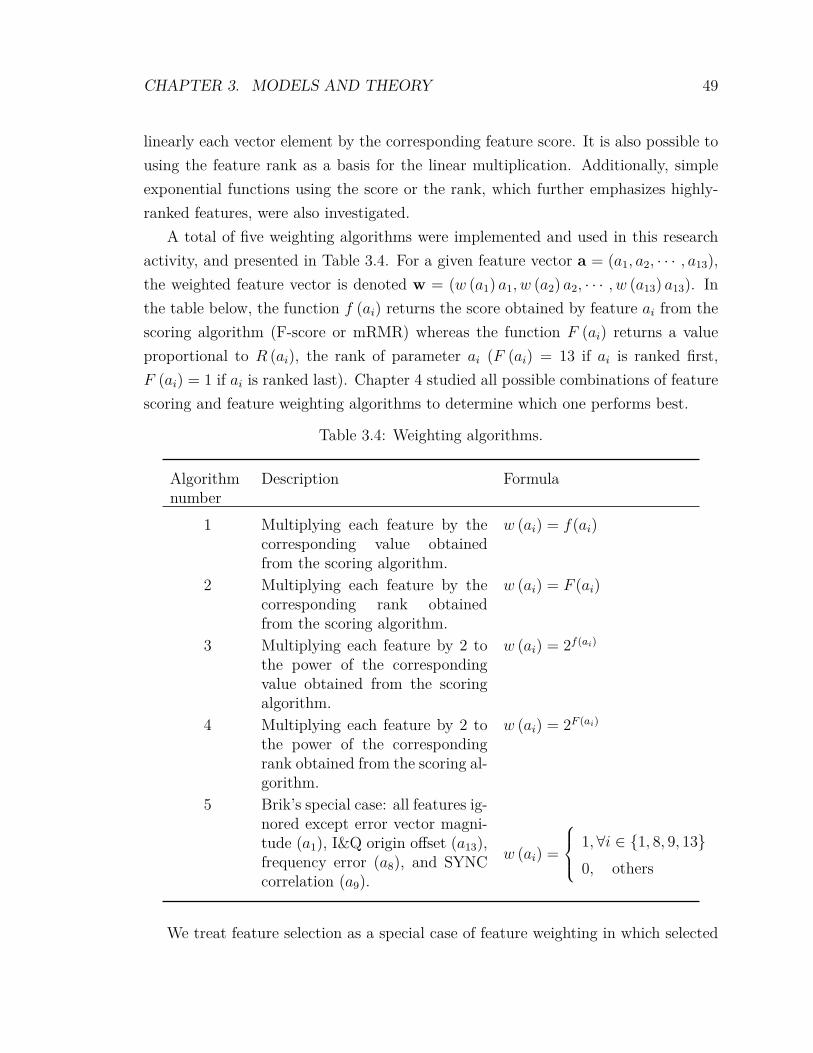
CHAPTER 3. MODELS AND THEORY 49
linearly each vector element by the corresponding feature score. It is also possible tousing the feature rank as a basis for the linear multiplication. Additionally, simpleexponential functions using the score or the rank, which further emphasizes highly-ranked features, were also investigated.
A total of five weighting algorithms were implemented and used in this researchactivity, and presented in Table 3.4. For a given feature vector a = (a1, a2, · · · , a13),the weighted feature vector is denoted w = (w (a1) a1, w (a2) a2, · · · , w (a13) a13). Inthe table below, the function f (ai) returns the score obtained by feature ai from thescoring algorithm (F-score or mRMR) whereas the function F (ai) returns a valueproportional to R (ai), the rank of parameter ai (F (ai) = 13 if ai is ranked first,F (ai) = 1 if ai is ranked last). Chapter 4 studied all possible combinations of featurescoring and feature weighting algorithms to determine which one performs best.
Table 3.4: Weighting algorithms.
Algorithmnumber
Description Formula
1 Multiplying each feature by thecorresponding value obtainedfrom the scoring algorithm.
w (ai) = f(ai)
2 Multiplying each feature by thecorresponding rank obtainedfrom the scoring algorithm.
w (ai) = F (ai)
3 Multiplying each feature by 2 tothe power of the correspondingvalue obtained from the scoringalgorithm.
w (ai) = 2f(ai)
4 Multiplying each feature by 2 tothe power of the correspondingrank obtained from the scoring al-gorithm.
w (ai) = 2F (ai)
5 Brik’s special case: all features ig-nored except error vector magni-tude (a1), I&Q origin offset (a13),frequency error (a8), and SYNCcorrelation (a9).
w (ai) =
1,∀i ∈ 1, 8, 9, 130, others
We treat feature selection as a special case of feature weighting in which selected
CHAPTER 3. MODELS AND THEORY 50
features are weighted with unity (i.e. retained) and all others ignored (zeroed). Themost useful application of feature selection is to retain only n features that are themost effective at re-identification, after scoring as in Equation (3.5). As an example,and in order to compare our results with the results obtained by Brik et al. in [2],we attempted to compute re-identification accuracy using the same five parameters,namely (from the most effective to the least effective) (i) frequency error, (ii) SYNCcorrelation, (iii) I&Q offset, (iv) magnitude error, and (v) phase error. However, thephase error was not available in the VSA trace used. Thus the Brik comparison ex-periments ignored all but four parameters, using the feature selection scheme outlinedin Table 3.4. Note that feature scoring was not required in the experiments using thefifth weighting algorithm, as it does not depend on either the score or the rank.
w (ai) =
1, ∀i ∈ R (ai) ≤ n
0, others(3.5)
3.6 SVM Parameters
Support vector machines attempt to find the solution to the optimization problemshown below
minw,b,ξ
12wTw + C
l∑i=1
ξi
subject to: yi(wTφ (xi) + b
)≥ 1− ξi, ξi ≥ 0 (3.6)
where C > 0 is the penalty parameter of the error term, also termed regularizationparameter. The kernel function K is defined in Equation (3.7), and is the functionused to express the hyperplane between classes. SVM, and libsvm in particular, offera number of choice of kernels functions: linear, polynomial of n degrees, RBF andsigmoid. The RBF kernel function is shown in Equation (3.8), where γ is the kernelparameter.

CHAPTER 3. MODELS AND THEORY 51
K (xi,xj) ≡ φ(xi)Tφ (xj) (3.7)K (xi,xj) = exp
(−γ‖xi − xj‖2
), γ > 0 (3.8)
There are two adjustable parameters when using an RBF kernel: C and γ. It isnot known beforehand which C and γ are best for a given problem; consequently somekind of model selection (parameter search) must be done. The goal is to identify goodparameters C and γ so that the classifier can accurately predict unknown data (i.e.testing data) [35]. The grid search method is recommended by Hsu in [35]. Variouspairs of C and γ values are tried and the one with the best cross-validation accuracyis picked. Hsu found that trying exponentially growing sequences of C and γ is apractical method to identify good parameters. In order to reduce the computationalrequirements, a coarse grid search first identifies a suitable regions, which is followedby a finer grid search within the suitable regions. libsvm provides a grid searchimplementation that can be used to find optimal C and γ for a given training set.
3.6.1 k-fold Cross-Validation
Prediction accuracy is often used as the optimization criteria for the C and γ kernelparameters. At its basis, the training dataset is randomly separated into two parts,of which one is considered unknown. The prediction accuracy obtained from the"unknown" set against the second part reflects the likely performance on classifyingan independent dataset. An improved version of this procedure is known as k-foldcross-validation. In k-fold cross-validation, the training dataset is first randomlydivided into k subsets of equal size. Sequentially, one subset is tested using theclassifier trained on the remaining k − 1 subsets. Thus, each instance of the wholetraining set is predicted once so the cross-validation accuracy is the percentage ofdata which is correctly classified. The cross-validation procedure can prevent theoverfitting problem [35].
3.7 Performance Evaluation
The SVM prediction accuracy, output by svm-predict was considered to be a relevantmeasure of re-identification accuracy. svm-predict is able to compare the predicted
CHAPTER 3. MODELS AND THEORY 52
class name with the actual class name which is also present in the dataset. It is alsopossible to conduct in-depth analysis looking into which cells are most often misiden-tified by the SVM model, or conversely which cells are most often incorrectly selectedby the SVM model. This knowledge could highlight the need to further discriminatebetween cells that have similar radiometric identities, using other methods. As thisin-depth analysis is only relevant to a specific data set and does not apply well toother experiments investigating different transmitters, it was deemed out of scope.Additional information concerning performance evaluation criteria is available in [2].
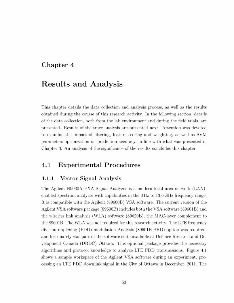
Chapter 4
Results and Analysis
This chapter details the data collection and analysis process, as well as the resultsobtained during the course of this research activity. In the following section, detailsof the data collection, both from the lab environment and during the field trials, arepresented. Results of the trace analysis are presented next. Attention was devotedto examine the impact of filtering, feature scoring and weighting, as well as SVMparameters optimization on prediction accuracy, in line with what was presented inChapter 3. An analysis of the significance of the results concludes this chapter.
4.1 Experimental Procedures
4.1.1 Vector Signal Analysis
The Agilent N9030A PXA Signal Analyzer is a modern local area network (LAN)-enabled spectrum analyzer with capabilities in the 3Hz to 13.6GHz frequency range.It is compatible with the Agilent (89600B) VSA software. The current version of theAgilent VSA software package (89600B) includes both the VSA software (89601B) andthe wireless link analysis (WLA) software (89620B), the MAC-layer complement tothe 89601B. The WLA was not required for this research activity. The LTE frequencydivision duplexing (FDD) modulation Analysis (89601B-BHD) option was required,and fortunately was part of the software suite available at Defence Research and De-velopment Canada (DRDC) Ottawa. This optional package provides the necessaryalgorithms and protocol knowledge to analyze LTE FDD transmissions. Figure 4.1shows a sample workspace of the Agilent VSA software during an experiment, pro-cessing an LTE FDD downlink signal in the City of Ottawa in December, 2011. The
53
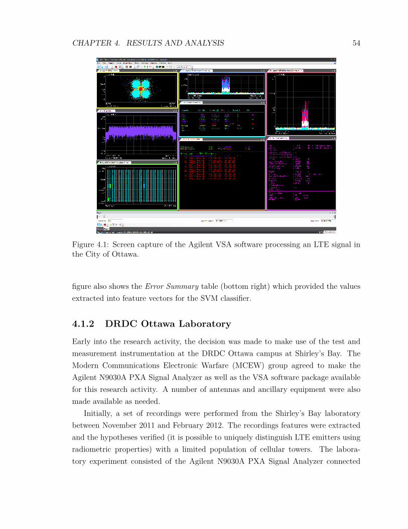
CHAPTER 4. RESULTS AND ANALYSIS 54
Figure 4.1: Screen capture of the Agilent VSA software processing an LTE signal inthe City of Ottawa.
figure also shows the Error Summary table (bottom right) which provided the valuesextracted into feature vectors for the SVM classifier.
4.1.2 DRDC Ottawa Laboratory
Early into the research activity, the decision was made to make use of the test andmeasurement instrumentation at the DRDC Ottawa campus at Shirley’s Bay. TheModern Communications Electronic Warfare (MCEW) group agreed to make theAgilent N9030A PXA Signal Analyzer as well as the VSA software package availablefor this research activity. A number of antennas and ancillary equipment were alsomade available as needed.
Initially, a set of recordings were performed from the Shirley’s Bay laboratorybetween November 2011 and February 2012. The recordings features were extractedand the hypotheses verified (it is possible to uniquely distinguish LTE emitters usingradiometric properties) with a limited population of cellular towers. The labora-tory experiment consisted of the Agilent N9030A PXA Signal Analyzer connected
CHAPTER 4. RESULTS AND ANALYSIS 55
Figure 4.2: Laboratory assembly.
to Kathrein 741790 omni-directional antenna installed on the roof of the building,through 22.9m of Times Microwave LMR-400 coaxial transmission line. The exter-nal 10MHz reference was provided by a Trimble Mini-T GPS Receiver board fed froma roof-mounted Trimble Bullet III GPS antenna (P/N 57860-00) through 22.9m ofBelden 1189A Dual Bond (R) IV 75 Ω. An HP Z400 workstation with Windows 7Professional (32 bits) ran the 32 bit version of the Agilent (89600B) VSA software(version 14.23). Figure 4.2 depicts the laboratory installation.
A total of 17 cells were observed from recordings at the Shirley’s Bay, between thetwo service providers who had active FDD LTE signals (Bell Canada and Rogers). Re-identification success rate peaked, after feature scoring and SVM kernel optimization,at 91%. However, the data collected during this phase did not include informationwhether the LTE downlink frame number was properly decoded or the VSA’s SYNCstatus. As discovered in subsequent experiments, having the ability to filter featurevectors based on signal quality improves the re-identification success rate.

CHAPTER 4. RESULTS AND ANALYSIS 56
Figure 4.3: Cellular tower locations in Ottawa, with data from [48].
4.1.3 Recordings from the City of Ottawa
Given the small population of cells within radio range to the Shirley’s Bay campus,the decision was made to perform recordings from various positions in the Ottawaarea. A route was planned around the City of Ottawa in order to increase the numberof candidate cells and determine if a larger population would harm re-identification.Route planning was conducted using cell tower positions available from [48]. Notethat [48] listed specific Rogers LTE tower positions but did not specify Bell LTE towerpositions. It was assumed, for the purpose of route planning, that Bell co-located LTEtowers with the HSPA towers. Tower positions around Ottawa for the two providersare amalgamated in Figure 4.3. The visualization service GPSvisualizer.com [45] wasused to generate the map, which was then modified using a text editor.
Since measurements would be taken only when the vehicle was at rest, the follow-ing factors were considered during route planning:
• Locations close to cell towers from two providers were favoured. This enabledmultiple recordings from a single position. The proximity to the towers alsoincreases the quality of the signal recording.
CHAPTER 4. RESULTS AND ANALYSIS 57
• A high concentration of towers were available in the down-town core. Thus asignificant number of the stops were planned within the down-town area.
• In order to test the effect of signal-to-noise ratio (SNR) on re-identificationsuccess rate, the route was planned to record signals from certain towers multipletimes, varying the distance to the towers.
Microsoft MapPoint with GPS dongle was used to confirm our position in relationto reported cell towers from [48]. A Garmin eTrex Vista HCx was used to record thegeographical coordinates of each recording position. The Agilent N9030A PXA SignalAnalyzer as well as the workstation with the VSA software package was removed fromthe laboratory and secured within a DRDC vehicle to perform the signal recordings.The PCTEL BLMPVDB700/2500 antenna with the BGMML195MSMA magneticbase was installed on top of the van and connected to the PXA using 3.6m of Pro-Flex Plus 195 coaxial cable. Again, the external 10MHz reference was provided by aTrimble Mini-T GPS Receiver board fed from a Trimble Bullet III GPS antenna P/N57860-00 through 22.9m of Belden 1189A Dual Bond (R) IV 75 Ω. The GPS antennaremained within the vehicle. A direct RJ-45 LAN connection was established betweenthe workstation and the PXA. Attempting to run the equipment using the on-boardalternator through an Absopulse sine-wave inverter resulted in abrupt power failuresat low engine revolutions per minute (RPM). This issue forced the research teamto stop and resume the experiment using a Honda 2 kW generator secured to a trayattached to the trailer-hitch. Figure 4.4 shows the experimental assembly for thisportion.
The recordings were conducted on February 13th, 2012. Both LTE cellularproviders in the area were active by that date. A total of 36 recording positionsgenerated 54 recordings, as both providers did not broadcast LTE signals from everyposition. The route followed, and each recording position, are overlaid on the towerpositions in Figure 4.5. A summary of the number of feature vectors extracted foreach provider is found in Table 4.1. For every recording, a set of 2000 feature vec-tors was extracted from the VSA software using VSA_Interface.xlsm. From the 2000vectors, a fraction had radio sync (94.6%) and a smaller fraction had both radio syncand a properly decoded frame number (30.8%).
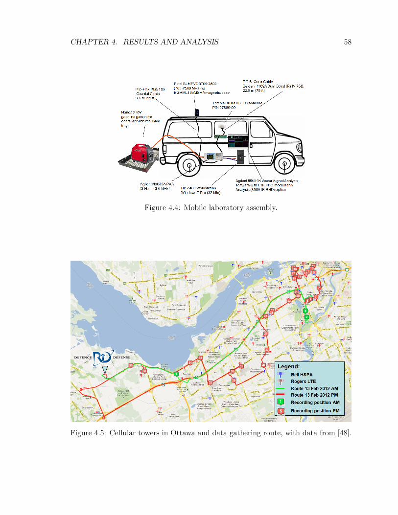
CHAPTER 4. RESULTS AND ANALYSIS 58
Figure 4.4: Mobile laboratory assembly.
Figure 4.5: Cellular towers in Ottawa and data gathering route, with data from [48].
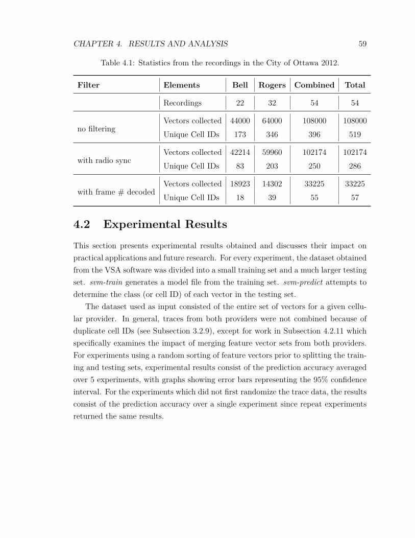
CHAPTER 4. RESULTS AND ANALYSIS 59
Table 4.1: Statistics from the recordings in the City of Ottawa 2012.
Filter Elements Bell Rogers Combined Total
Recordings 22 32 54 54
no filteringVectors collected 44000 64000 108000 108000Unique Cell IDs 173 346 396 519
with radio syncVectors collected 42214 59960 102174 102174Unique Cell IDs 83 203 250 286
with frame # decodedVectors collected 18923 14302 33225 33225Unique Cell IDs 18 39 55 57
4.2 Experimental Results
This section presents experimental results obtained and discusses their impact onpractical applications and future research. For every experiment, the dataset obtainedfrom the VSA software was divided into a small training set and a much larger testingset. svm-train generates a model file from the training set. svm-predict attempts todetermine the class (or cell ID) of each vector in the testing set.
The dataset used as input consisted of the entire set of vectors for a given cellu-lar provider. In general, traces from both providers were not combined because ofduplicate cell IDs (see Subsection 3.2.9), except for work in Subsection 4.2.11 whichspecifically examines the impact of merging feature vector sets from both providers.For experiments using a random sorting of feature vectors prior to splitting the train-ing and testing sets, experimental results consist of the prediction accuracy averagedover 5 experiments, with graphs showing error bars representing the 95% confidenceinterval. For the experiments which did not first randomize the trace data, the resultsconsist of the prediction accuracy over a single experiment since repeat experimentsreturned the same results.
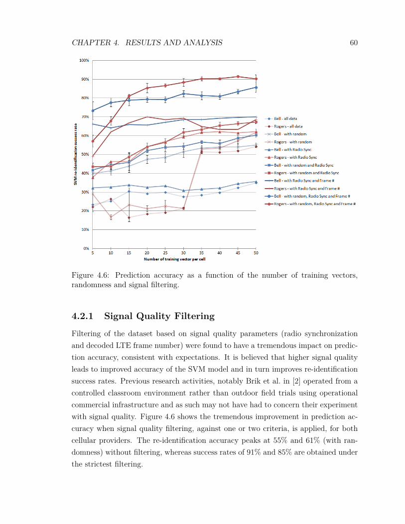
CHAPTER 4. RESULTS AND ANALYSIS 60
Figure 4.6: Prediction accuracy as a function of the number of training vectors,randomness and signal filtering.
4.2.1 Signal Quality Filtering
Filtering of the dataset based on signal quality parameters (radio synchronizationand decoded LTE frame number) were found to have a tremendous impact on predic-tion accuracy, consistent with expectations. It is believed that higher signal qualityleads to improved accuracy of the SVM model and in turn improves re-identificationsuccess rates. Previous research activities, notably Brik et al. in [2] operated from acontrolled classroom environment rather than outdoor field trials using operationalcommercial infrastructure and as such may not have had to concern their experimentwith signal quality. Figure 4.6 shows the tremendous improvement in prediction ac-curacy when signal quality filtering, against one or two criteria, is applied, for bothcellular providers. The re-identification accuracy peaks at 55% and 61% (with ran-domness) without filtering, whereas success rates of 91% and 85% are obtained underthe strictest filtering.
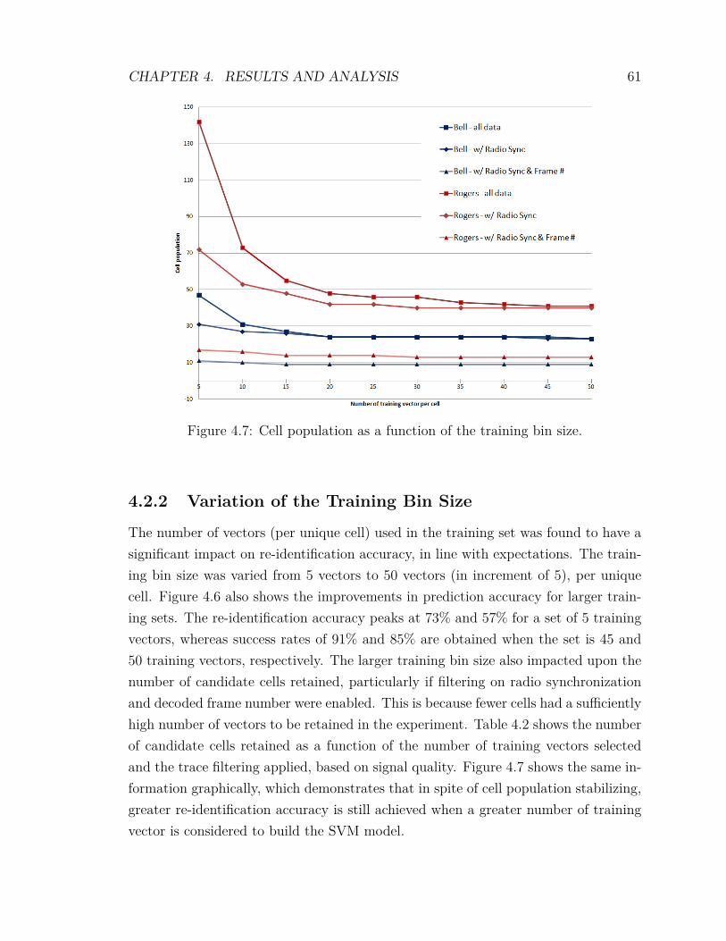
CHAPTER 4. RESULTS AND ANALYSIS 61
Figure 4.7: Cell population as a function of the training bin size.
4.2.2 Variation of the Training Bin Size
The number of vectors (per unique cell) used in the training set was found to have asignificant impact on re-identification accuracy, in line with expectations. The train-ing bin size was varied from 5 vectors to 50 vectors (in increment of 5), per uniquecell. Figure 4.6 also shows the improvements in prediction accuracy for larger train-ing sets. The re-identification accuracy peaks at 73% and 57% for a set of 5 trainingvectors, whereas success rates of 91% and 85% are obtained when the set is 45 and50 training vectors, respectively. The larger training bin size also impacted upon thenumber of candidate cells retained, particularly if filtering on radio synchronizationand decoded frame number were enabled. This is because fewer cells had a sufficientlyhigh number of vectors to be retained in the experiment. Table 4.2 shows the numberof candidate cells retained as a function of the number of training vectors selectedand the trace filtering applied, based on signal quality. Figure 4.7 shows the same in-formation graphically, which demonstrates that in spite of cell population stabilizing,greater re-identification accuracy is still achieved when a greater number of trainingvector is considered to build the SVM model.
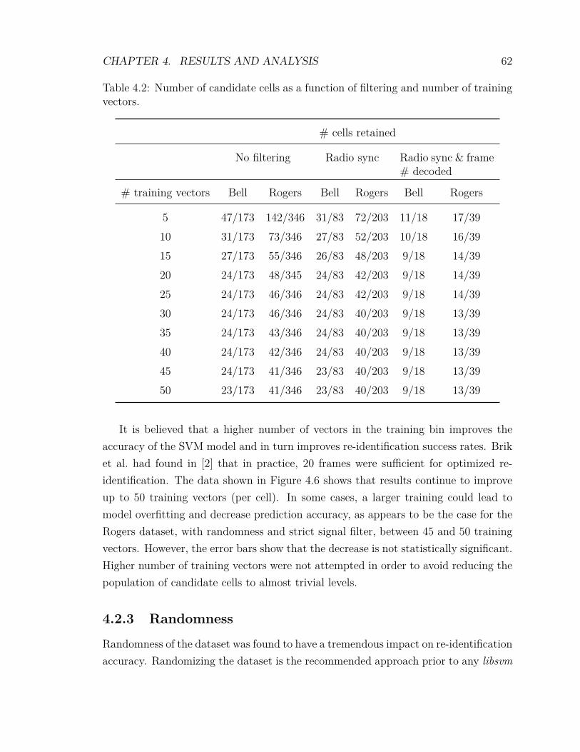
CHAPTER 4. RESULTS AND ANALYSIS 62
Table 4.2: Number of candidate cells as a function of filtering and number of trainingvectors.
# cells retained
No filtering Radio sync Radio sync & frame# decoded
# training vectors Bell Rogers Bell Rogers Bell Rogers
5 47/173 142/346 31/83 72/203 11/18 17/3910 31/173 73/346 27/83 52/203 10/18 16/3915 27/173 55/346 26/83 48/203 9/18 14/3920 24/173 48/345 24/83 42/203 9/18 14/3925 24/173 46/346 24/83 42/203 9/18 14/3930 24/173 46/346 24/83 40/203 9/18 13/3935 24/173 43/346 24/83 40/203 9/18 13/3940 24/173 42/346 24/83 40/203 9/18 13/3945 24/173 41/346 23/83 40/203 9/18 13/3950 23/173 41/346 23/83 40/203 9/18 13/39
It is believed that a higher number of vectors in the training bin improves theaccuracy of the SVM model and in turn improves re-identification success rates. Briket al. had found in [2] that in practice, 20 frames were sufficient for optimized re-identification. The data shown in Figure 4.6 shows that results continue to improveup to 50 training vectors (per cell). In some cases, a larger training could lead tomodel overfitting and decrease prediction accuracy, as appears to be the case for theRogers dataset, with randomness and strict signal filter, between 45 and 50 trainingvectors. However, the error bars show that the decrease is not statistically significant.Higher number of training vectors were not attempted in order to avoid reducing thepopulation of candidate cells to almost trivial levels.
4.2.3 Randomness
Randomness of the dataset was found to have a tremendous impact on re-identificationaccuracy. Randomizing the dataset is the recommended approach prior to any libsvm
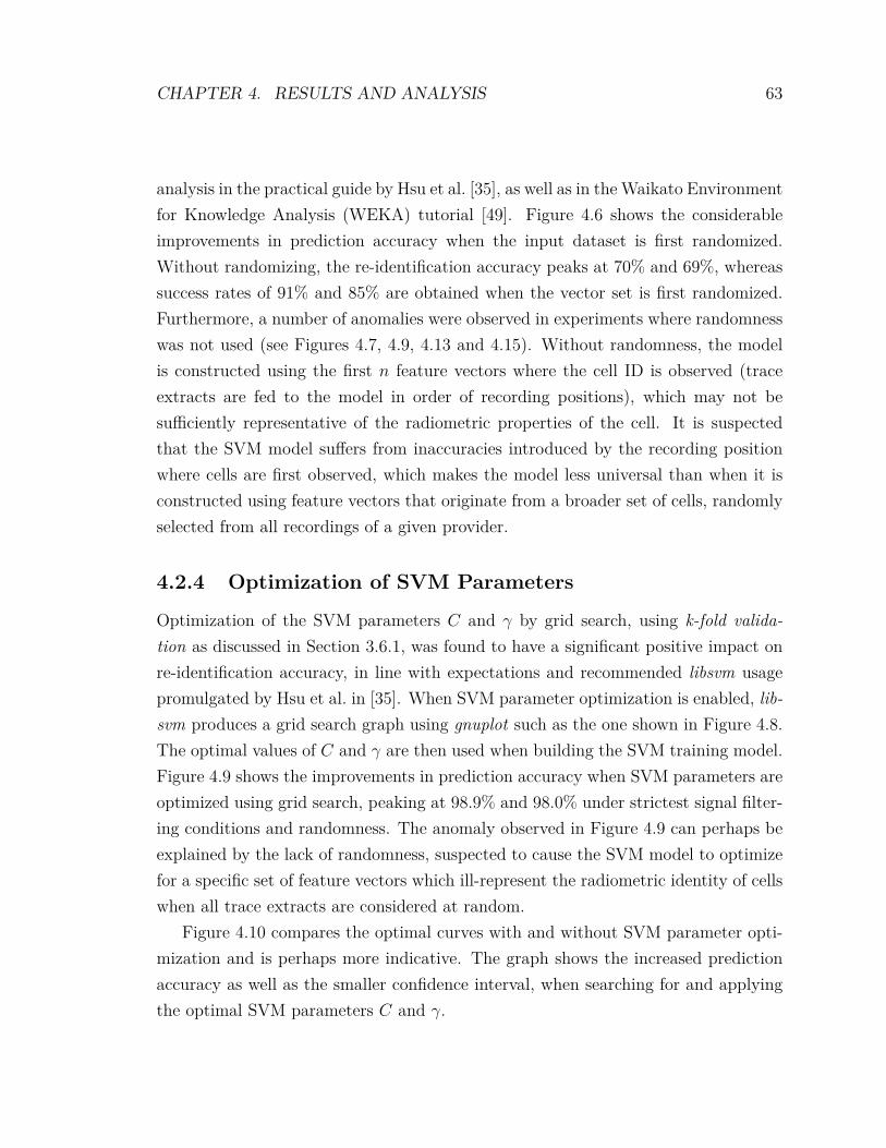
CHAPTER 4. RESULTS AND ANALYSIS 63
analysis in the practical guide by Hsu et al. [35], as well as in the Waikato Environmentfor Knowledge Analysis (WEKA) tutorial [49]. Figure 4.6 shows the considerableimprovements in prediction accuracy when the input dataset is first randomized.Without randomizing, the re-identification accuracy peaks at 70% and 69%, whereassuccess rates of 91% and 85% are obtained when the vector set is first randomized.Furthermore, a number of anomalies were observed in experiments where randomnesswas not used (see Figures 4.7, 4.9, 4.13 and 4.15). Without randomness, the modelis constructed using the first n feature vectors where the cell ID is observed (traceextracts are fed to the model in order of recording positions), which may not besufficiently representative of the radiometric properties of the cell. It is suspectedthat the SVM model suffers from inaccuracies introduced by the recording positionwhere cells are first observed, which makes the model less universal than when it isconstructed using feature vectors that originate from a broader set of cells, randomlyselected from all recordings of a given provider.
4.2.4 Optimization of SVM Parameters
Optimization of the SVM parameters C and γ by grid search, using k-fold valida-tion as discussed in Section 3.6.1, was found to have a significant positive impact onre-identification accuracy, in line with expectations and recommended libsvm usagepromulgated by Hsu et al. in [35]. When SVM parameter optimization is enabled, lib-svm produces a grid search graph using gnuplot such as the one shown in Figure 4.8.The optimal values of C and γ are then used when building the SVM training model.Figure 4.9 shows the improvements in prediction accuracy when SVM parameters areoptimized using grid search, peaking at 98.9% and 98.0% under strictest signal filter-ing conditions and randomness. The anomaly observed in Figure 4.9 can perhaps beexplained by the lack of randomness, suspected to cause the SVM model to optimizefor a specific set of feature vectors which ill-represent the radiometric identity of cellswhen all trace extracts are considered at random.
Figure 4.10 compares the optimal curves with and without SVM parameter opti-mization and is perhaps more indicative. The graph shows the increased predictionaccuracy as well as the smaller confidence interval, when searching for and applyingthe optimal SVM parameters C and γ.
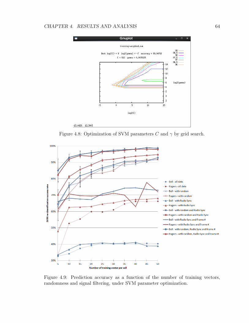
CHAPTER 4. RESULTS AND ANALYSIS 64
Figure 4.8: Optimization of SVM parameters C and γ by grid search.
Figure 4.9: Prediction accuracy as a function of the number of training vectors,randomness and signal filtering, under SVM parameter optimization.
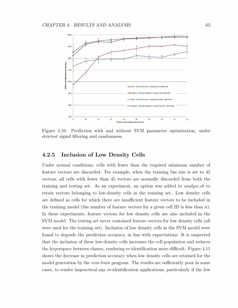
CHAPTER 4. RESULTS AND ANALYSIS 65
Figure 4.10: Prediction with and without SVM parameter optimization, understrictest signal filtering and randomness.
4.2.5 Inclusion of Low Density Cells
Under normal conditions, cells with fewer than the required minimum number offeature vectors are discarded. For example, when the training bin size is set to 45vectors, all cells with fewer than 45 vectors are normally discarded from both thetraining and testing set. As an experiment, an option was added to analyse.sh toretain vectors belonging to low-density cells in the training set. Low density cellsare defined as cells for which there are insufficient feature vectors to be included inthe training model (the number of feature vectors for a given cell ID is less than n).In these experiments, feature vectors for low density cells are also included in theSVM model. The testing set never contained feature vectors for low density cells (allwere used for the training set). Inclusion of low density cells in the SVM model werefound to degrade the prediction accuracy, in line with expectations. It is suspectedthat the inclusion of these low-density cells increases the cell population and reducesthe hyperspace between classes, rendering re-identification more difficult. Figure 4.11shows the decrease in prediction accuracy when low density cells are retained for themodel generation by the svm-train program. The results are sufficiently poor in somecases, to render impractical any re-identification applications, particularly if the low
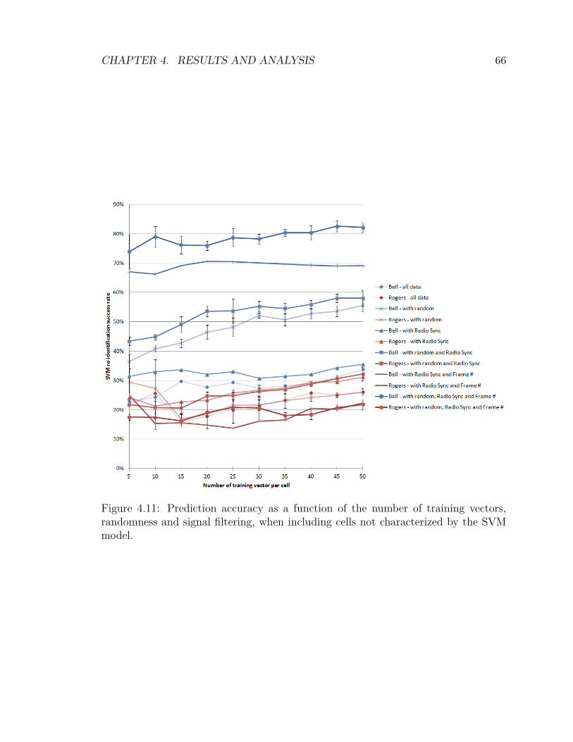
CHAPTER 4. RESULTS AND ANALYSIS 66
Figure 4.11: Prediction accuracy as a function of the number of training vectors,randomness and signal filtering, when including cells not characterized by the SVMmodel.
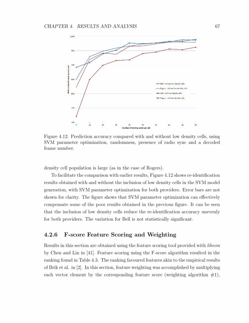
CHAPTER 4. RESULTS AND ANALYSIS 67
Figure 4.12: Prediction accuracy compared with and without low density cells, usingSVM parameter optimization, randomness, presence of radio sync and a decodedframe number.
density cell population is large (as in the case of Rogers).To facilitate the comparison with earlier results, Figure 4.12 shows re-identification
results obtained with and without the inclusion of low density cells in the SVM modelgeneration, with SVM parameter optimization for both providers. Error bars are notshown for clarity. The figure shows that SVM parameter optimization can effectivelycompensate some of the poor results obtained in the previous figure. It can be seenthat the inclusion of low density cells reduce the re-identification accuracy unevenlyfor both providers. The variation for Bell is not statistically significant.
4.2.6 F-score Feature Scoring and Weighting
Results in this section are obtained using the feature scoring tool provided with libsvmby Chen and Lin in [41]. Feature scoring using the F-score algorithm resulted in theranking found in Table 4.3. The ranking favoured features akin to the empirical resultsof Brik et al. in [2]. In this section, feature weighting was accomplished by multiplyingeach vector element by the corresponding feature score (weighting algorithm #1),
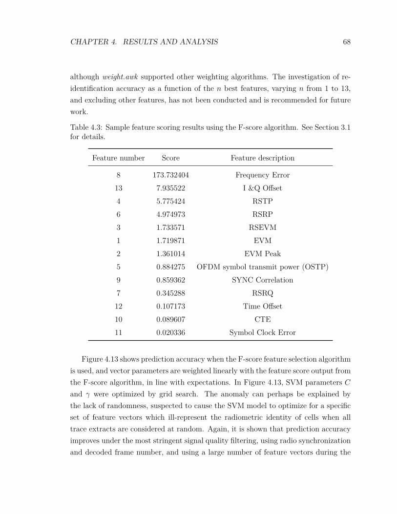
CHAPTER 4. RESULTS AND ANALYSIS 68
although weight.awk supported other weighting algorithms. The investigation of re-identification accuracy as a function of the n best features, varying n from 1 to 13,and excluding other features, has not been conducted and is recommended for futurework.
Table 4.3: Sample feature scoring results using the F-score algorithm. See Section 3.1for details.
Feature number Score Feature description
8 173.732404 Frequency Error13 7.935522 I &Q Offset4 5.775424 RSTP6 4.974973 RSRP3 1.733571 RSEVM1 1.719871 EVM2 1.361014 EVM Peak5 0.884275 OFDM symbol transmit power (OSTP)9 0.859362 SYNC Correlation7 0.345288 RSRQ12 0.107173 Time Offset10 0.089607 CTE11 0.020336 Symbol Clock Error
Figure 4.13 shows prediction accuracy when the F-score feature selection algorithmis used, and vector parameters are weighted linearly with the feature score output fromthe F-score algorithm, in line with expectations. In Figure 4.13, SVM parameters Cand γ were optimized by grid search. The anomaly can perhaps be explained bythe lack of randomness, suspected to cause the SVM model to optimize for a specificset of feature vectors which ill-represent the radiometric identity of cells when alltrace extracts are considered at random. Again, it is shown that prediction accuracyimproves under the most stringent signal quality filtering, using radio synchronizationand decoded frame number, and using a large number of feature vectors during the
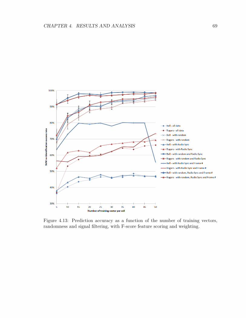
CHAPTER 4. RESULTS AND ANALYSIS 69
Figure 4.13: Prediction accuracy as a function of the number of training vectors,randomness and signal filtering, with F-score feature scoring and weighting.
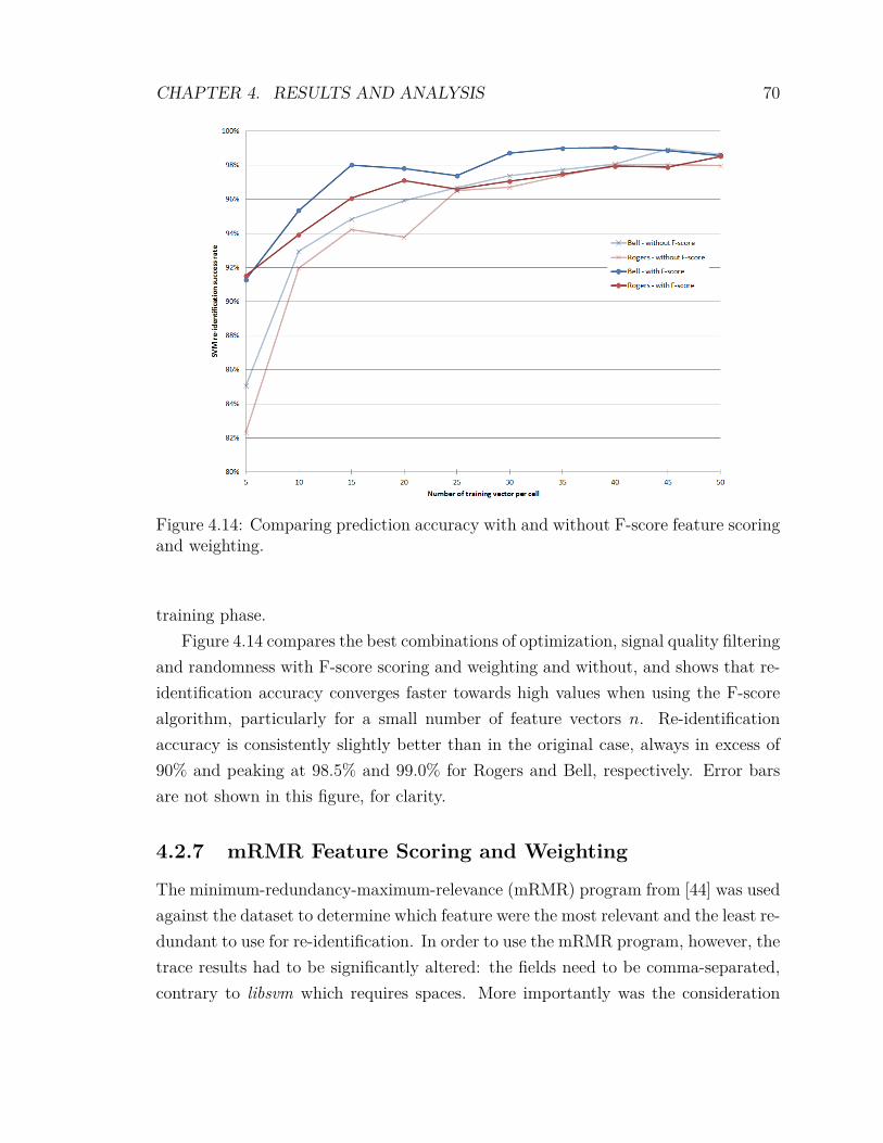
CHAPTER 4. RESULTS AND ANALYSIS 70
Figure 4.14: Comparing prediction accuracy with and without F-score feature scoringand weighting.
training phase.Figure 4.14 compares the best combinations of optimization, signal quality filtering
and randomness with F-score scoring and weighting and without, and shows that re-identification accuracy converges faster towards high values when using the F-scorealgorithm, particularly for a small number of feature vectors n. Re-identificationaccuracy is consistently slightly better than in the original case, always in excess of90% and peaking at 98.5% and 99.0% for Rogers and Bell, respectively. Error barsare not shown in this figure, for clarity.
4.2.7 mRMR Feature Scoring and Weighting
The minimum-redundancy-maximum-relevance (mRMR) program from [44] was usedagainst the dataset to determine which feature were the most relevant and the least re-dundant to use for re-identification. In order to use the mRMR program, however, thetrace results had to be significantly altered: the fields need to be comma-separated,contrary to libsvm which requires spaces. More importantly was the consideration
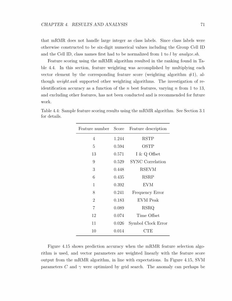
CHAPTER 4. RESULTS AND ANALYSIS 71
that mRMR does not handle large integer as class labels. Since class labels wereotherwise constructed to be six-digit numerical values including the Group Cell IDand the Cell ID, class names first had to be normalized from 1 to l by analyze.sh.
Feature scoring using the mRMR algorithm resulted in the ranking found in Ta-ble 4.4. In this section, feature weighting was accomplished by multiplying eachvector element by the corresponding feature score (weighting algorithm #1), al-though weight.awk supported other weighting algorithms. The investigation of re-identification accuracy as a function of the n best features, varying n from 1 to 13,and excluding other features, has not been conducted and is recommended for futurework.
Table 4.4: Sample feature scoring results using the mRMR algorithm. See Section 3.1for details.
Feature number Score Feature description
4 1.244 RSTP5 0.594 OSTP13 0.571 I & Q Offset9 0.529 SYNC Correlation3 0.448 RSEVM6 0.435 RSRP1 0.392 EVM8 0.241 Frequency Error2 0.183 EVM Peak7 0.089 RSRQ12 0.074 Time Offset11 0.026 Symbol Clock Error10 0.014 CTE
Figure 4.15 shows prediction accuracy when the mRMR feature selection algo-rithm is used, and vector parameters are weighted linearly with the feature scoreoutput from the mRMR algorithm, in line with expectations. In Figure 4.15, SVMparameters C and γ were optimized by grid search. The anomaly can perhaps be
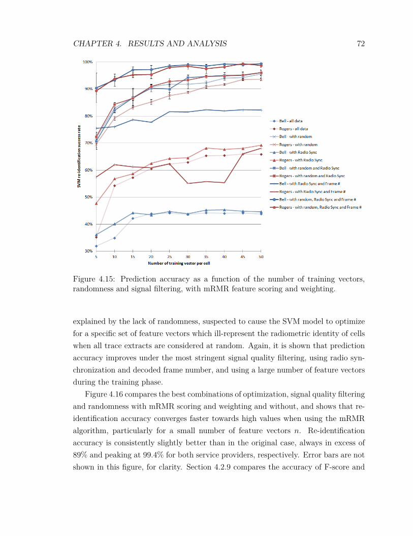
CHAPTER 4. RESULTS AND ANALYSIS 72
Figure 4.15: Prediction accuracy as a function of the number of training vectors,randomness and signal filtering, with mRMR feature scoring and weighting.
explained by the lack of randomness, suspected to cause the SVM model to optimizefor a specific set of feature vectors which ill-represent the radiometric identity of cellswhen all trace extracts are considered at random. Again, it is shown that predictionaccuracy improves under the most stringent signal quality filtering, using radio syn-chronization and decoded frame number, and using a large number of feature vectorsduring the training phase.
Figure 4.16 compares the best combinations of optimization, signal quality filteringand randomness with mRMR scoring and weighting and without, and shows that re-identification accuracy converges faster towards high values when using the mRMRalgorithm, particularly for a small number of feature vectors n. Re-identificationaccuracy is consistently slightly better than in the original case, always in excess of89% and peaking at 99.4% for both service providers, respectively. Error bars are notshown in this figure, for clarity. Section 4.2.9 compares the accuracy of F-score and
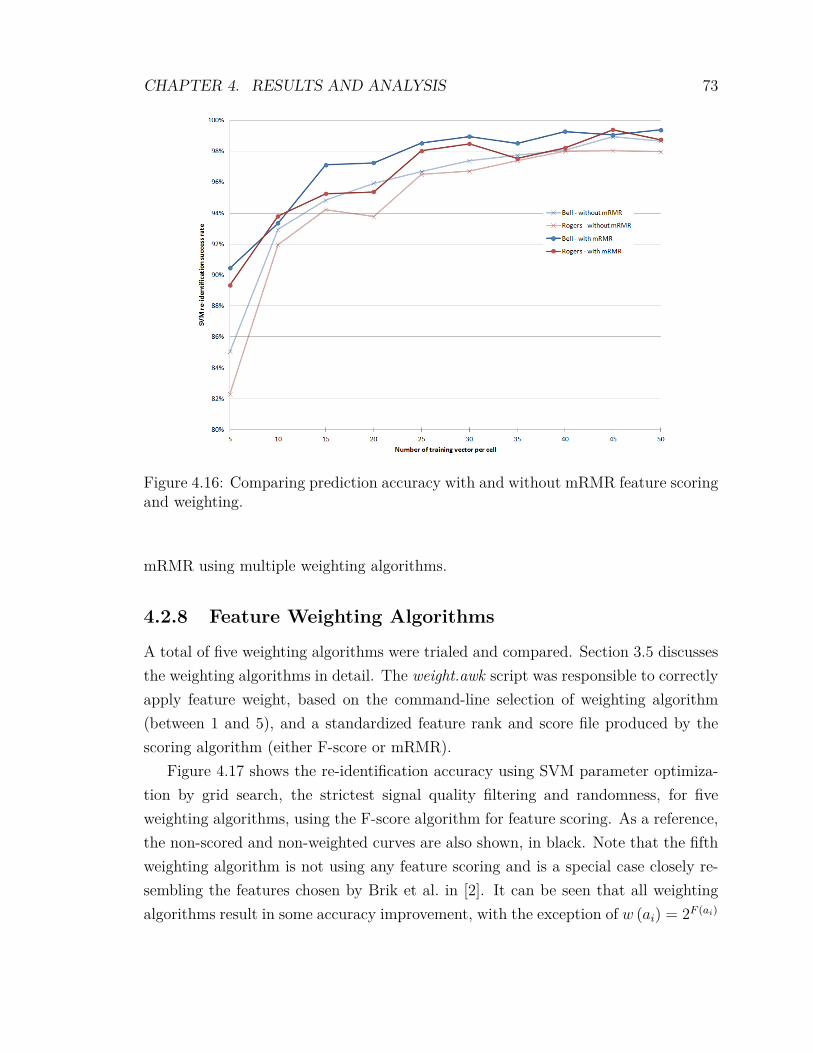
CHAPTER 4. RESULTS AND ANALYSIS 73
Figure 4.16: Comparing prediction accuracy with and without mRMR feature scoringand weighting.
mRMR using multiple weighting algorithms.
4.2.8 Feature Weighting Algorithms
A total of five weighting algorithms were trialed and compared. Section 3.5 discussesthe weighting algorithms in detail. The weight.awk script was responsible to correctlyapply feature weight, based on the command-line selection of weighting algorithm(between 1 and 5), and a standardized feature rank and score file produced by thescoring algorithm (either F-score or mRMR).
Figure 4.17 shows the re-identification accuracy using SVM parameter optimiza-tion by grid search, the strictest signal quality filtering and randomness, for fiveweighting algorithms, using the F-score algorithm for feature scoring. As a reference,the non-scored and non-weighted curves are also shown, in black. Note that the fifthweighting algorithm is not using any feature scoring and is a special case closely re-sembling the features chosen by Brik et al. in [2]. It can be seen that all weightingalgorithms result in some accuracy improvement, with the exception of w (ai) = 2F (ai)
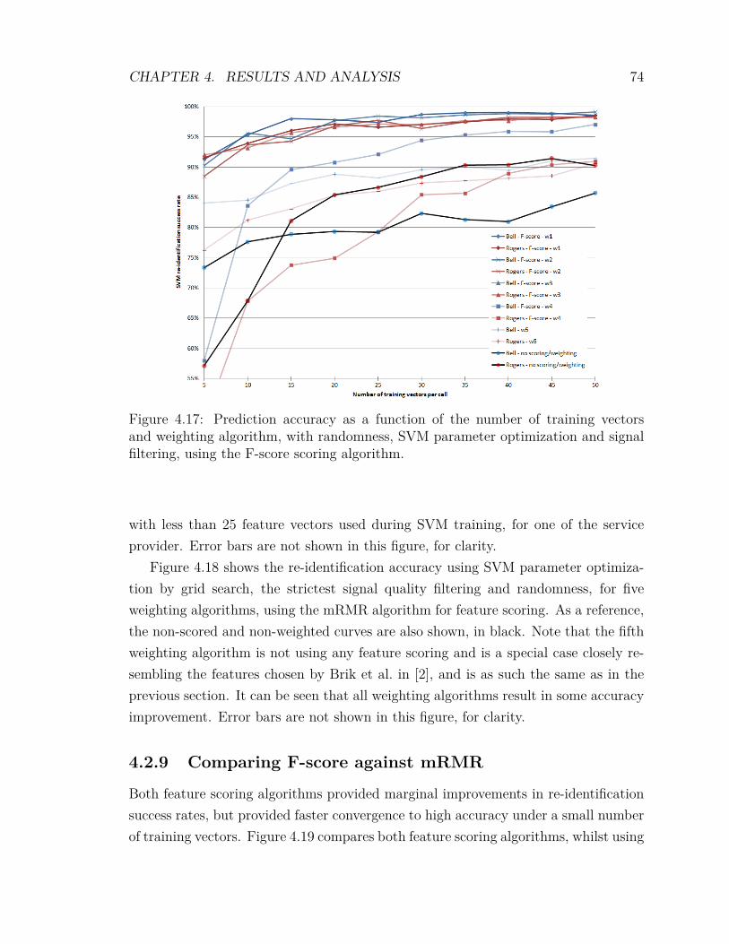
CHAPTER 4. RESULTS AND ANALYSIS 74
Figure 4.17: Prediction accuracy as a function of the number of training vectorsand weighting algorithm, with randomness, SVM parameter optimization and signalfiltering, using the F-score scoring algorithm.
with less than 25 feature vectors used during SVM training, for one of the serviceprovider. Error bars are not shown in this figure, for clarity.
Figure 4.18 shows the re-identification accuracy using SVM parameter optimiza-tion by grid search, the strictest signal quality filtering and randomness, for fiveweighting algorithms, using the mRMR algorithm for feature scoring. As a reference,the non-scored and non-weighted curves are also shown, in black. Note that the fifthweighting algorithm is not using any feature scoring and is a special case closely re-sembling the features chosen by Brik et al. in [2], and is as such the same as in theprevious section. It can be seen that all weighting algorithms result in some accuracyimprovement. Error bars are not shown in this figure, for clarity.
4.2.9 Comparing F-score against mRMR
Both feature scoring algorithms provided marginal improvements in re-identificationsuccess rates, but provided faster convergence to high accuracy under a small numberof training vectors. Figure 4.19 compares both feature scoring algorithms, whilst using
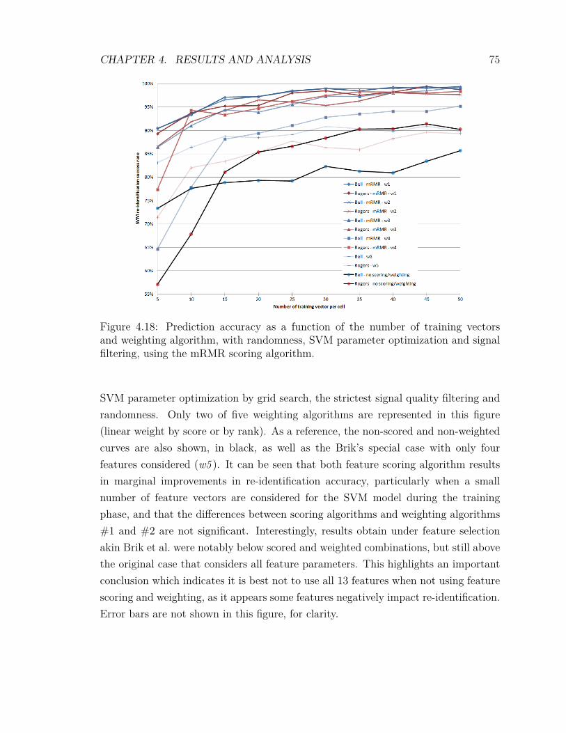
CHAPTER 4. RESULTS AND ANALYSIS 75
Figure 4.18: Prediction accuracy as a function of the number of training vectorsand weighting algorithm, with randomness, SVM parameter optimization and signalfiltering, using the mRMR scoring algorithm.
SVM parameter optimization by grid search, the strictest signal quality filtering andrandomness. Only two of five weighting algorithms are represented in this figure(linear weight by score or by rank). As a reference, the non-scored and non-weightedcurves are also shown, in black, as well as the Brik’s special case with only fourfeatures considered (w5 ). It can be seen that both feature scoring algorithm resultsin marginal improvements in re-identification accuracy, particularly when a smallnumber of feature vectors are considered for the SVM model during the trainingphase, and that the differences between scoring algorithms and weighting algorithms#1 and #2 are not significant. Interestingly, results obtain under feature selectionakin Brik et al. were notably below scored and weighted combinations, but still abovethe original case that considers all feature parameters. This highlights an importantconclusion which indicates it is best not to use all 13 features when not using featurescoring and weighting, as it appears some features negatively impact re-identification.Error bars are not shown in this figure, for clarity.
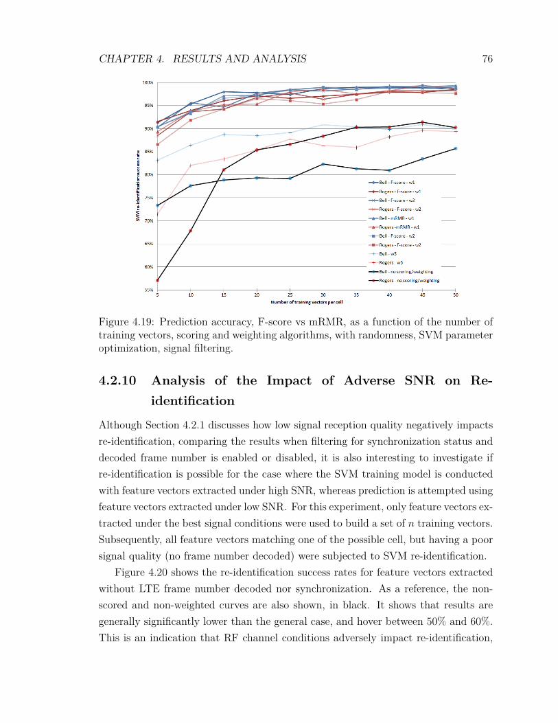
CHAPTER 4. RESULTS AND ANALYSIS 76
Figure 4.19: Prediction accuracy, F-score vs mRMR, as a function of the number oftraining vectors, scoring and weighting algorithms, with randomness, SVM parameteroptimization, signal filtering.
4.2.10 Analysis of the Impact of Adverse SNR on Re-identification
Although Section 4.2.1 discusses how low signal reception quality negatively impactsre-identification, comparing the results when filtering for synchronization status anddecoded frame number is enabled or disabled, it is also interesting to investigate ifre-identification is possible for the case where the SVM training model is conductedwith feature vectors extracted under high SNR, whereas prediction is attempted usingfeature vectors extracted under low SNR. For this experiment, only feature vectors ex-tracted under the best signal conditions were used to build a set of n training vectors.Subsequently, all feature vectors matching one of the possible cell, but having a poorsignal quality (no frame number decoded) were subjected to SVM re-identification.
Figure 4.20 shows the re-identification success rates for feature vectors extractedwithout LTE frame number decoded nor synchronization. As a reference, the non-scored and non-weighted curves are also shown, in black. It shows that results aregenerally significantly lower than the general case, and hover between 50% and 60%.This is an indication that RF channel conditions adversely impact re-identification,
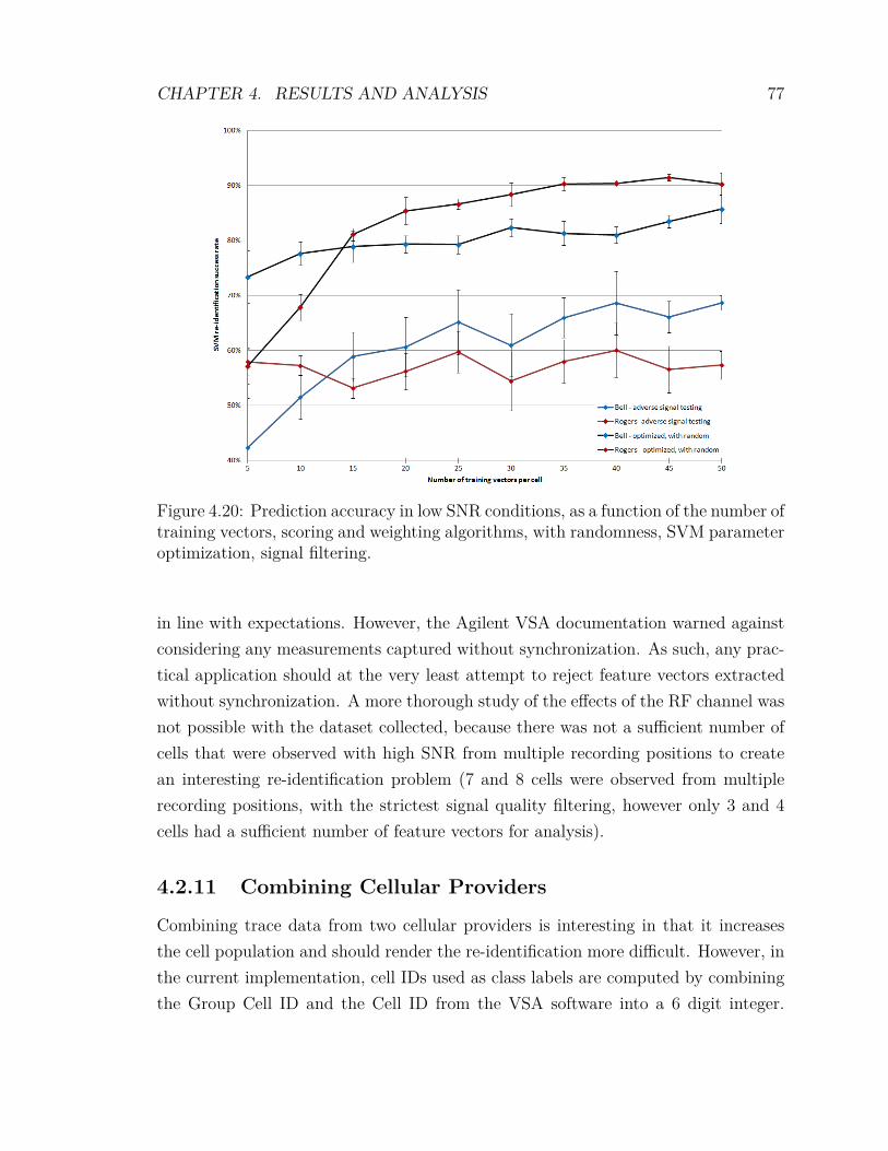
CHAPTER 4. RESULTS AND ANALYSIS 77
Figure 4.20: Prediction accuracy in low SNR conditions, as a function of the number oftraining vectors, scoring and weighting algorithms, with randomness, SVM parameteroptimization, signal filtering.
in line with expectations. However, the Agilent VSA documentation warned againstconsidering any measurements captured without synchronization. As such, any prac-tical application should at the very least attempt to reject feature vectors extractedwithout synchronization. A more thorough study of the effects of the RF channel wasnot possible with the dataset collected, because there was not a sufficient number ofcells that were observed with high SNR from multiple recording positions to createan interesting re-identification problem (7 and 8 cells were observed from multiplerecording positions, with the strictest signal quality filtering, however only 3 and 4cells had a sufficient number of feature vectors for analysis).
4.2.11 Combining Cellular Providers
Combining trace data from two cellular providers is interesting in that it increasesthe cell population and should render the re-identification more difficult. However, inthe current implementation, cell IDs used as class labels are computed by combiningthe Group Cell ID and the Cell ID from the VSA software into a 6 digit integer.
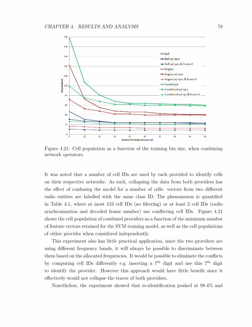
CHAPTER 4. RESULTS AND ANALYSIS 78
Figure 4.21: Cell population as a function of the training bin size, when combiningnetwork operators.
It was noted that a number of cell IDs are used by each provided to identify cellson their respective networks. As such, collapsing the data from both providers hasthe effect of confusing the model for a number of cells: vectors from two differentradio entities are labelled with the same class ID. The phenomenon is quantifiedin Table 4.1, where at most 123 cell IDs (no filtering) or at least 2 cell IDs (radiosynchronization and decoded frame number) use conflicting cell IDs. Figure 4.21shows the cell population of combined providers as a function of the minimum numberof feature vectors retained for the SVM training model, as well as the cell populationsof either provider when considered independently.
This experiment also has little practical application, since the two providers areusing different frequency bands, it will always be possible to discriminate betweenthem based on the allocated frequencies. It would be possible to eliminate the conflictsby computing cell IDs differently e.g. inserting a 7th digit and use this 7th digitto identify the provider. However this approach would have little benefit since iteffectively would not collapse the traces of both providers.
Nonetheless, the experiment showed that re-identification peaked at 98.4% and
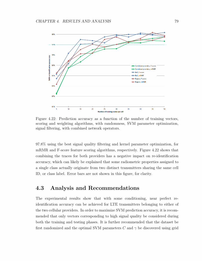
CHAPTER 4. RESULTS AND ANALYSIS 79
Figure 4.22: Prediction accuracy as a function of the number of training vectors,scoring and weighting algorithms, with randomness, SVM parameter optimization,signal filtering, with combined network operators.
97.8% using the best signal quality filtering and kernel parameter optimization, formRMR and F-score feature scoring algorithms, respectively. Figure 4.22 shows thatcombining the traces for both providers has a negative impact on re-identificationaccuracy, which can likely be explained that some radiometric properties assigned toa single class actually originate from two distinct transmitters sharing the same cellID, or class label. Error bars are not shown in this figure, for clarity.
4.3 Analysis and Recommendations
The experimental results show that with some conditioning, near perfect re-identification accuracy can be achieved for LTE transmitters belonging to either ofthe two cellular providers. In order to maximize SVM prediction accuracy, it is recom-mended that only vectors corresponding to high signal quality be considered duringboth the training and testing phases. It is further recommended that the dataset befirst randomized and the optimal SVM parameters C and γ be discovered using grid
CHAPTER 4. RESULTS AND ANALYSIS 80
search, both recommended by Hsu in [35]. The use of feature scoring and weight-ing always resulted in faster convergence with a small number of training vectorsand results in non-negligible improvements in re-identification accuracy. The choiceof the weighting algorithm or the feature scoring algorithm did not however resultin significant variations, indicating that as long as key features are given more im-portance, improvements are obtained, regardless of the relative importance betweenfeatures. Both feature scoring algorithms were found to score features in a compara-ble order, even though they operated fundamentally differently, in that mRMR alsoattempted to reduce redundancy between features; three out of the top five featureswere common between the two scoring algorithms. Interestingly, a feature selectionof the four features closest to the Brik et al. experiments in [2] also resulted in im-provements over the general non-optimized case, indicating that some of the featuresare detrimental to re-identification when considered in the SVM training model, par-ticularly when the SVM parameters are not optimized by grid search. Lastly, theprediction accuracy was shown to improve when a larger set of feature vectors aresupplied to build the SVM training model (best results consistently obtained with 45to 50 training vectors); however, when feature scoring and weighting is applied, andoptimal C and γ are discovered, results well above 90% are obtained with as few as10 training vectors. Larger sets of training vector in those experiments only result inmarginal accuracy gains. It should be noted that in this thesis, the re-identificationof each unknown emitters was conducted using a single feature vector (i.e. a testingbin size of 1), leading to great results. In practical applications, it may be possibleto gather several feature vectors from an unknown transmitter in order to determineits identity, which is expected to result in even greater accuracy.
Chapter 5
Conclusions and Future Work
LTE is an emerging communication standard already available in many urban centresworldwide. Competing 4G cellular technologies have been abandoned by standardbodies (e.g. UMB) or by the majority of network operators (e.g. WiMAX), open-ing the door for a first truly global cellular standard. This research demonstratedthat sufficient differences exist between LTE transmitters to enable near-perfect re-identification, for both service providers, based on radiometric properties of the down-link signal.
This chapter first reviews the results achieved, in line with the contributions listedin Chapter 1. Potential applications of these excellent results in solving practicalproblems are also proposed. Next, limitations observed during this research are high-lighted, followed by several recommendations for further research, building upon theresults shown herein.
5.1 Contributions, Results and Applications
This section first reviews the research objectives considered at the onset of this study,and presents a brief overview of the results achieved. Practical applications that coulduse radiometric identifications are then presented.
5.1.1 Main Contributions and Results Overview
This research activity attempted to and succeeded in presenting novel contributionsin the following areas:
• First successful radiometric identification of LTE transmitters. Re-identification
81
CHAPTER 5. CONCLUSIONS AND FUTURE WORK 82
of LTE downlink transmitters was shown to be possible with an accuracy inexcess of 99%, using commercially-available hardware and software, combinedwith an established classifier algorithm (SVM).
• First successful use of a weighted classifier algorithm (weighted-SVM) to con-duct radiometric identification. This thesis showed that feature scoring andweighting had a beneficial impact on re-identification due to faster conver-gence towards accurate prediction with fewer training vectors. The F-scoreand mRMR scoring algorithms scored features in a comparable fashion, as ex-pected. Four weighting algorithms (linear by score or rank, exponential by scoreor rank) were trialed for both F-score and mRMR scoring, as well as a specialcase of feature selection using only four features. All weighting algorithms re-sulted in similar improvements, whereas the feature selection trial exhibitedlower improvement but still outperformed the general non-optimized case.
• First examination of the impact of variable modulation schemes on radiometricidentification. This thesis demonstrated that radiometric identification was suc-cessful in spite of the LTE downlink supporting multiple modulation schemes. Itis not certain, however, that all modulation schemes were present in the record-ings analyzed by the VSA software, because the Error Summary table did notspecifically provide error summary values for each of the modulation observedin the downlink, against expectations (see Figure 3.4). It is believed that thevarious modulation schemes observed on the different downlink channels wereaggregated in a single set of error values and this was shown not impede accuratere-identification.
5.1.2 Applications
Enhancement to Identity Verification and Authentication
The LTE standard has been designed from the ground up with security and privacyin mind. As such, there are a number of measures and techniques already in place toprotect the identity of users, and ensure communication and location privacy.
Radiometric identification can be considered as a complement to existing crypto-graphic techniques and should be fairly easy to implement. Radio receiving equipmentis already capable of performing some analysis of the modulation characteristics of
CHAPTER 5. CONCLUSIONS AND FUTURE WORK 83
nearby emitters, providing network operators the ability to black-list handsets whichfail to comply to communication standards. Based on the results of this research,it should be possible to validate the identity of a base station using its radiometricproperties, in order to detect man-in-the-middle attacks or spoofing that might havegone undetected otherwise. Expensive and highly sensitive spectrum analysis equip-ment such as the one used for this thesis may not be required, as demonstrated bywork by Edman and Yener in [33] showing re-identification success rates of 87% usinginexpensive equipment such as the USRP. It is believe that radiometric identifica-tion opportunities using band-optimized radio electronics present in modern phonesis conceivable in the near future.
In a conceptual system, network operators could be responsible to maintain a validclassifier model which describes the equipment they legitimately field. This could bedone by the network operator or crowd-sourced by users running a trusted applicationwhich would submit feature vectors over time. During testing, the UE could querythe provider with a test feature vector, or could run the classifier locally if a validmodel file had been downloaded ahead of time.
User Tracking
The application of this technique could be applied to UE, such that it may be pos-sible to track LTE users using radiometric properties of their device without havingto decipher private user identification strings. The recognition of their radiometricidentity alone could allow an attacker to track a mobile user in spite of changing useridentifiers provided by the network for privacy protection.
5.2 Limitations and Recommendations
A number of recommendations flow from the observations of the results discussed inChapter 4.
• It is recommended that in future research or practical applications, only vec-tors collected in the presence of radio synchronization and a decoded LTE framenumber be considered for the generation of the training model or during thetesting phase. It is further recommended that feature scoring and weighting beconsistently applied as it results in significant accuracy improvements, particu-larly with fewer training vectors.
CHAPTER 5. CONCLUSIONS AND FUTURE WORK 84
• In this research, the population of candidate cells eligible for re-identificationshrunk with larger minimal numbers of training vectors. This effect can be over-come by extracting significantly more feature vectors from the RF recordings.Although the RF recordings captured during the experiment were sufficientlylong, the time taken to step through and extract feature vectors did not permitthe extraction of additional feature vectors. Experimental results have shownthat training bins in excess of 35 vectors result in marginal improvements.
• All results obtained without first randomizing the set of feature vectors resultedin important anomalies and significantly lower re-identification accuracy. Assuch, it is recommended that all experiments and practical applications applyrandomness to the set of feature vectors to maximize the accuracy of the SVMtraining model. This may be difficult to achieve in a practical applications.
• All experiments conducted in this thesis consisted in RF recordings of staticemitters from fixed positions. Practical applications will most certainly involvea mobile emitter or radiometric identification from a mobile platform, or both.The effect of emitter or identifier motion should be further studied.
• All results were obtained using recordings made on a single day. It is notclear that training models created from RF recordings on a given day wouldresult in effective radiometric identification on a later day, due to componentaging and environmental conditions affecting the elements of the transmitterRF path. Furthermore, it is possible that some aspects of the environment andradio channel be mitigated by building a training model which considers vectorsgathered during multiple recordings, separated by a few hours or a few days.
• The overhead of maintaining UE radiometric identities should be considered, inparticular when the study of feature aging has answered the question concerningthe longevity of feature vectors, and the performance of classifiers faced with avery large population of emitters.
5.3 Future Work
As LTE is nearing global availability with unprecedented fielding rates, it is antic-ipated that research opportunities will continue to be relevant for years to come.
CHAPTER 5. CONCLUSIONS AND FUTURE WORK 85
Promising subsequent research topics are presented, which build upon the resultsachieved and limitations identified by this study.
5.3.1 Effects of the RF Channel on Re-identification
Radiometric identification in the modulation domain is said to be more resilient tochanging RF channel conditions. However, many of the features extracted by theVSA reflect properties that can be affected by the received signal strength. Thiscorrelation needs to be further studied to determine if re-identification can remaineffective in changing RF channels, particularly in light of the results obtained usinga subset of the 13 features present in the feature vectors, which outperformed thegeneral non-optimized case.
5.3.2 Radiometric Identification of User Equipment
This research activity focused on the radiometric identification of LTE base stations.Successful radiometric identification of UEs could broaden the practical applicationsof this research, as discussed above. In LTE, UE transmissions are multiplexed usingSC-FDMA, which has not yet been studied for the purpose of radiometric identifica-tion. The accuracy of an SVM classifier against a very large set of emitters is alsoan important consideration, as is the suitability of SVM classifiers against an ever-changing population of candidates (e.g. as new UEs are sold to consumers, a newclassifier model would have to be generated and distributed).
5.3.3 Other Transmitter Error Information
The VSA software provides a number of traces which could lead to features enhancingradiometric identification of emitters. The Error Summary table was exclusivelyused in this research activity. Other traces may be worth investigating and maylead to equal or better performance. Notably, the Error Vector Spectrum trace,which provides error information per subcarrier, the Error Vector Time trace, whichprovides error per symbol time, the CTE and MIMO CTE traces, and the FrequencyError Per Slot trace are all likely capable of providing enriched feature vectors usefulin improving emitter identification.
CHAPTER 5. CONCLUSIONS AND FUTURE WORK 86
5.3.4 Emitters in Motion
Particularly useful for the study of UE radiometric identification is the notion of signa-ture quality for emitters in motion. The research activity proposed in this documentfocused on static LTE eNB and all recordings were conducted from a fixed position.Similar experiments could be conducted against LTE eNBs from a mobile platform,or conversely, RF recordings of mobile emitters such as LTE UEs could be captured.In either case, the impact on re-identification accuracy should be considered whenthe training set, the testing set, or both sets, are computed from RF recordings withmobility.
5.3.5 Component Aging and Temperature
Due to the logistics involved in recordings live signals from the City of Ottawa, usingborrowed DRDC equipment, it was not possible to return and gather additional liverecordings to study the stability of emitter parameters over time. Of importance isthe determination whether electronic components in the RF path of the emitters aresubject to wear and tear due to usage and environmental factors. Once the featureaging is quantified, studying its effect on re-identification accuracy is important formost of the practical applications suggested. The recommended approach consists intraining the classifier using feature vectors extracted from RF recordings gathered attime t1 and query the classifier model with unknown emitter feature vectors extractedfrom RF recordings conducted at time t2, where t2 >> t1. Similarly, Polak et al. dis-cuss in [1] that power amplifiers often do not respond linearly with temperature. Thismay cause radiometric identification to under-perform if the feature vectors used inthe training phase were extracted at a temperature significantly different from thetemperature at which test feature vectors are extracted.
5.3.6 Alternate Classifier Algorithms
SVMs have been shown by Brik et al. to be particularly effective at classifying emit-ters based on parameters obtained from the analysis in the modulation domain [2].Other classifiers have been examined, namely k-nearest neighbours (kNN) in [2] andprobabilistic neural network (PNN) [27,50], however the issue of scalability (memoryrequirement per profile) prohibited its use in real time systems [4].
Of particular interest is the random forests algorithm, presented by Breiman in
CHAPTER 5. CONCLUSIONS AND FUTURE WORK 87
[51]. Random forests change how the classification or regression trees are constructed.In standard trees, each node is split using the best split among all variables. Ina random forests, each node is split using the best among a sub-set of predictorsrandomly chosen at that node. This somewhat counter-intuitive strategy turns out toperform very well compared to many other classifiers, including discriminant analysis,SVMs and neural networks, and is robust against overfitting [52].
The WEKA machine learning environment proposed by Hall et al. in [49] seemswell suited for this study as it provides a single environment in which several machinelearning algorithms can be applied against the same dataset, including SVM andrandom forests.
5.3.7 Principal Component Analysis (PCA)
As a substitute for feature scoring, it may be interesting to investigate the perfor-mance of PCA coefficients through the classifier algorithm. PCA, also known asKarhunen-Loève transformation (KLT), is a mathematical technique which convertsa set of observations of possibly correlated variables into a set of values of linearlyuncorrelated variables called principal components. One distinction between a scor-ing algorithm such as mRMR and PCA is that multiple features can be combinedinto a single principal component. Both techniques should return comparable resultsas they both attempt to identify highly-correlated features. It is conceivable thatprincipal components may not be equally relevant to accurate re-identification, anda second stage of component scoring and weighting, instead of feature scoring andweighting may yield the best results.
5.3.8 Feature Exclusion
The feature scoring algorithms presented herein ranked the 13 features in a compa-rable fashion. It may be possible to exclude a subset of the low-ranking featuresand still achieve acceptable re-identification accuracy whilst reducing the classifica-tion problem’s complexity. Efforts in this direction may help develop practical andcost-effective applications.
List of References
[1] A. Polak, S. Dolatshahi, and D. Goeckel, “Identifying wireless users via transmit-ter imperfections,” IEEE J. Sel. Areas Commun., vol. 29, no. 7, pp. 1469–1479,2011.
[2] V. Brik, S. Banerjee, M. Gruteser, and S. Oh, “Wireless device identificationwith radiometric signatures,” in Proc. 14th ACM Int. Conf. Mobile Computingand Networking. ACM, 2008, pp. 116–127.
[3] J. Hall, M. Barbeau, and E. Kranakis, “Detection of transient in radio frequencyfingerprinting using signal phase,” Wireless and Optical Communications, pp.13–18, 2003. [Online]. Available: http://pdf.aminer.org/000/274/667/robust_detection_of_signals_with_unknown_frequency_and_phase.pdf
[4] ——, “Enhancing intrusion detection in wireless networks using radio frequencyfingerprinting,” in Proc. 3rd Int. Conf. on Communications, Internet and Infor-mation Technology (IASTED), 2004, pp. 201–206.
[5] M. Barbeau, J. Hall, and E. Kranakis, “Detecting impersonation attacks infuture wireless and mobile networks,” Secure Mobile Ad-hoc Networks andSensors, pp. 80–95, 2006. [Online]. Available: http://people.scs.carleton.ca/~canccom/Publications/at_2006.pdf
[6] J. Hall, M. Barbeau, and E. Kranakis, “Radio frequency fingerprintingfor intrusion detection in wireless networks,” July 2005. [Online]. Avail-able: http://citeseerx.ist.psu.edu/viewdoc/download?doi=10.1.1.91.6584&rep=rep1&type=pdf
[7] M. Riezenman, “Cellular security: better, but foes still lurk,” Spectrum, IEEE,vol. 37, no. 6, pp. 39 –42, jun 2000.
[8] M. Shin, J. Ma, A. Mishra, and W. Arbaugh, “Wireless network security andinterworking,” Proc. IEEE, vol. 94, no. 2, pp. 455–466, 2006.
[9] U. Meyer and S. Wetzel, “A man-in-the-middle attack on UMTS,” in Proceedingsof the 3rd ACM workshop on Wireless security. ACM, 2004, pp. 90–97.
[10] H. Rohling, Ed., OFDM Concepts for Future Communication Systems. Springer-Verlag, 2011.
[11] M. Sauter, From GSM to LTE: An Introduction to Mobile Networks and MobileBroadband. Wiley, 2011.
88
89
[12] F. Khan, LTE for 4G mobile broadband: air interface technologies and perfor-mance. Cambridge University Press, 2009.
[13] M. Rumney, Ed., LTE and the Evolution of 4G Wireless Design and Measure-ment Challenges. Agilent Technologies, 2009.
[14] E. Dahlman and J. Parkvall, S.and Sköld, 4G LTE/LTE-Advanced for MobileBroadband. Elsevier, 2011.
[15] IEEE Standard for Information Technology-Telecommunications and Informa-tion Exchange Between Systems-Local and Metropolitan Area Networks-SpecificRequirements - Part 11: Wireless LAN Medium Access Control (MAC) and Phys-ical Layer (PHY) Specifications, IEEE Std. IEEE Std 802.11-2007, 2007, revisionof IEEE Std 802.11-1999.
[16] J. Liu, J. Lee, L. Li, Z.-Q. Luo, and K. Wong, “Online clustering algorithms forradar emitter classification,” IEEE Trans. Pattern Anal. Mach. Intell., vol. 27,no. 8, pp. 1185–1196, 2005.
[17] J. Matuszewski, “Specific emitter identification,” in International Radar Symp.,2008, pp. 1–4.
[18] S. Dolatshahi, A. Polak, and D. L. Goeckel, “Identification of wireless users viapower amplifier imperfections,” in Rec. 44th ASILOMAR Conf. Signals, Systemsand Computers, 2010, pp. 1553–1557.
[19] A. Polak and D. Goeckel, “RF fingerprinting of users who actively mask theiridentities with artificial distortion,” in Rec. 45th ASILOMAR Conf. Signals,Systems and Computers, 2011, pp. 270–274.
[20] Z. Li, W. Xu, R. Miller, and W. Trappe, “Securing wireless systems via lowerlayer enforcements,” in ACM Workshop Wireless security. ACM, 2006, pp.33–42.
[21] G. Chandrasekaran, J.-A. Francisco, V. Ganapathy, M. Gruteser, andW. Trappe, “Detecting identity spoofs in ieee 802.11e wireless networks,” inProc. IEEE Global Telecommunications Conf. (GLOBECOM), 2009, pp. 1–6.
[22] T. Chen, W. Jin, and J. Li, “Feature extraction using surrounding-line integralbispectrum for radar emitter signal,” in IEEE International Joint Conf. NeuralNetworks. IEEE, 2008, pp. 294–298.
[23] I. Kennedy, P. Scanlon, F. Mullany, M. Buddhikot, K. Nolan, and T. Rondeau,“Radio transmitter fingerprinting: A steady state frequency domain approach,”in IEEE 68th Vehicular Technology Conf., 2008, pp. 1–5.
[24] G. O. Zamora, S. Bergin, and I. Kennedy, Novel Algorithms and Techniques inTelecommunications and Networking. Springer Netherlands, 2010, ch. UsingSupport Vector Machines for Passive Steady State RF Fingerprinting, pp.183–188. [Online]. Available: http://dx.doi.org/10.1007/978-90-481-3662-9_31
90
[25] B. Danev, A. de Splinder, H. Luecken, and S. Capkun, “Physical-layeridentification: Secure or not?” ETH, Department of Computer Science,http://dx.doi.org/10.3929/ethz-a-006836297, Tech. Rep. 637, 2009. [Online].Available: ftp://ftp.inf.ethz.ch/pub/publications/tech-reports/6xx/637.pdf
[26] B. Danev and S. Capkun, “Transient-based identification of wireless sensornodes,” in Int. Conf. Information Processing in Sensor Networks, 2009, pp. 25–36.
[27] D. Shaw and W. Kinsner, “Multifractal modelling of radio transmitter transientsfor classification,” in Conf. Proc. WESCANEX ’97: Communications, Power andComputing, IEEE, 1997, pp. 306–312.
[28] O. Ureten and N. Serinken, “Detection of radio transmitter turn-on transients,”Electronics Letters, vol. 35, no. 23, pp. 1996–1997, 1999.
[29] ——, “Bayesian detection of Wi-Fi transmitter RF fingerprints,” ElectronicsLetters, vol. 41, no. 6, pp. 373–374, 2005.
[30] A. Kawalec and R. Owczarek, “Radar emitter recognition using intrapulse data,”in Int. Conf. Microwaves, Radar and Wireless Communications (MIKON), vol. 2,2004, pp. 435–438.
[31] I. Kennedy and A. Kuzminskiy, “RF fingerprint detection in a wireless multipathchannel,” in Int. Symposium on Wireless Communication Systems (ISWCS),2010, pp. 820–823.
[32] Y. Shi and M. Jensen, “Improved radiometric identification of wireless devicesusing MIMO transmission,” IEEE Trans. Inf. Forensics Security, vol. 6, no. 4,pp. 1346 –1354, 2011.
[33] M. Edman and B. Yener, “Active attacks against modulation-based radiometricidentification,” Rensselaer Institute of Technology, Technical report, pp. 09–02,2009.
[34] C. Campbell and Y. Ying, Learning with Support Vector Machines, R. Brachmanand T. Dietterich, Eds. Morgan & Claypool Publishers, 2011.
[35] C.-W. Hsu, C.-C. Chang, and C.-J. Lin, “A practical guide to support vectorclassification,” April 2010. [Online]. Available: http://www.csie.ntu.edu.tw/~cjlin/papers/guide/guide.pdf
[36] C. Cortes and V. Vapnik, “Support-vector networks,” Machine Learning, vol. 20,pp. 273–297, 1995. [Online]. Available: http://dx.doi.org/10.1007/BF00994018
[37] C.-W. Hsu and C.-J. Lin, “A comparison of methods for multiclass support vectormachines,” Neural Networks, IEEE Transactions on, vol. 13, no. 2, pp. 415–425,2002.
[38] C.-C. Chang and C.-J. Lin, “Libsvm: A library for support vector machines,”ACM Transactions on Intelligent Systems and Technology, vol. 2, pp. 27:1–27:27,2011, software available at http://www.csie.ntu.edu.tw/~cjlin/libsvm.
91
[39] Y.-W. Chen and C.-J. Lin, “Combining SVMs with various feature selectionstrategies,” in Feature Extraction. Springer, 2006, pp. 315–324.
[40] A. Kawalec and R. Owczarek, “Specific emitter identification using intrapulsedata,” in 1st European Radar Conference (EURAD), 2004, pp. 249–252.
[41] Y. Chen, “Feature selection tool for libsvm,” September 2012, retreived 16 Sep2012. [Online]. Available: http://www.csie.ntu.edu.tw/~cjlin/libsvmtools/
[42] A. Technologies. (2012, July) Agilent 89600 VSA Software, v.15.0. [Online].Available: http://www.home.agilent.com/en/pc-1905089/89600-vsa-software?&cc=CA&lc=eng
[43] Evolved Universal Terrestrial Radio Access (E-UTRA); Base Station (BS)conformance testing, 3GPP Std. TS 36.141, Rev. 8.12.0, 07 2012. [Online].Available: http://www.etsi.org/deliver/etsi_ts/136100_136199/136141/08.12.00_60/ts_136141v081200p.pdf
[44] H. Peng, F. Long, and C. Ding, “Feature selection based on mutual informationcriteria of max-dependency, max-relevance, and min-redundancy,” IEEE Trans.Pattern Anal. Mach. Intell., vol. 27, no. 8, pp. 1226–1238, 2005.
[45] A. Schneider, “GPS visualizer,” May 2012. [Online]. Available: http://www.gpsvisualizer.com/
[46] F. Demers, “Data gathering 13 Feb 2012,” 2012. [Online]. Available:http://www.fdemers.com/LTE
[47] Y. Chen and C. Lin, Feature Extraction, Foundations and Applications.Springer, 2006, ch. Combining SVMs with various feature selection strategies,pp. 315–324.
[48] S. Punter, “Southern ontario cell phone page,” 2012. [Online]. Available:http://www.arcx.com/sites/
[49] M. Hall, E. Frank, G. Holmes, B. Pfahringer, P. Reutemann, and I. Witten,“The WEKA data mining software: an update,” ACM SIGKDD ExplorationsNewsletter, vol. 11, no. 1, pp. 10–18, 2009.
[50] A. Hunter, “Feature selection using probabilistic neural networks,” NeuralComputing & Applications, vol. 9, no. 2, pp. 124–132, 2000. [Online]. Available:http://eprints.lincoln.ac.uk/1913/1/FeatureSelectionGAPNN.pdf
[51] L. Breiman, “Random forests,” Machine learning, vol. 45, no. 1, pp. 5–32,2001. [Online]. Available: http://leg.ufpr.br/lib/exe/fetch.php/wiki:internas:biblioteca:randomforests.pdf
[52] A. Liaw and M. Wiener, “Classification and regression by randomforest,”R news, vol. 2, no. 3, pp. 18–22, 2002. [Online]. Available: http://www.webchem.science.ru.nl:8080/PRiNS/rF.pdf