Embed Size (px)
Citation preview
University of New MexicoUNM Digital Repository
Electrical and Computer Engineering ETDs Engineering ETDs
Fall 11-7-2016
RAIN ATTENUATION EFFECTS ON SIGNALPROPAGATION AT W/V-BANDFREQUENCIESNadine DaoudUniversity of New Mexico
Follow this and additional works at: https://digitalrepository.unm.edu/ece_etds
Part of the Electromagnetics and Photonics Commons
This Thesis is brought to you for free and open access by the Engineering ETDs at UNM Digital Repository. It has been accepted for inclusion inElectrical and Computer Engineering ETDs by an authorized administrator of UNM Digital Repository. For more information, please [email protected].
Recommended CitationDaoud, Nadine. "RAIN ATTENUATION EFFECTS ON SIGNAL PROPAGATION AT W/V-BAND FREQUENCIES." (2016).https://digitalrepository.unm.edu/ece_etds/299

i
Nadine Daoud Candidate
Electrical and Computer Engineering
Department
This thesis is approved, and it is acceptable in quality and form for publication: Approved by the Thesis Committee: Dr. Christos Christodoulou, Chairperson
Dr. David Murrell
Dr. Zhen Peng
ii
RAIN ATTENUATION EFFECTS ON SIGNAL PROPAGATION AT W/V-‐BAND FREQUENCIES
By
NADINE DAOUD
B.E. Electrical Engineering, Lebanese American University, June 2013
THESIS
Submitted in Partial Fulfillment of the Requirements for the Degree of
Master of Science
Electrical Engineering
The University of New Mexico Albuquerque, New Mexico
December, 2016
iii
DEDICATION
To my hero and the most important person in my life,
my mother Madeleine
To my support system,
my sister Aline and my brother Jihad
I cannot thank you enough for everything
you have done for me
Love you

iv
ACKNOWLEDGMENT
I would like to thank Dr. Christos Christodoulou for the continuous support and
kindness he offered me throughout the past years. Dr. Christos is the kind of
person to look up to.
I would like to thank the Air Force Research Lab (AFRL) and especially Dr. David
Murrell, Nicholas Tarasenko, and Dr. Eugene Hong, for all their help and the
resources they have provided me with.
I would like to thank all my family and friends for believing in me.
Finally, I would like to thank the University of New Mexico for the amazing
experience I had here.
v
RAIN ATTENUATION EFFECTS ON SIGNAL PROPAGATION AT W/V-‐BAND FREQUENCIES
by
NADINE DAOUD
B.E. Electrical Engineering, Lebanese American University, June 2013
M.S. Electrical Engineering, University of New Mexico, December 2016
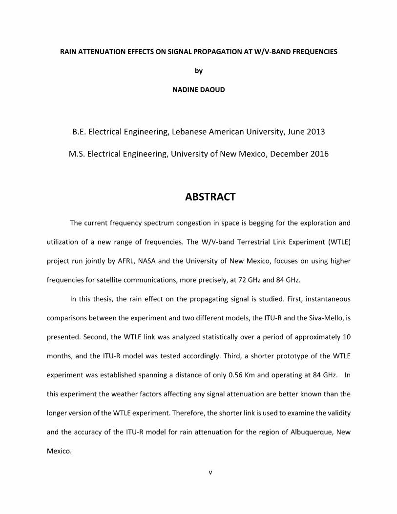
ABSTRACT
The current frequency spectrum congestion in space is begging for the exploration and
utilization of a new range of frequencies. The W/V-‐band Terrestrial Link Experiment (WTLE)
project run jointly by AFRL, NASA and the University of New Mexico, focuses on using higher
frequencies for satellite communications, more precisely, at 72 GHz and 84 GHz.
In this thesis, the rain effect on the propagating signal is studied. First, instantaneous
comparisons between the experiment and two different models, the ITU-‐R and the Siva-‐Mello, is
presented. Second, the WTLE link was analyzed statistically over a period of approximately 10
months, and the ITU-‐R model was tested accordingly. Third, a shorter prototype of the WTLE
experiment was established spanning a distance of only 0.56 Km and operating at 84 GHz. In
this experiment the weather factors affecting any signal attenuation are better known than the
longer version of the WTLE experiment. Therefore, the shorter link is used to examine the validity
and the accuracy of the ITU-‐R model for rain attenuation for the region of Albuquerque, New
Mexico.
vi
Table of Contents List of Figures ...................................................................................................................... ix
List of Tables ....................................................................................................................... xi
Chapter 1 – Introduction ............................................................................................. 1
Chapter 2 -‐ Experiment Setup and Data Manipulation ................................................. 2
Transmitter .......................................................................................................................... 3
Receiver ............................................................................................................................... 5
Disdrometer ......................................................................................................................... 6
Albuquerque’s Weather Characteristics ............................................................................... 7
Chapter 3 – Instantaneous Analysis of the WTLE Link .................................................. 9
Overview ............................................................................................................................. 9
Theoretical Model .............................................................................................................. 10
ITU-‐R Model .......................................................................................................................... 10
Silva-‐Mello Model ................................................................................................................. 11
Comparisons and Results ................................................................................................... 12
Case One ............................................................................................................................... 12
Case Two ............................................................................................................................... 15
Case Three ............................................................................................................................ 17
Case Four .............................................................................................................................. 20
Summary ........................................................................................................................... 22
Chapter 4 – General Analysis of the WTLE Link ........................................................... 23
Overview ........................................................................................................................... 23
Theoretical Model .............................................................................................................. 23
vii
ITU-‐R P.838-‐3 ........................................................................................................................ 24
ITU-‐R P.530 ........................................................................................................................... 24
Experimental Procedure ..................................................................................................... 26
Calculated Attenuation ......................................................................................................... 26
Measured Attenuation ......................................................................................................... 26
Comparisons and Results ................................................................................................... 28
Calculated Attenuation ......................................................................................................... 28
Measured Attenuation ......................................................................................................... 30
Results Analysis .................................................................................................................... 33
72 GHz vs. 84 GHz ................................................................................................................. 34
Summary ........................................................................................................................... 36
Chapter 5 – Short Link Prototype ................................................................................ 37
Overview ........................................................................................................................... 37
Comparisons and Results ................................................................................................... 38
Calculated Attenuation ......................................................................................................... 38
Measured Attenuation ......................................................................................................... 39
Results Analysis .................................................................................................................... 41
Fitting of ITU-‐R Model ........................................................................................................ 42
Chapter 6 – Conclusion ............................................................................................... 45
References ................................................................................................................. 46
Appendix A ................................................................................................................ 48
Matlab Code for the WTLE Link Statistical Analysis ............................................................. 48
Appendix B ................................................................................................................ 54
viii
Matlab Code for the Short Link Statistical Analysis ............................................................. 54
ix
List of Figures
Figure 2.1. WTLE Experiment Path Geometry ................................................................................ 2
Figure 2.2. Transmitter ................................................................................................................... 4
Figure 2.3. Transmitter Site ............................................................................................................ 4
Figure 2.4. Receiver ........................................................................................................................ 5
Figure 2.5. Receiver Site ................................................................................................................. 6
Figure 2.6. Disdrometer ................................................................................................................. 6
Figure 3.1. Region of Interest for the Rain Distribution ............................................................... 10
Figure 3.2. Radar Image on October 10, 2015 at 04:05 GMT. The blue circle corresponds to the
7.438 Km ITU-‐R radius, and the magenta circle corresponds to the 5.509 Km Silva-‐Mello
radius. ................................................................................................................................... 13
Figure 3.3. ITU-‐R and Silva-‐Mello Attenuations at 72 GHz on October 10, 2015 at 04:05 GMT .. 14
Figure 3.4. Radar Image on October 10, 2015 at 01:45 GMT ....................................................... 15
Figure 3.5. ITU-‐R and Silva-‐Mello Attenuations at 72 GHz on October 10, 2015 at 01:45 GMT .. 16
Figure 3.6. ITU-‐R and Silva-‐Mello Attenuations at 84 GHz on October 10, 2015 at 01:45 GMT .. 16
Figure 3.7. Radar Image on November 4, 2015 at 22:30 GMT. The blue circle corresponds to the
10.13 Km ITU-‐R radius, and the magenta circle corresponds to the 7.556 Km Silva-‐Mello
radius. ................................................................................................................................... 18
Figure 3.8. ITU-‐R and Silva-‐Mello Attenuations at 72 GHz on October 4, 2015 at 22:30 GMT .... 19
Figure 3.9. Radar Image on November 17, 2015 at 00:10 GMT ................................................... 20
Figure 3.10. ITU-‐R and Silva-‐Mello Attenuations at 72 GHz on November 17, 2015 at 00:10 GMT
.............................................................................................................................................. 21
x
Figure 3.11. ITU-‐R and Silva-‐Mello Attenuations at 84 GHz on November 17, 2015 at 00:10 GMT
.............................................................................................................................................. 21
Figure 4.1. WTLE Link Rain Rate Cumulative Distribution Function ............................................. 29
Figure 4.2. WTLE Link Total Measured Received Power Cumulative Distribution Function at 72
GHz ....................................................................................................................................... 30
Figure 4.3. WTLE Link Total Measured Received Power Cumulative Distribution Function at 84
GHz ....................................................................................................................................... 32
Figure 5.1. Short Link Experiment Location .................................................................................. 38
Figure 5.2. Short Link Rain Rate Cumulative Distribution Function ............................................. 39
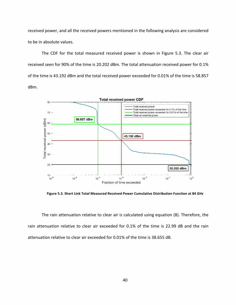
Figure 5.3. Short Link Total Measured Received Power Cumulative Distribution Function at 84
GHz ....................................................................................................................................... 40
Figure 5.4. Rain Attenuation as a Function of Rain Rate .............................................................. 43
xi
List of Tables
Table 2.1. Transmitter Specifications ............................................................................................. 3
Table 2.2. Receiver Specifications .................................................................................................. 5
Table 2.3. Rain Rates Categories .................................................................................................... 7
Table 2.4. Rainfall Distribution According to Months in Albuquerque ........................................... 7
Table 4.1. ITU-‐R P.530 Characteristics .......................................................................................... 25
Table 4.2. WTLE Link Calculated Attenuation Summary .............................................................. 29
Table 4.3. WTLE Link Measured Attenuation at 72 GHz Summary .............................................. 31
Table 4.4. WTLE Link Measured Attenuation at 84 GHz Summary .............................................. 32
Table 4.5. WTLE Link Comparison of ITU-‐R and Experimental Results at 72 GHz ........................ 33
Table 4.6. WTLE Link Comparison of ITU-‐R and Experimental Results at 84 GHz ........................ 34
Table 4.7. WTLE Link Clear Air Attenuation Comparison ............................................................. 35
Table 4.8. WTLE Link Rain Attenuation Relative to Clear Air Comparison ................................... 35
Table 5.1. Short Link Comparison of ITU-‐R and Experimental Results ......................................... 41
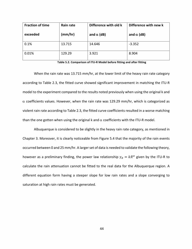
Table 5.2. Comparison of ITU-‐R Model before fitting and after fitting ........................................ 44
1
Chapter 1 – Introduction
The millimeter wave spectrum occupies the 30 GHz to 300 GHz frequency band. When
compared to microwaves, millimeter waves have many advantages some of which are broader
bandwidth, smaller components in the system, reduction in the multipath effects, and selective
atmospheric attenuation. However, the propagation in the millimeter wave band is highly
affected by climate conditions, and rain in particular [1]. Many models have been used to predict
rain attenuation effects on signal propagation for lower frequencies [2]. However, the W/V-‐band
windows have recently emerged as viable communication bands and are currently under
consideration for being used for satellite communication purposes. Thus, existing models [7, 9,
12] have not been tested or proven to work on these frequencies of operation. In order to have
a clear understanding about the climate conditions effects on the communication in the W/V-‐
band, specifically at 72 GHz and 84 GHz, the WTLE (W/V-‐band Terrestrial Link Experiment) was
created. The ultimate goal of this experiment is to determine if existing rain models, would
predict accurately the attenuation based on the rain conditions, or if there is a need to create a
new model designed specifically for this experiment.
Many rain attenuation models have been developed throughout the years, and after
careful consideration, the ITU-‐R model for rain attenuation and the Silva-‐Mello model were
selected for the purpose of comparison with our WTLE experiment.
2
Chapter 2 -‐ Experiment Setup and Data Manipulation
The WTLE experiment was set up and started running on September 3rd, 2015. It
represents a communication link having a transmitter on the Sandia Peak at an altitude of 3.225
km above sea level, and a receiver on the top of the COSMIAC building at the University of New
Mexico at an altitude of 1.619 km above sea level. Both are located in Albuquerque, NM. The
path length between the transmitter and the receiver is 23.5 km, with a resulting slant angle of
4.16o. The overall path geometry is shown in Figure 2.1.
Figure 2.1. WTLE Experiment Path Geometry
The transmitter and the receiver both operate at two different channels to allow the
comparison of the 72 GHz and the 84 GHz bands under the same climate conditions. A weather
station, and a disdrometer were installed at the receiver station as well. A signal is sent from the
3
transmitter station, and the power received is recorded at the receiver station. The availability
of all these different types of data is key for analyzing the experiment and understanding the
climate effects on the propagating signals, as well as checking the validity of the models selected
with regards to predicting attenuation.
Transmitter
The technical specifications of the transmitter located at the top of the Sandia Mountains
are given in Table 2.1 [3].
Parameter V-‐Band W-‐Band
Operating frequency 72 GHz 84 GHz
Antenna Diameter 8.89 cm 8.89 cm
Polarization LHCP LHCP
Antenna Gain 33 dB 34 dB
Antenna Half-‐Power Beamwidth 3.6o (E/H) 3.2o (E) / 3.0o (H)
Effective Isotropic Radiated
Power (with 5 dB Attenuator)
41.1 dBm 40.4 dBm
Table 2.1. Transmitter Specifications
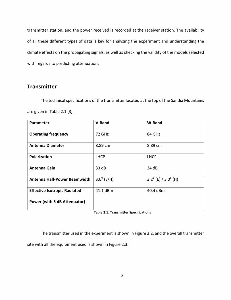
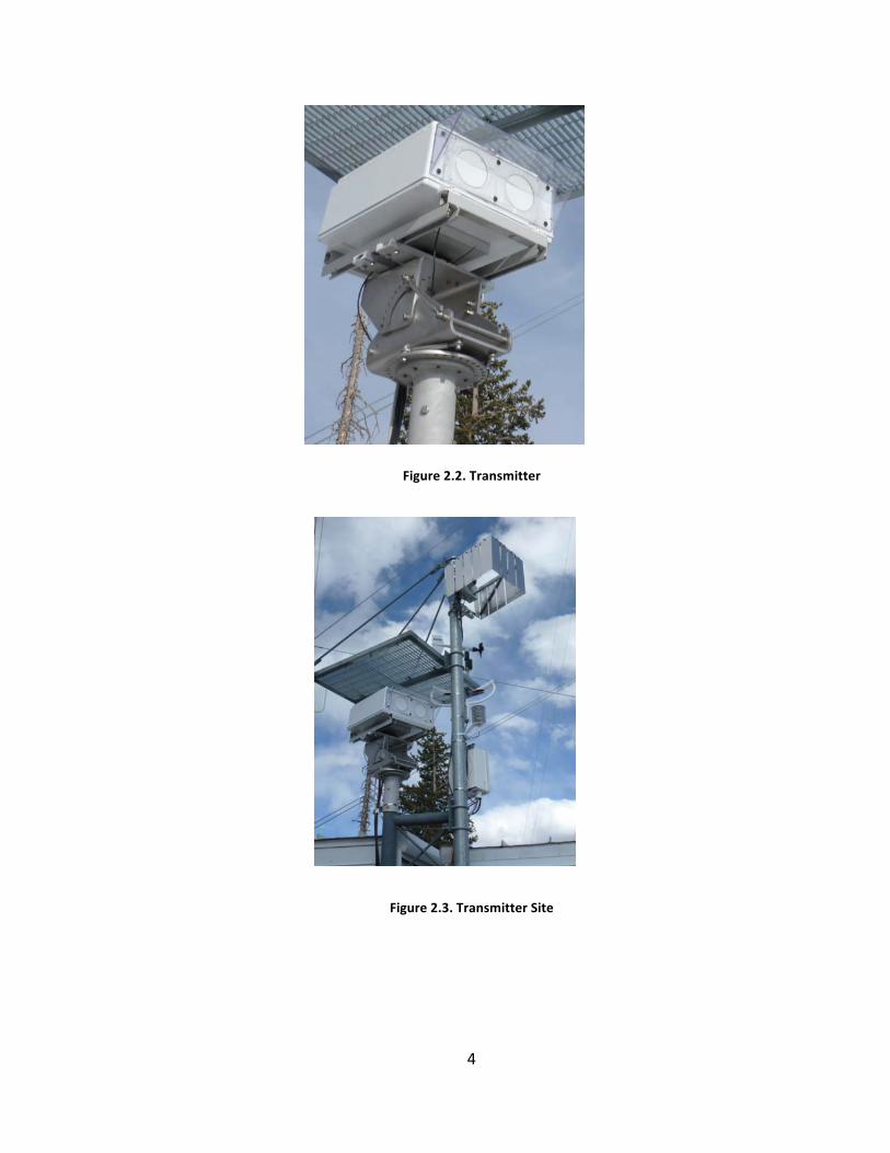
The transmitter used in the experiment is shown in Figure 2.2, and the overall transmitter
site with all the equipment used is shown in Figure 2.3.
4
Figure 2.2. Transmitter
Figure 2.3. Transmitter Site

5
Receiver
The technical specifications of the receiver located at the top of the COSMIAC Building
are given in Table 2.2 [3].
Parameter V-‐Band W-‐Band
Operating Frequency 72 GHz 84 GHz
Antenna Diameter 0.6 m 0.6 m
Polarization LHCP & RHCP LHCP & RHCP
Antenna Gain 50.9 dB 52.2 dB
Antenna Half-‐Power Beamwidth 0.486 0.417
Measurement Rate 10 Hz 10 Hz
Noise Floor -‐75 dBm -‐80 dBm
Table 2.2. Receiver Specifications
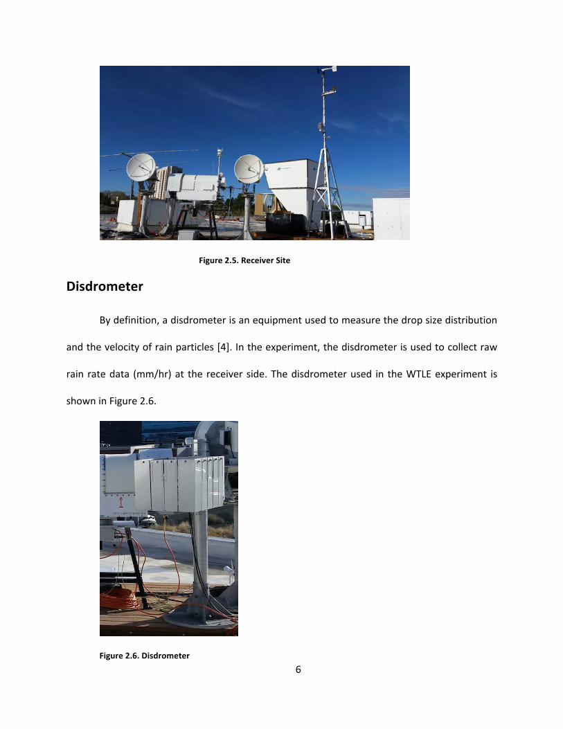
The receivers used in the experiment are shown in Figure 2.4, and the overall receiver site
with all the equipment used is shown in Figure 2.5.
Figure 2.4. Receiver
6
Figure 2.5. Receiver Site
Disdrometer
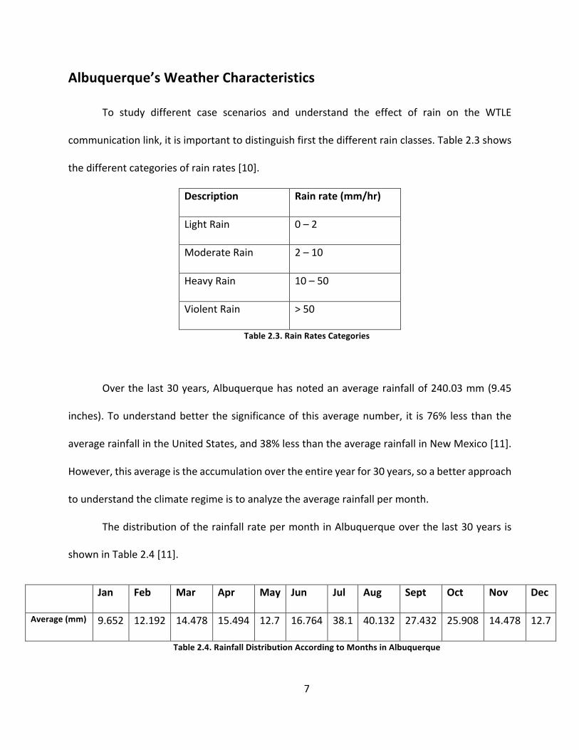
By definition, a disdrometer is an equipment used to measure the drop size distribution
and the velocity of rain particles [4]. In the experiment, the disdrometer is used to collect raw
rain rate data (mm/hr) at the receiver side. The disdrometer used in the WTLE experiment is
shown in Figure 2.6.
Figure 2.6. Disdrometer
7
Albuquerque’s Weather Characteristics
To study different case scenarios and understand the effect of rain on the WTLE
communication link, it is important to distinguish first the different rain classes. Table 2.3 shows
the different categories of rain rates [10].
Description Rain rate (mm/hr)
Light Rain 0 – 2
Moderate Rain 2 – 10
Heavy Rain 10 – 50
Violent Rain > 50
Table 2.3. Rain Rates Categories
Over the last 30 years, Albuquerque has noted an average rainfall of 240.03 mm (9.45
inches). To understand better the significance of this average number, it is 76% less than the
average rainfall in the United States, and 38% less than the average rainfall in New Mexico [11].
However, this average is the accumulation over the entire year for 30 years, so a better approach
to understand the climate regime is to analyze the average rainfall per month.
The distribution of the rainfall rate per month in Albuquerque over the last 30 years is
shown in Table 2.4 [11].
Jan Feb Mar Apr May Jun Jul Aug Sept Oct Nov Dec
Average (mm) 9.652 12.192 14.478 15.494 12.7 16.764 38.1 40.132 27.432 25.908 14.478 12.7
Table 2.4. Rainfall Distribution According to Months in Albuquerque
8
Therefore, Albuquerque is at the lower bound of the heavy rain category, since for most
of the months, the rain average is slightly greater than 10 mm/hr. The rain is mostly intense only
between July and October.
9
Chapter 3 – Instantaneous Analysis of the WTLE Link
Overview
Since the experiment was fairly new, the first approach to analyze its aspects was to study
instantaneous rain event moments, that is, choose specific days, hours, and minutes of the day
where rain was recorded by the disdrometer. However, as mentioned earlier, the disdrometer
gives information for the region around the receiver only, thus the rain conditions along the 23
Km path were unknown except for the receiver area. Therefore, external references such as the
Next Generation Radar (NEXRAD) [5] and the National Oceanic and Atmospheric Administration
(NOAA) weather and climate toolkit [6] were used to check the rain conditions throughout the
path. The challenge was to find specific points in time when it was actually raining only in the
vicinity of the receiver, and not raining anywhere else along the path, to match the rain event
recorded by the disdrometer with the rain conditions along the path, which would allow an
accurate test of the models.
To elaborate more on this matter, one of the major inputs for the ITU-‐R model and the
Silva-‐Mello model is the rain rate, so the rain rate used was the one recorded by the disdrometer.
On the other hand, the attenuation measured at the receiver side was used to test the accuracy
of the attenuation calculated using the models. However, the attenuation measured is affected
by all the rain events throughout the path, not only the ones caught by the disdrometer. So to
make sure that the rain rate recorded by the disdrometer describes accurately the rain rate
affecting the signal, specific points in time where the rain was concentrated around the receiver
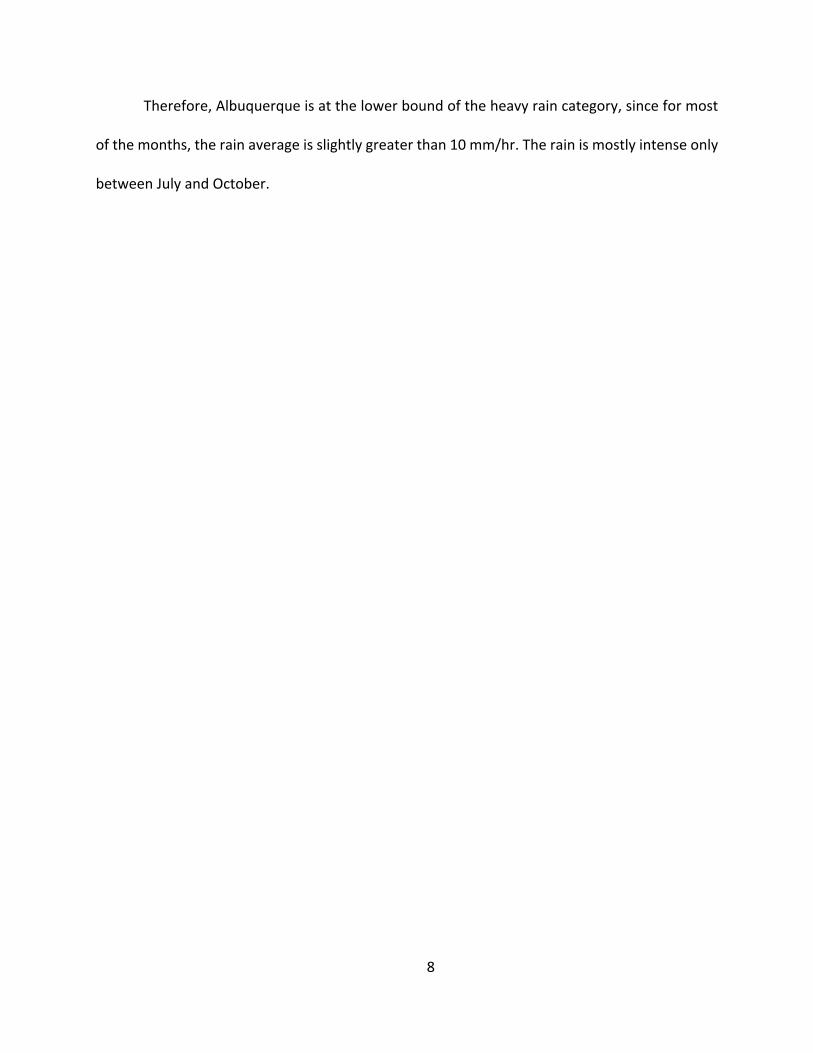
10
only should be used. Figure 3.1 shows a scale to describe the rain distribution of most interest
and most value to the experiment.
Figure 3.1. Region of Interest for the Rain Distribution
Theoretical Model
ITU-‐R Model
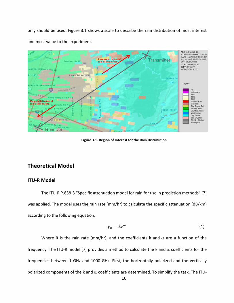
The ITU-‐R P.838-‐3 “Specific attenuation model for rain for use in prediction methods” [7]
was applied. The model uses the rain rate (mm/hr) to calculate the specific attenuation (dB/km)
according to the following equation:
𝛾" = 𝑘𝑅& (1)
Where R is the rain rate (mm/hr), and the coefficients k and a are a function of the
frequency. The ITU-‐R model [7] provides a method to calculate the k and a coefficients for the
frequencies between 1 GHz and 1000 GHz. First, the horizontally polarized and the vertically
polarized components of the k and a coefficients are determined. To simplify the task, The ITU-‐
11
R model gives a table for these values at every frequency. However, these coefficients are proven
to be sufficiently accurate for attenuation prediction for frequencies up to 55 GHz only [8].
Second, these values are used to calculate k and a using the following equations:
𝑘 = 𝑘' + 𝑘) + 𝑘' − 𝑘) 𝑐𝑜𝑠.𝜃 cos 2𝜏 /2 (2)
𝛼 = 𝑘'𝛼' + 𝑘)𝛼) + 𝑘'𝛼' − 𝑘)𝛼) 𝑐𝑜𝑠.𝜃 cos 2𝜏 /2𝑘 (3)
Where q is the path elevation angle and t is the polarization tilt angle relative to the horizontal.
t is equal to 45o for circular polarization.
Silva-‐Mello Model
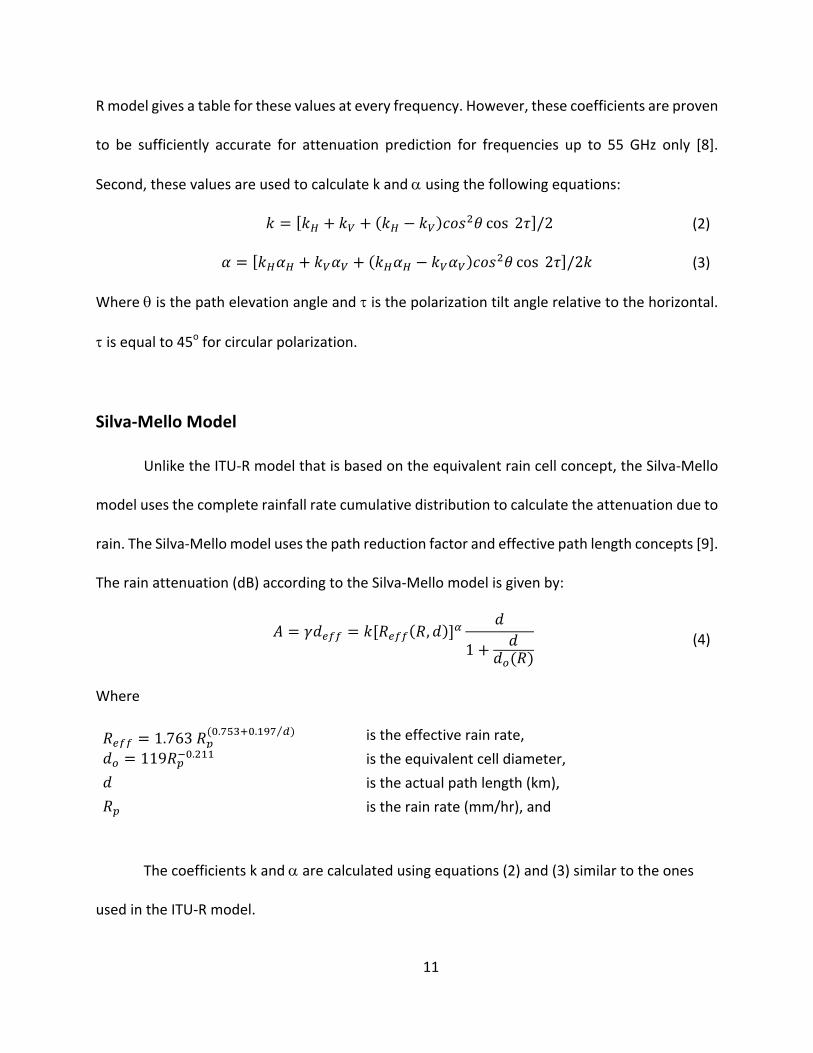
Unlike the ITU-‐R model that is based on the equivalent rain cell concept, the Silva-‐Mello
model uses the complete rainfall rate cumulative distribution to calculate the attenuation due to
rain. The Silva-‐Mello model uses the path reduction factor and effective path length concepts [9].
The rain attenuation (dB) according to the Silva-‐Mello model is given by:
𝐴 = 𝛾𝑑:;; = 𝑘[𝑅:;; 𝑅, 𝑑 ]&𝑑
1 + 𝑑𝑑@(𝑅)
(4)
Where
𝑅:;; = 1.763 𝑅G(H.IJKLH.MNI O) is the effective rain rate,
𝑑@ = 119𝑅GQH..MM is the equivalent cell diameter, 𝑑 is the actual path length (km), 𝑅G is the rain rate (mm/hr), and
The coefficients k and a are calculated using equations (2) and (3) similar to the ones
used in the ITU-‐R model.
12
Comparisons and Results
Different case studies were selected to try to cover as many weather variables as possible,
to understand the effect of each factor on the signal attenuation. At this first stage of the
experiment, and since approximate comparisons were studied, the clear air received power is
assumed to be -‐12 dBm at 72 GHz and -‐16 dBm at 84 GHz. Later in the analysis, accurate
calculations based on a larger range of data set will be shown to determine the clear air
attenuation at 72 GHz and 84 GHz.
Case One
Description
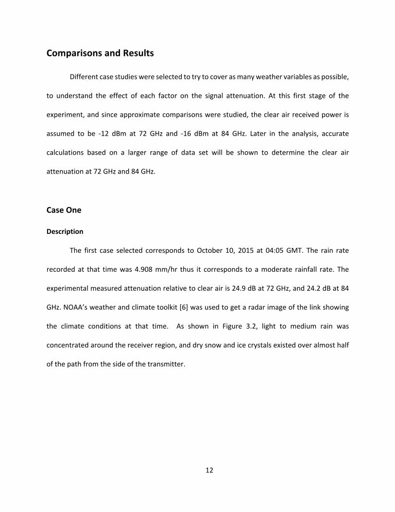
The first case selected corresponds to October 10, 2015 at 04:05 GMT. The rain rate
recorded at that time was 4.908 mm/hr thus it corresponds to a moderate rainfall rate. The
experimental measured attenuation relative to clear air is 24.9 dB at 72 GHz, and 24.2 dB at 84
GHz. NOAA’s weather and climate toolkit [6] was used to get a radar image of the link showing
the climate conditions at that time. As shown in Figure 3.2, light to medium rain was
concentrated around the receiver region, and dry snow and ice crystals existed over almost half
of the path from the side of the transmitter.
13
Figure 3.2. Radar Image on October 10, 2015 at 04:05 GMT. The blue circle corresponds to the 7.438 Km
ITU-‐R radius, and the magenta circle corresponds to the 5.509 Km Silva-‐Mello radius.
The 4.908 mm/hr rainfall rate was used as an input for both the ITU-‐R model and the Silva-‐
Mello model. To consider the worst case scenario, this rainfall rate was assumed to be consistent
all over the path, i.e. that it was raining over the 23 Km path with a rainfall rate of 4.908 mm/hr.
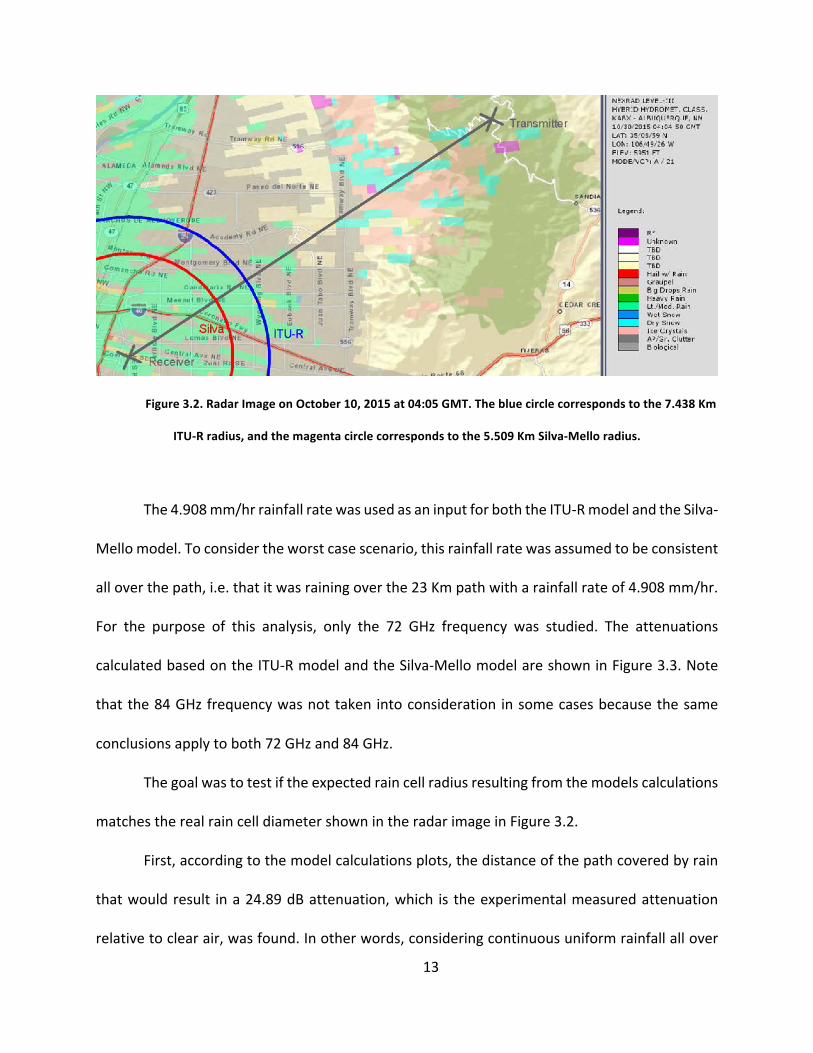
For the purpose of this analysis, only the 72 GHz frequency was studied. The attenuations
calculated based on the ITU-‐R model and the Silva-‐Mello model are shown in Figure 3.3. Note
that the 84 GHz frequency was not taken into consideration in some cases because the same
conclusions apply to both 72 GHz and 84 GHz.
The goal was to test if the expected rain cell radius resulting from the models calculations
matches the real rain cell diameter shown in the radar image in Figure 3.2.
First, according to the model calculations plots, the distance of the path covered by rain
that would result in a 24.89 dB attenuation, which is the experimental measured attenuation
relative to clear air, was found. In other words, considering continuous uniform rainfall all over
14
the path, what is the quantity of rain that would result in a 24.89 dB attenuation relative to clear
air? As shown in Figure 3.3 the rain cell radius according to the ITU-‐R model calculations is 7.438
Km and the rain cell radius according to the Silva-‐Mello model calculations is 5.509 Km.
Second, the two radii are drawn on the radar image as shown in Figure 3.2 to compare
each radius to the actual rain distribution in the area. The blue circle corresponds to the 7.438
Km ITU-‐R radius, and the magenta circle corresponds to the 5.509 Km Silva-‐Mello radius.
Result
According to Figure 3.2, the analysis based on the ITU-‐R model seems to match the
experimental results more than the Silva-‐Mello model since the rain coverage area matches the
light/medium rain area showed by the radar more than the Silva-‐Mello case. However, the dry
snow and ice crystals mentioned earlier were not taken into account in the calculations, and at
that point it was unknown if these factors had any effects on the attenuation or not.
Figure 3.3. ITU-‐R and Silva-‐Mello Attenuations at 72 GHz on October 10, 2015 at 04:05 GMT
15
Case Two
Description
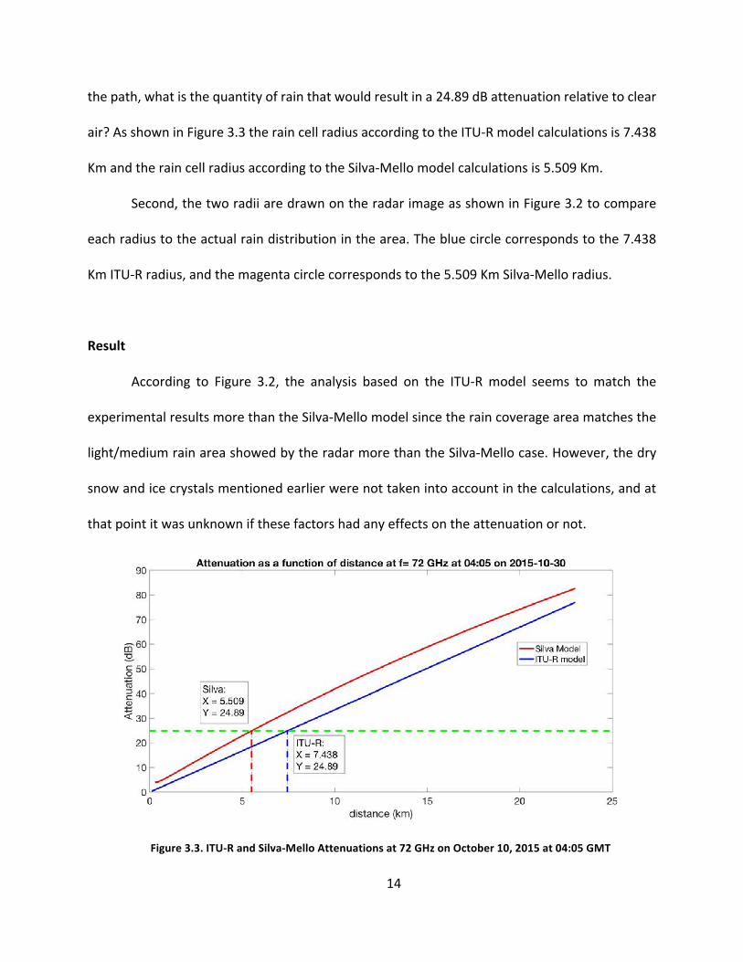
The second case considered corresponds to October 10, 2015 at 01:45 GMT. The rain rate
recorded at that time was 0.064 mm/hr thus it corresponds to a light rainfall rate. The
experimental measured attenuation relative to clear air is 7.40 dB at 72 GHz, and 6.49 dB at 84
GHz. The same procedure as the one described in case 1 was followed. NOAA’s weather and
climate toolkit [6] was used to get a radar image of the link showing the climate conditions at
that time. The radar image in Figure 3.4, shows that light to medium rain was concentrated
around the receiver region, and no other weather factors exist along the path from the
transmitter to the receiver.
Figure 3.4. Radar Image on October 10, 2015 at 01:45 GMT
Just like in case 1, the 0.064 mm/hr rainfall rate was used as an input for both ITU-‐R model
and Silva-‐Mello model. Considering continuous and uniform rainfall along the 23 Km path, the
attenuations calculated based on the ITU-‐R model and the Silva-‐Mello model are shown in Figure
16
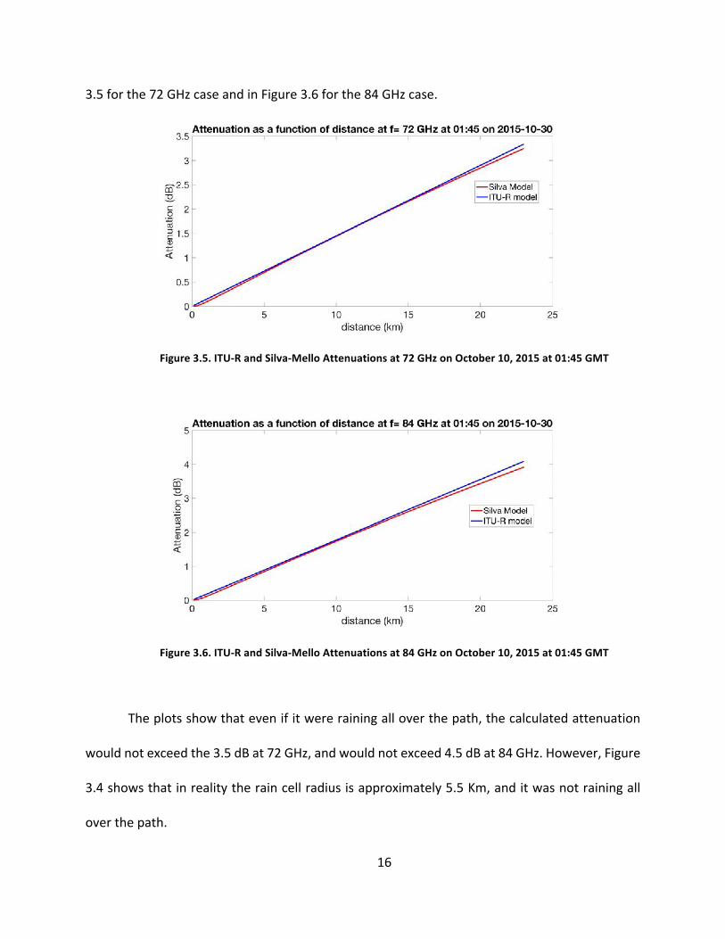
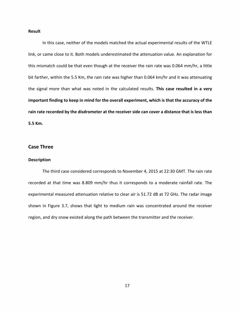
3.5 for the 72 GHz case and in Figure 3.6 for the 84 GHz case.
Figure 3.5. ITU-‐R and Silva-‐Mello Attenuations at 72 GHz on October 10, 2015 at 01:45 GMT
Figure 3.6. ITU-‐R and Silva-‐Mello Attenuations at 84 GHz on October 10, 2015 at 01:45 GMT
The plots show that even if it were raining all over the path, the calculated attenuation
would not exceed the 3.5 dB at 72 GHz, and would not exceed 4.5 dB at 84 GHz. However, Figure
3.4 shows that in reality the rain cell radius is approximately 5.5 Km, and it was not raining all
over the path.
17
Result
In this case, neither of the models matched the actual experimental results of the WTLE
link, or came close to it. Both models underestimated the attenuation value. An explanation for
this mismatch could be that even though at the receiver the rain rate was 0.064 mm/hr, a little
bit farther, within the 5.5 Km, the rain rate was higher than 0.064 km/hr and it was attenuating
the signal more than what was noted in the calculated results. This case resulted in a very
important finding to keep in mind for the overall experiment, which is that the accuracy of the
rain rate recorded by the disdrometer at the receiver side can cover a distance that is less than
5.5 Km.
Case Three
Description
The third case considered corresponds to November 4, 2015 at 22:30 GMT. The rain rate
recorded at that time was 8.809 mm/hr thus it corresponds to a moderate rainfall rate. The
experimental measured attenuation relative to clear air is 51.72 dB at 72 GHz. The radar image
shown in Figure 3.7, shows that light to medium rain was concentrated around the receiver
region, and dry snow existed along the path between the transmitter and the receiver.
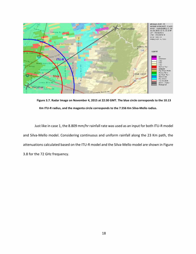
18
Figure 3.7. Radar Image on November 4, 2015 at 22:30 GMT. The blue circle corresponds to the 10.13
Km ITU-‐R radius, and the magenta circle corresponds to the 7.556 Km Silva-‐Mello radius.
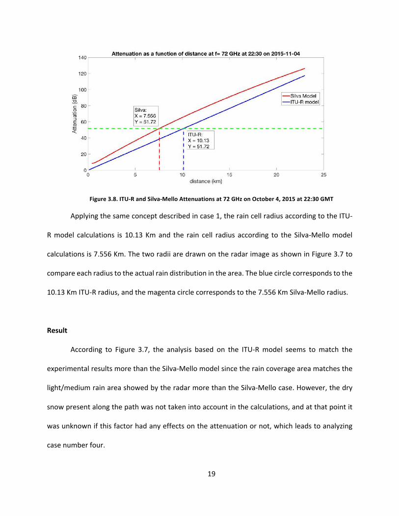
Just like in case 1, the 8.809 mm/hr rainfall rate was used as an input for both ITU-‐R model
and Silva-‐Mello model. Considering continuous and uniform rainfall along the 23 Km path, the
attenuations calculated based on the ITU-‐R model and the Silva-‐Mello model are shown in Figure
3.8 for the 72 GHz frequency.
19
Figure 3.8. ITU-‐R and Silva-‐Mello Attenuations at 72 GHz on October 4, 2015 at 22:30 GMT
Applying the same concept described in case 1, the rain cell radius according to the ITU-‐
R model calculations is 10.13 Km and the rain cell radius according to the Silva-‐Mello model
calculations is 7.556 Km. The two radii are drawn on the radar image as shown in Figure 3.7 to
compare each radius to the actual rain distribution in the area. The blue circle corresponds to the
10.13 Km ITU-‐R radius, and the magenta circle corresponds to the 7.556 Km Silva-‐Mello radius.
Result
According to Figure 3.7, the analysis based on the ITU-‐R model seems to match the
experimental results more than the Silva-‐Mello model since the rain coverage area matches the
light/medium rain area showed by the radar more than the Silva-‐Mello case. However, the dry
snow present along the path was not taken into account in the calculations, and at that point it
was unknown if this factor had any effects on the attenuation or not, which leads to analyzing
case number four.
20
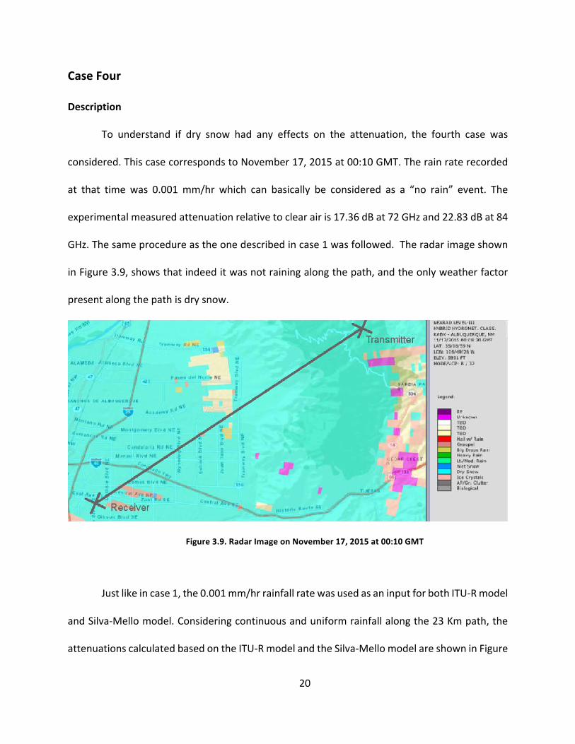
Case Four
Description
To understand if dry snow had any effects on the attenuation, the fourth case was
considered. This case corresponds to November 17, 2015 at 00:10 GMT. The rain rate recorded
at that time was 0.001 mm/hr which can basically be considered as a “no rain” event. The
experimental measured attenuation relative to clear air is 17.36 dB at 72 GHz and 22.83 dB at 84
GHz. The same procedure as the one described in case 1 was followed. The radar image shown
in Figure 3.9, shows that indeed it was not raining along the path, and the only weather factor
present along the path is dry snow.
Figure 3.9. Radar Image on November 17, 2015 at 00:10 GMT
Just like in case 1, the 0.001 mm/hr rainfall rate was used as an input for both ITU-‐R model
and Silva-‐Mello model. Considering continuous and uniform rainfall along the 23 Km path, the
attenuations calculated based on the ITU-‐R model and the Silva-‐Mello model are shown in Figure
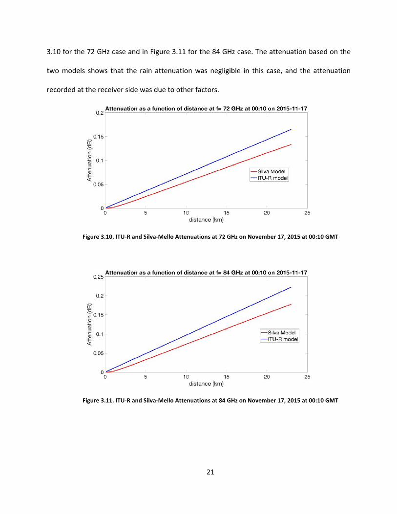
21
3.10 for the 72 GHz case and in Figure 3.11 for the 84 GHz case. The attenuation based on the
two models shows that the rain attenuation was negligible in this case, and the attenuation
recorded at the receiver side was due to other factors.
Figure 3.10. ITU-‐R and Silva-‐Mello Attenuations at 72 GHz on November 17, 2015 at 00:10 GMT
Figure 3.11. ITU-‐R and Silva-‐Mello Attenuations at 84 GHz on November 17, 2015 at 00:10 GMT
22
Result
Since there was no rain, and thus no rain attenuation, and since the only weather factor
that existed along the communication link was the dry snow, it can be established that the
attenuation relative to clear air was due to the dry snow effects in this case. Therefore, if dry
snow exists along the path (in this case and in the previous cases), it cannot be neglected
because it is attenuating the signal.
Summary
Using the instantaneous analysis, none of the two models showed consistent results for
the case studied. Moreover, due to the lack of data availability throughout the link, the data
recorded at the receiver was assumed to be consistent all over the path, which was not accurate
when compared to the actual climate condition.
A conclusion cannot be drawn based on instantaneous specific cases; thus a better
approach would be to analyze the link’s behavior over a long period of time and to examine
statistical results.
23
Chapter 4 – General Analysis of the WTLE Link
Overview
After using the instantaneous analysis to understand the different weather factors that
might affect the signal, a more general analysis was considered to understand the overall
behavior of the link over a certain period of time. The timespan of the following study goes
roughly from October 1st, 2015 to July 15th, 2016. The model under consideration was the ITU-‐R
model for rain attenuation [7, 12]. The rain rate (mm/hr) recorded by the disdrometer, and the
received power were used to compare experimental and theoretical results.
Several analyses were considered:
1) A Comparison of the measured rain attenuation relative to clear air and the calculated
rain attenuation based on the ITU-‐R model [7, 12] exceeded for 0.01% of the time and
0.1% of the time at 72 GHz.
2) A Comparison of the measured rain attenuation relative to clear air and the calculated
rain attenuation based on the ITU-‐R model [7, 12] exceeded for 0.01% of the time and
0.1% of the time at 84 GHz.
3) A Comparison of the experimental results at 72 GHz and 84 GHz.
Theoretical Model
The ITU-‐R procedure used for the following part is a combination of two ITU-‐R models.
The first model [7] calculates the attenuation as a function of distance, and the second model
[12] computes an effective path length to calculate the total attenuation over the region of
24
interest.
ITU-‐R P.838-‐3
The ITU-‐R P.838-‐3 model [7] is the same model used in Chapter 3 for the instantaneous
comparison. The attenuation (dB/Km) is given by the following equation:
𝛾" = 𝑘𝑅& (5)
Where R is the rain rate (mm/hr) exceeded for p% of the time,
k and a are coefficients function of the frequency and they are calculated as described
previously in Chapter 3.
ITU-‐R P.530
The ITU-‐R P.530 model [12] calculates the total attenuation (dB) exceeded for a p% of
time by multiplying the attenuation resulting from the ITU-‐R P.838-‐3 model [7] by an effective
path length as follows:
𝐴G = 𝛾"𝑑:;; (6)
Where 𝛾" is the specific attenuation (dB/Km),
𝑑:;; = 𝑑 × 𝑟 is the effective path length where d (Km) is the actual path length, and r is
a distance factor calculated as shown in equation (7).
25
𝑟 = 1
0.477 𝑑H.VKK𝑅GH.HIK &𝑓H.M.K − 10.579 (1 − exp −0.024𝑑 ) (7)
Where Rp is the rain rate (mm/hr) exceeded for p% of the time,
d is the actual path length (Km),
f is the frequency of operation (GHz)
a is the frequency dependent coefficient.
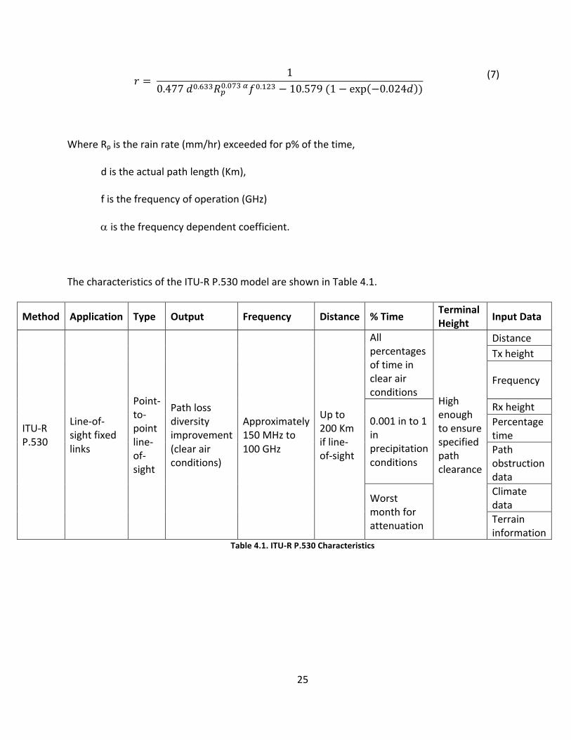
The characteristics of the ITU-‐R P.530 model are shown in Table 4.1.
Method Application Type Output Frequency Distance % Time Terminal Height Input Data
ITU-‐R P.530
Line-‐of-‐sight fixed links
Point-‐to-‐point line-‐of-‐sight
Path loss diversity improvement (clear air conditions)
Approximately 150 MHz to 100 GHz
Up to 200 Km if line-‐of-‐sight
All percentages of time in clear air conditions
High enough to ensure specified path clearance
Distance Tx height
Frequency
0.001 in to 1 in precipitation conditions
Rx height Percentage time Path obstruction data
Worst month for attenuation
Climate data Terrain information
Table 4.1. ITU-‐R P.530 Characteristics
26
Experimental Procedure
Calculated Attenuation
The first part of the experiment was to calculate the total rain attenuation for the WTLE
link using the rain rate and the ITU-‐R model. The calculation was performed according to the
following steps:
1) A cumulative distribution function (CDF) of the rain rate was plotted to show the rain
distribution at the receiver site from October 1st, 2015 till July 15th, 2016.
2) Using the rain rate CDF, the rain rate exceeded for 0.1% of the time and the rain rate
exceeded for 0.01% of the time were found.
3) These rain rate were then inputted simultaneously in equation (3) to calculate the
corresponding attenuation in dB/Km.
4) The total rain attenuation exceeded for 0.1% of the time and the total rain attenuation
exceeded for 0.01% of the time were calculated according to the ITU-‐R model [7, 12] by
multiplying the attenuation in dB/Km by the effective path length as shown in equations
(6) and (7).
Measured Attenuation
The second part of the experiment was to calculate the total rain attenuation for the
WTLE link using the recorded received power at the receiver. Since the rain attenuation was
calculated relative to the clear air attenuation basis, the power of the transmitted signal does not
27
affect the results and is not a point of interest. The calculation was performed according to the
following steps:
1) A cumulative distribution function for the total experimental received power was plotted
for the time period of interest. This CDF is plotted using the absolute values of the
received power, and all the received powers mentioned in the following analysis are
considered to be in absolute values.
2) Using the total received power CDF, the total received power recorded for 90% of the
time was found; this received power corresponds to the clear air received power since it
can be assumed that for more than 90% of the time no rain events are noted on the WTLE
link.
3) Using the total received power CDF, the total received power exceeded for 0.1% of the
time and the total received power exceeded for 0.01% of the time were found.
4) The rain attenuation relative to clear air exceeded for 0.1% and 0.01% of the time were
calculated by subtracting the clear air received power from the total received powers
exceeded for 0.1% and 0.01% of the time correspondingly.
5) The noise floor level is a very important factor to be taken into consideration to make sure
that the data used in the experiment are valid. At 72 GHz the noise floor level is -‐75 dBm
and at 84 GHz the noise floor level is -‐80 dBm. For the purpose of the comparison with the
CDF plot, the noise floors are also used in absolute values. Therefore, any recorded value
below these two thresholds must be evaluated and must fall into one of the two following
categories:
28
Ø The value larger than the threshold (in absolute value) was reached during a rain event,
thus it must be taken into consideration for the statistical analysis of the experiment
as a rain event, however its value was not accurate. In other words, this value was kept
in the statistical analysis and was considered as a flat 75 dBm or 80 dBm received
power depending on the frequency of operation.
Ø The value larger than the threshold (in absolute value) was reached suddenly and for
a relatively short period of time during a clear day event, which means that it was the
result of a failure in the experiment or in the equipment, and thus should be totally
neglected and removed from the analysis.
6) Finally, the dynamic range for the rain event at each frequency was calculated by
subtracting the noise floor level from the clear air received power. Note that any rain
attenuation relative to clear air that exceeded the dynamic range was not a valid value and
was not considered in the analysis.
Comparisons and Results
Calculated Attenuation
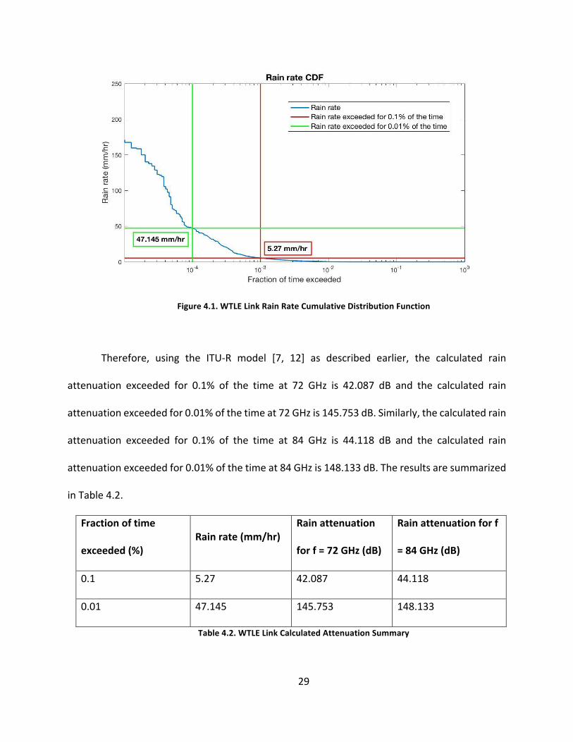
First, the rain attenuation according to the ITU-‐R model was calculated.
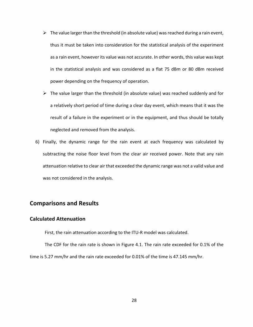
The CDF for the rain rate is shown in Figure 4.1. The rain rate exceeded for 0.1% of the
time is 5.27 mm/hr and the rain rate exceeded for 0.01% of the time is 47.145 mm/hr.
29
Figure 4.1. WTLE Link Rain Rate Cumulative Distribution Function
Therefore, using the ITU-‐R model [7, 12] as described earlier, the calculated rain
attenuation exceeded for 0.1% of the time at 72 GHz is 42.087 dB and the calculated rain
attenuation exceeded for 0.01% of the time at 72 GHz is 145.753 dB. Similarly, the calculated rain
attenuation exceeded for 0.1% of the time at 84 GHz is 44.118 dB and the calculated rain
attenuation exceeded for 0.01% of the time at 84 GHz is 148.133 dB. The results are summarized
in Table 4.2.
Fraction of time
exceeded (%) Rain rate (mm/hr)
Rain attenuation
for f = 72 GHz (dB)
Rain attenuation for f
= 84 GHz (dB)
0.1 5.27 42.087 44.118
0.01 47.145 145.753 148.133
Table 4.2. WTLE Link Calculated Attenuation Summary
30
Measured Attenuation
72 GHz Frequency
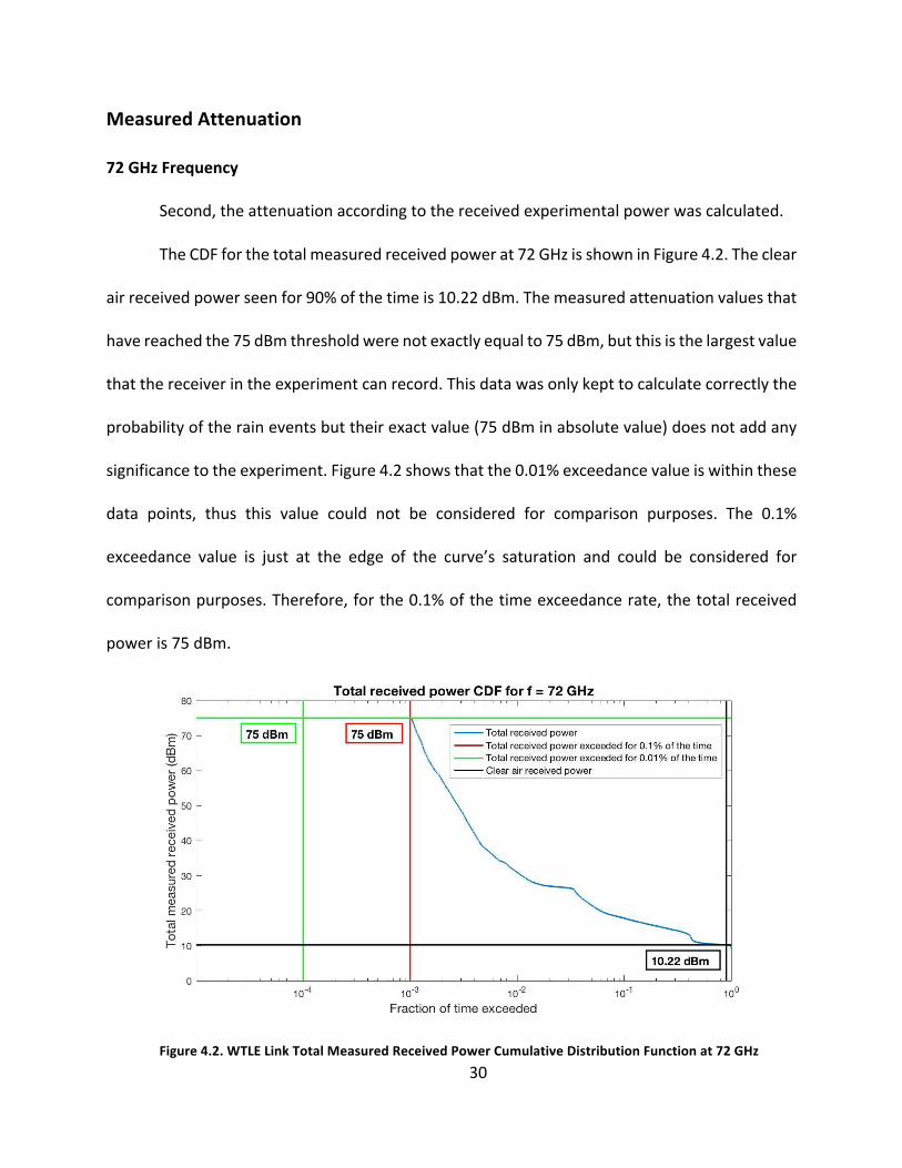
Second, the attenuation according to the received experimental power was calculated.
The CDF for the total measured received power at 72 GHz is shown in Figure 4.2. The clear
air received power seen for 90% of the time is 10.22 dBm. The measured attenuation values that
have reached the 75 dBm threshold were not exactly equal to 75 dBm, but this is the largest value
that the receiver in the experiment can record. This data was only kept to calculate correctly the
probability of the rain events but their exact value (75 dBm in absolute value) does not add any
significance to the experiment. Figure 4.2 shows that the 0.01% exceedance value is within these
data points, thus this value could not be considered for comparison purposes. The 0.1%
exceedance value is just at the edge of the curve’s saturation and could be considered for
comparison purposes. Therefore, for the 0.1% of the time exceedance rate, the total received
power is 75 dBm.
Figure 4.2. WTLE Link Total Measured Received Power Cumulative Distribution Function at 72 GHz
31
The rain attenuation relative to clear air is calculated as follows:
𝑟𝑎𝑖𝑛 𝑎𝑡𝑡𝑒𝑛𝑢𝑎𝑡𝑖𝑜𝑛 𝑟𝑒𝑙𝑎𝑡𝑖𝑣𝑒 𝑡𝑜 𝑐𝑙𝑒𝑎𝑟 𝑎𝑖𝑟 = 𝑡𝑜𝑡𝑎𝑙 𝑟𝑒𝑐𝑒𝑖𝑣𝑒𝑑 𝑝𝑜𝑤𝑒𝑟 − 𝑐𝑙𝑒𝑎𝑟 𝑎𝑖𝑟 𝑟𝑒𝑐𝑒𝑖𝑣𝑒𝑑 𝑝𝑜𝑤𝑒𝑟 (8)
Therefore, the rain attenuation relative to clear air exceeded for 0.1% of the time is 64.78
dB. The results are summarized in Table 4.3.
Fraction of time exceeded Total received power
for f = 72 GHz (dBm)
Rain attenuation relative to
clear air for f = 72 GHz (dB)
0.1 75 64.78
Table 4.3. WTLE Link Measured Attenuation at 72 GHz Summary
Finally, the dynamic range of the rain event under consideration is calculated as follows:
𝑑𝑦𝑛𝑎𝑚𝑖𝑐 𝑟𝑎𝑛𝑔𝑒 = 𝑐𝑙𝑒𝑎𝑟 𝑎𝑖𝑟 𝑟𝑒𝑐𝑒𝑖𝑣𝑒𝑑 𝑝𝑜𝑤𝑒𝑟 − 𝑛𝑜𝑖𝑠𝑒 𝑓𝑙𝑜𝑜𝑟 (9)
𝑑𝑦𝑛𝑎𝑚𝑖𝑐 𝑟𝑎𝑛𝑔𝑒 = 10.22 − (−75)
𝑑𝑦𝑛𝑎𝑚𝑖𝑐 𝑟𝑎𝑛𝑔𝑒 = 85.22 𝑑𝐵
84 GHz Frequency
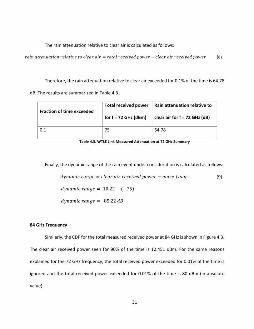
Similarly, the CDF for the total measured received power at 84 GHz is shown in Figure 4.3.
The clear air received power seen for 90% of the time is 12.451 dBm. For the same reasons
explained for the 72 GHz frequency, the total received power exceeded for 0.01% of the time is
ignored and the total received power exceeded for 0.01% of the time is 80 dBm (in absolute
value).
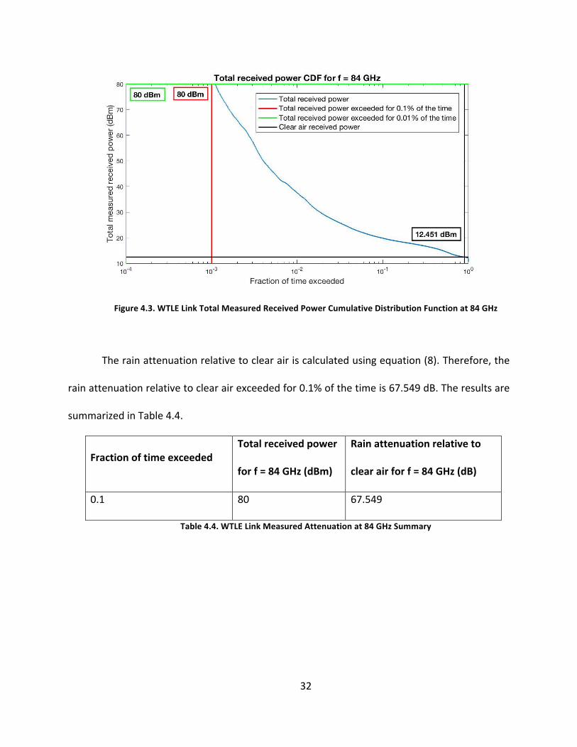
32
Figure 4.3. WTLE Link Total Measured Received Power Cumulative Distribution Function at 84 GHz
The rain attenuation relative to clear air is calculated using equation (8). Therefore, the
rain attenuation relative to clear air exceeded for 0.1% of the time is 67.549 dB. The results are
summarized in Table 4.4.
Fraction of time exceeded Total received power
for f = 84 GHz (dBm)
Rain attenuation relative to
clear air for f = 84 GHz (dB)
0.1 80 67.549
Table 4.4. WTLE Link Measured Attenuation at 84 GHz Summary
33
Next, the dynamic range is calculated using equation (9).
𝑑𝑦𝑛𝑎𝑚𝑖𝑐 𝑟𝑎𝑛𝑔𝑒 = 𝑐𝑙𝑒𝑎𝑟 𝑎𝑖𝑟 𝑟𝑒𝑐𝑒𝑖𝑣𝑒𝑑 𝑝𝑜𝑤𝑒𝑟 − 𝑛𝑜𝑖𝑠𝑒 𝑓𝑙𝑜𝑜𝑟 (9)
𝑑𝑦𝑛𝑎𝑚𝑖𝑐 𝑟𝑎𝑛𝑔𝑒 = 12.451 − (−80)
𝑑𝑦𝑛𝑎𝑚𝑖𝑐 𝑟𝑎𝑛𝑔𝑒 = 90.451 𝑑𝐵
Results Analysis
The computed rain attenuation using the ITU-‐R model and the measured attenuation
calculated using experimental data were compared to check the validity of the ITU-‐R model for
the WTLE link. The results corresponding to the 0.1% of the time exceedance rate were compared
only, because the ones corresponding to the 0.01% of the time exceedance rate showed to be
out of bound. The difference is calculated according to equation (10). The results are summarized
in Table 4.5 for the 72 GHz values and Table 4.6 for the 84 GHz values.
𝐷𝑖𝑓𝑓𝑒𝑟𝑒𝑛𝑐𝑒 = 𝐸𝑥𝑝𝑒𝑟𝑖𝑚𝑒𝑛𝑡𝑎𝑙 𝑟𝑎𝑖𝑛 𝑎𝑡𝑡𝑒𝑛𝑢𝑎𝑡𝑖𝑜𝑛 − 𝐼𝑇𝑈𝑅 𝑟𝑎𝑖𝑛 𝑎𝑡𝑡𝑒𝑛𝑢𝑎𝑡𝑖𝑜𝑛 (10)
Rain rate
(mm/hr)
ITU-‐R rain
attenuation (dB)
Experimental rain
attenuation (dB)
Attenuation
difference (dB)
5.27 42.087 64.78 22.693
Table 4.5. WTLE Link Comparison of ITU-‐R and Experimental Results at 72 GHz
34
Rain rate
(mm/hr)
ITU-‐R rain
attenuation (dB)
Experimental rain
attenuation (dB)
Attenuation
difference (dB)
5.27 44.118 67.549 23.431
Table 4.6. WTLE Link Comparison of ITU-‐R and Experimental Results at 84 GHz
For both frequencies of operation, the ITU-‐R showed optimistic results when compared
to the experiment. However, the interesting finding is that, for the same rain rate, the
inconsistency of the ITU-‐R model compared to the experimental results was consistent between
the two frequencies of operation. Though, as noted in Chapter 3, the disdrometer is giving
information about the rain rate only at the receiver site, and the validity of this data covers much
less than 5.5Km of the 23 Km link. This means that the high attenuation recorded by the
experiment could be due to more severe rain events that were not caught by the disdrometer,
whereas the rain attenuation calculated using the ITU-‐R model resulted from using the low rain
rate noted by the disdrometer. Therefore, this could have caused having the optimistic ITU-‐R
results compared to the experimental ones. More analysis is performed in Chapter 5, to examine
the accuracy of the ITU-‐R model for the WTLE experiment.
72 GHz vs. 84 GHz
The experiment analysis was done for the 72 GHz and 84 GHz frequencies simultaneously.
However, if a relation for the signal behavior between these two frequencies is found, the
experiment can be done for just one of the frequencies, and the result can be extrapolated for
the second frequency, which would consequently save time and resources.
35
For the purpose of this analysis, only the experimental results were used. In addition, only
the results corresponding to the 0.1% of the time exceedance rate were compared because they
were the only ones proven to be valid and within the dynamic range of the experiment.
Therefore, two factors were compared for the two frequencies: the clear air received
power (Table 4.7) according to equation (11) , and the rain attenuation relative to clear air (Table
4.8). The difference is calculated according to equation (12).
𝐷𝑖𝑓𝑓𝑒𝑟𝑒𝑛𝑐𝑒 = 𝑅𝑒𝑐𝑒𝑖𝑣𝑒𝑑 𝑝𝑜𝑤𝑒𝑟 𝑎𝑡 84 𝐺𝐻𝑧 − 𝑅𝑒𝑐𝑒𝑖𝑣𝑒𝑑 𝑝𝑜𝑤𝑒𝑟 𝑎𝑡 72 𝐺𝐻𝑧 (11)
𝐷𝑖𝑓𝑓𝑒𝑟𝑒𝑛𝑐𝑒 = 𝐴𝑡𝑡𝑒𝑛𝑢𝑎𝑡𝑖𝑜𝑛 𝑎𝑡 84 𝐺𝐻𝑧 − 𝐴𝑡𝑡𝑒𝑛𝑢𝑎𝑡𝑖𝑜𝑛 𝑎𝑡 72 𝐺𝐻𝑧 (12)
Received power at
f = 72 GHz (dBm)
Received power at
f = 84 GHz (dBm)
Received power
difference (dBm)
10.22 12.451 2.231
Table 4.7. WTLE Link Clear Air Attenuation Comparison
Attenuation at f =
72 GHz (dB)
Attenuation at f
= 84 GHz (dB)
Attenuation
difference (dB)
64.78 67.549 2.769
Table 4.8. WTLE Link Rain Attenuation Relative to Clear Air Comparison
36
Table 4.7 and Table 4.8 show that the clear air received power at 84 GHz was larger than
the one at 72 GHz by 2.231 dBm, and the rain attenuation relative to clear air at 84 GHz was
larger than the one at 72 GHz by 2.769 dB.
Consequently, if the 84 GHz frequency is chosen to perform the experiment, one would
confidently say that this would cover the worst case scenario. The rain attenuation value relative
to clear air recorded for the 84 GHz link, will be always greater than the one at 72 GHz by about
2.769 dB under the same experimental conditions.
Summary
Using the statistical approach for the WTLE link showed that the ITU-‐R model does not
match with the experiment conducted in Albuquerque, New Mexico. Nevertheless, this
conclusion could not be validated due to the lack of data along the communication path.
Consequently, further analysis needs to be performed.
Note: Recently, it has been noted that some inconsistencies in the experiment are not
permitting a correct estimation for the clear air received power value. However, it is known
that once corrections are made, and exact clear air received power value can be calculated, the
gap between the theoretical and experimental results will increase. Therefore, since the model
does not match with the experiment now, it will absolutely not match with the experiment
after the corrections are made. Moreover, the method presented can be applied to any future
data collected, so the theory and the procedure would be the same for any data set.
37
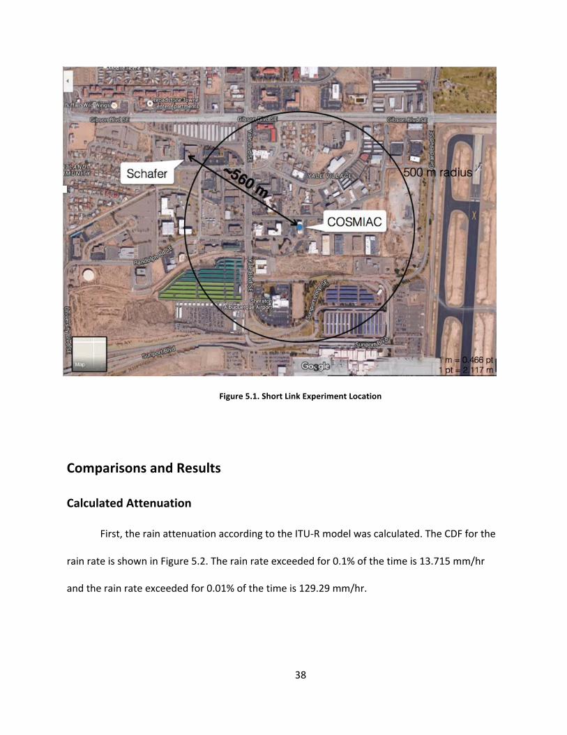
Chapter 5 – Short Link Prototype
Overview
To overcome the ambiguity caused by the missing data over the 23 Km link, and to have
better control over the experiment, a short link of 0.56 Km operating at 84 GHz was built. The 84
GHz receiver located at the top of the COSMIAC building that was used for the WTLE experiment
was redirected to serve as the receiver for the short link experiment. An 84 GHz transmitter was
placed on the top of the Schafer Corporation building. The equipment locations are shown in
Figure 5.1. Rain rate and received power are still recorded at the receiver site. In this case, the
rain rate seen at the receiver can be assumed to be consistent for the overall link because the
communication path is short, and statistical study is under consideration. The data used for the
short link analysis spans roughly from August 3, 2016 till September 30, 2016. The same ITU-‐R
model [7, 12] used in the Long link analysis was tested in this short link experiment. Even though
the sample size is small, it is sufficient in order to perform a preliminary test to check whether
the ITU-‐R model is accurate for the region of Albuquerque or not.
In this chapter, two analyses were performed:
1) A Comparison of the measured rain attenuation relative to clear air and the calculated
rain attenuation based on the ITU-‐R model [7, 12] exceeded for 0.01% of the time and
0.1% of the time at 84 GHz.
2) A Comparison of the measured rain attenuation relative to clear air and the calculated
rain attenuation based on the ITU-‐R model as a function of the rain rate, and finding new
k and a coefficients for the ITU-‐R model to fit it to the experimental results.
38
Figure 5.1. Short Link Experiment Location
Comparisons and Results
Calculated Attenuation
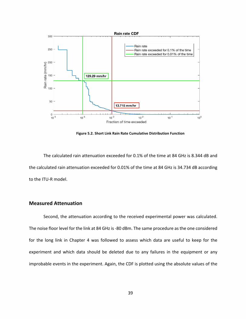
First, the rain attenuation according to the ITU-‐R model was calculated. The CDF for the
rain rate is shown in Figure 5.2. The rain rate exceeded for 0.1% of the time is 13.715 mm/hr
and the rain rate exceeded for 0.01% of the time is 129.29 mm/hr.
39
Figure 5.2. Short Link Rain Rate Cumulative Distribution Function
The calculated rain attenuation exceeded for 0.1% of the time at 84 GHz is 8.344 dB and
the calculated rain attenuation exceeded for 0.01% of the time at 84 GHz is 34.734 dB according
to the ITU-‐R model.
Measured Attenuation
Second, the attenuation according to the received experimental power was calculated.
The noise floor level for the link at 84 GHz is -‐80 dBm. The same procedure as the one considered
for the long link in Chapter 4 was followed to assess which data are useful to keep for the
experiment and which data should be deleted due to any failures in the equipment or any
improbable events in the experiment. Again, the CDF is plotted using the absolute values of the
40
received power, and all the received powers mentioned in the following analysis are considered
to be in absolute values.
The CDF for the total measured received power is shown in Figure 5.3. The clear air
received seen for 90% of the time is 20.202 dBm. The total attenuation received power for 0.1%
of the time is 43.192 dBm and the total received power exceeded for 0.01% of the time is 58.857
dBm.
Figure 5.3. Short Link Total Measured Received Power Cumulative Distribution Function at 84 GHz
The rain attenuation relative to clear air is calculated using equation (8). Therefore, the
rain attenuation relative to clear air exceeded for 0.1% of the time is 22.99 dB and the rain
attenuation relative to clear air exceeded for 0.01% of the time is 38.655 dB.
41
Next, the dynamic range is calculated using equation (9).
𝑑𝑦𝑛𝑎𝑚𝑖𝑐 𝑟𝑎𝑛𝑔𝑒 = 𝑐𝑙𝑒𝑎𝑟 𝑎𝑖𝑟 𝑟𝑒𝑐𝑒𝑖𝑣𝑒𝑑 𝑝𝑜𝑤𝑒𝑟 − 𝑛𝑜𝑖𝑠𝑒 𝑓𝑙𝑜𝑜𝑟 (9)
𝑑𝑦𝑛𝑎𝑚𝑖𝑐 𝑟𝑎𝑛𝑔𝑒 = 20.202 − (−80)
𝑑𝑦𝑛𝑎𝑚𝑖𝑐 𝑟𝑎𝑛𝑔𝑒 = 100.202 𝑑𝐵
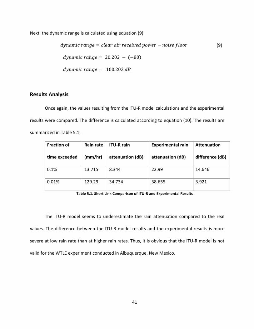
Results Analysis
Once again, the values resulting from the ITU-‐R model calculations and the experimental
results were compared. The difference is calculated according to equation (10). The results are
summarized in Table 5.1.
Fraction of
time exceeded
Rain rate
(mm/hr)
ITU-‐R rain
attenuation (dB)
Experimental rain
attenuation (dB)
Attenuation
difference (dB)
0.1% 13.715 8.344 22.99 14.646
0.01% 129.29 34.734 38.655 3.921
Table 5.1. Short Link Comparison of ITU-‐R and Experimental Results
The ITU-‐R model seems to underestimate the rain attenuation compared to the real
values. The difference between the ITU-‐R model results and the experimental results is more
severe at low rain rate than at higher rain rates. Thus, it is obvious that the ITU-‐R model is not
valid for the WTLE experiment conducted in Albuquerque, New Mexico.
42
Fitting of ITU-‐R Model
The K and a coefficients used in the analysis so far are given by the ITU-‐R model. However,
these coefficients are highly dependent on climate conditions and cannot be assigned one single
value to cover any experiment, independently of the region where the experiment is conducted.
Conversely, the climate regime of the region under consideration should be taken into account
to find the appropriate values of the K and a coefficients to check if the ITU-‐R model can correctly
estimate the experimental signal attenuation. Therefore, in the following section, the least
square error fitting method was used to fit the K and a coefficients in the ITU-‐R model to the
experimental results. As mentioned earlier, the ITU-‐R model uses the rain rate to calculate the
attenuation in dB/Km according to equation (5). Originally, the k and a coefficients given by the
ITU-‐R at 84 GHz are the following:
𝑘 = 1.2164
𝛼 = 0.6999
After fitting the experimental values, it turned out that the corrected k and a coefficients,
with a 95% confidence bounds, that should be used with the ITU-‐R model to calculate the
attenuation for the WTLE link are the following:
𝑘 = 17.5 (17.18, 17.82)
𝛼 = 0.06003 (0.05796, 0.0621)
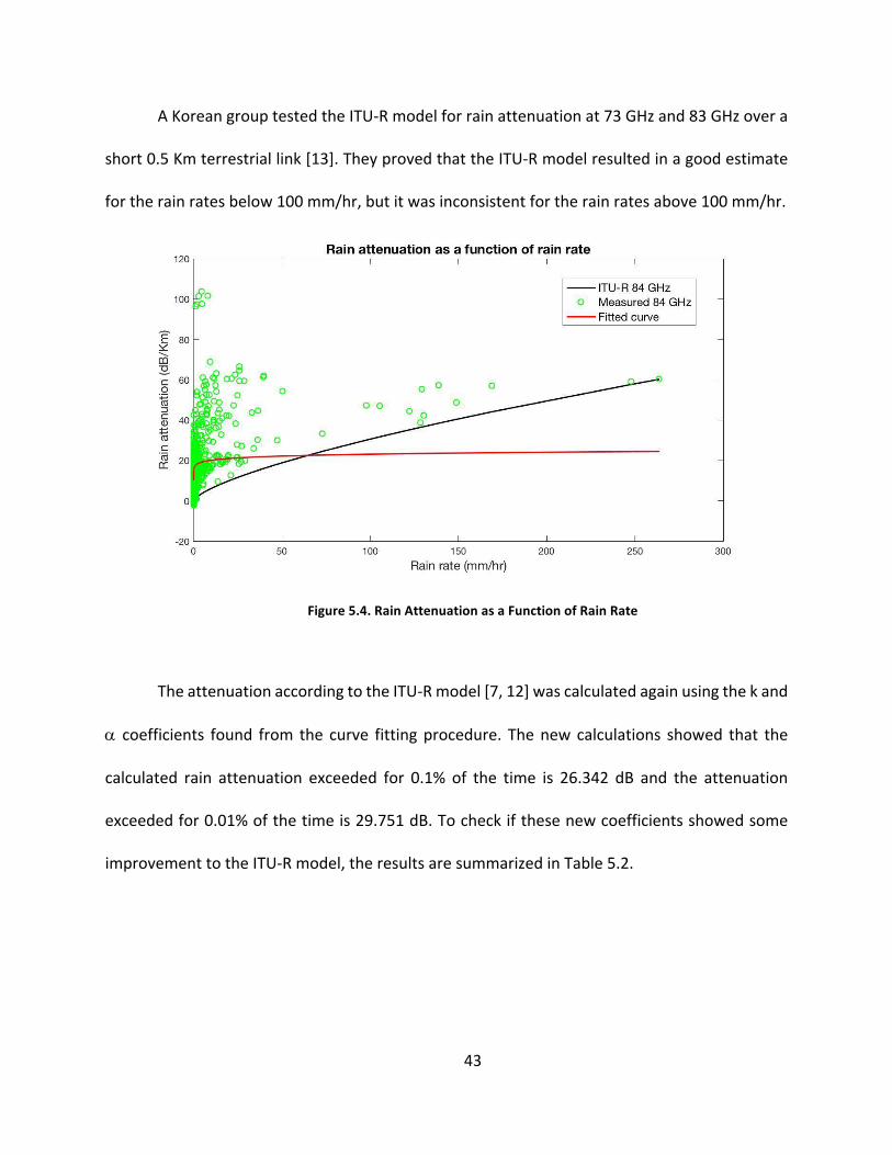
Figure 5.4 shows the measured attenuation as a function of rain rate, the original
calculated attenuation using the k and a coefficients suggested by the ITU-‐R model, and the fitted
attenuation corresponding specifically to the short link experiment.
43
A Korean group tested the ITU-‐R model for rain attenuation at 73 GHz and 83 GHz over a
short 0.5 Km terrestrial link [13]. They proved that the ITU-‐R model resulted in a good estimate
for the rain rates below 100 mm/hr, but it was inconsistent for the rain rates above 100 mm/hr.
Figure 5.4. Rain Attenuation as a Function of Rain Rate
The attenuation according to the ITU-‐R model [7, 12] was calculated again using the k and
a coefficients found from the curve fitting procedure. The new calculations showed that the
calculated rain attenuation exceeded for 0.1% of the time is 26.342 dB and the attenuation
exceeded for 0.01% of the time is 29.751 dB. To check if these new coefficients showed some
improvement to the ITU-‐R model, the results are summarized in Table 5.2.
44
Fraction of time
exceeded
Rain rate
(mm/hr)
Difference with old k
and a (dB)
Difference with new k
and a (dB)
0.1% 13.715 14.646 -‐3.352
0.01% 129.29 3.921 8.904
Table 5.2. Comparison of ITU-‐R Model before fitting and after fitting
When the rain rate was 13.715 mm/hr, at the lower limit of the heavy rain rate category
according to Table 2.3, the fitted curve showed significant improvement in matching the ITU-‐R
model to the experiment compared to the results noted previously when using the original k and
a coefficients values. However, when the rain rate was 129.29 mm/hr, which is categorized as
violent rain rate according to Table 2.3, the fitted curve coefficients resulted in a worse matching
than the one gotten when using the original k and a coefficients with the ITU-‐R model.
Albuquerque is considered to be slightly in the heavy rain rate category, as mentioned in
Chapter 3. Moreover, it is clearly noticeable from Figure 5.4 that the majority of the rain events
occurred between 0 and 25 mm/hr. A larger set of data is needed to validate the following theory,
however as a preliminary finding, the power law relationship 𝛾" = 𝑘𝑅& given by the ITU-‐R to
calculate the rain attenuation cannot be fitted to the real data for the Albuquerque region. A
different equation form having a steeper slope for low rain rates and a slope converging to
saturation at high rain rates must be generated.
45
Chapter 6 – Conclusion
The ITU-‐R model for rain attenuation [7, 12] proved to be invalid for the WTLE experiment.
This model depends highly on the k and a coefficients, that in turn depend on the frequency of
operation and on the rain regime of the region of interest.
Even when trying to fit these coefficients to the experiment using the least square error,
a general result satisfying low rain rates and high rain rates concurrently could not be found. A
new form of the equation might be needed to account for the special climate conditions in
Albuquerque, New Mexico.
The WTLE experiment is an ongoing project, more resources will be added continuously
to help improve the accuracy of the experiment and understand the effects of the weather
conditions on the propagating signal in more depth. Some of the expected improvements in the
future are, adding disdrometers and weather stations at different locations along the path to
have a better understanding of the climate conditions all over the path, and adding a fog sensor
at the transmitter site on top of the Sandia Peak to be able to monitor the clouds effect on the
signal.
46
References
[1] “Millimeter Wave Propagation: Spectrum Management Implications”, Federal
Communications Commission, Bulletin Number 70, July 1997.
[2] Kesavan, U. Tharek, A.R. and Rafiqul Islam M., “Rain Attenuation Prediction Using
Frequency Scaling Technique at Tropical Region for Terrestrial Link”, Progress in
Electromagnetics Research Symposium Proceedings, 2013.
[3] N. Tarasenko, et. al., “W/V-‐Band Terrestrial Link Experiment, an Overview”, IEEE APS/URSI,
2016.
[4] Climate Research Facility, Instruments categories,
https://www.arm.gov/instruments/disdrometer
[5] Next Generation Radar, Nexrad, https://www.wunderground.com/weather-‐radar/united-‐
states/nm/albuquerque/abx/
[6] National Center for Environmental Information, NOAA’s Weather and Climate Toolkit.
https://www.ncdc.noaa.gov/wct/
[7] “Specific Attenuation Model for Rain for Use in Prediction Methods”, ITU-‐R P.838-‐3, 2005.
[8] “Specific Attenuation Model for Rain for Use in Prediction Methods”, ITU-‐ R P .838-‐2, 2003.
[9] Da Silva Mello, L.A.R.; Pontes, M.S.; de Souza, R.M.; Perez Garcia, N.A., “Prediction of rain
attenuation in terrestrial links using full rainfall rate distribution,” in Electronics Letters ,
vol.43, no.25, pp.1442-‐1443, Dec. 6 2007.
[10] Met Office, “Fact Sheet No. 3: Water in the Atmosphere”, Crown Copyright, p. 6, August
2007
47
[11] Albuquerque New Mexico Average Rainfall, Weather DB,
https://rainfall.weatherdb.com/l/165/Albuquerque-‐New-‐Mexico
[12] “Propagation data and prediction methods required for the design of terrestrial line-‐of-‐
sight systems”, ITU-‐R P.530-‐16, 2015.
[13] Kim, J. Jung, M. Yoon, and Y. Chong, Y. “The Measurements of Rain Attenuation for
Terrestrial Link at millimeter Wave”. 2013

48
Appendix A
Matlab Code for the WTLE Link Statistical Analysis
Matlab version: Matlab_R2016a clear all; close all; clc; %---------------------------------------------------------------------------- %Read the attenuation at 72 GHz and 84 GHz from the nids text files and save them in a single column. f=input('Input the frequency of operation 72 or 84 (GHz): '); if f == 72; noisefloor = -75; else noisefloor = -80; end if f == 72; pathstr = '/Users/nadinedaoud/Documents/UNM/Work/Fall 2016/Long Link/72 GHz attenuation nids files'; folder_name=uigetdir(pathstr); files=dir(fullfile(folder_name,'*.txt')); curr_folder=pwd; cd(folder_name); disp(length(files)); for i=1:length(files) fid=fopen(files(i).name,'r'); m = textscan(fid,'%*f %*f %*f %*f %*f %*f %*f %*f %f %*f %*f %*f %*f %*f %*f %*f','delimiter',' ','MultipleDelimsAsOne',1); if i==1 A(:,i)=m{:}; else A = vertcat(A, m); end fclose(fid); end save('attenuation72.mat','A'); else pathstr = '/Users/nadinedaoud/Documents/UNM/Work/Fall 2016/Long Link/84 GHZ attenuation nids files'; folder_name=uigetdir(pathstr); files=dir(fullfile(folder_name,'*.txt')); curr_folder=pwd; cd(folder_name); disp(length(files)); for i=1:length(files) fid=fopen(files(i).name,'r'); m = textscan(fid,'%*f %*f %*f %*f %*f %*f %*f %*f %f %*f %*f %*f %*f %*f %*f %*f','delimiter',' ','MultipleDelimsAsOne',1); if i==1 A(:,i)=m{:};
49
else A = vertcat(A, m); end fclose(fid); end save('attenuation84.mat','A'); end %---------------------------------------------------------------------------- %Save the total attenuation at 72 GHz and 84 GHz in two different columns if f == 72; attenuation72=load('attenuation72.mat'); attenuation72=attenuation72.A; Allattenuation = {cat(1,attenuation72{:})}; Allattenuation = Allattenuation{:}; else attenuation84=load('attenuation84.mat'); attenuation84=attenuation84.A; Allattenuation = {cat(1,attenuation84{:})}; Allattenuation = Allattenuation{:}; end %---------------------------------------------------------------------------- %Read the rain rate for 72 GHz and 84 GHz from the nids text files and save them in a single column. pathstr = '/Users/nadinedaoud/Documents/UNM/Work/Fall 2016/Long Link/Receiver rain rate nids files'; folder_name=uigetdir(pathstr); files=dir(fullfile(folder_name,'*.txt')); curr_folder=pwd; cd(folder_name); disp(length(files)); for i=1:length(files) fid=fopen(files(i).name,'r'); m = textscan(fid,'%*f %f %*f %*f %*f %*f %*f %*f %*f %*f %*f %*f %*f %*f %*f %*f %*f %*f %*f %*f %*f %*f %*f %*f %*f %*f %*f %*f %*f %*f %*f %*f %*f %*f %*s','delimiter',' ','MultipleDelimsAsOne',1); if i==1 B(:,i)=m{:}; else B = vertcat(B, m); end fclose(fid); end save('rain.mat','B'); %---------------------------------------------------------------------------- %Save the rain rate in an array. rain=load('rain.mat'); rain=rain.B; Allrain = {cat(1,rain{:})}; Allrain=Allrain{:}; %---------------------------------------------------------------------------- %Delete all the rain rate values that record a rain rate of 999.999 mm/hr [rows junk] = size (Allrain); for i=1:rows
50
if Allrain(rows-i+1) == 999.999 Allrain(rows-i+1)=[]; end end %Quick exceedance binning exercise %determine the set size setsize=length(Allrain); %exceedance plot resolution res=0.01; %determine the number of power steps ressize=(max(Allrain)-min(Allrain))/res; %initialize empty array for data exceedanceplot_rain=zeros(floor(ressize)+1,2); iterate=0; start=min(Allrain); finish=max(Allrain); %march through the plot while start+ iterate*res <= finish exceedanceplot_rain(iterate+1,:)=[sum(Allrain>=(start+res*iterate))/setsize,start+res*iterate]; iterate=iterate+1; end xrain=exceedanceplot_rain(:,1); yrain=exceedanceplot_rain(:,2); desiredXValue01=0.001; xrain01 = find(abs(xrain-desiredXValue01) < 0.00005); xrain01=xrain01(1:19,:); desiredYValues=yrain(xrain01); rainyDesired_01=mean(desiredYValues); desiredXValue001=0.0001; xrain001 = find(abs(xrain-desiredXValue001) < 0.000001882); xrain001=xrain001(1:58,:); desiredYValues=yrain(xrain001); rainyDesired_001=mean(desiredYValues); %generate the plot fig1=figure; set(fig1,'name','Rain','numbertitle','off') semilogx(xrain,yrain) v=vline(desiredXValue01,'r'); h=hline(rainyDesired_01,'r'); fprintf('\nThe rainfall rate exceeded for 0.1 percent of the time at %i GHz is %f mm/hr',f, rainyDesired_01);
51
v=vline(desiredXValue001,'g'); h=hline(rainyDesired_001,'g'); fprintf('\nThe rainfall rate exceeded for 0.01 percent of the time at %i GHz is %f mm/hr',f, rainyDesired_001); %---------------------------------------------------------------------------- %Calculate the attenuation (dB/km) corresponding to the rainfall rate %exceeded for 0.1% and 0.01% of the time. [rainattenuation_01,alpha,d] = Rainattenuation(rainyDesired_01,f); [rainattenuation_001,alpha,d] = Rainattenuation(rainyDesired_001,f); %---------------------------------------------------------------------------- %Calculate the distance factor r for our link and the effective distance r_01 = 1/((((0.477*(d^0.633))*(rainyDesired_01^(0.073*alpha))*(f^0.123)))-(10.579*(1-exp(-0.024*d)))); deff_01 = r_01*d; r_001 = 1/((((0.477*(d^0.633))*(rainyDesired_001^(0.073*alpha))*(f^0.123)))-(10.579*(1-exp(-0.024*d)))); deff_001 = r_001*d; %---------------------------------------------------------------------------- %Calculate the total attenuation exceeded for 0.1% and 0.01% of the time for the %overall link A_01=rainattenuation_01*deff_01; A_001=rainattenuation_001*deff_001; fprintf('\nThe total calculated attenuation exceeded for 0.1 percent of the time at %i GHz is %f dB',f, A_01); fprintf('\nThe total calculated attenuation exceeded for 0.01 percent of the time at %i GHz is %f dB',f, A_001); %---------------------------------------------------------------------------- %Calculate the total measured attenuation [rows junk] = size (Allattenuation); Allattenuation = Allattenuation(:,1); Allreceivedpowertest = Allattenuation; Allattenuation(Allattenuation<noisefloor) = noisefloor+0.000001; Allattenuation = 0 - Allattenuation; %Quick exceedance binning exercise %determine the set size setsize=length(Allattenuation); %exceedance plot resolution res=0.01; %determine the number of power steps
52
ressize=(max(Allattenuation)-min(Allattenuation))/res; %initialize empty array for data arraysize=floor(ressize)+1; exceedanceplot_atten=zeros(arraysize,2); iterate=0; start=min(Allattenuation); finish=max(Allattenuation); residual=0; data=Allattenuation; h=waitbar(0,'calculating'); while start+ iterate*res <= finish mask=data>=(start+res*iterate); data=data(mask); exceedanceplot_atten(iterate+1,:)=[sum(mask)/setsize,start+res*iterate]; waitbar((iterate*res+start)/finish) iterate=iterate+1; end close(h) xatten=exceedanceplot_atten(:,1); yatten=exceedanceplot_atten(:,2); if f ==72 desiredXValue01=0.001; xatten01 = find(abs(xatten-desiredXValue01) < 0.005); attenyDesired_01=75; desiredXValue001=0.0001; attenyDesired_001=75; desiredXValue90 = 0.90; xatten90 = find(abs(xatten-desiredXValue90) < 0.002); attenyDesired_90=yatten(xatten90); else desiredXValue01=0.001; xatten01 = find(abs(xatten-desiredXValue01) < 0.0005); % xatten01=xatten01(407:478,:); % desiredYValues=yatten(xatten01); attenyDesired_01=80; desiredXValue001=0.0001; attenyDesired_001=80; desiredXValue90 = 0.90; xatten90 = find(abs(xatten-desiredXValue90) < 0.002); attenyDesired_90=yatten(xatten90); end
53
%generate the plot fig2=figure; set(fig2,'name','Attenuation','numbertitle','off') semilogx(xatten,yatten) v=vline(desiredXValue01,'r'); h=hline(attenyDesired_01,'r'); fprintf('\nThe attenuation exceeded for 0.1 percent of the time at %i GHz is %f dB',f, attenyDesired_01); v=vline(desiredXValue001,'g'); h=hline(attenyDesired_001,'g'); fprintf('\nThe attenuation exceeded for 0.01 percent of the time at %i GHz is %f dB',f, attenyDesired_001); v=vline(desiredXValue90,'k'); h=hline(attenyDesired_90,'k'); fprintf('\nThe clear air attenuation at %i GHz is %f dB',f, attenyDesired_90); rainattenuation01 = attenyDesired_01-attenyDesired_90; fprintf('\nThe rain attenuation relative to clear air exceeded for 0.1 percent of the time at %i GHz is %f dB',f, rainattenuation01); rainattenuation001 = attenyDesired_001-attenyDesired_90; fprintf('\nThe rain attenuation relative to clear air exceeded for 0.01 percent of the time at %i GHz is %f dB',f, rainattenuation001); dynamicrange = attenyDesired_90-noisefloor; fprintf('\nThe dynamic range for this rain event at %i GHz is %f dB',f, dynamicrange);
54
Appendix B
Matlab Code for the Short Link Statistical Analysis
Matlab version: Matlab_R2016a clear all; close all; clc; f=84; noisefloor = -80; %---------------------------------------------------------------------------- %Read the attenuation at 84 GHz from the nids text files and save them in a single column. pathstr = '/Users/nadinedaoud/Documents/UNM/Work/Fall 2016/Short Link/NEW_20161004/84GHz nids files'; folder_name=uigetdir(pathstr); files=dir(fullfile(folder_name,'*.txt')); curr_folder=pwd; cd(folder_name); disp(length(files)); for i=1:length(files) fid=fopen(files(i).name,'r'); m = textscan(fid,'%*f %*f %*f %*f %*f %*f %*f %*f %f %*f %*f %*f %*f %*f %*f %*f','delimiter',' ','MultipleDelimsAsOne',1); if i==1 A(:,i)=m{:}; else A = vertcat(A, m); end fclose(fid); end save('attenuation84.mat','A'); %---------------------------------------------------------------------------- %Save the total attenuation at 84 GHz in a single column attenuation84=load('attenuation84.mat'); attenuation84=attenuation84.A; Allattenuation = {cat(1,attenuation84{:})}; Allattenuation = Allattenuation{:}; %---------------------------------------------------------------------------- %Read the rain rate for 84 GHz from the nids text files and save them in a single column. pathstr = '/Users/nadinedaoud/Documents/UNM/Work/Fall 2016/Short Link/NEW_20161004/Receiver rain rate nids files'; folder_name=uigetdir(pathstr); files=dir(fullfile(folder_name,'*.txt')); curr_folder=pwd; cd(folder_name);
55
disp(length(files)); for i=1:length(files) fid=fopen(files(i).name,'r'); m = textscan(fid,'%*f %f %*f %*f %*f %*f %*f %*f %*f %*f %*f %*f %*f %*f %*f %*f %*f %*f %*f %*f %*f %*f %*f %*f %*f %*f %*f %*f %*f %*f %*f %*f %*f %*f %*s','delimiter',' ','MultipleDelimsAsOne',1); if i==1 B(:,i)=m{:}; else B = vertcat(B, m); end fclose(fid); end save('rain.mat','B'); %---------------------------------------------------------------------------- %Save the rain rate in an array. rain=load('rain.mat'); rain=rain.B; Allrain = {cat(1,rain{:})}; Allrain=Allrain{:}; %---------------------------------------------------------------------------- %Delete all the files when we have missing data during the day C = [A B]; [rows junk] = size (C); for i=1:rows [Arows junk] = cellfun(@size,A,'uni',false); end for i=1:rows if Arows{rows-i+1} ~= 86400; C(rows-i+1,:)=[]; end end D=C; [rows junk] = size (D); for i=1:rows shortB{i,1} = D{i,2}; end for i=1:rows [Brows junk] = cellfun(@size,shortB,'uni',false); end for i=1:rows if Brows{rows-i+1} ~= 1440; C(rows-i+1,:)=[]; end end AA = {cat(1,C{:,1})}; AA=AA{:}; BB = {cat(1,C{:,2})}; BB=BB{:}; %---------------------------------------------------------------------------- %Calculate the mean of each 60 consecutive rows (because every 60 seconds are equal to 1 minute. %Then store the resultant means in an array. %I am interested in every 1 min data not every 1 second data to be able to %assign every 1 min received power to every 1 min rain rate.
56
[rows junk]=size(AA); lastelement=60*floor(rows/60); indices= lastelement+1:rows; AA(indices,:)=[]; meanAA = mean(reshape(AA,60,[])); meanAA=transpose(meanAA); CC=[meanAA BB]; %---------------------------------------------------------------------------- %Delete all the rain rate values that record a rain rate of 999.999 mm/hr [rows junk] = size (Allrain); for i=1:rows if Allrain(rows-i+1) == 999.999 Allrain(rows-i+1)=[]; end end %Quick exceedance binning exercise %determine the set size setsize=length(Allrain); %exceedance plot resolution res=0.01; %determine the number of power steps ressize=(max(Allrain)-min(Allrain))/res; %initialize empty array for data exceedanceplot_rain=zeros(floor(ressize)+1,2); iterate=0; start=min(Allrain); finish=max(Allrain); %march through the plot while start+ iterate*res <= finish exceedanceplot_rain(iterate+1,:)=[sum(Allrain>=(start+res*iterate))/setsize,start+res*iterate]; iterate=iterate+1; end xrain=exceedanceplot_rain(:,1); yrain=exceedanceplot_rain(:,2); desiredXValue01=0.001; xrain01 = find(abs(xrain-desiredXValue01) < 0.00005); xrain01=xrain01(1:162,:); desiredYValues=yrain(xrain01); rainyDesired_01=mean(desiredYValues); desiredXValue001=0.0001; xrain001 = find(abs(xrain-desiredXValue001) < 0.000002); xrain001=xrain001(98,:);
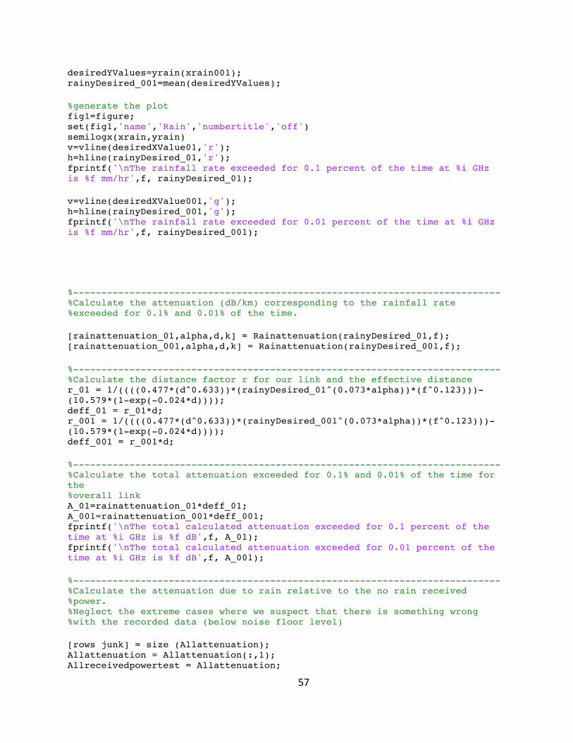
57
desiredYValues=yrain(xrain001); rainyDesired_001=mean(desiredYValues); %generate the plot fig1=figure; set(fig1,'name','Rain','numbertitle','off') semilogx(xrain,yrain) v=vline(desiredXValue01,'r'); h=hline(rainyDesired_01,'r'); fprintf('\nThe rainfall rate exceeded for 0.1 percent of the time at %i GHz is %f mm/hr',f, rainyDesired_01); v=vline(desiredXValue001,'g'); h=hline(rainyDesired_001,'g'); fprintf('\nThe rainfall rate exceeded for 0.01 percent of the time at %i GHz is %f mm/hr',f, rainyDesired_001); %---------------------------------------------------------------------------- %Calculate the attenuation (dB/km) corresponding to the rainfall rate %exceeded for 0.1% and 0.01% of the time. [rainattenuation_01,alpha,d,k] = Rainattenuation(rainyDesired_01,f); [rainattenuation_001,alpha,d,k] = Rainattenuation(rainyDesired_001,f); %---------------------------------------------------------------------------- %Calculate the distance factor r for our link and the effective distance r_01 = 1/((((0.477*(d^0.633))*(rainyDesired_01^(0.073*alpha))*(f^0.123)))-(10.579*(1-exp(-0.024*d)))); deff_01 = r_01*d; r_001 = 1/((((0.477*(d^0.633))*(rainyDesired_001^(0.073*alpha))*(f^0.123)))-(10.579*(1-exp(-0.024*d)))); deff_001 = r_001*d; %---------------------------------------------------------------------------- %Calculate the total attenuation exceeded for 0.1% and 0.01% of the time for the %overall link A_01=rainattenuation_01*deff_01; A_001=rainattenuation_001*deff_001; fprintf('\nThe total calculated attenuation exceeded for 0.1 percent of the time at %i GHz is %f dB',f, A_01); fprintf('\nThe total calculated attenuation exceeded for 0.01 percent of the time at %i GHz is %f dB',f, A_001); %---------------------------------------------------------------------------- %Calculate the attenuation due to rain relative to the no rain received %power. %Neglect the extreme cases where we suspect that there is something wrong %with the recorded data (below noise floor level) [rows junk] = size (Allattenuation); Allattenuation = Allattenuation(:,1); Allreceivedpowertest = Allattenuation;
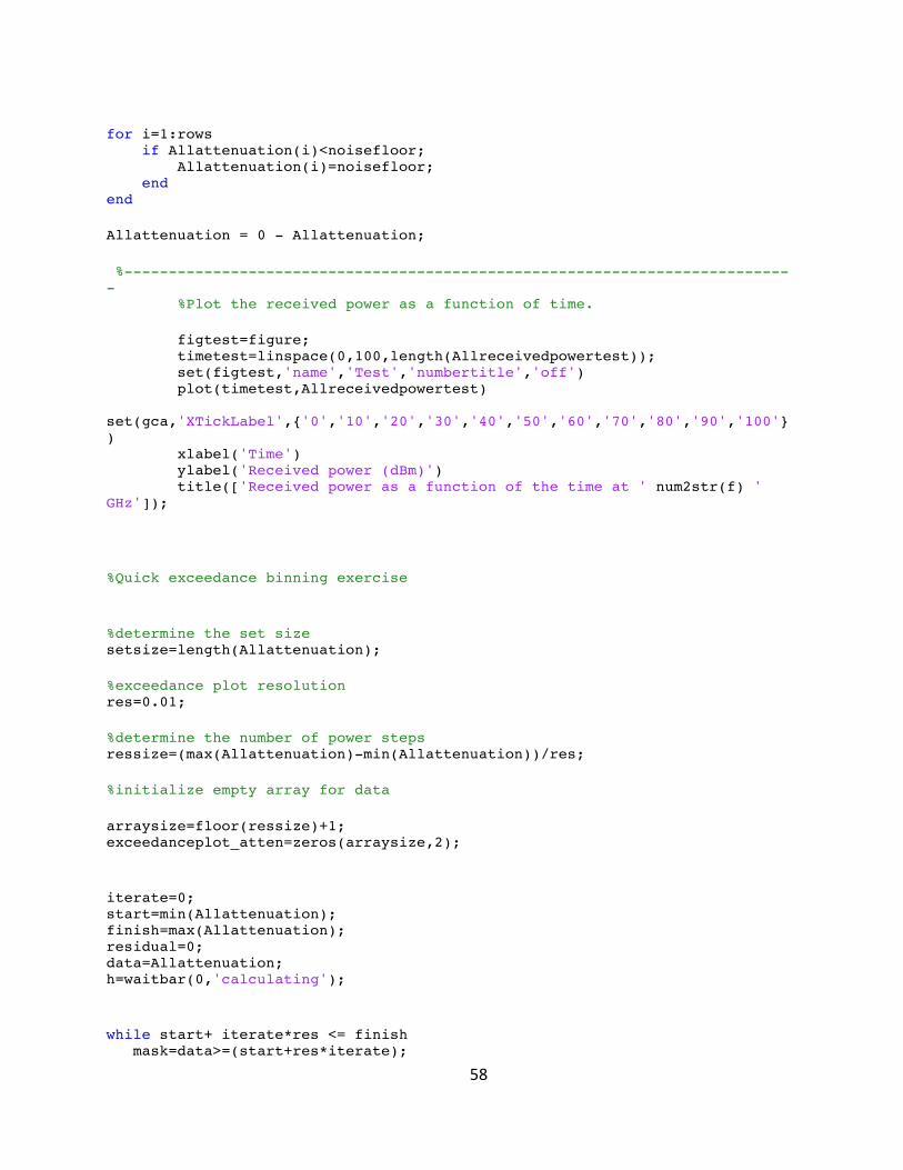
58
for i=1:rows if Allattenuation(i)<noisefloor; Allattenuation(i)=noisefloor; end end Allattenuation = 0 - Allattenuation; %---------------------------------------------------------------------------- %Plot the received power as a function of time. figtest=figure; timetest=linspace(0,100,length(Allreceivedpowertest)); set(figtest,'name','Test','numbertitle','off') plot(timetest,Allreceivedpowertest) set(gca,'XTickLabel',{'0','10','20','30','40','50','60','70','80','90','100'}) xlabel('Time') ylabel('Received power (dBm)') title(['Received power as a function of the time at ' num2str(f) ' GHz']); %Quick exceedance binning exercise %determine the set size setsize=length(Allattenuation); %exceedance plot resolution res=0.01; %determine the number of power steps ressize=(max(Allattenuation)-min(Allattenuation))/res; %initialize empty array for data arraysize=floor(ressize)+1; exceedanceplot_atten=zeros(arraysize,2); iterate=0; start=min(Allattenuation); finish=max(Allattenuation); residual=0; data=Allattenuation; h=waitbar(0,'calculating'); while start+ iterate*res <= finish mask=data>=(start+res*iterate);
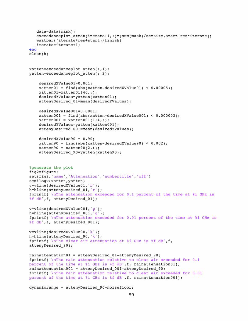
59
data=data(mask); exceedanceplot_atten(iterate+1,:)=[sum(mask)/setsize,start+res*iterate]; waitbar((iterate*res+start)/finish) iterate=iterate+1; end close(h) xatten=exceedanceplot_atten(:,1); yatten=exceedanceplot_atten(:,2); desiredXValue01=0.001; xatten01 = find(abs(xatten-desiredXValue01) < 0.00005); xatten01=xatten01(40,:); desiredYValues=yatten(xatten01); attenyDesired_01=mean(desiredYValues); desiredXValue001=0.0001; xatten001 = find(abs(xatten-desiredXValue001) < 0.000003); xatten001 = xatten001(1:4,:); desiredYValues=yatten(xatten001); attenyDesired_001=mean(desiredYValues); desiredXValue90 = 0.90; xatten90 = find(abs(xatten-desiredXValue90) < 0.002); xatten90 = xatten90(2,:); attenyDesired_90=yatten(xatten90); %generate the plot fig2=figure; set(fig2,'name','Attenuation','numbertitle','off') semilogx(xatten,yatten) v=vline(desiredXValue01,'r'); h=hline(attenyDesired_01,'r'); fprintf('\nThe attenuation exceeded for 0.1 percent of the time at %i GHz is %f dB',f, attenyDesired_01); v=vline(desiredXValue001,'g'); h=hline(attenyDesired_001,'g'); fprintf('\nThe attenuation exceeded for 0.01 percent of the time at %i GHz is %f dB',f, attenyDesired_001); v=vline(desiredXValue90,'k'); h=hline(attenyDesired_90,'k'); fprintf('\nThe clear air attenuation at %i GHz is %f dB',f, attenyDesired_90); rainattenuation01 = attenyDesired_01-attenyDesired_90; fprintf('\nThe rain attenuation relative to clear air exceeded for 0.1 percent of the time at %i GHz is %f dB',f, rainattenuation01); rainattenuation001 = attenyDesired_001-attenyDesired_90; fprintf('\nThe rain attenuation relative to clear air exceeded for 0.01 percent of the time at %i GHz is %f dB',f, rainattenuation001); dynamicrange = attenyDesired_90-noisefloor;
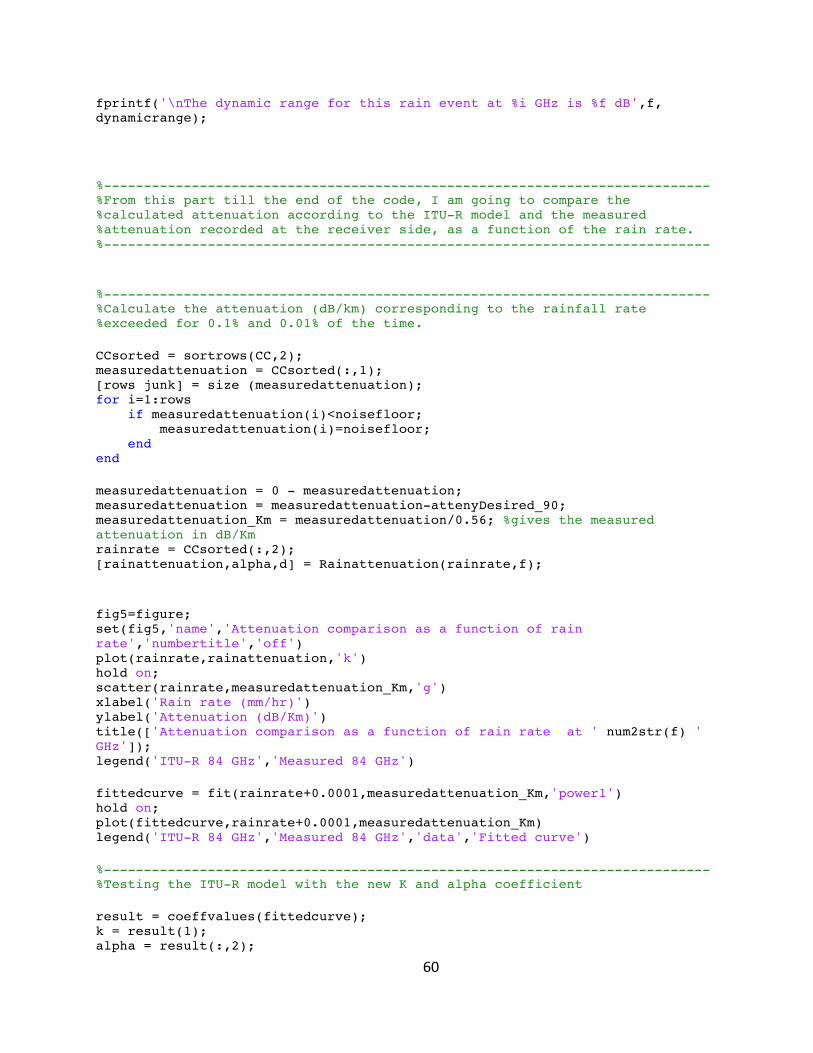
60
fprintf('\nThe dynamic range for this rain event at %i GHz is %f dB',f, dynamicrange); %---------------------------------------------------------------------------- %From this part till the end of the code, I am going to compare the %calculated attenuation according to the ITU-R model and the measured %attenuation recorded at the receiver side, as a function of the rain rate. %---------------------------------------------------------------------------- %---------------------------------------------------------------------------- %Calculate the attenuation (dB/km) corresponding to the rainfall rate %exceeded for 0.1% and 0.01% of the time. CCsorted = sortrows(CC,2); measuredattenuation = CCsorted(:,1); [rows junk] = size (measuredattenuation); for i=1:rows if measuredattenuation(i)<noisefloor; measuredattenuation(i)=noisefloor; end end measuredattenuation = 0 - measuredattenuation; measuredattenuation = measuredattenuation-attenyDesired_90; measuredattenuation_Km = measuredattenuation/0.56; %gives the measured attenuation in dB/Km rainrate = CCsorted(:,2); [rainattenuation,alpha,d] = Rainattenuation(rainrate,f); fig5=figure; set(fig5,'name','Attenuation comparison as a function of rain rate','numbertitle','off') plot(rainrate,rainattenuation,'k') hold on; scatter(rainrate,measuredattenuation_Km,'g') xlabel('Rain rate (mm/hr)') ylabel('Attenuation (dB/Km)') title(['Attenuation comparison as a function of rain rate at ' num2str(f) ' GHz']); legend('ITU-R 84 GHz','Measured 84 GHz') fittedcurve = fit(rainrate+0.0001,measuredattenuation_Km,'power1') hold on; plot(fittedcurve,rainrate+0.0001,measuredattenuation_Km) legend('ITU-R 84 GHz','Measured 84 GHz','data','Fitted curve') %---------------------------------------------------------------------------- %Testing the ITU-R model with the new K and alpha coefficient result = coeffvalues(fittedcurve); k = result(1); alpha = result(:,2);

61
[NEWrainattenuation_01,d] = RainattenuationAlphaK(rainyDesired_01,f,alpha,k); [NEWrainattenuation_001,d] = RainattenuationAlphaK(rainyDesired_001,f,alpha,k); r_01 = 1/((((0.477*(d^0.633))*(rainyDesired_01^(0.073*alpha))*(f^0.123)))-(10.579*(1-exp(-0.024*d)))); deff_01 = r_01*d; r_001 = 1/((((0.477*(d^0.633))*(rainyDesired_001^(0.073*alpha))*(f^0.123)))-(10.579*(1-exp(-0.024*d)))); deff_001 = r_001*d; A_01=NEWrainattenuation_01*deff_01; A_001=NEWrainattenuation_001*deff_001; fprintf('\nThe NEW total calculated attenuation exceeded for 0.1 percent of the time at %i GHz is %f dB',f, A_01); fprintf('\nThe NEW total calculated attenuation exceeded for 0.01 percent of the time at %i GHz is %f dB',f, A_001);