3 Small Subgraphs

3.1 THE CONTAINMENT PROBLEM

In 1960 Erdös and Rényi published the most fundamental of their random graphs papers (Erdös and Rényi 1960). The first problem studied there was that of the existence in G(n, M) of at least one copy of a given graph G. Since the graph G is fixed and the random graph G(n, M) grows with n -► oo, copies of G in G(n, M) are called small subgraphs, regardless whether G is a triangle or a graph with one billion vertices, as opposed to subgraphs of G(n, M) which grow with n like, say, a Hamilton cycle.

Erdös and Rényi (1960) found the threshold for the property of containing G only in the special case in which G is a balanced graph (see Section 3.2 for the definition). Twenty-one years later Bollobás (1981b) settled the problem in full generality. Still later a simpler proof was found by Rucinski and Vince (1985) and we will present it here. It is a classical example of an application of the commonly used methods of the first and the second moment. This problem is also instructive in that it shows that the behavior of the expectation alone can be sometimes misleading.

To better comprehend this feature and to have a gentle start, we will con-sider first the somewhat simpler problem of finding the threshold for the containment of at least one arithmetic progression of length k in a random subset of integers [n]p, where, recall, [n] = {1 ,2 , . . . ,n} and p = p(n) is the probability of including each element of [n], independently of the others, in the random subset [n]p.

53

Random Graphs by Svante Janson, Tomasz Luczak and Andrzej Rucinski

Copyright © 2000 John Wiley & Sons, Inc.

54 SMALL SUBGRAPHS

The first and second moment methods

Before presenting the applications, let us describe the first and the second moment methods. As a special instance of the Markov inequality (1.3), for every non-negative, integer valued random variable X, the inequality

P ( X > 0 ) < E X (3.1)

holds. The first moment method relies on showing that EX n — o(l), and thus concluding by (3.1) that Xn = 0 o.o.s. The second moment method is based on Chebyshev's inequality (1.2), which implies (Exercise!) that for every random variable X with E X > 0

VarX (EX)2 P(*=0><7FVvF· (3·2)

Hence, by showing that the right-hand side of (3.2) (with X replaced by Xn) converges to 0, one concludes that X„ > 0 a.a.s. By the same token one obtains a stronger statement, which also follows from Chebyshev's inequal-ity: If VarXn/(EX„)2 = o(l) then Xn = EX„ + op(EX„) or, equivalently, X„ /EX n A 1. In particular then, Xn = ©c(EX„).

Remark 3.1. Inequality (3.2) may be improved. The Cauchy-Schwarz in-equality applied to X = X1[X Φ 0] yields (EX)2 < EX 2P(X Φ 0), that is,

P(X ¿0)> ^ | | £ , (3.3)

and thus

T(X 0 1 - 1 iEX)2 V a r * V a r * (34) P ( X _ 0 ) < 1 Ε χ 2 - Ε χ 2 - ( E X ) 2 + V a r X · (dA)

For the purpose of showing X„ > 0 o.o.s., (3.2) is just as good as the improve-ment (3.4), but in Chapter 7 we will see a situation where the improvement is essential.

Example 3.2 (arithmetic progressions). Let X* be the number of arith-metic progressions of length k in [n]p, where k > 2 is a fixed integer. (We suppress the subscript n here.) To compute E(X*) we need to know the num-ber /(n,fc) of all arithmetic progressions of length k in [n]. In fact, we only care about the order of magnitude of f(n,k) which equals n2, since every arithmetic progression is uniquely determined by its first two elements. Let us number the arithmetic progressions of length k in [n] by 1 , . . . , /(n, k) and, for each i = l,...,f(n,k), define a zero-one random variable (indicator) U equal to 1 if the i-th arithmetic progression of length k is entirely present in

THE CONTAINMENT PROBLEM 55

[n)p and equal to 0 otherwise. With this notation, Xk = £ ;_" ' »̂ aní*> by the linearity of expectation,

E(Xk) = f(n,k)pk = e(n2pk).

Hence, if p < n _ 2 / * then E{Xk) -> 0 as n -4 oo and, by the first moment method, (i.e. by (3.1)), P(Xk > 0) = o(l).

If, on the other hand, p !» n~2 /*, then E{Xk) -»· oo, but this fact alone is not sufficient to claim that F(Xk > 0) -»· 1. One has to work for it, using the second moment method. Observe that U and / , are independent if the i-th and j - t h arithmetic progressions have no element in common; in that case the covariance Cov(/¿, / , ) equals zero. In the remaining cases, we use the inequality Cov(/¿,/j) < E(J¿Jj). There are 0(n3) pairs (/,,/>) which share one element and then E(/¿Jj) = p 2 * - 1 , and only 0{ri2) pairs which share two or more elements, in which case E(/j/,-) < p*. We thus can estimate the variance of Xk as follows:

/(n.fc) /(n,fc) Varpf*) = Σ Σ Covt/i . / i) = 0(n3p2k~l +n2pk).

Consequently, by the second moment method, (i.e., by (3.2)), if p » n - 2 / * , then

r(xk = o) = o (— + - l j ) = o(i). \np n2pk)

Together, these results show that the threshold for existence of a fc-term arith-metic progression in [n]p is n~2lk.

Thresholds for subgraph containment

Returning to small subgraphs of random graphs, we let XQ stand for the number of copies of a given graph G that can be found in the binomial random graph G(n,p). Let v = VQ and e = eo stand for the number of vertices and edges of G, respectively. There are exactly f{n,G) = (")v!/aut(G) copies of G in the complete graph Kn, where, recall, aut(G) denotes the number of automorphisms of G. For each copy G' of G in Kn define the indicator random variable I& = l[G(n,p) D G']. Then

E(XG) = f(n,G)p< = 0 ( n V ) -> ( ° !Í 1 co if

p<£n-v'e

p^>n-v'e

and, by the first moment method,

P(XG > 0) = o(l) if p « n-v/e. (3.5)

Is it then true that V(XG > 0) = 1 - o(l) if p » n - ^ e ? Consider first an example.

56 SMALL SUBGRAPHS

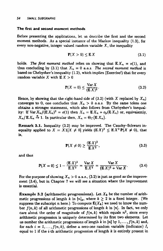
Example 3.3. Let H0 be the graph with 4 vertices and 5 edges and let Go be a graph obtained by adding one vertex to i/o and connecting it to just one vertex of i/o- (There are two nonisomorphic ways to do so, and it does not matter which one we choose - see Figure 3.1 for one version of Go·) Take any sequence p = p(n) such that n - 5 / 6 < p « n _ 4 / 5 , say, p = n _ 9 ^ u . Then EXo0 — Θ{η5ρ6) -> oo, but by (3.5) applied to Ho, a.a.s. there is no copy of Ho in G(n,p), and therefore there is no copy of Go either.

Hence, things are more complicated for graphs than for arithmetic progres-sions. It should be clear at this point that the behavior of the expectation is deceptive in case of Go, because Go contains a subgraph (viz. Ho) denser than itself, and that the right threshold should be n - 4 / 5 . Indeed, this was confirmed by Bollobás (1981b) in the following, general result.

Recall that m(G) is the ratio of the number of edges to the number of vertices in the densest subgraph of G, that is,

m ( G ) = max { — : H C G, vH > θ | . (3.6)

Theorem 3.4. For an arbitrary graph G with at least one edge,

= i° ifl \ l ifl

lim P(Gín,p) D G ) = IP * _ 1 / m ( G ) '

Proof. There are two statements to be proved, the O-statement, and the 1-statement. To prove the former one, assume that p 4C n'1!™^ and let H' be a subgraph of G for which e(H')/v(H') = m(G). Then, by (3.5), o.o.s. there is no copy of H' , and thus, no copy of G in G(n,p).

To prove the 1-statement we use the second moment method; we then need to bound the variance of Xa from above. For future reference, we state the result as a lemma. We define

Φσ = Φσ(η,ρ) = min{E(X//) : H C G, eH > 0} (3.7)

and note that

Φ σ χ min n » V ; (3-8) HCG,CH>0

this quantity will be useful on several occasions in the sequel.

L e m m a 3.5. Let G be a graph vAth at least one edge. Then

Var(XG)x(l-p) £ n2va-vHp2e0-eH

HCG,eH>0

x ( l - p ) max _ , ' = (1 - p ) — , (3.9) V y'HCG,r„>0 EXH Φθ

THE CONTAINMENT PROBLEM 57

where the implicit constants depend on G but not on n or p. In particular, VarXa = 0({EXG)2/$G), and if p - p(n) is bounded away from 1, then VarXG - ( E X G ) 2 / * C

Proof. Using the fact that IG· and IG·· are independent if E{G')C\E{G") = 0, and that for each H CG there are Θ(ην"η21ν°-υ»ϊ) - Q(n^o-vH) p a i r s (G',G") of copies of G in the complete graph Kn with G' Π G" isomorphic to H, we have

Var(XG) = Σ Cav(Ia·, ¡a··) = Σ ^ ' / G " > " E < / G ' > E ( / G " M G',G" E(G')n£(G")/0

x Σ n2 t , c-"H(p2<,c_eH - p 2 e ° ) « C G , Í H > 0

x Σ n2v°-VHf?ea-'-(\-p). (3.10) HCG,eH>0

The simple observation below is often useful.

Lemma 3.6. The following are equivalent, for any graph G with eG > 0.

(i) npm<G) -¥ oo.

(ii) nv"pe" -> oo /or every H CG with VH > 0.

(iii) E(XH) -*■ oo for every H CG with vH > 0.

(iv) φ σ -> oo.

Proo/. By (3.6) (and p < 1), (i) holds if and only if npe"lv" -> oo for every H CG with υ// > 0; since

E X „ x nv"pe" = {npe«lv")VH,

this is equivalent to both (ii) and (iii). Finally, by the definition (3.7), Con-dition (iv) is equivalent to E{XH) -> oo for every H CG with e# > 0; this is equivalent to (iii) since the case VH > 0 and e« = 0 is trivial. ■

To complete the proof of Theorem 3.4, we observe that if p » n_ l /m^G ' , then by Lemma 3.6 Φσ -*· oo. Consequently, (3.2) and Lemma 3.5 yield

P(G(n,p) 2 G) = F(XG = 0) < l ^ f f i = 0(1/Φσ) = o(l). ■

Remark 3.7. It follows from the above proof that if Φσ(η,ρ) -> oo, then not only P(G(n,p) # G) -> 1 but further XG/E(A"G) A 1.

58 SMALL SUBGRAPHS

Go F0

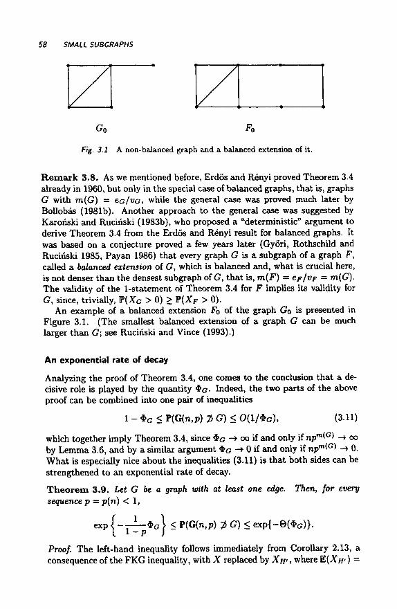
Fig. 3.1 A non-balanced graph and a balanced extension of it.

Remark 3.8. As we mentioned before, Erdös and Rényi proved Theorem 3.4 already in 1960, but only in the special case of balanced graphs, that is, graphs G with m(G) = ec/vG, while the general case was proved much later by Bollobás (1981b). Another approach to the general case was suggested by Karonski and Rucinski (1983b), who proposed a "deterministic" argument to derive Theorem 3.4 from the Erdös and Rényi result for balanced graphs. It was based on a conjecture proved a few years later (Gyori, Rothschild and Rucinski 1985, Payan 1986) that every graph G is a subgraph of a graph F, called a balanced extension of G, which is balanced and, what is crucial here, is not denser than the densest subgraph of G, that is, m(F) = ep/vF = m(G). The validity of the l-statement of Theorem 3.4 for F implies its validity for G, since, trivially, F{XG > 0) > V(XF > 0).

An example of a balanced extension F0 of the graph Go is presented in Figure 3.1. (The smallest balanced extension of a graph G can be much larger than G; see Rucinski and Vince (1993).)

An exponential rate of decay

Analyzing the proof of Theorem 3.4, one comes to the conclusion that a de-cisive role is played by the quantity Φβ· Indeed, the two parts of the above proof can be combined into one pair of inequalities

1 - Φ σ < P(G(n,p) 25 G) < 0 ( 1 / Φ σ ) , (3.11)

which together imply Theorem 3.4, since Φ σ -» oo if and only if npm<-G) -+ oo by Lemma 3.6, and by a similar argument Φβ -ν 0 if and only if npm<>C) -» 0. What is especially nice about the inequalities (3.11) is that both sides can be strengthened to an exponential rate of decay.

Theorem 3.9. Let G be a graph with at least one edge. Then, for every sequence p = p(n) < 1,

exp j - γ - ^ — Φ σ | < P(G(n,p) 0 G) < β χ ρ { - θ ( Φ σ ) } .

Proof. The left-hand inequality follows immediately from Corollary 2.13, a consequence of the FKG inequality, with X replaced by Xw, where E(X«-) =

THE CONTAINMENT PROBLEM 59

Φο- The other inequality is implied by Theorem 2.18(ii) with S = XG and the /yi's replaced by /G 'S . Indeed, the denominator of the exponent there becomes

Σ Σ Σ P2ec"e"=e((EA'c.)V*G) (3.12) HCG,eH>0 G' G"nG'=H

and the right-hand inequality in Theorem 3.9 follows. ■

Note that Theorem 3.9 implies Theorem 3.4.

Remark 3.10 (Martingale approach). There are at least two other ways to deduce the right-hand inequality of Theorem 3.9; they are based, respec-tively, on the martingale and Talagrand inequalities given in Chapter 2. Here we present the martingale approach and the other one will be given in Sec-tion 3.5.

We confine ourselves to the special case in which for every proper subgraph H of G with eH > 0, E(XH) » * σ · In particular, Φ σ = E{XG)- (The general case is quite involved and we refer the reader to Janson, Luczak and Rucinski (1990).) Let / = οΦσ for a suitably chosen constant c > 0, and let π = ( A i , . . . , A/) be an arbitrary partition of the set [n]2 into sets of size | A¿| < n 2 / / , i = 1 , . . . , / . Two copies of G are called π-disjoint if for each index i at most one of them has an edge in Aj. Let D „ G be the maximum number of π-disjoint copies of G in G(n,p). Then, by Corollary 2.27,

P(XG = 0) = P ( D , t 0 = 0) < Ρ(|2?.,σ - t\ > t) < 2 e x p { - i 2 / 2 / } ,

where t = E(Dn<a) < $ σ · Now we need to bound t from below. Let YV¡G be the number of ηοη-π-disjoint pairs of copies of G. Clearly, D„,G > XG - Yn.G, and so t > Φα — E(Y*,G)- When computing E(Y„,G) asymptotically, we may ignore all pairs of G sharing at least one edge, as their expectation is ο(Φσ). The expected number of the other ηοη-π-disjoint pairs is

° (f(n22f)n2{VO~2)P2e°) = °<*o//>· Hence, for sufficiently large c, t = Ω(Φσ) and the right-hand inequality of Theorem 3.9 follows.

The uniform model G(n, M )

In this section we consider the containment problem for the uniform ran-dom graph G(n,M). We note first that by Corollary 1.16 (or Remark 1.18), Theorem 3.4 immediately implies the corresponding result for G(n, M): the threshold is n 2 - 1 /m (G>. (This can also be shown directly by the first and second moment methods.)

For the exponential bounds in Theorem 3.9, the situation is somewhat more complicated. Not only do neither part of the proof of Theorem 3.9 carry

60 SMALL SUBGRAPHS

over to G(n, M), but the result cannot be true in general. Indeed, for dense graphs Turin's theorem (see, e.g., Bollobás (1998)) shows, for example, that if G = Kz and M > \n2 ~ 5(2), then G(n, M) always contains a copy of G, so P(G(n, M) ~fi G) = 0. More generally, by the Erdös-Stone-Simonovits Theorem (Erdös and Stone 1946, Erdös and Simonovits 1966, Diestel 1996, Bollobás 1998), the same holds for any graph G and for M > c("), provided c > 1 - l / (x(G) - 1) is fixed and n is large enough. However, if M is not too large, both inequalities in Theorem 3.9 have counterparts for G(n, M).

For a sequence M = M(n) < (!}), define Φα by (3.7) with p = Μ / β ) , and note that (if G is non-empty) Φ σ < E(X K j ) = {"2)p = M.

T h e o r e m 3.11. Let G be a graph with at least one edge.

(i) / / M >eG, then

P(G(n,M) ¡Z5 G) < ε χ ρ { - θ ( Φ σ ) } .

(ii) //, in addition, either Φο < °M', where c is some small positive constant depending on G, or G is not bipartite and M < c("), where c < 1 — 1/(X(G) - 1) is fixed, then

P(G(n,M) 0 G) = exp{-Q(<bG)}.

Proof. We will give several arguments which are valid for different ranges of M and together yield the results. We let ci ,c2 , - . . denote some positive constants depending on G only. Note that we may assume that n is large, since the results are trivial for any finite number of small n. (i) For Φσ 3> logn, the estimate in (i) follows immediately from the upper bound in Theorem 3.9 and Pittel's inequality (1.6).

Alternatively and more generally, we find by monotonicity and the law of total probability, as in (1.5),

P(G(n,p/2) DG)< P(G(n, M) D G) + P(e(G(n,p/2)) > M)

and thus, using the Chernoff bound (2.7) (or (2.5)), Theorem 3.9 and the fact that Φσ(η,ρ/2) > 2_ < ! ( σ )Φσ(η,ρ), we get

P(G(n,M) 75 G) < P(G(n,p/2) 2 G) + e~M/e

< e-c,4>c(n,p/2) +e-M/6

<e-Ci*o +e-M/6 ( 3 1 3 )

Since M > Φσ as remarked above, (3.13) yields the upper bound 2e~C3*°, which yields the sought bound e - e ' * c \ provided Φσ > a = I/C3, say.

For Φβ < Ci, (3.13) implies further

P(G(n, M) 75 G) < 1 - cb$G + e " M / 6 ,

THE CONTAINMENT PROBLEM 61

which implies the result provided M > log2 n and thus e _ M / 6 < ^ο^Φα for large n; note that Φ<·> > n~2ea for M > 1.

Finally, in the rather uninteresting case in which ea < M < log2 n, we assume for simplicity that every component of G has at least three vertices. (The general case follows easily by treating isolated edges and vertices sepa-rately. - Exercise!) It is then easy to see that if we let XQ be the number of copies of G in G(n, M), then E(Xa) x nVGpe° = Φ σ and E{XG) ~ E(Xa), and thus, by (3.3),

P(G(n, M) 2 G) = P(XG = 0) < 1 - οβΦο < e x p { - c ^ G } .

(ii) To obtain a lower bound, we argue similarly. By monotonicity,

P(G(n,2p) 2 G) < P(G(n,M) j> G) + P(e(G(n,2p)) < M)

and thus, using Theorem 3.9 and the Chernoff bound (2.6),

P(G(n,M) 75 G) > e~C7*° - e~M,i.

If 1/2 < Φο < cgM, say, this yields the desired lower bound e _ C 9* c . If Φ 0 < 1/2, let H0 be a subgraph of G with EXHo = * G (in G(n,p)),

and observe that then EXn0 < $ G (in G(n,M)). Hence,

P(G(n,M) D G) < P(G(n,M) D H0) < EXHo < *G < 1 - e c , 0* c .

For the remaining case in which Φσ > c%M, and thus Φσ = Θ(Μ), the above approach may be useless. Note that in this case, the lower bound ε -θ(η ρ) m Theorem 3 9 c a n D e obtained by just considering the event that G(n,p) is empty, which, of course, does not happen in G(n,M), M > 1. Fortunately, a simple and entirely different argument still yields the desired lower bound for graphs which are not bipartite. Let k = x(G) > 3, where X(G) is the chromatic number of G. Clearly, if G(n,M) is (k - l)-partite, then there is no room for a copy of G. Let us fix a partition of the vertex set [n] into k - 1 sets of size [n/(k - 1)J or \n/(k - 1)]. It is easy to show (Exercise!) that, as long as M < c(£), the probability of no edge of G(n, M) falling within any of the sets is at least (1 - l/(& - 1) — c)M. ■

For non-bipartite graphs G, we thus have an almost complete description: P(G(n,M) ~t¡ G) = εχρ(-Θ(Φσ)) almost all the way up to the point where the probability becomes zero by the Erdös-Stone-Simonovits Theorem.

For bipartite graphs, the result is less satisfactory. Clearly, the final ar-gument in the proof above does not work. The condition Φσ < cM in the theorem is equivalent (Exercise!) to M < c 'n2 _ 1 /m < 2 )(G) , where m'2)(G) is defined in (3.18) in the next section, and for larger M we have no precise description of P(G(n, M) ~t> G). Indeed, for a general bipartite G, it is not even known when this probability vanishes.

62 SMALL SUBGRAPHS

In fact, it is conjectured that if G is bipartite and M » n 2 ~ 1 / m , G ) , then the probability that G(n, M) contains no copy of G tends to 0 with n faster than in the binomial case, and we have

- logP(G(n ,M) 75 G) = o(M). (3.14)

This conjecture has been verified for cycles C4 by Füredi (1994) (see also Kleitman and Winston (1982)) and for all even cycles C2*, k > 2, by Haxell, Kohayakawa and Luczak (1995). For further results in this direction see Ko-hayakawa, Kreuter and Steger (1998) and Luczak (2000), where it is shown, using a slightly generalized version of the Szemerédi Regularity Lemma (cf. Section 8.3), that (3.14) holds for all bipartite graphs G for which Conjec-ture 8.35 of Chapter 8 holds.

3.2 LEADING OVERLAPS AND THE SUBGRAPH PLOT

Leading overlaps

When p = p{n) -> 0, the logarithm of the lower bound in Theorem 3.9 becomes asymptotically equal to - Φ ο · When can the same be concluded about the upper bound? To answer this question we introduce a related concept.

A subgraph H' of G with e«- > 0 is called a leading overlap of G (for a given sequence p{n)) if liminf Ε(Χ//-)/Φσ < 00. In other words, H' is a leading overlap if and only if E(X//<) » Φσ does not hold. If we, for simplicity, assume that the sequence p(n) is sufficiently regular, so that WmE(X H)/$G exists in [l,oo] for every if C G , this is equivalent to E(XH·) — θ(Φσ); in other words, a leading overlap is a subgraph of G, which, up to a constant, achieves the minimum in Φσ = min« EX/ / · (For general p(n), this holds at least along a suitable subsequence.)

Leading overlaps owe their name to the fact that they correspond to the leading terms of the asymptotic expression (3.9) for the variance of XG as well as in (3.12).

Returning to Theorem 3.9, a detailed analysis of expression (3.12) reveals that the coefficient hidden in the Θ term in the upper bound in Theorem 3.9 becomes l - o ( l ) if there is just one leading overlap H' of G, and the uniqueness holds in the strong form, that is, there is just one copy of H' in G. (The converse holds if we assume that p(n) is regular as above.)

Thus, we arrive at the following corollary.

Corollary 3.12. If p = p{n) -> 0 in such a way that H is a unique leading overlap of G then

log P(G(n, p)J>G)~- E(H) . (3.15)

■

LEADING OVERLAPS AND THE SUBGRAPH PLOT 63

e

Éi i

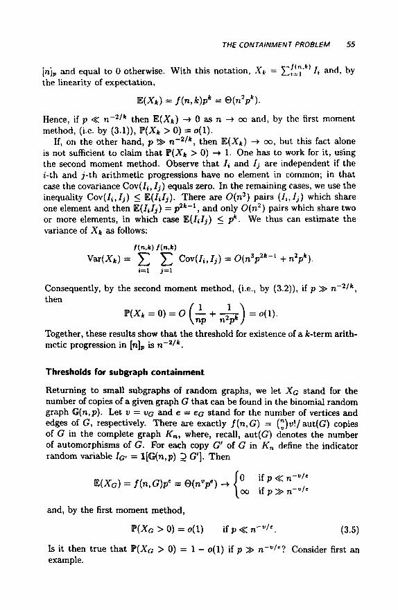
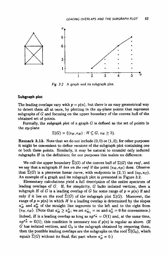
1 2 3 4 5 " Fig. 3.2 A graph and its subgraph plot.

Subgraph plot

The leading overlaps vary with p = p{n), but there is an easy geometrical way to detect them all at once, by plotting in the xy-plane points that represent subgraphs of G and focusing on the upper boundary of the convex hull of the obtained set of points.

Formally, the subgraph plot of a graph G is defined as the set of points in the iy-plane

Σ(0 = {(vH,eH) : H CG, v„ >2).

Remark 3.13. Note that we do not include (0,0) or (1,0); for other purposes it might be convenient to define versions of the subgraph plot containing one or both these points. Similarly, it may be natural to consider only induced subgraphs H in the definition; for our purposes this makes no difference.

We call the upper boundary E(G) of the convex hull of T,{G) the roof, and we say that a subgraph H lies on the roof if the point (VH, en) does. Observe that ¿(G) is a piecewise linear curve, with endpoints in (2,1) and (υσ,ββ). An example of a graph and its subgraph plot is presented in Figure 3.2.

Elementary calculations yield a full description of the entire spectrum of leading overlaps of G. If, for simplicity, G lacks isolated vertices, then a subgraph H of G is a leading overlap of G for some range of p = p(n) if and only if it lies on the roof £(G) of the subgraph plot E(G). Moreover, the range of p = p(n) in which if is a leading overlap is determined by the slopes ajj and a# of the straight line segments to the left and to the right from {VHICH)- (Note that a^ > α^; we set α^ = oo and a j = 0 for convenience.) Indeed, H is a leading overlap as long as npa» = 0(1) and, at the same time, npa» = Ω(1); this condition is necessary too if p(n) is regular as above. (If G has isolated vertices, and Go is the subgraph obtained by removing them, then the possible leading overlaps are the subgraphs on the roof S(Go), which equals S(G) without its final, flat part where aj¡ = O.)

64 SMALL SUBGRAPHS

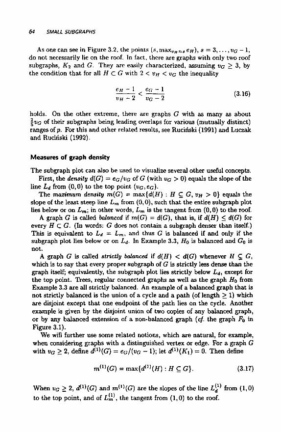
As one can see in Figure 3.2, the points (s, rnaxVH=s e//), s = 3 , . . . , VG - 1, do not necessarily lie on the roof. In fact, there are graphs with only two roof subgraphs, Ki and G. They are easily characterized, assuming VG > 3, by the condition that for all H C G with 2 < VH < VG the inequality

tJL^\ < e ~ (3.16) VH - 2 vG - 2 v '

holds. On the other extreme, there are graphs G with as many as about \VG of their subgraphs being leading overlaps for various (mutually distinct) ranges of p. For this and other related results, see Rucinski (1991) and Luczak and Rucinski (1992).

Measures of graph density

The subgraph plot can also be used to visualize several other useful concepts. First, the density d(G) = CG/VG oiG (with VG > 0) equals the slope of the

line Ld from (0,0) to the top point (να,εβ)· The maximum density m(G) = max{d(H) : H C G, VH > 0} equals the

slope of the least steep line Lm from (0,0), such that the entire subgraph plot lies below or on Lm; in other words, Lm is the tangent from (0,0) to the roof.

A graph G is called balanced if m(G) = d{G), that is, if d(H) < d{G) for every H C G. (In words: G does not contain a subgraph denser than itself.) This is equivalent to Ld = Lm, and thus G is balanced if and only if the subgraph plot lies below or on Ld- In Example 3.3, Ho is balanced and Go is not.

A graph G is called strictly balanced if d(H) < d(G) whenever H Q G, which is to say that every proper subgraph of G is strictly less dense than the graph itself; equivalently, the subgraph plot lies strictly below L¿t except for the top point. Trees, regular connected graphs as well as the graph H0 from Example 3.3 are all strictly balanced. An example of a balanced graph that is not strictly balanced is the union of a cycle and a path (of length > 1) which are disjoint except that one endpoint of the path lies on the cycle. Another example is given by the disjoint union of two copies of any balanced graph, or by any balanced extension of a non-balanced graph (c/. the graph FQ in Figure 3.1).

We will further use some related notions, which are natural, for example, when considering graphs with a distinguished vertex or edge. For a graph G with vG > 2, define SX\G) = eG/{vG ~ 1); let d<l>(A"i) = 0. Then define

m ( 1 )(G) = m a x { d ( 1 ) ( t f ) : f f C G } . (3.17)

When va > 2, él*>(G) and m ^ ^ G ) are the slopes of the line Ld1] from (1,0)

to the top point, and of Lm\ the tangent from (1,0) to the roof.

LEADING OVERLAPS AND THE SUBGRAPH PLOT 65

Similarly, for a graph G with vG > 3, define d(2)(G) - {ea - \)/{vG - 2); let d ( 2 ) (# i ) = d^(2Kl) = 0 and S2\K2) = 1/2. Then define

m[2){G) = max{d ( 2 )(#) :HCG). (3.18)

The definition of S2)(K2) may look artificial but turns out to be convenient (cf. Remark 3.14 below). Note that if eG > 2, then m (2 )(G) = max{d ( 2 )(#) : H CG, VH > 3}, so the special case does not matter.

When eG > 2, d(2){G) and mS2^{G) are the slopes of the line L(j] from (2,1) to the top point, and of Lm , the tangent from (2,1) to the roof.

In analogy with the above, a graph G is called Κχ-balanced if mSx^(G) = d (1)(G), or equivalent^, d^{H) < ^{G) for all H CG; furthermore, graphs with dll)(H) < d^{G) for all H C G are called strictly Ki-balanced. Anal-ogously, we define K2-balanced and strictly K2-balanced graphs. These no-tions have applications in the study of solitary subgraphs (see Section 3.6), G-factors (see Chapter 4), and Ramsey properties of random graphs (see Sec-tion 7.6 and Chapter 8).

R e m a r k 3.14. Below we collect some simple but useful facts about the pa-rameters m(G), mW(G) and m^(G). The proofs are left to the reader (Ex-ercise!).

For convenience, let m^(G) = m(G). Let G i , . . . , G * be the connected components of G. Then m^(G) = maxj m ^ G j ) for i = 0,1,2. This implies that strictly balanced, strictly Ki-balanced, and strictly /(^-balanced graphs are all connected.

We have m^(G) = 0 if and only if G is empty, that is, eG = 0, for every i. Moreover, m(G) < 1 if and only if G is a forest (and then m(G) = 1 - 1/e, where s is the order of the largest component), and m(G) = 1 if and only if the densest component of G is unicyclic. For all other graphs, m(G) > 1.

As far as m ( 1 )(G) is concerned, m^(G) = 1 if G is a non-empty forest, and m ^ ^ G ) > 1 if G is not a forest.

Finally, m(2)(G) = 1/2 when the maximum degree A(G) = 1 (i.e., when G consists of isolated edges and possibly some isolated vertices), m^2)(G) = 1 if G is a forest with A(G) > 2, and m^(G) > 1 if G is not a forest.

In Chapter 6, we will use the following observation.

Lemma 3.15. Ifnpm^ -» oo, then every leading overlap is connected.

Proof. Suppose that H CG with e« > 0. If H is the disjoint union of two proper subgraphs H\ and H2, where, say, e(Hi) > 0, then Lemma 3.6 yields nv(H2)pe(H2) _> OQ a n d t h u s

nv»pe" = η«(">)ρ'(">)ηυ(^)ρβ<^) > η ·(»ι)ρ«("ι> ~ E{XH,) > Φσ·

Consequently, H is not a leading overlap. ■

66 SMALL SUBGRAPHS

R e m a r k 3.16. For eG > 2, the slope a£ 3 defined above equals m(2)(G). Hence, under this condition, Ki is a leading overlap when npm ( G ) = Ω(1), and the only leading overlap when npm ^G^ -» oo.

R e m a r k 3.17. Assume VQ > 3. Then the condition (3.16) characterizing graphs G with only two roof subgraphs (viz. K2 and G) may be expressed as d ( 2 ) (# ) < d(2)(G) for all H ς G with vH > 3; this is equivalent (Exercise!) to G being strictly ^ -ba lanced , except for the two cases G = 2K2 and G being a union of an edge and an isolated vertex. Consequently, if G lacks isolated vertices, then G has only two possible leading overlaps if and only if G is strictly ^-ba lanced or G = 2Ki.

R e m a r k 3.18. The arboricity of a graph is defined as the least number of forests that together cover the edge set of the graph. This seemingly unrelated notion is, in fact, closely connected to the quantities just defined; by a theorem of Nash-Williams (1964) (see e.g. Diestel (1996)), the arboricity of G equals rm<»>(G)l.

3.3 SUBGRAPH COUNT AT THE THRESHOLD

When p = 0 ( n _ 1 / m ( G ) ) , we have Φ σ = θ(1) and, by Theorem 3.9,

0 < liminf P(G(n,p) D G) < limsupP(G(n,p) D G) < 1. n-Hx> n-K»

This ensures that the threshold in Theorem 3.4 cannot be sharpened. For this range of p = p(n) the derivation of limn_Kx, P(G(n,p) D G) may not be easy. However, for the class of strictly balanced graphs defined in the preceding section, not only the precise value of limn_»oo P(G(n>p) 3 G), but the entire limiting distribution of XG can be computed.

The following result was proved independently in Bollobas (1981b) and Karonski and Rucinski (1983a), and generalizes earlier results about trees (Erdös and Rényi 1960) and complete graphs (Schürger 1979).

Theorem 3.19. If G is a strictly balanced graph and np™^ -* c > 0, then XG -► Ρο(λ), the Poisson distribution with expectation λ = c" c /au t (G) .

Proof. This proof exemplifies the technique called the method of moments, which is presented in detail in Chapter 6; we use here the version given in Corollary 6.8.

Consider the factorial moments of XG, defined as E(Xc)k = E[XQ{XG -1) · · ■ {XG - k + 1)]. We have, for * = 1,2,. . . ,

E(XG)*= Σ Ρ(/σι···/σ. = 1) = ££ + ££', Gi Gk

SUBGRAPH COUNT AT THE THRESHOLD 67

where the summation extends over all ordered fc-tuples of distinct copies of G in Kn, and E'k is the partial sum where the copies in a fc-tuple are mutually vertex disjoint. It is easy to verify (Exercise!) that

E'k ~ (EXG)k ~ (c" c /aut(G))*.

This implies that XG is asymptotically Poisson if E'¿ = o(l), and it remains to be proved that E'k' = o(l). Let et be the minimum number of edges in a t-vertex union of k not mutually vertex disjoint copies of G.

Claim. For every k>2 and k <t < kvo, we have et > tm(G).

Proof of Claim. For a graph F define fp = m{G)vF - ep. Note that fa = 0 and, since G is strictly balanced, /// > 0 for every proper subgraph H of G. We are to prove that for every graph F which is a union of k not mutually vertex disjoint copies of G, ¡F < 0. We will do it by induction on A:, relying heavily on the modularity of / , that is, on the equality

/ F , U F 2 = / F , + ÍFt - ÍFxnFi (3.19)

valid for any two graphs F\ and F2 . Let F = U«=i £*»> where each G, is a copy of G, and the copies are numbered so that G\ Π G<i Φ 0. For k = 2, (3.19) yields / G , U C 2 = - / σ , η σ 2 < 0, because G\ Π G2 is a proper subgraph of G. For arbitrary k > 3 we let F' = [j^ G¿ and H = F' Π G*. Then H may be any subgraph of G including G itself and the null graph, but in any case fa > 0. Moreover, fp> < 0 by the induction assumption. Thus

fF = fF, + fGk -fH<0. ■

Having proven the claim, we easily complete the proof of Theorem 3.19 with one line. Indeed

kv-l

E'¿= £ 0 ( n y « ) = o(l). ■ t=k

R e m a r k 3.20. Using Theorem 6.10, Theorem 3.19 can be extended to joint convergence of several subgraph counts, with the limit variables independent (Exercise!).

Still assuming that p = 0 ( n - 1 / m ( G , ) ) , consider graphs other than strictly balanced graphs. If G is nonbalanced, then the expectation of XQ tends to infinity. It turns out that there is a nonrandom sequence a„(G) -»· 00, such that the asymptotic distribution of Xa/an{G) coincides with that of XH, where H is the largest subgraph of G for which d(H) = m{G). Clearly, H is balanced and we are back to the balanced case. The sequence an(G) is equal to the expected number of extensions of a given copy of H to a copy of G in the random graph G(n,p). For details, see Rucinski (1990).

68 SMALL SUBGRAPHS

If a graph G is balanced but not strictly balanced, then the limiting dis-tribution of XG is no longer Poisson. Although, in principle, as shown by Bollobas and Wierman (1989), the limiting distribution can be computed, there is no compact formula. We give only three simple examples, illustrating typical phenomena.

Example 3.21. We consider three balanced but not strictly balanced graphs. All three have m(G) = 1, and thus we assume p = c/n for some c > 0.

First, if G = 2C3, a union of two disjoint triangles, then a.a.s. XG = i X c 3 ( * c 3 - l ) (Exercise!). Since XCi Λ Z3 € Po(c3/6) by Theorem 3.19, and continuous functions preserve convergence of distribution (Billingsley 1968, Section 5), we obtain XG -* \Zz(Z$ — 1). In particular, for the probability of no copy of G, ?(XG = 0) -> (1 4- c 3 /6)exp(-c 3 /6) .

Second, if G is a disjoint union of a C3 and a C4, then a.a.s. XG = Xc3Xct ■ By Remark 3.20, (XC3,Xc<) -+ {Z3,Z4), with Z3 6 Po(c?/6) and ZA e Po(c4/8) independent. Consequently, XG -* Z3Z4. In particular, Ρ(ΛΌ = 0) -> 1 - (1 - exp(-c 3 /6) ) ( l - exp(-c 4 /8 ) ) .

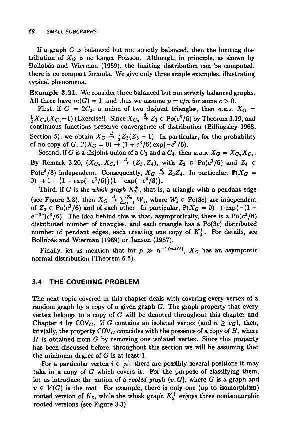
Third, if G is the whisk graph Kf, that is, a triangle with a pendant edge (see Figure 3.3), then XG -* Σ ^ ι W«> w n e r e W< € Po(3c) are independent of Z3 € P o ^ / ö ) and of each other. In particular, F(XG = 0) -> e x p ( - ( l -e _ 3 c )c 3 /6) . The idea behind this is that, asymptotically, there is a Po(c?/6) distributed number of triangles, and each triangle has a Po(3c) distributed number of pendant edges, each creating one copy of K$. For details, see Bollobás and Wierman (1989) or Janson (1987).

Finally, let us mention that for p » η~ι^"ι(·α\ XG has an asymptotic normal distribution (Theorem 6.5).

3.4 THE COVERING PROBLEM

The next topic covered in this chapter deals with covering every vertex of a random graph by a copy of a given graph G. The graph property that every vertex belongs to a copy of G will be denoted throughout this chapter and Chapter 4 by COVc- If G contains an isolated vertex (and n > VG), then, trivially, the property COVc coincides with the presence of a copy of H, where H is obtained from G by removing one isolated vertex. Since this property has been discussed before, throughout this section we will be assuming that the minimum degree of G is at least 1.

For a particular vertex i € [n], there are possibly several positions it may take in a copy of G which covers it. For the purpose of classifying them, let us introduce the notion of a rooted graph {v,G), where G is a graph and v € V(G) is the root. For example, there is only one (up to isomorphism) rooted version of A3, while the whisk graph K% enjoys three nonisomorphic rooted versions (see Figure 3.3).

WE COVERING PROBLEM 69

© * l

Fig. 3.3 Three rooted versions of the whisk graph; the roots are indicated by open circles.

For a rooted graph (i>,G), with vG > 1, let d(v,G) = eG/(vG - 1) and let

m(v,G)= maxι d(v,H).

(Thus, d{v,G) = d(1)(G) does not depend on v, but m(v,G) does, in general.) A rooted graph {v,G) is called balanced if d(v,G) = m(v,G) and strictly

balanced if d(v, H) < d(v, G) for every proper subgraph H of G containing the vertex v. For instance, among the three rooted versions of Kf only one is strictly balanced, while the other two are not balanced (Exercise!). Note that a graph is strictly K\ -balanced if and only if all its rooted versions are strictly balanced (Exercise!). In particular, all cycles and complete graphs have only one rooted version, and that is strictly balanced.

For i € [n] and v G V(G), let Ui{v) be the number of copies of (v,G) contained in the random graph G(n,p), in which vertex i takes the role of the root v, and let (/< be the total number of copies of G containing i. Then, similarly to the problem of containment of ordinary subgraphs, p = n~l^m^v,a^ is the threshold for the property uUi(v) > 0" (Rucinski and Vince 1986) and consequently, p = η- ι /"»η„€ο ">(».C) ¡ s the threshold for the property uUi > 0" (Exercise!).

For instance, as soon a s p » τι -3 ' '4 , a fixed vertex, say vertex 1, a.a.s. belongs to a copy of Kf, but only when p » n~2/3, does it belong to a triangle.

However, we are mainly interested in the random variable

i

which counts the vertices of G(n,p) not covered by copies of G; hence COVG is equivalent to "WQ = 0". Theorem 3.22 below provides thresholds for the events COVo which, of course, depend on the structure of G.

For a graph G, let m . = min„6c m(v, G) and M(G) = {v 6 V(G) : m(v, G) = m . } . For a vertex υ € M (G) let Cv be the family of all subgraphs H of G which contain v and satisfy the conditions d(v, H) = m . and NH(V) Φ 0,

70 SMALL SUBGRAPHS

the latter condition just saying that v is not an isolated vertex in H. Further, let sv = min//ecv e(H), with sv = oo if C„ = 0, and s = max r € M ( C ) s„. Finally, set a = |M(G) | /aut(G).

T h e o r e m 3.22. Let G be a graph with minimum degree at least 1.

(i) If for every v € M(G) the rooted graph (v,G) is stnctly balanced, then

hm P(G(n,p) 6 COVG) = I / 6

n-*°° yl if anv°-lpeG - logn -> oo.

Moreover, if anv°~lpea - logn -» c, -oo < c < oo, i/»en WG 4 Po(e _ c ) , and hence P(G(n,p) e COVc) -> e x p ( - e _ c ) .

(ii) If s < oo, then there exist constants c, C > 0 suc/ι i/iot

lim P(G(».p) € COVG) = i ° ^ < c ( l o g n ) ^ / - ,

(iii) If s = oo, ίΛβη

lim P(G(»,p) 6 COVG) = ( ° V / * " " ' / " ·

It is easy to check that the assumption in (i) is a special case of that in (ii), with m» = d^(G) and s = eG (Exercise!). In Case (iii), which is the complement of (ii), the parameter m . coincides with m{G) appearing in Theorem 3.4 (Exercise!); hence the threshold for covering by copies of G coincides with the threshold for existence of any copy at all.

R e m a r k 3.23. Note that the nicer the structure of G, the sharper thresh-old one can prove. Indeed, in Case (i), a~l/e° ( l o g n ) 1 / e c n - l / m · is a sharp threshold. In Case (ii), it follows from Theorem 1.31 that there exists a sharp threshold, although we do not know it exactly. By (ii) above, the sharp thresh-old is of the form &(n)(logn)1 ' '5n_1/m · for some b(n) with c < 6(n) < C; it is reasonable to conjecture that b(n) is a constant, but at present we cannot rule out the possibility that it oscillates somehow.

In Case (iii), in contrast, the threshold is coarse. In fact, if p = cn~llm" for any fixed c > 0, and H is a minimal subgraph of G such that d{H) = m{G),

d then Theorem 3.19 shows that XH -> Ρο(λ) for some λ < oo, and thus V{XG = 0) > ¥{XH =0)-¥ e~x > 0, so P(G(n,p) € C0VG) ■/> 1.

Part (i) was proved independently by Rucinski (1992a) and, in a slightly disguised form, by Spencer (1990). We will present the proof of part (i) only. The proofs of the other two parts follow from more general results by Spencer

THE COVERING PROBLEM 71

# # #

L\ Li L$

Fig. 3.4 The lollipop graphs.

(1990) on extension statements; see the end of this section. Before presenting the proof of (i), we give a few examples.

Example 3.24. The graphs K3 and K% have strictly balanced rooted ver-sions and, by Case (i) of Theorem 3.22, the respective thresholds for the properties COVK3 and COVK+ are (logn)1 /3?! - 2 /3 and ( l ogn ) 1 / 4 ^ - 3 ^ , re-spectively. In particular, for ( logn)1 / '4n - 3 /4 «C p(n) <C n - 2 / 3 a.a.s. every vertex belongs to a copy of Kf, but since there are only o(n) triangles, most vertices take the "off-triangle" position.

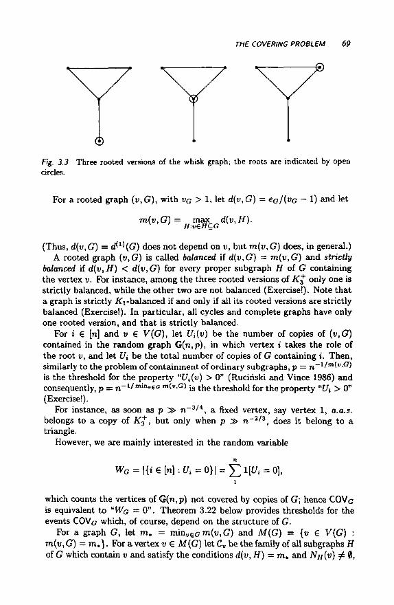
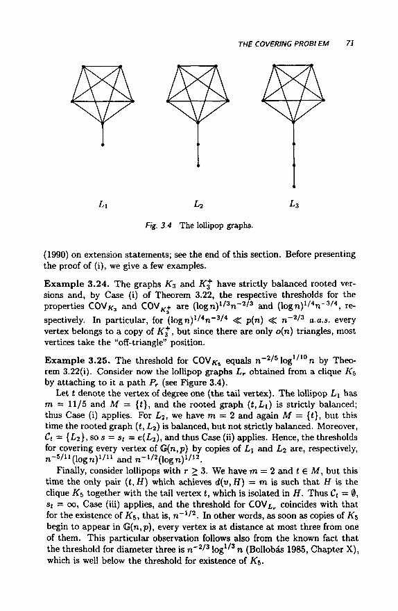
Example 3.25. The threshold for COV*, equals n _ 2 / 5 l o g 1 / I 0 n by Theo-rem 3.22(i). Consider now the lollipop graphs Lr obtained from a clique K5 by attaching to it a path Pr (see Figure 3.4).

Let t denote the vertex of degree one (the tail vertex). The lollipop Lx has m = 11/5 and M = {t}, and the rooted graph (t,Li) is strictly balanced; thus Case (i) applies. For Lj . w e have m = 2 and again M = {t}, but this time the rooted graph (t, L2) is balanced, but not strictly balanced. Moreover, Ct = {L2}, so s = st = e(L2), and thus Case (ii) applies. Hence, the thresholds for covering every vertex of G(n,p) by copies of L\ and L2 are, respectively, n - s / ^ l o g n ) 1 / 1 1 and n - ^ l o g n ) 1 / 1 2 .

Finally, consider lollipops with r > 3. We have m = 2 and t € M, but this time the only pair {t,H) which achieves d(v,H) — m is such that H is the clique ΛΓ5 together with the tail vertex t, which is isolated in H. Thus Ct = 0, st = 00, Case (iii) applies, and the threshold for COV¿r coincides with that for the existence of Ä5, that is, n - 1 / 2 . In other words, as soon as copies of K5 begin to appear in G(n,p), every vertex is at distance at most three from one of them. This particular observation follows also from the known fact that the threshold for diameter three is n

-2/3 l o g i /3 n (BoiioW« 1985, Chapter X), which is well below the threshold for existence of K$.

72 SMALL SUBGRAPHS

Proof of Theorem 3.22{\). We use a mixture of the second moment method and the correlation inequality of Theorem 2.18(i). By the monotonicity of the property COVQ we may assume that nv°~1pea = 0(logn). Since for every i; $ M(G), F(Ui(v) > 0) = o(l), the decisive role in covering the vertices of G(n,p) is played by the rooted versions (v,G), where v G M(G). Let {VJ}, i = 1 , . . . , / , be a maximal collection of vertices of M(G) for which the rooted graphs (VJ,G) are pairwise nonisomorphic. Set Üi = 5Z<=i U*(vi) anc* observe that

n ^ ^ = | Μ | Χ 0 . i= l

Hence, by symmetry, E(t/i) = ^ E{XG) = anv°-lpec + o(l). Further, for each v $ M(G), choose a minimal subgraph Hv C G containing

v such that d(v, Hv) = m(v,G) > m . , let U*(v) be the number of copies of (υ,Ηυ) in G(n,p) rooted at i, and let U¡ = ¿v*Af(G) U¡{v). Then Et/,* = o(l).

Since E(WC) = n F(U\ = 0), we need a sensitive asymptotic for P(f/i = 0). Note that Üx + U[ = 0 implies C/j = 0. Thus, by Corollary 2.13 we have

P(f/, = 0) > Ψψι + U{ = 0) > e - E ( & 1 + l / n / ( i -p ) = e-E(t7,)+c(i)

For an upper bound, let S be the family of all edge sets of rooted copies of {VJ,G), j = 1 , . . . , / , in the complete graph Kn with vertex 1 as the root. For each A £ S, we set

IA = l[ACG(n,p)}.

We then have

Σ Σ E(Wß) = o(En2"°"'"1p2ec-t

A Β^Α,ΒΓιΑφϊ \(»,t)

= 0 | η 2 ν 0 - 2 ρ 2 β 0 ^ η - ( . - 1 ) ρ - Λ

\ (».*) /

where s and t represent, respectively, the number of common vertices and edges of a pair of two copies of G, each rooted at a vertex of M{G) and both containing vertex 1 as the root. Such an intersection is a proper subgraph of G containing a vertex v e M(G) and hence, by the fact that (v,G) is strictly balanced, we always have

t eG s — 1 VQ — 1

Thus, in our range of p(n), n'~1pi > ne for some ε > 0. This together with Theorem 2.18(i) implies that

P(£/i = 0) < ?{0i = 0) < e - ^ 0 · ) ^ ' 1 ) .

THE COVERING PROBLEM 73

Hence,

E{WG) = ηΨ{υ1 = 0) = ne-E{0i)+o{l) = n e-«n V i '"Vc+·«1). (3.20)

If an°c~lpea - logn -► oo, then E(WG) = o(l) and, by the first moment method, ?(WG > 0) = o(l). On the other hand, if anVa~lpe° - logn -► -co, then E(WG) -> oo and we apply the second moment method to WG- TO this end, as WG is a sum of mutually dependent indicators, it is convenient to express the variance of WG in the form

Var(WG) = E(WG(WG - 1)) + E(WG) - (E(WG))2.

We have

E{WG{WG - 1)) = n{n - 1) Ψ(ϋι = U2 = 0) < n(n - 1) P(C/i = C72 = 0)

and, by another application of Theorem 2.18(i) (this time to the family of all edge sets of copies of (VJ,G), j = 1, . . . , / , rooted at 1 or 2),

P(ft = í / 2 = 0 ) < e - 2 E ( í ) ' ) + o ( 1 ) .

Altogether,

nw°-0)^¡ma)?- WWGW + mo)-l^°-Similarly one can prove that when anVG~lpea — logn -¥ c, and thus

E{WG) -> e~c by (3.20), the fc-th factorial moment E[WG(WG - 1) · ·· {WG -k + 1)] of WG converges to e~ck for every k > 1. This proves, by Corol-lary 6.8, that WG converges to the Poisson distribution with expectation e~c. Alternatively, one could apply here Stein's method (c/. Theorem 6.24). ■

Extension statements

Spencer (1990) considers a related problem with some applications to the zero-one laws for random graphs discussed in Chapter 10.

Let R = {vi,... ,vr} be an independent set of vertices in a graph G. The pair (R,G) will be dubbed a rooted graph. For |ñ | = 1 this is the notion introduced at the beginning of this section. We say that a graph F satisfies the extension statement Ext(i?,G), or briefly, F € Ext(ii,G), if for every r-tuple R' = {v[,...,v'r} of vertices of F there is a copy of G in F with v'j mapped onto u,, j = 1, . . . , r.

Example 3.26. If G = K2 and |ñ| = 1, then F 6 Ext(Ä, G) means that there are no isolated vertices in F. If G = K3 and \R\ = 1, then F 6 Ext(iZ,G) is equivalent to F € COVG- The same is true for every vertex-transitive graph G; more generally, if R = {v}, then F € Ext(iZ.G) means that every

74 SMALL SUBGRAPHS

vertex in F belongs to a copy of G where it corresponds to v. If G = P\, and ñ is the set of the endpoints of P*, then F € Ext(/Z, G) says that every pair of vertices of F is connected by a path of length k.

We will now define notions which are straightforward generalizations of the case (v,G) treated above. For a rooted graph (R, G), with r — \R\, let d(R,G) = eG/(va - r) and let

m(R,G) = max d(R,H). H RCHCG

The rooted graph (R, G) is called balanced if for every subgraph H of G, such that V{H) D R, we have d(R,H) < d(R,G), and strictly balanced if this inequality is strict for all proper subgraphs H of G, such that V(H) D R.

As a generalization of the families Cv appearing before Theorem 3.22 we now define a subgraph H containing R to be primal if d(R, H) = m{R, G) and grounded if at least one of vi,..., vT is not isolated in H. We let SR be the smallest number of edges in a grounded primal subgraph H, with SR = oo if no such subgraph exists. Finally, let 61 be the number of automorphisms of G that fix every element of fl, and let 02 be the number of permutations of R that can be extended to some automorphism of G. Then, the following results hold; for the proof we refer to Spencer (1990).

T h e o r e m 3.27. Let G be a graph with minimum degree at least I, and let R ψ$ be an independent set of vertices in G.

(i) / / the rooted graph (R, G) is strictly balanced, then

lim P(G(n,p) 6 Ext(fcG)) = { ° *"""?? ~ ^ ^ " -¥ - 0 0

- > OO.

Moreover, ifnvo~rp'G - birlogn -* c, - 00 < c < 00, then P(G(n,p) G Ext(Ä,G)) -*·βχρ(-ε-0 /6 ' /&2)

(ii) If SR < 00, inen iAere exist constants c, C > 0 sucA ίΛοί

(iii) If SR = 00, t'n w/itcn case m(R,G) — m(G), then

i U » P ( G ( » . p ) € E r t ( i i , G ) ) S = | 1 ^ > > n - 1 / m ( G ) .

DISJOINT COPIES 75

The 1-statements in parts (ii) and (iii) (with \R\ = 1) immediately imply the corresponding statements in Theorem 3.22. This is not so for the 0-statements, but the 0-statements in Theorem 3.22(ii, iii) follow by the same proofs as for the corresponding 0-statements in Theorem 3.27 given in Spencer (1990). (For the 0-statement in (iii), this is just applying Theorem 3.4.)

Example 3.28. For a graph G, one may ask what the threshold is for the property that for every vertex of G(n,p) the subgraph induced by its neigh-borhood contains a copy of G. Let G + K\ be the graph obtained by joining a new vertex w to every vertex of G. Then this property is equivalent to Ext({w},G + K\). For a strictly balanced (in the ordinary, unrooted sense) graph G, the rooted graph (w,G + K\) is strictly balanced and, by The-orem 3.27(i), the desired threshold is ( l o g n ) 1 / ( , ' c + e c ) n - " G / ( " c + e c ) (which coincides with the threshold for COVO+JC,) (Exercise!).

3.5 DISJOINT COPIES

In this section we consider a problem which will be further developed in Sec-tion 4.2. The question we address here is: How many disjoint copies of a given graph G are there in a random graph G(n,p)? As the disjointness may be meant with respect to vertices or with respect to edges, we define two ran-dom variables DG and DG equal to the cardinality of the largest collection of vertex- and edge-disjoint copies of G, respectively. Trivially, DG < DG < XG, but also DG < De

H for every non-empty subgraph H of G and DG < DVH for

every non-null subgraph H of G. Define

Φνα(η,ρ) = Φ£ Hf min{E(Xw) :HCG,v„>Q} = min(<I>G,n),

denote Φ^ = Φο, where Φο was defined in Section 3.1, and observe that Φ& -i- oo if and only if Φ^ -» oo (c/. Lemma 3.6). We know from Section 3.1 that when <t>G -> oo, then XH = © c ( E X w ) for H C G (since Φ'α -> oo implies Φ% -* oo) and thus DG = Oc($G) and De

G = 00{Φα). In fact, the above quantities provide the correct orders of magnitude for the two random variables in question.

Theo rem 3.29. If Φβ -> oo, then DG = QC($G) and DG = Qc{$eG).

Proof. The proof below is a slight modification of that from Kreuter (1996) and relies on the second moment method.

Consider first the vertex case and define an auxiliary graph Γ with vertices being the copies of G in G(n,p) and edges connecting pairs of copies with at least one vertex in common. Thus, vr = XG and ep = £ F XF, where the sum is taken over all unions F = Gi U Gi of two copies of G sharing at least one vertex. Also, any independent set of vertices in Γ corresponds to a vertex-disjoint collection of copies of G in G(n,p). Hence, it follows from the

76 SMALL SUBGRAPHS

Turan Theorem (see, e.g., Berge (1973, p. 282)) that

In view of this, all we need to show is that

"MW) (322) for every union F of two vertex-intersecting copies of G.

For convenience, set * F = nVFpeF and note that EX/? = θ(Φρ). The reason we prefer to use Ψ/r rather than EX// is the log-modularity property

holding for arbitrary graphs Fx and ί^. Note also that Φ// = 0(EX//) = Ω(Φ&) if H C G and uH > 0.

Now assume that F = Gi UG2, where Gi and G2 are two copies of G, and let H = Gi Π G2 have υ« > 0. Then

■x,.e(t,).e(Ä)-0(Ä). In order to bound XF by the same quantity as EXf we will apply Cheby-shev's inequality. For this we need to estimate the variance of XF, which, by Lemma 3.5, is of the order Φ/-./Φ/?. To bound, in turn, Φ'ρ from below, as-sume that L C Fwithe¿ >0andlet£< = LnGj.i = 1,2. Then L = LiUL2, LuH = (L!U/í)U(L2Ui/),and(LiUír)n(L2Ui/) = H. Two applications of the log-modularity of Φ yield

ΦLuH^LDH ^LiUH^L2VH^LnH Φ/ =

Φ Η Φ?/ Here Lx U H, L2 U H and L Π H are all subgraphs of G. Thus, if vLne > 0, t h e n * t = n ( ( ^ ) 3 / * 3 r ) ·

In the special case vmH = 0, the graphs L\ and L2 are disjoint and at least one of them is non-empty. Assume that e¿, > 0. Then, taking into account that Φ/,2 > Φ£ -> oo if vi7 > 0 and *¿ 2 = 1 otherwise, we obtain

Consequently,

Φ £ = Φ £ Ι Φ £ , > Φ Λ , = Ω ( ^ - ) ·

ΦΡ=πηηΕΧ/, = Ω ( ^ Λ et>o v φ» y and, using the log-modularity of Φ again,

*™-'(©-°G&)-'G&)

VARIATIONS ON THE THEME 77

Hence, by Chebyshev's inequality and the assumption that Φα -> oo,

P (xF > E XF + | | ) = 0{1/*VG) = o(l),

which proves (3.22) and completes the proof of Theorem 3.29 in the vertex case.

The proof for DG follows along the same lines. But instead of repeating the same argument for the edge case, we present an alternative approach involving Markov's and Talagrand's inequalities.

Building the auxiliary graph Γ in a similar way with the obvious modifi-cation that now the edges of Γ join edge-intersecting copies of G in G(n,p), we have, by Markov's inequality (1.3), that with probability at least | , ep < 4E(e r ) . We have 4E(e r ) < cx{EXG)2l^G, for some cx > 0, and thus, by (3.21) modified to the edge case, and by the fact that XG = 0 c ( E X o ) . there is another constant c2 > 0 such that DG > C2$G with probability at least, say, | .

Now, using Talagrand's inequality, we will convert \ to 1 - o ( l ) as required. As we are heading toward an application of Theorem 2.29, let us define Zi to be the indicator of the presence of the i-th edge of the random graph G(n,p), i = 1,2,. . . , N = ( j ) . Then DG - f(Zx ,...,ZN), where the function / clearly satisfies the Lipschitz condition (L) with all Cj = 1. The other assumption of Theorem 2.29, Condition (C), holds with the function φ{τ) = ear for integer r > 0 (and thus with φ(τ) = βσΓΓ1 * ° Γ a n v r e a l r > 0)· Indeed, for any integer r, and for any graph F containing r edge-disjoint copies of G, choose J to be the index set of all ear edges belonging to these copies. Then any other graph coinciding with F on the given edges contains r edge-disjoint copies of G too. Therefore, by (2.35) (c/. Example 2.33), for 0 < c3 < c2 and with t = (c2 - c3)$c,

F(D'a < α3Φα) < 2Y{DG < **'a)*(Dh > Γ<*Φ&1)

* 2 6 X P { - ( C 2 ίαζζ°)2 } = «Φ<-»(«&» = 4Β· ■ Note that the last bound in the proof provides yet another proof of the

right-hand inequality of Theorem 3.9. Indeed,

P(XG = o) = f(DeG = 0) < ?{D'0 < c3<bG).

3.6 VARIATIONS ON THE THEME

There are several other properties related to that of containing a copy of G. One such property is the containment of at least one induced copy of G in the random graph G(n,p). Another variation is counting only those copies of G which are vertex disjoint from all other copies of G contained in G(n,p).

78 SMALL SUBGRAPHS

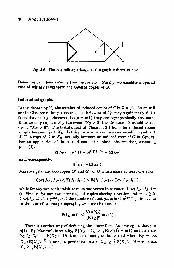
Fig. 3.5 The only solitary triangle in this graph is drawn in bold.

Below we call them solitary (see Figure 3.5). Finally, we consider a special case of solitary subgraphs: the isolated copies of G.

Induced subgraphs

Let us denote by YG the number of induced copies of G in G(n,p). As we will see in Chapter 6, for p constant, the behavior of YG may significantly differ from that of XG- However, for p = o(l) they are asymptotically the same. Here we only explain why the event "YG > 0" has the same threshold as the event "XG > 0". The 0-statement of Theorem 3.4 holds for induced copies simply because YG < XG- Let JG· be a zero-one random variable equal to 1 if G', a copy of G in K„, actually becomes an induced copy of G in G{n,p). For an application of the second moment method, observe that, assuming p = o(l),

E ( J G · ) = P e c ( l - p ) ( v ? ) - e o ~ E(JG<)

and, consequently, E{YG) ~ E{XG).

Moreover, for any two copies G' and G" of G which share at least one edge

Cov(JG>,JG") < E{JG'JG-) < WG-IG") ~ Cov(/G», JG..),

while for any two copies with at most one vertex in common, Cov( JQ· , Jc) = 0. Finally, for any two edge-disjoint copies sharing t vertices, where t > 2, COV(JG·, JG··) < P2e°, and the number of such pairs is 0{n2va~l). Hence, as in the case of ordinary subgraphs, we have (Exercise!)

There is another way of deducing the above fact. Assume again that p = o(l) . By Markov's inequality, ¥(XG -YG > \E(XG)) = o(l) and so a.a.s. YG > XG - J E ( A G ) · On the other hand, we know that when «$G -+ o°, XG/E(XG) A 1 and, in particular, a.a.s. XQ > | Ε ( Χ σ ) · Hence, a.a.s. V G > | E ( X G ) > 0 .

VARIATIONS ON THE THEME 79

The presence of an induced copy of G is not a monotone property (except in the trivial cases in which G is either complete or empty). It is not even convex (Exercise!), however, it has a second (disappearence) threshold toward the end of the evolution of G(n,p). In terms of q = 1 - p, it corresponds to the threshold for "XG° > 0" in the complementary random graph G(n,q), where Gc is the complement of G. Hence, the second threshold is roughly 1 - 0(n-1 /m<G '>) (Exercise!).

Solitary subgraphs

Let us denote by ZG the number of solitary copies of G. Clearly, ZQ < DG, where DG has been defined in the previous section. Observe that E(ZG) = E(XG)THG, where UQ is the conditional probability that a fixed copy of G is solitary, given that it is present in G(n,p).

For a nonbalanced G, limn_»oo P ( Z G > 0) = 0, since as soon as copies of G emerge, it can be seen by Theorem 2.18 that IIG is exponentially small with a power of n in the exponent, and hence P ( Z G > 0) < E ( Z G ) = Ε(ΛΌ)Πσ = o(l) (Exercise!). With some additional effort one can prove that for a balanced but not strictly balanced G, we have P( ZG > 0) = o(l) as soon as ¥(XG > 0) -► 1 and thus limsupP(ZG > 0) is never equal to 1 (Exercise!).

Let us assume now that G is strictly balanced. If p = Q(n~l^d^), then, as we showed in the proof of Theorem 3.19, a.a.s. there are no intersecting pairs of G at all, and so ZG = XG- In other words, when copies of a strictly balanced graph G first emerge, they are all solitary. This holds true even beyond the threshold, when npd^ -> oo sufficiently slowly. But the containment of a solitary copy is not monotone either, and with more and more edges in the random graph, the solitary copies of G become rarer until complete extinction occurs. The second (disappearence) threshold was detected for strictly K\-balanced graphs by Suen (1990), and for a slightly larger subclass of strictly balanced graphs (including trees) by Kurkowiak and Rucinski (2000). It is determined, roughly, by the equation EXQ = ©(nlogn).

The difficulty we are facing here is that the probablity Πσ depends on all pairs in [n]2 and, rather than finding an exact expression, one can only bound it, using results like Theorem 2.18 and Theorem 2.12. We remark that this problem was a motivation for Suen to develop his correlation inequality, some versions of which were discussed in Section 2.3.

Isolated subgraphs

A much simpler situation takes place when one counts the isolated copies of G, that is, assuming G is connected, the connected components of G{n,p) which are isomorphic to G. Let To count the isolated copies of G. This time E(TG) = E(yG)(l -pyo(n-vc) _ 0(n»Cp<ce-vCnp); h e n a ! ) ¡ f eQ > ^ w e

have P ( T G > 0) < E ( T G ) = o(l), and there are a.a.s. no isolated copies of G.

80 SMALL SUBGRAPHS

The same is true if &G = «c and further p <C 1/n or p » 1/n. We urge the reader (Exercise!) to show that TQ has a limiting Poisson distribution when G is connected with CQ = VG and p ~ c/n, 0 < c < oo (Erdös and Rényi I960); see Example 6.29.

It remains to consider connected graphs G such that ec < VG, that is, trees. These are the only small graphs which a.a.s. become components of a random graph. Instead of focusing on a single tree, we will count all trees of a given order at once. Let T„ denote the number of all v-vertex isolated trees in G(n,p), v = 1,2, — Then, provided np2 -*■ 0,

Ε(Γ„) = fnV"~V"1(l -ρΓ,η-")+(;)-υ+1 ~ ! ^ n V \V/ VI

υ - l g - w n p

This quantity converges to a constant if either rfp"'1 -> c > 0 or vnp — logn - (v - 1) log log n -> c G (-00,00). The following result, proved al-ready by Erdös and Rényi (1960), asserts that these two conditions determine two thresholds for the property Tv > 0. (See also Theorem 6.38 and Exam-ple 6.29.)

T h e o r e m 3.30. Let c„ = vnp - logn - {v - 1) log logn. Then

or c„ -» 00, Í0 i / n y - ' - ) 0 \l i / n V " 1 -> oc W > 0 ) ,, ._._.., . ^ ^ , ^ . ^

Moreover, if ηνρυ~ι - t e e (-00,00) or c„ -+ c > 0, ί/ien Tv -> Po(A), where λ = limn-»«, E(T„) € (0,00). ■

The case v = 1 is special here. The random variable ΤΊ is the number of isolated vertices in G(n,p) and nvpv~x — n. Hence there is only one threshold. Furthermore, the log logn term drops out and we arrive at the following corollary.

Corol lary 3 .31 . Let cn = np - logn and let T\ be the number of isolated vertices in G(n,p). Then

P(Ti > 0) (0 ifcn-+ 00, 1 ¿/ cn -► -00 .

Moreover, if cn -> c € (-00,00), then Ti -> Po(e c ) . ■

The proof of Theorem 3.30 follows the lines of those of Theorems 3.4, 3.19 and 3.22 (Exercise!). Another proof will be given in Example 6.28.